energy design analysis and evaluation of a proposed air rescue and
TRANSCRIPT

Energy Design Analysis and Evaluation of a Proposed Air Rescue and Fire Fighting Administration Building for Teterboro Airport
July 2003 • NREL/TP-550-33294
B. Griffith, S. Pless, B. Talbert, M. Deru, and P. Torcellini
National Renewable Energy Laboratory 1617 Cole Boulevard Golden, Colorado 80401-3393 NREL is a U.S. Department of Energy Laboratory Operated by Midwest Research Institute • Battelle • Bechtel
Contract No. DE-AC36-99-GO10337

National Renewable Energy Laboratory 1617 Cole Boulevard Golden, Colorado 80401-3393 NREL is a U.S. Department of Energy Laboratory Operated by Midwest Research Institute • Battelle • Bechtel
Contract No. DE-AC36-99-GO10337
July 2003 • NREL/TP-550-33294
Energy Design Analysis and Evaluation of a Proposed Air Rescue and Fire Fighting Administration Building for Teterboro Airport
B. Griffith, S. Pless, B. Talbert, M. Deru, and P. Torcellini Prepared under Task No. BEC2.4005

NOTICE This report was prepared as an account of work sponsored by an agency of the United States government. Neither the United States government nor any agency thereof, nor any of their employees, makes any warranty, express or implied, or assumes any legal liability or responsibility for the accuracy, completeness, or usefulness of any information, apparatus, product, or process disclosed, or represents that its use would not infringe privately owned rights. Reference herein to any specific commercial product, process, or service by trade name, trademark, manufacturer, or otherwise does not necessarily constitute or imply its endorsement, recommendation, or favoring by the United States government or any agency thereof. The views and opinions of authors expressed herein do not necessarily state or reflect those of the United States government or any agency thereof.
Available electronically at http://www.osti.gov/bridge
Available for a processing fee to U.S. Department of Energy and its contractors, in paper, from:
U.S. Department of Energy Office of Scientific and Technical Information P.O. Box 62 Oak Ridge, TN 37831-0062 phone: 865.576.8401 fax: 865.576.5728 email: [email protected]
Available for sale to the public, in paper, from:
U.S. Department of Commerce National Technical Information Service 5285 Port Royal Road Springfield, VA 22161 phone: 800.553.6847 fax: 703.605.6900 email: [email protected] online ordering: http://www.ntis.gov/ordering.htm
Printed on paper containing at least 50% wastepaper, including 20% postconsumer waste

iii
Contents
List of Tables ...................................................................................................................................v
List of Figures ................................................................................................................... ………vii
Acronyms..................................................................................................................................... viii
Acknowledgments.......................................................................................................................... ix
Executive Summary.........................................................................................................................1
1.0 Introduction................................................................................................................................3 1.1 Design Process .....................................................................................................................3 1.2 Project Summary..................................................................................................................4 1.3 Organization of Report ........................................................................................................4
2.0 Predesign Energy Simulations and Review of Office Areas .....................................................6 2.1 Base-Case Analysis..............................................................................................................6 2.2 Predesign Parametric Elimination........................................................................................7 2.3 Energy Efficient Predesigns...............................................................................................11
2.3.1 Energy Efficient Predesign #1 ..................................................................................11 2.3.2 Energy Efficient Predesign #2 ..................................................................................12 2.3.3 Energy Efficient Predesign #3 ..................................................................................12 2.3.4 Energy Efficient Predesign #4 ..................................................................................12
2.4 Predesign Recommendations .............................................................................................14
3.0 Baseline Analysis.....................................................................................................................15 3.1 Baseline Building Performance Model ..............................................................................18 3.2 Baseline Energy Model......................................................................................................19 3.3 Baseline Energy Costs .......................................................................................................20 3.4 Baseline Thermal Comfort.................................................................................................21
4.0 Elimination Parametric Study..................................................................................................23
5.0 Improved Energy Designs........................................................................................................24 5.1 Envelope Constructions .....................................................................................................24 5.2 Daylighting with Skylights ................................................................................................26 5.3 Overhangs and Clerestories ...............................................................................................28 5.4 Demand-Controlled Ventilation.........................................................................................33 5.5 HVAC Systems..................................................................................................................35
5.5.1 Office Zone DX Equipment......................................................................................35 5.5.2 Garage Zone Heater/Ventilators ...............................................................................37
6.0 Renewable Electricity Production............................................................................................39 6.1 Photovoltaic Modeling in PVSyst......................................................................................39 6.2 Photovoltaic Modeling in EnergyPlus ...............................................................................42
7.0 Discussion of Modeling Results ..............................................................................................43 7.1 Envelope ............................................................................................................................43 7.2 Daylighting with Skylights ................................................................................................44

iv
7.3 Overhangs and Clerestories ...............................................................................................44 7.4 Ventilation..........................................................................................................................44 7.5 HVAC Systems..................................................................................................................44
7.5.1 Office Zones..............................................................................................................45 7.5.2 Garage Zones ............................................................................................................45
7.6 Photovoltaics......................................................................................................................46 7.7 Results Summary ...............................................................................................................46
8.0 Design Recommendations .......................................................................................................48 8.1 Floor Plan Issues ................................................................................................................48 8.2 Building Envelope Issues...................................................................................................48 8.3 Daylighting Issues..............................................................................................................48 8.4 HVAC System Design .......................................................................................................49
9.0 Conclusions and Future Research............................................................................................51 9.1 General Conclusions ..........................................................................................................51 9.2 Future Research .................................................................................................................51
References......................................................................................................................................53
Appendix A. Predesign Program Summary...................................................................................54
Appendix B. Outdoor Temperature Histogram ............................................................................58
Appendix C. EnergyPlus Input Files ............................................................................................59
Appendix D. Economic Modeling of EnergyPlus Results............................................................61
Appendix E. DX Coil Performance Curves ..................................................................................63
Appendix F. Comparison of DOE-2.1E and EnergyPlus .............................................................68

v
List of Tables Table 1-1. Nine-Step Design Process for Designing and Constructing Energy Efficient Buildings..........3 Table 1-2. Original Project Timeline..........................................................................................................4 Table 2-1. Office Predesign Base-Case Parameters ...................................................................................6 Table 2-2. Office Predesign Base-Case Annual Energy Use and Costs .....................................................7 Table 2-3. Parametric Study Results for Energy Use for Predesign Dayshift Offices ...............................8 Table 2-4. Parametric Study Results for Energy Cost for Predesign Dayshift Offices ..............................9 Table 2-5. Heat Recovery, Night Ventilation, Daylighting, and EE #1 Energy Cost Analysis for
Predesign Dayshift Offices......................................................................................................11 Table 2-6. Base-Case Energy Costs Compared with Energy Efficient Predesigns ..................................12 Table 3-1. Thermal Zone Description: Internal Gains..............................................................................16 Table 3-2. Thermal Zone Description: Geometry.....................................................................................16 Table 3-3. Envelope Specifications for Baseline Models per ASHRAE 90.1-2001.................................17 Table 3-4. Zone Air Temperature Set Points ............................................................................................18 Table 3-5. Baseline Building Performance Model Results for Energy Use .............................................19 Table 3-6. Baseline Building Performance Model Results for Peak Loads..............................................19 Table 3-7. Baseline Energy Model Results for Energy Use .....................................................................20 Table 3-8. Baseline Energy Model Results for Energy Costs...................................................................21 Table 3-9. Summary of Baseline Performance Model Predictions for Occupant Thermal Comfort on
ASHRAE Thermal Sensation Scale for Uncooled Garages and Shops...................................21 Table 3-10. Summary of Baseline Building Performance Model Predictions for Occupant Thermal
Comfort on ASHRAE Thermal Sensation Scale for Heating in 24-Hour Offices ..................22 Table 3-11. Summary of Baseline Energy Model Predictions for Occupant Thermal Comfort on
ASHRAE Thermal Sensation Scale for 24-Hour Office and Garage......................................22 Table 4-1. Summary of Baseline Parametric Study by Type of Zone ......................................................23 Table 5-1. Envelope Thermal Performance Levels ..................................................................................25 Table 5-2. Summary of Results for Energy Use and Peak Loads: Envelope Change Models .................25 Table 5-3. Summary of Occupant Thermal Comfort Predictions on ASHRAE Thermal Sensation Scale
for Uncooled Garages and Shops: Envelope Change Models.................................................26 Table 5-4. Summary of Occupant Thermal Comfort Predictions on ASHRAE Thermal Sensation Scale
for Heating in 24-Hour Offices: Envelope Change Models ....................................................26 Table 5-5. Modeling of Lighting Controls for Daylighting......................................................................27 Table 5-6. Summary of Results for Energy Use and Peak Loads:............................................................27 Daylighting with Skylights Models ............................................................................................................27 Table 5-7. Summary of Occupant Thermal Comfort Predictions on ASHRAE Thermal Sensation Scale
for Uncooled Garages and Shops: Daylighting with Skylights Model ...................................28 Table 5-8. Summary of Occupant Thermal Comfort Predictions on ASHRAE Thermal Sensation Scale
for Heating in 24-Hour Offices: Daylighting with Skylights Model.......................................28 Table 5-9. Summary of Results for Energy Use and Peak Loads: Overhangs and Clerestories Model ...32 Table 5-10. Summary of Occupant Thermal Comfort Predictions on ASHRAE Thermal Sensation Scale
for Uncooled Garages and Shops: Overhangs and Clerestories Model...................................32 Table 5-11. Summary of Occupant Thermal Comfort Predictions on ASHRAE Thermal Sensation Scale
for Heating in 24-Hour Offices: Overhangs and Clerestories Model......................................33 Table 5-12. Summary of Results for Energy and Load in Demand-Controlled Garage/Shop/ARFF
Spaces......................................................................................................................................34

vi
Table 5-13. Summary of Predictions for Occupant Thermal Comfort on ASHRAE Thermal Sensation Scale for Uncooled Garages and Shops: Demand-Controlled Ventilation and Baseline Performance Model .................................................................................................................34
Table 5-14. Summary of Results for Energy Use for Office Zones with Constant-Volume DX Rooftop-Packaged Units ........................................................................................................................35
Table 5-15. Summary of Results for Energy Cost for Office Zones with Constant-Volume DX Rooftop-Packaged Units ........................................................................................................................36
Table 5-16. Summary of Predictions for Occupant Thermal Comfort on ASHRAE Thermal Sensation Scale for 24-Hour Office: ZN1................................................................................................36
Table 5-17. Summary of Results for Energy Use in Garage Zones............................................................37 Table 5-18. Summary of Energy Cost Results for Garage Zones...............................................................37 Table 5-19. Summary of Predictions for Occupant Thermal Comfort on ASHRAE Thermal Sensation
Scale for 24-Hour Garages: ZN3.............................................................................................38 Table 6-1. Summary of Predicted PV Performance by Month: 32° Tilt...................................................41 Table 7-1. Summary of Results for Energy Use for Entire Building........................................................47 Table 7-2. Summary of Results for Energy Cost for Entire Building.......................................................47 Table A-1. Administration/ARFF Building Program................................................................................54 Table C-1. Selected EnergyPlus Input Files Available from Modeling Effort..........................................59 Table D-1. Energy Prices...........................................................................................................................61 Table E-1. Example DX Coil Performance Data Table ............................................................................63 Table F-1. DOE-2.1E Whole Building Elimination Results Summary ....................................................69 Table F-2. EnergyPlus Whole Building Elimination Results Summary...................................................70
vii
List of Figures
Figure 2-1. Predesign base-case zone diagram ............................................................................................ 7 Figure 2-2. Parametric study results for energy use for predesign dayshift offices ..................................... 8 Figure 2-3. Parametric study results for energy cost for predesign dayshift offices.................................... 9 Figure 2-4. Lighting and HVAC energy cost comparison for base-case and energy efficient predesigns 13 Figure 2-5. Base-case lighting and HVAC energy costs by category ........................................................ 13 Figure 2-6. EE #4 lighting and HVAC costs with savings from base case................................................ 13 Figure 3-1. Thermal zones used in design development models ............................................................... 17 Figure 3-2. Weekday schedules for occupancy, lighting, and equipment.................................................. 18 Figure 5-1. Roof plan: skylight layout ....................................................................................................... 27 Figure 5-2. South-facing overhang design ratios, latitude 40.70 N ........................................................... 29 Figure 5-3. Clerestory and overhang layout............................................................................................... 30 Figure 5-4. Atrium modeling for daylighting............................................................................................. 31 Figure 6-1. 20-kWp PV system schematic................................................................................................. 39 Figure 6-2. Current-voltage curves of system losses and performance at expected envir. conditions....... 40 Figure 6-3. PV array tilt optimization ........................................................................................................ 41 Figure 6-4. Global horizontal insolation histogram by season................................................................... 42 Figure B-1. Typical year outdoor temperature histogram .......................................................................... 58 Figure E-1. Plot of example of biquadratic curve for capacity as a function of temperatures ................... 64 Figure E-2. Plot of example of biquadratic curve for energy input ratio as a function of temperatures .... 65 Figure E-3. Plot of an example quadratic performance curve for capacity as a function of flow rate ....... 66 Figure E-4. Plot of an example quadratic performance curve for energy input ratio as a function of flow
rate........................................................................................................................................... 66 Figure F-1. DOE-2 results for parametric elimination study of proposed Teterboro Airport Building .... 68 Figure F-2. EnergyPlus results for parametric elimination study of proposed Teterboro Airport
Building................................................................................................................................... 69

viii
Acronyms AC alternating current ACH air changes per hour ASHRAE American Society of Heating, Refrigerating, and Air-Conditioning Engineers CO2 carbon dioxide COP coefficient of performance CV constant volume air system DC direct current DHW domestic hot water DOE U.S. Department of Energy DX direct expansion, electric air-to-air cooling equipment EIR energy input ratio, inverse of COP GSHP ground source heat pump HPBi High-Performance Building research initiative (DOE) HRV heat recovery ventilator HVAC heating, ventilating, and air-conditioning IAQ indoor air quality IGU insulated glazing unit IP inch-pound (unit) NREL National Renewable Energy Laboratory PANYNJ Port Authority of New York and New Jersey PLF part load factor PLR part load ratio PMV predicted mean vote PV photovoltaics SHGC solar heat gain coefficient TMY typical meteorological year TMY2 typical meteorological year, updated format VAV variable air volume system

ix
Acknowledgments The authors would like to thank reviewers Tom Wood, Drury Crawley, and Sheila Hayter for their efforts and helpful comments. The U.S. Department of Energy’s High-Performance Buildings Research initiative (Office of Building Technologies) and the Photovoltaics (PV) for Buildings task (Office of Solar Energy Technology) supplied funding. The High Performance Buildings Research Initiative supported the energy design analysis reported here, and the PV for Buildings task supported the PV system analysis.

1
Executive Summary The High Performance Buildings Research group at the National Renewable Energy Laboratory conducts research for the U.S. Department of Energy’s High Performance Building initiative (HPBi), which focuses on greatly reducing energy use in commercial buildings. Actual buildings are used as case studies so that investigators can explore how “whole-building” and “system-integration” issues related to energy efficiency play out in the real world. A new/proposed building for the Teterboro Airport, just north of Newark, New Jersey, was selected as a case study for HPBi research efforts. This report documents research-level energy analysis conducted on the Teterboro Airport building during predesign and design phases of the project. The report’s goals are
• To provide specific analysis and recommendations intended to help the Teterboro Airport building achieve a goal of reducing energy cost by 50% or more compared to an equivalent code-compliant building
• To demonstrate analysis methodologies that are generally useful for designing extremely efficient commercial buildings
• To present examples of using EnergyPlus to conduct such analyses.
The design analysis involved the extensive use of computer simulations. An early simulation study, prepared during the predesign stage, was based on a two-story, solar-neutral building with a square floor plan and uniform glazing on all sides that could meet the program needs for office-type space. Using the program DOE-2.1E, we developed and modeled an energy efficient predesign. This analysis predicted a 44% reduction in energy cost over the base-case office building, which just met American Society of Heating, Refrigerating, and Air-Conditioning Engineers (ASHRAE) Energy Standard 90.1-1999. The project’s architects generated a proposed design, termed the Stage One design (dated December 14, 2001), which was subsequently analyzed using EnergyPlus to conduct extensive whole-building, annual energy simulations (Crawley 2001). The baseline model for this stage differed from the predesign base case in that it used the actual proposed building plan and enclosure designed to just meet ASHRAE 90.1-2001 (proposed informational Appendix [g]) requirements, rather than a square, 90.1-1999-compliant building). The design analysis showed that energy costs for conditioning, lighting, and ventilating offices could be reduced by 50.5% compared to a baseline building. For garage, shop, and maintenance spaces, energy costs for heating, lighting, and ventilating could be reduced by 48.3% compared to the baseline building. On an area basis, the overall energy use could be decreased from a baseline intensity of 245 kWh/m2·yr (77.7 kBtu/ft2·yr) to 79 kWh/m2·yr (25 kBtu/ft2·yr). Energy cost intensity could be reduced from $25.0/m2·yr ($2.32/ft2·yr) to $12.7/m2·yr ($1.18/ft2·yr). In this report, we show how these savings can be obtained by presenting results of energy models. In addition, we make specific design recommendations for the Teterboro Airport building, which include:
• Implementing aggressive daylighting design and lighting reductions. • Using high-performance glazing systems. • Adding skylights, clerestories, and overhangs. • Downsizing heating, ventilating, and air-conditioning (HVAC) equipment. • Adding heat recovery ventilation equipment. • Implementing demand-controlled ventilation. • Using variable air volume (VAV) air systems. • Selecting high-efficiency cooling equipment.

2
Occupant thermal comfort is also quantified, and the results show that energy savings can be obtained at the same time that occupant thermal comfort is improved. We present the following general conclusions in this report:
• The goal of reducing building energy costs by 50% compared to ASHRAE 90.1-2001(g) is attainable in a climate typical of the central East Coast of the United States for small to medium-sized commercial buildings with roughly half office and half light-industrial activities and partial 24-hour operation.
• Proposed informational Appendix (g) for ASHRAE Energy Standard 90.1-2001 is useful when calculating baseline energy use for determining energy savings.
• EnergyPlus has been developed to the point where it can be used to analyze building energy design for some, but not all, HVAC systems.
• The versatile capabilities of EnergyPlus for specifying schedules facilitate modeling demand-controlled ventilation schemes.
We recommend the following additional energy analysis for the Teterboro Airport building:
• As designs evolve for the Teterboro Airport building, energy models should be continually updated to ensure that the impact on energy efficiency is understood.
• As designs evolve for interior layout, furniture, and finishes, accurate daylighting models should be developed to predict natural lighting levels and to assist with properly locating daylight sensors.
• Many efforts to model VAV HVAC packaged systems in EnergyPlus were unsuccessful. Further efforts to model VAV packaged systems are warranted because of the potential to reduce high fan energy and costs.
• Centralized ground source heat pump modeling is warranted. • Nighttime ventilation precooling modeling is warranted. • Airflow models of the type known as “multizone” could be applied to assess the effectiveness of
passively ventilating the garage and shop spaces by leaving the garage doors open. This would save considerable fan power because the ventilation fans would be switched off.
• Heat recovery ventilation equipment needs to be modeled with lockout/bypassing because it is detrimental during free-cooling modes.

3
1.0 Introduction As part of the U.S. Department of Energy’s (DOE) High Performance Building initiative (HPBi), the High Performance Buildings Research group at the National Renewable Energy Laboratory (NREL) conducts research focused on greatly reducing the energy use in commercial buildings. Actual building projects are used as case studies so that investigators can explore how “whole-building” and “system integration” issues related to energy efficiency play out in the real world. A new/proposed building for the Teterboro Airport, located just north of Newark, New Jersey, was selected as a case study for research. For buildings that are not yet built, research focuses on changing the process by which buildings are designed. Part of this process change involves the extensive use of building energy simulation during the design phase, which offers designers energy-related data that can help them to understand the consequences of design decisions.
1.1 Design Process The group’s research focuses on the process by which an energy efficient commercial building can be designed, built, and operated. Encouraging the adoption of a process that has a better chance of producing energy efficient buildings is important because the conventional design process has not done an adequate job of integrating existing technologies. Hayter et al. (2000) describes an energy efficient design process in the nine steps listed in Table 1-1. In this report, we give examples of using energy simulation during predesign and design development phases, and document how steps 1 through 6 in Table 1-1 were applied to the new building for Teterboro Airport.
Table 1-1. Nine-Step Energy Design Process for Designing and Constructing Energy Efficient Buildings
STEP 1. CREATE A BASE-CASE BUILDING MODEL TO QUANTIFY BASE-CASE ENERGY USE AND COSTS. THE BASE-CASE BUILDING IS SOLAR NEUTRAL (EQUAL GLAZING AREAS ON ALL WALL ORIENTATIONS) AND MEETS THE REQUIREMENTS OF APPLICABLE ENERGY EFFICIENCY CODES SUCH AS ASHRAE* STANDARDS 90.1 AND 90.2. STEP 2. COMPLETE A PARAMETRIC ANALYSIS TO DETERMINE SENSITIVITIES TO SPECIFIC LOAD COMPONENTS. SEQUENTIALLY ELIMINATE LOADS, SUCH AS CONDUCTIVE LOSSES, LIGHTING LOADS, SOLAR GAINS, AND PLUG LOADS, FROM THE BASE-CASE BUILDING.
Predesign
STEP 3. DEVELOP PRELIMINARY DESIGN SOLUTIONS. THE DESIGN TEAM BRAINSTORMS POSSIBLE SOLUTIONS THAT MAY INCLUDE STRATEGIES TO REDUCE LIGHTING AND COOLING LOADS BY INCORPORATING DAYLIGHTING OR TO MEET HEATING LOADS WITH PASSIVE SOLAR HEATING. STEP 4. INCORPORATE PRELIMINARY DESIGN SOLUTIONS INTO A COMPUTER MODEL OF THE PROPOSED BUILDING DESIGN. ENERGY IMPACT AND COST EFFECTIVENESS OF EACH VARIANT IS DETERMINED BY COMPARING THE ENERGY WITH THE ORIGINAL BASE-CASE BUILDING AND TO THE OTHER VARIANTS. THOSE VARIANTS WITH THE MOST FAVORABLE RESULTS SHOULD BE INCORPORATED INTO THE BUILDING DESIGN.
Schematic Design
STEP 5. PREPARE PRELIMINARY SET OF CONSTRUCTION DRAWINGS.
Design Development
STEP 6. IDENTIFY AN HVAC† SYSTEM THAT WILL MEET THE PREDICTED LOADS. THE HVAC SYSTEM SHOULD WORK WITH THE BUILDING ENVELOPE AND EXPLOIT THE SPECIFIC CLIMATIC CHARACTERISTICS OF THE SITE FOR MAXIMUM EFFICIENCY. OFTEN, THE HVAC SYSTEM IS MUCH SMALLER THAN IN A TYPICAL BUILDING.
Construction Documents
and Bid
STEP 7. FINALIZE PLANS AND SPECIFICATIONS. ENSURE THAT THE BUILDING PLANS ARE PROPERLY DETAILED AND THAT THE SPECIFICATIONS ARE ACCURATE. THE FINAL DESIGN SIMULATION SHOULD INCORPORATE ALL COST-EFFECTIVE FEATURES.
4
Construction
STEP 8. RERUN SIMULATIONS BEFORE DESIGN CHANGES ARE MADE DURING CONSTRUCTION. VERIFY THAT CHANGES WILL NOT ADVERSELY AFFECT THE BUILDING’S ENERGY PERFORMANCE.
Occupancy
STEP 9. COMMISSION ALL EQUIPMENT AND CONTROLS (A BUILDING THAT IS NOT PROPERLY COMMISSIONED WILL NOT MEET THE ENERGY EFFICIENCY DESIGN GOALS). EDUCATE BUILDING OPERATORS (BUILDING OPERATORS MUST UNDERSTAND HOW TO PROPERLY OPERATE THE BUILDING TO MAXIMIZE ITS PERFORMANCE).
*ASHRAE: AMERICAN SOCIETY OF HEATING, REFRIGERATING, AND AIR-CONDITIONING ENGINEERS. †HVAC: HEATING, VENTILATING, AND AIR-CONDITIONING.
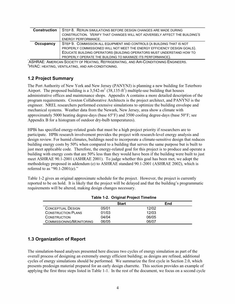
1.2 Project Summary The Port Authority of New York and New Jersey (PANYNJ) is planning a new building for Teterboro Airport. The proposed building is a 3,542-m2 (38,135-ft2) multiple-use building that houses administrative offices and maintenance shops. Appendix A contains a more detailed description of the program requirements. Croxton Collaborative Architects is the project architect, and PANYNJ is the engineer. NREL researchers performed extensive simulations to optimize the building envelope and mechanical systems. Weather data from the Newark, New Jersey, area show a climate with approximately 5000 heating degree-days (base 65°F) and 3500 cooling degree-days (base 50°F; see Appendix B for a histogram of outdoor dry-bulb temperatures). HPBi has specified energy-related goals that must be a high project priority if researchers are to participate. HPBi research involvement provides the project with research-level energy analysis and design review. For humid climates, buildings need to incorporate a climate-sensitive design that reduces building energy costs by 50% when compared to a building that serves the same purpose but is built to just meet applicable code. Therefore, the energy-related goal for this project is to produce and operate a building with energy costs that are 50% less than they would have been if the building were built to just meet ASHRAE 90.1-2001 (ASHRAE 2001). To judge whether this goal has been met, we adopt the methodology proposed in addendum (e) to ASHRAE standard 90.1-2001 (ASHRAE 2002), which is referred to as “90.1-2001(e).” Table 1-2 gives an original approximate schedule for the project. However, the project is currently reported to be on hold. It is likely that the project will be delayed and that the building’s programmatic requirements will be altered, making design changes necessary.
Table 1-2. Original Project Timeline Start End
CONCEPTUAL DESIGN 05/01 12/02 CONSTRUCTION PLANS 01/03 12/03 CONSTRUCTION 04/04 06/05 COMMISSIONING/MONITORING 06/05 06/07
1.3 Organization of Report The simulation-based analyses presented here discuss two cycles of energy simulation as part of the overall process of designing an extremely energy efficient building; as designs are refined, additional cycles of energy simulations should be performed. We summarize the first cycle in Section 2.0, which presents predesign material prepared for an early design charrette. This section provides an example of applying the first three steps listed in Table 1-1. In the rest of the document, we focus on a second cycle

5
of energy analysis to support design development, where modeling is able to use the specifics of a proposed layout rather than a generic, solar-neutral building. Although Section 2.0 presents predesign analysis, the bulk of this report presents design analysis of a “Stage One” design (dated December 14, 2001) represented by architectural drawings received from the PANYNJ called Plan Scheme “A” and Enclosure Studies “A-2.” This design analysis consists primarily of conducting extensive whole-building, annual energy simulations using the program EnergyPlus (Crawley et al. 2001). The energy simulation design analysis presented in this report has the following steps:
1. Develop baseline building models using Scheme A or Enclosure Studies A-2 built to ASHRAE 90.1-2001 and modeled per proposed addendum (e)—see Section 3.0.
2. Perform an elimination parametric modeling study—see Section 4.0. 3. Investigate realistic efficiency improvements to the baseline—see Section 5.0. These include:
a. Thermal envelope improvements b. Lighting/daylighting c. Building shell changes (overhangs, clerestories) d. Ventilation schemes e. HVAC equipment efficiencies and sizing.
Section 6.0 presents the results of computer simulations of the overall system performance that might be expected with solar electric systems for the Teterboro Airport building. In Section 7.0, we discuss the modeling results. Section 8.0 summarizes the design recommendations for the proposed Teterboro Airport building based on simulation results and on the opinions of the HPBi team of researchers. In Section 9.0, we draw general conclusions from this design analysis that may be applicable to design and predesign efforts on future buildings. Appendices A through F contain supporting information and expanded detail on subjects including the building’s programmatic needs, computing energy costs, cooling coil performance curves, and EnergyPlus input files.

6
2.0 Predesign Energy Simulations and Review of Office Areas This section summarizes the contents of an earlier draft report that is summarized in Chapter 2.0 that was prepared for a design charette held on August 2, 2001. This analysis focused only on the office areas of the building. Thermal, daylighting, and cost analyses presented in this section were performed using the building energy analysis program DOE-2.1E, Version 107 (Winkelmann et al. 1993). DOE-2.1E is an hourly simulation tool designed to evaluate building system and envelope performances. In the other sections of this report, we report the results from using a newer building simulation tool, called EnergyPlus. Because DOE-2.1E uses inch-pound (IP) units, IP units are used in this section. The rest of this report uses metric or SI units.
2.1 Base-Case Analysis The project team developed a base-case model to meet the requirements of ASHRAE Energy Standard 90.1-1999. Table 2-1 shows the parameters used for the base case.
Table 2-1. Office Predesign Base-Case Parameters
PARAMETER VALUE WINDOW AREA/GROSS WALL AREA 38% WALL R-VALUE (FT2·ºF·HR/BTU) 5.7
ROOF R-VALUE (FT2·ºF·HR/BTU) 15
WINDOW U-VALUE (BTU/ FT2·ºF·HR) 0.57
WINDOW SHADING COEFFICIENT 0.62 SLAB EFFECTIVE R-VALUE (FT2·ºF·HR/BTU) 25 OCCUPANCY (FT2/PERSON) 100
EQUIPMENT DENSITY (W/FT2) 1.0
LIGHTING DENSITY (W/FT2) 1.3
SENSIBLE HEAT GAIN (BTU/HR·PERSON) 250 LATENT HEAT GAIN (BTU/HR·PERSON) 150 CHILLER COP* 4.2 BOILER EFFICIENCY 80%
*COP: coefficient of performance The base-case building is a two-story, square, solar-neutral box with a 7,569-ft2 footprint. In this initial analysis, we focused on the administrative offices. The windows for the base case are 4.5 feet high and wrap continuously around each floor. We used a variable air volume (VAV) system with zone reheat, central boiler and chiller, return air through the plenum, and an economizer. A core zone was placed on each floor with a 15-foot-deep perimeter zone on each side of the building. Figure 2-1 illustrates the basic HVAC zone layout for each floor of the solar-neutral model.

7
Figure 2-1. Predesign base-case zone diagram
The base-case model does not use any daylighting or shading devices. Occupancy, lighting, and equipment schedules were based on the building being primarily occupied on weekdays between 8:00 A.M. and 5:00 P.M. Infiltration was set at a constant rate of 0.2 air changes per hour (ACH) during unoccupied periods and zero ACH during occupied periods because of building pressurization. We obtained rate schedules for buildings with similar load requirements from Public Service Electric and Gas Company (which serves New Jersey) and used these for simulating typical electric and natural gas costs. Appendix D contains the costs used in the analysis. Table 2-2 lists the base-case energy consumption by load, along with their related costs.
Table 2-2. Office Predesign Base-Case Annual Energy Use and Costs Energy Use
(kBTU/yr) Energy Cost
($/yr) Percentage
of Total Cost
LIGHTS 207 6,950 30 PLUGS 159 5,346 23 HEATING 241 2,238 10 COOLING 124 6,267 27 PUMPS 11 FANS 45 1,928 8 DHW* 64 421 2 FIXED COSTS 115 0.5 TOTAL 851 23,265
*DHW: domestic hot water
2.2 Predesign Parametric Elimination To determine which variables have the greatest impact on the building’s heating, cooling, and total energy consumption, we zeroed out basic components of the building loads. Figures 2-2 and 2-3 and Tables 2-3 and 2-4 summarize the results of the parametric elimination.
Core Office Perimeter Zones

8
0
200
400
600
800
100
120
sola
r ne
utra
l no
ec
onom
izer
R-9
9 w
all
R-9
9 ro
of
R-9
9 sl
ab
U-0
.01
Gla
zing
no co
nduc
tion
no s
olar
no li
ghts
no p
eopl
e
no O
SA
no
infil
trat
ion
no p
lug
Ann
ual e
nerg
y us
e, k
BTU
/y
Plug Light Heat Coo Pump Fan DH
Figure 2-2. Parametric study results for energy use for predesign dayshift offices
Table 2-3. Parametric Study Results for Energy Use for Predesign Dayshift Offices Operating Energy Use
(kBTU/yr)
Plug Lighting Heating Cooling Pump Fan DHW Total kBTU/yr % BASE CASE 159 207 241 124 11 45 64 851 56,229 NO ECONOMIZER 159 207 242 144 12 45 64 873 57,696 –3 R-99 WALL 159 207 165 124 10 44 64 773 51,064 9 R-99 ROOF 159 207 193 124 10 45 64 802 52,953 6 R-99 SLAB 159 207 223 128 11 46 64 839 55,404 1 U-0.01 GLAZING 159 207 63 138 9 50 64 691 45,627 19 NO CONDUCTION 159 207 19 144 8 59 64 660 43,566 23 NO SOLAR (SC* = 0) 159 207 445 66 10 26 64 976 64,474 –15
NO LIGHTS 159 0 358 98 11 35 64 725 47,913 15 NO PEOPLE 159 207 290 110 11 40 64 881 58,178 –3 NO OSA** 159 207 131 118 10 46 64 735 48,520 14 NO INFILTRATION 159 207 202 126 10 45 64 814 53,746 4 NO PLUG 0 207 330 104 11 37 64 752 49,676 12
* Shading Coefficient **Outside Air

9
0
5000
10000
15000
20000
25000
30000
base
cas
e
no e
cono
mis
er
R-9
9 w
all
R-9
9 ro
of
R-9
9 sl
ab
U-0
.01
glaz
ing
no c
ondu
ctio
n
no s
olar
no li
ghts
no p
eopl
e
no O
SA
no in
filtr
atio
n
no p
lugs
Ann
ual e
nerg
y co
sts,
$/y
Plug Lights Heat Cool Fans DHW Fixed
Figure 2-3. Parametric study results for energy cost for predesign dayshift offices
Table 2-4. Parametric Study Results for Energy Cost for Predesign Dayshift Offices Energy Operating Costs
($/yr) Plug Lighting Heating Cooling Pump Fan DHW Total
$/ ft2·yr
% Difference
from Base Case
BASE CASE 5346 6950 2238 6267 1928 421 115 23,265 1.54 — NO ECONOMIZER 5346 6950 2249 7028 1944 421 115 24,053 1.59 –3.4
R-99 WALL 5346 6950 1629 6270 1902 421 115 22,633 1.50 2.7 R-99 ROOF 5346 6950 1856 6246 1905 421 115 22,839 1.51 1.8 R-99 SLAB 5346 6950 2098 6454 1992 421 115 23,376 1.54 –0.5 U-0.01 GLAZING 5346 6950 768 6954 2215 421 115 22,769 1.50 2.1
NO CONDUCTION 5346 6950 211 7281 2692 421 115 23,016 1.52 1.1
NO SOLAR (SC = 0) 5346 6950 3883 3361 1268 421 115 21,344 1.41 8.3
NO LIGHTS 5346 0 3134 5006 1583 421 115 15,605 1.03 32.9 NO PEOPLE 5346 6950 2606 5559 1749 421 115 22,746 1.50 2.2 NO OSA 5346 6950 1342 5987 1952 421 115 22,113 1.46 5.0 NO INFILTRATION 5346 6950 1919 6342 1939 421 115 23,032 1.52 1.0
NO PLUGS 0 6950 2921 5254 1648 421 115 17,309 1.14 25.6 Variables examined for the predesign parametric elimination included:

10
• Base case. ASHRAE Energy Standard 90.1-1999 compliant building. A solar-neutral box with equivalent floor area as building program description (day-shift office areas only).
• No economizer. Turn off the economizer and set outside air requirement to a fixed flow rate.
This elimination increased the cooling loads by 16%. • R-99 wall. Increase the wall insulation to R-99. • R-99 roof. Increase the roof insulation to R-99. • R-99 slab. Increase the slab insulation to R-99. • U-0.01 glazing. Decrease the glass conductance to U-0.01. • No conduction. The cumulative effects of all R-99 envelope and U-0.01 glazing. These
alternatives determine the building’s sensitivity to the insulating value of the envelope components. Although eliminating heat flow through the building envelope all but eliminated the heating loads, the increase in cooling loads offset most of the potential savings. This indicates that cooling loads are present when the outdoor temperature is less than the inside temperature. Using better economizer controls strategies should minimize this impact. Heating energy costs are 10% of the total energy costs for the building. Occupant comfort is an important factor here, and consideration should be given to increasing envelope insulation to avoid cold spots around the perimeter. Increasing the thermal integrity of the envelope can potentially eliminate perimeter heating systems.
• No solar. Eliminate solar gain through the fenestration. This alternative resulted in an increase in
energy use resulting from the increase in heating loads, but lowered energy costs because of the reduction in cooling energy required. This indicates that window shading will be an important factor, and that the shading coefficient of the glazing should be optimized by exposure to take advantage of passive solar applications without causing additional cooling loads. Overhangs may be useful for meeting this objective.
• No lights. Eliminate internal gains from the lighting system. This alternative significantly
decreased the cooling energy requirement as well as the total energy use, but it had a negative impact on the building heating energy. Daylighting technologies will reduce the internal gains and electricity costs, and more efficient means of heating the building can be found. Additional heat for replacing that generated by lights is much smaller than the total lighting load, which makes daylighting a strong candidate for reducing energy consumption.
• No people. Eliminate internal gains that result from people. When the occupants were
eliminated, the heating load increased and the cooling load decreased. The small change indicates minimal impact from internal latent and sensible people loads.
• No outside air. Eliminate the outside air intake. This alternative considerably reduced heating
requirements, indicating that a heat recovery system may be a viable option for reducing energy use and costs.
• No infiltration. Eliminate the infiltration. Building infiltration is assumed to be low here because
of pressurization, but it does affect the energy use and should be minimized.

11
• No plugs. Eliminate plug loads. The equipment power density significantly increases the loads on the HVAC system. Minimizing power density by selecting energy efficient equipment will not only reduce the costs of running the equipment itself, but it will also greatly lower the HVAC energy costs.
2.3 Energy Efficient Predesigns Initial review of the parametric elimination revealed some areas of focus for further energy analysis.
2.3.1 Energy Efficient Predesign #1 Based on the initial review, we made the following changes to the base case for Energy Efficient Design #1 (EE #1):
• Increased the R-values of the walls and roof to 19.0 hr·ft2·°F/Btu and 30.0 hr·ft2·°F/Btu, respectively.
• Added a 62% effective heat recovery system. • Modeled night ventilation to try to reduce the peak demand on the building at initial startup. • Added daylighting controls to a depth of 25 feet and added skylights to the second floor core
office space. Table 2-5 shows the individual effects of adding heat recovery, night ventilation, and daylighting, as well as the combined effects of all the component changes in EE #1. The heat recovery system decreased heating energy costs by 19%, and such a system would likely pay for itself in a short period of time. Adding night ventilation did not result in a significant net cost reduction because of increases in heating and fan energy costs, but the cooling costs were reduced by 18%. Better control methods should make this a viable alternative, such that heating loads are not increased. Daylighting reduced lighting costs by 63% and total energy costs by 16%. This area offers the most potential for energy reduction, and the building shape should be reviewed to maximize the daylighting potential.
Table 2-5. Heat Recovery, Night Ventilation, Daylighting, and EE #1 Energy Cost Analysis for Predesign Dayshift Offices
Energy Operating Costs ($/yr)
Plug Lighting Heating Cooling Pump Fan DHW Total
$/ ft2·yr
% Difference
from Base Case
BASE CASE 5346 6950 2238 6267 1928 421 115 23,265 1.54 — HEAT RECOVERY 5346 6950 1821 6267 1928 421 115 22,848 1.51 1.8
NIGHT VENTILATION 5346 6950 2666 5151 2417 421 115 23,066 1.52 0.9
DAYLIGHTING 5346 2594 3796 5469 1770 421 115 19,511 1.29 16.1 EE #1 5346 2594 1941 4723 2023 421 115 17,163 1.13 26.2 As indicated in the parametric elimination, solar gain through the glazing was the next most important cost savings factor after lighting and plug loads because of its effect on the building’s cooling loads. The parametric elimination removed solar gains all year long, however, and even though cooling requirements are important, it is also important to maintain some solar gain for passive solar heating as well as to maintain the daylighting levels achieved in EE #1. For that reason, we analyzed EE #1 further in an

12
attempt to optimize the window area, glazing type, and overhang depth. Generally, daylighting benefits on the north and south exposures allow for more glazing than the east and west exposures where increased cooling loads negate these benefits. Selecting a glass type with a low shading coefficient is important for the east and west exposures; a higher shading coefficient and low U-value are required on the north and south exposures. When overhangs are added to the model with improved glass types and optimized glazing areas, they do lower costs, but not drastically. Based on these simulations, we added the following characteristics to EE #1 to generate Energy Efficient Design #2 (EE #2):
2.3.2 Energy Efficient Predesign #2 • Optimized glazing area
- 38% of wall area on north and south exposures (4.5-foot window height) - 25% of wall area on east and west exposures (3.0-foot window height)
• Optimized overhang depth - 1.5 feet
• Optimized glazing type - South and north exposures: U = 0.14, SC = 0.55 - East and west exposures U: = 0.23, SC = 0.32.
To demonstrate additional potential, we simulated two more models. Energy Efficient Design #3 added improved mechanical efficiencies to EE #2, and Energy Efficient Design #4 added an improved interior lighting density to EE #3. These improvements are listed in the sections that follow.
2.3.3 Energy Efficient Predesign #3 • Improved mechanical efficiencies
- 90% boiler efficiency - 5.5 COP chiller - 75% efficient heat recovery.
2.3.4 Energy Efficient Predesign #4 • Improved lighting watt density
- 0.7 W/ft2 Table 2-6 shows the results of these energy efficient designs and their respective savings over the solar-neutral base-case model. Figure 2-4 illustrates the lighting and HVAC energy costs of the energy efficient designs compared to the base-case model. Figure 2-5 shows the lighting and HVAC energy cost distribution of the base case, and Figure 2-6 shows the lighting and HVAC energy cost savings of EE #4 over the base case. The results in Table 2-6 include plug/equipment energy use in differences; the results in Figures 2-4 through 2-6 do not.
Table 2-6. Base-Case Energy Costs Compared with Energy Efficient Predesigns Energy Operating Costs
($/yr) Plug Lighting Heating Cooling Pump Fan DHW Total
$/ ft2·yr
% Difference from
Base Case BASE CASE 5346 6950 2238 6267 1928 421 115 23,265 1.54 —
EE #1 5346 2594 1941 4723 2023 421 115 17,163 1.13 26.2 EE #2 5346 3718 1301 3388 1343 421 115 15,632 1.03 32.8 EE #3 5346 3718 1169 2722 1344 421 115 14,835 0.98 36.2 EE #4 5346 2002 1343 2605 1267 421 115 13,099 0.87 43.7

13
0
500
1000
1500
2000
Base case
EE #1 EE #2 EE #3 EE #4
Ann
ual e
nerg
y co
sts,
$/y
Fan
Cool
Heat
Light
Figure 2-4. Lighting and HVAC energy cost comparison for base-case and energy efficient predesigns
Lights 40%
Fans 11%
Heat 13%
Cooling 36%
Figure 2-5. Base-case lighting and HVAC energy costs by category
Lights 12%
Fans 7%
Heat 8%
Cooling 15%
Savings 58%
Figure 2-6. EE #4 lighting and HVAC costs with savings from base case

14
2.4 Predesign Recommendations The alternatives simulated in the energy efficient design sufficiently reduced energy use and cost to warrant consideration and implementation in the final building design. These are only estimates based on preliminary program information without focusing on building form. They apply to the day-shift office areas.
• Lighting energy use should be minimized with extensive daylighting and efficient T-8 or better fluorescent lights with occupancy and daylighting controls where appropriate.
• Design occupancy rates determine ventilation air requirements and place significant loads on the
heating system. A more detailed review of the building’s occupancy schedule and rates should be completed to minimize these requirements. Ventilation air should be controlled with carbon dioxide (CO2) sensors. A heat recovery system will significantly reduce the losses that result from the outside air ventilation requirements.
• The windows and the building mass are the main components of the building’s passive solar
design. Although solar gains during the winter can be stored in the building’s mass, conduction losses through fenestration create higher heating loads. In addition, the increased fenestration area has a negative effect during the cooling season. Sizing the south exposure overhangs to shade the windows during the peak summer sun will limit these gains. Selecting double- or triple-paned windows with a low conductivity (U-value) and a high solar heat gain coefficient (SHGC) for the south will maximize gains and decrease conduction losses. Any east and west glass should have a low SHGC and a high visible transmittance, for daylighting. Note that there may be an energy penalty for east and west glazing.
• A reasonable analysis of the expected plug loads should be completed to reduce oversizing the
mechanical equipment. Reducing plug loads can have a significant effect on equipment energy costs as well as HVAC initial costs, sizing, and energy costs. ENERGY STAR-rated equipment should be used, and wherever possible, desktop computers should be replaced with laptops and flat screen displays.
• Because mechanical equipment efficiencies have a significant impact on energy costs, decreased
equipment size requirements should be used to offset the costs of purchasing higher efficiency units. Equipment choices should be made after the envelope has been established.
This section presented predesign energy analysis performed before a design for the building had been conceived. In the following sections, we present similar analyses, with the key difference that project architects have since proposed a building design. This allows the energy models to be based on an actual design.

15
3.0 Baseline Analysis The preceding section presented analysis to support predesign activity. In the rest of the report, we discuss analysis to support design development. For this reason, we repeated the analysis with a new base case, elimination parametrics, and energy efficient design variations. This phase of analysis also models the entire building with garage spaces and office areas on a 24-hour schedule; the analysis in Section 2.0 was for daytime occupancy office areas only. The Stage One floor plan Scheme “A” with Enclosure Scheme “A-2” was used for base-case analysis conducted with the computer program EnergyPlus, Version 1.0.3 (Crawley 2001). EnergyPlus is a versatile calculation engine capable of modeling loads and annual energy use for entire buildings. The accuracy of EnergyPlus has been validated against other building energy programs using the BESTEST method (Henninger and Witte 2001). All the simulations reported here are annual, which means that building models run from January 1 through December 31 and use a weather file. The hourly weather file is for Newark, New Jersey, and is based on typical meteorological year, updated format (TMY2) data. Two versions of models were used for base-case analysis—a “Baseline Building Performance Model” and a “Baseline Energy Model.” These two models have the same building description and internal loads, but they differ in the HVAC systems used to condition the space. The Baseline Building Performance Model uses the ideal air system model, called Purchased Air in EnergyPlus. The Baseline Energy Model uses HVAC systems specified in proposed informational Appendix (g) for ASHRAE Standard 90.1-2001 (ASHRAE 2001). The proposed Appendix (g) (ASHRAE 2002) offers guidelines for creating a baseline building model to assess a particular building’s performance in comparison to a building built to just meet Standard 90.1-2001. There are several reasons to perform baseline analysis using an ideal HVAC air system (i.e., the Purchased Air model in EnergyPlus) in addition to a specific HVAC system. It is a natural part of the design process to first find solutions for building form, function, and fabric that minimize loads and energy use and then design a suitable HVAC system for the revised building. Using an HVAC system designed for the baseline building may leave the system oversized as a more energy efficient building takes form. A simulation-based analysis exercise should adjust the building form, envelope, and operating characteristics and ascertain the effects in such a manner that the effects of specific changes can be identified. If the HVAC system were to be continually changed, resized, or both, at the same time, elucidating the effects of specific form and fabric measures may be difficult. Practical difficulties also arise when using EnergyPlus because of the complexity of HVAC system models and the time required to create input for them. Models with detailed HVAC systems may also show significant additional energy use because of nonideal (but perhaps realistic) control situations where cooling and heating components work against each other, as in terminal reheat units. Such energy use could lead to mistakes when interpreting the energy use inherent to the building form and fabric and its sensitivity to climate. Therefore, to better normalize the effect of energy efficiency improvements that are not part of the HVAC system, it is useful to use ideal HVAC air system models for a baseline analysis and a portion of the subsequent comparisons. This model, called Purchased Air in EnergyPlus, provides an essentially unlimited, and perfectly varying, flow of conditioned air at prescribed temperatures (13°C for cooling, 50°C for heating) and a prescribed humidity ratio (0.015). Because the term Purchased Air is somewhat confusing, we use the expression “ideal HVAC air system” to refer to this EnergyPlus modeling. Such modeling does not provide energy use data that incorporates equipment efficiencies and energy use of ancillary equipment like fans and pumps. An important drawback of using ideal air systems is that economizer cycles and

16
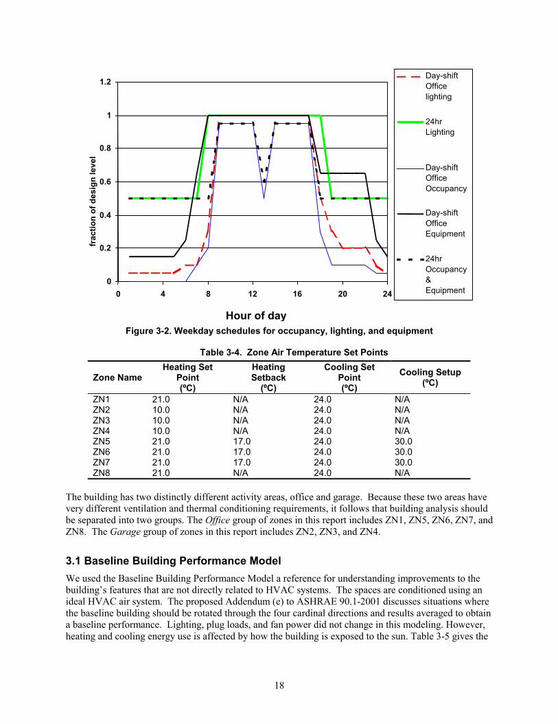
return air streams are not modeled. Real HVAC systems may meet the load using economizer cycles and heat recovery systems, thereby requiring much less energy than indicated by the Purchased Air models. (It would be better if ideal models were able to discount cooling needs during periods when free cooling is readily available.) Therefore, building performance baseline modeling is used for only part of the analysis where building fabric (envelope materials, glazing), form (skylights, clerestories, and overhangs) and operation (daylighting and certain ventilation schemes) are varied. Once the building has been optimized, HVAC systems are incorporated back into the models to determine energy use and energy costs relative to the Baseline Energy Model. An ideal HVAC air system is similar to a load calculation, but uses an annual weather file rather than design-day conditions. For this reason, we report peak heating and cooling loads and air mass flow rates to show how maximum equipment loading might vary for designs considered. Both the performance and energy baseline models are identical except for their HVAC systems. They have eight thermal zones (five office zones and three garage/maintenance zones as listed in Tables 3-1 and 3-2 and illustrated in Figure 3-1). The building envelope specifications, given in Table 3-3, correspond to the minimums provided in Table B-13 in ASHRAE Standard 90.1-2001. Table 3-3 also shows resulting performance levels computed by the EnergyPlus model because these are calculated from complete constructions (and are not given explicitly). Air ventilation requirements are per ASHRAE Standard 62-1999 (ASHRAE 1999) at 10 L/s·person for offices (following occupancy schedule) and 7.5 l/s·m2 for workshops (on at all times). No skylights are included in these models and no reductions for daylighting are provided. Internal loads from equipment (plug loads) were included, but they are subtracted from the subsequent total energy use when improvements are compared to the baseline. We determined schedules from the architectural program. Figure 3-2 shows selected weekday schedules, and Table 3-4 lists zone air temperature set points for cooling, heating, and setup/setback.
Table 3-1. Thermal Zone Description: Internal Gains Zone Name
Usage
Occupancy Schedule
Number of Occupants
Equipment Loads
(W)
LightingLoads
(W)
ZN1 CUSTOMS, OFFICE 24 HR 9 1600 4160 ZN2 SHOPS, GARAGE 24 HR 7 810 4050 ZN3 MAINTENANCE
GARAGE 24 HR 10 2970 14850
ZN4 ARFF GARAGE 24 HR 10 600 3000 ZN5 OFFICE 7 A.M.-10 P.M 20 6500 8450 ZN6 OFFICE 7 A.M -10
P.M. 15 3200 4160
ZN7 OFFICE 7 A.M -10 P.M.
20 6500 8450
ZN8 OFFICE 24 HR 15 3200 4160
Table 3-2. Thermal Zone Description: Geometry
Zone Name
Floor Area (m2)
Ceiling Height
(m)
Glazed Area (m2)
% Glazed Design
Ventilation (m3/s)
ZN1 297 3.962 142.8 61 0.09 ZN2 251 6.248 15.4 8 1.88 ZN3 920 7.467 94.8 18 6.90

17
ZN4 186 8.839 36.4 24 1.39 ZN5 604 4.267 101.7 43 0.20 ZN6 297 4.267 82.1 53 0.15 ZN7 597 4.572 111.8 41 0.20 ZN8 297 4.572 115.1 70 0.15
ZN2 ZN3
ZN4 ZN6
ZN5ZN1
ZN4 ZN8
ZN7
N Second Floor
Ground Floor Figure 3-1. Thermal zones used in design development models
Table 3-3. Envelope Specifications for Baseline Models per ASHRAE 90.1-2001 Envelope Component 90.1 Minimum
Requirements EnergyPlus As-Modeled
EXTERIOR WALLS (M2·K)/W RSI-2.3 RSI-2.73 BUILT-UP ROOF (M2·K)/W RSI-2.6 RSI-2.70 NORTH-FACING WINDOWS W/(M2·K)
USI – 3.24 SHGC – 0.49
USI – 3.14 SHGC – 0.488
OTHER-FACING WINDOWS W/(M2·K)
USI – 3.24 SHGC – 0.39
USI – 3.14 SHGC – 0.397
18
0
0.2
0.4
0.6
0.8
1
1.2
0 4 8 12 16 20 24
Hour of day
frac
tion
of d
esig
n le
vel
Day-shiftOffice lighting
24hr Lighting
Day-shiftOffice Occupancy
Day-shiftOffice Equipment
24hr Occupancy& Equipment
Figure 3-2. Weekday schedules for occupancy, lighting, and equipment
Table 3-4. Zone Air Temperature Set Points
Zone Name Heating Set
Point (ºC)
Heating Setback
(ºC)
Cooling Set Point (ºC)
Cooling Setup (ºC)
ZN1 21.0 N/A 24.0 N/A ZN2 10.0 N/A 24.0 N/A ZN3 10.0 N/A 24.0 N/A ZN4 10.0 N/A 24.0 N/A ZN5 21.0 17.0 24.0 30.0 ZN6 21.0 17.0 24.0 30.0 ZN7 21.0 17.0 24.0 30.0 ZN8 21.0 N/A 24.0 N/A
The building has two distinctly different activity areas, office and garage. Because these two areas have very different ventilation and thermal conditioning requirements, it follows that building analysis should be separated into two groups. The Office group of zones in this report includes ZN1, ZN5, ZN6, ZN7, and ZN8. The Garage group of zones in this report includes ZN2, ZN3, and ZN4.
3.1 Baseline Building Performance Model We used the Baseline Building Performance Model a reference for understanding improvements to the building’s features that are not directly related to HVAC systems. The spaces are conditioned using an ideal HVAC air system. The proposed Addendum (e) to ASHRAE 90.1-2001 discusses situations where the baseline building should be rotated through the four cardinal directions and results averaged to obtain a baseline performance. Lighting, plug loads, and fan power did not change in this modeling. However, heating and cooling energy use is affected by how the building is exposed to the sun. Table 3-5 gives the

19
results for the Baseline Building Performance Model. For actual energy use and costs, see Sections 3.2 and 3.3, respectively.
Table 3-5. Baseline Building Performance Model Results for Energy Use Zone
Group
Rotation (degree)
Lights (MWh/yr)
Equipment(MWh/yr)
Cooling(MWh/yr)
Heating(MWh/yr)
Total w/o Equipment (MWh/yr)
Intensity(kWh/ m2·yr)
0 133.5 24.2 0.0 318.6 452.1 333.1 90 133.5 24.2 0.0 314.9 448.4 330.4 180 133.5 24.2 0.0 305.0 438.5 323.1 270 133.5 24.2 0.0 315.2 448.7 330.7
GARAGES
AVERAGE 133.5 24.2 0.0 313.4 446.9 329.4 0 117.5 95.1 163.5 38.7 319.7 152.3 90 117.5 95.1 178.1 38.0 333.6 158.9 180 117.5 95.1 169.3 37.8 324.6 154.6 270 117.5 95.1 169.0 40.7 327.2 155.9
OFFICES
AVERAGE 117.5 95.1 170.0 38.8 326.2 155.4 The ideal HVAC air system also serves as an alternate method of sizing HVAC air systems. (The other method is to use automatic sizing models in energy programs like DOE-2.1E and EnergyPlus.) The drawback of using results from an ideal HVAC air system to size air handlers is that different capacities may be needed to overcome poor controlling and reheat situations in a real system. In addition, design-day conditions are probably more severe. However, EnergyPlus routines for automatically sizing HVAC systems can be problematic, leading to the desirability of using the quite robust models for the ideal Purchased Air systems to check sizing. Table 3-6 gives the loads that the air system must meet, by zone, for the unrotated baseline building performance model.
Table 3-6. Baseline Building Performance Model Results for Peak Loads Zone Name Peak heating
Load (W)
Peak Cooling Load (W)
Peak Air Mass Flow (kg/s)
ZN2 65,100 0 1.6 ZN3 241,000 0 5.92 ZN4 49,000 0 1.21 GARAGES COINCIDENT 355,000 0 8.73
ZN1 15,400 26,200 2.33 ZN5 16,100 30,400 2.70 ZN6 12,100 16,000 1.42 ZN7 25,000 35,500 3.15 ZN8 14,000 20,900 1.85 OFFICES COINCIDENT 73,100 121,000 10.7
3.2 Baseline Energy Model For the Baseline Energy Model, each office zone has its own packaged direct expansion (DX) cooling systems with outside air economizers. The COP is 3.2 for the smaller units and 3.1 for the larger ones. The garage and maintenance zones have similar systems but without cooling coils. These systems have

20
outdoor air mixers for supplying required ventilation air and implementing free cooling using an air-side economizer. Gas-fired heating coils provide heat for all the zones. Table 3-7 summarizes the results from rotating the Baseline Energy Model, where results have been combined separately for garage zones and office zones.
Table 3-7. Baseline Energy Model Results for Energy Use Rotation
(degree) Lights
(MWh/yr) Equipment(MWh/yr)
Fans (MWh/yr)
Cooling(MWh/yr)
Heating (MWh/yr)
Total w/o Equipment(MWh/y))
Intensity(kWh/ m2·yr)
0 133.5 24.2 78.8 0 326.6 538.9 397.1 90 133.5 24.2 78.8 0 322.4 534.7 394.1 180 133.5 24.2 78.8 0 310.3 522.6 385.1 270 133.5 24.2 78.8 0 322.6 534.9 394.2
Garages
AVERAGE 133.5 24.2 78.8 0 320.5 532.8 392.6 0 117.5 95.1 61.0 49.2 85.5 313.2 149.2 90 117.5 95.1 61.0 52.4 84.8 315.7 150.4 180 117.5 95.1 61.0 50.4 86.3 315.2 150.2 270 117.5 95.1 61.0 51.8 89.7 320.1 152.5
Offices
AVERAGE 117.5 95.1 61.0 51.0 86.6 316.1 150.6 The rotation study shows that simply rotating the building 180 degrees reduces heating energy in garage zones by 5% because there are more windows on the north side of the building. Going through the process of rotating and averaging results resulted in only a slight change (0.4%) to the Baseline Energy Model results (with plug loads removed). The unrotated energy usage for the entire building is 852.1 MWh/yr. After averaging four rotations, this changed to 848.9 MWh/yr.
3.3 Baseline Energy Costs Although levels of energy usage are important metrics, energy cost is another useful metric that can be used to compare dissimilar types of energy. Energy cost can also be factored into important economic analysis. Appendix D summarizes how we used simulation results from EnergyPlus to compute cost data for this analysis. We had to compute these data using an ancillary program because EnergyPlus does not offer the economic analysis. Table 3-8 lists the results for energy cost from the Baseline Energy Model. Total energy cost (with plug loads removed) for the entire baseline building per ASHRAE 90.1-2001(g), averaged for the four rotations, is $86,545/yr or $25.0 /m2·yr ($2.32 /ft2·yr).

21
Table 3-8. Baseline Energy Model Results for Energy Costs
Rotation (degree)
Lights ($/yr)
Equipment($/yr)
Fans($/yr)
Cooling($/yr)
Heating($/yr)
Total w/o Equipment
($/yr) Intensity($/m2·yr)
0 22,260 4,032 13,030 0 10,040 45,330 33.40 90 22,260 4,032 13,030 0 9,914 45,204 33.31 180 22,260 4,032 13,030 0 9,544 44,834 33.04 270 22,260 4,032 13,030 0 9,920 45,210 33.32
Garages
AVERAGE 22,260 4,032 13,030 0 9,854 45,144 33.27 0 19,770 15,930 10,060 8,598 2,629 41,057 19.56 90 19,770 15,930 10,060 9,162 2,609 41,601 19.82 180 19,770 15,930 10,060 8,813 2,654 41,297 19.67 270 19,770 15,930 10,060 9,059 2,760 41,649 19.84
Offices
AVERAGE 19,770 15,930 10,060 8,908 2,663 41,401 19.72
3.4 Baseline Thermal Comfort Occupant thermal comfort is the main goal of conditioning the interior spaces of buildings, making it useful to compare comfort as well as energy use and cost. Historically, energy analysis studies of design implications have focused on energy use and cost and have not necessarily quantified how energy efficient designs affect occupant thermal comfort. This can be justifiable in situations where space loads are being completely met by HVAC equipment because little difference in air temperatures would be expected. However, because the maintenance and garage spaces in this project are not cooled, there is a danger of designing a building for reduced heating energy and costs that subsequently overheats in the summer. Because no energy is used for cooling, energy analysis would not capture any strategies that help or hinder occupant comfort in these spaces during the summer. EnergyPlus yields results for several methods of predicting occupant thermal comfort. For this analysis, we selected the Fanger (1982) model for predicted mean vote (PMV) as implemented in EnergyPlus. PMV is in units of the ASHRAE Thermal Sensation Scale where +3 represents a “hot” sensation, +2 represents “warm,” +1 is “slightly warm,” 0 is “neutral,” –1 is “slightly cool,” –2 is “cool,” and –3 is “cold.” Hourly data for PMV are reduced to facilitate comparisons between different building models by summing the number of hours that PMV values are above or below certain thresholds. Table 3-9 presents results for the predictions of how occupants will sense garage spaces during the cooling season from the unrotated Baseline Building Performance Model.
Table 3-9. Summary of Baseline Performance Model Predictions for Occupant Thermal Comfort on ASHRAE Thermal Sensation Scale for Uncooled Garages and Shops
Zone Name Hours per Year Above +1.5
Hours per Year Above +2.0
Hours per Year Above +2.5
ZN2 445 75 9 ZN3 489 89 17 ZN4 550 121 20
More subtle reasons to quantify occupant thermal comfort arise because of arguments made in support of using building envelope components with high levels of thermal performance. Energy use and cost may not justify the highest levels of envelope thermal performance in commercial buildings where energy use characteristics are dominated by ventilation and internal loads. Therefore, comfort considerations are sometimes used to justify high-performance envelopes based on the economic benefits of worker

22
productivity and increased usability of perimeter floor space. During the winter, inside surface temperatures are warmer for envelope components with higher thermal performance. This leads to improved comfort because occupants exchange thermal radiation with envelope surfaces regardless of the air temperature. Comfort models capture this effect by incorporating radiant temperatures. (Other issues surrounding the inside surface temperatures, such as natural-convection-induced drafts and condensation, are not as easily considered.) In preparation for arguing that comfort issues warrant high-performance envelope materials, we reduced the hourly PMV results for the 24-hour office zones. Table 3-10 gives these results for the Baseline Building Performance Model.
Table 3-10. Summary of Baseline Building Performance Model Predictions for Occupant Thermal Comfort on ASHRAE Thermal Sensation Scale for Heating in 24-Hour Offices
Zone Name Hours per Year Below –0.4
Hours per Year Below –0.3
Hours per Year Below –0.2
ZN1 11 372 2051 ZN8 2 575 2614
The Baseline Energy Model may lead to different comfort conditions than those obtained with the Baseline Building Performance Model because HVAC system models and controls differ. Therefore, we also reduced comfort results for these models to arrive at a comfort baseline, which is given in Table 3-11. The garage zones are much less comfortable than the office zones because the heating set point is low and they are not actively cooled.
Table 3-11. Summary of Baseline Energy Model Predictions for Occupant Thermal Comfort on ASHRAE Thermal Sensation Scale for 24-Hour Office and Garage
Zone Name
Hours per Year
Below –2.0
Hours per Year
Below –1.0
Hours per Year
Below –0.5
Hours per Year
Above +0.5
Hours per Year
Above +1.0
Hours per Year
Above +2.0
ZN1 0 0 1332 3584 293 0 ZN3 3202 4639 5132 2229 1399 145

23
4.0 Elimination Parametric Study Using a customary approach where various factors are zeroed/negated in isolation, we performed a parametric analysis. This analysis differs from the one presented in Section 2.2 in that this analysis used the Baseline Energy Model, which corresponds to the Stage One proposed building rather than to a generic solar-neutral office building. Because of the significant differences between the office-type and garage-type zones, we split the study presented in this section into two groups with separate baseline performance levels for each. Table 4-1 summarizes how the different measures would rate compared to the ASHRAE 90.1-2001(e) baseline (where plug loads are removed).
Table 4-1. Summary of Baseline Parametric Study by Type of Zone Case
Garage Zones
% Change Office Zones
% change R-100 WALLS –1.2 –2.2 R-100 ROOF –2.5 –6.3 R-100 FLOOR +3.3 +0.8 U-0.01 GLAZING –0.7 –6.7 ALL R-100/U-0.01 –1.2 –13.1 NO SOLAR GLAZING +0.46 +1.9 NO LIGHTS –14.5 –31.3 NO PEOPLE +1.4 +1.0 NO EQUIPMENT +1.9 +3.7 NO OS AIR –60.6 –11.9 NO INFILTRATION –0.03 –4.5
The results show that envelope improvements offer only minor improvements in energy efficiency and that lighting and outdoor air ventilation are important. See Appendix F for additional results of a parametric elimination study where results for the entire building are presented together and compared to earlier simulations using the DOE-2.1E computer program.

24
5.0 Improved Energy Designs In this section, we present energy simulation results for improvements to the baseline building. The starting point is the proposed Stage One, Scheme A-2 building plan built to meet ASHRAE 90.1-2001 and modeled according to proposed informational Appendix (g). The baseline modeling (see Section 3.0) yields metrics for evaluating if the goal of reducing energy costs by 50% has been met. The elimination modeling (see Section 4.0) furnishes guidance on where to place focus when developing energy efficient designs. Quantitative predictions for how design measures will affect energy use are made possible through the extensive use of energy simulation. Although we recognize that whole-building analysis achieves the best results, it is useful to proceed in a step-by-step manner to organize documentation and gain insight into complex integration issues. This section presents the development of an improved energy efficient design (and EnergyPlus models and results) in the following stages and subsections:
1. Envelope Improvements—Section 5.1 2. Daylighting with Skylights—Section 5.2 3. Daylighting with Clerestories and Overhangs—Section 5.3 4. Demand-Controlled Ventilation—Section 5.4 5. HVAC systems—Section 5.5.
See Section 7.0 for a discussion of the results and Section 8.0 for design recommendations based on those results. In general, such a study should also investigate modifications of the overall shape and layout, or “massing,” of the building. However, no major reconfigurations of the floor plan were made for this building because it had already been elongated and given an advantageous east–west orientation (perhaps in response to predesign analysis). In addition, extensive efforts to do additional massing studies are not warranted at this time because the Teterboro Airport Building is currently on hold and its architectural program is expected to change.
5.1 Envelope Constructions Increasing levels of thermal insulation and using glazing with improved thermal and optical properties are often the first and relatively simple methods used to improve the energy efficiency of a building. However, the relatively high levels of envelope thermal performance specified in ASHRAE 90.1-2001 make this measure less effective than when less stringent standards are followed. The elimination parametric study shows that even outrageous levels of thermal performance would have relatively minor effects on overall energy use. Nevertheless, the highest performance buildings will tend to use envelope components with levels of thermal performance that exceed code. Wall and roof construction assemblies recommended by the architect appear adequate and were used in the “Improved Envelope Model.” This exterior wall construction includes a metal panel rain screen, rigid foam insulation, cellulose cavity insulation, and gypsum wallboard. We selected glazing for the modeling based on Viracon’s Azurlite, but with a low-emittance coating in argon-filled, insulating glazing units. We modeled a second version of envelope modifications called “High-Mass Envelope” with tiled floors and slabs instead of carpet and exterior walls with concrete block adjacent to interior wall board and insulation on the outside. The interior walls were symmetric, composed of double layers of concrete block walls with a layer of foam insulation between them. Table 5-1 gives the performance levels of envelope components (as computed by EnergyPlus).

25
The floor slab was not insulated underneath because model results showed that ground contact is beneficial. Vertical insulation should be installed around the perimeter of the slab as required in ASHRAE 90.1-2001. Note that ground temperature calculations were based on the presence of such insulation, but the whole building models do not account for vertical perimeter slab insulation. These results depend on the ground temperatures modeled by the preprocessor (slab.exe, provided with EnergyPlus) where temperatures were found to stay around 20°C.
Table 5-1. Envelope Thermal Performance Levels
Item Baseline Model
Improved Envelope
Model High-Mass Envelope
EXTERIOR WALL CONDUCTANCE (W/M2·K) 0.3664 0.2881 0.4067 INTERIOR WALL CONDUCTANCE (W/M2·K) 0.4088 0.4088 0.5064 ROOF CONDUCTANCE (W/M2·K) 0.3701 0.1939 0.1939 SLAB + 0.3 M DIRT CONDUCTANCE (W/M2·K) 0.5217 0.5217 0.5217
CARPETED SLAB + 0.3 M DIRT CONDUCTANCE (W/M2·K) 0.4687 0.4687 0.5191
(TILED)
INTERIOR FLOOR CONDUCTANCE (W/M2·K) 0.6599 0.3046 0.3252 (TILED)
NORTH GLAZING CONDUCTANCE (W/M2·K) 3.139 1.479 1.479 NORTH GLAZING SHGC 0.488 0.175 0.175 NON-NORTH GLAZING CONDUCTANCE (W/M2·K) 3.138 1.479 1.479
NON-NORTH GLAZING SHGC 0.397 0.175 0.175 Table 5-2 summarizes results for energy use and peak load conditions, and Tables 5-3 and 5-4 give the occupant thermal comfort results.
Table 5-2. Summary of Results for Energy Use and Peak Loads: Envelope Change Models Garages Offices
Baseline Rot. 0 (unrotated)
Improved Envelope
High- Mass Baseline Improved
Envelope High- Mass
IDEAL HEATING ENERGY (MWH/YR) 318.6 309.7
(–2.8%) 307.6 (–3.5%) 38.7 9.8
(–74.7%) 8.4 (–78.3%)
IDEAL COOLING ENERGY (MWH/YR) 0 0.0 0.0 163.5 140.0
(–14.4%) 131.6 (–19.5%)
PEAK HEATING LOAD (W) 355,000 345,000
(–2.8%) 343,000 (–3.4%) 73,100 39,300
(–46.2%) 46,100 (–36.9%)
PEAK COOLING LOAD (W) 0.0 0.0 0.0 121,00 89,100
(–26.4%) 84,300 (–30.3%)
PEAK AIR MASS FLOW RATE (KG/S)
8.73 8.50 8.43 10.7 7.91 7.49

26
Table 5-3. Summary of Occupant Thermal Comfort Predictions on ASHRAE Thermal
Sensation Scale for Uncooled Garages and Shops: Envelope Change Models Zone Name
Scenario Hours per Year Above 1.5
Hours per Year Above 2.0
Hours per Year Above 2.5
BASELINE 445 75 9 IMPROVED ENVELOPE
396 67 5 ZN2
HIGH-MASS 271 27 0 BASELINE 489 89 17 IMPROVED ENVELOPE
399 67 7 ZN3
HIGH-MASS 321 38 0 BASELINE 550 121 20 IMPROVED ENVELOPE
430 72 8 ZN4
HIGH-MASS 282 27 0
Table 5-4. Summary of Occupant Thermal Comfort Predictions on ASHRAE Thermal Sensation Scale for Heating in 24-Hour Offices: Envelope Change Models
Zone Name
Scenario Hours per Year Below –0.4
Hours per Year Below –0.3
Hours per Year Below –0.2
BASELINE 11 372 2051 IMPROVED ENVELOPE
0 49 871 ZN1
HIGH-MASS 0 64 911 BASELINE 2 575 2614 IMPROVED ENVELOPE
0 69 1402 ZN8
HIGH-MASS 0 87 1471
5.2 Daylighting with Skylights This section presents an analysis of daylighting opportunity without altering the geometry of the building enclosure. Lighting controls are implemented that dim electric lights in response to the availability of daylight in the spaces. In this section the overall shape of the enclosure is not altered but flush-mounted, and horizontal skylights are added to allow daylight into the building. In Section 5.3, we further develop daylighting opportunities using overhangs and clerestories that do alter the shape of the building envelope. Skylights were installed horizontally in the roof as shown in Figure 5-1. The figure also shows where the table-height daylight control sensors were placed in the zones. The rows of skylights in the east end of the building are located over an atrium open to ZN5 and ZN7. The floor and ceiling surfaces separating ZN5 and ZN7 were shortened to allow daylight to enter ZN5. The northern row of skylights was associated with ZN5, located on the first floor, underneath ZN7. The skylights use double-pane insulated glazing units with a low-e coating and argon gas fill. The low-e coating is also on a glazing layer with a composition tint (Azurlite).

27
Skylights added to building for daylighting
Daylight sensor locations
ZN5
Figure 5-1. Roof plan: skylight layout
Implementing daylighting implies that electric lights are controlled to turn off when they are not needed. Table 5-5 lists the design lighting energy levels and fractions that we assumed to be dimmable for the daylighting models in this report. Table 5-6 summarizes energy-related results from the daylighting modeling with the added skylights. Table 5-7 gives the results for thermal comfort in the garage spaces, and Table 5-8 presents the results for thermal comfort in the 24-hour office spaces.
Table 5-5. Modeling of Lighting Controls for Daylighting
Zone Name Design Power Level(W) Fraction Replaceable Illuminance Threshold Set Point
(lux) ZN1 4160 0.8 500 ZN2 4050 1.0 500 ZN3 14850 1.0 500 ZN4 3000 1.0 500 ZN5 8450 0.8 500 ZN6 4160 0.8 500 ZN7 8450 0.8 500 ZN8 4160 0.9 500
Table 5-6. Summary of Results for Energy Use and Peak Loads: Daylighting with Skylights Models
Garages Offices Baseline Daylighting with
Skylights % Baseline Daylighting with Skylights %
IDEAL HEATING ENERGY (MWH/YR) 318.6 336.1 +5.5 38.7 19.5 –49.6
IDEAL COOLING ENERGY (MWH/YR) 0 0.0 163.5 89.1 –45.5
LIGHTING ELECTRICITY (MWH/YR)
133.5 50.6 –62.1 117.5 69.1 –41.2
PEAK HEATING LOAD (W) 355,000 354,000 –0.3 73,100 56,000 –23.4
PEAK COOLING LOAD (W) 0.0 0 121,00 72,800 –39.8

28
PEAK AIR MASS FLOW RATE (KG/S)
8.73 8.72 0.1 10.6 6.46 –39.1
Table 5-7. Summary of Occupant Thermal Comfort Predictions on ASHRAE Thermal Sensation Scale for Uncooled Garages and Shops: Daylighting with Skylights Model
Zone Name
Scenario Hours per Year Above 1.5
Hours per Year Above 2.0
Hours per Year Above 2.5
BASELINE 445 75 9 ZN2 DAYLIGHTING WITH
SKYLIGHTS 250 35 0
BASELINE 489 89 17 ZN3 DAYLIGHTING WITH
SKYLIGHTS 260 40 0
BASELINE 550 121 20 ZN4 DAYLIGHTING WITH
SKYLIGHTS 297 44 0
Table 5-8. Summary of Occupant Thermal Comfort Predictions on ASHRAE Thermal Sensation Scale for Heating in 24-Hour Offices: Daylighting with Skylights Model
Zone Name Scenario Hours per Year Below
–0.4
Hours per Year Below –0.3
Hours per Year Below –0.2
BASELINE 11 372 2051 ZN1 DAYLIGHTING
WITH SKYLIGHTS 0 51 1047
BASELINE 2 575 2614 ZN 8 DAYLIGHTING
WITH SKYLIGHTS 0 83 1597
5.3 Overhangs and Clerestories Here we present results from models incorporating passive solar and daylighting strategies that use overhangs and clerestories. Overhangs are a well-known method of providing seasonally dependent shading and, therefore, solar heat gain. Modern glazing technologies offer products with low solar heat gain characteristics, quantified by the SHGC, that give the appearance of providing design solutions for reducing unwanted solar heat without overhangs. However, low-SHGC glazing does not guarantee that solar heat entering the building will not be excessive. The glazing means only that direct solar gains will be reduced by some percent. Overhangs can block that direct gain. Furthermore, low-SHGC glazing layers may absorb considerable solar heat, causing their interior surfaces to become warm, which leads to possible problems with occupant thermal comfort. Occupants sitting in direct sun are always likely to be uncomfortable. In buildings with heating load, such as the maintenance and garage areas for the Teterboro airport building, low-SHGC glazing will reduce solar heat gains that are actually desirable during the winter. A building that is designed to be sensitive to climate will allow heat gains in the winter but not in the summer, and overhangs on south-facing windows with high-SHGC windows are a good design solution.

29
The latitude of the location can be used to determine appropriate dimensions for overhang design. Figure 5-2 shows recommended ratios for designing overhangs for windows facing south in Newark, New Jersey (Marion and Wilcox 1995). We used these ratios to design overhangs for south-facing windows in the energy simulations developed in this section.
0.554
0.32
41.
000Window
Vertical Gap
Overhang
Figure 5-2. South-facing overhang design ratios, latitude 40.70 N
To obtain good passive solar heating for zones that require significant heating, we increased south-facing glazing areas for garage zones and added overhangs to all south-facing glazing areas. Although offices still require cooling (after the morning warm-up), the garage and maintenance areas have high ventilation rates and low equipment loads. This makes using passive solar heating to meet heating loads desirable. The south-facing windows in these zones can use high-SHGC glazing (SHGC = 0.55) as long as they are shaded from direct gains during the cooling season. Figure 5-3 diagrams the model with overhangs and clerestories. We added a long upper window and overhang to the southern exposure of the central garage area of ZN3, and altered the roofs of ZN2 and ZN3 to create large clerestories with south-facing glazing using crude sawtooth-shaped rooflines. Low-SHGC glazing (SHGC = 0.175) remains in use on office zones. Lighting levels and controls, given in Table 5-5, are the same as for the skylights.

30
Skylights added to building for daylighting
Daylight sensor locations
Overhang added to south-facing windows
Sawtooth clerestories added to roof
Southwest Isometric veiw
Roof plan schematic
Figure 5-3. Clerestory and overhang layout
For the office zones, passive solar heating is not desirable because cooling is needed throughout the “heating” season. But because daylighting is advantageous, we added a north-facing clerestory above an atrium running along the center of the east end of the building office areas. A south-facing clerestory could be designed with overhangs to protect from direct solar gains, but north views may be desirable for this building because the airfield is that direction. A north-facing clerestory does not need an overhang.

31
Figure 5-4 diagrams the north-facing clerestory and depicts how the atrium is modeled. EnergyPlus requires a one-to-one association between windows and zones for daylight calculations (but not solar thermal calculations). The clerestory glazing was subdivided and associated with different zones, as shown in Figure 5-4.
ZN7
ZN5
ZN8
ZN6
ZN7
ZN5
ZN8
ZN6
Front View (from North) of Clerestory Glazing Layout
ZN5 ZN6
ZN8ZN7
Diffuse lightfrom north
Section View (from East) of Zones and Clerestory
Figure 5-4. Atrium modeling for daylighting
Results for energy usage and peak system loads are given in Table 5-9, and Tables 5-10 and 5-11 show the results for predicted comfort levels.

32
Table 5-9. Summary of Results for Energy Use and Peak Loads: Overhangs and
Clerestories Model Garages Offices Baseline Overhangs and
Clerestories % Baseline Overhangs and
Clerestories %
IDEAL HEATING ENERGY (MWH/YR) 318.6 313.6 –1.6 38.7 21.7 –43.9
IDEAL COOLING ENERGY (MWH/YR) 0 0 163.5 73.5 –55.0
LIGHTING ELECTRICITY (MWH/YR)
133.5 64.6 –51.6 117.5 57.9 –50.7
PEAK HEATING LOAD (W) 355,000 346,000 –2.5 73,100 55,600 –23.9
PEAK COOLING LOAD (W)
0.0 0 121,00 65,200 –46.1
PEAK AIR MASS FLOW RATE (KG/S)
8.73 8.52 –2.4 10.7 5.78 –46.0
Table 5-10. Summary of Occupant Thermal Comfort Predictions on ASHRAE Thermal Sensation Scale for Uncooled Garages and Shops: Overhangs and Clerestories Model
Zone Name Scenario
Hours per Year Above
1.5
Hours per Year Above
2.0 Hours per Year
Above 2.5
BASELINE 445 75 9 ZN2 OVERHANGS AND
CLERESTORIES 334 46 0
BASELINE 489 89 17 ZN3 OVERHANGS AND
CLERESTORIES 311 46 0
BASELINE 550 121 20 ZN4 OVERHANGS AND
CLERESTORIES 299 44 0

33
Table 5-11. Summary of Occupant Thermal Comfort Predictions on ASHRAE Thermal
Sensation Scale for Heating in 24-Hour Offices: Overhangs and Clerestories Model
Zone Name Scenario
Hours per Year Below
–0.4
Hours per Year Below –0.3
Hours per Year Below –0.2
BASELINE 11 373 2051 ZN1 OVERHANGS AND
CLERESTORIES 0 47 1032
BASELINE 2 572 2604 ZN8 OVERHANGS AND
CLERESTORIES 0 132 2213
5.4 Demand-Controlled Ventilation ASHRAE Standard 62-1999 (ASHRAE 1999) specifies ventilation requirements for commercial buildings. The prescriptive requirements for the garage/maintenance areas of the Teterboro Airport building are assumed to correspond to those of an automotive workshop at 7.5 L/s·m2. This is a great deal of outdoor ventilation air that must be heated during winter months, using considerable fan power. As with other standards, ASHRAE 62-1999 allows for two methods of meeting requirements, a performance method and a prescriptive method. The prescriptive method in this case is maintaining a constant minimum ventilation rate at all times (because these areas operate 24 hours). Although the prescriptive method should ensure adequate indoor air quality (IAQ) in a well-mixed zone, it entails considerable energy use. To meet the energy performance goals and ensure good IAQ, we recommend a performance method for ventilation. In this method, sensors are used to continuously monitor IAQ and adjust ventilation rates as needed. In addition, air delivery should be of the type known as “displacement ventilation,” where fresh air is introduced low to the ground and subsequently leaves the space at or near the ceiling. This technique avoids complete mixing and results in good IAQ in industrial spaces. Displacement ventilation cannot be modeled well in current whole-building energy simulation programs. With detailed information on the configuration of sources of heat and pollutants, the effectiveness of displacement ventilation designs could be further analyzed with computational fluid dynamics. However, we present no further analysis of displacement ventilation in this report. Incorporating sensors to control ventilation rates is referred to as “demand-controlled ventilation.” With sensors to detect CO2, carbon monoxide, volatile organic compounds, and particulates, for example, the ventilation rates will vary depending on the activities occurring in the garages and shops. Because these activities and sources of air pollutants are not yet known for this specific project, we made the following assumptions to allow the energy implications of demand-controlled ventilation to be modeled at this early stage of the design process:
• Pollutant production varies directly with occupancy rates. • Pollutant production is uniformly random. • A minimum threshold of 25% of the prescriptive level of ventilation air is appropriate.
Based on these assumptions, we formulated new schedules for controlling the rates of introducing outdoor air into the garage and shop zones (ZN2, ZN3, and ZN4). Each zone is given a schedule for ventilation rates for every hour of the year based on Equation 5-1. The schedule yields a value for the fraction of

34
design level that is to be used for a given hour. This design outdoor air rate is the prescriptive amount of ventilation air from ASHRAE 62-1999.
[ ]iuiOCCPiOA rfMAXf ,,, ,25.0 ∗= Eq. 5-1
where iOAf , is the fraction of design outdoor air at hour i
iOCCPf , is the fraction of design occupancy at hour i
iur , is the uniform pseudorandom number on [0..1] for hour i i is hour of year. [ ],MAX is the operator selecting higher of two parameters We generated three independent, randomized schedules for the garage-type zones and added them to the model from Section 5.3 (overhangs and clerestories). This new model is termed “Demand-Controlled Ventilation.” Table 5-12 summarizes the energy and load results for this model, and comfort results are summarized in Table 5-13.
Table 5-12. Summary of Results for Energy and Load in Demand-Controlled
Garage/Shop/ARFF Spaces
Baseline Demand-
Controlled Ventilation
% Change
IDEAL HEATING ENERGY (MWH/YR) 318.6 69.2 –78.3
PEAK HEATING LOAD (W) 355,000 258,000 –27.3
PEAK AIR MASS FLOW RATE (KG/S) 8.73 6.35 –27.3
Table 5-13. Summary of Predictions for Occupant Thermal Comfort on ASHRAE Thermal Sensation Scale for Uncooled Garages and Shops: Demand-Controlled Ventilation and
Baseline Performance Model Zone Name Model Hours per Year
Above 1.5 Hours per Year
Above 2.0 Hours per Year
Above 2.5 BASELINE 445 75 9
ZN2 DEMAND-CONTROLLED VENTILATION 638 82 1
BASELINE 489 89 17 ZN3 DEMAND-CONTROLLED
VENTILATION 517 57 0
BASELINE 550 121 20 ZN4 DEMAND-CONTROLLED
VENTILATION 500 52 0

35
5.5 HVAC Systems This section presents modeling results where we specified HVAC systems so that we can predict the building’s energy use and cost. The first subsection focuses on office zones that are conditioned using rooftop-packaged units, and the second subsection discusses heating and ventilating garage zones.
5.5.1 Office Zone DX Equipment Rooftop-packaged units offer economic advantages for smaller commercial buildings. The units we considered here are mid-sized industrial rooftop-packaged units with cooling provided by DX cooling coils. The Baseline Energy Model presented in Section 3.0 uses five separate constant-volume, rooftop- packaged units, one for each zone. This system serves as a starting point. EnergyPlus allows performance details of particular HVAC systems and components to be specified. More often than not, DX equipment is operating under conditions that differ from conditions under which the equipment was rated. EnergyPlus allows using performance curves that are input explicitly rather than relying on defaults hard-coded into the program’s models. Each DX cooling coil uses four performance curves and a fifth part-load curve. Because equipment-specific data for generating part-load curve are difficult to obtain, we used a single curve recommended by a manufacturer for a separate modeling exercise (Neymark and Judkoff 2002) for all of the DX system models. Two of the performance curves are biquadratic curves, one for capacity and one for energy input ratio (EIR), as a function of two different air temperatures, one entering the evaporator and the other entering the condenser. EIR is the inverse of COP. The other two performance curves are second-order quadratic curves for capacity and EIR, as a function of airflow rate through the coil. The performance curves were generated from manufacturer performance data tables (Carrier Corporation, Syracuse, New York; 2002) using function-fitting routines from a commercial mathematics program (Wolfram 1999). The curves are documented and available in the EnergyPlus input files. See Appendix E for more information on how we generated the performance curves. The first step in developing energy use and cost results is to attach the same DX system used in the Baseline Energy Model to the building form, function, and fabric developed through the Overhangs and Clerestories Model discussed in Section 5.3. This model includes envelope improvements, daylighting via clerestories, and overhangs over south-facing glazing. All four of the modeling steps in this section use this building description with different HVAC systems. Table 5-14 shows energy use and Table 5-15 presents energy cost results for these simulations. Table 5-16 compares comfort predictions for the different systems.
Table 5-14. Summary of Results for Energy Use for Office Zones with Constant-Volume DX Rooftop-Packaged Units
Lights (MWh/yr)
Equipment (MWh/yr)
Fans (MWh/yr)
Cooling(MWh/yr)
Heating(MWh/yr)
Total w/o equipment (MWh/yr)
Intensity(kWh/ m2·yr)
BASELINE AVERAGE 117.5 95.1 61.0 51.0 86.6 316.1 150.6
OVERSIZED DX 57.9 95.1 61.0 33.3 (–34.7%)
58.8 (–32.1%)
211.1 (–33.2%) 100.6
DOWNSIZED DX 57.9 95.1 35.3 29.7 (–41.8%)
75.1 (–13.3%)
198.0 (–37.4%) 94.3
DOWNSIZED DX + HRV* 57.9 95.1 35.3 30.5
(–40.2%) 26.4 (–69.5%)
150.1 (–52.5%) 71.5
HIGH-EFFICIENCY DOWNSIZED DX + HRV*
57.9 95.1 35.3 23.1 (–54.7%)
12.6 (–85.5%)
129 (–59.2%) 61.4
*HRV: heat recovery ventilators.

36
Table 5-15. Summary of Results for Energy Cost for Office Zones with Constant-Volume DX Rooftop-Packaged Units
Lights ($/yr)
Equipment($/yr)
Fans($/yr)
Cooling($/yr)
Heating($/yr)
Total w/o Equipment
($/yr) Intensity($/m2·yr)
BASELINE AVERAGE 19,770 15,934 10,065 8,565 2,588 40,983 19.72
OVERSIZED DX 9,577 15,934 10,065 5,821 1,809 27,267 (–33.5%) 12.99
DOWNSIZED DX 9,577 15,934 5,827 5,185 2,309 22,898 (–44.1%) 10.91
DOWNSIZED DX + HRV 9,577 15,934 5,827 5,314 812 21,530 (–47.5%) 10.26
HIGH-EFFICIENCY DOWNSIZED DX + HRV 9,577 15,934 5,827 4,069 812 20,285
(–-50.5%) 9.66
The Oversized DX Model uses the same DX equipment as the Baseline Energy Model except that the DX coil models were based on actual 90.1-compliant products. For the Baseline Energy Model, we used the lower rated COPs of 3.1 and 3.2 as the specified minimums from 90.1-2001(g). For the standard-efficiency systems, we selected specific units (Carrier models 48TM008 and 48TM014) that have rated COPs of 3.76 and 3.48, respectively. The capacity and efficiency performance curves in the Baseline Energy Model were those that correspond to these specific models. The standard-efficiency DX units were suitable for the Baseline Energy Model but become “oversized” once other building improvements are made. The Downsized DX Model uses smaller, standard-efficiency DX equipment based on the results of separate, design-day sizing simulations using EnergyPlus. The improved envelope and daylighting controls allow the size of installed HVAC equipment to be reduced. The sizing runs (not presented) showed that the two nominal 14-ton units can be replaced with 12-ton units and the three nominal 7-1/2- ton units could be replaced by 4-ton units. We selected specific downsized DX units (Carrier models 48TM005 and 48TM012) with rated COPs of 3.2 and 3.76, respectively. Capacity and efficiency curves were changed as well to match published performance data for these systems. The Downsized DX + HRV Model uses the same DX equipment but adds heat recovery equipment to the outdoor air system. The recovery systems are modeled as 62% effective, counterflow, flat-plate, air-to-air heat exchangers. These heat exchangers exchange only sensible heat and are always on. (No enthalpy wheel models are currently available in EnergyPlus). The High-Efficiency Downsized DX + HRV Model uses the same configuration as the previous model, but replaces the standard-efficiency DX equipment with higher efficiency equipment. We selected specific new DX units (Carrier models 48HJ005 and 48HJ012) with rated COPs of 3.92 and 3.97, respectively. Capacity and efficiency curves were changed as well to match published performance data for these systems.
Table 5-16. Summary of Predictions for Occupant Thermal Comfort on ASHRAE Thermal Sensation Scale for 24-Hour Office: ZN1
Model Hours per
Year Below –1.0
Hours per Year Below
–0.5
Hours per Year Above
+0.5
Hours per Year Above
+1.0
Hours per Year Above
+2.0 BASELINE 0 1332 3584 293 0 OVERSIZED DX 0 269 3261 0 0
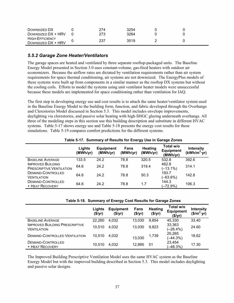
37
DOWNSIZED DX 0 274 3254 0 0 DOWNSIZED DX + HRV 0 273 3264 0 0 HIGH-EFFICIENCY DOWNSIZED DX + HRV 0 237 3519 2 0
5.5.2 Garage Zone Heater/Ventilators The garage spaces are heated and ventilated by three separate rooftop-packaged units. The Baseline Energy Model presented in Section 3.0 uses constant-volume, gas-fired heaters with outdoor air economizers. Because the airflow rates are dictated by ventilation requirements rather than air system requirements for space thermal conditioning, air systems are not downsized. The EnergyPlus models of these systems were built up from components in a similar manner as the rooftop DX systems but without the cooling coils. Efforts to model the systems using unit ventilator heater models were unsuccessful because these models are implemented for space conditioning rather than ventilation for IAQ. The first step in developing energy use and cost results is to attach the same heater/ventilator system used in the Baseline Energy Model to the building form, function, and fabric developed through the Overhangs and Clerestories Model discussed in Section 5.3. This model includes envelope improvements, daylighting via clerestories, and passive solar heating with high-SHGC glazing underneath overhangs. All three of the modeling steps in this section use this building description and substitute in different HVAC systems. Table 5-17 shows energy use and Table 5-18 presents the energy cost results for these simulations. Table 5-19 compares comfort predictions for the different systems.
Table 5-17. Summary of Results for Energy Use in Garage Zones
Lights (MWh/yr)
Equipment (MWh/yr)
Fans (MWh/yr)
Heating(MWh/yr)
Total w/o Equipment (MWh/yr)
Intensity (kWh/m2·yr)
BASELINE AVERAGE 133.5 24.2 78.8 320.5 532.8 392.6 IMPROVED BUILDING PRESCRIPTIVE VENTILATION 64.6 24.2 78.8 319.4 462.8
(–13.1%) 314.1
DEMAND-CONTROLLED VENTILATION 64.6 24.2 78.8 50.3 193.7
(–63.6%) 142.8
DEMAND-CONTROLLED + HEAT RECOVERY 64.6 24.2 78.8 1.7 144.3
(–72.9%) 106.3
Table 5-18. Summary of Energy Cost Results for Garage Zones
Lights($/yr)
Equipment ($/yr)
Fans ($/yr)
Heating($/yr)
Total w/o Equipment
($/yr) Intensity($/m2·yr)
BASELINE AVERAGE 22,260 4,032 13,030 9,854 45,330 33.40 IMPROVED BUILDING PRESCRIPTIVE VENTILATION 10,510 4,032 13,030 9,823 33,363
(–26.4%) 24.60
DEMAND-CONTROLLED VENTILATION 10,510 4,032 13,030 1,739 25,265
(–44.3%) 18.62
DEMAND-CONTROLLED + HEAT RECOVERY 10,510 4,032 12,895 51 23,454
(–48.3%) 17.30
The Improved Building Prescriptive Ventilation Model uses the same HVAC system as the Baseline Energy Model but with the improved building described in Section 5.3. This model includes daylighting and passive solar designs.

38
The Demand-Controlled Ventilation Model uses the same HVAC system but reduces outdoor ventilation rates in an effort to simulate how a sensor-based ventilation system might perform, as discussed in Section 5.4. The Demand-Controlled + HRV Model adds air-to-air heat recovery ventilation equipment. These systems are modeled as 62% effective, counterflow, flat-plate, air-to-air heat exchangers. These heat exchangers exchange only sensible heat, and have much larger nominal flow rates than the units for the offices.
Table 5-19. Summary of Predictions for Occupant Thermal Comfort on ASHRAE Thermal
Sensation Scale for 24-Hour Garages: ZN3
Model Hours per
Year Below –2.0
Hours per Year
Below –1.0
Hours per Year
Below –0.5
Hours per Year
Above +0.5
Hours per Year
Above +1.0
Hours per Year
Above +2.0
BASELINE 3202 4639 5132 2229 1399 145 IMPROVED BUILDING PRESCRIPTIVE VENTILATION
3114 4643 5167 2051 1202 71
DEMAND-CONTROLLED VENTILATION 3119 4641 5144 2423 1765 195
DEMAND- CONTROLLED + HEAT RECOVERY 2162 4438 4733 3501 3317 1483

39
6.0 Renewable Electricity Production Generating electricity using clean, renewable solar electric panels may be desirable for this project. This section presents an analysis of the amount of electricity that could be produced by a photovoltaic (PV) system at the Teterboro site.
6.1 Photovoltaic Modeling in PVSyst We predicted the annual energy production from a PV system for the Teterboro site using a model of the entire PV system with the simulation program PVSYST Version 3.2 (Mermond 2002). Inputs to this model include PV panel size and manufacturer, array wiring configuration and associated losses, array tilt and azimuth, hourly weather data, and inverter size and type. The model also simulates system-specific inputs, such as isolation transformer losses and array wiring losses. The PV system modeled in PVSyst was a 20-kWp, 3-phase grid-tied system with no battery storage. The modules used for this system were monocrystalline BP Solar 80-Wp panels (BP Solar, Linthicum, Maryland; 2001). With 16 modules in series and 16 strings in parallel, the entire array is rated at 20.5-kWp (393 volts direct current [DC] and 81 amps) at the peak output under standard test conditions. An 18-kW, grid-tied, inverter was selected along with an energy efficient isolation transformer. This inverter/transformer model includes a maximum power point tracker and the 97% efficient isolation transformer. Figure 6-1 is a diagram of the proposed system.
Building Loads
PV Array
400 VDC 80A
208/120 VAC 3-Phase
INVERTER Isolation
Transformer
PV ACDisconnect
and AC CircuitBreakers
Utility Grid
MAIN
DISTRIBUTION
PANEL
MDP
Figure 6-1. 20-kWp PV system schematic
This PV model includes associated system losses that are summarized in Figure 6-2. At an insolation level of 800 W/m2 and an ambient temperature of 20°C, the largest system degradation from theoretical results from module thermal losses. Under these operating conditions, the model predicts cell temperatures of 45°C. As the cell temperature increases, the module output decreases. These thermal losses are 9.3% of the theoretical maximum.

40
Figure 6-2. Current-voltage curves of system losses and performance at expected environmental
conditions
Typical meteorological year (TMY) weather data for New York City (Newark would have been a better choice because the building is closer to it, but the building location is almost between the two cities.) were used to model the expected annual performance. To determine the optimal angle, we simulated the described PV system at an azimuth of 0.0 (array facing south) and at varying tilt angles. As shown in Figure 6-3, the annual alternating current (AC) PV output is plotted versus a range of tilt angles from 0.0° to 90.0°. The results indicate that the optimal tilt angle is 32°. At this angle, the PV system is predicted to produce 26,285 kWh/yr. For tilt angles between 10° and 50°, the annual performance is degraded by less than 6.0% as compared to the optimal tilt performance. Table 6-1 summarizes the monthly performance at an array tilt of 32° for a 20-kWp PV system. The difference in seasonal insolation is the primary reason for an optimal array tilt that is less than the site latitude. As shown in Figure 6-4, the distribution of insolation for the summer months between the equinoxes is at higher bins of global horizontal insolation, and the total insolation distribution for the winter months between the equinoxes is at the lower end of the insolation bins. Because the summer months have higher solar altitude angles, the PV array tilt is optimized to take full advantage of the high summer insolation by reducing tilt to 32° from the latitude tilt of 41°.

41
0
5,000
10,000
15,000
20,000
25,000
30,000
0 10 20 30 40 50 60 70 80 90 100PV Array Tilt
Ann
ual A
C P
V Pr
oduc
tion
(kW
h)
0
10
20
30
40
50
60
Deg
rada
tion
Perc
ent
Annual AC OutputPercent Degradation from Optimal
Figure 6-3. PV array tilt optimization
Table 6-1. Summary of Predicted PV Performance by Month: 32° Tilt
Total Horizontal Insolation (kWh/m2)
Total Insolation on Collector (kWh/m2)
DC PV Energy (kWh)
AC PVEnergy (kWh)
System Conversion Efficiency
(%) JANUARY 58 87.2 1686 1553 11.1 FEBRUARY 76 100.5 1945 1794 11.1 MARCH 116 140.6 2669 2462 10.9 APRIL 142 148.9 2745 2534 10.6 MAY 176 170.4 3019 2786 10.1 JUNE 180 168.4 2922 2697 9.9 JULY 181 170.5 2886 2662 9.7 AUGUST 168 169.9 2907 2685 9.8 SEPTEMBER 130 146.0 2552 2356 10.0 OCTOBER 99 131.1 2380 2196 10.4 NOVEMBER 56 81.7 1515 1395 10.6 DECEMBER 46 66.6 1269 1165 10.9 TOTAL 1428 1581.8 28495 26285 10.3
32º Optimal Array Tilt

42
0
100
200
300
400
500
600
0-25
25-50
50-75
75-10
010
-125
125-1
5015
0-175
175-2
0020
0-225
225-2
5025
0-275
275-3
0030
0-325
325-3
50
Daytime Global Horizontal Insolation Bins (Btu/hrft2)
Num
ber o
f hou
rs in
Inso
latio
n Bi
ns
summerwinter
Figure 6-4. Global horizontal insolation histogram by season
6.2 Photovoltaic Modeling in EnergyPlus EnergyPlus includes a link to TRNSYS for modeling PV systems that allows the same weather file to be used and the results to be reported in combination. We modeled a PV system that corresponds to the system modeled above; however, the results were obviously erroneous and are not presented. This may be related to known problems in EnergyPlus that have since been corrected.

43
7.0 Discussion of Modeling Results This section discusses results presented in Sections 5.0 and 6.0. To compute energy savings from design measures, we used results from the baseline analyses discussed in Section 3.0. The baseline average results are the average of four results obtained by rotating the model’s north axis through the four cardinal directions. When discussing reductions and savings using percent values, we used Equation 7-1 to compute percentages. Electricity for equipment, or plug loads, is not included in totals when comparing overall energy usage and reductions. However, these internal loads are included in the energy models.
( ) ( )[ ]( )
100.
.valueAvgBaseline
valueNewvalueAvgBaseline −
Eq. 7-1
7.1 Envelope Section 5.1 presented modeling results related to improving the thermal envelope. Envelope improvements analyzed included increasing the thermal insulation and mass for opaque elements and utilizing higher performance glazing systems with lower U-factors and SHGCs. We modeled two versions of envelope improvement. The improved envelope version did not significantly change the exposure of the interior air to thermal mass. The high-mass model exposed thermal mass by using tiled floors instead of carpet and using walls with concrete block adjacent to interior spaces with foam insulation situated on the outside of exterior walls and in the middle of interior walls. Results showed that increasing the thermal performance of envelope components could reduce energy use and the peak loads that equipment must meet. For the garage spaces, the amount of heating energy the air system needs to deliver to the spaces decreased by 2.8% for the improved envelope and 3.5% for the high-mass model. Maximum heating load was also reduced by 2.8% for the improved envelope and by 3.4% for the high-mass model. Results show that the envelope improvements enhance thermal comfort compared to the Baseline Building Performance Model. The high-mass model would be expected to be considerably more comfortable than the low-mass model. For the office spaces, the amount of cooling energy the air system needs to deliver to the spaces decreased by 14.4% for the improved envelope and by 19.5% for the high-mass envelope. Similarly, the amount of heating energy the air system needs to deliver to the spaces decreased by 74.7% and 78.3%, respectively. The heating requirements are so low because the lights, fans, and equipment generate heat. Maximum cooling load was reduced by 26.4% for the improved envelope, and by 30.3% for the high-mass model. The maximum heating load was reduced by 46.2% for the improved envelope and by only 36.9% for the high-mass model. Results show that improved thermal comfort can be expected with improved thermal envelopes. For the office spaces, the high-mass model predictions indicate slightly less thermal comfort than the more conventional improved envelope model. The results for the high-mass model show lower energy usage than those for the improved envelope model. This shows that exposing thermal mass offers good potential for improving the energy performance. However, because of the noise absorption provided by carpet, tiled floors may not be practical to implement in office spaces. The double concrete block walls may also be impractical. For these reasons, we dropped the high-mass option from the modeling exercise to reduce the number of cases

44
in the study. However, results show that any design efforts that increase the exposure of thermal mass to the interior air space would be expected to result in energy savings.
7.2 Daylighting with Skylights Section 5.2 presented results from modeling daylighting and lighting controls and adding skylights to the improved envelope. Allowing natural daylight to enter occupied spaces and turning off electric lights are important ways to save energy in commercial buildings. Results show that for the garage spaces, lighting electricity could be reduced by 62% and for the office spaces, by 41%. The garages are lit using half of the design level during the night because they are partially occupied 24 hours a day. Similarly, the office areas ZN1 and ZN8 are 24-hour operations. The reduced electric lighting results in significant cooling savings for office spaces because of the reduced heat gain. The model results show that the amount of cooling energy required by the offices decreased by 45.5% with the daylighting and improved thermal envelope. Heating loads and energy use for offices are increased somewhat compared to the improved envelope model, but remain lower than the baseline by 23.4% for load and 49.6% for energy. For the garage spaces, heat loads were reduced by just 0.3% and heating energy use actually increased by 5.5% because the electric lights do less heating. Results show that thermal comfort is not adversely affected by the design measures in the model compared to the baseline. Results will depend on skylight glazing properties. Although skylights do a good job of bringing in a lot of daylight, they are often considered problematic because of the high heat gains during summer and glare problems. To counter this, the model used relatively high-performance glazing with a low SHGC of 0.175 and a U-factor of 1.479 (W/m2·K).
7.3 Overhangs and Clerestories Section 5.3 presented modeling and results for altering the shape of the building’s enclosure to provide overhangs on south-facing windows and adding sawtooth clerestories rather than skylights for daylighting. Results show that lighting savings were increased to 50.7% for the office spaces by carefully modeling the atrium to introduce daylight into ZN6 and ZN8, as well as into ZN5 and ZN7. Savings were somewhat less in the garage spaces, compared to the skylight model, at a 51.6% reduction. The model results show that the amount of cooling energy the air system needs to deliver to the office spaces decreased by 55.0% with the north-facing clerestory and open atrium. Heating loads and energy use for office spaces are lower than the baseline by 23.9% for load and 43.9% for energy. For the garage spaces, the heating load was reduced by 2.5% and the heating energy by 1.6%. The passive solar heating modestly reduces the heating requirements. Results show that thermal comfort is not adversely affected by the design measures in the model compared to the baseline.
7.4 Ventilation Section 5.4 presented modeling and results for garage zones where the quantity of outdoor ventilation air was varied to simulate demand-controlled ventilation. Results indicate that significant energy could be saved if sensor-based, demand-controlled ventilation is implemented and pollutant production can be modeled. Model results showed a 78.3% reduction in energy use and a 27.3% reduction in load for the air system to control garage temperatures. Occupant thermal comfort is slightly degraded because the outdoor air provides helpful cooling in some situations.
7.5 HVAC Systems Section 5.5 presented modeling and results for the improved building with detailed HVAC system models. These results allow energy use and cost implications of design improvements to be compared

45
because the HVAC systems account for system efficiency and control situations. The Baseline Energy Model results are used for comparisons. Results for office zones are discussed first, followed by the garage zones.
7.5.1 Office Zones Section 5.5.1 presented results for office zones cooled by rooftop-packaged DX systems in four stages. The first stage attached the HVAC system used in the Baseline Energy Model to the improved building fabric, form, and operation developed in Section 5.3. The HVAC system was the same except that it had actual product COPs that were higher than the minimum COP specified in ASHRAE 90.1-2001(e). The improved building and realistic COP resulted in energy savings of 33.2% and energy cost savings of 33.5%. The second stage downsized the HVAC system because the original baseline system’s capacity became excessive with the building improvements. The smaller HVAC systems reduced fan energy and cost by 42%. In addition, the smaller systems reduced cooling electricity and raised heating energy (because fan heat is lowered). Overall, this step resulted in energy savings of 37.4% and energy cost savings of 44.1%. The third stage added HRVs that helped heating energy and hurt cooling energy. The cooling energy increases occur because the HRVs were operating during periods of free cooling when indoor air is warmer than outdoor air. This problem could be avoided in practice by bypassing the equipment during economizer cycles, but this could not be modeled. Overall, this step resulted in energy savings of 52.5% and energy cost savings of 47.5%. The fourth stage changed the electric DX cooling equipment to higher efficiency units. This yielded energy savings of 59.2% and energy cost savings of 50.5%. In all cases, results show that thermal comfort in the office areas was improved compared to the baseline.
7.5.2 Garage Zones Section 5.5.2 presented results for garage zones heated and ventilated by gas-fired unit ventilators in three stages. The first stage attached the same HVAC system used in the Baseline Energy Model to the improved building fabric, form, and operation developed through Section 5.3. The improved building reduced energy use by 13.1% and energy cost by 26.4%. The cost savings accrue from reduced lighting electricity and the passive solar design avoided increasing heating costs to offset the reduced heat from the lights. The second stage was to reduce outdoor ventilation air by simulating a demand-controlled ventilation system. These results depend strongly on the modeling assumptions made in Section 5.4. Because ventilation requirements dominate the garage heating loads, reducing the outdoor air lowered heating energy by 84% and overall energy use by 63.6%. Because natural gas is inexpensive, energy cost savings are not as high at 44.3%. The third stage was to add HRVs, a measure that was very effective at further reducing heating energy. Overall, this step resulted in garage space energy savings of 72.9% and energy cost savings of 48.3%. The extremely low heating energy use shows that the building is being heated largely by fan energy.

46
Results for fan energy did not change because the air systems were modeled as constant volume. Because air system flow rates in the garages are dictated by ventilation requirements, they do not decrease with improved design as they would if airflow rates were determined by heating and cooling needs. Fan energy should go down for the demand-controlled ventilation situation but it was not possible to model the fans as variable speed in EnergyPlus. This could be accomplished if EnergyPlus implemented a simple “flow” set point manager that works off a schedule. Results for predictions of occupant thermal comfort in the garage spaces showed important effects of ventilation. The first-stage building improvements showed improved thermal comfort compared to the baseline. The demand-controlled ventilation scheme showed slightly poorer thermal comfort during hot weather because of reduced cooling from ventilation air. The HRV showed a significant shift in comfort where the spaces are generally warmer, increasing comfort in the winter and decreasing comfort in the summer. This highlights the need to bypass heat recovery equipment for garages in the summer.
7.6 Photovoltaics Section 6.0 presented results for electricity production from solar electric systems. The results from the PVSyst model predicted total electricity production of 26.2 MWh per year from a PV array rated at a 20-kW peak production and tilted at 32°. If PV panels were flat, as for a roof-paver system, annual production would be about 11% lower. The facility electricity demand for the most efficient design modeled is 379 MWh per year (including equipment), so such an array might provide as much as 6.9% of the electricity demand. This array would deploy 256 PV modules with a total module surface area of about 165 m2. Attempting to generate the same amount of electricity as consumed by the energy efficient building would require about 15 such PV system(s) with a combined rated peak power of about 310 kW. If the building were not as energy efficient and used the same electricity as the Baseline Energy Model, the 20.5-kW PV system would generate 4.7 % of the building’s electricity. Attempting to generate the electricity consumed by the baseline building would require about 22 such systems to match consumption.
7.7 Results Summary Tables 7-1 and 7-2 summarize the results for the entire building, combining the results for garages and offices. Previously, we had separated the results of the garage and office zones because of the differences between the two spaces.

47
Table 7-1. Summary of Results for Energy Use for Entire Building
Lights (MWh/yr)
Equipment (MWh/yr)
Fan (MWh/yr)
Cooling(MWh/yr)
Heating(gas;
MWh/yr)
Total w/o equipment (MWh/yr)
Intensity (kWh/m2·yr)
Intensity (kBTU/ft2·yr)
BASELINE AVERAGE 251 119 140 51 407 849 245 77.7
IMPROVED BUILDING OVERSIZED DX PRESCRIPTIVE VENT
123 119 140 33 378 674 195 61.8
DOWNSIZED DX DEMAND-VENT
123 119 114 30 125 392 113 35.8
HIGH-EFFICIENCY DX HEAT RECOVERY
123 119 114 23 14 274 79 25.0
Table 7-2. Summary of Results for Energy Cost for Entire Building
Lights ($/yr)
Equipment ($/yr)
Fans($/yr)
Cooling($/yr)
Heat (gas; $/yr)
Total w/o equipment
($/yr) Intensity ($/m2·yr)
Intensity($/ft2·yr)
BASELINE AVERAGE 42,030 19,962 23,095 8,908 12,517 86,550 25.0 2.32
IMPROVED BUILDING OVERSIZED DX PRESCRIPTIVE VENT
20,087 19,962 23,095 5,821 11,632 60,635 (–29.9%) 17.5 1.63
DOWNSIZED DX DEMAND-VENT 20,087 19,962 18,857 5,185 4,048 48,177
(–44.3%) 13.9 1.29
HIGH-EFFICIENCY DX HEAT RECOVERY
20,087 19,962 18,722 4,069 863 43,741 (–49.5%) 12.7 1.18
The modeling results indicate that, compared to a building that is barely in compliance with code, incorporating all the design measures evaluated can reduce energy costs by $42,809/yr, or a savings of about 50%. This goal could be exceeded by reducing fan energy through variable speed drives with VAV air systems, passive ventilation of garage spaces, or both. The overall energy use on an area basis could be decreased from a baseline intensity of 245 kWh/m2·yr (77.7 kBtu/ ft2·yr) to 79 kWh/m2·yr (25 kBtu/ft2·yr). Energy cost intensity could be reduced from $25.0 /m2·yr ($2.32 /ft2·yr) to 12.7 $/m2·yr (1.18 $/ft2·yr).

48
8.0 Design Recommendations Based on the Stage One schematics of December 14, 2001, and the results of modeling presented in this report, we can make the design recommendations outlined in the sections that follow.
8.1 Floor Plan Issues One important aspect of designing for good utilization of daylight is to identify spaces that do not always need light and locate them deep inside the building plan, reserving perimeter areas for spaces that can benefit from availability of daylight. Because perimeter and atria areas are easier to daylight, spaces that need only intermittent light, such as storage rooms, should be placed away from these areas where daylight is plentiful. For the proposed Teterboro Airport building, rooms along the south side designated for oil storage, tool storage, and as the mechanic’s tool room should be moved inward and replaced with shop spaces, such as the carpenter’s shop. On the first floor, in the northeast, rooms designated as pantry and toilet should be moved inward and replaced with office type space. Similarly, in the customs area in the southwest corner of the building, there is a large storage room that should be moved inward (unless there is a programmatic reason for the contents to be visible).
8.2 Building Envelope Issues Insulation levels recommended by the architect appear adequate and should help to reduce energy use and improve thermal comfort. Higher levels of insulation are not warranted, but increasing the amount of thermal mass exposed to interior air should be encouraged. This can be accomplished by using floor coverings with high thermal conductivity, by moving insulation outward, and by locating massive components of walls next to occupied spaces. For glazing, we recommend using at least low-e dual-pane insulated glazing units. Airport noise concerns alone necessitate dual glazing (triple-layer glazing would be even better). The architect’s selection of Viracon’s Azurlite is good as long as this outer glazing is used with a low-e coating applied and assembled into insulated glazing units (IGUs). For noise abatement, IGUs with different thickness glazing layers on the inside and outside and heavy gas fills could be used. The glazing modeled for the improved envelope used argon gas fill and low-e coatings on surface 2. Well-insulating frames (e.g., thermally broken) should be used and warm-edge glazing systems considered. Once these design details are available, energy models should be updated to include the thermal performance of the window frame and edge of glass regions.
8.3 Daylighting Issues Daylighting results showed that reducing electric lighting yields significant energy savings ($11,750/yr in the garage zones and $10,193/yr in the office zones). This level of daylighting is very aggressive and achieving this level of savings will require a concerted effort. Adding architectural elements such as atria, skylights, translucent panels, and clerestories is the first step. The next step is to design open and shallow floor plans so that light can move into and across zones. Furniture and interior finishes need to be carefully selected and situated to facilitate light penetration and reflection. The design team responsible for the interior must be apprised of the unique needs for daylighting. Daylight sensors need to be carefully selected, placed, and calibrated. Lighting controls need to be carefully specified, commissioned, and programmed so as to actually dim or turn off lights when sufficient natural daylight is available. This will require additional commissioning costs and visits at different times of the year. Additional modeling

49
and analysis of daylighting should be performed using the appropriate computer programs once design details are available for interior floor plan, furniture, and finishes. If skylights are used, care should be taken to use highly shading, low-SHGC glazing systems. Once designs are available and glazing units selected, additional energy simulations should be performed to understand how cooling loads are affected. The glazing configurations modeled may or may not be available in practice because of a need for tempered glass in skylights. Moving the low-e coating to surface 3 or using suspended film products rather than not using a low-e coating should be considered. Although view glazing may be appropriate for an airport situation, designers should also consider using translucent/diffuse panel systems based on glass fiber reinforced plastic in garage and shop areas for high-quality daylight with minimal glare and heat gain problems. However, EnergyPlus cannot model translucent panel systems well because glazing systems with translucent mass insulation in “gaps” are not covered by the window algorithms (nor are they calculable using the Window 5 computer program). Because most product lines have standardized on low-SHGC glazing, high-SHGC windows for clerestories might be more difficult to obtain and custom-built glazing may be required. Designers should not necessarily expect to be able to obtain the two different types of glazing (high- and low-SHGC) with matching visual appearance and color.
8.4 HVAC System Design The design analysis presented in this report focused on rooftop-packaged systems using DX cooling and gas-fired heating. We modeled these systems because they are common in small commercial buildings and offer advantages in terms of construction scheduling and simplicity of control and maintenance. Centralized HVAC systems with water-based cooling and heating are also worth considering, but time did not allow developing EnergyPlus models of these systems. The high groundwater at the Teterboro Airport location may make using GSHPs rather than air-cooled DX equipment attractive. As HVAC equipment specifications are developed, additional building energy modeling should be performed. HRV systems should be considered to save heating energy but should generally be bypassed during the cooling season. An enthalpy heat recovery system may be useful for office spaces, but our modeling evaluated only sensible heat recovery. Further reductions in energy use and cost could be obtained by reducing fan electricity. This can be accomplished in two ways—with VAV air systems and with passive/natural ventilation. The HVAC models presented here were constant-volume air systems. Despite considerable effort, using EnergyPlus to model VAV air systems proved unsuccessful for the single-package DX and ventilator/heater systems. However, such systems are available. Because processes conducted in the garage spaces would be expected to create pollution, ventilating these spaces is very important for ensuring a healthy indoor environment. Using variable speed drives for ventilation fans in the garage spaces is especially attractive for use with demand-controlled ventilation. A passive ventilation strategy should be considered for the garage spaces where the large garage doors in these spaces are simply left open rather than running air system fans. The annual weather data used for modeling indicates that the outdoor dry bulb is above the heating set point of 10°C (50°F) for about 57% of the hours in the year. Operating the air system for heating, then, would be unnecessary much of the time. Once designs are finalized for garage and shop spaces and their access doors, additional modeling using a multizone airflow program should be performed to predict air change rates for passive ventilation schemes. If air change rates are high enough with natural movement of outdoor air through large doorways, considerable fan energy could be saved by not running the main supply and/or return fans. Real-time sensors for measuring IAQ are important for both passive and demand-controlled ventilation schemes. Designers should consider deploying IAQ sensors for CO2, carbon monoxide, volatile organic

50
compounds, and particulates in the garage and shop spaces. Sensors should be carefully selected and integrated with the building energy monitoring and control system. Provisions should be made for additional commissioning and long-term maintenance of IAQ monitoring equipment. Localized exhaust systems should be installed where specific pollution sources are located (e.g., near vehicle tailpipes, paint booths, and wood saws). For office spaces, at least CO2 sensors should be deployed to ensure that sufficient quantities of outdoor air are being introduced.

51
9.0 Conclusions and Future Research In this section, we present general conclusions and discuss potential future research topics.
9.1 General Conclusions Conducting the design analysis exercise described in this report led to the following general conclusions:
• The goal of reducing energy cost in small commercial buildings by 50% compared to ASHRAE 90.1-2001(e) is attainable in a climate typical of the East Coast of the United States.
• Proposed Addendum (e) for ASHRAE Energy Standard 90.1-2001 is useful for calculating
baseline energy use for determining energy savings.
• EnergyPlus has been developed to the point where it can be used to analyze building energy design for some, but not all, HVAC systems.
• The versatile capabilities of EnergyPlus for specifying schedules facilitate modeling demand-
controlled ventilation schemes.
9.2 Future Research We have identified additional research and analysis opportunities as outlined in this section. In some cases, we attempted modeling with EnergyPlus that was unsuccessful either because of input errors or program problems. In other cases, modeling would probably have succeeded with sufficient time to fully develop model input and document new methods. Other types of modeling require that the building design and usage characteristics be more fully known.
• As designs evolve for the Teterboro Airport building, energy models should be continually updated to ensure that the impact on energy efficiency is understood.
• As designs evolve for interior layout, furniture, and finishes, accurate daylighting models should
be developed to predict levels and quality of natural lighting, to assist in properly locating daylight sensors, and to better estimate the fraction of lighting that can be replaced with daylight.
• Many efforts to model VAV HVAC systems in EnergyPlus were unsuccessful. Further efforts to
model VAV packaged systems are warranted for the Teterboro project because of the potential to reduce high fan energy and costs. EnergyPlus appears to be able to model a VAV system only for centralized, chilled-water-based HVAC systems. Demand-ventilation schemes could be modeled with VAV if EnergyPlus’s set point managers were extended to allow setting flow variables.
• Modeling a centralized GSHP is warranted for the Teterboro Airport building. Although initial
results appeared promising, we abandoned GSHP modeling after considerable effort because of controlling difficulties and limited time availability.

52
• We attempted nighttime ventilation precooling modeling using EnergyPlus schedules for outdoor air ventilation. Although initial results appeared promising, this was abandoned because of limited availability of time.
• Passive ventilation of the garage and shop spaces may be possible by leaving garage doors open.
This mode of building operation could save considerable fan power by switching off ventilation fans. Airflow models of the type known as multi-zone could be developed. Developing an EnergyPlus model that uses the multi-zone air-modeling link to predict air changes would also allow modeling space thermal conditions.
• HRV equipment, when modeled, is currently on all the time. Implementing EnergyPlus modeling
of lockout/bypassing is needed because the heat recovery is detrimental during free-cooling modes.

53
References
ASHRAE. 1999. ASHRAE Standard 62-1999, Ventilation for Acceptable Indoor Air Quality. Atlanta,
GA: ASHRAE.
ASHRAE. 2001. ASHRAE Standard 90.1-2001, Energy Standard for Buildings Except Low-Rise Residential Buildings. Atlanta, GA: ASHRAE.
ASHRAE. 2002. Addendum 90.1 (e), ASHRAE Standard 90.1-2001, Energy Standard for Buildings Except Low-Rise Residential Buildings. Submitted for public review July 2002. Atlanta, GA: ASHRAE.
BP Solar. 2001. “BP 585F 85-Watt High-Efficiency Monocrystalline PV Module” (product data sheet). Linthicum, MD: BP Solar International LLC. Available on line at http://www.bpsolar.com/pdf/BP 585F Data Sheet.pdf.
Carrier Corporation. 2002. “Product Data 48TM004-028 48HJ004-017 Single-Package Rooftop Units Gas Heating/Electric Cooling ASHRAE 90.1 Compliant.” Syracuse, NY: Carrier Corporation.
Crawley, D.B., L.K. Lawrie, F.C. Winkelmann, W.F. Buhl, Y.J. Huang, C.O. Pedersen, R.K. Strand, R.J. Liesen, D.E. Fisher, M.J. Witte, and J. Glazer. 2001. “EnergyPlus: Creating a New-Generation Building Energy Simulation Program.” Energy and Buildings 33(2001): 319–331.
Fanger, P.O. 1982. Thermal Comfort. Malabar, FL: Robert E Krieger Publishing Company.
Hayter, S.J., P.A. Torcellini, R. Judkoff, R.C. Snead, and R.B. Hayter. 2000. “Designing for Sustainability.” NREL/CP-550-27797. Golden, CO: NREL.
Henninger, R.H., and M.J. Witte. 2001. EnergyPlus Testing with ANSI/ASHRAE Standard 140-2001 (BESTEST). Park Ridge, IL: Gard Analytics.
Marion, W., and S. Wilcox. 1995. Solar Radiation Data Manual for Buildings. Golden, CO: NREL.
Mermond, A. 2002. PVSYST V 3.2. CUEPE. University of Geneva, Switzerland. Available on line at http://www.unige.ch/cuepe/pvsyst/pvsyst/index.htm.
Neymark, J., and R. Judkoff. 2002. International Energy Agency Building Energy Simulation Test and Diagnostic Method for Heating, Ventilating, and Air-conditioning Equipment Models (HVAC BESTEST) Volume 1: Cases E100-E200. Golden, CO: NREL.
Winkelmann, F.C., B.E. Birdsall, W.F. Buhl, K.L Ellington, A.E. Erdem, J.J. Hirsch, and S. Gates. 1993. DOE-2 BDL Summary Version 2.1E. LBNL-34946. Berkeley, CA: Lawrence Berkeley National Laboratory.
Wolfram Research. 1999. Mathematica 4.0. Champaign, IL: Wolfram Research, Inc.

54
Appendix A. Predesign Program Summary Table A-1. Administration/ARFF Building Program
Common Vestibule 150 195 70 75 15 cfm/person yes front façade w/exterior visibility, two storyLobby 400 520 70 75 15 cfm/person yes display lighting, two storyCore 1200 1560 70 75 15 cfm/person no
1,750 2,275
Adminstration PA admin Office enclosed 270 351 70 75 15 cfm/person 8:00 - 5:00 1 yes view of tarmacOffice enclosed 195 254 70 75 15 cfm/person 8:00 - 5:00 1 yesOffice open 80 104 70 75 15 cfm/person 8:00 - 5:00 1 yesOffice open 120 156 70 75 15 cfm/person 8:00 - 5:00 6 yesOffice enclosed 650 845 70 75 15 cfm/person 8:00 - 5:00 50 yesConference 195 254 70 75 15 cfm/person 8:00 - 5:00 10 yesFile active 80 104 70 75 15 cfm/person 8:00 - 5:00 noOffice future 120 156 70 75 15 cfm/person 8:00 - 5:00 1 yesOffice future 64 83 70 75 15 cfm/person 8:00 - 5:00 1 yes
Air. Serv./PM Office enclosed 195 254 70 75 15 cfm/person 8:00 - 5:00 1 yes view of tarmacOffice enclosed 0 0 70 75 15 cfm/person 8:00 - 5:00 1 yesOffice open 80 104 70 75 15 cfm/person 8:00 - 5:00 1 yesOffice open 64 83 70 75 15 cfm/person 8:00 - 5:00 4 yesFile active 48 62 70 75 15 cfm/person 8:00 - 5:00 noOffice enclosed 108 140 70 75 15 cfm/person 8:00 - 5:00 yesKitchen 63 82 70 75 demand exh. 8:00 - 5:00 noFile inactive 400 520 70 75 15 cfm/person 8:00 - 5:00 no
No. of people*
Circ. SqftDivision Occupancy
ScheduleSpace Use Special RequirementsHeating (deg F)Sqft Cooling
(deg F) Ventilation Department Day-lightingType

55
Air. Fac. Office enclosed 80 104 70 75 15 cfm/person 8:00 - 5:00 1 yesOffice 6 engineers 480 624 70 75 15 cfm/person 8:00 - 5:00 6 yesConference 192 250 70 75 15 cfm/person 8:00 - 5:00 yes
Prop. Dev. Office enclosed 80 104 70 75 15 cfm/person 8:00 - 5:00 1 yesOper./ARFF Office enclosed 165 215 70 75 15 cfm/person 8:00 - 5:00 1 yes
Office enclosed 120 156 70 75 15 cfm/person 8:00 - 5:00 1 yesFile active 48 62 70 75 15 cfm/person 8:00 - 5:00 no
Maint. Office enclosed 165 215 70 75 15 cfm/person 8:00 - 5:00 1 yes1,330 1,729
Office enclosed 320 416 70 75 15 cfm/person 24hr 4 yesOffice enclosed 320 416 70 75 15 cfm/person 24hr 4 yesOffice open 400 520 70 75 15 cfm/person 24hr 10 yesGreen House 200 260 70 75 15 cfm/person 24hr 5 yes view of runway/no glare Conference 240 312 70 75 15 cfm/person 24hr 15 yesFile active 60 78 70 75 15 cfm/person 24hr noLounge 180 234 70 75 15 cfm/person 24hr yesRestrooms shower/locker 1200 1560 70 75 24 hr. exhaust 24hr noKitchen 156 203 70 75 demand exh. 24hr noVending vending/recyc. 60 78 70 75 15 cfm/person 24hr no overhead clearance req. (7' above truck) Garage 2250 2925 70 75 vehicle exhaust 24hr yes
air tank fill 100 130 50 none 15 cfm/person 24hr noeye wash/shwr 100 130 70 75 15 cfm/person 24hr no temperature control canine shelter 150 195 none none demand exh. 24hr 1 canine nowildlife storage 24 31 none none demand exh. 24hr no
5,760 7,488
Table A-1. Administration/ARFF Building-P Teterboro Airport
Special Requirements Heating (deg F)
Sqft Cooling (deg F)
Ventilation Department Day-lighting
Type No. of people*
Circ. Sqft
Division Occupancy Schedule
Space Use
Operations/ARFF

56
Maintenance Office lead mech. 80 104 70 75 15 cfm/person 8:00 - 5:00 1 yesShop maintenance 9500 12350 65 none vehicle exhaust 24hr 6 yes
Shop carpenter 468 608 65 none 15 cfm/person 24hr yes equipment may require additional ventilation
Shop electrical 320 416 65 none 15 cfm/person 24hr yesOffice work station 36 47 70 75 15 cfm/person 24hr yesKitchen lounge 195 254 70 75 demand exh. 24hr noRestrooms shower/locker 432 562 70 75 24 hr. exhaust 24hr noShop mech. tools 272 354 65 none 15 cfm/person 24hr noStorage bulk/tools 272 354 50 none 15 cfm/person 24hr noStorage oil 98 127 50 none none noStorage tool 221 287 50 none none noStorage plumb./elec. 221 287 50 none none noShop paint 240 312 50 none none noStorage ext. vehicle 200 none none none yesStorage sand/chemical 2704 none none none yes
15,259 16,062
Office enclosed 120 156 70 75 15 cfm/person 8:00 - 5:00 1 yesOffice enclosed 80 104 70 75 15 cfm/person 8:00 - 5:00 1 yesOffice open 384 499 70 75 15 cfm/person 24hr 6 yesOffice open 288 374 70 75 15 cfm/person 8:00 - 5:00 yes 9' ceilingFile 30 39 70 75 15 cfm/person 8:00 - 5:00 no
902 1,173
Noise Abatement
No. of people*
Circ. Sqft
Division Occupancy Schedule
Space Use
Table A-1. Administration/ARFF Building-P Teterboro Airport
Special Requirements Heating (deg F)
Sqft Cooling (deg F)
Ventilation Department Day-lighting
Type

57
Accounting Office enclosed 143 186 70 75 15 cfm/person 8:00 - 5:00 1 yesOffice enclosed 143 186 70 75 15 cfm/person 8:00 - 5:00 1 yesOffice utility/work 120 156 70 75 15 cfm/person 8:00 - 5:00 2 yesFile 100 130 70 75 15 cfm/person 8:00 - 5:00 no
506 658
U.S. Customs Office open/bag insp. 234 304 70 75 15 cfm/person 24hr yes glare free lighting/9' ceiling Office Detention 160 208 70 75 15 cfm/person 24hr noOffice enclosed 120 156 70 75 15 cfm/person 24hr 1 yes view to tarmac Restrooms 112 146 70 75 24hr exhaust 24hr noOffice elec.equip. 30 39 70 75 15 cfm/person 24hr noOffice VIP waiting 238 309 70 75 15 cfm/person 24hr 8 yes 9' ceilingStorage 80 104 70 75 15 cfm/person 24hr noStorage confiscated 25 33 70 75 15 cfm/person 24hr noStorage narcotics 75 98 70 75 15 cfm/person 24hr noRestrooms shower/locker 160 208 70 75 24hr exhaust 24hr no
1,234 1,604
29,569 34,6651.1
Total Gross SF 38,131 155 *blank indicates non-simultaneous use
Table A-1. Administration/ARFF Building-P Teterboro Airport
Special Requirements Heating (deg F)
Sqft Cooling (deg F)
Ventilation Department Day-lighting
Type No. of people*
Circ. Sqft
Division Occupancy Schedule
Space Use
Total Usable SF Usable/Gross Factor

58
Appendix B. Outdoor Temperature Histogram
0
25
50
75
100
125
150
175
200
225
0 10 20 30 40 50 60 70 80 90 100
Outdoor Dry Bulb Temperature (degºF)
Num
ber o
f Hou
rs a
t Tem
pera
ture
Figure B-1. Typical year outdoor temperature histogram

59
Appendix C. EnergyPlus Input Files Selected input files used to generate the final results presented in this report are listed in Table C-1. These EnergyPlus computer files are available from the authors of this report.
Table C-1. Selected EnergyPlus Input Files Available from Modeling Effort Analysis Stage File Name Notes
TETA-2_BASEPURCHAIR_ROT0_12-17-02H.IDF 90.1-2001 W/ IDEAL HVAC AIR SYSTEM
TETA-2_BASEPURCHAIR_ROT90_12-17-02I.IDF ROTATED 90° FROM NORTH
TETA-2_BASEPURCHAIR_ROT180_12-17-02J.IDF ROTATED 180° FROM NORTH
BASELINE BUILDING PERFORMANCE MODEL
TETA-2_BASEPURCHAIR_ROT270_12-17-02K.IDF ROTATED 270° FROM NORTH
TETA-2_BASELINECVDX_ROT0_12-17-02D.IDF 90.1-2001 W/ PROPOSED ADDENDUM (E)
TETA-2_BASELINECVDX_ROT90_12-17-02E.IDF ROTATED 90° FROM NORTH
TETA-2_BASELINECVDX_ROT180_12-17-02F.IDF ROTATED 180° FROM NORTH
BASELINE ENERGY MODEL
TETA-2_BASELINECVDX_ROT270_12-17-02G.IDF ROTATED 270° FROM NORTH
TETA-2_R100WALLS_ROT0_11-04-02A.IDF NO WALL HEAT TRANSFER PARAMETRIC
TETA-2_R100ROOF_ROT0_11-04-02B.IDF NO ROOF HEAT TRANSFER PARAMETRIC
TETA-2_R100FLOOR_ROT0_11-04-02C.IDF NO FLOOR HEAT TRANSFER PARAMETRIC
TETA-2_U03GLAZINGS_ROT0_11-04-02D.IDF NO WINDOW CONDUCTION PARAMETRIC
TETA-2_LOWCOND_ROT0_11-04-02E.IDF WALL, ROOF, FLOOR, WINDOW PARAMETRIC
TETA-2_NOSHGC_ROT0_11-04-02F.IDF VERY-LOW-SHGC WINDOWS, PARAMETRIC
TETA-2_NOLIGHTS_ROT0_11-04-02G.IDF REMOVE LIGHTING LOADS, PARAMETRIC
TETA-2_NOPEOPLE_ROT0_11-04-02H.IDF REMOVE OCCUPANTS, PARAMETRIC
TETA-2_NOEQUIP_ROT0_11-04-02I.IDF REMOVE PLUG LOADS, PARAMETRIC
TETA-2_NOOA_ROT0_11-04-02J.IDF REMOVE VENTILATION AIR, PARAMETRIC
ELIMINATION PARAMETRIC STUDY
TETA-2_NOINFILT_ROT0_11-04-02M.IDF REMOVE INFILTRATION, PARAMETRIC

60
ENVELOPE IMPROVEMENTS
TETA-2_PURCHAIR_ENVEL_AZURLITE_ROT0_12-17-02L.IDF
HIGH-MASS ENVELOPE IMPROVEMENTS
TETA-2_PURCHAIR_HIMASSENVEL_AZURLITE_ROT0_12-17-02P.IDF
DAYLIGHTING WITH SKYLIGHTS
TETA-2_SKYLIGHTSPURCHAIR_ROT0_12-17-02M.IDF
DAYLIGHTING WITH OVERHANGS AND CLERESTORIES
TET_OVERHNG_CLERE_PURCHAIR_ROT0_12-17-02O.IDF
DEMAND-CONTROLLED VENTILATION
TET_DEMANDVENT_PURCHAIR_ROT0_12-17-02N.IDF
NIGHT OA PRECOOLING
(ABORTED)
OVERSIZED DX TET_DEMANDVENT_CVDX_ROT0_12-17-02Q.IDF * OFFICE STAGE 1 DOWNSIZED DX TET_DMNDVENT_CVDX_DOWNSIZED_ROT0_12-
17-02R.IDF * OFFICE STAGE 2
DOWNSIZED DX + HRV TET_DMNDVENT_CVDX_HRV_ROT0_12-17-02S.IDF *
OFFICE STAGE 3
HIGH EFFICIENCY DX + HRV
TET_DMNDVENT_CVDX_HRV_HIEFFIC_ROT0_12-17-02T.IDF *
OFFICE STAGE 4
PRESCRIPTIVE MINIMUM VENTILATION
TET_FIXEDVENT_CVDX_HRV_EIEFFIC_ROT0_12-18-02C.IDF *
GARAGE STAGE 1
DEMAND-CONTROLLED VENTILATION
TET_VAVGARAGE_CVDX-HRV_HIEFFIC-ROT0_12-20-02A.IDF *
GARAGE STAGE 2, NOT REALLY VAV
DEMAND-CONTROLLED VENTILATION + HRV
TET_VAVGARAGE+HRV_ROT0_12-20-02D.IDF GARAGE STAGE 3, NOT REALLY VAV
RENEWABLE PRODUCTION
TETA-2_ALLEFFS_PV_10-25-02A.IDF + SMALL PV MODULE (SLIGHT DAYLIGHTING)
* A minor bug was introduced in EnergyPlus Version 1.0.3 that causes minimum outdoor air rates to not use the schedules defined in the input object for the Outdoor Air Controller. This had to be corrected in a unique build of EnergyPlus to run the demand-ventilation models with an outside air mixer. Therefore these models do not work properly with the official release Version 1.0.3 of EnergyPlus. Demand-ventilation schemes functioned in Version 1.0.2 and should work in future EnergyPlus releases. The nonofficial version of EnergyPlus.exe with the bug fixed will be made available along with the input files.

61
Appendix D. Economic Modeling of EnergyPlus Results
EnergyPlus, as a building energy calculation engine, does not include economic analysis. Because the cost of energy is at least as important as the quantity used, using EnergyPlus for design analysis requires computing economic indicators from simulation results for energy consumption. We conducted all analysis of results from EnergyPlus using a custom postprocessing application called HPBAnalyzer. HPBAnalyzer was expanded to allow energy costs to be computed. This appendix documents how energy costs are computed from the results of EnergyPlus simulations. The cost computations currently assume that utility pricing depends only on the hour of the year and not on volume. Fixed monthly charges are neglected. To provide appropriate hourly data for all energy-consuming equipment, appropriate reporting must be requested in EnergyPlus input files. Because HPBAnalyzer could already read EnergyPlus schedules from input files, we used these schedule objects to formulate input for utility rates. EnergyPlus simply ignores the presence of these schedules because they are not associated with any other input object in the model. Once the EnergyPlus schedules are read into HPBAnalyzer, they are stored in a floating-point array of dimension 24 × 365 × number of schedules. Thus electric and gas rates are input in convenient units as for any other EnergyPlus schedule. These schedules use a combination of the input objects “Schedule,” “Week Schedule,” and “Day Schedule” (see EnergyPlus user documentation an InputOutputReference.pdf ). For electricity rates, input is in units of cents per kilowatt-hour and should be for the total charge per kilowatt-hour. Electricity pricing based on time of day and year can be easily handled using EnergyPlus schedules. HPBAnalzyer currently expects the schedule for electricity to be named “ElectricityRateSchedule” (exact string, case sensitive). Gas rates are in units of cents per therm and are also totals without volume-based price ratcheting. HPBAnalzyer currently expects the schedule for gas to be named “GasRateSchedule” (exact string, case sensitive). In using HPBAnalyzer, different zones can be selected for grouping together to collect results for similar zones. This requires using naming conventions for zone names and variables that allow the HPBAnalyzer routines to associate energy consumption variables appropriately. The routines also search through certain variables to organize variables by end-use type. Array mathematics is used to preserve the hourly nature of the data as results are summed for different zones and common end-use types (e.g., all the fans from ZN2, ZN3, and ZN4 are combined into one array of hourly results). The base rates from schedules are then applied to hourly values for energy consumption with the appropriate conversions (e.g., joules to kilowatt-hours, joules to therms, cents to dollar). These hourly cost data are plotted and summed to result in simple annual totals for end-use energy cost. We obtained the energy prices used for computing costs for the Teterboro Airport building from “rate schedule GSG,” published by the local utility, Public Service Electric and Gas Company, in December 2002. The rates for gas and electricity are listed in Table D-1 for both the predesign analysis presented in Section 2.0 and the higher rates used for the design analysis in the remainder of the report (using EnergyPlus).
Table D-1. Energy Prices Analysis Phase Fuel Daytime
8 A.M. to 8 P.M. Nighttime
9 P.M. to 7 A. M. PREDESIGN (DOE-2.1E)
ELECTRICITY, WINTER (¢/KWH)
16.595 15.465

62
ELECTRICITY, SUMMER (¢/KWH)
17.725 16.595 SPRING 2001
GAS (¢/THERM) 65.84 65.84 ELECTRICITY, WINTER (¢/KWH)
16.665 15.535
ELECTRICITY, SUMMER (¢/KWH)
17.795 16.665
DESIGN DEVELOPMENT (ENERGYPLUS) DECEMBER 2002
GAS (¢/THERM) 90.1295 90.1295

63
Appendix E. DX Coil Performance Curves This appendix documents how DX coil performance curves were generated for use with EnergyPlus from manufacturer’s published data tables. Although a modeler could assume that accuracy will not suffer significantly if performance curves from some other DX system are used, the fact that EnergyPlus allows/requires inputting performance curves that are specific to the DX coil being modeled warrants using accurate curves for research-level analysis. The performance curves allow determining capacities and efficiencies of DX cooling coils when they are not operating at the conditions specified for rating. An example is very useful for this discussion, so a specific model of a rooftop package system was selected and its performance data are reproduced in Table E-1 (Carrier 2002).
Table E-1. Example DX Coil Performance Data Table AIR FLOW RATE ENTERING EVAPORATOR (FT3/MIN) 3000 3200 4000 5000 WET BULB TEMPERATURE OF AIR ENTERING EVAPORATOR (°F)
DRY BULB TEMPERATURE AIR ENTERING CONDENSER
72 67 62 72 67 62 72 67 62 72 67 62 TC* 140.3 129.4 115.0 141.2 130.4 118.1 145.2 134.0 122.1 147.5 136.6 125.3SHC† 65.6 82.2 97.4 66.7 84.4 101.5 71.3 93.1 113.5 77.9 103.7 124.775 KW‡ 7.35 7.21 7.12 7.37 7.23 7.13 7.46 7.31 7.17 7.51 7.37 7.22 TC 137.7 125.3 110.0 138.9 126.6 113.6 142.6 130.6 117.7 144.6 133.3 122.3SHC 65.0 81.2 95.2 66.3 83.6 99.7 71.0 92.8 112.0 76.9 103.1 122.285 KW 8.29 8.13 8.02 8.32 8.16 8.03 8.40 8.24 8.09 8.45 8.31 8.16 TC 133.8 120.7 103.0 135.1 121.9 107.2 138.8 125.8 112.8 141.7 128.5 118.5SHC 63.9 79.6 92.2 65.2 82.0 97.0 70.6 91.5 109.7 76.9 102.5 118.495 KW 9.33 9.16 8.98 9.35 9.18 9.00 9.44 9.27 9.07 9.51 9.33 9.19 TC 128.7 115.4 96.5 129.8 116.6 99.7 133.7 120.3 107.1 136.7 122.8 114.5SHC 62.3 77.6 89.4 63.6 80.2 93.5 69.4 89.6 106.8 76.0 100.6 114.3105 KW 10.46 10.28 10.00 10.47 10.30 10.07 10.57 10.38 10.21 10.66 10.43 10.31TC 123.2 109.1 90.8 124.3 110.3 92.2 127.9 114.4 100.8 130.9 116.8 110.1SHC 60.4 75.1 86.6 61.9 77.8 90.0 67.6 87.6 100.7 74.6 98.7 109.9115 KW 11.66 11.47 11.20 11.68 11.51 11.25 11.77 11.60 11.41 11.89 11.66 11.58TC 117.5 101.8 86.2 118.5 103.0 87.4 121.6 107.1 96.0 124.1 110.3 104.8SHC 58.5 72.5 84.5 60.0 75.0 87.3 65.8 85.1 96.0 72.5 96.9 104.8125 KW 12.99 12.77 12.50 13.02 12.81 12.55 13.10 12.92 12.74 13.19 13.01 12.91
*TC: total or gross cooling capacity in 1000s of Btu/hr. †SHC: sensible cooling capacity in 1000s of Btu/hr. ‡kW: electrical power drawn by coil. The first step in processing performance data is to convert to EnergyPlus units. Cooling capacities need to be in watts (W), airflow rates need to be in cubic meters per second (m3/s), and temperatures need to be in degrees Centigrade (°C). The performance levels at a “rating point” are used to normalize the resulting performance curves. The rating point should have an outdoor dry bulb of 35°C (95°F) and air entering the evaporator with a wet bulb of 19.4°C (67°F) and a dry bulb of 26.7°C (80°F). However, the user may need to select an appropriate flow rate for the rating point. In Table E-1, the table entries highlighted with a gray background identify the rating point selected by the manufacturer. However, this rating point does not

64
satisfy the ranges accepted by EnergyPlus. EnergyPlus screens input by dividing rated volume flow rate by rated gross capacity, and if they do not fall in a specific range, the DX coil model reports an error and will not work. To check, divide the value for TC (converted to [W]), by the airflow rate (converted to [m3/s]) and check that values lie between 4.7 × 10⁻⁵ and 6.04 × 10⁻⁵. For this example, the rating point selected for EnergyPlus modeling should be for the higher flow rate identified by the heavier outlined box in Table E-1. Two biquadratic performance curves need to be generated, one for capacity and another for efficiency. The capacity function, ( )yxfcap , , is a function of the air wet bulb entering the evaporator coil, x, and the air dry bulb entering the condenser, y. The capacity function is modeled using a biquadratic equation of the form,
( ) 2543
2210, yCyxCyCxCxCCyxfcap +++++= Eq. E-1
A function fitting routine is then used to find the coefficients in Equation E-1 by processing data sets/points of the form,
( ){ }iicapii yxfyx ,,, Eq. E-2
where xi is the evaporator inlet temperature (16.5, 19.3, 22.1) in degrees Centigrade, yi is the condenser inlet temperature (23.8, 29.3, 34.9, 40.4, 46.0, 51.6) in degrees Celsius, and fcap,i is the normalized value for cooling capacity (at the rated airflow) that are obtained by dividing values for total cooling capacity (TC) from Table E-1 by the value for TC at the rating point.
Figure E-1 shows a plot of a capacity biquadratic curve for the data in Table E-1.
18
20
22
30
40
50
0.80.91
1.1
18
20
22 Figure E-1. Plot of example of biquadratic curve for capacity as a function of temperatures

65
Similarly, a biquadratic function for the EIR is obtained by fitting data sets of the form shown in Equation E-3 to a function of the form shown in Equation E-1,
( ){ }iiEIRii yxfyx ,,, Eq. E-3 where
xi is the evaporator inlet temperature (16.5, 19.3, 22.1) in degrees Celsius, yi is the condenser inlet temperature (23.8, 29.3, 34.9, 40.4, 46.0, 51.6) in degrees Celsius, and fEIR,i is normalized value(s) for EIR (at the rated airflow) that are obtained by dividing values for EIR, computed from data in Table E-1, by the value for EIR at the rating point. EIR is computed using Equation E-4:
( )
( )i
ii WCapacityCoolingTotal
WpowerCompressorEIR
)()(
= Eq. E-4
Figure E-2 is a plot of an energy input ratio biquadratic curve for the data in Table E-1.
18
20
22
30
40
50
0.751
1.251.5
1.75
18
20
22 Figure E-2. Plot of example of biquadratic curve for energy input ratio as a function of
temperatures
Capacity as a function of airflow through the coil, )( icap Vf & , is obtained by fitting data sets of the form, { })( icapi VfV && Eq. E-5 to quadratic equations of the form, 2
21)( iioicap VCVCCVf &&& ++= Eq. E-6 where iV& is volume flow rate of air across the coil.

66
The data sets are obtained for constant temperatures selected to match the rating point. Figure E-3 shows a plot of normalized capacity as a function of flow rate for the data in Table E-1.
0.8 0.9 1.1 1.2
0.96
0.97
0.98
0.99
1.01
1.02
Figure E-3. Plot of an example quadratic performance curve for capacity as a function of flow rate
Efficiency as a function of airflow through the coil, )( iEIR Vf & , is obtained by fitting data sets of the form, { })( iEIRi VfV && Eq. E-7 to quadratic equations of the form, 2
21)( iioiEIR VCVCCVf &&& ++= Eq. E-8 Figure E-4 is a plot of normalized efficiency as a function of flow rate for the data in Table E-1.
0.8 0.9 1.1 1.2
0.99
1.01
1.02
1.03
Figure E-4. Plot of an example quadratic performance curve for energy input ratio as a function of
flow rate
All four performance curves shown above were generated for each of a total of 11 different packaged DX cooling systems as part of this research effort.

67
The part load factor (PLF) is a function of part load ratio (PLR). The relationship used for all the DX models in this report is given in Equation E-9 and is taken from Neymark and Judkoff (2002). *229.0771.0 +=PLF (PLR) Eq. E-9

68
Appendix F. Comparison of DOE-2.1E and EnergyPlus Early in the development of EnergyPlus models for this report, a series of models were completed that more closely matched models done using DOE-2.1E. We include these results to show how EnergyPlus results compare to DOE-2.1E results. The base building is modeled as for ASHRAE 90.1-2001 (e), but differs from the models used in the rest of this report in that schedules, set points, and controls were changed in later models. In this appendix (Figures F-1 and F-2; Tables F-1 and F-2), results are for the entire building rather than for separate garage and office zones.
0
500
1000
1500
2000
2500
3000
3500
4000
Base
R-wall
= 100
R-roof
= 100
R-floor
= 100
U-glas
s = 0.
01
No Con
ducti
on
No Sola
r
No Ligh
ts
No Peo
ple
No Equ
ip
No OS Air
No infi
ltratio
n
On-
Site
Ene
rgy
Use
(MB
tu/y
r)
Lights Equip Heating Cooling Pumps Fans
Figure F-1. DOE-2 results for parametric elimination study of proposed
Teterboro Airport Building
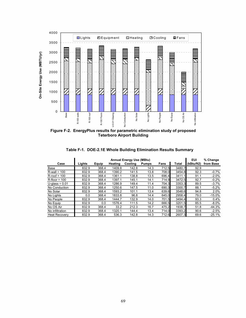
69
0
500
1000
1500
2000
2500
3000
3500
4000
Base
R-1
00 w
alls
R-1
00 ro
of
R-1
00 F
loor
s
U-0
.01
Gla
zing
No
Con
duct
ion
No
Sola
r
No
Ligh
ts
No
Peop
le
No
Equi
p
No
OS
Air
No
infil
tratio
n
On-
Site
Ene
rgy
Use
(MB
TU/y
r)Lights Equipm ent Heating Cooling Fans
Figure F-2. EnergyPlus results for parametric elimination study of proposed
Teterboro Airport Building
Table F-1. DOE-2.1E Whole Building Elimination Results Summary
EUI % ChangeCase Lights Equip Heating Cooling Pumps Fans Total (kBtu/ft2) from Base
Base 832.9 368.4 1409.8 142.8 14.3 712.5 3480.7 92.9R-wall = 100 832.9 368.4 1390.2 141.5 13.8 708.0 3454.8 92.3 -0.7%R-roof = 100 832.9 368.4 1361.1 138.8 13.5 696.4 3411.1 91.1 -2.0%R-floor = 100 832.9 368.4 1397.1 145.1 14.1 714.9 3472.5 92.7 -0.2%U-glass = 0.01 832.9 368.4 1286.9 149.4 11.4 704.3 3353.3 89.5 -3.7%No Conduction 832.9 368.4 1250.6 147.5 11.0 690.3 3300.7 88.1 -5.2%No Solar 832.9 368.4 1593.2 101.1 13.4 639.6 3548.6 94.8 2.0%No Lights 0.0 368.4 1833.8 96.8 14.4 645.0 2958.4 79.0 -15.0%No People 832.9 368.4 1444.7 132.9 14.0 701.5 3494.4 93.3 0.4%No Equip 832.9 0.0 1576.4 111.5 14.2 666.5 3201.5 85.5 -8.0%No OS Air 832.9 368.4 33.2 212.3 16.7 475.2 1938.7 51.8 -44.3%No infiltration 832.9 368.4 1320.1 144.4 13.4 714.0 3393.2 90.6 -2.5%Heat Recovery 832.9 368.4 536.3 142.8 14.3 712.6 2607.3 69.6 -25.1%
Annual Energy Use (MBtu)
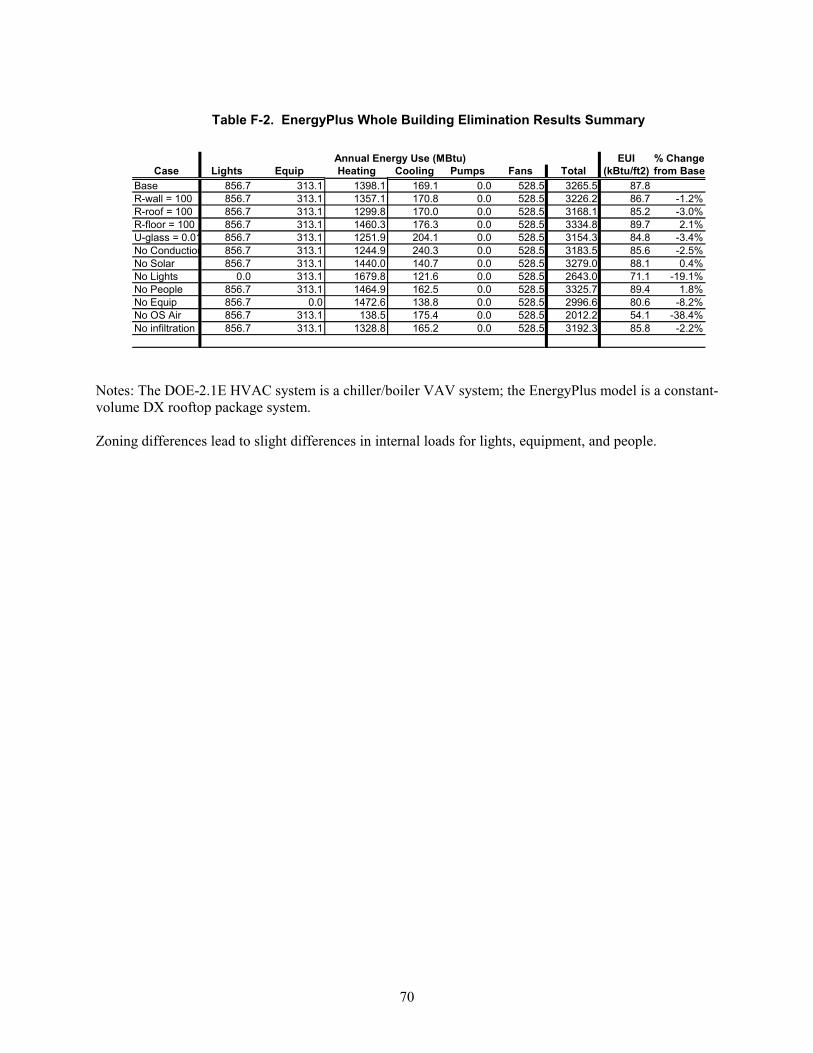
70
Table F-2. EnergyPlus Whole Building Elimination Results Summary
Notes: The DOE-2.1E HVAC system is a chiller/boiler VAV system; the EnergyPlus model is a constant-volume DX rooftop package system. Zoning differences lead to slight differences in internal loads for lights, equipment, and people.
EUI % ChangeCase Lights Equip Heating Cooling Pumps Fans Total (kBtu/ft2) from Base
Base 856.7 313.1 1398.1 169.1 0.0 528.5 3265.5 87.8R-wall = 100 856.7 313.1 1357.1 170.8 0.0 528.5 3226.2 86.7 -1.2%R-roof = 100 856.7 313.1 1299.8 170.0 0.0 528.5 3168.1 85.2 -3.0%R-floor = 100 856.7 313.1 1460.3 176.3 0.0 528.5 3334.8 89.7 2.1%U-glass = 0.01 856.7 313.1 1251.9 204.1 0.0 528.5 3154.3 84.8 -3.4%No Conduction 856.7 313.1 1244.9 240.3 0.0 528.5 3183.5 85.6 -2.5%No Solar 856.7 313.1 1440.0 140.7 0.0 528.5 3279.0 88.1 0.4%No Lights 0.0 313.1 1679.8 121.6 0.0 528.5 2643.0 71.1 -19.1%No People 856.7 313.1 1464.9 162.5 0.0 528.5 3325.7 89.4 1.8%No Equip 856.7 0.0 1472.6 138.8 0.0 528.5 2996.6 80.6 -8.2%No OS Air 856.7 313.1 138.5 175.4 0.0 528.5 2012.2 54.1 -38.4%No infiltration 856.7 313.1 1328.8 165.2 0.0 528.5 3192.3 85.8 -2.2%
Annual Energy Use (MBtu)

REPORT DOCUMENTATION PAGE
Form Approved OMB NO. 0704-0188
Public reporting burden for this collection of information is estimated to average 1 hour per response, including the time for reviewing instructions, searching existing data sources, gathering and maintaining the data needed, and completing and reviewing the collection of information. Send comments regarding this burden estimate or any other aspect of this collection of information, including suggestions for reducing this burden, to Washington Headquarters Services, Directorate for Information Operations and Reports, 1215 Jefferson Davis Highway, Suite 1204, Arlington, VA 22202-4302, and to the Office of Management and Budget, Paperwork Reduction Project (0704-0188), Washington, DC 20503. 1. AGENCY USE ONLY (Leave blank)
2. REPORT DATE
July 2003
3. REPORT TYPE AND DATES COVERED
Technical report
4. TITLE AND SUBTITLE Energy Design Analysis and Evaluation of a Proposed Air Rescue and Fire Fighting Administration Building for Teterboro Airport 6. AUTHOR(S)
B.Griffith; S. Pless; B. Talbert; M. Deru; P. Torcellini
5. FUNDING NUMBERS
BEC3.4005
7. PERFORMING ORGANIZATION NAME(S) AND ADDRESS(ES)
National Renewable Energy Laboratory 1617 Cole Blvd.
Golden, CO 80401-3393
8. PERFORMING ORGANIZATION
REPORT NUMBER NREL/TP-550-33294
9. SPONSORING/MONITORING AGENCY NAME(S) AND ADDRESS(ES)
10. SPONSORING/MONITORING
AGENCY REPORT NUMBER
11. SUPPLEMENTARY NOTES 12a. DISTRIBUTION/AVAILABILITY STATEMENT
National Technical Information Service U.S. Department of Commerce 5285 Port Royal Road
Springfield, VA 22161
12b. DISTRIBUTION CODE
1. 13. ABSTRACT (Maximum 200 words) A new/proposed building for the Teterboro Airport was selected as a case study for High
Performance Building Initiative research efforts. This report documents research-level energy analysis conducted on the
Teterboro Airport building during predesign and design phases of the project.
15. NUMBER OF PAGES
2. 14. SUBJECT TERMS High Performance Buildings; Teterboro Airport; New Jersey;
energy design analysis; building design analysis.
16. PRICE CODE
17. SECURITY CLASSIFICATION
OF REPORT Unclassified
18. SECURITY CLASSIFICATION
OF THIS PAGE Unclassified
19. SECURITY CLASSIFICATION
OF ABSTRACT Unclassified
20. LIMITATION OF ABSTRACT
UL
NSN 7540-01-280-5500 Standard Form 298 (Rev. 2-89) Prescribed by ANSI Std. Z39-18 298-102