Energy Efficient Connected Clusters forMobile Ad Hoc Networks

Sayan Mitra* and Jesse Rabek**�mitras,jesrab � @csail.mit.edu

MIT Computer Science and Artificial Intelligence Laboratory,32 Vassar Street,

Cambridge, MA 02139, USA

Abstract— A Mobile Ad Hoc Network (MANET) isa wireless infrastuctureless network with mobile nodes.Clustering is a common basis for building higher levelapplications for such networks. The merit of a clus-tered decomposition depends on the application thatis meant to use it. A power control based distributedclustering service is proposed that maintains clusterconnectivity under reasonable assumptions. The sizeand sparsity of the clustering can be controlled by twoparameters, namely, the minimal separation between theclusterheads, and the maximum angular gap betweenneighboring clusterheads. The optimal value of thelatter is derived; this minimizes the transmission powerof the clusterheads while guaranteeing connectivity ofthe cluster graph. Experimental studies presented showthat the algorithm rapidly stabilizes to a new clusteredorganization after the network topology changes due tonode joins and failures.

Index Terms— Ad hoc networks; Power control; Clus-tering algorithms; Cluster graph connectivity.

I. INTRODUCTION

In mobile ad hoc networks (MANETs) clustering isa common basis for building higher level applicationslike routing, tracking, and location management. Un-derlying every MANET application there are inherenttrade-offs between accuracy, energy consumption, ro-bustness, and memory requirements [22]. Accordingly,the merit of a clustered decomposition depends on theapplication which uses it. In a routing protocol, forexample, where each clusterhead maintains completeroute to all cluster members, smaller clusters implyless state maintained by the clusterhead and thereforeare preferable over larger clusters for scalability. Al-though small clusters result in a high latency betweennodes that are far apart in the network, this delay in

*The first author’s research is supported by AFRL contractnumber F33615-010C-1850.

**The second author was an M.Engg student at the Laboratoryfor Computer Science, MIT, at he time of this work.

message delivery is tolerated. Accordingly, the clus-tering schemes typically used for routing decomposethe network into 2-clusters. In contrast, for refer-ence broadcast based clock synchronization (RBS) [6]large, densely overlapping clusters are preferable. InRBS, each cluster behaves as a synchronized unit andtiming information is shared between nodes belongingto different clusters through common “gateway” nodesconstituting a time-routing path. Shorter the path, moreaccurate the synchronization between clusters. So, it isdesirable to have few large clusters spanning the entiregraph. In general, larger, heavily overlapping clustersimprove the robustness, accuracy, and latency of theapplication using the clusters, while adversely affect-ing the power consumption, memory requirements,and the longevity of the mobile nodes.

Irrespective of the size of the clusters, most applica-tions require the clusters to be connected. This can beachieved in an ad hoc fashion, by arbitrarily increasingthe broadcast radius of the clusterheads. This is unde-sirable for two reasons: first, it shortens the batterylife of the clusterheads because the power required totransmit a message over distance � increases as an����� degree polynomial of � , where ��� [20], andsecondly, it gives rise to extra interference.

In this paper, we propose a robust distributed clus-tering service which can produce the desired typeof clustering of a network for a wide range ofMANET applications. The size and the sparsity ofthe clustered decomposition are controlled by twoparameters, namely, � - the minimal separation be-tween clusterheads, and - the maximum allowedangular gap between neighboring clusterheads. Fur-ther, the algorithm minimizes the broadcast power ofthe clusterheads while guaranteeing the connectivityof the cluster graph. We prove that for any valueof � , the optimal value of is ������������ ���� (1.0107radians approx.), in following sense: this value of

minimizes the transmission power of the clusterheadswhile guaranteeing connectivity of the cluster graph,provided the given distribution of the mobile nodescan be connected when each node transmits withmaximum power.

The clustering service is implemented in two layers.The bottom layer selects the clusterheads based ona maximal independent set algorithm, such that eachclusterhead is at least � distance away from all otherclusterheads. The top layer decides the transmissionpower used by the clusterheads, based on certainlocally checkable condition. Specifically, each cluster-head increases its transmission power until it learnsabout another clusterhead (via some common node)in every -cone around itself. We discuss the differentclustered decompositions that can be obtained byrunning the algorithm with different � ���� �� settings.We also present experimental evidence supporting therobustness of the algorithm when subjected to changesin the underlying network topology owing to nodefailures and joins.

The rest of the paper is organized as follows: Thenext section cites and differentiates related work. InSection III the system model is described. In Sec-tion IV the details of the algorithms constituting theclustering service are presented. In Section V theoptimal value of the parameter , the angular gap, isderived and certain other optimizations to the basicclustering service are suggested. In Section VI thesimulation results evaluating the behavior of the algo-rithm with different parameter settings are presented,with respect to stability, robustness, and the generatedcluster topologies. Finally, Section VII concludes thepaper with a synopsis of the contributions and direc-tions for future research.

II. RELATED WORK

The notion of cluster organization has been used forad hoc networks ever since their appearance. In [2],[7] a distributed clustered architecture is introducedfor hierarchical routing. Gerla et. al. [9], [16] havepresented clustering algorithms for efficient resourceallocation, namely bandwidth and channel, in order tosupport multimedia traffic. Most clustering algorithmsproduce a 2-clustering of the network graph. Thegeneralization of this problem to k-clustering wasintroduced in [1], and used for routing in [13]. Itis known that k-clustering is NP-complete [5] forsimple undirected graphs. Fernandess and Malkhi [8]have given a polynomial time approximation algorithm

for k-clustering with ������ worst case ratio over theoptimal solution.

Most clustering algorithms including ours, work intwo phases. First, a subset of nodes in the network areselected to act as coordinators or the clusterheads. Thecriterion for selecting the clusterheads differ betweenalgorithms, the most common ones being based on thenode identifiers [2], [7], [9] and node degrees [17].In [3] a node mobility based criterion has been usedfor selecting the clusterheads to cope with dynamicchanges in the network topology. The second phase,which is typically initiated by the clusterheads, isconcerned with maintaining the extent of the clusters.A clusterhead may inform its member nodes abouttheir membership explicitly, by sending a message,or depending on the application, may just store themembership information in its own state.

Instead of sending messages expressly for impartingthe membership information to each member node,the clusterhead can periodically broadcast a beaconwith a particular transmission power to mark its ex-tent [14]. It has been shown in [10] that for a uniformdistribution of a large number of wireless nodes, acommon transmit power level is optimal with respectto the capacity of the network. In general, howeverthis is not true, and hence the need for clustering bypower control arises. In [12] two routing algorithmsare proposed which decide the transmit power for eachpacket, thereby implicitly creating transmission powerbased clusters. Our clustering service is closer to thealgorithm presented in [14], in that, we use powercontrol to explicitly maintain the extent of the clusters.

Varying the transmission power of nodes for effi-cient topology control in wireless networks was stud-ied in [19]. Li et al. [15], [21] describe a cone basedtopology control (CBTC) algorithm using directionalsensors which guarantees global connectedness. TheCBTC � �� algorithm increases the transmission powerof a node until there is a node within its transmissionradius in every cone of angle around it. It hasbeen shown in [21], [15] that for �� � ���� thepower settings obtained from CBTC � �� are sufficientfor maintaining connectivity. Hajiaghayi et. al. [11]presented a modified version of the CBTC protocolwith ��������� , to ensure k-connectivity of the network.Our algorithm for determining the transmission powerof each clusterhead is similar to CBTC but it maintainsconnectivity between clusters rather than individualvertices.

III. PRELIMINARIES

In this section we discuss our model and introducethe notations and definitions used throughout the restof this paper.

The mobile nodes are assumed to be distributed ina 2-dimensional plane and each node has an uniqueidentifier. Each node can broadcast messages at dif-ferent transmission power levels; the maximum power�

being the same for all nodes. The nodes do notpossess knowledge about their location in the plane,however they do have directional antennas, and acommon sense of direction. Having directional anten-nas is considered to be a reasonable assumption andhave been used elsewhere in the ad hoc networkingliterature (see, e.g., [15], [21], [4]). The common senseof direction can be achieved by means of a compass.

The mobile nodes can fail or migrate, and newnodes can join the network. When a node fails it losesits state. If a failed node recovers, it behaves as if itwere a new node and tries to join the network.

At a given instant of time the mobile ad hoc networkis represented as a directed graph ��� ��� ��� � , where� is the set of mobile nodes and � the set of edgesdetermined by the transmission power of the nodes.The transmission power � of node determines thetransmission radius, � ������ , and if is a cluster headthen � ��� � also defines the cluster around , which isthe set of nodes � ������� ��� ��� � ��� � � � �������� .

A clustering algorithm organizes a network of nodesinto a set of clusters ������ � � � � � �! #"$� . The clustercover � is characterized by its radius or size, andits sparsity. The radius of � is the radius of itslargest cluster in terms of physical distance, or thenumber of network hops. The size is the cardinalityof the largest cluster in � . The sparsity of � is ameasure of connectivity between the clusters. It is themaximum number of clusters to which any particularnode belongs. If � is a partition, that is, if all theclusters are disjoint, then sparsity is the maximumnumber of neighboring clusters of any cluster.

Definition 1. The cluster graph induced by aset of clusters � � �� � � � � � �! #"%� is the undi-rected graph & � �(' ��) � with ' � � and)*�+� �� #,�! # �%� #,.-/ #10�324� .

Definition 2. A path in a cluster graph &5� �(' ��) �is a sequence of clusters �� � � � � � �! 76 � , such that each #8:9�' and �� #8 �! #8<; � �/9�) for every �>=@? . Thecluster graph & is connected if there is a path betweenevery pair of cluster in ' .

IV. THE ALGORITHMS

The clustering service is implemented in two layers.The first layer, namely the Start Cluster algorithm(SC), maintains a set of cluster heads A , no twoof which are closer than a distance � , where � is aparameter of the algorithm. The second layer, namelythe Cluster Control (CC) algorithm, determines thebroadcast power of the clusterheads thus definingthe extent of each cluster. The broadcast power isdetermined by monitoring local membership and theoverlap with neighboring clusters. This ensures thatthe set of clusters cover the entire network and thatthe resulting cluster graph is connected.

A. Start Cluster Algorithm

The Start Cluster algorithm (SC) is a dynamicversion of the classical maximal independent set (MIS)algorithm [18]. The nodes selected to be in the set arethe clusterheads and all other nodes are the ordinarynodes.

Definition 3. The s-neighborhood BDC � �� of node isthe set of nodes within distance � from .

Definition 4. An s-independent set of a graph � withvertices � is a set of vertices A EF� , no two ofwhich are within a distance of G of each other. An s-independent set is maximal if no vertex can be addedto it without violating s-independence property.

In the classical MIS algorithm a node decides to be aclusterhead once and for all when it learns that all theneighboring nodes with higher identifier have decidednot to be clusterheads. And, a node decides to be anordinary node when it learns about a neighbor who hasdecided to be a clusterhead. Our reactive version of theMIS algorithm makes decisions for a finite interval oftime, and so it has to be executed repeatedly by everyparticipating node. This makes it possible for a nodeto take the necessary actions when there are significantchanges in its neighborhood. Once a node decidesto be a clusterhead, it remains a clusterhead for aninterval HJI , after which it continues to be a clusterheadonly if all the nodes with higher identifiers in its s-neighborhood are ordinary. A node decides to remainordinary for as long as it is aware of a clusterhead inits S-neighborhood, and renews its bid to become aclusterhead only when it stops hearing from the latter.

Every participating node executes the SC algorithmshown in Figure 1. The main subroutine decides if the

particular node is going to be a clusterhead or not, andthe messages thread handles the input messagequeue. Every decision message received by a nodeis stamped with an expiration time (TTL) measuredby the local clock ����� of the node. When node receives a

��������� � ��� � message from node � in itss-neighborhood, it adds � � , in an array � with a TTLH I time after the time of reception of the message.Node decides to become/remain a clusterhead attime ����� if it has received a decided(0) messagefrom every node in its s-neighborhood within the lastH I interval of time. The algorithm is said to havestabilized once all the nodes in the network � havedecided. Once the network stabilizes, and there are nofurther joins, failures, or migrations, the set of nodesA with � ��� constitute a maximal s-independentset of the network. In the worst case, stabilization maytake � � ���� 4? ��� ��� time.

message thread:

On receiving �������������������! #"%$'&)() if $'&+*-,.$'& ( then/ *1032 ; bcast �����+�������4�5�76� 8"�$7&)*4 with 9!*;:=< .

On receiving �����������������76� #"%$'&)() > * 0 > *@?BA ��$'&+(5"�CED�F *�GIH J %K

main:

initially/ J 0ML ; every H J time

If for every FONQP�R���S) TU$'&+VW,.$7& *X ��FY"�Z� [N > * "\Z],.CED4F * then/ * 0_^ ;

bcast �����+�����������\^` a"�$7& ( with 9!*;:=< .

Fig. 1. The Start Cluster algorithm. The decided(1) messageis sent when a node decides to become a clusterhead, whiledecided(0) is sent when a node decides otherwise.

B. Stability of SC

If the network topology changes owing to failure,migration, or joining of nodes, the algorithm regainsstability, in ��� � �� ? ��� ��� time, in the worst case. Webriefly discuss the performance of the algorithm ineach of these cases.

Joins: When a new node joins the network� , there are two possible scenarios that may arise.First, if is within the s-neighborhood of some othervertex � 9 A , then it receives the decided(1)message from � and immediately decides to be

an ordinary node. Otherwise, is outside the s-neighborhood of every node in A and it woulddecide to be a clusterhead within H I time. Therefore,in either case the algorithm regains stability within���8� � time.

Failures: When node 9 � fails, again thereare two possibilities. Let the network after thefailure be denoted �Bb . If �9 A , that is if is not aclusterhead then its failure does not affect the stabilityof the algorithm. Otherwise, 9 A then one ormore of the nodes in B1c�� �� would become eligible tobe a clusterhead. This change may propagate acrossthe network, and in the worst cast a new stableconfiguration would be achieved in � � ���� 4? ��� b ���time.

Migrations: When an ordinary node �9 Achanges its physical location it can be viewed as acombination of the above two cases. That is, it failsin its existing cluster and joins the cluster in its newlocation (or becomes a new clusterhead). On theother hand, if a clusterhead 9 A moves into B c �d� �for some other clusterhead � 9 A , then the situationis indistinguishable from the case where � migratesinto b�� cluster. We break the symmetry using someheuristics, e.g., the clusterhead with the larger clusterand the lower identifier remains a clusterhead andthe other node becomes ordinary. If 9�A then itsmovement would be indistinguishable from its failureto the nodes in B1c�� �� and this may trigger a completereorganization as discussed above.

Thus, under all possible scenarios the SC algorithmregains stability within ��� � �� 4? ��� ��� time. If the rateof failures, migrations, etc., in the network is nottoo large then the set A remains stable most of thetime. The Cluster control algorithm presented in thenext section relies on the stability of A to produce arobust clustered decomposition of the network.

C. Control Cluster Algorithm

The Control Cluster algorithm (CC) determines theminimum transmission power for each clusterheadssuch that the cluster graph is connected. The ideabehind CC is similar to the cone based topologycontrol algorithm (CBTC) of [15]. The algorithm isparameterized by a cone angle which can be tunedto change the sparsity of the cluster graph. The coneangle defines the e ��gf predicate which is the key

property that enables the clusterheads to guaranteeglobal connectivity.

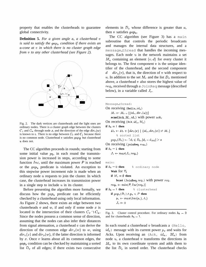
Definition 5. For a given angle , a clusterhead is said to satisfy the e ��gf condition if there exists an -cone at in which there is no cluster graph edgefrom to any other clusterhead (see Figure 2).

���� ����

��������

����

�������� � � ������� �

�

���� � ��� ���

�

Fig. 2. The dark vertices are clusterheads and the light ones areordinary nodes. There is a cluster graph edge between the clusters� * and

� V through node � , and the direction of the edge &�$79 * ��F1 is known to S . There is no edge between

� * and�!

because thereis no common node. Clusterhead S satisfies "$#&%(' ) but clusterhead* does not.

The CC algorithm proceeds in rounds; starting fromsome initial value �,+ , in each round the transmis-sion power is increased in steps, according to somefunction - �/. , until the maximum power

�is reached

or the e ��gf predicate is violated. An exception tothis stepwise power increment rule is made when anordinary node � requests to join the cluster. In whichcase, the clusterhead increases its transmission powerin a single step to include � in its cluster.

Before presenting the algorithm more formally, wediscuss how the e �� f predicate can be efficientlychecked by a clusterhead using only local information.As Figure 2 shows, there exists an edge between twoclusterheads and � , if and only if some node � islocated in the intersection of their clusters - 10 .Since the nodes possess a common sense of direction,assuming that the nodes can also infer their distancesfrom signal attenuation, a clusterhead can derive thedirection of the common edge ���32� � � � to � , using� �32 �(� � and � �32$4 � � � , if the latter direction is informedby � . Once learns about all its common edges, thee ��[f condition can be checked by maintaining a sortedlist 5 of all edges; if there exists two consecutive

elements in 5 whose difference is greater than ,then satisfies e ��gf .

The CC algorithm (see Figure 3) has a mainsubroutine that controls the periodic broadcastsand manages the internal data structures, and amessage thread that handles the incoming mes-sages. Each node � in the network maintains a set6 , containing an element � ��� � for every cluster itbelongs to. The first component is the unique iden-tifier of the clusterhead, and the second component� � ���32�, � �� , that is, the direction of with respect to� . In addition to the set

6 and the list 5 mentionedabove, a clusterhead also stores the highest value of287$9 , received through a JoinReq message (describedbelow), in a variable called :4 .

Message thread:

On receiving �<;��>=?=?@ "�$7& ( A *;0 A * ? A ��$'& ( "%&�$79!*�� * � %KBDCFEHG �JI)�LK�" A * "%$7& * with power #$MDN *On receiving �JI+�LKE"�$7&)(5" A () if/ Jg:O^ thenO * 0 O * G A &�$79!*+�J�E QPg��$7&$R "�&�$79 ( �J�E � gN A ( K

% sorted list

"$#&%TS)� O * 0 X &$U�N O * "VP &$UXW &$UZY\[VP$]^#On receiving �`_a@��Vb?c+�edE"\9afLg!(+ if/ Jg:O^ thenh * 0jik#$��� h * "�9afLg`()

main:

if/ Jg: 2 then % ordinary node

Wait for H JifA * :ml then

bcast �ona@��Vbac+�ad5"�9efLg * with power 9efLg *9afLg * 0piQ$7C��rq]"3s�C8M���9efVg * �

if/ J :O^ then % clusterhead

if "$#V%tS+� O * Tu% *wv q then

% * 0pix#y���Js�CXM4�z% * a" h * h * 032

Fig. 3. Cluster control procedure. For ordinary nodes/ J : 2

and for clusterheads/ J :O^ .

In each round a clusterhead broadcasts a (Hello,��� ) message with its current power � and waits forAcks. Upon receiving an (Ack, ��� , , 6 , ) fromnode � , a clusterhead transforms the directions in6 , to its own coordinate system and adds them tothe list 5 in sorted order. The clusterhead checks

the e ��[f condition by computing differences betweenconsecutive members of 5: . If the e ��gf condition issatisfied and the transmission power is less than themaximum power

�, then the tentative transmission

power for the next round is increased according tosome function - �/. . The actual power used for broad-cast is the maximum of this tentative power and : .

An ordinary node upon receiving a (Hello,��� , ) message adds �(��� , ��� �32 �d� ��� to its membershipset

6 and transmits an (Ack, ���4 � 6 ) messagewith power . �� . The power . �� is locallydetermined by such that it is sufficient to eitherreach some intermediate node that can forward themessage to � , or it reaches � directly. If it times outbefore receiving a Hello message then it sends a(JoinReq, 2 7y9 ) message with power 287y9� to thenearest known clusterhead. If there is a clusterhead bwithin � distance from , then sends the JoinReqto b , otherwise performs a discovery process bybroadcasting JoinReq with increasing power untilit receives a Hello message.

For small values of , the e ��gf predicate is easierto satisfy, and the broadcast power of a clusterheadhas to be high in order to discover nodes whichare farther away and learn about other clusterheads.On the other hand, with large values of the e �� fcondition might be violated with a small broadcastradius, but this may result in disconnected clusters.Therefore, we have to find the maximum value of which ensures connectivity of the cluster graph. Inthe next section we derive this value of for a staticnetwork.

V. OPTIMAL CONE ANGLE FOR POWER

EFFICIENCY AND CONNECTIVITY

Given a network � � ��� ��� � and a set A E5� ofclusterheads, let & �� and & f� be the induced clustergraphs corresponding to every � 9 A transmittingwith maximum power

�and the power assigned by

CC( ) algorithm, respectively. We shall prove that for �� 4" f 4 � �� ��� ��� � ���� , the cluster graph & f� isguaranteed to be connected if & �� is connected. Thevalue 4" f 4 corresponds to the angle at the center ofa circle with radius

�subtended by the intercepts of

an arc of radius � drawn with the same center withanother circle of radius

�touching the first circle (see

Figure 4). For proving the above statement we makeuse of the following geometric Lemma:

�� �

������

Fig. 4. Geometric interpretation of the maximal cone angle # : �������� [�� [��� : the angle subtended at the center of a circle fromthe intercepts of an adjacent circle with the same radius and aconcentric circle with double the radius.

Lemma 1. Consider a point � on the line segment � such that � ���D� � � and � � � � � , and any point� on the line ��� making ����� � ����� ��� � ���� . If � =� � � � =�� � � , then ?>� � ��� � � � � � � � � � � .

Proof. See the appendix.

Theorem 1. If � ������ ��� � ���� then & f� preservesconnectivity of & �� ; for ����39 A , f, and f areconnected iff �, and � are connected.

Proof. Given the same set of clusterheads A , theinduced cluster graph & f� is a subgraph of the clustergraph & �� , therefore it is clear that if f, �! f areconnected then �, �!

� must also be connected. We

prove the converse as follows.Suppose cluster graph � �� is connected while � f �

is not. So, there exists at least one pair of clusters, suchthat there is no path between them in & f� . We selectone such pair f, �! f , for which the distance betweentheir clusterheads, � � ��� �d� ���� is the smallest. Since & ��is connected we know that ��� ��� �d� ���� � � and thatthere exists a vertex � 9 �, - � . Since � �9 f, -. f ,it follows that the radius of the clusters f, and fcannot both be equal to

�. At least one of the radii is

less than�

, let us assume without loss of generalitythat 2 , = � , therefore 2 � � . Then, � must haveterminated the % �� �� with e ��]f � 5 , �/� ��!�" #%$ , thatis, there exists an edge between � and some otherclusterhead within the cone bisected by � (as shownin Figure 5). Let � be such a cluster head that makesthe angle & minimum. Therefore, & � ����������� ���� , and� � � 2�,(' 2 0 � 2�,)' � = � . From Lemma 1 weknow that either � 9 �0 or /9 �0 . In other words, �0 and � are connected in & �� .

Since � = � � = � , and & = � � , it follows

that � = � . By our assumption f0 and fare not connected. So we have a pair of clusters �, �!

�0 which are connected in & �� but not in & f� ,

with � � ��� �d��� � �+= � � ��� �d� ���� . This contradicts ourassumption that � �� were the closest such pair ofdisconnected clusterheads.

To show that the above value � ������ ��� � ���� is infact the maximum possible value ensuring connectiv-ity, we construct a simple counterexample. Considerthe scenario where ' � is used as the cone angle forthe e �� condition (Figure 5). The clusters �, and �are connected through vertex � . Owing to the presenceof the node � within

�����distance of � , there is an

edge between f!; ���, and f!; ���0 in the upper half & ' � -cone. Similarly, there is an edge between f!; ���, and f!; ���� . Clusterhead � , therefore, violates the e ��@f!; ���condition and terminates the cluster control algorithmwith a � ���� � � ��� . As a result � �93 f ; ���, , and f!; ��� is not connected to the rest of & f ; ��� .

x

�

�

�

�

������������

Fig. 5. Clusterhead uses a "$#&%tSVY���� criterion which makes itsradius � W! , disconnecting cluster

� * .

A. Optimizations

It is possible that the power assigned by the CCalgorithm described above is too high for a cluster-head after new nodes join in its neighborhood. Inthis section we present some optimizations to thebasic CC algorithm to improve its efficiency undersuch dynamic conditions. Essentially, a clusterhead should shrink its broadcast radius from a high value� b to a lower value � when the member nodes at adistance farther than � ��� � do not contribute to 5 .The Shrink back procedure, shown in Figure 6 isinvoked by the cluster control algorithm to reduce thetransmission radius.

Shrink back(c):" *;0 A * P * N � *@T � A ( : A $7&+*�K4 %K"$#* 0 � *&% " *& * 0pix#$��(('*),+4&�$.-#Z8��S5" * & # * 0pix#$� (('*)0/+ &�$.-#Z8��S5" * O #* 0 A &�$79!*)�J�� P ��$7&$R "�&�$79 ( �J�E � [N A ( T &�$.-#Z8� * "\S) &1.& # * W M!Kif �<"$#V% S � O *4 0243\"$#V% S � O #* T ��& # * W M1,.&+*�

then &��z% * �0M& # * W M

Fig. 6. Shrink back optimization. M is a parameter of the procedurewhich determines how aggressively the broadcast radius is cutdown.

Clusterhead keeps record of the distance to thefarthest member node which actually contributes to-wards satisfying the e �� predicate. The sets 5 and5 b are complementary subsets of : 5. is the setof nodes which do not belong to any other cluster; � and � b are the corresponding distances to the farthestnode. Clearly, can not shrink the cluster radius below�� , because that would make some of the nodes in5 cluster-less. The set 5 b is the set of directionsin which has edges via nodes which are closer than� b � . . The the broadcast radius is reduced to a � b � . ,if this does not create new gaps, and if the new radiusdoes not exclude any of the nodes in 5 .

VI. SIMULATION

In this section we study the performance of the clus-tering service through simulation based experiments.We observe the cluster graph topologies generated bysetting different values of the parameters � and andthe robustness of the algorithm under dynamic changesin the network topology due to node joins and failures.

Our discrete event simulator, implemented in C++,emulates individual mobile nodes with asynchronouscommunication. For the results presented in this sec-tion we have used a set of 100 nodes placed in a2-dimensional plane of 300x300 square units. Thenodes are distributed randomly in the plane such thateach node lies within the maximum broadcast distanceof at least one other node; this guarantees that theunderlying network is connected when all the nodesbroadcast with maximum transmission power.

A. Cluster Graph Topology

One of the main advantages of our clustering serviceis that, one can control the type of clustered decompo-sition of the network by appropriately setting the � and

(a) � =20 =1.01 (b) � =30 =1.01 (c) � =30 =1.57

(d) � =40 =0.8 (e) � =60 =1.01 (f) � =50 =1.57Fig. 7. Generated Network Topologies for Different Values of - and # . Dark dots are the ordinary nodes, and light dots with outerconcentric circle are the clusterheads. A line between nodes * and S indicates the presence of an edge between clusters

� ( and� * in

the cluster graph.

. Figure 7 shows the qualitatively different clusteringsthat were generated by the service on the same distri-bution of mobile nodes. In Figure 7(a), the minimaldistance between clusterheads �/� � is small, as aresult a large fraction of the nodes in the network areclusterheads. The cone angle is set to � ��� � radians,which is close to the maximal cone angle ( � ��� � ���radians) prescribed by Theorem 1, and therefore thecluster graph is sparsely connected. In comparison, thecluster graph of Figure 7(b) with �.� � � has fewerclusterheads but they are more densely connected.Increasing the cone angle keeping � fixed at � � weobserve (Figure 7(c)) that the sparsity of the clustergraph increases. Increasing � to � � and reducing thecone angle to � ��� results in a further decrease inthe number of clusterheads and gives the densely con-nected cluster graph of Figure 7(d). With larger values

of , the e ��gf predicate in the CC algorithm is violatedwith a lower power level for clusterheads which aresurrounded by other clusterheads, and therefore theresulting cluster graph is sparser with smaller clusters.Comparing Figures 7(e) and 7(f) to Figures 7(b)and 7(c) respectively, we observe that for the samevalue of , increasing � results reduction in the numberof clusterheads and an increase in the sparsity of thecluster graphs.

In general, with larger values of � the connectivityof the cluster graph, the size of the clusters, andthe power consumed increases, while larger valuesof decreases connectivity and size of the clusters.Therefore, based on the requirements of a particularapplication the values of � and can be so chosen asto produce desirable clustered decomposition.

B. Average Cluster Degree

Unlike sparsity (the maximum cluster degree), theaverage cluster degree measures how well the clustergraph is connected, on an average. Average cluster de-gree is an important robustness metric because it tellsus the number of neighboring clusterheads that can failbefore an average clusterhead gets disconnected fromthe rest of the cluster graph. The degree of cluster is obtained simply by counting the number of elementsin the set 5 . We take the average over all clusters andobserve this value over time as the service stabilizes(Figure 8).

Our first observation is that, with � � � � the stablevalue of the average cluster degree is higher than thatwith � � � , irrespective of the value of . Secondly,for each value of � , the average cluster degree is higherfor a smaller value of . Both these observations are inaccordance with our expectations as explained in theprevious section. It is to be noted that, for large valuesof � , a smaller fraction of clusterheads are locatedat the edge of the grid. Since, these edge clustershave fewer neighboring clusters, and therefore a lowercluster degree, the average degree of the cluster graphis lower than what would be expected otherwise.

Fig. 8. Average degree of the clusterheads.

C. Stability after Failures and Joins

In this section we study the robustness of the clus-tering service under dynamic changes in the underly-ing network topology. The network topology changeswhen mobile nodes move, fail, or new nodes jointhe network, and we are interested to examine thestabilization time, that is, how quickly the remaining

nodes of the network reach a agreeable state wherethey are organized into a cluster graph. In the simulatorwe measure stabilization time as follows: First we letthe CC algorithm stabilize on the initial network of100 randomly distributed mobile nodes; then, a certainnumber randomly chosen existing nodes are failed ornew nodes are added in random locations, and weobserve the number of rounds required for the networkto re-stabilize. The number of execution rounds forre-stabilization give us an indirect measure of timerequired by the algorithm to reorganize the network.

0 2 4 6 8 10 1230

40

50

60

70

80

90

Rounds

Num

ber

of s

tabl

e no

des

Stabilization after failure of 10 nodes from a network of 100

s=40 a=3s=40 a=1s=20 a=3

0 2 4 6 8 10 1220

30

40

50

60

70

80

Rounds

Num

ber

of s

tabl

e no

des

Stabilization after failure of 20 nodes from a network of 100 nodes

s=40 a=3s=40 a=1s=20 a=3

Fig. 9. Stabilization after node failures. Large and heavilyoverlapping cluster stabilize faster than small and sparse clusters.

The plots in Figure 9 show the changing numberof stable nodes in the network after the set of nodeshave failed. Initially the number of stable nodes de-creases as the effect of failure propagates through thenetwork, but this effect stops and eventually the newcluster structure emerges leading to stability of all

the remaining nodes in the network. As expected, weobserve larger clusters with greater overlaps ( � � � � )regain stability more quickly than smaller clusters( � � � ). A smaller results in larger clusters andmore overlaps, but also takes longer time for thecluster control algorithm to terminate, so the effectsof on the the network stabilization time is complexand dependent on the number of failed nodes.

We performed a similar set of simulations withnew nodes joining the stable network of 100 mobilenodes (Figure 10). There are two opposing effects thatdetermine the total time to stabilize the network in thiscase: first, with larger clusters ( � � � � ) larger fractionof the new nodes turn out to be ordinary nodes andtherefore are stable right when they join the network.This makes the initial number of stable nodes largefor large values of � . Secondly, small and denselyconnected clusters ( ��� � , +� � ��� � ) react moresharply to new nodes than large and sparse ( � � � � , � � ) clusters.

0 2 4 6 8 10 12 14 16 18 20101

102

103

104

105

106

107

108

109

110

111

Rounds

Num

ber

of S

tabl

e N

odes

Stabilization After Nodes Join

s=20 a=1.01s=40 a=0.5s=40 a=3s=40 a=1.01

Fig. 10. Stabilization of algorithm after new nodes join thenetwork. With larger values of - , fewer nodes are unstable initially,but the response of the clusterheads in absorbing the new nodesis also slower.

D. Network Longevity

Our last set of simulation results deal with thelongevity of the mobile network with the nodes ex-ecuting the clustering algorithm. We assume that eachnode is equipped with identical battery packs. Thebattery power consumed to transmit over a distance� is an ����� degree function of � , where � � � � .For this simulation we assume that no new nodes jointhe network, the only failures are due to battery power

outage, and that the nodes are static. Typically, theordinary nodes broadcast infrequently and over shortdistances and the clusterheads broadcast frequentlyover longer distances. Therefore, clusterheads wouldtypically run out of battery and die sooner than theordinary nodes. Once a clusterhead dies, an ordinarynode takes up the job of being the clusterhead andthe cycle continues until the very last node runs outof power. The early expiration of the clusterheads canbe mitigated by systematically rotating the broadcastresponsibility of the clusterhead within the cluster,however we have not implemented this modificationin our algorithm in presenting the following results.

Figure 11 shows the number of surviving nodesas the execution of the algorithm progresses overtime. With large, dense clusters ( �/� � ���� ��� ��� � ),there is a distinct ’knee’ in the curve beyond whichthe number of surviving nodes diminish sharply. Incontrast, sparser clusters ( �>� � ���� � � ) result in agradually degrading network. Further, when the ( � �� ���� 1� � ��� � ) curve starts to drop at the ’knee’ point,the number of surviving nodes on ( � � � ���� >� � ) isalready down to 45. Therefore, form the point of viewof longevity, the preferred type of clustering would bedetermined by the type of degradation desired of thenetwork.

0 10 20 30 40 50 60 700

10

20

30

40

50

60

70

80

90

100

110Node Longevity

Time Elapsed

Per

cent

age

of li

ve n

odes

s=40 a=3s=40 a=1.01s=20 a=3

Fig. 11. Lifespan of network executing the clustering algorithm.There is a distinct knee in the curve for large dense clusters( - :� 2+"3# : ^�� 2+^ ), whereas sparse clusters ( - : 2)" � 2)"3# :�� ) resultin a graceful degradation of the network.

VII. CONCLUSIONS

The merits of a clustered decomposition for a givennetwork graph depends on the MANET application

which uses the clustering. For most applications,however, it is desirable to have a connected clustergraph. In this paper we have proposed an adaptiveclustering service that can be tuned to suit particularMANET applications. The cluster control algorithmminimizes the transmission power of the clusterheadswhile guaranteeing that the produced clusters areconnected whenever it is physically possible.

The clustering service does not rely on globallocation information. Two parameters � - the inter-cluster distance and - the maximum allowed angulargap between neighboring clusterheads, are used tocontrol the size and sparsity of the clusters producedby the service, and thereby achieve the desired trade-offs among latency, energy efficiency, and robustness.We have shown that �� ��� ��� � ���� (approx. 1.0107 rads)is the optimal value of which minimizes the trans-mission power of the clusterheads while guarantee-ing connectivity of the cluster graph, provided thatthe underlying network is connected when all nodesbroadcast with maximum power. We have presentedexperimental results showing the qualitatively differ-ent type of clustered organizations that can be ob-tained from the algorithm. Our simulation experimentsdemonstrate that the algorithm rapidly recovers frominstability caused by node failures and joins.

The empirical evidence presented here suggests thatthe algorithm has nice self stabilization properties; inthe future we plan to rigorously analyze its behaviorunder dynamic topology changes and also extend theresults to three dimensional distribution of mobilenodes. Our long term goal is to focus on particularMANET applications (e.g., tracking, routing), anduse this clustering algorithm in conjunction with thechosen application to examine the performance of theapplication as a function of the cluster metrics.

VIII. ACKNOWLEDGMENTS

The authors would like to thank to Ben Leong andHari Balakrishnan for their comments and suggestionson this work.

REFERENCES

[1] R. Prakash A. Amis, T. Vuong, and D. Huynh. Max-min d-cluster formation in wireless ad hoc networks. InProceedings of IEEE INFOCOM, pages 32–41, March 1999.

[2] D. J. Baker and A. Ephremides. The architectural organiza-tion of a mobile radio network via a distributed algorithm.IEEE Transactions on Communications, COM-29(11):1694–1701, Nov 1981.

[3] S. Basagni. Distributed clustering for ad hoc networks.In Proceedings of the IEEE International Symposium onParallel Architectures, Algorithms, and Networks (I-SPAN),pages 310–315., Perth, Western Australia, June 1999.

[4] R. Choudhury and N. Vaidya. On ad hoc routing using di-rectional antennas. In Illinois Computer Systems Symposium(iCSS), 2002.

[5] J. S. Deogun, D. Kratsch, and G. Steiner. An approximationalgorithm for clustering graphs with dominating diametralpath. Information Processing Letters, 61(3):121–127, Febru-ary 1997.

[6] Jeremy Elson, Lewis Girod, and Deborah Estrin. Fine-grained network time synchronization using reference broad-casts. SIGOPS Oper. Syst. Rev., 36(SI):147–163, 2002.

[7] A. Ephremides, J. E. Wieselthier, , and D. J. Baker. A designconcept for reliable mobile radio networks with frequencyhopping signaling. In IEEE, volume 75, pages 56–73, Jan1987.

[8] Yaacov Fernandess and Dahlia Malkhi. K-clustering inwireless ad hoc networks. In Proceedings of the second ACMinternational workshop on Principles of mobile computing,pages 31–37, Toulouse, France, 2002. ACM Press.

[9] M. Gerla and J. Tsai. Multicluster, mobile, multimediaradio network. ACM/Baltzer Journal of Wireless Networks,1(3):255–265, 1995.

[10] P. Gupta and P. Kumar. Capacity of wireless networks. InIEEE Transactions on Information Tehory, volume IT-46,pages 388–404, 2000.

[11] M. T. Hajiaghayi, M. Bahramgiri, and V. S. Mirrokni.Fault-tolerant and 3-dimensional distributed topology controlalgorithms in wireless multi-hop networks. In Proceedings ofthe 11th IEEE International Conference on Computer Com-munications and Networks (IC3N), pages 392–398, Miami,Floria., October 2002.

[12] Vikas Kawadia and P. R. Kumar. Clustering by power controlin ad hoc networks. In Proceedings of IEEE MILCOM,Atlantic City, NJ, October 1999.

[13] P. Krishna, N. Vaidya, M. Chatterjee, and D. Pradhan. Acluster-based approach for routing in dynamic networks. InACM SIGCOMM Computer Communication Review, pages49–65, April 1997.

[14] Taek Jin Kwon and Mario Gerla. Clustering with powercontol. In Proceedings of IEEE MILCOM, Atlantic City,NJ, October 1999.

[15] Li Li, Joseph Y. Halpern, Paramvir Bahl, Yi-Min Wang, andRoger Wattenhofer. Analysis of a cone-based distributedtopology control algorithm for wireless multi-hop networks.In Proceedings of the twentieth annual ACM symposium onPrinciples of distributed computing, pages 264–273. ACMPress, 2001.

[16] Chunhung Richard Lin and Mario Gerla. Adaptive clusteringfor mobile wireless networks. IEEE Journal of SelectedAreas in Communications, 15(7):1265–1275, 1997.

[17] A. K. Parekh. Selecting routers in ad hoc wireless networks.In ITS, 1994.

[18] David Peleg. Distributed computing: a locality-sensitiveapproach. Society for Industrial and Applied Mathematics,2000.

[19] Ram Ramanathan and Regina Hain. Topology control ofmultihop wireless networks using transmit power adjustment.In INFOCOM (2), pages 404–413, 2000.

[20] Theodore Rappaport. Wireless Communications: Principlesand Practice. Prentice Hall PTR, 2001.

[21] Roger Wattenhofer, Li Li, Paramvir Bahl, and Yi-Min Wang.Distributed topology control for wireless multihop ad-hocnetworks. In INFOCOM, pages 1388–1397, 2001.

[22] Bhaskar Krishnamachari Yasser. The energy-robustnesstradeoff for routing in wireless sensor networks.url:citeseer.nj.nec.com/552652.html.

APPENDIX

Proof of Lemma 1.

Proof. Draw circles � and 5 with radii�

and centers� and , respectively. Let the points of intersection of��� with � and 5 be . , � , and ��b respectively. Weconsider three cases based on the position of � in ���(see Figure 12).

v

(a) (b)

��

�

�

���

�

� �

�

��

�

�

�

�

� �� �

�

��

�

Fig. 12. Nodes are present at * , S , � , and F which is any pointon *�� , with P * SXP[, P * F P .(a) Cases 1 and 2: node F is locatedeither inside circle � or

". (b) Case 3: node F is between M and�

but outside both � and"

.

Case 1: � is located to between � and � . Let � bbe the closest possible location of � from � . Since��� � & = � ���� and � � � b � = � � � it follows that �����and ����� ��� � ���� . Using ��� �"!# ,� # �$��� �&%# 0&/ # , we get � � b ���� � � � � � . Therefore, for any location of � in � � b ,� � ��� � .

Case 2: � is located between . and � . From � ���D� ��, � � �*� � , and & = � � , it follows that � � . � � � .

Therefore, for any location of � in � , � �k. ��� � .Case 3: � is located in between . and � and outside

of both � and 5 (Figure 12(b)). First we show that� �'� ��� � . Let ��� be a tangent to 5 on the same side of� as � � . Since � � J� � � , it follows that � ����� � � .

Therefore � �'� � � � . From case 2 it is known that� � . � � � , it follows that for any position of � between and � , � � � ��� � .