Energy Efficient Node Deployment for Target Coverage in Wireless Sensor Network

Prepared By : Gaurang Rathod ME EC Gujarat Technological University Gujarat India

29 January 2015 rathodgaurang@hotmail.com

Outline

Motivation Introduction Network Lifetime for Target Coverage ABC Algorithm Simulation Work References

Motivation Wireless sensor network is energy constrain

network

Energy consumption of Node[1]

1. Data transmission2. Signal processing 3. Hardware operation

Target Coverage Coverage can be classified as area coverage

and target(point) coverage[6]

(a) Area coverage and (b) Point coverage

Continue… Target Coverage can be categorized

1. Simple coverage

2. k-coverage

3. Q-coverage: Target T= {T1,T2,..,Tn} should be monitored by Q= {q1, q2,…, qn} number of nodes

Network Lifetime Network is live till all targets being sensed

by nodes otherwise network considered as dead.

Network life is defined by target sensed time duration by nodes.

Deploy nodes such a way that target sensed by maximum number of nodes, so network live long.

Node Deployment Algorithm Input: no. of nodes and no. of target

Output: optimum location of node such that maximum network life achieve with required target coverage level

Procedure1. Select random location for the given no. of target.2. Deploy nodes randomly such that each target must be

covered by minimum one node.3. Compute life time of network.4. Recomputed node position using ABC algorithm such

that network life maximum.

Network Lifetime Calculation Let sensor nodes : {s1, s2, s3,…,sm}

randomly deployed to cover the region R with n targets : {T1,T2,..,Tn}

Each node has initial energy E0 and a sensing radius sr

A sensor node is said to cover target if distance between node and target is less than radius sr

Coverage Matrix is defined as

1

0i j

i j

if S monitorsTM

otherwise

Continue…

where ei is energy consumption rate of i-node

For k-coverage, qj=k, j=1,2,…,n

0( ) , 1Lifeof node ii

Eb i m

e

1

*

minNetwork lifetime

m

i j ii

j

M b

j q

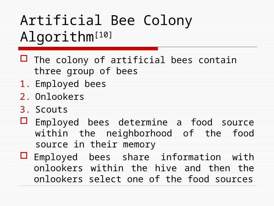
Artificial Bee Colony Algorithm[10]

The colony of artificial bees contain three group of bees

1. Employed bees2. Onlookers3. Scouts Employed bees determine a food source within

the neighborhood of the food source in their memory

Employed bees share information with onlookers within the hive and then the onlookers select one of the food sources

Continue… Onlookers select a food source within the

neighborhood of the food sources chosen by themselves

An employed bee of which the source has been abandoned becomes a scout and starts to search a new food source randomly

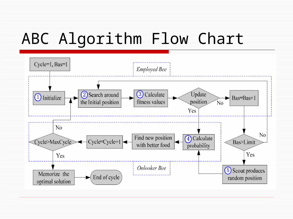
ABC Algorithm Flow Chart

Continue..

Image source: http://commons.wikimedia.org/wiki/File:Maxima_and_Minima.svg

Continue… New search position

i=bee indexj=random selected dimension i.e. either x-yam or y-yam random selectedk=random selected bee (k never equal to i)

, , , ,( )i j i j i j k jv x x x

Simulation

A. Target Coverage

B. Importance of Deployment and Scheduling

Experiment Work A

1. For fix number of targets and varying number of nodes

2. For different-different number of targets and nodes

3. For changing size of network

4. By varying sensing range of node

Simulation Parameters

Parameter Value

Network area 400m x 400m

500m x 500m

Node sensing range 75m

80m

Initial energy 100 J

Energy consumption rate 1 J/S

No. of target 20 to 40

No. of nodes 100 to 250

Network Lifetime for 20 Targets

Network size: 500m x 500m, sensing range: 75m

Network Lifetime for 25 Targets

Network size: 500m x 500m, sensing range: 75m

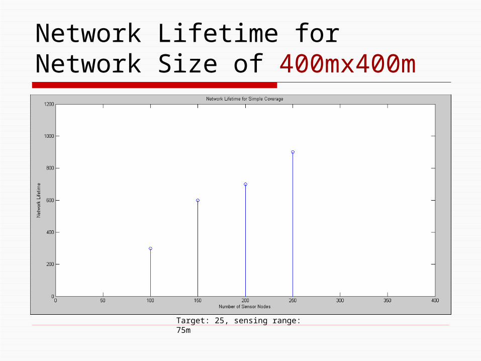
Network Lifetime for Network Size of 400mx400m

Target: 25, sensing range: 75m

Network Lifetime for Network Size of 500mx500m

Target: 25, sensing range: 75m

Network Lifetime for 75m Sensing Range of Node

Target: 25, Network size: 500m x 500m

Network Lifetime for 80m Sensing Range of Node

Target: 25, Network size: 500m x 500m

Network Lifetime for Random Deployment

Network size: 500m x 500m, sensing range: 75m

Deployment using ABC algorithm

Network size: 500m x 500m, sensing range: 75m

Network Lifetime for K-Coverage (Random Deployment)

Network size: 500m x 500m, sensing range: 75m

Network Lifetime for K-Coverage (Deployment using ABC Algorithm)

Network size: 500m x 500m, sensing range: 75m

Experiment Work B

Simulation Cases :

1. Node deployment with same communication interval

2. Node deployment with distinct random communication interval

3. Node deployment with distinct communication interval base on communication cost

Simulation ParametersParameter Value

Channel Type Wireless 802.15

Propagation Type Two Ray Ground

MAC protocol MAC – 802.15

Queue Type Drop tail

Antenna Omni Antenna

Number of nodes 25

Queue Length 50

Routing protocol AODV

Network area 500 m x 500 m

Packet size 200 bytes

Initial Energy 2 joules

29

Case 1 : Node Deployment with Same Communication Interval

Residual Energy of All nodes vs Time

Case 2: Node Deployment with Distinct Random Communication Interval

Energy is inversely proportional to square of the distance

Node far from the base station consume more energy compared to near one

By allocating different communication interval to each node helpful to make network energy consumption rate balance compared to case 1

Residual Energy of All nodes vs Time

Case 3: Node Deployment with Distinct Communication Interval Based on Communication Cost

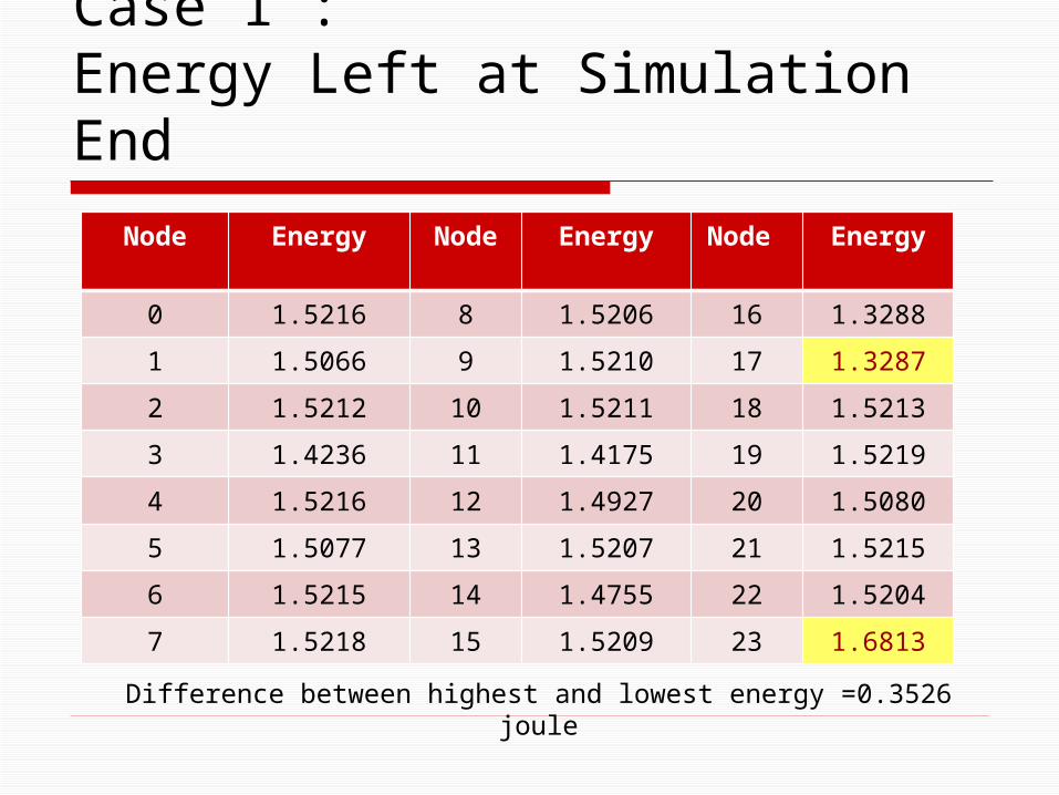
Case 1 :Energy Left at Simulation End

Node Energy Node Energy Node Energy

0 1.5216 8 1.5206 16 1.3288

1 1.5066 9 1.5210 17 1.3287

2 1.5212 10 1.5211 18 1.5213

3 1.4236 11 1.4175 19 1.5219

4 1.5216 12 1.4927 20 1.5080

5 1.5077 13 1.5207 21 1.5215

6 1.5215 14 1.4755 22 1.5204

7 1.5218 15 1.5209 23 1.6813

Difference between highest and lowest energy =0.3526 joule

Case 2 : Energy Left at Simulation End

Node Energy Node Energy Node Energy

0 1.6736 8 1.6847 16 1.6849

1 1.6383 9 1.6450 17 1.6714

2 1.6823 10 1.6851 18 1.7172

3 1.6827 11 1.6812 19 1.6004

4 1.6968 12 1.6838 20 1.6808

5 1.6346 13 1.6857 21 1.6819

6 1.6686 14 1.6608 22 1.6600

7 1.6786 15 1.6441 23 1.6813

Difference between highest and lowest energy =0.1168 joule

Case 3 :Energy Left at Simulation End

Node Energy Node Energy Node Energy

0 1.8562 8 1.8585 16 1.8534

1 1.8582 9 1.8563 17 1.8561

2 1.8592 10 1.8588 18 1.8572

3 1.8586 11 1.8576 19 1.8586

4 1.8566 12 1.8592 20 1.8527

5 1.8455 13 1.8589 21 1.8580

6 1.8592 14 1.8424 22 1.8554

7 1.8480 15 1.8597 23 1.8505

Difference between highest and lowest energy =0.0173 joule

Conclusion Sensing range of node, size of network, number of

target, number of nodes and scheduling have significant effect on life of network which we have done analyses in the simulation by increasing no. of target and sensing area network life decrease but by increasing node’s sensing radius life increases with effective coverage level.

By using artificial bee colony algorithm for node deployment, we achieve the required target coverage level and maximize the network lifetime compared to random deployment. Node deployment by using ABC algorithm work good for simple as well as k-coverage application.

References1. I. Akyildiz, W. Su, Y. Sankarasubramaniam, and E. Cayirci, “A survey on

sensor networks”, IEEE Commun. Mag., vol. 40, no. 8, pp. 102–114, Aug. 2002.

2. Karl, Holger and Andreas Willig, “Protocols and Architectures for Wireless Sensor Networks”, John Wiley & Son Ltd, 2005.

3. I. Akyildiz and M. Vuran, “Wireless Sensor Networks”, John Wiley & Son Ltd, 2010.

4. Datasheet of Mica2 mote.5. G. Anastasi, M. Conti, M. Francesco and A. Passarella, “Energy

conservation in wireless sensor networks A survey”, Elsevier Ad Hoc Networks, pp. 537-568, July 2008.

6. S. Mini, S. Udgata, and S. Sabat, “Sensor Deployment and Scheduling for Target Coverage Problem in Wireless Sensor Networks”, IEEE sensor journal, vol. 14, no. 3, March 2014.

Continue…7. M. Cardei and J. Wu, “Energy-efficient coverage problems in wireless ad-

hoc sensor networks”, Elsevier- Computer Communications, December 2004.

8. X. Tang and J. Xu, “Optimizing lifetime for continuous data aggregation with precision guarantees in wireless sensor networks”, IEEE/ACM transactions on networking, vol. 16, no. 4, August 2008.

9. C. Wang, J. Shih, B. Pan and T. Wu, “A network lifetime enhancement Method for sink relocation and its analysis in wireless Sensor Networks”, IEEE sensors journal, vol. 14, no. 6, june 2014.

10. D. Karaboga and B. Basturk, “On the performance of artificial bee colony (ABC) algorithm”, Science direct-Applied Soft Computing 8, pp. 687-697, 2008.

11. Network Simulator -2 http://www.isi.edu/nsnam/ns/doc/index.html

Thanking You