energy-efficient routing to maximize network lifetime in wireless
TRANSCRIPT

ENERGY-EFFICIENT ROUTING TO MAXIMIZE NETWORK LIFETIME IN WIRELESS SENSOR NETWORKS
A THESIS SUBMITTED TO THE GRADUATE SCHOOL OF NATURAL AND APPLIED SCIENCES
OF MIDDLE EAST TECHNICAL UNIVERSITY
BY
ASLI ZENGİN
IN PARTIAL FULFILLMENT OF THE REQUIREMENTS
FOR THE DEGREE OF MASTER OF SCIENCE
IN ELECTRICAL AND ELECTRONICS ENGINEERING
JULY 2007

ii
Approval of the thesis:
ENERGY-EFFICIENT ROUTING TO MAXIMIZE NETWORK LIFETIME IN WIRELESS SENSOR NETWORKS
submitted by ASLI ZENGİN in partial fulfillment of the requirements for the degree of Master of Science in Electrical and Electronics Engineering Department, Middle East Technical University by Prof. Dr. Canan Özgen __________ Dean, Graduate School of Natural and Applied Sciences
Prof. Dr. İsmet Erkmen __________ Head of Department, Electrical and Electronics Engineering Assist. Prof. Dr. Elif Uysal-Bıyıkoğlu __________ Supervisor, Electrical and Electronics Engineering Dept., METU Examining Committee Members Prof. Dr. Buyurman Baykal __________________ Electrical and Electronics Engineering Dept., METU Assist. Prof. Dr. Elif Uysal-Bıyıkoğlu __________________ Electrical and Electronics Engineering Dept., METU Assoc. Prof. Dr. Melek Yücel __________________ Electrical and Electronics Engineering Dept., METU Assist. Prof. Dr. Ali Özgür Yılmaz __________________ Electrical and Electronics Engineering Dept., METU Prof. Dr. Cem Saraç __________________ Director, ULAKBİM Date: ______________

iii
I hereby declare that all information in this document has been obtained and presented in accordance with academic rules and ethical conduct. I also declare that, as required by these rules and conduct, I have fully cited and referenced all material and results that are not original to this work. Name, Last name : Aslı ZENGİN Signature :
iv
ABSTRACT
ENERGY-EFFICIENT ROUTING TO MAXIMIZE NETWORK LIFETIME
IN WIRELESS SENSOR NETWORKS
Zengin, Aslı M.S., Department of Electrical and Electronics Engineering
Supervisor: Asst. Prof. Dr. Elif Uysal Bıyıkoğlu
July 2007, 66 pages
With various new alternatives of low-cost sensor devices, there is a strong demand
for large scale wireless sensor networks (WSN). Energy efficiency in routing is
crucial for achieving the desired levels of longevity in these networks. Existing
routing algorithms that do not combine information on transmission energies on
links, residual energies at nodes, and the identity of data itself, cannot reach
network capacity. A proof-of-concept routing algorithm that combines data
aggregation with the minimum-weight path routing is studied in this thesis work.
This new algorithm can achieve much larger network lifetime when there is
redundancy in messages to be carried by the network, a practical reality in sensor
network applications.
Keywords: Competitive ratio, data aggregation, energy-constrained networks, grid
topology, minimum energy routing, network capacity.

v
ÖZ
KABLOSUZ ALGILAYICI AĞLARINDA AZAMİ AĞ ÖMRÜ SAĞLAMAK İÇİN ENERJİ-VERİMLİ YOL ATAMA
Zengin, Aslı
Yüksek Lisans, Elektrik ve Elektronik Mühendisliği Bölümü
Tez Yöneticisi: Yrd. Doç. Dr. Elif Uysal Bıyıkoğlu
Temmuz 2007, 66 sayfa
Son yıllarda algılayıcıların yaygınlaşmasıyla beraber, geniş ölçekli kablosuz
algılayıcı ağları olanaklı hale gelmiştir. Böylece uzun ağ ömrüne sahip enerji
verimli algılayıcı ağları büyük önem kazanmıştır. Şu an var olan yol atama
algoritmaları algılayıcı yollarındaki enerji kayıplarının, düğümlerdeki anlık
enerjinin ve algılanan verilerin bilgisini birleştirmediğinden ağ kapasitesine
ulaşamamaktadır. Yapılan tez çalışmasında, ağ kapasitesine yaklaşmak için enerji
verimli yol atamayla veri füzyonunu birleştiren bir algoritma önerilmiştir. Bu yeni
algoritma, algılayıcı ağ uygulamalarında pratik bir gerçek olan taşınması gereken
mesajların tekrarı durumlarında daha uzun bir ağ ömrüne ulaşabilmektedir.
Anahtar Sözcükler: Yarışma oranı, veri füzyonu, enerji-kısıtlı ağlar, grid topolojisi,
minimum enerjili yol atama, ağ kapasitesi

vi
To My Parents

vii
ACKNOWLEDGMENTS I would like to thank Assist. Prof. Dr. Elif Uysal-Bıyıkoğlu for her creative ideas,
valuable supervision, and patience. Her support on this thesis work increased my
motivation to the top level and her guidance encouraged me to complete this thesis.
I wish to thank my parents separately for their invaluable, affectionate support
during my whole life. In addition, I would also like to thank my sisters, my sweet
housemates and all my friends for giving me encouragement and patience during
this thesis.
I want to thank my colleagues at ULAKBIM for their continuous assistance.
Especially I have many thanks to Onur Temizsoylu for his encouraging support
throughout this study. I also want to thank my managers in ULAKBIM for their
support on this research.
Finally, I have very special thanks for my dear friend Sinan Mutlu, for his precious
support and patience during this thesis.

viii
TABLE OF CONTENTS
ABSTRACT................................................................................................................. iv
ÖZ.................................................................................................................................. v
ACKNOWLEDGMENTS............................................................................................ vi
TABLE OF CONTENTS........................................................................................... viii
LIST OF TABLES ........................................................................................................ x
LIST OF FIGURES...................................................................................................... xi
CHAPTERS
1. INTRODUCTION............................................................................................... 1
2. SYSTEM MODEL AND THE PROPOSED ALGORITHM............................. 7
2.1. Network Model .......................................................................................... 7
2.2. Node Deployment ...................................................................................... 7
2.3. The Algorithm............................................................................................ 8
2.3.1. CMAX Algorithm ............................................................................. 9
2.3.2. Modified CMAX Algorithm: .......................................................... 10
3. PERFORMANCE ANALYSIS......................................................................... 13
3.1. Simulation Setup: Event Generation ........................................................ 14
3.2. Comparison of MinWCMAX and MaxECMAX Algorithms.................. 16
3.3. An Analytical Base for Simulations......................................................... 17
3.3.1. Energy Savings Expected................................................................ 17
3.3.2. More on the Grid Topology ............................................................ 19
3.3.3. Energy Consumption, Competitive Ratio ....................................... 22
3.4. Effect of Different Parameters on Simulations ........................................ 29
3.4.1. Effect of Network Density .............................................................. 29
3.4.2. Effect of eij Definition .................................................................... 30
3.4.3. Effect of Varying Message Length ................................................. 36
3.4.4. Effect of λ ........................................................................................ 39
3.4.5. Performance Comparison of Different Network Lifetime
Definitions................................................................................................. 43

ix
3.4.6. Scalability of Algorithms ................................................................ 45
4. IMPLEMENTATION ISSUES......................................................................... 47
4.1. Update of Residual Energy Information .................................................. 47
4.1.1. First Scenario (No Precise Knowledge) .......................................... 47
4.1.2. Second Scenario (Precise Knowledge) ........................................... 48
4.2. Node with Maximum Energy................................................................... 49
4.3. Minimum Weight Path Calculation.......................................................... 50
5. CONCLUSION ................................................................................................. 51
6. FURTHER DIRECTIONS................................................................................ 52
REFERENCES............................................................................................................ 54
APPENDICES
A. SIMULATION SOURCE CODES .................................................................. 58

x
LIST OF TABLES
TABLES
Table I - Comparison of Theoretical and Simulated Gain of Data Aggregation ........ 19
Table II - Comparison of Theoretical Lower Bound and Practical Lower Bound on
Performance Ratio for Different Network Sizes and Deployment Models . 26
Table III - Comparison of Performance Ratio and Energy Consumption for Grid
Topology ...................................................................................................... 27
Table IV - Comparison of Energy Consumption for Grid and Random
Deployments................................................................................................. 27
xi
LIST OF FIGURES FIGURES
Figure 1. Event Generation in Random Deployment.................................................. 15
Figure 2. Event Generation in Grid Deployment ........................................................ 16
Figure 3. Total Messages Delivered vs Initial Node Energy for Random
Deployment with R=12 (eij = Kd4) ............................................................. 18
Figure 4. Total Messages Delivered vs Initial Node Energy for Grid Deployment
with R=12 (eij = 1)....................................................................................... 18
Figure 5. Total Messages Delivered vs Initial Node Energy for MaxECMAX
algorithm with R=12 .................................................................................... 21
Figure 6. Modeling of the Minimum Energy Path hx in the Network ........................ 23
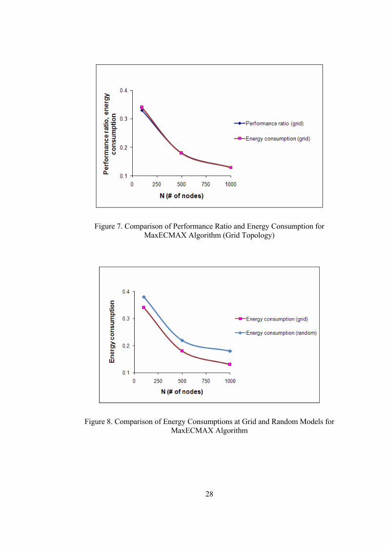
Figure 7. Comparison of Performance Ratio and Energy Consumption for
MaxECMAX Algorithm (Grid Topology)................................................... 28
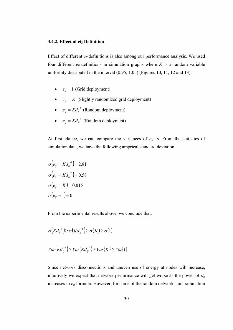
Figure 8. Comparison of Energy Consumptions at Grid and Random Models for
MaxECMAX Algorithm .............................................................................. 28
Figure 9. Total Messages Delivered vs Network Radius for Random Deployment
(N = 500 nodes, eij = Kd4)........................................................................... 29
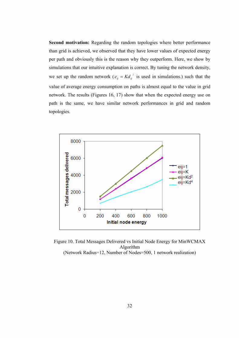
Figure 10. Total Messages Delivered vs Initial Node Energy for MinWCMAX
Algorithm ..................................................................................................... 32
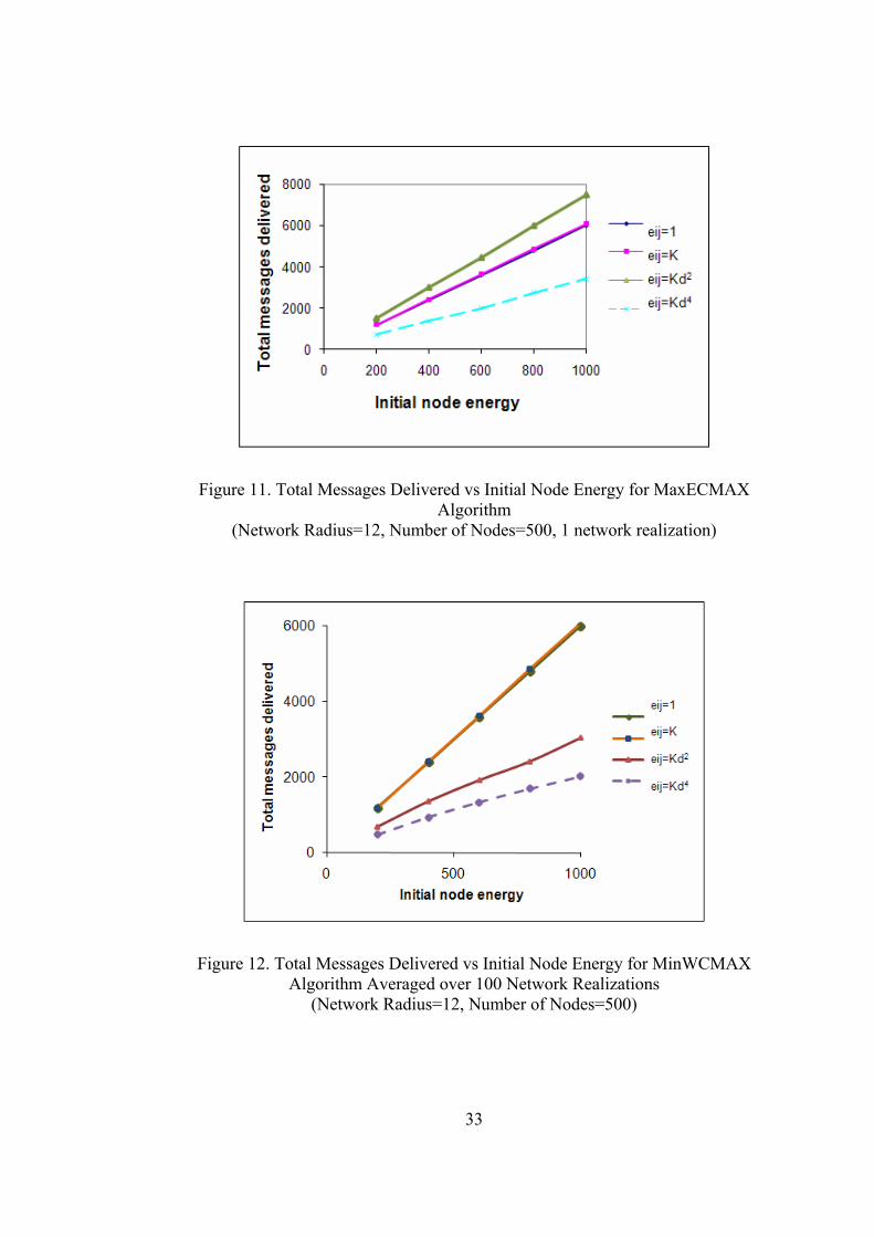
Figure 11. Total Messages Delivered vs Initial Node Energy for MaxECMAX
Algorithm ..................................................................................................... 33
Figure 12. Total Messages Delivered vs Initial Node Energy for MinWCMAX
Algorithm Averaged over 100 Network Realizations.................................. 33
Figure 13. Total Messages Delivered vs Initial Node Energy for MaxECMAX
Algorithm Averaged over 100 Network Realizations.................................. 34
Figure 14. More Investigation on Effect of eij, MinWCMAX Algorithm.................. 34
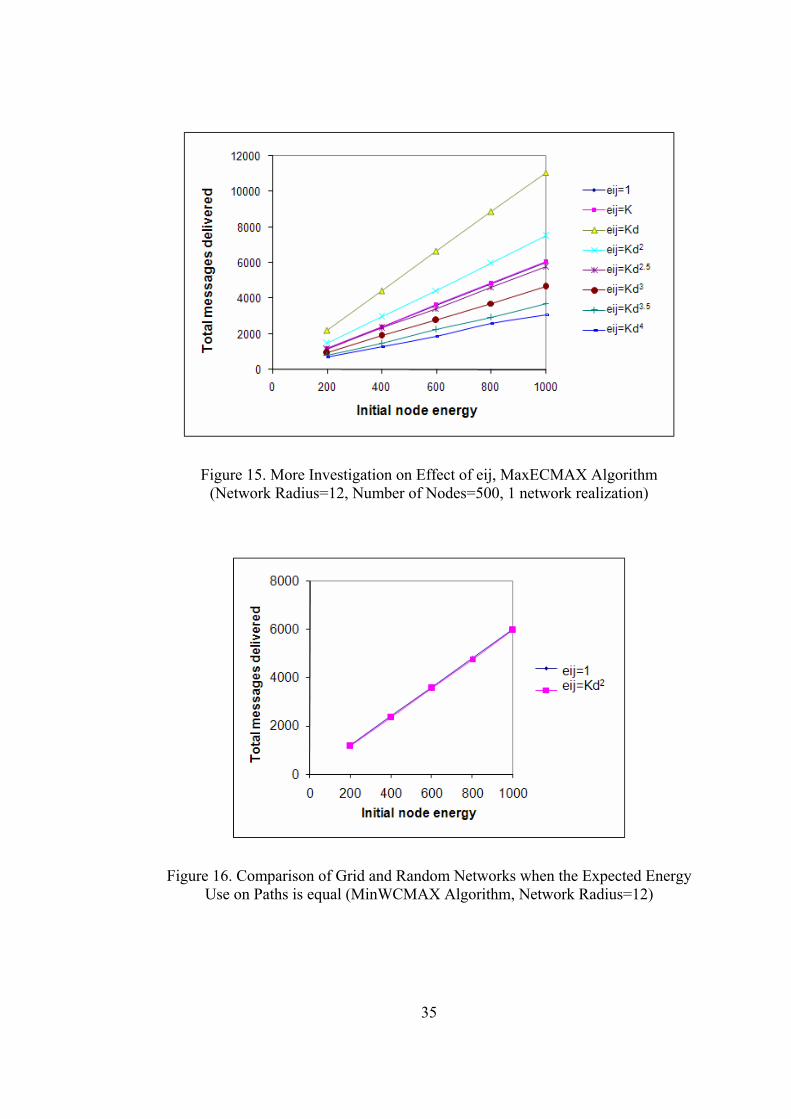
Figure 15. More Investigation on Effect of eij, MaxECMAX Algorithm .................. 35
Figure 16. Comparison of Grid and Random Networks when the Expected Energy
Use on Paths is equal (MinWCMAX Algorithm, Network Radius=12) ..... 35

xii
Figure 17. Comparison of Grid and Random Networks when the Expected Energy
Use on Paths is equal (MaxECMAX Algorithm, Network Radius=12) ...... 36
Figure 18. Network Lifetime vs Initial Node Energy (Random Deployment,
message length is uniformly distributed between (1, 100), Network
Radius=12, Number of Nodes=500) ............................................................ 37
Figure 19. Network Lifetime vs Initial Node Energy (Random Deployment,
message length is uniformly distributed between (50, 100), Network
Radius=12, Number of Nodes=500) ............................................................ 38
Figure 20. Network Lifetime vs Initial Node Energy (Grid Deployment, message
length is uniformly distributed between (1, 100), Network Radius=12,
Number of Nodes=500)................................................................................ 38
Figure 21. Network Lifetime vs Initial Node Energy (Grid Deployment, message
length is uniformly distributed between (50, 100), Network Radius=12,
Number of Nodes=500)................................................................................ 39
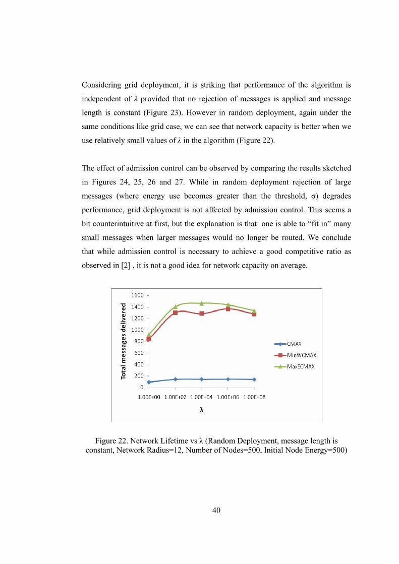
Figure 22. Network Lifetime vs λ (Random Deployment, message length is
constant, Network Radius=12, Number of Nodes=500, Initial Node
Energy=500)................................................................................................. 40
Figure 23. Network Lifetime vs λ (Grid Deployment, message length is constant,
Network Radius=12, Number of Nodes=500, Initial Node Energy=500) ... 41
Figure 24. Network Lifetime vs λ under Admission Control (Random Deployment,
σ = 6205, message length varies between 1-1000, Network Radius=12,
Number of Nodes=500, Initial Node Energy=5000).................................... 41
Figure 25. Network Lifetime vs λ without Admission Control (Random
Deployment, message length varies between 1-1000, Network
Radius=12, Number of Nodes=500, Initial Node Energy=5000) ................ 42
Figure 26. Network Lifetime vs λ under Admission Control (Grid Deployment, σ =
469, message length varies between 1-50, Network Radius=12, Number
of Nodes=500, Initial Node Energy=500).................................................... 42
Figure 27. Network Lifetime vs λ without Admission Control (Grid Deployment,
message length varies between 1-50, Network Radius=12, Number of
Nodes=500, Initial Node Energy=500) ........................................................ 43

xiii
Figure 28. Total Messages Delivered vs Initial Node Energy (Random
Deployment, message length is constant, Network Radius=12, Number of
Nodes=500) .................................................................................................. 44
Figure 29. Total Messages Delivered vs Initial Node Energy (Grid Deployment,
message length is constant, Network Radius=12, Number of Nodes=500). 45
Figure 30. Comparison of Network Lifetime for Different Network Sizes where
network radius R takes the values R=6,12,18 and number of nodes per
unit network area is 1 (Grid Deployment, MaxECMAX Algorithm) .......... 46
Figure 31. Comparison of Network Lifetime for Different Network Sizes where
network radius R takes the values R=6,12,18 and number of nodes per
unit network area n takes the values n=1.00086,1.00086,0.99988
respectively (Random Deployment, MaxECMAX Algorithm) ................... 46

1
CHAPTER I
INTRODUCTION
With advancements in sensor technology, large scale wireless sensor networks
(WSN) are in high demand for various applications [1, 16, 17, 18, 19, 27]. A wide
variety of application fields motivates the dense use of WSNs. In these large and
dense networks, energy efficiency in all protocol layers plays a crucial role for a
sufficiently long network lifetime. Regarding the architecture of the sensor nodes,
we have in mind a small device with limited energy, which is able to communicate
in short distances with low power and limited computing and memory capacities.
Due to these constraints, collaboration of the nodes is fundamentally important.
One place where the need for efficient collaboration is highest is routing [27].
Without an effective routing algorithm, we are likely to have an unpredictable
network capacity and lifetime. What is critical to the success of a large scale
network more than the deployment or the sensing capabilities of devices is a
routing algorithm that considers energy efficiency together with network capacity
maximization [13, 14].
In the rest, we define network capacity as the maximum number of messages that
can be delivered from a given set of senders to a fixed destination node (sink) until
no more messages can be routed in the network. On the other hand, for some parts
of the performance analysis, we also use a different definition for network lifetime,
that is the maximum number of messages that can be delivered until the first failure
of delivery due to insufficient residual energy. Of course, network capacity is not
achievable with a causal (online) routing algorithm, that is, one that does not know
the source nodes of all future packets [2]. For any online algorithm, it is possible to
devise adversarial packet generation sequences that will minimize the lifetime of
the network. Our goal is to obtain a routing algorithm with a good competitive

2
ratio, that is, an online algorithm that performs provably close to network capacity.
We will argue that a routing algorithm should: (i) take into account energy
consumption along paths (ii) mind the remaining energy at nodes along a path (iii)
aggregate similar data to prevent the routing of redundant data1.
WSN routing algorithms reported in the literature may basically be classified into
two: The first class contains energy-centric schemes that focus on routing packets
energy-efficiently through a topology, while being oblivious of the contents of the
packets. Such algorithms can also be regarded as address-centric since they put
emphasis on end-to-end routing between source and destination nodes [20]. These
schemes often use variants of shortest-path routing where path length is a function
of either the energy used on hops, or residual energies at nodes; or both [2, 3, 4, 9,
10, 11, 21, 22, 38]. In the second class, we have data-centric algorithms where data
is well organized with attribute-value pairs and the focus is on data, finding its own
path through the network and getting processed [5, 6, 7, 8, 23, 24].
We observe that neither approach can alone achieve network capacity: Ignoring
residual energies and path energies will lead to wasting energy, or uneven energy
drain, which will lead the network to a suboptimal operating point. On the other
hand, ignoring data similarity will lead to sending redundant data thus wasting
resources again.
Let us briefly examine examples of the first class of routing protocols. Clearly,
minimum hop routing [11] does not necessarily choose energy efficient routes in a
wireless network. Using minimum energy paths [10] tends to result in uneven
energy consumption among nodes, causing early death of the network. A remedy
to the uneven draining problem is to factor the instantaneous residual energies of
nodes in the routing metric [2, 3, 4, 9, 38]. To this end, the approach of Kar et al. in
1 Network coding is beyond the scope of this paper.

3
[2] is remarkable because of the exponential dependence of link weight on the
fraction of used energy of the node at the sending end of the link. The online
algorithm (CMAX) in [2] achieves a logarithmic competitive ratio.
Besides shortest path algorithms referred above, there are some other energy-
centric algorithms as well. [29] aims at delay-aware energy efficiency with the
implementation of a cluster-based algorithm. A simple cost function depending on
link energy use, residual energy and delay parameters is defined in [29] to find the
shortest path within the cluster. Another clustering approach [36] proposes that by
adopting a clustered traffic topology, with additionally deployed router sensors, an
energy efficient routing design can be achieved. Here it is claimed that introducing
extra routers will take over majority of routing burden from sensors. As a different
approach, the algorithm (REAR) in [30] distributes the traffic load evenly in the
network to enable energy efficient routing. On the whole, it is evidently seen that
[29, 30, 36] do not take data fusion into account, which is in fact a must if network
capacity maximization is an objective.
In applications, it is frequently the case that highly correlated data is generated
simultaneously on various nodes. Fusion of collected information is important for
efficient use of resources. This is inherent in the second class of routing protocols,
which are data-centric. Among data-centric algorithms, [23] mentions that
assuming an arbitrary placement of sources in a network graph, the task of doing
data-centric routing with optimal data aggregation is NP-hard. As an alternative
one can propose a Greedy Incremental Tree as a suboptimal solution for data
aggregation. To construct a greedy incremental tree, initially a shortest path is
established for the nearest source to the sink, later each of the other sources is
incrementally connected at the closest point on the existing tree [23, 31].
Besides greedy aggregation, a good example of data-centric routing is directed
diffusion. In directed diffusion, there are attribute-value pairs which describe the
data and enable aggregation. One type of directed diffusion consists of interest

4
broadcast by the sink [5, 7]. To select good paths, gradients with positive or
negative reinforcements are formed as the interest is disseminated through the
network and in this way, the high quality data that best fits the interest attributes is
discovered. Directed diffusion can also be modeled as source-initiated [6, 8]. In
this case, the source broadcasts advertisement of its available data to explore
probable destination nodes that are interested. Hence, either source or destination is
unknown in directed diffusion and decided via established gradients. Here, a
network with unknown destination is often not a practical model. In practice, there
is usually a single sink at the center of the network collecting information from
other sensors.
Moreover, in data centric algorithms, the sink tries to find the path with fastest data
rate (high quality data) [5] and this implies the frequent use of specific paths which
will result in running out of energy rapidly on these paths and losing the associated
nodes. If there is no interest match, data message at the node is silently dropped. In
some cases, the data produced at a node may need to be urgently sent to the sink.
For sink-initiated situations, sometimes there might be an interest where there are
no matching nodes, which will mean redundant energy use for interest diffusion
and gradient establishment. If quick response to the requests of the sink is the
primary goal, directed diffusion can be a good solution. It is evident that it is not
suited to maximizing capacity under energy constraints.
Apart from those two main classes that have been referred above, there are some
energy considering routing algorithms with data aggregation as well. Such
algorithms can also be classified into two: routing-driven algorithms and
aggregation-driven algorithms. While the routing-driven are focused on minimum
weight routing path by also regarding data aggregation [15, 25, 26, 37], the
aggregation-driven are primarily focused on data processing and secondly give
importance to energy consumption [7, 28, 33, 34, 35].
5
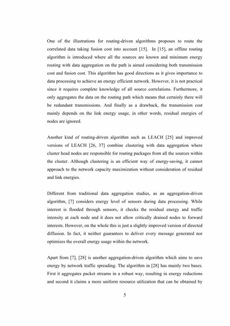
One of the illustrations for routing-driven algorithms proposes to route the
correlated data taking fusion cost into account [15]. In [15], an offline routing
algorithm is introduced where all the sources are known and minimum energy
routing with data aggregation on the path is aimed considering both transmission
cost and fusion cost. This algorithm has good directions as it gives importance to
data processing to achieve an energy efficient network. However, it is not practical
since it requires complete knowledge of all source correlations. Furthermore, it
only aggregates the data on the routing path which means that certainly there will
be redundant transmissions. And finally as a drawback, the transmission cost
mainly depends on the link energy usage, in other words, residual energies of
nodes are ignored.
Another kind of routing-driven algorithm such as LEACH [25] and improved
versions of LEACH [26, 37] combine clustering with data aggregation where
cluster head nodes are responsible for routing packages from all the sources within
the cluster. Although clustering is an efficient way of energy-saving, it cannot
approach to the network capacity maximization without consideration of residual
and link energies.
Different from traditional data aggregation studies, as an aggregation-driven
algorithm, [7] considers energy level of sensors during data processing. While
interest is flooded through sensors, it checks the residual energy and traffic
intensity at each node and it does not allow critically drained nodes to forward
interests. However, on the whole this is just a slightly improved version of directed
diffusion. In fact, it neither guarantees to deliver every message generated nor
optimizes the overall energy usage within the network.
Apart from [7], [28] is another aggregation-driven algorithm which aims to save
energy by network traffic spreading. The algorithm in [28] has mainly two bases.
First it aggregates packet streams in a robust way, resulting in energy reductions
and second it claims a more uniform resource utilization that can be obtained by

6
shaping the traffic flow. Although [28] will surely outperform pure data
aggregation, it still cannot offer a solution close to the optimal case since it
disregards energy efficient path selection. On the other hand, [33, 34, 35] give
importance to the optimization of data aggregation cost. They simply try to
implement minimum energy data gathering by considering different coding
techniques. Here, again no value is given to the energy efficient routing, only
energy saving during the aggregation is considered. Moreover, in these algorithms,
it is assumed that information sources supply a constant amount of information,
which is far from the practical case.
In this thesis, our goal is to combine the strengths of the first and second classes of
protocols. This can be viewed as a preliminary study toward proposing a new
routing algorithm. In our search for the holy grail of a provably competitive routing
algorithm, we start with what we know is very competitive in the first class, the
CMAX [2] algorithm, and explore how it performs under data aggregation.
The outline of the rest of the thesis is as follows. In Chapter II , the network model
and the modified CMAX algorithm are described. In Chapter III, the performance
of this algorithm is considered. While implementation issues are discussed in
Chapter IV, conclusion remarks and further directions are given in Chapter V and
VI respectively.
7
CHAPTER II
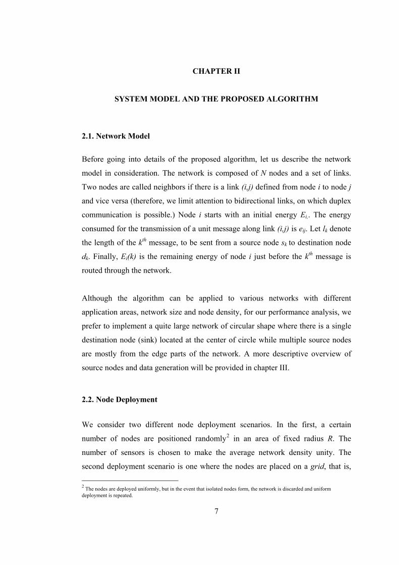
SYSTEM MODEL AND THE PROPOSED ALGORITHM 2.1. Network Model
Before going into details of the proposed algorithm, let us describe the network
model in consideration. The network is composed of N nodes and a set of links.
Two nodes are called neighbors if there is a link (i,j) defined from node i to node j
and vice versa (therefore, we limit attention to bidirectional links, on which duplex
communication is possible.) Node i starts with an initial energy Ei,. The energy
consumed for the transmission of a unit message along link (i,j) is eij. Let lk denote
the length of the kth message, to be sent from a source node sk to destination node
dk. Finally, Ei(k) is the remaining energy of node i just before the kth message is
routed through the network.
Although the algorithm can be applied to various networks with different
application areas, network size and node density, for our performance analysis, we
prefer to implement a quite large network of circular shape where there is a single
destination node (sink) located at the center of circle while multiple source nodes
are mostly from the edge parts of the network. A more descriptive overview of
source nodes and data generation will be provided in chapter III.
2.2. Node Deployment
We consider two different node deployment scenarios. In the first, a certain
number of nodes are positioned randomly2 in an area of fixed radius R. The
number of sensors is chosen to make the average network density unity. The
second deployment scenario is one where the nodes are placed on a grid, that is,
2 The nodes are deployed uniformly, but in the event that isolated nodes form, the network is discarded and uniform deployment is repeated.
8
equidistant from each of their neighbors (hexagonal node placement), inside the
circle of radius R.
We let the energy consumed per unit-length message on link (i,j) be given by 4
ijij Kde = where dij is the distance between nodes i and j, and K is a random
scaling coefficient, crudely modeling channel fading. K is uniformly distributed
between (0.95, 1.05). We let eij = eji and say that i and j are neighbors if eij is
smaller than a certain threshold value. We choose the threshold value such that
every node in the network has at least one neighbor.
In random deployment scenario, in order to observe the performance differences,
we also tried dij2 to calculate eij values.
The grid deployment scenario is an idealization, with distances to all neighbors
being unity. We go one step further and set 1=K so that in the grid model,
1== ijij de .
Now, we provide a proof-of-concept algorithm, under highly idealized assumptions
about centralized control, ideal fusion of information that will make our
observation about combining classes and related tradeoffs concrete.
2.3. The Algorithm
Before introducing our proposed algorithm, let us first describe CMAX algorithm
[2] which forms a basis for our design since shortest path is calculated exactly in
the same manner as CMAX.

9
2.3.1. CMAX Algorithm
Routing objective of CMAX is to maximize the total number of messages that can
be successfully sent over the network (network capacity) without knowing any
information regarding future message arrivals or message generation rates. The
algorithm uses knowledge of residual battery energy at each node, and also
considers the straightforward setting where energy consumption for message
transmission, i.e., eij depends on the distance to the neighbor. It is showed in [2]
that if admission control of messages is allowed, the algorithm achieves a
competitive ratio that is logarithmic in the number of network nodes, i.e., its
performance without knowledge of future message arrivals is in the worst case
within a logarithmic factor of the best performance achievable by an off-line
algorithm with complete information about messages to be transmitted. Admission
control is defined as rejecting to deliver a message when the total length of the
shortest path is greater than a defined threshold value, σ. It is proved in [2] that
maxne =σ , where emax is the maximum energy expended on some link in the
network by a unit-length message, is the best choice to have the logarithmic
competitive ratio. In general, there are two cases where admission control is
applied. In the first case, due to the insufficient residual energies at some
intermediate nodes, the message can only be routed through a long path of many
hops, which significantly increases the total cost. On the other hand, evidently the
second case is when the message length is too big to pass the threshold σ and be
routed.
CMAX follows these steps:
1. Consider routing message k on the network G. Eliminate all links, (i,j), in the
network for which residual energy is insufficient, that is ( ) ijki elkE ⋅< to form a
reduced network.

10
2. Associate weights wij with each link (i,j) in the reduced graph, where
( ) )1−=k
ijiji( ew α
λ
3. Find the shortest path from sk to dk in the reduced graph with link weights wij,
as defined in Step 2.
4. Let γk be the length of the shortest path found in Step 3 ( ∞=kγ if no path was
found). If σγ ≤k , route the message along the shortest path, otherwise reject it.
Above, ( ) ( )i
ii E
kEk −= 1α is the fraction of the initial energy of node i that has been
used by the time the kth message arrives. λ is a constant and in [2], it is proved that
selecting )1(2min
max +=eeNλ gives the best competitive ratio (emax and emin are
respectively the maximum and minimum energies expended on some link in the
network by a unit-length message.). Note that step 1 is applied to reduce the
complexity of the algorithm.
From the weight definition of the algorithm, it can be seen that the weight of a link
(i,j), wij, increases with an increase in eij, the energy expended in traversing link
(i,j). Moreover, wij increases as the energy utilization of the transmitting node,
( )kiα increases. This means that the algorithm tries to avoid links which require
very high energy for transmission, and nodes where the residual energy fraction is
low. Furthermore, as we have the same constant eij’s in use along the whole
network lifetime, the dynamic variable ( )kiα is the principal factor affecting the
weight function. Therefore, it has exponential dominancy in the formula.
2.3.2. Modified CMAX Algorithm:
The modified version of the algorithm that we propose in this thesis is as follows:

11
For the kth event Evk (We define any instant producing data to be delivered to the
sink as an event.),
1. Form a reduced network by eliminating all links, i,j, in the network for which
residual energy is insufficient, that is ( ) ijki elkE ⋅<
2. Form the set kS (the set of source nodes for messages k that is produced by
Evk)
3. For all kSi∈ , find ∑∈
=*
ipj
jki wW where pi is the set of nodes on a path from
source i to the sink and ∑∈
=ipkj
jkipi wp),(
* minarg . Link weight for wjk is defined
as ( ) )1−=k
jkjkj( ew α
λ .
4. From the set kS , select ii Wi minarg=
5. Deliver the message on the minimum weight path from selected source i to the
sink and update the residual energies accordingly.
6. Return step 1 to deliver another event.
Different from CMAX, our algorithm does not apply admission control. We think
that practically admission control should not be used. Since it prevents the delivery
of some messages, it is very probable that some critical data cannot be routed to the
sink, although there is enough residual energy at nodes.
On the other hand we can elaborate the significance of our modification as follows:
If a group of sensors are activated due to the same event, the message produced by
this event is delivered by only one of the sensors in the group, i.e., set kS . Hence re-
transmissions of the same message to the sink are prevented. Our algorithm uses
two different approaches to form kS . First is the theoretical approach
(MinWCMAX) where all sources effected by the Evk are included in kS . Here, all
minimum weight paths are calculated from the sources with data of the same event
and then only the source that has the minimum of all calculated path weights sends

12
the message. Since this algorithm requires complete knowledge of calculated paths,
it is not feasible to implement it in real life; it provides theoretically best results
though. In our second approach (MaxECMAX), that is more practical, only the
source node with the maximum residual energy is included in kS . Thus, here the
minimum weight path is calculated only for a single node in kS , i.e., the source
node having the maximum residual energy. Some discussion about how to
practically select the node with maximum residual energy is given in chapter IV.

13
CHAPTER III
PERFORMANCE ANALYSIS
We consider a scalable circular network with a single, fixed destination node,
namely sink, located at the center and we assume messages are generated mainly
from edges of the network. The underlying scenario for this assumption is as
follows: We would like to observe the performance improvement in a network
where the objective is intruder detection at the boundaries of the network. Beyond
this scenario, the algorithm can be implemented for a network where any node can
be potentially source or destination. Moreover, although simulations were based on
unit node density on average, the algorithm can easily handle scalability issues and
perform well in larger or more densely deployed networks.
On the other hand, since we mainly focus on the effect of data fusion on an energy
constrained algorithm, we both theoretically and practically aim to prove its vitality
and disregard potentially important implementation issues. First, we do not model
all possible types of energy losses, but we simply accept that the only energy
consumption at a node is due to packet transmission to the next hop. Energy losses
at packet receptions are assumed to be included in transmission losses as all nodes
on a path have both transmission and reception phases except source and
destination [2]. Second, the algorithm requires knowledge of network topology and
up-to-date energy levels at the nodes. Though in chapter IV some implementation
alternatives are proposed to cope with those practical issues, a concrete solution is
beyond the scope of this thesis and obviously considered to be future work.
We shall make use of simulations to aid in our understanding of the performance of
the routing algorithm described in the previous section. Particularly, we would like
to draw attention to the key role that early data aggregation near the generated
events (data aggregation at the sources) plays in saving energy [31, 32].
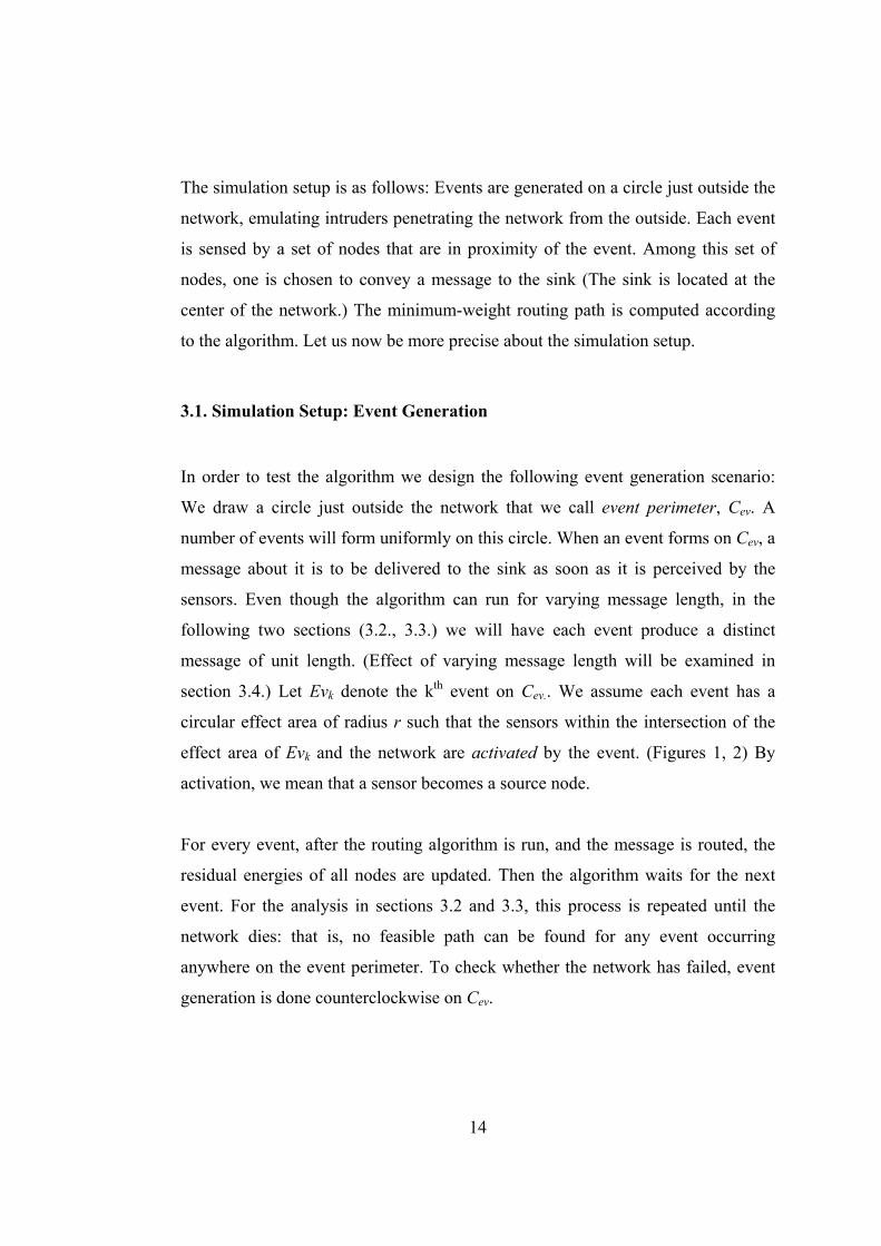
14
The simulation setup is as follows: Events are generated on a circle just outside the
network, emulating intruders penetrating the network from the outside. Each event
is sensed by a set of nodes that are in proximity of the event. Among this set of
nodes, one is chosen to convey a message to the sink (The sink is located at the
center of the network.) The minimum-weight routing path is computed according
to the algorithm. Let us now be more precise about the simulation setup.
3.1. Simulation Setup: Event Generation
In order to test the algorithm we design the following event generation scenario:
We draw a circle just outside the network that we call event perimeter, Cev. A
number of events will form uniformly on this circle. When an event forms on Cev, a
message about it is to be delivered to the sink as soon as it is perceived by the
sensors. Even though the algorithm can run for varying message length, in the
following two sections (3.2., 3.3.) we will have each event produce a distinct
message of unit length. (Effect of varying message length will be examined in
section 3.4.) Let Evk denote the kth event on Cev.. We assume each event has a
circular effect area of radius r such that the sensors within the intersection of the
effect area of Evk and the network are activated by the event. (Figures 1, 2) By
activation, we mean that a sensor becomes a source node.
For every event, after the routing algorithm is run, and the message is routed, the
residual energies of all nodes are updated. Then the algorithm waits for the next
event. For the analysis in sections 3.2 and 3.3, this process is repeated until the
network dies: that is, no feasible path can be found for any event occurring
anywhere on the event perimeter. To check whether the network has failed, event
generation is done counterclockwise on Cev.

15
In the simulations of this chapter, we continue to generate events and send
messages until the network entirely dies (in order to approximate network
capacity). It is explicitly mentioned wherever a different network lifetime
definition is used. There is a separate section (3.4) where different network lifetime
definitions are compared. Similarly unless explicitly stated, we use a constant
message length of 10 units and average values over 100 network realizations are
simulated for random networks.
Figure 1. Event Generation in Random Deployment
16
Figure 2. Event Generation in Grid Deployment
3.2. Comparison of MinWCMAX and MaxECMAX Algorithms
Before going into details of performance analysis, we would like to make a
comparison between our two proposed algorithms, MinWCMAX and
MaxECMAX.
We propose MinWCMAX as an ideal theoretical solution since it searches through
all the possible paths and really selects the minimum weight path for an event.
However, practically it is difficult to implement and besides, has a high
computational complexity. The complexity of MinWCMAX algorithm introduces
two main problems when implementation is considered: a possibly large delay
until a path decision is made and energy consumed in computation (processing).
As we will see, MaxECMAX proves to be a good promise in terms of complexity
and feasibility. MaxECMAX lets the node with maximum instantaneous energy to
send the information of an event on behalf of all sources with the same data. For
random node deployment, we expect that MaxECMAX algorithm will not
17
necessarily be as successful as MinWCMAX in choosing the minimum weight
path to deliver the event from a selected source. However, for networks with grid
topology, this is not true. In grid topology, since all the distances and eij values
between neighbors are unity, link energy usage is not a factor in the weight
calculation, i.e., residual energy is the only factor. Concerning this fact, in grid
mode, MaxECMAX meets the requirements of the weight definition, thus provides
the same network performance like MinWCMAX.
All simulation experiments in this thesis included both MinWCMAX and
MaxECMAX. They illustrate the competitive performance of MaxECMAX
algorithm for both random and grid network topologies.
3.3. An Analytical Base for Simulations
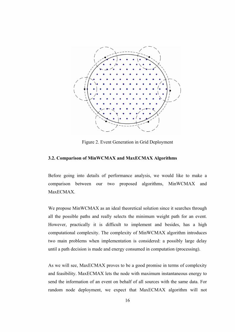
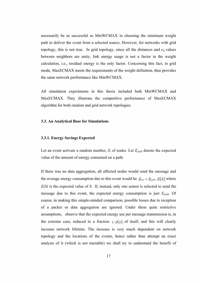
3.3.1. Energy Savings Expected
Let an event activate a random number, S, of nodes. Let Epath denote the expected
value of the amount of energy consumed on a path.
If there was no data aggregation, all affected nodes would send the message and
the average energy consumption due to this event would be ( )SEEE pathuse ⋅= where
E(S) is the expected value of S. If, instead, only one sensor is selected to send the
message due to this event, the expected energy consumption is just Epath. Of
course, in making this simple-minded comparison, possible losses due to reception
of a packet or data aggregation are ignored. Under these quite restrictive
assumptions, observe that the expected energy use per message transmission is, in
the extreme case, reduced to a fraction ( )SE/1 of itself, and this will clearly
increase network lifetime. The increase is very much dependent on network
topology and the locations of the events, hence rather than attempt an exact
analysis of it (which is not tractable) we shall try to understand the benefit of
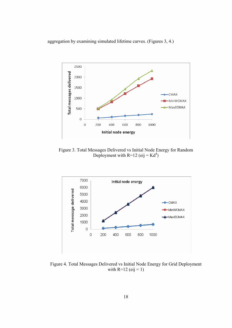
18
aggregation by examining simulated lifetime curves. (Figures 3, 4.)
Figure 3. Total Messages Delivered vs Initial Node Energy for Random Deployment with R=12 (eij = Kd4)
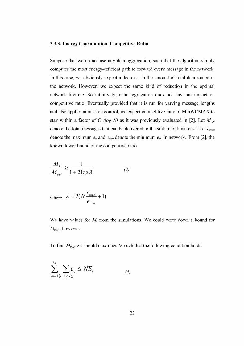
Figure 4. Total Messages Delivered vs Initial Node Energy for Grid Deployment
with R=12 (eij = 1)

19
Let the average area of the intersection of an event effect circle with the network
be Acommon. The average number of nodes activated by an event is proportional to
this area. A first order estimate of ( )SE can thus be found as
NA
AS
N
common ⋅= (1)
Let δ denote the ratio of slope of MaxECMAX to slope of CMAX in Figures 3 and
4. The comparison of δ and S is as follows:
Table I - Comparison of Theoretical and Simulated Gain of Data Aggregation
Grid Random Network Size
δ S δ S
R=6 (N=100) 10.4 10.7 6.8 10.7
R=12 (N=500) 8.8 11.1 7.9 11.1
R=18 (N=1000) 5.5 9.6 9.1 9.6
Comparison of values above suggests that random deployment is not as reliable as
grid deployment, since the variance of eij’s is higher. Furthermore, the aggregation
benefit δ closely follows S in the grid network at small network sizes.
3.3.2. More on the Grid Topology
Let Mt be the practically observed total number of distinct messages successfully
delivered to the sink in a simulation instance. Figures 3, 4 and 5 plot Mt vs initial
node energy, Ei. Let ηp denote the slope of these experimental plots. We would like
to understand the reliability of the simulated (practical) slope ηp. To this end, let ηt
denote the expected (theoretical) slope, using the MaxECMAX algorithm.

20
Let the theoretical corresponding of Mt be ~
Mt and is defined with the following
modelling:
∑=
=
Δ
H
1hh
i
e
N EMt~
where eh is the energy used on hop h for the transmission of a randomly chosen
packet, for which the total number of hops on a path is a random number H.
Then ηt is:
⎟⎟⎟⎟
⎠
⎞
⎜⎜⎜⎜
⎝
⎛
∑⎟⎟⎟
⎠
⎞
⎜⎜⎜
⎝
⎛
∑=
⎟⎟⎟
⎠
⎞
⎜⎜⎜
⎝
⎛=
==
=H
1hh
i
iH
1hh
i
iit
eH1
H
N EE1
Ee
N EE1
EE
EMt
~
η (2)
As the value of H gets large, we can approximate ∑=
H
1h heH1
by a constant, but in
general this is a random variable T. Hence, (2) becomes
)(HTEN
HTN
Et ≤⎟⎠⎞
⎜⎝⎛=η
where the last inequality is from Jensen’s Inequality.
Proposition 1: For a given expected energy per path, )(HTE , holding the equality,
grid topology maximizes the slope tη , which suggests that the network capacity is
maximized in the grid topology.

21
Above, equality is achieved when the product HT is deterministic. In general, path
energy in the network is not deterministic and within network lifetime it changes
depending on the path length and the link energies on the path. However for grid
topology, since all link energies and initial node energies are identical, we expect
that path length H stays the same provided that residual energy is sufficient at
nodes. Disregarding the longer paths that are formed toward the end of network
lifetime (due to insufficient residual energies at mostly used nodes close to the
sink), a constant HT value will be kept throughout the duration of interest as we are
observing the creation and sending of messages in the grid topology (The value of
T is already a constant by definition in the grid.)
Moreover, simulations support that path length H is the same for all message
deliveries as long as there is sufficient energy at nodes.
Comparison of ηp values in Figure 5 supports Proposition 1.
Figure 5. Total Messages Delivered vs Initial Node Energy for MaxECMAX algorithm with R=12
22
3.3.3. Energy Consumption, Competitive Ratio
Suppose that we do not use any data aggregation, such that the algorithm simply
computes the most energy-efficient path to forward every message in the network.
In this case, we obviously expect a decrease in the amount of total data routed in
the network. However, we expect the same kind of reduction in the optimal
network lifetime. So intuitively, data aggregation does not have an impact on
competitive ratio. Eventually provided that it is run for varying message lengths
and also applies admission control, we expect competitive ratio of MinWCMAX to
stay within a factor of O (log N) as it was previously evaluated in [2]. Let Mopt
denote the total messages that can be delivered to the sink in optimal case. Let emax
denote the maximum eij and emin denote the minimum eij in network. From [2], the
known lower bound of the competitive ratio
λlog211
+≥
opt
t
MM
(3)
where )1(2min
max +=eeNλ
We have values for Mt from the simulations. We could write down a bound for
Mopt , however:
To find Mopt, we should maximize M such that the following condition holds:
( )i
M
m Pjiij NEe
m
≤∑ ∑= ∈1 ,
(4)
23
where Pm is the shortest path on which the mth message is routed. We assume that
messages are generated on the perimeter of the network in order to have almost a
uniform Pm for the ease of analysis. The values of eij’s and Pm are selected
according to the graph constraints.
Conjecture 1: M is maximized in (4) when eeij = ji,∀ and hPm = m∀ where e
and h are constants.
Moreover, as a very loose bound, we know that minmineh
NEM i≤ where hmin is the
minimum mP .
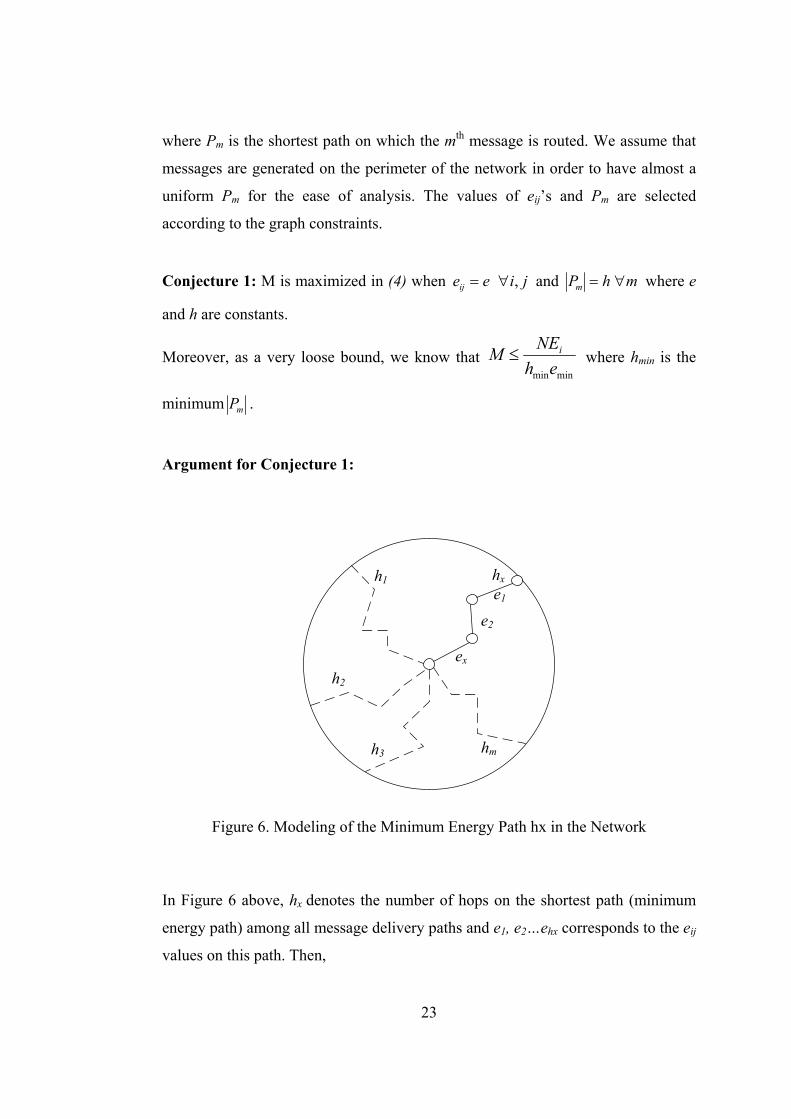
Argument for Conjecture 1:
h1 hx
ex
h2
h3 hm
e1
e2
Figure 6. Modeling of the Minimum Energy Path hx in the Network
In Figure 6 above, hx denotes the number of hops on the shortest path (minimum
energy path) among all message delivery paths and e1, e2…ehx corresponds to the eij
values on this path. Then,
24
∑=
≤xh
ii
i
e
NEM
1
(5)
where ∑=
xh
iie
1 is the total energy used to route the xth message to the sink on the
shortest path Px.
In (5), ∑=
xh
ii
i
e
NE
1
is convex in ei’s. Then by convexity, choosing eei = ie∀ will
minimize the expression ∑=
xh
iie
1, hence will maximize the right hand side of the
inequality.
Corollary of Conjecture 1:
Making use of the expression (5) we propose the following lower bound for the
optt MM / ratio:
∑=
≥
xh
ii
i
t
opt
t
e
NEM
MM
1
(6)
Consequently, from (3) and (6) we have two different lower bounds on the ratio,
optt MM / .
25
Let the theoretical lower bound on optt MM / in (3) be ( )minmax ,, eeNBt , so we have
( )λlog21
1,, minmax +=eeNBt
And let the practical lower bound on optt MM / be ( )graphBp , so similarly we have
( )
∑=
=
xh
ii
i
tp
e
NEMgraphB
1
We can make use of the comparison of these two lower bounds. If
( ) ( )minmax ,, eeNBgraphB tp < holds, our intuitive bound is useless, and otherwise,
it is an improvement over the theoretical competitive bound. So, we can use
( ) ( ){ }minmax ,,, eeNBgraphBMax tp to define the resultant lower bound for the
performance ratio of our algorithm. Performance ratio is defined as the ratio of
network lifetime under MaxECMAX algorithm to the optimal network capacity.
Note that optt MM / represents the performance ratio.
Table II shows that our simulation results are very close to the bound in (3) (Figure
7). This result suggests that our conjecture for the lower bound on performance
ratio, i.e., ( )graphBp is a good, consistent modeling. Moreover, since [2] applies
admission control to propose the bound ( )minmax ,, eeNBt , but we do not apply it and
accept every length of message generated, it is in fact foreseeable that our proposed
lower bound is smaller than the theoretical lower bound in (3). In the analysis
given at Table II, for all network sizes, 1200 =tM for grid network model and
650 ≈tM for random network model.

26
Table II - Comparison of Theoretical Lower Bound and Practical Lower Bound on
Performance Ratio for Different Network Sizes and Deployment Models
Grid Random Network
Size (N) ( )graphBp ( )minmax ,, eeNBt ( )graphBp ( )minmax ,, eeNBt
N=100 0.19 0.19 0.09 0.12
N=500 0.13 0.16 0.07 0.10
N=1000 0.10 0.13 0.06 0.08
Let μ denote the energy consumption of network which is defined as the ratio of
total energy use of network within its lifetime to the total initial energy. Since for
grid deployment, we have eij of zero variance and H with small variance, assuming
that eij and H are independent and identically distributed random variables, we can
have the following simplified expression for the grid topology:
( ) ( )ij
iopt eEHE
EN M
⋅= (7)
Here in grid network, ( ) 1=ijeE and disregarding longer paths formed toward the
end of network lifetime, ( ) =HE constant = C:
C
ENi
opt M⋅
= (8)
which is also equal to the ~
Mt (theoretical definition for total number of messages
delivered within network lifetime) that is defined in section 3.3.2.
27
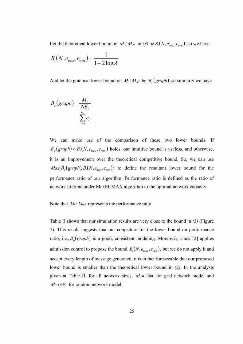
We conclude with the following table when Mt / Mopt values are calculated (based
on simulation results) according to (8) and compared with energy consumption:
Table III - Comparison of Performance Ratio and Energy Consumption for Grid Topology
Network Size (N) Mopt
Mt μ
N=100 0.33 0.34
N=500 0.18 0.18
N=1000 0.13 0.13
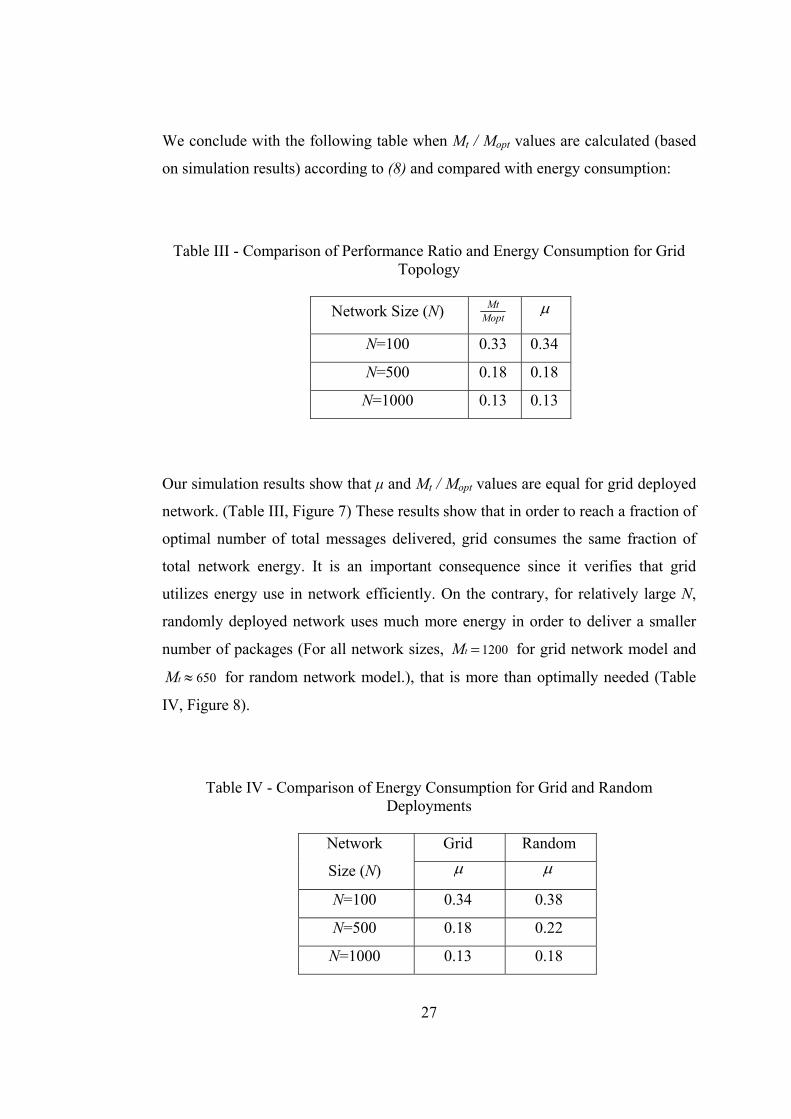
Our simulation results show that μ and Mt / Mopt values are equal for grid deployed
network. (Table III, Figure 7) These results show that in order to reach a fraction of
optimal number of total messages delivered, grid consumes the same fraction of
total network energy. It is an important consequence since it verifies that grid
utilizes energy use in network efficiently. On the contrary, for relatively large N,
randomly deployed network uses much more energy in order to deliver a smaller
number of packages (For all network sizes, 1200 =tM for grid network model and
650 ≈tM for random network model.), that is more than optimally needed (Table
IV, Figure 8).
Table IV - Comparison of Energy Consumption for Grid and Random Deployments
Grid Random Network
Size (N) μ μ
N=100 0.34 0.38
N=500 0.18 0.22
N=1000 0.13 0.18
28
Figure 7. Comparison of Performance Ratio and Energy Consumption for MaxECMAX Algorithm (Grid Topology)
Figure 8. Comparison of Energy Consumptions at Grid and Random Models for MaxECMAX Algorithm

29
3.4. Effect of Different Parameters on Simulations
3.4.1. Effect of Network Density
One of the observations we have made during simulations is the effect of network
density on network capacity. We keep the number of nodes (N=500) constant and
change the network density by changing the radius of network, i.e., network area.
Simulation results show that while CMAX algorithm is not affected much by
network density, MaxECMAX algorithm considerably performs better as node
density increases (Figure 9). Consequently, an important issue to mention is that
due to the increase in number of nodes affected by a specific event, aggregation
becomes crucial and inevitably necessary in densely deployed networks. (Figure 9)
Figure 9. Total Messages Delivered vs Network Radius for Random Deployment (N = 500 nodes, eij = Kd4)
30
3.4.2. Effect of eij Definition
Effect of different eij definitions is also among our performance analysis. We used
four different eij definitions in simulation graphs where K is a random variable
uniformly distributed in the interval (0.95, 1.05) (Figures 10, 11, 12 and 13):
• 1=ije (Grid deployment)
• Keij = (Slightly randomized grid deployment)
• 2
ijij Kde = (Random deployment)
• 4ijij Kde = (Random deployment)
At first glance, we can compare the variances of eij ‘s. From the statistics of
simulation data, we have the following amprical standard deviation:
( ) 81.24 == ijij Kdeσ
( ) 58.02 == ijij Kdeσ
( ) 015.0== Keijσ
( ) 01 ==ijeσ
From the experimental results above, we conclude that:
( ) ( ) ( ) ( )124 σσσσ ≥≥≥ KKdKd ijij
{ } { } { } { }124 VarKVarKdVarKdVar ijij ≥≥≥
Since network disconnections and uneven use of energy at nodes will increase,
intuitively we expect that network performance will get worse as the power of dij
increases in eij formula. However, for some of the random networks, our simulation

31
graphs show different results. Observing one of the sample networks that we used
in Figures 10 and 11, we can see that unexpectedly 2
ijij Kde = outperforms of all.
We can explain this result as follows: We observed that { } 7.12 ≈= ijij KdeAvg , that
is not a very high value, for the network in Figures 10 and 11. Moreover, in
random deployment, initially the paths with small eij values are densely used,
which may explain the surprising performance difference in simulations. But
evidently 4
ijij Kde = has the worst performance since the { } 4.44 ≈= ijij KdeAvg ,
which is quite high making the disconnection problem dominant.
On the other hand, considering performance graphs based on average values over
100 trials, (Figures 12 and 13), the results are as expected for both MinWCMAX
and MaxECMAX algorithms. The performance gets worse with the increase in eij
variance.
Better network performance in some cases under 2
ijij Kde = motivated us to make
further investigation:
First motivation: We searched for a threshold value where grid topology beats
random topology as variance of eij increases. Figures 14 and 15 show that while
ijij Kde = and 2
ijij Kde = performs better than grid case ( 1=ije and Keij = ),
5.2
ijij Kde = has almost the same performance as the grid. Others
( 3
ijij Kde = , 5.3
ijij Kde = and 4
ijij Kde = ) get worse as the power of distance ( ijd )
gets larger in the formula. From Figures 14 and 15, we conclude that grid performs
better for the values greater than 5.2
ijd . An attenuation that has a power law of 2 is
attainable only in free space, and for terrestrial networks, a power larger than 2.5 is
expected, making the result about the superiority of grid topology relevant for all
practical purposes.
32
Second motivation: Regarding the random topologies where better performance
than grid is achieved, we observed that they have lower values of expected energy
per path and obviously this is the reason why they outperform. Here, we show by
simulations that our intuitive explanation is correct. By tuning the network density,
we set up the random network ( 2
ijij Kde = is used in simulations.) such that the
value of average energy consumption on paths is almost equal to the value in grid
network. The results (Figures 16, 17) show that when the expected energy use on
path is the same, we have similar network performances in grid and random
topologies.
Figure 10. Total Messages Delivered vs Initial Node Energy for MinWCMAX Algorithm
(Network Radius=12, Number of Nodes=500, 1 network realization)
33
Figure 11. Total Messages Delivered vs Initial Node Energy for MaxECMAX Algorithm
(Network Radius=12, Number of Nodes=500, 1 network realization)
Figure 12. Total Messages Delivered vs Initial Node Energy for MinWCMAX Algorithm Averaged over 100 Network Realizations
(Network Radius=12, Number of Nodes=500)

34
Figure 13. Total Messages Delivered vs Initial Node Energy for MaxECMAX Algorithm Averaged over 100 Network Realizations
(Network Radius=12, Number of Nodes=500)
Figure 14. More Investigation on Effect of eij, MinWCMAX Algorithm (Network Radius=12, Number of Nodes=500, 1 network realization)
35
Figure 15. More Investigation on Effect of eij, MaxECMAX Algorithm (Network Radius=12, Number of Nodes=500, 1 network realization)
Figure 16. Comparison of Grid and Random Networks when the Expected Energy Use on Paths is equal (MinWCMAX Algorithm, Network Radius=12)

36
Figure 17. Comparison of Grid and Random Networks when the Expected Energy Use on Paths is equal (MaxECMAX Algorithm, Network Radius=12)
3.4.3. Effect of Varying Message Length
As well as constant message length, we also performed simulations with varying
message length. We consider two different cases:
1. Message length is a random variable uniformly distributed in the
interval (1, 100)
2. Message length is a random variable uniformly distributed in the
interval (50, 100)
For random deployment, comparing Figures 18 and 19, we can see that we can
obtain more stable results when the message lengths are varying from very small
values to the very large values. Although the overall variance of message length is
smaller in Figure 19, we get worse performance since the average length of
messages is quite large compared to Figure 18. However, it is also apparent that
our proposed algorithms MinWCMAX and MaxECMAX are more robust to big
message lengths compared to the CMAX algorithm (Figure 19).

37
For random deployment, another important observation is that all of the algorithms
(CMAX, MinWCMAX, MaxECMAX) performs better when the performance is
compared with the case of constant message length. (Figures 3, 18 and 19) This is
an encouraging result since in practice usually we have both random node
distribution and random message length.
Regarding grid deployment, network capacity is completely robust to the changes
in message lengths, message length is either constant or varying, we get almost the
same results when the network is deployed in grid topology. (Comparison of
Figures 3, 20 and 21). This is a good result since it shows that our routing
algorithm is independent of message length provided that too big messages are not
sent causing an initial failure of delivery due to insufficient energy at nodes.
Figure 18. Network Lifetime vs Initial Node Energy (Random Deployment, message length is uniformly distributed between (1, 100), Network Radius=12,
Number of Nodes=500)

38
Figure 19. Network Lifetime vs Initial Node Energy (Random Deployment, message length is uniformly distributed between (50, 100), Network Radius=12,
Number of Nodes=500)
Figure 20. Network Lifetime vs Initial Node Energy (Grid Deployment, message length is uniformly distributed between (1, 100), Network Radius=12, Number of
Nodes=500)

39
Figure 21. Network Lifetime vs Initial Node Energy (Grid Deployment, message length is uniformly distributed between (50, 100), Network Radius=12, Number of
Nodes=500)
3.4.4. Effect of λ
We observed effect of λ from many points of view:
• In Grid Network Deployment:
o Where message length is constant
o Where message length is varying and no admission control is
applied.
o Where message length is varying and admission control is
applied.
• In Random Network Deployment:
o Where message length is constant
o Where message length is varying and no admission control is
applied.
o Where message length is varying and admission control is
applied.
40
Considering grid deployment, it is striking that performance of the algorithm is
independent of λ provided that no rejection of messages is applied and message
length is constant (Figure 23). However in random deployment, again under the
same conditions like grid case, we can see that network capacity is better when we
use relatively small values of λ in the algorithm (Figure 22).
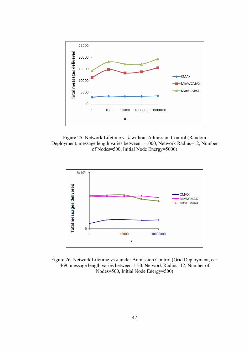
The effect of admission control can be observed by comparing the results sketched
in Figures 24, 25, 26 and 27. While in random deployment rejection of large
messages (where energy use becomes greater than the threshold, σ) degrades
performance, grid deployment is not affected by admission control. This seems a
bit counterintuitive at first, but the explanation is that one is able to “fit in” many
small messages when larger messages would no longer be routed. We conclude
that while admission control is necessary to achieve a good competitive ratio as
observed in [2] , it is not a good idea for network capacity on average.
Figure 22. Network Lifetime vs λ (Random Deployment, message length is constant, Network Radius=12, Number of Nodes=500, Initial Node Energy=500)

41
Figure 23. Network Lifetime vs λ (Grid Deployment, message length is constant, Network Radius=12, Number of Nodes=500, Initial Node Energy=500)
Figure 24. Network Lifetime vs λ under Admission Control (Random Deployment, σ = 6205, message length varies between 1-1000, Network Radius=12, Number of
Nodes=500, Initial Node Energy=5000)
42
Figure 25. Network Lifetime vs λ without Admission Control (Random Deployment, message length varies between 1-1000, Network Radius=12, Number
of Nodes=500, Initial Node Energy=5000)
Figure 26. Network Lifetime vs λ under Admission Control (Grid Deployment, σ = 469, message length varies between 1-50, Network Radius=12, Number of
Nodes=500, Initial Node Energy=500)

43
Figure 27. Network Lifetime vs λ without Admission Control (Grid Deployment, message length varies between 1-50, Network Radius=12, Number of Nodes=500,
Initial Node Energy=500)
3.4.5. Performance Comparison of Different Network Lifetime Definitions
We made the definitions of network lifetime and network capacity in Chapter I. To
emphasize it once more, maximum number of messages that can be delivered to
the sink until none of the paths are able to route a message defines network
capacity. Since we cannot claim to reach network capacity by running the
algorithm, this implies simply network lifetime definition in our simulations. (We
call it Network Lifetime I). As a second definition for lifetime, we also use
maximum number of messages that can be delivered to the sink until the first
failure of a message in the network (Network Lifetime II).
Although what we are really interested is an approximation to the network capaciy,
we would like to show the performance difference when the definition, Network
Lifetime II is considered as well. For random network topology, Figure 28 shows
expected results. For all algorithms, when Network Lifetime I is aimed,
performance is better. Furthermore, for grid topology, results are impressive
(Figure 29) since network with grid topology shows the same performance even if
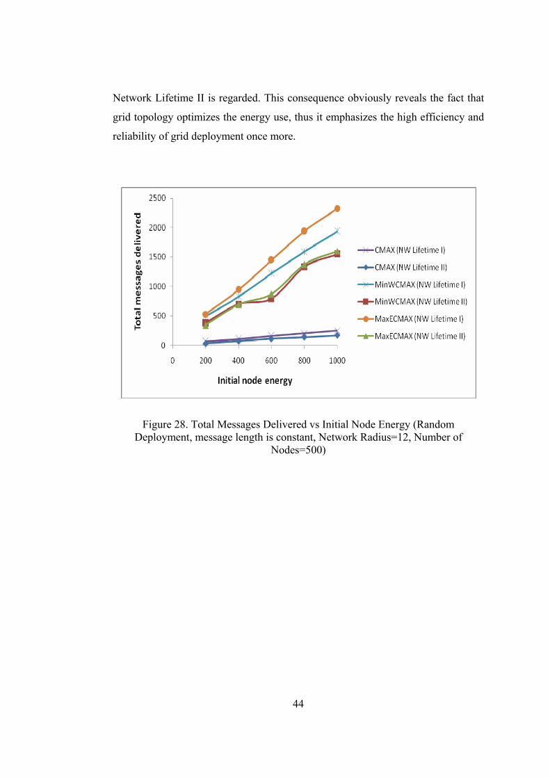
44
Network Lifetime II is regarded. This consequence obviously reveals the fact that
grid topology optimizes the energy use, thus it emphasizes the high efficiency and
reliability of grid deployment once more.
Figure 28. Total Messages Delivered vs Initial Node Energy (Random Deployment, message length is constant, Network Radius=12, Number of
Nodes=500)

45
Figure 29. Total Messages Delivered vs Initial Node Energy (Grid Deployment, message length is constant, Network Radius=12, Number of Nodes=500)
3.4.6. Scalability of Algorithms
In order to evaluate the scalability of our algorithm, we observe the effect of
network size while we keep the network density unity. We used the following
network sizes in simulations (Note that number of nodes is selected such that
average number of nodes in unit area is kept 1.) :
• Network Radius = 6, Number of Nodes = 113
(Network Area / # of Nodes = 1.00086)
• Network Radius = 12, Number of Nodes = 452
(Network Area / # of Nodes =1.00086)
• Network Radius = 18, Number of Nodes = 1018
(Network Area / # of Nodes = 0.99988)
We can see that our algorithm is completely scalable when the network is deployed
in grid topology (Figure 30). However, in random network topology, although
there is not a remarkable performance change, we observe that network lifetime
gets worse at the network of R = 18 and N = 1018 (Figure 31).

46
Figure 30. Comparison of Network Lifetime for Different Network Sizes where network radius R takes the values R=6,12,18 and number of nodes per unit
network area is 1 (Grid Deployment, MaxECMAX Algorithm)
Figure 31. Comparison of Network Lifetime for Different Network Sizes where network radius R takes the values R=6,12,18 and number of nodes per unit
network area n takes the values n=1.00086,1.00086,0.99988 respectively (Random Deployment, MaxECMAX Algorithm)

47
CHAPTER IV
IMPLEMENTATION ISSUES
4.1. Update of Residual Energy Information
All simulations have been performed based on the assumption that we have precise
knowledge of residual energy of any node at any time instant within network
lifetime. In reality, obviously the scenario will be different. There are two
implementation scenarios that we propose (Sections 4.1.1. and 4.1.2.) in order to
enable nodes to have knowledge about residual energies of their neighbors.
4.1.1. First Scenario (No Precise Knowledge)
In this scenario, to know the instantaneous energies of nodes, there will be no extra
energy usage such as a node’s broadcasting its residual energy. Here, unless a node
has previously forwarded a package to its neighbor, it will assume that its neighbor
has the initial energy Ei as if this neighbor has not sent any packages yet. If there
was an old event where the node used again the same neighbor to transfer data, the
latest residual energy information of the neighbor inherited from this old event is
used. Thus, a node updates its knowledge of a neighbor only when it sends the
package to this neighbor.
Advantages of first scenario: There is remarkable energy saving in this scenario
regarding the loss to keep up-to-date knowledge of residual energy by broadcasts.
It is also advantageous in terms of prevention of interferences as a result of extra
communications.

48
Disadvantages of first scenario: Since no precise knowledge of residual energy is
possible in this scenario, there will certainly be some wrong decisions. This means
that in some cases the most efficient and energy saving path will not be selected.
Thus, network lifetime will unavoidably decrease compared to the ideal case with
precise knowledge. On the other hand, to enable a node to update the residual
energy knowledge of its neighbor at a delivery, somehow a communication will be
needed between them or a reasonable assumption can be regarded.
4.1.2. Second Scenario (Precise Knowledge)
In this scenario, whenever a node forwards a package, it will broadcast its updated
energy to its neighbors. In this way, fresh and hence accurate residual energy
knowledge of neighbors will be guaranteed for any node in the network.
Advantages of second scenario: It will always enable use of accurate information,
i.e., precise knowledge at nodes. Therefore, we can be comfortable that really the
most efficient path will be selected for delivery.
Disadvantages of second scenario: It will bring a drawback of extra energy loss
due to the update broadcasts. However, this energy loss will be small compared to
real message delivery. Second, extra communication will bring interferences and
result in a MAC layer problem but this can be easily handled by TDMA structure.
As both of the scenarios have disadvantages as well as advantages it can be
reasonable to follow an approach in between. In addition to the knowledge updates
defined in first scenario, some periodical (but not so often) broadcasts may help to
have almost accurate knowledge of instantaneous energies.

49
4.2. Node with Maximum Energy
As a simplest solution when a node receives a message, it can broadcast that it has
data with length l and type X (We assume that all possible data types are well
defined and known by all sensors in network.).
The broadcast will enable both the neighbor with the maximum state energy to get
ready for message transmission and other neighbors with the same data to know
that message has already been broadcasted by another node so that it can silently
be dropped. In this implementation there are three main drawbacks:
1. It is difficult to define the data with certain attribute-value pairs. A good
solution to describe the data can be using a kind of hash algorithm to produce
fingerprints of the data as a description of it. Hence, hash information of the
data (assume that all nodes will be capable of computing the unique hash
information using the same hash function) can be used instead or alternatively,
a sequence with certain number of bits from the beginning and/or end of the
message can be used for comparison.
2. As the node will broadcast the data information only to its neighbors,
inevitably there will be more than 1 delivery for the same type of message if
there are also nodes apart from neighbors with the same data. To prevent this,
further but small complexity could be inserted to the implementation: We can
easily say that for almost all cases there will be common neighbors among
nodes. First, when the information of a specific message m is broadcast by
node i, all neighbors of i will know it is guaranteed that m will be sent to the
sink by the selected maximum-energy node. Later if somehow the information
of m is also broadcast by another node j (j is not a neighbor of i) we can easily
assume that there will be at least 1 node from i’s neighbors that can quickly
warn node j that m has already been decided to be delivered. Hence after this
WARN message, j will secondly broadcast a CANCEL message to its

50
neighbors so that all can comfortably drop m to prevent re-deliveries. In this
approach, WARN and CANCEL messages will be of very short size so they
will not cause considerable energy loss.
3. It is also difficult how a sensor and others will know that it has the highest
residual energy. As a practical solution, this condition can be desisted from and
the first node making the broadcast of the data can send instead. It will not be
guaranteed to deliver m from the node with highest state energy. However, in
any case, clearly it will be more efficient than double or more transmissions.
4.3. Minimum Weight Path Calculation
At current simulations, by means of Dijkstra’s Algorithm, it is guaranteed to select
the path with minimum total weight among all possible paths [12]. However, in
practical case it will be difficult to apply precisely Dijkstra because comparison of
computed paths will be needed in order to decide the minimum one and eventually
knowledge of those paths will be required by nodes. At this point, a minimum
weight decision at a single hop may help. By this approach, the source node will
select the minimum weight link among all links to its neighbors and send from this
link and the process will continue until the destination node is reached.

51
CHAPTER V
CONCLUSION
We started by arguing that neither the class of routing algorithms that are based on
energy-efficient topologies, nor the class of algorithms that are data-centric can
alone achieve network capacity in an energy-constrained wireless network. Using
the CMAX algorithm by Kar et al. as a benchmark, we proposed a proof-of-
concept routing algorithm that combines the approaches of both classes, under
highly idealized assumptions, such as the availability of centralized decision-
making. The algorithm aggregates data, and sends them along minimum-weight
paths, where weight is a function of both residual node energy and transmission
energy on the links along the path. We showed that this causal (online) routing
algorithm achieves the same competitive ratio as CMAX with respect to a
potentially much higher network capacity. We have found that network capacity is
maximized under a grid-type node deployment. With random node deployment,
capacity is lower (network lifetime is shorter.)
This study can be regarded as preliminary work for the development of an energy-
optimal online routing algorithm. A number of practical issues, that is widely
discussed in this thesis, need to be addressed in future work. An important one is
the following: It is impractical to assume that every node knows current states
(residual energy) of all other nodes. In practice, there is energy cost to obtain this
state information; thus, there is a tradeoff between the energy used to gather state
information and the energy saved by using accurate information in routing
decisions. We believe a good design will need to find good operating points in this
tradeoff.

52
CHAPTER VI
FURTHER DIRECTIONS
This thesis involves an overview of advantages and disadvantages of data-centric
and energy-centric WSN routing algorithms. Beyond the analysis of existing
algorithms, it proposes how to combine the good features of them to design an
energy-constrained online algorithm, that is close to the network capacity.
Furthermore, it compares two different types of network topologies (random
network topology, grid network topology) with the conclusion of better
performance of grid topology.
Considering these main results, our study will provide a background for a number
of future directions.
Rather than using an existing algorithm as a benchmark, a completely new routing
algorithm can be proposed addressing all the important issues referred in this
thesis. The results and experiences gained from the simulations of MinWCMAX
and MaxECMAX can be used. More investigation should be made in order to
define an optimal cost function and eij. In addition to the exact definition of
shortest path calculation, a clear procedure for data aggregation should also be
specified so that implementation issues can be handled better. Here, it is very
critical to make a good tradeoff between the energy consumptions for the updates
of state information and the energy savings by using accurate information in
routing decisions.
Besides design of the algorithm, setting up a solid base for the algorithm itself is
crucial. From this point of view, we could propose the following analytical
directions:

53
• Theoretically justified, a good lower bound on the performance ratio
can be studied without a necessity for admission control. It would
really be an advance if a bound could be found without rejecting
any of the messages in the network, that is much more realistic.
• Investigation of an upper bound on the performance ratio would
also help us have an idea how much the algorithm can get closer to
the optimal network capacity, i.e., how much the network
performance can be improved.
There are many implementation issues that need to be addressed so that a
practically useable algorithm can be proposed to the WSN community. The
implementation discussion in Chapter IV can be starting point to handle such
practical problems.
This thesis studied the model of a circular network where events are generated
around the network and there is a single sink at the center, at future work design of
the algorithm should enable more than one destination node as well as a variety of
event generation locations.

54
REFERENCES
[1] Chee-Yee Chong, Srikanta P. Kumar, Sensor Networks: Evolution,
Opportunities, and Challenges, Proceedings of the IEEE, Vol. 91, No. 8,
August 2003, pp. 1247-1256.
[2] Koushik Kar, Murali Kodialam, T. V. Lakshman, Leandros Tassiulas,
Routing for Network Capacity Maximization in Energy-constrained Ad-hoc
Networks, Infocom 2003 Twenty-Second Annual Joint Conference of the IEEE
Computer and Communications Societies, pp. 673-681.
[3] J-H. Chang, L. Tassiulas, Energy conserving routing in wireless ad-hoc
networks, Proc. of Infocom 2000, March 2000, pp. 22-31.
[4] Jae-Hwan Chang, Tassiulas L., Maximum lifetime routing in wireless
sensor networks, IEEE/ACM Transactions on Networking, August 2004, pp.
609-619.
[5] C. Intanagonwiwat, R. Govindan, D. Estrin, Directed diffusion: a scalable
and robust communication paradigm for sensor networks, Proceedings of the
ACM Mobi-Com’00, Boston, MA, 2000, pp. 56–67.
[6] Lawrence A. Bush, Christopher D. Carothers and Boleslaw K. Szymanski,
Algorithm for Optimizing Energy Use and Path Resilience in Sensor Networks,
Proceedings of the Second European Workshop on Wireless Sensor Networks,
2005, pp. 391-396.
[7] Balakrishnan M., Johnson E.E., Fuzzy diffusion for distributed sensor
networks, IEEE Military Communications Conference, Milcom, 2005, pp.
3023-3028.
[8] W.R. Heinzelman, J. Kulik, H. Balakrishnan, Adaptive protocols for
information dissemination in wireless sensor networks, Proceedings of the
ACM MobiCom’99, 1999, pp. 174–185.
[9] Q. Li, J. Aslam, and D. Rus, Online power-aware routing in wireless ad hoc
networks, IEEE/ACM Int. Conf. Mobile Computing and Networking
(MobiCom 2001), July 2001, pp. 97-107.
55
[10] S. Singh, M.Woo, and C. S. Raghavendra, Power-aware routing in mobile
ad hoc networks, Proc. IEEE/ACM Int. Conf. Mobile Computing and
Networking, October 1998, pp. 181–190.
[11] V. D. Park and M. S. Corson, A highly distributed routing algorithm for
mobile wireless networks, Proc. IEEE INFOCOM, 1997, pp. 1405–1413.
[12] E.W Dijkstra, A Note on Two Problems in Connexion with Graphs,
Numerische Mathematik, Vol. 1, 1959, pp. 269-271.
[13] Muruganathan S.D., Ma D.C.F., Bhasin R.I., Fapojuwo A.O., A centralized
energy-efficient routing protocol for wireless sensor networks, IEEE
Communications Magazine, Vol. 43, March 2005, pp. S8-13.
[14] Dagher J.C., Marcellin M.W., Neifield M.A., A Theory for Maximizing the
Lifetime of Sensor Networks, Communications, IEEE Transactions on, Vol.
55, Feb 2007, pp. 323-332.
[15] Luo H., Liu Y., Das S. K., Routing Correlated Data with Fusion Cost in
Wireless Sensor Networks, Mobile Computing , IEEE Transactions on, Vol. 5,
Nov 2006, pp. 1620-1632.
[16] A. Cerpa et al., “Habitat monitoring: Application driver for wireless
communications technology,” 2001 ACM SIGCOMM Workshop on Data
Communications in Latin America and the Caribbean, Costa Rica, April 2001.
[17] G.J. Pottie, W.J. Kaiser, “Wireless Integrated Network Sensors,”
Communications of the ACM, vol. 43, no. 5, pp. 551-8, May 2000.
[18] J. Warrior, “Smart Sensor Networks of the Future,” Sensors Magazine,
March 1997.
[19] I.F. Akyildiz, W. Su, Y. Sankarasubramaniam, E. Cayirci, Wireless sensor
networks: a survey, IEEE Computer Networks, 2002, pp. 393-422.
[20] Krishnamachari B., Estrin D., Wicker S., Modelling Data-Centric Routing
in Wireless Sensor Networks, IEEE INFOCOM 2002.
[21] V. Rodoplu and T.H. Ming, "Minimum energy mobile wireless networks,"
IEEE Journal of Selected Areas in Communications, Vol. 17, No. 8, pp. 1333-
1344, 1999.
56
[22] L. Li and J. Y Halpern, “Minimum energy mobile wireless networks
revisited,” in the Proceedings of IEEE International Conference on
Communications (ICC’01), Helsinki, Finland, June 2001.
[23] B. Krishnamachari, D. Estrin, and S. Wicker, “Impact of Data Aggregation
in Wireless Sensor Networks,” Proc. 22nd Int’l Conf. Distributed Computing
Systems, pp. 575-578, July 2002.
[24] A. Scaglione and S.D. Servetto, “On the Interdependence of Routing and
Data Compression in Multi-Hop Sensor Networks,” Proc. ACM MobiCom,
Sept. 2002.
[25] W.R. Heinzelman, A. Chandrakasan, and H. Balakrishnan, Energy-
Efficient Communication Protocol for Wireless Microsensor Networks,” Proc.
33rd Ann. Hawaii Int’l Conf. System Sciences, Jan. 2000.
[26] S. Lindsey and C. S. Raghavendra, "PEGASIS: Power Efficient GAthering
in Sensor Information Systems," in the Proceedings of the IEEE Aerospace
Conference, Big Sky, Montana, March 2002.
[27] M. Younis and K. Akkaya, A Survey on Routing Protocols for Wireless
Sensor Networks, Elsevier Ad Hoc Network Journal 2005, Vol. 3/3 pp. 325-
349.
[28] Schurgers C., Srivastava M.B., Energy Efficient Routing in Wireless
Sensor Networks, MILCOM'01, Vienna, VA, pp. 357-361, October 28-31,
2001.
[29] Trong Thua HUYNH Choong Seon Hong, "An Energy*Delay Efficient
Multi-Hop Routing Scheme for Wireless Sensor Networks",IEICE
TRANSACTIONS on Information and Systems, Vol.E89-D No.5, pp.1654-
1661, May 2006.
[30] Hassanein, H.; Jing Luo; Reliable Energy Aware Routing in Wireless
Sensor Networks, Dependability and Security in Sensor Networks and
Systems, DSSNS 2006. Second IEEE Workshop, April 2006 pp. 54 – 64.
[31] C. Intanagonwiwat, D. Estrin, R. Govindan, and J. Heidemann, “Impact of
Network Density on Data Aggregation in Wireless Sensor Networks,” Proc.
22nd Int’l Conf. Distributed Computing Systems, July 2002.

57
[32] W. Zhang and G. Cao, “Optimizing Tree Reconfiguration for Mobile
Target Tracking in Sensor Networks,” Proc. IEEE INFOCOM, Mar. 2004.
[33] A. Goel and D. Estrin, “Simultaneous Optimization for Concave Costs:
Single Sink Aggregation or Single Source Buy-at-Bulk,” Proc. ACM-SIAM
Symp. Discrete Algorithms, Jan. 2003.
[34] R. Cristescu, B. Beferull-Lozano, and M. Vetterli, “On Network Correlated
Data Gathering,” Proc. IEEE INFOCOM, Mar. 2004.
[35] P.V. Rickenbach and R. Wattenhofer, “Gathering Correlated Data in
Sensor Networks,” Proc. ACM Workshop Foundations of Mobile Computing,
Oct. 2004.
[36] Cheng C., Energy Efficient Routing for Clustered Wireless Sensors
Network, Industrial Electronics Society, 2003. IECON '03. The 29th Annual
Conference of the IEEE, Vol. 2, pp.1437 – 1440.
[37] Lukachan G., Labrador M.A., Moreno W., Scalable and Energy-efficient
Routing for Large-scale Wireless Sensor Networks, Proceedings of the 6th
International Caribbean Conference on Devices, Circuits and Systems, Mexico,
Apr. 2006, pp. 267-272.
[38] Al-Karaki, J.N.; Al-Mashagbeh, G.A.; Energy-Centric Routing in Wireless
Sensor Networks, Computers and Communications, 2006. ISCC '06.
Proceedings. 11th IEEE Symposium pp. 948 – 954.

58
APPENDIX A
SIMULATION SOURCE CODES
//Here, we provide the body of main program, the complete source code including //all the functions called in the main program will be available in a CD attached to //this thesis.
//This function clears events of each node of the network
void clear_Events_InNetwork()
{
Sensor* sensortemp = sensorhead->next;
while(sensortemp != sensortail)
{
sensortemp->event_ID = -1;
sensortemp = sensortemp->next;
}
}
//This function assigns event with the given id to the node if the event is in the range of the node.
void fill_Msg_Sensor(int id)
{
Sensor* sensortemp = sensorhead->next;
Event* temp_event = event_Head->next; //
while(sensortemp!=sensortail)
{
sensortemp->event_ID = -1;
sensortemp->has_sended = -1;
sensortemp = sensortemp->next;
}
while(temp_event!=event_Tail)

59
{
if(temp_event->id == id)
break;
temp_event = temp_event->next;
}
if(!temp_event->event_sent && temp_event != event_Tail)
{
sensortemp = sensorhead->next;
while(sensortemp!=sensortail)
{
double dist = (temp_event->pos_X - sensortemp->Pos_X)*(temp_event->pos_X - sensortemp->Pos_X)
+(temp_event->pos_Y - sensortemp->Pos_Y)*(temp_event->pos_Y - sensortemp->Pos_Y);
dist = pow(dist,1.0/2.0);
if(dist < temp_event->radius)
sensortemp->event_ID = temp_event->id;
sensortemp = sensortemp->next;
}
}
}
//This function executes the CMAX algorithm for a given event.
void Pure_Tassiulas_Main(Event* temp_event)
{
Sensor* sensortemp = sensorhead->next;
bool stop_continue = true;
sensortemp = sensorhead->next;
while(sensortemp!=sensortail)
{

60
if((sensortemp->event_ID != -1) && (sensortemp->event_ID == temp_event->id)&& (sensortemp->has_sended == -1) )
{
if(temp_event != NULL)
{
message_Length = temp_event->message_Lenght;
Target_sensor = sensorhead->next;
Source_sensor = sensortemp;
stop_continue = Dijkstra(Source_sensor, Target_sensor,1/*pure tassiulas Func ID*/, temp_event); // We have already set 'sensorhead->next' sensor at (0,0) point
if(!stop_continue) break;
}
}
sensortemp = sensortemp->next;
}
sensortemp = sensorhead->next;
while(sensortemp!=sensortail)
{
sensortemp->has_sended = -1;
sensortemp = sensortemp->next;
}
}
//This function executes CMAX algorithm after filling events
//which are in the range of the nodes, it calls Pure_Tassiulas_Main function.
void Pure_Tassiulas()
{
Event* temp_event = event_Head->next;
int tot_event = num_of_events;
while(tot_event > 0)

61
{
int re = rand();
re %=num_of_events;
temp_event = event_Head->next;
for(int i=0;i<=re;i++)
{
if(temp_event != event_Tail && !temp_event->event_sent && temp_event->id == re+1)
{
fill_Msg_Sensor(temp_event->id);
Pure_Tassiulas_Main(temp_event);
tot_event--;
break;
}
temp_event = temp_event->next;
}
if(no_PATH_FOUND > 20)
{
no_PATH_FOUND=0;
break;
}
}
temp_event = event_Head->next;
int dummy = 0;
while(temp_event!=event_Tail)
{
if(temp_event->event_sent)
{
cout<<"Event "<<temp_event->id<<" ";
temp_event->event_sent = false;
dummy++;
}

62
temp_event = temp_event->next;
}
if(dummy)
cout<<"have been sent, TOTAL: "<<dummy<<" events."<<endl;
}
//This function takes the user inputs and executes the specified functions and algorithms.
void Method_Decision(int *count)
{
int method;
cout<<" To specify source & destination Nodes from command line, press '0'"<<endl;
cout<<" To send messages from the event list using Pure Tassiulas Algorithm, press '1'"<<endl;
cout<<" To send messages from the event list selecting the min of all shortest paths calculated(Theoretical Proposal), press '2'"<<endl;
cout<<" To send messages from the event list selecting the node with max. Energy(Practical Proposal), press '3'"<<endl;
cin>>method;
if(method == 0)
{
take_Target_Source();
Dijkstra(Source_sensor, Target_sensor,-1, NULL);
}
else if(method == 1)
{
//fill_Msg_Sensor();
Pure_Tassiulas();
*count = *count + 1;
cout<<"\nTASS algorithm has run for "<<(*count)<<" times\n";
print_Min_Path();
}
else if(method == 2)
{

63
//readEventList(); // read Event.txt.
//fill_Msg_Sensor(); // fill event id to the node which recognise an event.
evaluate_Graph();
count_Affected_Sensors();
print_Min_Path();
}
else if(method == 3)
{
//readEventList(); // read Event.txt.
//fill_Msg_Sensor(); // fill event id to the node which recognise an event.
select_Max_State_Energy();
count_Affected_Sensors();
print_Min_Path();
}
cout<<"Average Number of Hops= "<<(float)total_Nodes_onPaths/(float)found_Path_Number<<endl;
cout<<"Average of 1/Hops= "<<(float)TotalOneOverPath/(float)found_Path_Number<<endl;
found_Path_Number = 0;
total_Nodes_onPaths = 0;
TotalOneOverPath = 0.0;
}
//It is the main function of all the program and
//takes the user inputs then executes the specified functions and algorithms.
int main()
{
int Tass_Count = 0;
sensorhead = new struct Sensor; //while starting the program taking space to the head & tail pointers...
sensortail = new struct Sensor;
sensorhead->next = sensortail; sensorhead->prev = NULL;
sensortail->prev = sensorhead; sensortail->next = NULL;

64
priorty_Head = new struct min_Priority ; //while starting the program taking space to the head & tail pointers...
priorty_Tail = new struct min_Priority ;
priorty_Head->next = priorty_Tail;
priorty_Tail->prev = priorty_Head;
event_Head = new struct Event;
//while starting the program taking space to the head & tail pointers...
event_Tail = new struct Event;
event_Head->next = event_Tail;
event_Tail->prev = event_Head;
Eij_Head = new struct min_Eij;
//while starting the program taking space to the head & tail pointers...
Eij_Tail = new struct min_Eij;
Eij_Head->next = Eij_Tail;
Eij_Tail->prev = Eij_Head;
char key;
take_Inputs();
calculate_Lambda();
while(1)
{
cout<<"\n\n1) For sending new messages press 'S'/'s'"<<endl;
cout<<"2) For loading graph from beginning of the configuration press 'L'/'l'"<<endl;
cout<<"3) For List Border Edges Press 'B'/'b'"<<endl;
cout<<"4) For reading 'event list' press 'e/E'"<<endl;
cout<<"5) For exit press q/Q\n"<<endl;
cin>>key;
if(key == 'Q' || key == 'q')
break;
65
else if(key == 'l' || key == 'L')
{
reLoad_Graph();
construct_GraphFromText();
}
else if(key == 'B' || key == 'b')
{
listBorderEdges();
}
else if(key == 's' || key == 'S')
{
Method_Decision(&Tass_Count);
}
else if(key == 'e' || key == 'E')
{
cout<<"To create a new event List press C/c"<<endl;
char de;
cin>>de;
if(de=='C' || de=='c')
{
//create new event list
int total_events;
float evn_radius;
cout<<"Now enter the total number of events"<<endl;
cin>>total_events;
while(total_events<1)
{
cout<<"The given event number must be greater than '0'"<<endl;
cin>>total_events;
}
cout<<"Enter the radius of the event list"<<endl;
scanf("%f", &evn_radius);

66
while(evn_radius <= 0.0)
{
cout<<"The given event radius must be greater than '0.0'"<<endl;
scanf("%f", &evn_radius);
}
createEvent(evn_radius, total_events);
}
delete_List();
readEventList();
}
else
cout<<"The given character is not one of the aboves!!!"<<endl;
}
cout<<"Total message delivered: "<<Total_Message_Length<<endl;
//calculate_Edge_Weights();
if(error)
return -1;
system("pause");
return 0;
}