Exhibit 28

i

LNG and Renewable Power

Risk and Opportunity in a Changing World

PREPARED BY

Jurgen Weiss, PhD

Steven Levine

Yingxia Yang, PhD

Anul Thapa

January 15, 2016

All results and any errors are the responsibility of the authors and do not represent the opinion

of The Brattle Group, Inc. or its clients.

Acknowledgement: We acknowledge the valuable contributions of many individuals to this

report and to the underlying analysis, including members of The Brattle Group for peer review.

Copyright © 2016 The Brattle Group, Inc.

i | brattle.com

Table of Contents

Executive Summary .............................................................................................................................. ii

I. Introduction ................................................................................................................................. 1

II. The Cost of LNG Infrastructure .................................................................................................. 5

III. The Cost of Renewable Power Generation .............................................................................. 11

IV. Comparing the Cost of LNG and Renewables.......................................................................... 16

V. Discussion .................................................................................................................................. 25

VI. Electric Market Uncertainties and Gas Market Competition: Implications for LNG Markets ....................................................................................................................................... 30

VII. Conclusions ................................................................................................................................ 34

ii | brattle.com

Executive Summary

Two important trends are transforming the energy industry across the globe. The production of

relatively low-cost unconventional sources of natural gas—primarily in the United States and

Canada, but potentially also in other parts of the world—has led to much heightened attention to

the possibility of increased use of Liquefied Natural Gas (“LNG”) in world markets and a large

number of proposed LNG export projects in North America. Several LNG export projects are

under construction in North America (and will begin exporting in the next few years), and many

more are proposed with the hope of being part of a “second wave” of LNG projects to begin

service in the post-2020 time frame. At the same time, both technological progress and concerns

about climate change risks are stimulating the development and deployment of various types of

renewable energy sources around the world.

While the natural gas industry has traditionally viewed LNG as a substitute for oil in many

markets, this paper explores whether the evolution of renewable energy sources suggests that

LNG may be competing less with oil and more with renewable energy sources in markets outside

of North America in the coming years. Such competition is evident in electricity generation

markets as natural gas combined-cycle units and renewable energy sources compete to serve

future electricity demand. Competition between natural gas and efficient electric heating (using

heat pumps, for example) is less prominent, but emerging in some countries (e.g., Germany).

Thus, there are important and intensifying linkages between global natural gas and electricity

markets that will impact developments in renewables markets and have feedback effects into the

natural gas market.

This emphasis on LNG development takes place against a backdrop of several important market

dynamics, including the recent collapse in world oil prices, a slow-down in China’s economy and

its demand for natural gas, the commissioning of new LNG export projects in Australia, and a

reduced need for natural gas in Japan due to the re-start of some of the country’s nuclear power

plants. As a result of these factors, Asian LNG prices, which had risen to $15/MMBtu (or more)

in recent years, have now collapsed to roughly $6-$7/MMBtu, and the significant price

differential between world oil prices and North American natural gas prices (that gave rise to the

North American LNG projects now in development) has now declined dramatically. The

deterioration of this price differential is bad news for both the LNG export projects in

development (but not under construction) in North America and the energy companies that

iii | brattle.com

signed up for long-term LNG export capacity from the new North American export projects (that

are under construction and one of which will begin service in early 2016). These market

suppliers need LNG delivered prices in Asia to be in the $10-$11 range in order to be profitable.

With several more LNG export projects coming online in the 2015-2020 period and an

expectation of continued low oil prices, global LNG markets are likely to be oversupplied for the

next several years and the low LNG prices now observed seem likely to persist for some time.

The fate of many of the proposed North American LNG export projects is increasingly uncertain

in the new price environment (and some LNG export projects have already been delayed).

Thus, two important questions facing global LNG markets today are how quickly LNG supplies

associated with the new LNG projects coming online over the next few years will be absorbed,

and at what point in the future there might be a rebound in global LNG prices such that new

LNG export terminals (beyond the terminals now under construction) are needed. The LNG

export developers in North America (as well as buyers of LNG from the projects now under

construction) are hoping that the worldwide LNG supply glut is temporary and that market

conditions in the post-2020 time frame will improve.

The analysis in our paper suggests that market participants should be very cautious in thinking

that the LNG supply glut is necessarily a temporary problem, because another important

dynamic in world energy markets is the declining cost of renewable power and the prospect of

increased penetration of renewables in the global power generation mix and thus competing

with LNG as a “fuel source” for power generation. In fact, in some regions such as Germany and

California, where renewable penetration has been high, gas demand growth has already been

stunted by the penetration of renewables in the generation mix (causing a reduction in gas

demand growth for power generation).

There is a real possibility of a significant shift towards more renewable power generation in some

of the key Asian markets targeted by the LNG industry. While the current shares of wind, solar,

and gas in China are each less than 5% of China’s total electricity generation, all three sources of

electricity generation are projected to increase substantially over the next 25 years as the share of

coal generation as a percentage of total generation is projected to decline significantly from

iv | brattle.com

around 75% today to roughly 50% by 2040.1 Gas, wind, and solar (as well as nuclear) will

therefore all be competing to serve China’s growing electricity needs. The relative costs of LNG

and renewables discussed in this paper will likely be a significant factor determining which

technologies achieve the highest penetration levels. Of course, the uncertainties regarding the

costs of both renewables and delivered LNG over the coming decades remain significant and

other factors not discussed in this paper will influence China’s future electricity generation mix.

Nonetheless, the expectation of declining costs of renewables (discussed in this paper) relative to

LNG is noteworthy and creates the possibility of a potential shift towards even more renewable

generation than is currently forecast in key Asian markets.

Since many LNG forecasts suggesting that the LNG supply glut is temporary rely on the

assumption that natural gas demand from China and other countries in Asia will more than

double in the next 20 years (in part due to gas demand in the power sector), these forecasts

should be seen as highly uncertain given the potential for a significant shift towards more

renewable power in China and throughout Asia that could limit the growth in gas demand and

the need for LNG. Likewise, in Europe, despite the fact that declines in domestic natural gas

production (as well as the perpetual desire to diversify away from Russian-sourced natural gas)

are leading many to look at LNG as a potential alternative, the on-going shift towards more

renewables may reduce the incentive to import significantly larger amounts of LNG.

LNG infrastructure is very capital intensive across the entire LNG supply chain. As a result of

the billions of dollars of fixed costs, LNG projects and associated financing arrangements usually

require long-term contractual arrangements for the necessary infrastructure. These contractual

arrangements allow the developers of the LNG infrastructure to pass the risk of their projects on

to their counterparties. For example, the developers of LNG export projects may sell their export

capacity to large energy companies (such as BP, BG, Total) who then assume the risk for selling

LNG to overseas customers. In other cases, the developers may contract directly with overseas

1 See, for example, World Energy Outlook 2015, p. 634, which forecasts the share of gas-fired

generation (as a percent of total electricity generation) in the New Policies Scenario to grow from 2% in 2013 to 8% in 2040. WEO forecasts the share of wind generation to grow from 3% to 10%, and the share of solar PV to grow from 0 to 3% over this time period. Growth in generation from gas, wind, and solar PV over this time period is forecast to be 788 TWh, 886 TWh, and 353 TWh, respectively. Growth in installed capacity from gas, wind, and solar PV over this time period is forecast to be 160 GW, 321 GW, and 258 GW, respectively.

v | brattle.com

end-users. In either case, the risks can be substantial, especially because how much gas will be

needed overseas is uncertain, e.g., for gas-fired electricity generation purposes future needs may

not be known with any meaningful precision at the time long-term contracts are signed. LNG

project developers will also not be completely shielded from risk for several reasons: the capital

recovery period may extend beyond the term of their initial long-term contracts, the capacity of

a given LNG project may not be fully subscribed, they will be subject to the ongoing

creditworthiness of their counterparties, and they may face demands for contract price

adjustments as market conditions and the competitive LNG landscape changes. Thus, market

participants along the LNG supply chain need to understand how the development of renewable

resources in overseas markets could impact the need for LNG imports in those markets.

Ultimately, investments in North American LNG terminals2 require that the prices paid for LNG

in overseas markets are greater than or equal to the price of U.S. natural gas supplies (e.g., at

Henry Hub) plus the cost of all infrastructure necessary to liquefy and deliver LNG to overseas

markets (including a fair rate of return on that infrastructure). If the cost of renewable

generation is low enough overseas (i.e., below the cost of new gas-fired generation burning LNG

from North America), it could dampen the attractiveness of North American-sourced LNG as a

fuel for electric generation and the willingness of market participants to continue to contract for

LNG export infrastructure.

We find that the competition between renewable power and gas-fired generation using LNG

delivered from North America is increasing in overseas markets. Our conclusion is based on an

analysis of the costs of developing new gas-fired generation in Asian and European markets that

use LNG from North America as a fuel source compared to the costs of developing new

renewable generation in those markets. Our estimate of the delivered cost of LNG from North

America includes both the forecasted commodity cost of North American gas supplies (from the

U.S. Energy Information Administration) and the infrastructure costs of liquefaction, shipping,

and regasification necessary for North American gas to be consumed in Asian and European

markets.

2 While this paper specifically discusses the risks posed by the declining cost of renewable energy to

North American LNG developers and their customers, a similar dynamics between renewables and LNG could also broadly apply to other regions.

vi | brattle.com

The delivered cost of LNG is shown as the gray and blue shaded areas of the chart in Figure ES-1

below. To compare the delivered LNG cost to the cost of renewable generation, we calculate the

equivalent gas price (shown as lines) at which new gas-fired power generation would have the

same levelized cost as new renewable generation (assuming regional costs and at various assumed

capacity factors).3 As can be seen in Figure ES-1, in China this comparison suggests that wind

generation with a capacity factor of 25% (the yellow line in Figure ES-1) would already be

competitive with power generation using LNG delivered from North America at a delivered cost

to China of roughly $11/MMBtu (reflecting full recovery of LNG infrastructure costs and a U.S.

gas commodity cost of approximately $3.00/MMBtu). Moreover, our analysis shows a risk that

wind power in China with capacity factors as low as 20% may become competitive with

combined-cycle generation using North American LNG within the next 5 years (at which point

delivered LNG prices are forecast to exceed $13/MMBtu).

These are important findings, especially with respect to the many proposed LNG export projects

in North America (in the U.S. Gulf Coast, Alaska, and Canada) that are still in the early

development phase. The investment risk of these proposed LNG export projects is increasing

because there is a significant possibility that, over the 20 years of a typical LNG contract, power

production from renewable energy sources will become less costly than the LNG sales prices

needed to justify the upstream LNG investment cost (even without considering the value of

avoided greenhouse gas emissions).

While LNG looks more favorable when compared to stand-alone solar PV and wind in Germany,

which, due to its emphasis on renewable energy, we use as an example for potential LNG exports

to Europe, a mix (hybrid) of wind and solar and/or a strengthening carbon price could equally

lead to renewables becoming less expensive than combined-cycle generation using North

American LNG in the coming years, as shown in Figure ES-2.

3 First, we calculate the levelized cost of electricity (LCOE) for renewables in $/MWh using assumed

capital costs, fixed operations and maintenance (FOM) costs and renewable capacity factors. We then transform this LCOE in $/MWh into an equivalent gas price in $/MMBtu by calculating the natural gas price that makes the LCOE (in $/MWh) of a new combined cycle gas plant equal to the calculated LCOE for renewables in $/MWh (using assumed capital costs, FOM, VOM, and heat rate of a new gas-fired combined cycle power plant).

vii | brattle.com

Figure ES-1: Wind costs (in $/MMBtu) compared to the cost of New Gas-Fired Combined Cycle in China

Based on Forecast Delivered Cost of LNG from U.S. to China

Sources/Notes: World Energy Outlook 2013 for renewables cost assumptions (NPS Scenario). Delivered LNG cost breakdown from Figure 7 in main report.

Figure ES-2: The economics of a hybrid wind-solar plant and LNG-fueled power generation in Germany

with carbon emissions’ cost of $30/ton Based on Forecast Delivered Cost of LNG from U.S. to Europe

Sources/Notes: World Energy Outlook 2013 for renewables cost assumptions (NPS Scenario). Using forecast of delivered cost of U.S. LNG to Europe from Figure 8 in main report.

viii | brattle.com

Of course, this simple analysis does not account for all costs that affect the economic

attractiveness of using imported LNG or renewable power. For example, we exclude electricity

transmission and distribution infrastructure costs as well as other so-called “renewable

integration costs” from our analysis, even though they may be significant at higher levels of

renewable penetration and hence could make them less attractive compared to LNG. On the

other hand, carbon pricing could become important in LNG export markets other than Europe

and tip the scale further in favor of renewables. Also, the cost-overrun and delay risks associated

with the massive infrastructure investments needed to export LNG are potentially significant.

Developing a deeper understanding of the relationship between the cost of LNG-fueled gas-fired

and renewable power generation is therefore critically important in assessing the outlook for

both renewable power and the potential demand for LNG and associated infrastructure. The

competition between LNG-fueled gas-fired generation and renewable resources represents a risk

to participants in the LNG industry in that higher than expected renewables penetration could

reduce future natural gas demand growth (and LNG demand growth) in some of the key overseas

Pacific Asian markets. Of course, the reverse is also true: lower renewables penetration in

countries planning to develop substantial renewable resources could potentially lead to higher

than expected gas demand and LNG growth. While many other factors could impact the demand

for LNG in overseas markets (such as the future of nuclear generation, overall load and

population growth, potential competition from pipeline imports, etc.), this paper focuses on the

specific relationship between the cost of gas-fired generation using LNG and renewables.

The increasing competition between renewable power and gas-fired generation using LNG

should be considered carefully by participants in the global LNG markets. This competition

increases the uncertainty in global gas demand and the future LNG requirements in markets now

being targeted by North American LNG export developers. Both investors in LNG infrastructure

and buyers of LNG under long-term contracts will want to consider these risks before making

large and long-term commitments to buying or selling LNG.

1 | brattle.com

I. Introduction

The development of unconventional natural gas resources primarily in North America and the

relative abundance of natural gas in other parts of the world including Australia and the Middle

East have triggered a fundamental rethinking of the future global energy system and the role of

Liquefied Natural Gas (“LNG”). While these regions, and particularly the United States and

Canada, are hopeful for an energy future characterized by low energy costs as a result of these

abundant natural gas supplies, much of the rest of the world faces relatively higher natural gas

prices and pressures to move away from coal as a major source of energy, and has few low cost

alternatives.

Not surprisingly, the abundance of shale gas in North America, expectations that the cost of these

shale resources will remain relatively low, and corresponding expectations of relatively high

natural gas prices in much of the rest of the world have led to a wave of proposed large-scale

infrastructure projects designed to profit from the apparent arbitrage opportunities. These LNG

export projects will allow low-cost American natural gas to be transported and resold into

markets with high natural gas prices. North American LNG exports will therefore increase the

LNG export-related activity already strong in the Middle East and expanding in Australia.

At present, over 40 LNG export projects representing over 50 Bcf/d of export capacity (or roughly

70% of U.S. gas demand) are proposed in the United States, and over 20 projects representing

around 31-47 Bcf/d of capacity are proposed in Canada. As of the end of 2015, 10 LNG terminals

have received U.S. Department of Energy (“DOE”) approval to export approximately 14 Bcf/d of

LNG to non-Free Trade Agreement (“non-FTA”) countries, and five of these are now under

construction.4 Since LNG infrastructure is extremely capital intensive, its construction rationale

relies significantly on assumptions that gas prices in the North America will remain relatively

low and gas and oil prices (and gas demand) in the rest of the world will remain relatively high.

Such assumptions are typically justified based on a combination of factors, including expectations

4 The terminals under construction include Sabine Pass LNG (2.76 Bcf/d), Cameron LNG (1.7 Bcf/d),

Freeport LNG (1.8 Bcf/d), Cove Point LNG (0.82 Bcf/d), and Corpus Christi LNG (2.14 Bcf/d). See North American LNG Import / Export Terminal: Approved, FERC, as of October 20, 2015 available at:

http://www.ferc.gov/industries/gas/indus-act/lng/lng-approved.pdf.

2 | brattle.com

of the continued availability of low-cost U.S. shale supplies, growing demand for natural gas in

relatively fossil-resource-poor parts of the world, on-going gas-on-oil competition, and the

difficulty and/or high cost of opening up these markets to gas supplies other than through LNG

(i.e., through pipeline imports).

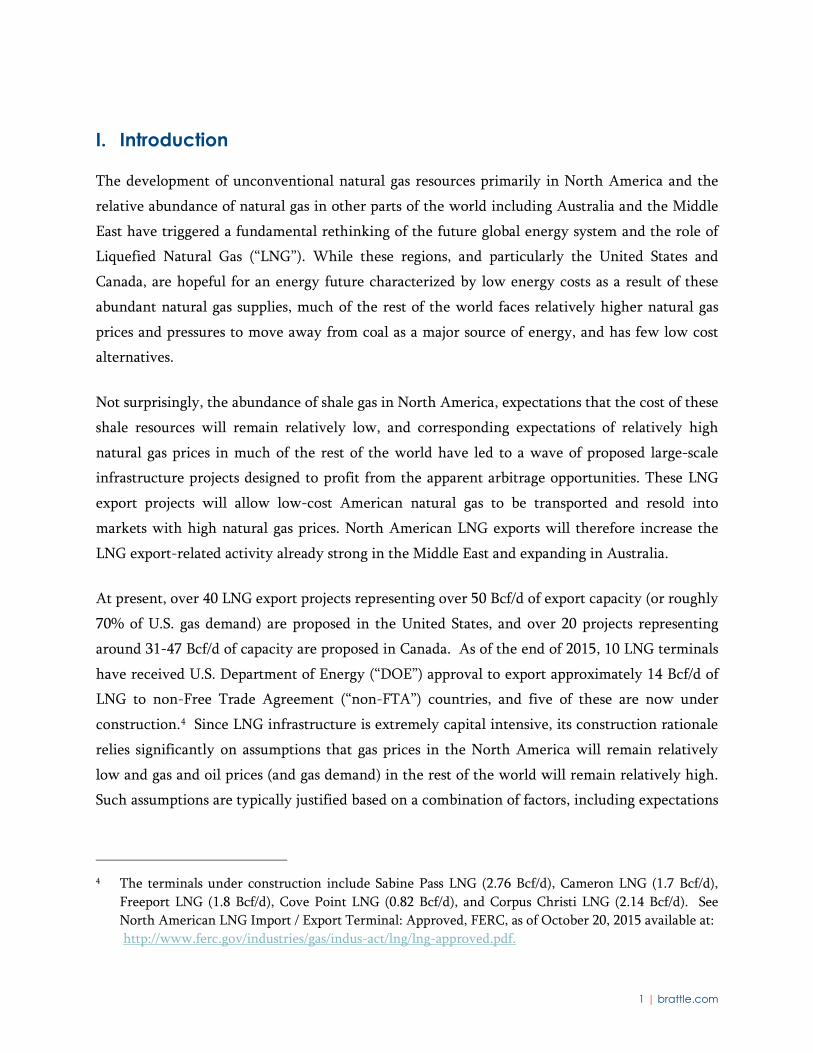
Perhaps the key factor driving these LNG export project proposals was the expectation that the

substantial divergence between North American gas prices and world oil prices that existed until

recently (shown in Figure 1) would persist over the long-term. Since natural gas imports in

many areas (especially in Asian Pacific markets) are priced based on oil market linkages, North

American LNG export developers have been selling LNG export capacity—and hope to sell

additional export capacity—to market participants that could capture this gas-oil spread by

exporting LNG overseas and obtaining an-oil linked price.

Figure 1 NYMEX Prompt Month Prices

Brent Crude Oil vs. Henry Hub Natural Gas January 2000 – November 2015

Sources/Notes: NYMEX data downloaded from EIA and Bloomberg. The natural gas line shows the prompt month Henry Hub prices. The crude oil line shows the prompt month Brent oil prices.

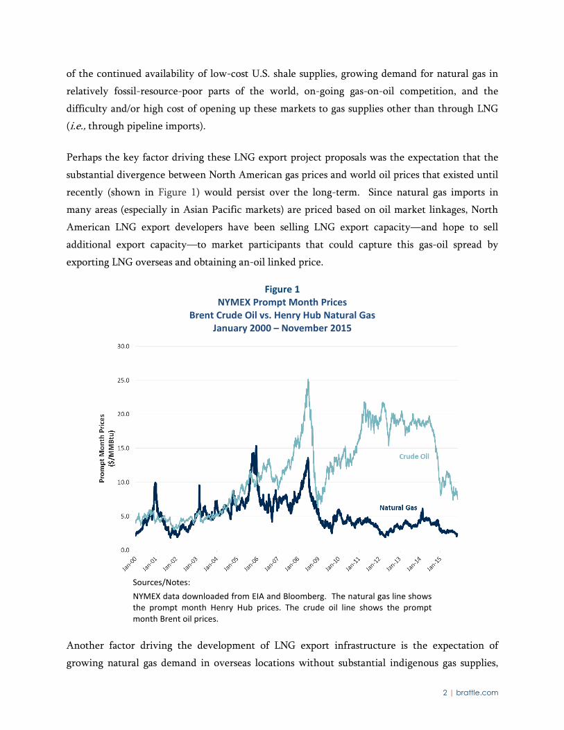
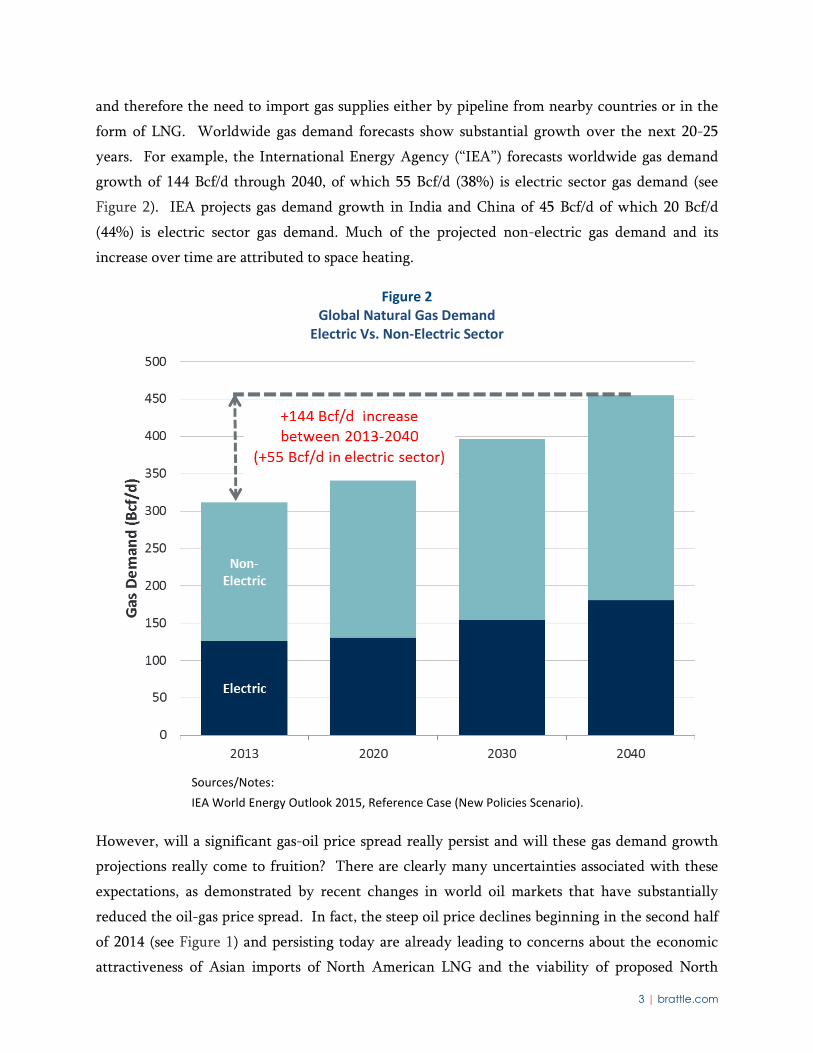
Another factor driving the development of LNG export infrastructure is the expectation of

growing natural gas demand in overseas locations without substantial indigenous gas supplies,

3 | brattle.com

and therefore the need to import gas supplies either by pipeline from nearby countries or in the

form of LNG. Worldwide gas demand forecasts show substantial growth over the next 20-25

years. For example, the International Energy Agency (“IEA”) forecasts worldwide gas demand

growth of 144 Bcf/d through 2040, of which 55 Bcf/d (38%) is electric sector gas demand (see

Figure 2). IEA projects gas demand growth in India and China of 45 Bcf/d of which 20 Bcf/d

(44%) is electric sector gas demand. Much of the projected non-electric gas demand and its

increase over time are attributed to space heating.

Figure 2 Global Natural Gas Demand

Electric Vs. Non-Electric Sector

Sources/Notes: IEA World Energy Outlook 2015, Reference Case (New Policies Scenario).

However, will a significant gas-oil price spread really persist and will these gas demand growth

projections really come to fruition? There are clearly many uncertainties associated with these

expectations, as demonstrated by recent changes in world oil markets that have substantially

reduced the oil-gas price spread. In fact, the steep oil price declines beginning in the second half

of 2014 (see Figure 1) and persisting today are already leading to concerns about the economic

attractiveness of Asian imports of North American LNG and the viability of proposed North

4 | brattle.com

American LNG export projects with Henry-Hub linked pricing.5 Alternatively, shale gas

production in the U.S. could prove to be more costly than now expected, and similarly lead to a

narrowing of this spread. LNG export capability growth could exceed LNG demand (perhaps as

importers lean more heavily on pipeline imports), and such an LNG supply overhang could make

it difficult to achieve oil-linked LNG prices. A worldwide move to more nuclear generation,

technological change (even though appearing relatively unlikely at present), enabling the

development of coal generation with carbon sequestration, a shift from gas to electricity for the

heating sector and, last but not least, more rapid deployment of renewable energy resources,

could limit the need for natural gas.

In this paper, we focus on this last issue, namely on the relative costs of LNG (originating in the

U.S.) and renewables as one important factor impacting future LNG import demand. We explore

the issue by asking a very simple question: How high does the sale price of LNG have to be to

justify investing in LNG infrastructure, and how much competition from renewables might exist

for LNG at that price level? Typically, LNG suppliers think of pricing their product (the LNG

they plan to sell) based on gas-on-oil or gas-on-gas competition. We suggest an alternative view

on the pricing options and constraints for LNG, namely gas-on-renewables competition.

Recognizing that, as illustrated above, a significant portion of the expected growth of natural gas

and hence LNG demand over the coming decades is tied to increasing amounts of electricity

production, we analyze how vulnerable investments in LNG infrastructure or holdings of long-

term LNG export capacity may be to increasing competition from renewable energy sources also

capable of meeting future electricity demand.

For the purposes of this paper, we ignore the possibility of producing incremental electricity

from oil, coal, or nuclear – all real possibilities in various parts of the globe – and focus on

renewable energy sources, which have seen a trend towards declining costs and hence could

increasingly challenge natural-gas fired power generation depending on the costs of gas-fired

generation in the future, of which the LNG price is an important driver.

5 See, for example, “Weak oil threatens US export of LNG, leaving Asian buyers stranded,” Reuters,

October 21, 2014. See also “Moody’s: Liquefied natural gas projects nixed amid lower oil prices,” Moody’s Investors Service, April 7, 2015.

5 | brattle.com

If renewable energy production were to become significantly cheaper than making electricity

from LNG, this would raise some important questions about: a) the risks of buying LNG or LNG

export capacity rights under long-term contracts to meet increasing electricity demand, b) the

risk profile of LNG contracts with various forms of price review and adjustment clauses, and c)

the economic rationale for investments in LNG infrastructure by both equity investors and

lenders.

The remainder of this report explores these questions using a straightforward framework. In the

next section, we briefly summarize our basic assumptions concerning the likely cost of LNG

infrastructure. In Section III we do the same for various types of renewable energy. In Section

IV, we compare the resulting costs of LNG-based and renewable power generation. In Section V,

we discuss the implications of our results. In Section VI, we discuss how electric market

uncertainties and gas market competition are impacting LNG markets, and in Section VII we

draw some conclusions and look forward.

II. The Cost of LNG Infrastructure

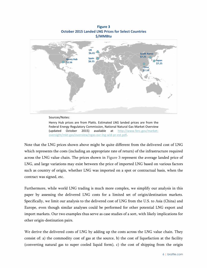
The price paid for LNG by an LNG importer differs by region and source of the LNG imported

(and by contract vintage, as discussed below). Figure 3 below shows the average estimated

landed LNG prices for October 2015 across several countries along with the Henry Hub price in

the U.S. As can be seen, at roughly $7.25/MMBtu6 Asian LNG prices are among the highest in

the world. European prices are slightly lower (around $6.40/MMBtu7), but still significantly

higher than prices in the U.S. The prices shown in Figure 3 are much lower than the prices that

prevailed prior to the recent collapse in oil prices. For example, in November 2013, Asian LNG

prices were around $15-$16/MMBtu, while European prices were $10-$11/MMBtu and U.S.

prices were a little more than $3.00/MMBtu.8

6 Federal Energy Regulatory Commission, National Natural Gas Market Overview (updated October 2015)

available at http://www.ferc.gov/market-oversight/mkt-gas/overview/ngas-ovr-lng-wld-pr-est.pdf. 7 Id. 8 See http://ferc.gov/market-oversight/mkt-gas/overview/2013/10-2013-ngas-ovr-archive.pdf.

6 | brattle.com

Figure 3 October 2015 Landed LNG Prices for Select Countries

$/MMBtu

Sources/Notes: Henry Hub prices are from Platts. Estimated LNG landed prices are from the Federal Energy Regulatory Commission, National Natural Gas Market Overview (updated October 2015) available at http://www.ferc.gov/market-oversight/mkt-gas/overview/ngas-ovr-lng-wld-pr-est.pdf.

Note that the LNG prices shown above might be quite different from the delivered cost of LNG

which represents the costs (including an appropriate rate of return) of the infrastructure required

across the LNG value chain. The prices shown in Figure 3 represent the average landed price of

LNG, and large variations may exist between the price of imported LNG based on various factors

such as country of origin, whether LNG was imported on a spot or contractual basis, when the

contract was signed, etc.

Furthermore, while world LNG trading is much more complex, we simplify our analysis in this

paper by assessing the delivered LNG costs for a limited set of origin/destination markets.

Specifically, we limit our analysis to the delivered cost of LNG from the U.S. to Asia (China) and

Europe, even though similar analyses could be performed for other potential LNG export and

import markets. Our two examples thus serve as case studies of a sort, with likely implications for

other origin-destination pairs.

We derive the delivered costs of LNG by adding up the costs across the LNG value chain. They

consist of: a) the commodity cost of gas at the source, b) the cost of liquefaction at the facility

(converting natural gas to super cooled liquid form), c) the cost of shipping from the origin

7 | brattle.com

country to the destination country, and d) the cost of regasification (converting LNG to natural

gas) and storage at the destination country along with the cost of pipeline transportation from

the regasification facilities to the natural gas consumers (e.g., electric generators). The value

chain is shown in Figure 4.

Figure 4 LNG Value Chain

For our analysis, we use information contained in a NERA Economic Consulting (“NERA”) study

evaluating the economic impacts of U.S. LNG exports9 as the basis for the cost estimates across

each step in the value chain (excluding the commodity cost of gas). This study (referred to as the

“NERA LNG report”) provides forecasts for liquefaction and regasification costs in five year

increments between 2015 and 2035. The NERA LNG report also provides point estimates for

shipping and downstream pipeline costs, which we keep constant in real-value terms during the

forecast period. All of these costs, which are provided in real 2010 dollars ($2010) in the NERA

LNG report, are converted to real 2013 dollars ($2013) using GDP deflator forecasts from EIA’s

Annual Energy Outlook 2015 (“EIA AEO 2015”).10 Together these cost components, including

liquefaction, shipping, re-gasification, and downstream pipeline costs, make up the infrastructure

9 “Macroeconomic Impacts of LNG Exports from the United States,” NERA, December 3, 2012. 10 “Annual Energy Outlook 2015”, EIA, April 14, 2015, available at: http://www.eia.gov/forecasts/aeo/.

8 | brattle.com

costs. The infrastructure cost breakdown for delivered LNG from the U.S. to China/India and

Europe for two representative years, 2015 and 2035, is provided in Figure 5 below.11

Figure 5 Breakdown of Infrastructure Related Delivered LNG Costs from U.S. to Asia and Europe

2015 & 2035 ($2013/MMBtu)

Sources/Notes: “Macroeconomic Impacts of LNG Exports from the United States,” NERA, December 3, 2012. The costs were converted to real 2013 dollars using the GDP deflator forecasts from EIA AEO 2015.

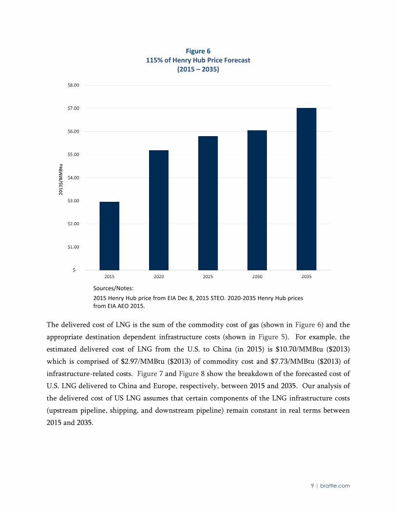
For the cost of feed gas (i.e., the commodity cost of gas) in the U.S., we use the Henry Hub gas

price with a 15% adder.12 The 2015 Henry Hub gas price was obtained from EIA’s December 8,

2015 Short Term Energy Outlook (STEO).13 Henry Hub gas price projections thereafter (2020-

2035) are from EIA AEO 2015. The Henry Hub price forecast (in $2013), inclusive of the 15%

adder, is shown below in Figure 6.

11 Several of the LNG sales contracts for projects in the U.S. Gulf Coast have LNG pricing structures with

a fixed liquefaction fee of around $2.25/MMBtu-$3.50/MMBtu (see, for example, slides 28 and 32 of the Cheniere Energy, Inc. presentation at the December 9, 2015 Capital One Securities Energy Conference). Thus, the forecasted liquefaction costs provided in the NERA LNG report (and reproduced in Figure 5) appear to be towards the lower end of the spectrum.

12 The 15% adder is based on several of the Gulf Coast LNG sales contracts, in which the LNG sales price includes a fixed liquefaction fee plus a variable commodity-based charge of 115% of the Henry Hub natural gas price.

13 The 2015 Henry Hub price reported in the STEO is comprised of historical monthly spot prices between January 2015 and November 2015 and a projected price for December 2015.

China/India Europe China/India Europe

Liquefaction Costs [1] 2.26 2.26 2.47 2.47 Shipping Costs [2] 2.96 1.34 2.96 1.34 Regas and Downstream Pipeline Costs [3] 2.51 1.93 2.52 1.97

Total Infrastructure-Related Costs [4] 7.73 5.53 7.95 5.78

2015 2035

9 | brattle.com

Figure 6 115% of Henry Hub Price Forecast

(2015 – 2035)

Sources/Notes: 2015 Henry Hub price from EIA Dec 8, 2015 STEO. 2020-2035 Henry Hub prices from EIA AEO 2015.

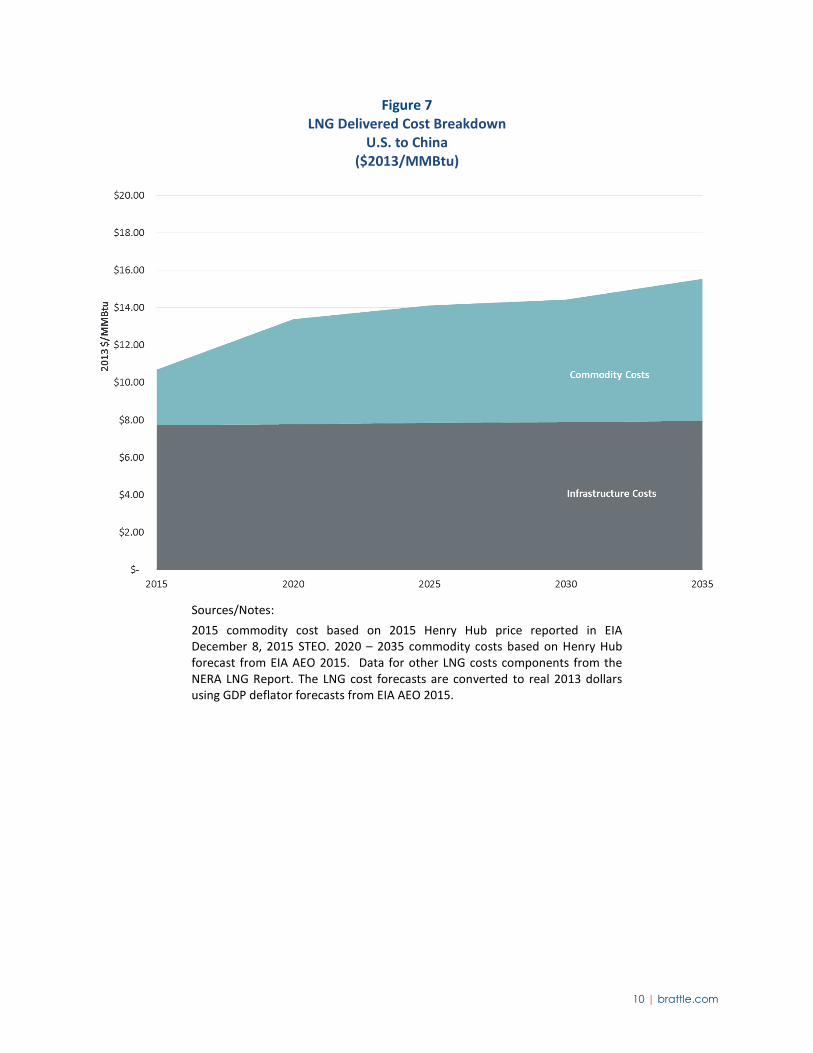
The delivered cost of LNG is the sum of the commodity cost of gas (shown in Figure 6) and the

appropriate destination dependent infrastructure costs (shown in Figure 5). For example, the

estimated delivered cost of LNG from the U.S. to China (in 2015) is $10.70/MMBtu ($2013)

which is comprised of $2.97/MMBtu ($2013) of commodity cost and $7.73/MMBtu ($2013) of

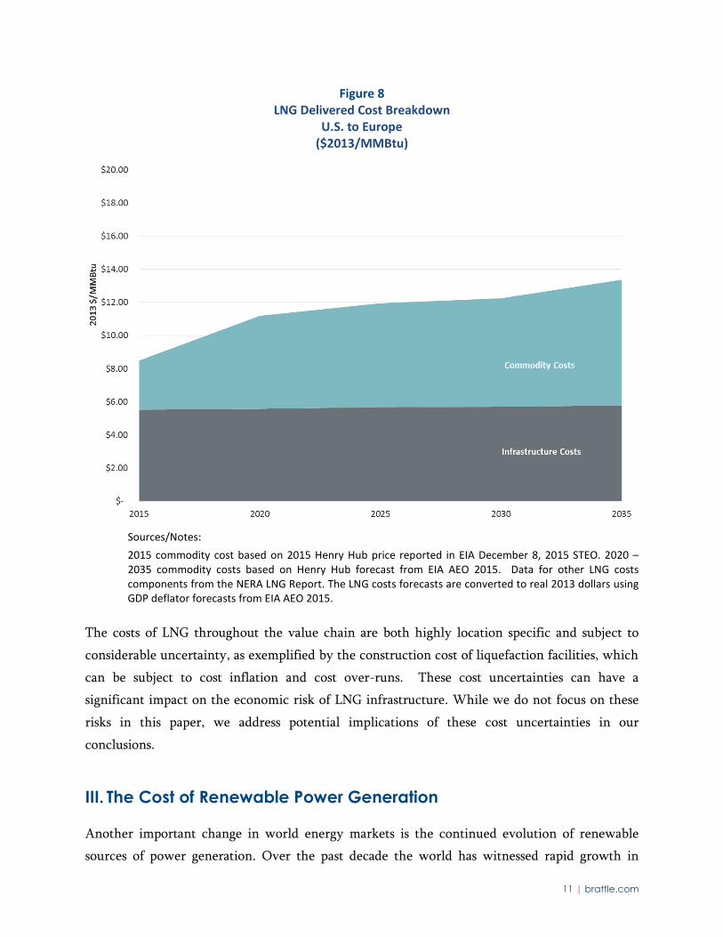
infrastructure-related costs. Figure 7 and Figure 8 show the breakdown of the forecasted cost of

U.S. LNG delivered to China and Europe, respectively, between 2015 and 2035. Our analysis of

the delivered cost of US LNG assumes that certain components of the LNG infrastructure costs

(upstream pipeline, shipping, and downstream pipeline) remain constant in real terms between

2015 and 2035.

10 | brattle.com

Figure 7 LNG Delivered Cost Breakdown

U.S. to China ($2013/MMBtu)

Sources/Notes: 2015 commodity cost based on 2015 Henry Hub price reported in EIA December 8, 2015 STEO. 2020 – 2035 commodity costs based on Henry Hub forecast from EIA AEO 2015. Data for other LNG costs components from the NERA LNG Report. The LNG cost forecasts are converted to real 2013 dollars using GDP deflator forecasts from EIA AEO 2015.

11 | brattle.com

Figure 8 LNG Delivered Cost Breakdown

U.S. to Europe ($2013/MMBtu)

Sources/Notes: 2015 commodity cost based on 2015 Henry Hub price reported in EIA December 8, 2015 STEO. 2020 – 2035 commodity costs based on Henry Hub forecast from EIA AEO 2015. Data for other LNG costs components from the NERA LNG Report. The LNG costs forecasts are converted to real 2013 dollars using GDP deflator forecasts from EIA AEO 2015.

The costs of LNG throughout the value chain are both highly location specific and subject to

considerable uncertainty, as exemplified by the construction cost of liquefaction facilities, which

can be subject to cost inflation and cost over-runs. These cost uncertainties can have a

significant impact on the economic risk of LNG infrastructure. While we do not focus on these

risks in this paper, we address potential implications of these cost uncertainties in our

conclusions.

III. The Cost of Renewable Power Generation

Another important change in world energy markets is the continued evolution of renewable

sources of power generation. Over the past decade the world has witnessed rapid growth in

12 | brattle.com

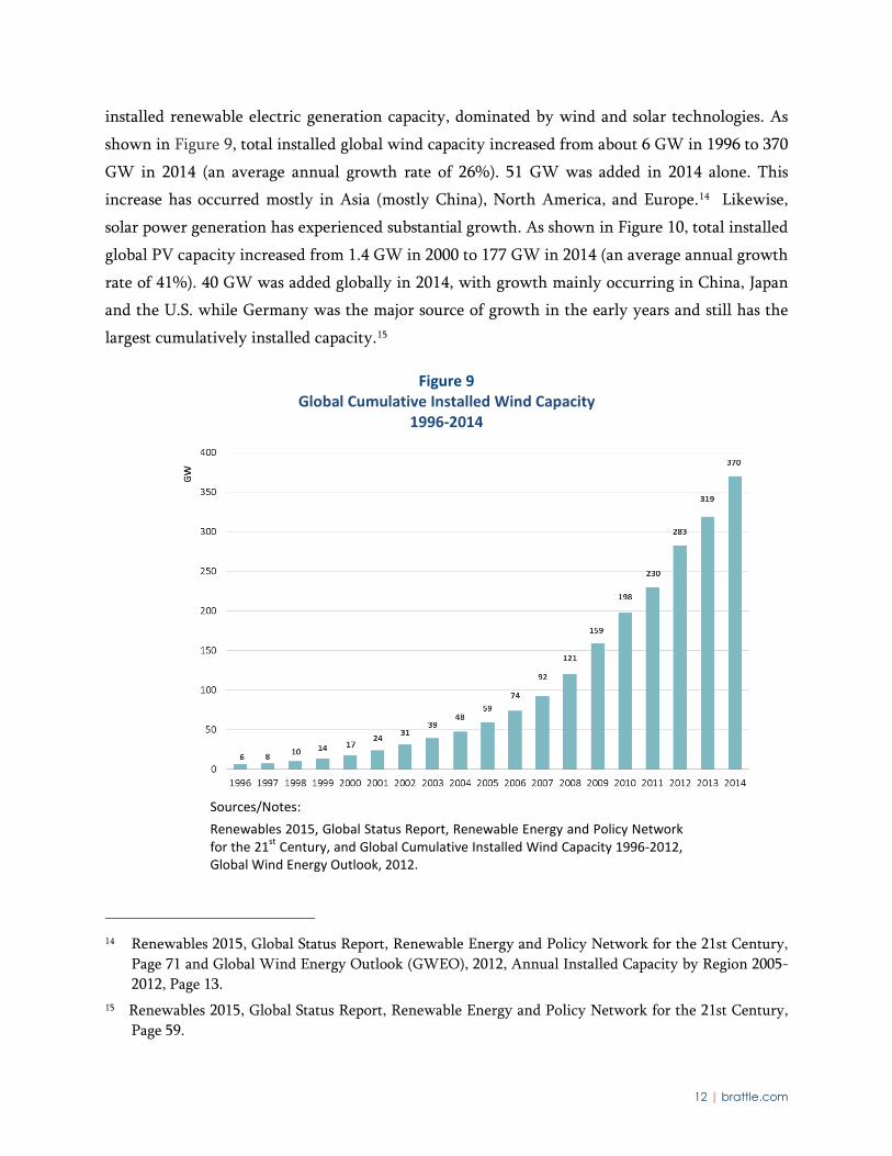
installed renewable electric generation capacity, dominated by wind and solar technologies. As

shown in Figure 9, total installed global wind capacity increased from about 6 GW in 1996 to 370

GW in 2014 (an average annual growth rate of 26%). 51 GW was added in 2014 alone. This

increase has occurred mostly in Asia (mostly China), North America, and Europe.14 Likewise,

solar power generation has experienced substantial growth. As shown in Figure 10, total installed

global PV capacity increased from 1.4 GW in 2000 to 177 GW in 2014 (an average annual growth

rate of 41%). 40 GW was added globally in 2014, with growth mainly occurring in China, Japan

and the U.S. while Germany was the major source of growth in the early years and still has the

largest cumulatively installed capacity.15

Figure 9 Global Cumulative Installed Wind Capacity

1996-2014

Sources/Notes: Renewables 2015, Global Status Report, Renewable Energy and Policy Network for the 21st Century, and Global Cumulative Installed Wind Capacity 1996-2012, Global Wind Energy Outlook, 2012.

14 Renewables 2015, Global Status Report, Renewable Energy and Policy Network for the 21st Century,

Page 71 and Global Wind Energy Outlook (GWEO), 2012, Annual Installed Capacity by Region 2005-2012, Page 13.

15 Renewables 2015, Global Status Report, Renewable Energy and Policy Network for the 21st Century, Page 59.

13 | brattle.com

Figure 10 Global PV Cumulative Installed Capacity

2000 - 2014

Sources/Notes: Renewables 2015, Global Status Report, Renewable Energy and Policy Network for the 21st Century, and Global Market Outlook for Photovoltaic 2013-2017, EPIA.

The cost of generating electricity from these renewables resources has declined significantly over

time, due to technological change and manufacturing advancements, economies of scale, and

performance improvements. For example, since 2009 wind turbine prices have fallen by 20% to

40%. This has contributed significantly to U.S. installed costs falling by $580/kW since 2009 to

$1710/kW in 2014, a reduction 25%.16 Solar PV system costs have fallen by 75% in less than 10

years.17

Despite the small temporary increase in wind generation capital costs between 2005 and 2010

(driven by rising commodity and raw materials prices, increased labor costs, improved

manufacturer profitability, and turbine improvements), the cost of wind generation is expected

to continue to fall (but at a slower pace) given expectations of continued increases in turbine size,

design advancements and possibly lower capital costs. Solar PV costs are expected to continue

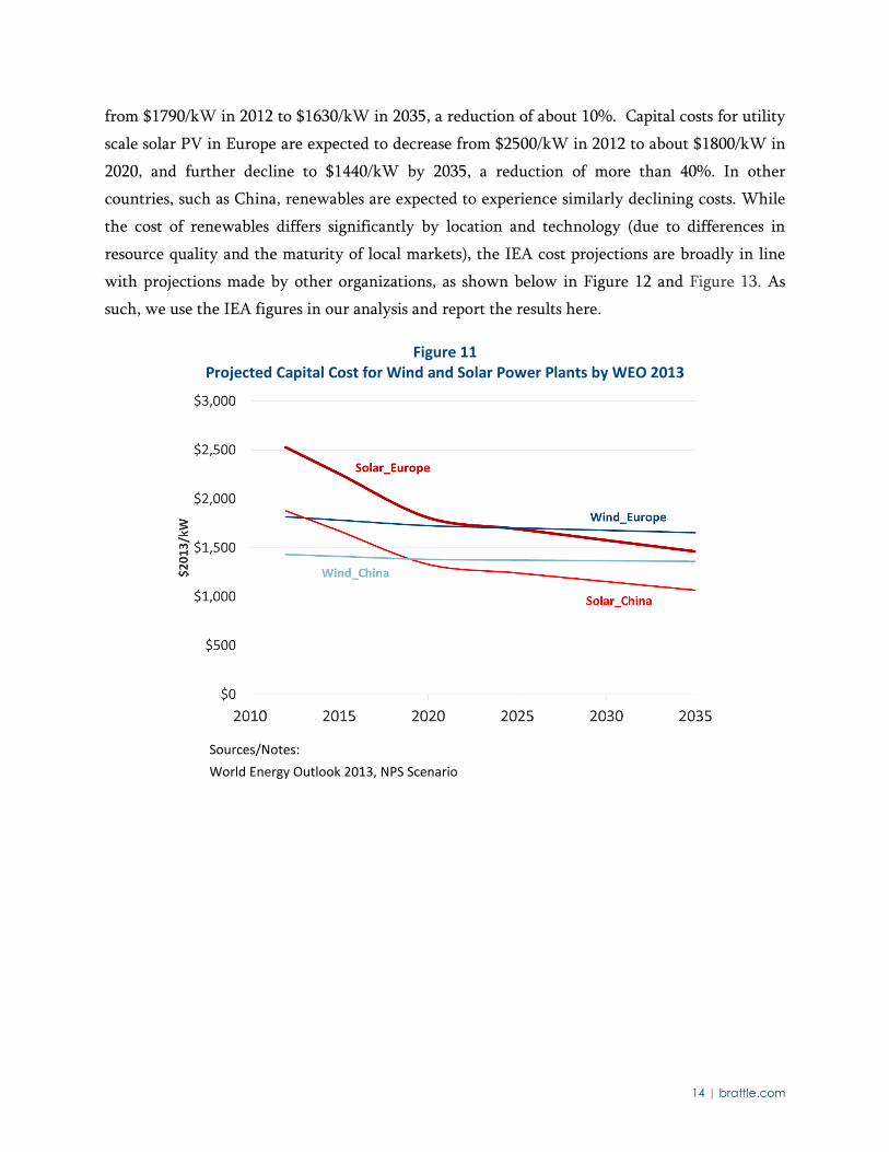
declining more significantly. As shown in Figure 11, according to the World Energy Outlook

2013 published by the IEA, the capital cost of wind projects in Europe is projected to decrease

16 2014 Wind Technologies Market Report, Department of Energy, Aug, 2015. 17 Source: Global Market Outlook For Solar Power / 2015 – 2019, Solar Power Europe, 2014

14 | brattle.com

from $1790/kW in 2012 to $1630/kW in 2035, a reduction of about 10%. Capital costs for utility

scale solar PV in Europe are expected to decrease from $2500/kW in 2012 to about $1800/kW in

2020, and further decline to $1440/kW by 2035, a reduction of more than 40%. In other

countries, such as China, renewables are expected to experience similarly declining costs. While

the cost of renewables differs significantly by location and technology (due to differences in

resource quality and the maturity of local markets), the IEA cost projections are broadly in line

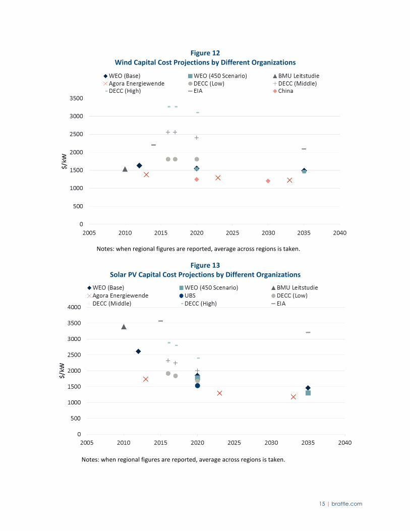
with projections made by other organizations, as shown below in Figure 12 and Figure 13. As

such, we use the IEA figures in our analysis and report the results here.

Figure 11 Projected Capital Cost for Wind and Solar Power Plants by WEO 2013

Sources/Notes: World Energy Outlook 2013, NPS Scenario

15 | brattle.com

Figure 12 Wind Capital Cost Projections by Different Organizations

Notes: when regional figures are reported, average across regions is taken.

Figure 13 Solar PV Capital Cost Projections by Different Organizations

Notes: when regional figures are reported, average across regions is taken.

16 | brattle.com

Although renewables (especially solar) may not have reached grid parity (i.e., a cost that makes

them cost-competitive with incumbent fossil-fuel fired generation) in many markets, and may

not do so for some time, continued technological improvements will likely allow renewables to

increasingly compete with conventional fossil technologies, such as natural gas fired electricity

generation, especially in countries where natural gas prices are high or if natural gas prices

increase over time.

The next section explores the relative economic attractiveness of renewables and natural gas

fired power plants fueled with U.S.-sourced LNG by using China and Germany as examples since

both countries are experiencing rapid development of renewable technologies and have to rely

largely on imported natural gas supplies (including, potentially, imported LNG) for meeting the

fuel requirements of their natural gas fired power plants.

IV. Comparing the Cost of LNG and Renewables

Figure 14, Figure 15, and Figure 16 combine the insights from the above two sections by

comparing the forecast delivered cost of U.S.-sourced LNG (shaded regions) expressed in

$/MMBtu with the equivalent cost of wind, solar and a combination of wind and solar, also

expressed in $/MMBtu, (i.e., as the price of natural gas at which the respective technologies

break even).18 As described above, actual landed prices may be quite different from the delivered

cost of LNG. In the analysis below, we use the forecasted delivered cost of LNG (including all

infrastructure costs) as a proxy for the price of LNG. As long as the delivered cost of LNG is

below the break-even prices for renewables (expressed in $/MMBtu), generating electricity using

LNG would be less expensive than generating power from renewable sources. Conversely, if the

delivered cost of LNG is above the break-even prices for renewables, then generating electricity

using renewables would be less expensive than generating power from LNG.

18 First, we calculate the levelized cost of electricity (LCOE) for renewables in $/MWh using assumed

capital costs, fixed operations and maintenance (FOM) costs and renewable capacity factors. We then transform this LCOE in $/MWh into an equivalent gas price in $/MMBtu by calculating the natural gas price that makes the LCOE (in $/MWh) of a new combined cycle gas plant equal to the calculated LCOE for renewables in $/MWh (using assumed capital costs, FOM, VOM, and heat rate of a new gas-fired combined cycle power plant).

17 | brattle.com

Figure 14 Breakeven Analysis for Wind Renewables and New Gas-Fired Combined Cycle in China Based on

Forecast Delivered Cost of LNG from U.S. to China

Sources/Notes: World Energy Outlook 2013 for renewables cost assumptions (NPS Scenario). Delivered LNG cost breakdown from Figure 7.

As can be seen from Figure 14, it appears that generating power in China using wind with a

capacity factor of 25% or greater would already be competitive with generating power with new

combined cycle gas turbines using LNG. Such wind capacity factors are not unrealistic for some

locations in China.19 By 2020 or 2025, about the time when many of LNG projects now under

consideration (but that have not yet advanced to construction) might be able to deliver LNG,

wind with a capacity factor of 20% becomes competitive with generation using LNG. Based on

this simplified analysis, capacity factors of between 20% and 25% would suffice for wind to be

cheaper than LNG over the typical LNG contract length of 20 years.

19 McElroy, Michael B., Xi Lu, Chris P. Nielsen, and Yuxuan, Wang. 2009. Potential for wind-generated

electricity in China, Science 325(5946): 1378-1380, Figure 1.

18 | brattle.com

Figure 15 Breakeven Analysis for Solar PV and New Gas-Fired Combined Cycle in China

Based on Forecast Delivered Cost of LNG from U.S. to China

Sources/Notes: World Energy Outlook 2013 for renewables cost assumptions (NPS Scenario). Delivered LNG cost breakdown from Figure 7.

Figure 15 shows that electricity generation from solar PV is more expensive than generation

from new gas-fired plants using LNG through approximately 2020 unless the solar capacity factor

is 20% or higher. But if technology development reduces the cost for solar and gas prices increase

over time, solar with a capacity factor of 15% could become competitive with gas before 2035.

However, this does not mean that solar with a capacity factor of 15% should not be considered

competitive relative to a gas-fired plant before 2035. The reason is that solar can complement

wind in that wind speeds tend to be lower in the summer (in the northern hemisphere) when

the sun shines brightest and longest, and wind tends to be strong in the winter when less

sunlight is available. Consequently, since the peak operating times for wind and solar systems

occur at different times of the day and year, a hybrid system might better match with demand

than wind or solar PV facilities by themselves. To illustrate how this could affect the

competitiveness of wind and solar as compared to a natural gas power plant, we constructed a

19 | brattle.com

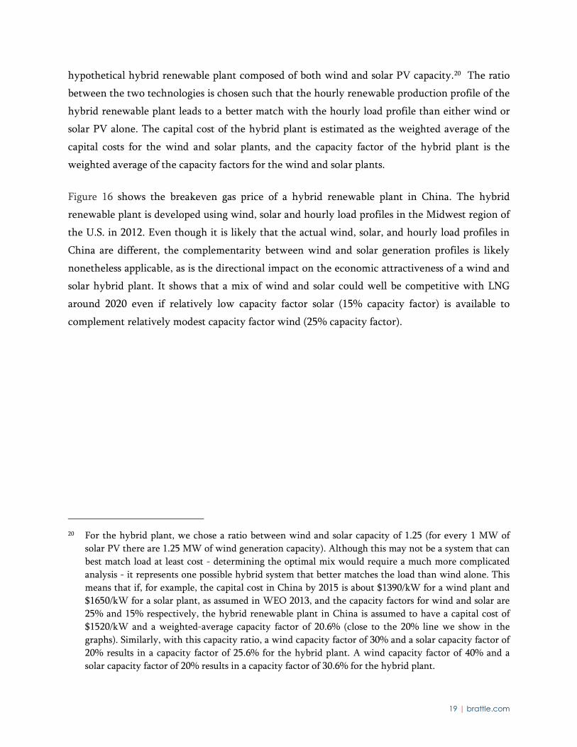
hypothetical hybrid renewable plant composed of both wind and solar PV capacity.20 The ratio

between the two technologies is chosen such that the hourly renewable production profile of the

hybrid renewable plant leads to a better match with the hourly load profile than either wind or

solar PV alone. The capital cost of the hybrid plant is estimated as the weighted average of the

capital costs for the wind and solar plants, and the capacity factor of the hybrid plant is the

weighted average of the capacity factors for the wind and solar plants.

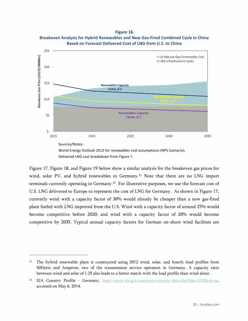
Figure 16 shows the breakeven gas price of a hybrid renewable plant in China. The hybrid

renewable plant is developed using wind, solar and hourly load profiles in the Midwest region of

the U.S. in 2012. Even though it is likely that the actual wind, solar, and hourly load profiles in

China are different, the complementarity between wind and solar generation profiles is likely

nonetheless applicable, as is the directional impact on the economic attractiveness of a wind and

solar hybrid plant. It shows that a mix of wind and solar could well be competitive with LNG

around 2020 even if relatively low capacity factor solar (15% capacity factor) is available to

complement relatively modest capacity factor wind (25% capacity factor).

20 For the hybrid plant, we chose a ratio between wind and solar capacity of 1.25 (for every 1 MW of

solar PV there are 1.25 MW of wind generation capacity). Although this may not be a system that can best match load at least cost - determining the optimal mix would require a much more complicated analysis - it represents one possible hybrid system that better matches the load than wind alone. This means that if, for example, the capital cost in China by 2015 is about $1390/kW for a wind plant and $1650/kW for a solar plant, as assumed in WEO 2013, and the capacity factors for wind and solar are 25% and 15% respectively, the hybrid renewable plant in China is assumed to have a capital cost of $1520/kW and a weighted-average capacity factor of 20.6% (close to the 20% line we show in the graphs). Similarly, with this capacity ratio, a wind capacity factor of 30% and a solar capacity factor of 20% results in a capacity factor of 25.6% for the hybrid plant. A wind capacity factor of 40% and a solar capacity factor of 20% results in a capacity factor of 30.6% for the hybrid plant.

20 | brattle.com

Figure 16 Breakeven Analysis for Hybrid Renewables and New Gas-Fired Combined Cycle in China

Based on Forecast Delivered Cost of LNG from U.S. to China

Sources/Notes: World Energy Outlook 2013 for renewables cost assumptions (NPS Scenario), Delivered LNG cost breakdown from Figure 7.

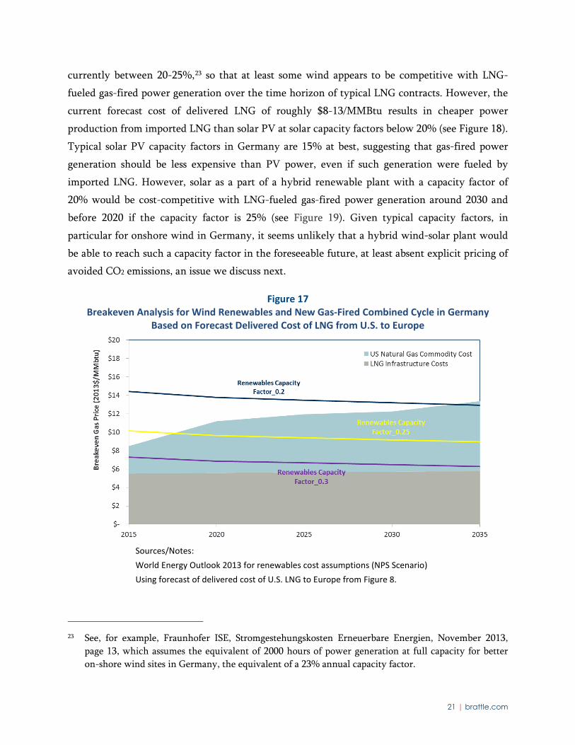
Figure 17, Figure 18, and Figure 19 below show a similar analysis for the breakeven gas prices for

wind, solar PV, and hybrid renewables in Germany.21 Note that there are no LNG import

terminals currently operating in Germany.22 For illustrative purposes, we use the forecast cost of

U.S. LNG delivered to Europe to represent the cost of LNG for Germany. As shown in Figure 17,

currently wind with a capacity factor of 30% would already be cheaper than a new gas-fired

plant fueled with LNG imported from the U.S. Wind with a capacity factor of around 25% would

become competitive before 2020; and wind with a capacity factor of 20% would become

competitive by 2035. Typical annual capacity factors for German on-shore wind facilities are

21 The hybrid renewable plant is constructed using 2012 wind, solar, and hourly load profiles from

50Hertz and Amprion, two of the transmission service operators in Germany, A capacity ratio between wind and solar of 1.25 also leads to a better match with the load profile than wind alone.

22 EIA Country Profile - Germany, http://www.eia.gov/countries/country-data.cfm?fips=GM&trk=m, accessed on May 6, 2014.

21 | brattle.com

currently between 20-25%,23 so that at least some wind appears to be competitive with LNG-

fueled gas-fired power generation over the time horizon of typical LNG contracts. However, the

current forecast cost of delivered LNG of roughly $8-13/MMBtu results in cheaper power

production from imported LNG than solar PV at solar capacity factors below 20% (see Figure 18).

Typical solar PV capacity factors in Germany are 15% at best, suggesting that gas-fired power

generation should be less expensive than PV power, even if such generation were fueled by

imported LNG. However, solar as a part of a hybrid renewable plant with a capacity factor of

20% would be cost-competitive with LNG-fueled gas-fired power generation around 2030 and

before 2020 if the capacity factor is 25% (see Figure 19). Given typical capacity factors, in

particular for onshore wind in Germany, it seems unlikely that a hybrid wind-solar plant would

be able to reach such a capacity factor in the foreseeable future, at least absent explicit pricing of

avoided CO2 emissions, an issue we discuss next.

Figure 17 Breakeven Analysis for Wind Renewables and New Gas-Fired Combined Cycle in Germany

Based on Forecast Delivered Cost of LNG from U.S. to Europe

Sources/Notes: World Energy Outlook 2013 for renewables cost assumptions (NPS Scenario) Using forecast of delivered cost of U.S. LNG to Europe from Figure 8.

23 See, for example, Fraunhofer ISE, Stromgestehungskosten Erneuerbare Energien, November 2013,

page 13, which assumes the equivalent of 2000 hours of power generation at full capacity for better on-shore wind sites in Germany, the equivalent of a 23% annual capacity factor.

22 | brattle.com

Figure 18 Breakeven Analysis for Solar Renewables and New Gas-Fired Combined Cycle in Germany

Based on Forecast Delivered Cost of LNG from U.S. to Europe

Sources/Notes: World Energy Outlook 2013 for renewables cost assumptions (NPS Scenario) Using forecast of delivered cost of U.S. LNG to Europe from Figure 8.

Figure 19 Breakeven Analysis for Hybrid Renewables and New Gas-Fired Combined Cycle in Germany

LNG Delivered Cost Breakdown from U.S. to Germany

Sources/Notes: World Energy Outlook 2013 for renewables cost assumptions (NPS Scenario) Using forecast of delivered cost of U.S. LNG to Europe from Figure 8.

23 | brattle.com

Including the cost of carbon emissions associated with gas-fired power generation would make

gas-fired power generation more expensive relative to renewables. While there is a lot of

uncertainty about the price of carbon in Europe going forward, the European Union’s (EU)

ambitious long-term GHG reduction goals and past EU Emission Trading Scheme (ETS) prices

suggest that a price of $30/ton of CO2 to illustrate the impacts of carbon prices on the

competitiveness between renewables and LNG in Germany is reasonable.24 An allowance price of

$30/ton of CO2 would add about $1.60/MMBtu to the cost of LNG, or about $10/MWh for the

electricity generated from a new gas-fired combined cycle plant with a heat rate of about 6,200

Btu/kWh (as assumed by WEO 2013). This results in the breakeven prices shown in Figure 20.

As shown, at a $30/ton carbon price, a hybrid renewable plant with a capacity factor of 20%

(achievable for example with a combination of wind at a capacity factor of 25% and solar at a

capacity factor of 15%) would be competitive with an LNG-fueled gas-fired plant before 2025,

about 5 years earlier than without the inclusion of the value of avoided greenhouse gas

emissions.

24 Allowance prices under the European Union Emissions Trading Scheme (“EU ETS”) ranged between

€20 and €30/ton of CO2 prior to the financial crisis of 2008. $30/ton corresponds to approximately €22/ton at current exchange rates. While current prices under the EU ETS are far below this historic level, there is widespread agreement that low current allowance prices are not reflective of the levels needed to achieve the EU’s longer term carbon reduction goals.

24 | brattle.com

Figure 20 Breakeven Analysis for Hybrid and New Gas-Fired Combined Cycle in Germany with Carbon

Emissions’ Cost of $30/ton Based on Forecast Delivered Cost of LNG from U.S. to Europe

Sources/Notes: World Energy Outlook 2013 for renewables cost assumptions (NPS Scenario) Using forecast of delivered cost of U.S. LNG to Europe from Figure 8.

Figure 20 shows that pricing GHG emissions could further tip the scale in favor of renewable

energy sources even in places such as Germany, where neither wind nor solar PV resource

quality is very high.25 When and how highly GHG emissions will be valued (either explicitly

through the creation of carbon markets or carbon taxes or indirectly through policy making that

impacts of the choice of generation mix) therefore has a significant impact on how quickly

renewable energy sources might gain a cost advantage over LNG-based power generation. Very

recent developments in China26 leading up to the Conference of Parties (COP) in Paris in

December 2015 suggest that pricing GHG emissions may happen sooner rather than later.

25 Recent U.S. onshore wind projects in the Midwest are achieving capacity factors in excess of 50%.

Solar PV plants in the Southwestern United States can achieve capacity factors between 20% and 25%. Some of the difference is due to different resource quality (more wind, more sun), but some is also a reflection of ongoing technological advances, which will likely lead to increased capacity factors of new wind and solar PV resources in Germany as well.

26 China to Announce Cap-and-Trade Program to Limit Emissions,

Continued on next page

25 | brattle.com

V. Discussion

The above analysis shows that renewable energy may be able to compete with imported LNG

under a number of conditions in the near future and most likely during the lifetime of the long-

term LNG contracts supporting new LNG export infrastructure (i.e., contracts that have already

been negotiated for new export terminals now under construction as well as contracts being

pursued by export terminals currently in the development phase). Advances in renewable

energy technology and related cost improvements, which are further helped by an increasingly

mature supply chain, economies of scale and increased competition, could result in renewables

putting competitive pressure on LNG as a source of fuel in the electric generation sector in many

target markets for North American LNG. Such competitive pressure could lead to lower demand

for LNG relative to current forecasts, and lower prices for LNG in world markets, all else equal.

In areas with good conditions for renewable energy production (high average wind speeds and/or

high solar irradiation) renewable energy is already beginning to compete with fossil generation,

even at relatively low natural gas prices and generally with low or no price on carbon. Evidence

of this competition can be seen in some of the recently signed long-term renewable contracts in

the United States – where gas prices are amongst the lowest in the world – at prices that are

deemed to be lower than those from competing fossil fuels, and in particular gas-fired generation

projects. For example, in 2014 the national average levelized price of wind PPAs that were signed

fell to around $23.5/KWh in the U.S.27 PPAs for solar PV projects have also decreased

significantly, with some evidence that in good locations long-term contracts can be obtained at

prices below $40/MWh.28 Even if existing subsidies for renewable energy sources are netted out

of these prices,29 renewable energy sources in these examples would in the worst case not be

Continued from previous page

http://www.nytimes.com/2015/09/25/world/asia/xi-jinping-china-president-obama-summit.html?_r=0.

27 See, for example, U.S. Department of Energy, 2014 Wind Technologies Market Report, August 2015, page 56.

28 http://www.utilitydive.com/news/nv-energy-buys-utility-scale-solar-at-record-low-price-under-4-centskwh/401989/, accessed on October 7, 2015.

29 Solar PV projects benefit from an investment tax credit covering 30% of the investment costs. Until year-end 2013, wind projects benefitted from a production tax credit of 23 cents/kWh, and all renewable projects benefit from accelerated depreciation allowances.

26 | brattle.com

significantly more expensive than power from new gas-fired generation, and in many cases

cheaper. In this sense, the recent experience in the United States is an illustration of the

declining break-even cost of renewable alternatives to natural gas fired power generation.

These trends in the costs of renewables suggest some risks associated with the use of LNG for gas-

fired power generation in overseas markets, and for purchasers of LNG under long-term

contracts who may be counting on strong world LNG demand for power generation based on the

presumption that power generation using LNG will be cheaper than non-gas generation

alternatives such as renewables. We discuss these risks and uncertainties in the next section.

It is, however, important to recognize that our analysis is deliberately simple and thus omits

factors that would likely move the relative cost of imported LNG versus renewables one way or

the other. Several factors would have the tendency to improve the value of imported LNG when

compared to renewables relative to our simple analysis above.

First and foremost, the results presented above illustrate that the ability of renewable energy to

outcompete imported LNG depends critically on the quality of the available renewable resource.

In many cases, the ideal locations for renewable energy sources will not be close to load centers,

so that potentially significant additional costs will be incurred to bring such resources to market,

even if sufficient locations with good resource quality are available. As a case in point, bringing

large amounts of high-quality wind power in China to market will likely require very significant

investments in additional transmission infrastructure, as the best wind resources are located in

the very Western and Northern parts of China, whereas the demand centers are located in the

East and South. Corresponding incremental infrastructure costs are likely less important for LNG

imports, since large demand centers are often located near the coast and hence LNG

infrastructure can be located in relative proximity. Gas-fired power generation can also be

located near the coast and the resulting electric transmission to bring power from such plants to

load centers will often be less expensive than building transmission infrastructure from Western

China to the coast. Hence, if the costs of connecting high quality renewables to demand centers

are high, the actual cost of renewables will likely be higher than our estimates.

A second often discussed issue relates to the intermittency of renewable generation and the

“integration” costs required to manage the disconnect between renewable generation and

demand in contrast with gas-fired generation, which can serve demand reliably and be

controlled to reflect fluctuating demand. The level of renewable integration costs depends on

the mix of renewable resources used, the amount of renewable energy generation and the shape

27 | brattle.com

of the demand. Also, market structures and the available technology to integrate renewables

matter. For example, advances in battery technology and associated costs may well lead to lower

integration costs in the future. A number of studies have attempted to estimate integration costs

as a function of the various factors cited above. In general, cost estimates have shown a range of

approximately $2-5 per MWh of renewable generation.30 This translates to a range of $0.3-

0.8/MMBtu, which suggests that, at least at moderate penetration levels, including renewable

integration costs would likely not fundamentally alter the results of our analysis. At high levels

of renewable generation, integration costs could become much more significant, and

consequently the economics of renewables relative to LNG could deteriorate significantly absent

cost reductions for enabling technology corresponding to cost reductions for renewable energy

itself.31

Third, while our comparison of LNG and renewables accounted for expected declines in the cost

of renewables, it did not assume reductions in the cost of gas-fired generation or LNG supply

chain costs. For example, some project developers in Australia are now considering floating

liquefaction projects as a potentially less expensive alternative to onshore LNG projects (with

potential savings on the order of 20-30%).32 Such savings in the cost of LNG export projects or in

other parts of the LNG supply chain could improve the economics of LNG relative to renewables.

Fourth, the cost of feed gas for LNG (i.e., the commodity cost of gas) is itself uncertain and will

depend upon various factors including the potential for additional technological improvements

in the production of natural gas. The uncertainty in the commodity cost of gas directly affects the

relative attractiveness of renewables and LNG. If, for example, the commodity cost of gas in the

U.S. is lower than the projections we have assumed (resulting in a lower delivered cost of LNG),

LNG can become more competitive with renewables in LNG destination markets such as China.

30 See, for example, Michael Milligan, Wind Integration Cost and Ancillary Service Impacts,

presentation, August 10, 2006, which cites many previous studies. Since then, many additional studies have been conducted. One main conclusion is that renewable integration costs increase potentially sharply above some minimum threshold of overall renewable energy penetration.

31 It should however be noted that as the deployment of variable renewable generation has increased, so has the ability to integrate these resources through a mix of operational changes, market rule changes, and technology. As a consequence, the penetration threshold of renewable resources that would result in significantly higher integration costs will likely continue to increase.

32 See “High-Cost Australia May Miss $180 bln LNG Expansion Wave,” Reuters, April 11, 2014.

28 | brattle.com

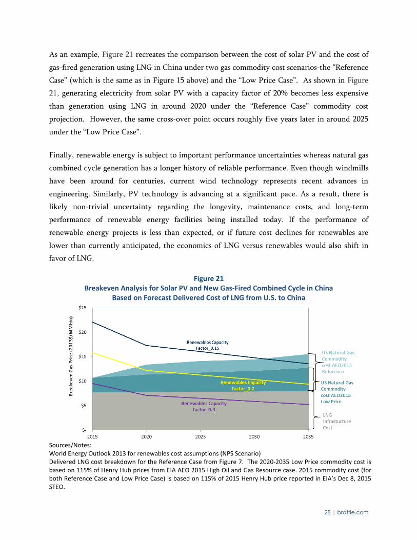
As an example, Figure 21 recreates the comparison between the cost of solar PV and the cost of

gas-fired generation using LNG in China under two gas commodity cost scenarios-the “Reference

Case” (which is the same as in Figure 15 above) and the “Low Price Case”. As shown in Figure

21, generating electricity from solar PV with a capacity factor of 20% becomes less expensive

than generation using LNG in around 2020 under the “Reference Case” commodity cost

projection. However, the same cross-over point occurs roughly five years later in around 2025

under the “Low Price Case”.

Finally, renewable energy is subject to important performance uncertainties whereas natural gas

combined cycle generation has a longer history of reliable performance. Even though windmills

have been around for centuries, current wind technology represents recent advances in

engineering. Similarly, PV technology is advancing at a significant pace. As a result, there is

likely non-trivial uncertainty regarding the longevity, maintenance costs, and long-term

performance of renewable energy facilities being installed today. If the performance of

renewable energy projects is less than expected, or if future cost declines for renewables are

lower than currently anticipated, the economics of LNG versus renewables would also shift in

favor of LNG.

Figure 21 Breakeven Analysis for Solar PV and New Gas-Fired Combined Cycle in China

Based on Forecast Delivered Cost of LNG from U.S. to China

Sources/Notes: World Energy Outlook 2013 for renewables cost assumptions (NPS Scenario) Delivered LNG cost breakdown for the Reference Case from Figure 7. The 2020-2035 Low Price commodity cost is based on 115% of Henry Hub prices from EIA AEO 2015 High Oil and Gas Resource case. 2015 commodity cost (for both Reference Case and Low Price Case) is based on 115% of 2015 Henry Hub price reported in EIA’s Dec 8, 2015 STEO.

29 | brattle.com

However, there are also factors that could shift the balance further in favor of renewables. First,

unlike renewable energy sources, which can be scaled from just a few kW for single rooftop solar

PV systems or a few MWs for small wind projects to 100s of MWs for large wind or solar farms,

traditional onshore LNG infrastructure projects represent huge one-time commitments of capital

and result in hyper-complex building projects such as those in Australia, where the most

expensive projects have capital costs ranging from $30-$60 billion. There is significant evidence

that with large single infrastructure projects the risks of cost-overruns and completion delays are

substantial. In fact, several of the Australian LNG projects have experienced significant cost-

overruns. Both cost-overruns and construction delays can have substantial, negative effects on

the economics of such projects, although some contracting practices (such as cost-sharing

provisions) can help mitigate these impacts. These types of cost-overrun risks are not accounted

for in our analysis.

Second, as discussed above, the environmental advantages of renewables and the potential

inclusion of carbon costs in the future would further improve the economics of renewables

relative to LNG, as shown in our analysis of Germany. However, it is important to mention that

climate change considerations work against imported LNG if imported LNG is assumed to

displace renewable energy production. If, on the other hand, LNG imports were to displace new

or existing coal-fired generation, LNG imports could provide a significant and positive

contribution towards reducing greenhouse gas emissions. Of course for LNG to displace coal but

not renewable energy (even in cases where our charts show renewable energy may be cheaper)

would require that LNG would be cheaper than coal, but that somehow even cheaper renewable

energy does not displace coal. While this would seem unlikely in theory, it may well be the case

in practice, due to any number of factors, many of which are likely very location/country and

context specific, such as the fact that the time required to get new transmission infrastructure for

renewable energy planned, approved, financed and built may be significantly longer than the

time required to build new coal-fired generation or the fear that renewable energy may not be

“reliable” enough to displace traditional fossil power generation sources.

To summarize, while the relatively simple analysis presented in this paper leaves out important

factors affecting the relative attractiveness of LNG-fueled and renewable power generation, it

does not appear that the omission of these factors clearly bias our results one way or another.

30 | brattle.com

VI. Electric Market Uncertainties and Gas Market Competition: Implications for LNG Markets

The electric power sector is a critical sector impacting worldwide natural gas and LNG markets.

Uncertainty regarding the future mix of electric generation capacity creates uncertainty in

demand for natural gas and LNG. Thus, developments in the electric sector have important

ramifications for natural gas markets. The competition between gas-fired generation capacity

and other types of power plants (renewables as discussed in this paper, but also potentially

nuclear) creates risks for participants in natural gas and LNG markets.

Forecasts of LNG demand (as distinct from natural gas demand) made prior to the recent oil price

collapse projected LNG demand growth from current levels of about 32 Bcf/d to levels of 65-85

Bcf/d by 2030 (i.e., growth of 33 to 53 Bcf/d).33 More recent forecasts of LNG trade (following

the collapse in oil prices) have varied widely. For example, BP’s Energy Outlook 2035 (released

in February 2015) projected LNG demand to grow from 32 Bcf/d to roughly 70 Bcf/d by 2030 and

to approximately 80 Bcf/d in 2035.34 IEA’s World Energy Outlook 2015 (released in November

2015) projects significantly lower growth in LNG trade, to approximately 40 Bcf/d by 2025 and to

roughly 50 Bcf/d by 2040 (i.e., growth on the order of roughly 18 Bcf/d between now and

2040).35 The uncertainty in LNG demand, as shown by this range of forecasts, is substantial.

Reduced gas demand in the power sector, as a consequence of the factors described in this paper

(which could also include more nuclear generation in addition to a shift towards more

renewables, as a result of cost and/or climate change issues), could have a significant impact on

overall LNG demand and thus the need for LNG liquefaction terminals. For example, a 6 Bcf/d

reduction in LNG demand would be the equivalent of three to six fewer LNG liquefaction

terminals (assuming an average LNG terminal size of 1.0-2.0 Bcf/d).

In general, the uncertainties in the electric power sector, especially in Asian markets, combined

with other uncertainties are creating significant risks in global LNG markets. In the near-term,

global LNG markets can be characterized as a buyer’s market due to the oversupply conditions

33 See, for example, “US Manufacturing and LNG Exports, Economic Contributions to the US Economy

and Impacts on US Natural Gas Prices,” Charles River Associates, February 25, 2013, page 31. 34 See BP Energy Outlook 2035, slide 56. 35 IEA World Energy Outlook 2015, Reference Case (New Policies Scenario), page 220.

31 | brattle.com

that have developed recently. Spot LNG prices in the aftermath of the oil price collapse have

converged globally to the $7/MMBtu range. Gas demand growth has slowed in key Asian and

European markets for a variety of reasons, including mild winters, the availability of cheap coal,

the development of renewable resources, and slower economic growth. In addition, new LNG

supplies have started to come online, such as the Queensland Curtis Island LNG project in

eastern Australia. These conditions may persist or worsen over the next several years as a

substantial amount of additional new LNG liquefaction capacity is set to enter service both in

Australia (8 Bcf/d of new liquefaction capacity) and the U.S. (9 Bcf/d) between 2015 and 2020. A

restart of some of Japan’s nuclear fleet may also result in lower LNG demand for power

generation by Japan, further contributing to the oversupply situation in the next few years.

Thus, the questions facing global LNG markets today are how quickly the new LNG supplies

coming on line over the next few years will be absorbed, and at what point in the future there

might be a rebound in global LNG prices such that new LNG export terminals (beyond the

terminals now under construction) are needed. Many market observers believe the answers to

these questions will hinge on how gas demand growth (including electric sector demand)

develops in Pacific Asian markets, especially markets in China and India. In addition to the

dynamic of renewables versus gas competition discussed in detail in this paper, other important

factors include overall economic growth in these markets and competition to serve growing gas

demand in Asian markets from pipeline imports and indigenous supply sources. A recent

example of this competition can be seen in China’s decision in May 2014 to enter into a long-

term contract for pipeline gas from Russia. The deal is reported to be a 30-year contract under

which Russia will supply China with approximately 3.7 Bcf/d of natural gas (roughly the size of

1-2 LNG export terminals), at a price in the range of $9-$11/MMBtu.36 A second (non-binding)

deal between China and Russia was signed in November 2014, also reported to be a 30-year

contract under which Russia will supply China with an additional 2.9 Bcf/d of natural gas.37

China is also understood to have substantial indigenous shale gas resources, but is only in the

early stages of developing those resources.

36 “Sino-Russian Gas and Oil Cooperation: Entering into a New Era of Strategic Partnership?” Oxford

Energy Institute, April 2015, pp. 7-8. 37 Id., pp. 8-10.

32 | brattle.com

From the North American perspective, the current market conditions and future uncertainties

create various risks. The five LNG liquefaction terminals now under construction in the US have

largely shielded themselves from these risks by signing long-term offtake contracts with LNG

buyers. The US LNG offtake agreements are typically structured such that the purchaser agrees

to take LNG at the tailgate of an LNG export plant, at a price linked to Henry Hub (usually

multiplied by a scalar, e.g. 115% of Henry Hub), plus a fixed infrastructure charge to cover

liquefaction in the range of $3/MMBtu. Thus, the energy companies signing contracts for U.S.-

based LNG are assuming the risk that Henry Hub prices may become uneconomic in world

markets, in which case they can forgo exporting LNG from the US, but still have to pay the

infrastructure charge to the LNG developers (which must be paid even if the buyer does not take

LNG from the facility). Thus, it is the LNG buyers in these long-term agreements that are

exposed to global LNG conditions. The LNG developers are shielded from these conditions, at

least during the term of their initial contracts with buyers, unless the buyers go bankrupt or

otherwise default on their obligations. The risk facing the LNG buyers that purchase under these

long-term agreements with LNG exporters is likely significant, especially if the buyers are

signing up for U.S. LNG export capacity in advance of signing LNG sales contracts with ultimate

customers. The buyers of U.S.-sourced LNG are hoping strong gas demand growth is

forthcoming in global gas markets so as to make their long-term contractual commitments for

U.S. LNG profitable.

More generally, the current market conditions and longer-term uncertainties create the risk that

market participants may not be willing to enter into additional long-term commitments for LNG

export capacity in North America until some of the uncertainties (with respect to overseas gas

demand, including electric sector gas demand, in turn partially determined by the dynamics

described in this paper, and need for North American LNG) are resolved or become clearer.

With the decline in oil and LNG prices, North American LNG (with Henry Hub linked pricing)

may not be as attractive an option as it was prior to the price collapse, and oil-linked LNG might

be seen as a more competitive alternative. Some observers have forecast that of the dozens of

proposed U.S. export projects, only the five export terminals now under construction will be

operational before 2020.38 Moreover, some proposed LNG terminals have been delayed, most

38 See, for example, “LNG Projects Not Viable at $65/b Crude: Report,” Gas Daily, June 2, 2015

(referencing Bentek Energy’s expectation that only Cove Point, Sabine Pass, Freeport, Cameron, and Corpus Christi will be operational before 2020).

33 | brattle.com

notably BG postponing an expected final decision regarding the Lake Charles LNG facility from

2015 to 2016.39 BG’s postponement in deciding to move forward is particularly significant and is

indicative of the uncertainties now facing the LNG markets following the collapse of oil and LNG

prices.

The current market also creates uncertainties for the more than twenty LNG projects proposed in

Canada. Unlike the U.S., none of the LNG export projects proposed in Canada has advanced to

the construction phase, which provides further evidence of the uncertain need for North

American LNG. These Canadian green field projects likely have some disadvantages relative to

some of the US-based projects that already have infrastructure and certain permits in place as

they were initially developed as LNG import terminals. Also, the Canadian projects require

significant investment in upstream pipeline infrastructure that is not as easily sited and approved

as is the case in the U.S. Gulf Coast.

Nonetheless, some of the Canadian LNG projects have attracted equity investments from Chinese

energy companies, such as Sinopec’s investment in the Pacific Northwest LNG project,

PetroChina’s investment in LNG Canada, and China National Offshore Oil Corporation’s

(CNOOC’s) investment in Aurora LNG. The Pacific Northwest LNG project is reported to have

made a final investment decision that is conditional on various approvals by Canadian

governmental authorities. The participation of Chinese energy companies in these Canadian

projects—as equity investors and as potential or likely buyers of the LNG from these projects—

indicates that these companies may themselves be keeping their LNG procurement options open

while they wait to see how LNG demand in China unfolds. The relative cost of renewables

versus power generation fueled by LNG, discussed at length above, will be one of the potential

factors to monitor as they consider whether to move forward with purchase agreements for

Canadian-sourced LNG.

Another factor is that Chinese energy companies have alternatives to North American LNG,

including LNG sourced from Australia and Russia. In Australia, Sinopec has an equity stake in

the Australia Pacific LNG project and in Russia the China National Petroleum Corporation

(CNPC) has an equity stake in the Yamal LNG project being developed in the Russian Arctic.

39 See “US LNG Projects Hit by Energy Price Slide,” Reuters, March 13, 2015.

34 | brattle.com

In sum, the need for LNG from North American sources in the medium term (2020 and beyond)

is subject to many uncertainties. Among these, as discussed in this paper, will be the extent to

which natural gas is consumed for power generation in Asian market versus alternatives such as

renewables, but potentially also nuclear, as well as the competition to serve evolving natural gas

needs from competing sources (pipeline gas, indigenous supply, and other sources of LNG).

VII. Conclusions

Our analysis suggests that even though the availability of substantial supplies of low-cost

unconventional gas resources in North America would point to significantly increased market

potential for LNG exported to Asia and perhaps Europe, the traditional comparison of delivered

LNG prices to prevailing oil prices may miss an important dynamic, namely the fast progress of

renewable energy technologies capable of providing an alternative to one or more of the major

sources of demand for LNG, electricity production and in the future perhaps heating.

With all the caveats discussed above, it appears that in many potential markets for LNG exports,

the relative economics of LNG and renewables may in the coming years be less favorable to LNG

imports than casual enthusiasm about the potential for vastly increased LNG exports suggests.

While our analysis by no means implies that there is no need or no sound economic rationale for

some—and potentially significant—increases in LNG exports, our analysis does suggest that a

more precise estimation of how much incremental demand for LNG imports can be justified

based on economics alone requires a more detailed analysis of country-level circumstances.

It seems relatively certain that the progress of renewable energy technologies will continue for

some time. It also seems at least conceivable that significant technological progress along the

LNG supply chain is at least possible. These dynamics raise important questions and answers to

these questions will likely be helpful in assessing the risks of investing in, building, or buying

from future LNG infrastructure.

Perhaps the single most distinguishing feature of LNG infrastructure with respect to the risks we

discuss is the fact that LNG supplies require massive, sunk and largely irreversible investments in

infrastructure. Such investments tend to require certain revenue streams for decades or,

alternatively, very large balance sheets with an appropriate appetite for the risks involved. More

generally, some of the important risks facing LNG markets include:

35 | brattle.com

• Risk to project developers, owners of LNG projects, and LNG export capacity holders due to uncertainties related to gas and ultimately LNG demand (and LNG prices);

• Stranded asset/contract risk;

• Price risks for counterparties related to price review clauses in LNG contracts;

• Competition from pipeline imports or LNG imports from other regions, or from the development of indigenous gas supplies;

• Risk for potential buyers that commit to a long-term LNG contract (and associated infrastructure) in light of the potential for locally sourced renewable energy to be cheaper; and

• Risk for third party financers to tie up large amount of investment dollars for potentially marginal infrastructure investments.

The purpose of this paper is to raise what we believe to be a relevant set of considerations at a

high level. Perhaps the key insight, not limited to this topic but particularly relevant in our

context, is that option value is of particular importance when making large irreversible

investment decisions in a quickly changing world. This lesson applies both to potential buyers

and sellers of LNG. For buyers, signing long-term contracts represents such a long-term

commitment. Signing such contracts exposes LNG buyers to the risk that their contracts may end

up out-of-market, meaning that the prices they pay for LNG and associated infrastructure may be

greater than the value LNG has in world markets, or that the their gas-fired generation assets are

not competitive in a scenario where the penetration of renewables in the generation mix is

particularly strong. For LNG sellers attempting to pass risk on to their customers through long-

term contracts, those contracts may ultimately not completely shield the sellers completely from

risks of recovering their investment in the LNG export terminals. For example, LNG sellers may

face cost over-runs, have customers who default on their obligations (possibly due to market

conditions), have price exposure due to contractual price review provisions, or face exposure to

re-marketing risks (especially if they need additional time to recover their investments beyond

the initial contract period). Hence, our analysis provides high-level support for an argument that

both potential buyers and sellers of LNG should carefully analyze the relevant economics of LNG

and renewables (along with other factors) as they make investment decisions based on the

assumption that LNG will be a natural source of supply to meet increasing electricity demand

over the coming decades.

Even though our analysis is primarily motivated by a discussion of the potential use of imported

LNG to meet increasing electricity demand, we do not mean to imply that there are not risks

36 | brattle.com

associated with LNG demand in the residential, commercial, and industrial sectors (which

represent 57% of the total forecasted growth in global gas demand between 2011 and 2035). It is

worth pointing out that the traditional separation of gas demand for heating and electricity

production is beginning to show at least some signs of weakening. While electric heating has

traditionally been primarily confined to areas of minimal heating demand (such as Florida in the

United States) or areas with abundant very cheap sources of electricity (Quebec in Canada, for

example), technologies such as ground and air-source heat pumps have recently been tilting the

economics of heating in favor of electric solutions in more locations. In addition, excess supply of

renewable electricity during certain time periods is beginning to incentivize the production of

synthetic renewable hydrogen and methane, both of which can be used as perfect substitutes for

natural gas in heating (and perhaps even industrial) applications. For the moment, these

developments seem largely confined to a few countries such as Germany. The technological

progress achieved there however does imply that LNG might face competition from renewable

energy sources not just to meet electricity demand, but also in other sectors such as heating and

industrial gases, for which there has so far been no alternative to the use of natural gas. Given the

longevity of the infrastructure needed to justify LNG in the first place, such developments, even

if only in their infancy at present, should be carefully considered when deciding on how to

provide energy in various parts of the world over the next 20-30 years.

Finally, since the timeframes for LNG infrastructure development and subsequent contracting of

LNG capacity are typically 20 years or longer, the possibility that climate change concerns will

become increasingly important going forward can and should not be discounted. As our analysis

has shown, even with relatively moderate carbon prices, the economics shift significantly in

favor of renewable energy, creating an additional and likely substantial risk for LNG as a fuel in a

likely increasingly carbon-constrained future.

Exhibit 29

1

100% Clean and Renewable Wind, Water, and Sunlight (WWS) All-Sector Energy Roadmaps for 139 Countries of the World

November 20, 2015

Note: this is a draft – not the final version – modifications are expected

By Mark Z. Jacobson1,, Mark A. Delucchi2, Zack A.F. Bauer1, Savannah C. Goodman1, W.E. Chapman1, Mary A. Cameron1, Alphabetical: Cedric Bozonnat1, Liat Chobadi3, Jenny R. Erwin1, Simone N. Fobi1, Owen K. Goldstrom1, Sophie H. Harrison1, Ted M. Kwasnik1, Jonathan Lo1, Jingyi Liu1, Chun J. Yi1, Sean B. Morris1, Kevin R. Moy1, Patrick L. O’Neill1, Stephanie Redfern1, Robin Schucker1, Mike A. Sontag1, Jingfan Wang1, Eric Weiner1, Alex S. Yachanin1 1Atmosphere/Energy Program, Dept. of Civil and Env. Engineering, Stanford University *Corresponding author. T: 650-723-6836; F: 650-723-7058; E: jacobson@stanford.edu

2Institute of Transportation Studies, U.C. Berkeley

3Technical University of Berlin

Abstract We develop roadmaps for converting the all-purpose energy (electricity, transportation, heating/cooling, industry, and agriculture/forestry/fishing) infrastructures of each of 139 countries of the world to ones powered by wind, water, and sunlight (WWS). As of the end of 2014, 3.8% of the WWS energy generation capacity needed for a 100% world has already been installed in these countries, with Norway (67%), Paraguay (54%), and Iceland (39%) the furthest along The roadmaps envision 80% conversion by 2030 and 100% conversion of all countries by 2050. The transformation can reduce 2050 power demand relative to BAU by ~32.3% due to the efficiency of electricity over combustion and another ~6.9% due to end-use efficiency beyond that already occurring in the BAU case. Remaining annually averaged 2050 demand may be met with a mean of ~19.4% onshore wind, ~12.9% offshore wind, ~42.2% utility-scale photovoltaic (PV), ~5.6% residential rooftop PV, ~6.0% commercial/government/parking rooftop PV, ~7.7% concentrated solar power (CSP), ~0.74% geothermal power, ~0.72% wave power, ~0.07% tidal power, and ~4.8% hydropower. The new plus existing nameplate capacity of generators across all 139 countries is ~45.0 TW, which represents only ~0.5% of the technically possible installed capacity. An additional ~0.93 TW nameplate capacity of new CSP, ~5.0 TW of new solar thermal for heat, and ~0.07 TW of existing geothermal heat in combination with low-cost storage is estimated necessary to balance supply and demand economically. The capital cost of all new generators (49.2 TW nameplate) is ~$100.1 trillion in 2013 U.S. dollars, or ~$2.0 million/MW. Over the 139 countries, converting will create an estimated 24.0 million 35-

2

year construction jobs and 26.5 million 35-year operation jobs for the energy facilities alone, the total outweighing the 28.4 million jobs lost by ~22.1 million. Converting will eliminate ~4.6 (1.3-8.0) million premature air pollution mortalities per year today and 3.3 (0.8-7.0) million/yr in 2050 in the 139 countries, avoiding ~$25.4 ($4.3-$69.7) trillion/year in 2050 air-pollution damage costs (2013 dollars), equivalent to ~7.9 (1.3-21.6) percent of the 2050 139-country gross domestic product. It will further eliminate ~$17 (9.6-36) trillion/year in 2050 global warming costs (2013 dollars) due to 139-country emissions. A 2050 WWS versus BAU infrastructure will save the average person worldwide $170/year in fuel costs, ~2,880/year in air-pollution damage costs, and $1,930/year in climate costs (2013 dollars). The new footprint over land required for adding the WWS infrastructure is equivalent to ~0.29% of the 139-country land area, mostly in deserts and barren land, without accounting for land gained from eliminating the current energy infrastructure. The new spacing area between wind turbines, which can be used for farmland, ranchland, grazing land, or open space, is equivalent to 0.65% of the 139-country land area. Aside from virtually eliminating air pollution morbidity and mortality and global warming, the implementation of these roadmaps will create net jobs worldwide, stabilize energy prices because fuel costs are zero, reduce energy poverty and international conflict over energy as countries become energy independent, and reduce risks of large-scale system disruptions by significantly decentralizing power production. The aggressive worldwide conversion to WWS proposed here will avoid exploding CO2 levels and catastrophic climate change by 2050. Keywords: Renewable energy; air pollution; global warming; sustainability

1. Introduction We develop roadmaps for converting the all-purpose energy (electricity, transportation, heating/cooling, industry, and agriculture/forestry/fishing) infrastructures of 139 countries to ones powered by wind, water, and sunlight (WWS). These roadmaps represent high-resolution country-specific WWS plans that improve upon and update the general world roadmap developed by Jacobson and Delucchi (2009, 2011) and Delucchi and Jacobson (2011) and expand upon the individual U.S. state energy roadmaps for New York, California, Washington State, and the 50 United States developed in Jacobson et al. (2013, 2014, 2016a, 2015a), respectively. The roadmaps here are developed with a consistent methodology across all countries and with the goal of maximizing emission reductions of both health-affecting air pollutants and climate-relevant greenhouse gases and particles while quantifying land use requirements, jobs, and costs. Previous clean-energy plans have generally been limited to individual countries or regions, partial emission reductions and/or selected sectors (e.g., Parsons-Brinckerhoff, 2009 for the UK; Price-Waterhouse-Coopers, 2010 for Europe and North Africa; Beyond Zero Emissions, 2010 for Australia; ECF, 2010 for Europe; EREC, 2010 for Europe; Zero Carbon Britain, 2013 for Great Britain; ELTE/EENA, 2014 for Hungary; Connolly and Mathiesen, 2014 for Ireland; Hooker-Stroud et al., 2015 for the UK; Mahiesen et al., 2015 for Denmark; Negawatt Association, 2015 for France; and Teske et al., 2015 for several world regions).

3

This paper provides the original country-specific estimates of (1) future energy demand (load) in the electricity, transportation, heating/cooling, industrial,

and agriculture/forestry/fishing sectors in both a business-as-usual (BAU) case and a WWS case;

(2) numbers of total and new WWS generators needed to meet the estimated load in each sector in the WWS case;

(3) footprint and spacing areas needed for the WWS generators; (4) rooftop areas and solar photovoltaic (PV) installation potentials on residential and

commercial/government buildings and associated carports, garages, parking lots, and parking structures;

(5) levelized costs of energy today and in 2050 in the BAU and WWS cases; (6) reductions in air-pollution mortality and morbidity and associated health costs today and

in 2050, accounting for future reductions in emissions in the BAU and WWS cases; (7) avoided global-warming costs today and in 2050 in the BAU and WWS cases; and (8) numbers of jobs produced and lost and the resulting revenue changes in the BAU and

WWS cases. This paper further provides a transition timeline, energy efficiency measures, and potential policy measures to implement the roadmaps. 2. WWS Technologies This study starts with 2012 energy use in each energy sector in each of 139 individual countries for which IEA (2015) energy data are available. It then projects energy use in each sector of each country to 2050. The BAU projections account for some end use energy efficiency improvements and some growth in renewables. Next, all energy-consuming processes in each sector are electrified, and the resulting end-use energy required for a fully electrified all-purpose energy infrastructure is estimated. Some of the end-use electricity in each country is used to produce hydrogen for some transportation and industrial applications. Modest additional end-use energy efficiency improvements are then applied. Finally, the remaining power demand is supplied by a set of wind, water, and solar (WWS) technologies. The mix of WWS technologies varies with each country depending on available resources, rooftop areas, and land/water areas. The WWS technologies selected to provide the electricity include wind, concentrated solar power (CSP), geothermal, solar PV, tidal, wave, and hydropower. These generators are existing technologies that were found to reduce health and climate impacts the most among multiple technologies while minimizing land and water use and other impacts (Jacobson, 2009). The technologies selected for ground transportation, which will be entirely electrified, include battery electric vehicles (BEVs) and hydrogen fuel cell (HFC) vehicles, where the hydrogen (referred to here as electrolytic hydrogen) is produced by electrolysis (the splitting of water to produce hydrogen). BEVs with fast charging or battery swapping will dominate long-distance, light-duty ground transportation; battery electric-HFC hybrids will dominate

4

heavy-duty ground transportation and long-distance water-borne shipping; batteries will power short-distance shipping (e.g., ferries); and electrolytic cryogenic hydrogen combined with batteries will power aircraft. We restrict the use of HFCs to transport applications that require more on-board energy storage than can be provided economically by batteries (e.g., long-distance, heavy-load ground transport, shipping, and air transport) because electrolytic HFCs are a relatively inefficient use of primary WWS power. We do not use electrolytic hydrogen or HFCs to generate electricity because, as discussed later, there are more economical ways to balance supply and demand in a 100% WWS system. Air heating and cooling will be electrified and powered by electric heat pumps (ground-, air-, or water-source) and some electric-resistance heating. Water heat will be generated by heat pumps with electric resistance elements for low temperatures and/or solar hot water preheating. Cook stoves will have either an electric induction or a resistance-heating element. High-temperature industrial processes will be powered by electric arc furnaces, induction furnaces, dielectric heaters, resistance heaters, and some combusted electrolytic hydrogen. The roadmaps presented here assume the adoption of new energy-efficiency measures, but they exclude the use of nuclear power, coal with carbon capture, liquid or solid biofuels, or natural gas because all result in more air pollution and climate-relevant emissions than do WWS technologies and have other issues, as discussed in Jacobson and Delucchi (2011) and Jacobson et al. (2013). This study calculates the number of generators of each type needed to power each country based on the 2050 power demand in the country after all sectors have been electrified but before considering grid reliability and not considering imports/exports of energy. However, it then uses results from a grid reliability study for the continental U.S. (Jacobson et al., 2015b) to estimate the additional generators needed worldwide and by country to ensure a reliable electric power grid while considering that all energy sectors have been electrified with some use of electrolytic hydrogen. In reality, energy exchanges among countries will occur in 2050 as they currently do. However, we restrict our calculations to assume each country can generate all of its annually averaged power independently of other countries, since ultimately this goal may reduce international conflict. However, because it can be less expensive for countries with higher grade WWS resources to produce more power than they need for their own use and export the rest, the real system cost will likely be less than that proposed here since the costs of, for example solar, are higher in low-sunlight countries than in countries that might export solar electricity. An optimization study will be performed to determine the best tradeoff between generation cost and additional transmission cost, but such an optimization is left for future work. 3. Changes in Each Country’s Power Load upon Conversion to WWS Table 1 summarizes the projected country-specific end-use power demand by sector in 2050 if conventional fuel use continues along a BAU or “conventional energy” trajectory. End-

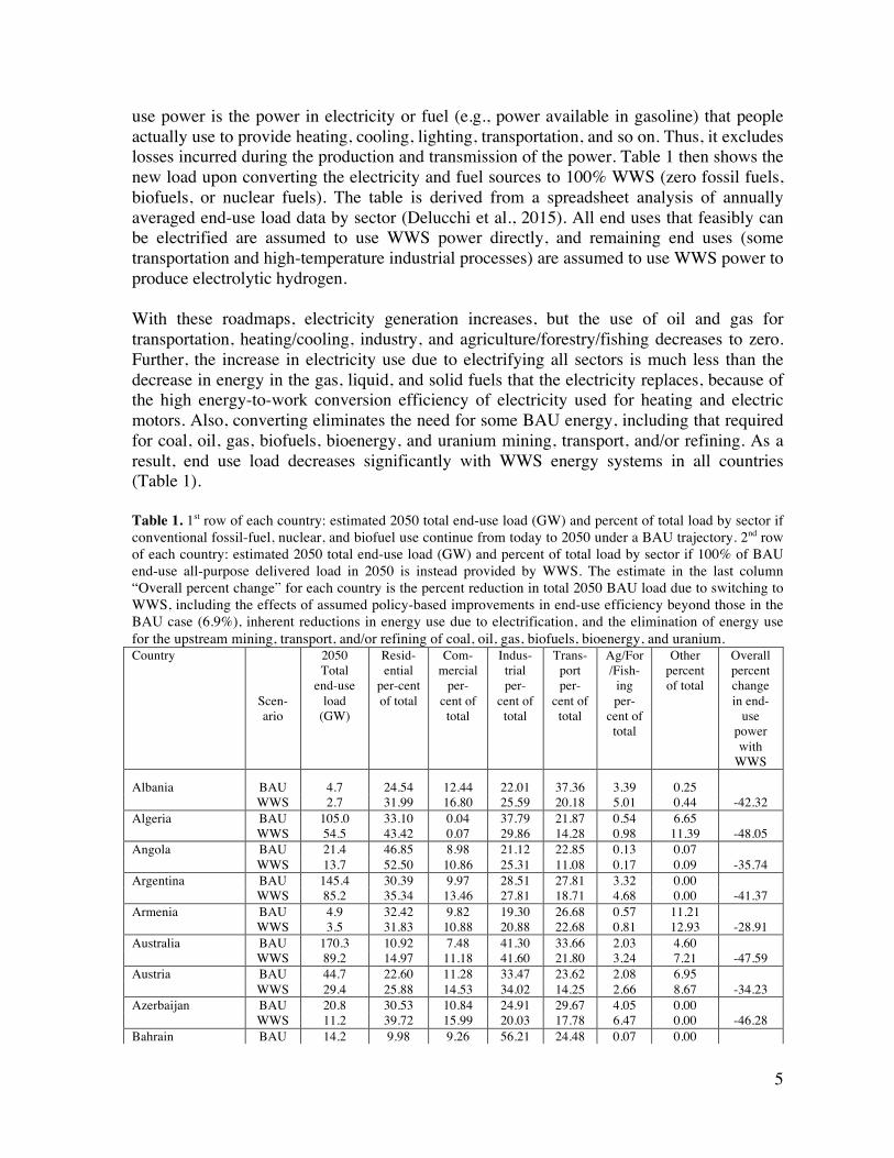
5

use power is the power in electricity or fuel (e.g., power available in gasoline) that people actually use to provide heating, cooling, lighting, transportation, and so on. Thus, it excludes losses incurred during the production and transmission of the power. Table 1 then shows the new load upon converting the electricity and fuel sources to 100% WWS (zero fossil fuels, biofuels, or nuclear fuels). The table is derived from a spreadsheet analysis of annually averaged end-use load data by sector (Delucchi et al., 2015). All end uses that feasibly can be electrified are assumed to use WWS power directly, and remaining end uses (some transportation and high-temperature industrial processes) are assumed to use WWS power to produce electrolytic hydrogen. With these roadmaps, electricity generation increases, but the use of oil and gas for transportation, heating/cooling, industry, and agriculture/forestry/fishing decreases to zero. Further, the increase in electricity use due to electrifying all sectors is much less than the decrease in energy in the gas, liquid, and solid fuels that the electricity replaces, because of the high energy-to-work conversion efficiency of electricity used for heating and electric motors. Also, converting eliminates the need for some BAU energy, including that required for coal, oil, gas, biofuels, bioenergy, and uranium mining, transport, and/or refining. As a result, end use load decreases significantly with WWS energy systems in all countries (Table 1). Table 1. 1st row of each country: estimated 2050 total end-use load (GW) and percent of total load by sector if conventional fossil-fuel, nuclear, and biofuel use continue from today to 2050 under a BAU trajectory. 2nd row of each country: estimated 2050 total end-use load (GW) and percent of total load by sector if 100% of BAU end-use all-purpose delivered load in 2050 is instead provided by WWS. The estimate in the last column “Overall percent change” for each country is the percent reduction in total 2050 BAU load due to switching to WWS, including the effects of assumed policy-based improvements in end-use efficiency beyond those in the BAU case (6.9%), inherent reductions in energy use due to electrification, and the elimination of energy use for the upstream mining, transport, and/or refining of coal, oil, gas, biofuels, bioenergy, and uranium. Country

Scen-ario

2050 Total

end-use load

(GW)

Resid-ential

per-cent of total

Com-mercial

per-cent of total

Indus-trial per-

cent of total

Trans-port per-

cent of total

Ag/For/Fish-

ing per-

cent of total

Other percent of total

Overall percent change in end-

use power with

WWS

Albania BAU 4.7 24.54 12.44 22.01 37.36 3.39 0.25 WWS 2.7 31.99 16.80 25.59 20.18 5.01 0.44 -42.32

Algeria BAU 105.0 33.10 0.04 37.79 21.87 0.54 6.65 WWS 54.5 43.42 0.07 29.86 14.28 0.98 11.39 -48.05

Angola BAU 21.4 46.85 8.98 21.12 22.85 0.13 0.07 WWS 13.7 52.50 10.86 25.31 11.08 0.17 0.09 -35.74

Argentina BAU 145.4 30.39 9.97 28.51 27.81 3.32 0.00 WWS 85.2 35.34 13.46 27.81 18.71 4.68 0.00 -41.37

Armenia BAU 4.9 32.42 9.82 19.30 26.68 0.57 11.21 WWS 3.5 31.83 10.88 20.88 22.68 0.81 12.93 -28.91

Australia BAU 170.3 10.92 7.48 41.30 33.66 2.03 4.60 WWS 89.2 14.97 11.18 41.60 21.80 3.24 7.21 -47.59

Austria BAU 44.7 22.60 11.28 33.47 23.62 2.08 6.95 WWS 29.4 25.88 14.53 34.02 14.25 2.66 8.67 -34.23

Azerbaijan BAU 20.8 30.53 10.84 24.91 29.67 4.05 0.00 WWS 11.2 39.72 15.99 20.03 17.78 6.47 0.00 -46.28

Bahrain BAU 14.2 9.98 9.26 56.21 24.48 0.07 0.00

6

WWS 6.5 16.66 15.72 50.76 16.70 0.16 0.00 -54.33 Bangladesh BAU 58.8 45.54 1.22 34.41 11.00 7.51 0.32

WWS 42.1 45.00 1.40 38.33 6.04 8.78 0.45 -28.49 Belarus BAU 56.0 19.66 12.45 29.15 16.75 3.97 18.02

WWS 39.3 23.12 15.72 26.39 8.76 4.95 21.05 -29.81 Belgium BAU 64.6 17.73 12.83 35.17 30.08 1.75 2.45

WWS 39.0 20.48 17.02 39.94 16.83 2.37 3.37 -39.58 Benin BAU 5.7 48.10 10.16 1.12 40.62 0.00 0.00

WWS 3.2 61.10 14.59 1.73 22.58 0.00 0.00 -43.95 Bolivia BAU 12.9 13.72 3.95 37.62 34.28 7.36 3.07

WWS 7.6 16.74 5.31 40.91 21.76 10.64 4.63 -41.42 Bosnia and BAU 7.7 24.32 0.00 30.03 31.64 0.24 13.77 Herzegovina WWS 4.6 31.16 0.00 30.38 17.04 0.41 21.00 -41.18 Botswana BAU 4.8 21.70 8.27 34.76 26.98 1.44 6.86

WWS 3.2 23.94 9.68 43.24 12.67 1.95 8.52 -33.69 Brazil BAU 627.5 9.63 9.13 49.78 26.73 4.52 0.21

WWS 389.7 11.53 11.42 52.50 18.01 6.25 0.28 -37.90 Brunei BAU 6.6 9.11 11.63 60.63 18.62 0.00 0.00 Darussalam WWS 2.2 20.01 26.53 36.39 17.07 0.00 0.00 -66.01 Bulgaria BAU 25.1 20.39 15.53 33.46 29.08 1.54 0.00

WWS 15.2 25.75 20.35 33.92 17.81 2.17 0.00 -39.40 Cambodia BAU 9.3 46.75 4.17 31.64 16.36 0.00 1.08

WWS 6.3 49.26 4.74 37.17 7.46 0.00 1.37 -31.68 Cameroon BAU 11.1 54.59 10.32 17.26 16.96 0.19 0.68

WWS 6.9 62.60 13.12 14.66 8.43 0.30 0.89 -37.36 Canada BAU 412.1 13.93 15.58 53.32 14.83 2.35 0.00

WWS 235.1 17.57 21.69 47.52 9.70 3.51 0.00 -42.95 Chile BAU 76.1 16.05 9.11 50.52 22.94 1.37 0.00

WWS 49.5 17.82 10.94 58.04 11.45 1.74 0.00 -35.02 China BAU 5,044.7 24.62 7.22 41.92 22.21 1.40 2.63

WWS 3,252.0 27.93 8.99 45.87 11.54 1.90 3.77 -35.54 Chinese Taipei BAU 170.0 11.87 9.45 55.37 18.95 1.16 3.20

WWS 111.6 13.47 11.22 59.79 9.15 1.57 4.79 -34.34 Colombia BAU 60.8 18.33 7.73 28.99 39.80 5.04 0.11

WWS 32.2 24.52 11.52 31.41 24.39 7.98 0.18 -47.00 Congo BAU 2.3 39.51 0.81 9.03 45.36 0.00 5.29

WWS 1.2 53.51 1.24 10.54 26.55 0.00 8.16 -46.79 Congo, Dem. BAU 42.4 56.80 0.25 39.57 3.04 0.00 0.34

Republic of WWS 31.1 54.89 0.26 43.18 1.29 0.00 0.38 -26.58 Costa Rica BAU 7.4 13.62 12.58 20.90 50.92 1.48 0.49

WWS 4.0 18.81 17.98 30.79 29.17 2.46 0.79 -45.61 Cote d'Ivoire BAU 12.2 58.09 12.09 15.36 12.18 2.27 0.00

WWS 8.3 61.70 14.20 15.76 5.59 2.75 0.00 -32.13 Croatia BAU 15.6 25.14 17.52 25.09 29.61 2.64 0.00

WWS 9.2 31.85 23.64 24.11 16.68 3.72 0.00 -41.30 Cuba BAU 14.5 15.45 5.01 59.07 13.91 1.71 4.85

WWS 10.2 16.37 5.54 63.86 6.46 2.09 5.68 -29.86 Cyprus BAU 4.7 14.76 18.16 7.58 56.99 1.79 0.72

WWS 2.4 21.43 27.48 11.03 35.66 3.07 1.33 -48.69 Czech Republic BAU 38.6 24.75 15.38 36.87 19.47 2.47 1.07

WWS 25.4 27.49 19.41 37.02 11.37 3.18 1.53 -34.25 Denmark BAU 24.3 29.20 15.59 22.34 26.91 5.90 0.07

WWS 15.7 37.52 20.91 19.14 14.49 7.86 0.09 -35.43 Dominican BAU 11.4 15.90 5.21 24.14 51.86 2.89 0.00

Republic WWS 6.2 21.52 7.48 35.85 29.91 5.24 0.00 -45.98 Ecuador BAU 24.0 11.31 4.52 26.03 55.66 0.73 1.74

WWS 10.8 18.29 7.81 30.32 38.69 1.34 3.55 -55.11 Egypt BAU 173.3 22.22 9.86 41.51 19.68 5.23 1.50

WWS 102.9 27.46 12.89 39.29 10.74 7.56 2.07 -40.64 El Salvador BAU 5.2 22.18 3.64 24.13 47.93 0.25 1.87

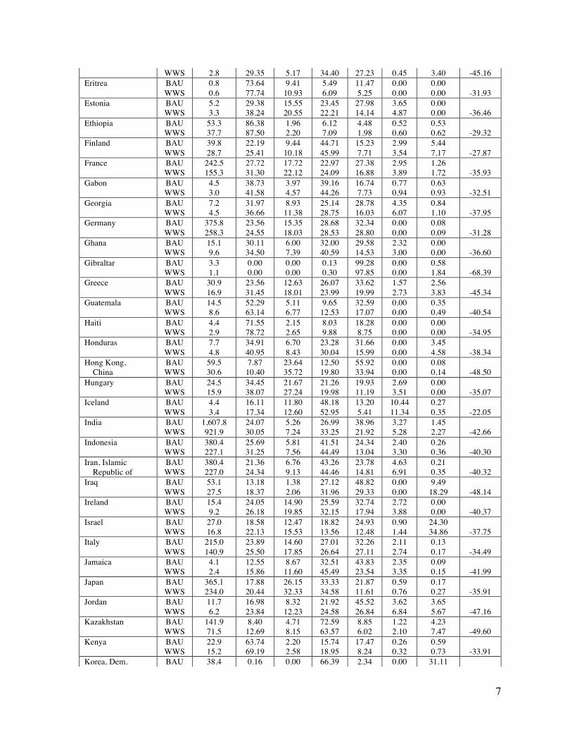
7

WWS 2.8 29.35 5.17 34.40 27.23 0.45 3.40 -45.16 Eritrea BAU 0.8 73.64 9.41 5.49 11.47 0.00 0.00

WWS 0.6 77.74 10.93 6.09 5.25 0.00 0.00 -31.93 Estonia BAU 5.2 29.38 15.55 23.45 27.98 3.65 0.00

WWS 3.3 38.24 20.55 22.21 14.14 4.87 0.00 -36.46 Ethiopia BAU 53.3 86.38 1.96 6.12 4.48 0.52 0.53

WWS 37.7 87.50 2.20 7.09 1.98 0.60 0.62 -29.32 Finland BAU 39.8 22.19 9.44 44.71 15.23 2.99 5.44

WWS 28.7 25.41 10.18 45.99 7.71 3.54 7.17 -27.87 France BAU 242.5 27.72 17.72 22.97 27.38 2.95 1.26

WWS 155.3 31.30 22.12 24.09 16.88 3.89 1.72 -35.93 Gabon BAU 4.5 38.73 3.97 39.16 16.74 0.77 0.63

WWS 3.0 41.58 4.57 44.26 7.73 0.94 0.93 -32.51 Georgia BAU 7.2 31.97 8.93 25.14 28.78 4.35 0.84

WWS 4.5 36.66 11.38 28.75 16.03 6.07 1.10 -37.95 Germany BAU 375.8 23.56 15.35 28.68 32.34 0.00 0.08

WWS 258.3 24.55 18.03 28.53 28.80 0.00 0.09 -31.28 Ghana BAU 15.1 30.11 6.00 32.00 29.58 2.32 0.00 WWS 9.6 34.50 7.39 40.59 14.53 3.00 0.00 -36.60 Gibraltar BAU 3.3 0.00 0.00 0.13 99.28 0.00 0.58 WWS 1.1 0.00 0.00 0.30 97.85 0.00 1.84 -68.39 Greece BAU 30.9 23.56 12.63 26.07 33.62 1.57 2.56 WWS 16.9 31.45 18.01 23.99 19.99 2.73 3.83 -45.34 Guatemala BAU 14.5 52.29 5.11 9.65 32.59 0.00 0.35 WWS 8.6 63.14 6.77 12.53 17.07 0.00 0.49 -40.54 Haiti BAU 4.4 71.55 2.15 8.03 18.28 0.00 0.00 WWS 2.9 78.72 2.65 9.88 8.75 0.00 0.00 -34.95 Honduras BAU 7.7 34.91 6.70 23.28 31.66 0.00 3.45 WWS 4.8 40.95 8.43 30.04 15.99 0.00 4.58 -38.34 Hong Kong, BAU 59.5 7.87 23.64 12.50 55.92 0.00 0.08

China WWS 30.6 10.40 35.72 19.80 33.94 0.00 0.14 -48.50 Hungary BAU 24.5 34.45 21.67 21.26 19.93 2.69 0.00 WWS 15.9 38.07 27.24 19.98 11.19 3.51 0.00 -35.07 Iceland BAU 4.4 16.11 11.80 48.18 13.20 10.44 0.27 WWS 3.4 17.34 12.60 52.95 5.41 11.34 0.35 -22.05 India BAU 1,607.8 24.07 5.26 26.99 38.96 3.27 1.45 WWS 921.9 30.05 7.24 33.25 21.92 5.28 2.27 -42.66 Indonesia BAU 380.4 25.69 5.81 41.51 24.34 2.40 0.26 WWS 227.1 31.25 7.56 44.49 13.04 3.30 0.36 -40.30 Iran, Islamic BAU 380.4 21.36 6.76 43.26 23.78 4.63 0.21

Republic of WWS 227.0 24.34 9.13 44.46 14.81 6.91 0.35 -40.32 Iraq BAU 53.1 13.18 1.38 27.12 48.82 0.00 9.49 WWS 27.5 18.37 2.06 31.96 29.33 0.00 18.29 -48.14 Ireland BAU 15.4 24.05 14.90 25.59 32.74 2.72 0.00 WWS 9.2 26.18 19.85 32.15 17.94 3.88 0.00 -40.37 Israel BAU 27.0 18.58 12.47 18.82 24.93 0.90 24.30 WWS 16.8 22.13 15.53 13.56 12.48 1.44 34.86 -37.75 Italy BAU 215.0 23.89 14.60 27.01 32.26 2.11 0.13 WWS 140.9 25.50 17.85 26.64 27.11 2.74 0.17 -34.49 Jamaica BAU 4.1 12.55 8.67 32.51 43.83 2.35 0.09 WWS 2.4 15.86 11.60 45.49 23.54 3.35 0.15 -41.99 Japan BAU 365.1 17.88 26.15 33.33 21.87 0.59 0.17 WWS 234.0 20.44 32.33 34.58 11.61 0.76 0.27 -35.91 Jordan BAU 11.7 16.98 8.32 21.92 45.52 3.62 3.65 WWS 6.2 23.84 12.23 24.58 26.84 6.84 5.67 -47.16 Kazakhstan BAU 141.9 8.40 4.71 72.59 8.85 1.22 4.23 WWS 71.5 12.69 8.15 63.57 6.02 2.10 7.47 -49.60 Kenya BAU 22.9 63.74 2.20 15.74 17.47 0.26 0.59 WWS 15.2 69.19 2.58 18.95 8.24 0.32 0.73 -33.91 Korea, Dem. BAU 38.4 0.16 0.00 66.39 2.34 0.00 31.11

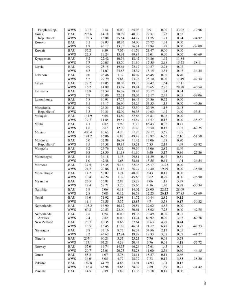
8

People's Rep. WWS 30.7 0.14 0.00 65.93 0.91 0.00 33.02 -19.96 Korea, BAU 295.6 14.18 20.92 40.70 22.31 1.23 0.67

Republic of WWS 192.3 15.88 25.54 44.27 11.75 1.71 0.84 -34.92 Kosovo BAU 3.1 38.03 10.93 24.00 25.72 1.31 0.00 WWS 1.9 45.17 13.75 26.24 12.94 1.89 0.00 -38.09 Kuwait BAU 57.2 9.89 7.05 61.59 21.47 0.00 0.00 WWS 22.5 19.24 13.91 49.84 17.01 0.00 0.00 -60.69 Kyrgyzstan BAU 9.2 22.42 10.54 18.42 34.86 1.92 11.84 WWS 5.7 29.05 13.70 21.30 17.55 2.68 15.72 -38.11 Latvia BAU 9.9 25.15 19.64 22.17 30.27 2.74 0.02 WWS 6.5 31.07 24.83 25.39 15.15 3.54 0.02 -34.35 Lebanon BAU 9.0 23.46 7.32 16.07 46.45 0.00 6.70 WWS 5.2 29.79 9.85 23.76 25.10 0.00 11.49 -42.34 Libya BAU 27.2 12.05 10.02 19.75 39.42 1.64 17.11 WWS 16.2 14.89 13.07 19.84 20.65 2.76 28.78 -40.54 Lithuania BAU 12.9 22.54 16.08 29.43 30.17 1.74 0.04 WWS 7.9 30.06 22.21 28.05 17.17 2.45 0.05 -39.06 Luxembourg BAU 5.8 10.91 17.55 16.45 54.36 0.72 0.00 WWS 3.1 14.17 26.90 24.24 33.55 1.15 0.00 -46.56 Macedonia, BAU 4.9 26.21 15.24 32.50 22.49 1.13 2.43

Republic of WWS 3.3 30.31 18.09 36.55 10.63 1.42 3.00 -33.51 Malaysia BAU 141.9 8.65 13.80 52.66 24.81 0.08 0.00 WWS 77.7 11.85 19.57 53.87 14.57 0.15 0.00 -45.27 Malta BAU 4.1 4.82 5.99 3.30 85.43 0.06 0.41 WWS 1.6 9.67 12.30 6.32 70.50 0.15 1.05 -62.25 Mexico BAU 400.4 10.65 4.25 51.23 29.17 3.65 1.05 WWS 194.2 16.06 6.82 49.48 18.97 6.52 2.16 -51.50 Moldova, BAU 5.0 32.88 16.07 31.42 17.06 1.78 0.80

Republic of WWS 3.5 34.58 19.14 35.21 7.83 2.14 1.09 -29.82 Mongolia BAU 9.2 25.76 8.32 39.56 15.06 2.82 8.49 WWS 6.8 28.30 11.18 41.10 6.40 3.17 9.86 -25.86 Montenegro BAU 1.6 36.18 1.35 29.81 31.39 0.47 0.81 WWS 1.0 42.48 1.68 38.61 15.55 0.64 1.04 -36.54 Morocco BAU 37.5 18.35 9.16 32.38 25.17 14.93 0.00 WWS 24.2 20.86 11.18 36.27 12.40 19.29 0.00 -35.50 Mozambique BAU 14.2 50.07 1.24 40.08 8.43 0.18 0.00 WWS 10.4 49.24 1.32 45.63 3.62 0.20 0.00 -26.90 Myanmar BAU 26.5 56.81 2.87 25.29 8.06 1.19 5.79 WWS 18.4 58.71 3.20 25.65 4.16 1.40 6.88 -30.34 Namibia BAU 3.9 7.06 0.11 14.02 28.00 22.72 28.09 WWS 2.8 7.08 0.12 16.59 12.23 26.13 37.85 -28.69 Nepal BAU 16.0 71.92 2.98 11.72 10.44 2.82 0.12 WWS 11.1 74.55 3.37 13.83 4.71 3.38 0.17 -30.82 Netherlands BAU 105.2 16.90 16.12 29.54 32.62 4.83 0.00 WWS 60.2 20.53 23.00 30.61 18.62 7.25 0.00 -42.75 Netherlands BAU 7.8 1.24 0.00 19.36 78.49 0.00 0.91

Antilles WWS 2.4 2.82 0.00 13.24 80.92 0.00 3.02 -69.78 New Zealand BAU 23.7 10.35 8.66 37.64 38.63 4.28 0.44 WWS 13.5 13.45 11.88 46.31 21.12 6.48 0.77 -42.73 Nicaragua BAU 3.8 37.16 9.72 16.37 34.56 2.13 0.05 WWS 2.2 45.62 12.94 19.97 18.33 3.08 0.07 -41.27 Nigeria BAU 207.1 60.21 3.53 25.21 7.76 0.01 3.28 WWS 133.1 67.21 4.39 20.44 3.76 0.01 4.18 -35.72 Norway BAU 37.0 19.74 14.55 46.24 17.61 1.45 0.41 WWS 20.7 27.01 20.75 38.28 11.00 2.36 0.60 -44.15 Oman BAU 55.2 4.07 3.78 74.11 15.27 0.11 2.66 WWS 34.0 5.05 4.77 78.72 7.73 0.17 3.55 -38.50 Pakistan BAU 169.8 44.79 4.88 33.91 14.93 1.31 0.17 WWS 116.4 45.98 5.65 38.39 7.89 1.89 0.21 -31.42 Panama BAU 14.5 7.39 7.89 11.36 73.18 0.17 0.00

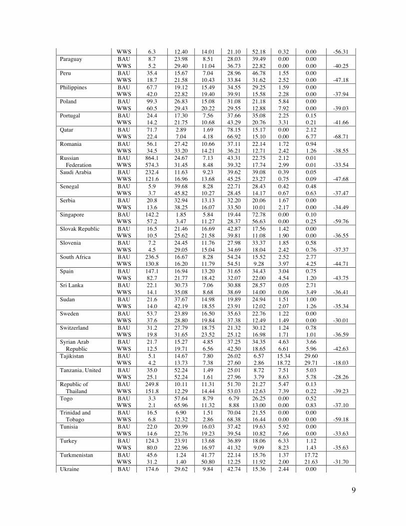
9

WWS 6.3 12.40 14.01 21.10 52.18 0.32 0.00 -56.31 Paraguay BAU 8.7 23.98 8.51 28.03 39.49 0.00 0.00 WWS 5.2 29.40 11.04 36.73 22.82 0.00 0.00 -40.25 Peru BAU 35.4 15.67 7.04 28.96 46.78 1.55 0.00 WWS 18.7 21.58 10.43 33.84 31.62 2.52 0.00 -47.18 Philippines BAU 67.7 19.12 15.49 34.55 29.25 1.59 0.00 WWS 42.0 22.82 19.40 39.91 15.58 2.28 0.00 -37.94 Poland BAU 99.3 26.83 15.08 31.08 21.18 5.84 0.00 WWS 60.5 29.43 20.22 29.55 12.88 7.92 0.00 -39.03 Portugal BAU 24.4 17.30 7.56 37.66 35.08 2.25 0.15 WWS 14.2 21.75 10.68 43.29 20.76 3.31 0.21 -41.66 Qatar BAU 71.7 2.89 1.69 78.15 15.17 0.00 2.12 WWS 22.4 7.04 4.18 66.92 15.10 0.00 6.77 -68.71 Romania BAU 56.1 27.42 10.66 37.11 22.14 1.72 0.94 WWS 34.5 33.20 14.21 36.21 12.71 2.42 1.26 -38.55 Russian BAU 864.1 24.67 7.13 43.31 22.75 2.12 0.01

Federation WWS 574.3 31.45 8.48 39.32 17.74 2.99 0.01 -33.54 Saudi Arabia BAU 232.4 11.63 9.23 39.62 39.08 0.39 0.05 WWS 121.6 16.96 13.68 45.25 23.27 0.75 0.09 -47.68 Senegal BAU 5.9 39.68 8.28 22.71 28.43 0.42 0.48 WWS 3.7 45.82 10.27 28.45 14.17 0.67 0.63 -37.47 Serbia BAU 20.8 32.94 13.13 32.20 20.06 1.67 0.00 WWS 13.6 38.25 16.07 33.50 10.01 2.17 0.00 -34.49 Singapore BAU 142.2 1.85 5.84 19.44 72.78 0.00 0.10 WWS 57.2 3.47 11.27 28.37 56.63 0.00 0.25 -59.76 Slovak Republic BAU 16.5 21.46 16.69 42.87 17.56 1.42 0.00 WWS 10.5 25.62 21.58 39.81 11.08 1.90 0.00 -36.55 Slovenia BAU 7.2 24.45 11.76 27.98 33.37 1.85 0.58 WWS 4.5 29.05 15.04 34.69 18.04 2.42 0.76 -37.37 South Africa BAU 236.5 16.67 8.28 54.24 15.52 2.52 2.77 WWS 130.8 16.20 11.79 54.51 9.28 3.97 4.25 -44.71 Spain BAU 147.1 16.94 13.20 31.65 34.43 3.04 0.75 WWS 82.7 21.77 18.42 32.07 22.00 4.54 1.20 -43.75 Sri Lanka BAU 22.1 30.73 7.06 30.88 28.57 0.05 2.71 WWS 14.1 35.08 8.68 38.69 14.00 0.06 3.49 -36.41 Sudan BAU 21.6 37.67 14.98 19.89 24.94 1.51 1.00 WWS 14.0 42.19 18.55 23.91 12.02 2.07 1.26 -35.34 Sweden BAU 53.7 23.89 16.50 35.63 22.76 1.22 0.00 WWS 37.6 28.80 19.84 37.38 12.49 1.49 0.00 -30.01 Switzerland BAU 31.2 27.79 18.75 21.32 30.12 1.24 0.78 WWS 19.8 31.65 23.52 25.12 16.98 1.71 1.01 -36.59 Syrian Arab BAU 21.7 15.27 4.85 37.25 34.35 4.63 3.66

Republic WWS 12.5 19.71 6.56 42.50 18.65 6.61 5.96 -42.63 Tajikistan BAU 5.1 14.67 7.80 26.02 6.57 15.34 29.60 WWS 4.2 13.73 7.38 27.60 2.86 18.72 29.71 -18.03 Tanzania, United BAU 35.0 52.24 1.49 25.01 8.72 7.51 5.03 WWS 25.1 52.24 1.61 27.96 3.79 8.63 5.78 -28.26 Republic of BAU 249.8 10.11 11.31 51.70 21.27 5.47 0.13

Thailand WWS 151.8 12.29 14.44 53.03 12.63 7.39 0.22 -39.23 Togo BAU 3.3 57.64 8.79 6.79 26.25 0.00 0.52 WWS 2.1 65.96 11.32 8.88 13.00 0.00 0.83 -37.10 Trinidad and BAU 16.5 6.90 1.51 70.04 21.55 0.00 0.00

Tobago WWS 6.8 12.32 2.86 68.38 16.44 0.00 0.00 -59.18 Tunisia BAU 22.0 20.99 16.03 37.42 19.63 5.92 0.00 WWS 14.6 22.76 19.23 39.54 10.82 7.66 0.00 -33.63 Turkey BAU 124.3 23.91 13.68 36.89 18.06 6.33 1.12 WWS 80.0 22.96 16.97 41.32 9.09 8.23 1.43 -35.63 Turkmenistan BAU 45.6 1.24 41.77 22.14 15.76 1.37 17.72 WWS 31.2 1.40 50.80 12.25 11.92 2.00 21.63 -31.70 Ukraine BAU 174.6 29.62 9.84 42.74 15.36 2.44 0.00

10

WWS 119.1 32.28 12.47 42.43 9.66 3.16 0.00 -31.81 United Arab BAU 176.0 4.14 5.46 56.07 32.78 0.00 1.56

Emirates WWS 110.7 5.04 6.73 69.55 16.23 0.00 2.45 -37.11 United Kingdom BAU 225.1 29.88 14.15 25.92 28.60 0.60 0.85 WWS 127.9 36.22 19.98 24.95 16.70 0.94 1.22 -43.18 United States of BAU 2,310.3 16.44 14.83 28.24 38.42 1.25 0.82

America WWS 1,296.4 21.33 21.02 28.22 26.10 1.88 1.45 -43.89 Uruguay BAU 8.0 16.22 11.11 30.33 40.49 1.66 0.18 WWS 4.7 20.79 14.95 38.86 22.54 2.55 0.31 -42.00 Uzbekistan BAU 81.6 39.42 11.10 28.09 8.54 4.99 7.86 WWS 57.7 37.29 12.93 25.90 6.39 6.69 10.80 -29.38 Venezuela BAU 121.9 8.87 6.05 50.76 34.27 0.06 0.00 WWS 61.6 12.59 9.36 56.75 21.17 0.12 0.00 -49.44 Vietnam BAU 133.1 23.66 5.23 50.07 19.24 1.80 0.00 WWS 91.6 23.60 5.97 59.51 8.71 2.21 0.00 -31.18 Yemen BAU 12.8 9.39 1.37 27.37 33.32 19.55 9.00 WWS 7.5 11.64 1.81 28.25 17.77 27.44 13.08 -41.59 Zambia BAU 14.0 52.30 2.60 38.82 4.48 1.07 0.73 WWS 10.4 51.11 2.72 42.07 1.93 1.29 0.88 -25.95 Zimbabwe BAU 17.2 50.91 7.95 18.21 4.58 16.99 1.35 WWS 12.7 49.75 8.58 19.17 1.88 19.09 1.53 -26.14 All countries BAU 19,399.8 21.64 9.66 37.97 27.01 2.06 1.66

WWS 11,796.7 25.90 12.66 39.96 16.06 2.96 2.47 -39.19 BAU values are extrapolated from IEA (2015) data for 2012 to 2050 as follows: EIA’s International Energy Outlook (IEO) projects energy use by end-use sector, fuel, and world region out to 2040 (EIA, 2015). This was extended to 2075 using a ten-year moving linear extrapolation. EIA sectors and fuels were then mapped to IEA sectors and fuels, and each country’s 2012 energy consumption by sector and fuel was scaled by the ratio of EIA’s 2050/2012 energy consumption by sector and fuel for each region. The transportation load includes, among other loads, energy produced in each country for international transportation and shipping. 2050 WWS values are estimated from 2050 BAU values assuming electrification of end-uses and effects of additional energy-efficiency measures. See Delucchi et al. (2015) for details. In 2012, the 139-country all-purpose, end-use load was ~11.95 TW (terawatts, or trillion watts). Of this, 2.4 TW (20.1%) was electric power load. If the countries follow the BAU trajectory, which involves increasing load, modest shifts in the power sector away from coal toward natural gas, biofuels, bioenergy and some WWS, and modest end-use energy efficiency improvements, their summed all-purpose end-use load is expected to grow to 19.4 TW in 2050 (Table 1).

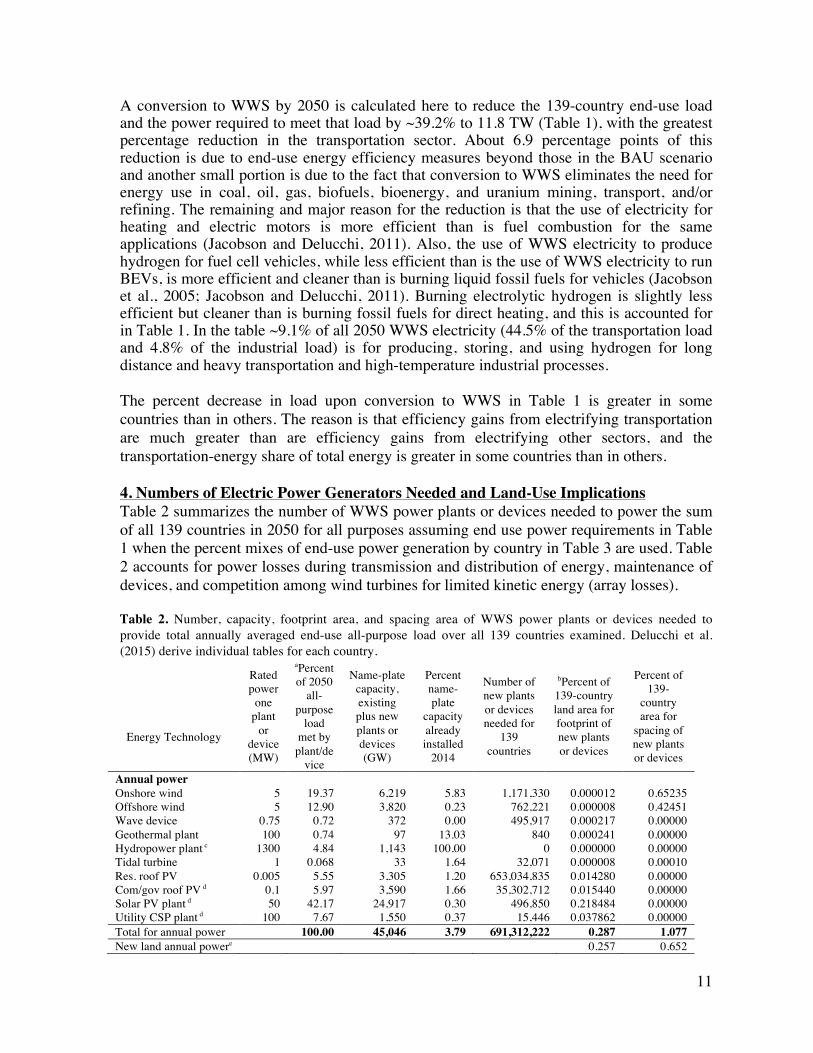
11

A conversion to WWS by 2050 is calculated here to reduce the 139-country end-use load and the power required to meet that load by ~39.2% to 11.8 TW (Table 1), with the greatest percentage reduction in the transportation sector. About 6.9 percentage points of this reduction is due to end-use energy efficiency measures beyond those in the BAU scenario and another small portion is due to the fact that conversion to WWS eliminates the need for energy use in coal, oil, gas, biofuels, bioenergy, and uranium mining, transport, and/or refining. The remaining and major reason for the reduction is that the use of electricity for heating and electric motors is more efficient than is fuel combustion for the same applications (Jacobson and Delucchi, 2011). Also, the use of WWS electricity to produce hydrogen for fuel cell vehicles, while less efficient than is the use of WWS electricity to run BEVs, is more efficient and cleaner than is burning liquid fossil fuels for vehicles (Jacobson et al., 2005; Jacobson and Delucchi, 2011). Burning electrolytic hydrogen is slightly less efficient but cleaner than is burning fossil fuels for direct heating, and this is accounted for in Table 1. In the table ~9.1% of all 2050 WWS electricity (44.5% of the transportation load and 4.8% of the industrial load) is for producing, storing, and using hydrogen for long distance and heavy transportation and high-temperature industrial processes. The percent decrease in load upon conversion to WWS in Table 1 is greater in some countries than in others. The reason is that efficiency gains from electrifying transportation are much greater than are efficiency gains from electrifying other sectors, and the transportation-energy share of total energy is greater in some countries than in others. 4. Numbers of Electric Power Generators Needed and Land-Use Implications Table 2 summarizes the number of WWS power plants or devices needed to power the sum of all 139 countries in 2050 for all purposes assuming end use power requirements in Table 1 when the percent mixes of end-use power generation by country in Table 3 are used. Table 2 accounts for power losses during transmission and distribution of energy, maintenance of devices, and competition among wind turbines for limited kinetic energy (array losses). Table 2. Number, capacity, footprint area, and spacing area of WWS power plants or devices needed to provide total annually averaged end-use all-purpose load over all 139 countries examined. Delucchi et al. (2015) derive individual tables for each country.

Energy Technology

Rated power

one plant

or device (MW)

aPercent of 2050

all-purpose

load met by plant/de

vice

Name-plate capacity, existing plus new plants or devices (GW)

Percent name-plate

capacity already installed

2014

Number of new plants or devices needed for

139 countries

bPercent of 139-country land area for footprint of new plants or devices

Percent of 139-

country area for

spacing of new plants or devices

Annual power Onshore wind 5 19.37 6,219 5.83 1,171,330 0.000012 0.65235 Offshore wind 5 12.90 3,820 0.23 762,221 0.000008 0.42451 Wave device 0.75 0.72 372 0.00 495,917 0.000217 0.00000 Geothermal plant 100 0.74 97 13.03 840 0.000241 0.00000 Hydropower plant c 1300 4.84 1,143 100.00 0 0.000000 0.00000 Tidal turbine 1 0.068 33 1.64 32,071 0.000008 0.00010 Res. roof PV 0.005 5.55 3,305 1.20 653,034,835 0.014280 0.00000 Com/gov roof PV d 0.1 5.97 3,590 1.66 35,302,712 0.015440 0.00000 Solar PV plant d 50 42.17 24,917 0.30 496,850 0.218484 0.00000 Utility CSP plant d 100 7.67 1,550 0.37 15,446 0.037862 0.00000 Total for annual power 100.00 45,046 3.79 691,312,222 0.287 1.077 New land annual powere 0.257 0.652

12

For peaking/storage Additional CSP f 100 4.60% 930 0.00 9,302 0.022801 0.000 Solar thermal f 50 5,004 0.64 99,436 0.005932 0.000 Geothermal heat f 50 70 100.00 0 0.000000 0.000 Total all 51,050 3.54 691,420,960 0.315 1.077 Total new lande 0.285 0.652 The total number of each device is the sum among all countries. The number of devices in each country is the end use load in 2050 in each country to be supplied by WWS (Table 1) multiplied by the fraction of load satisfied by each WWS device in each country (Table 3) and divided by the annual power output from each device. The annual output by device equals the rated power (this table; same for all countries) multiplied by the country-specific annual capacity factor of the device, diminished by transmission, distribution, maintenance, and array losses. The capacity factors, given in Delucchi et al. (2015), before transmission, distribution, and maintenance losses for onshore and offshore wind turbines at 100-m hub height in 2050, are calculated country by country from global model simulations of winds and wind power (Figure 3), accounting for competition among wind turbines for available kinetic energy based on the approximate number of turbines needed per country as determined iteratively from Tables 2 and 3. Wind array losses due to competition among turbines for the same energy are calculated here to be ~8.5%. The 2050 139-country mean onshore wind capacity factor calculated in this manner after transmission, distribution, maintenance, and array losses is 37.0%. That for offshore wind is ~40.1%. Short- and moderate distance transmission, distribution, and maintenance losses for all energy sources treated here, except rooftop PV, are assumed to be 5-10%. Rooftop PV losses are assumed to be 1-2%. The plans assume 38 (30-45)% of onshore wind and solar and 20 (15-25)% of offshore wind is subject to long-distance transmission with line lengths of 1400 (1200-1600) km and 120 (80-160) km, respectively. Line losses are 4 (3-5)% per 1000 km plus 1.5 (1.3-1.8)% of power in the station equipment. Footprint and spacing areas are calculated from the spreadsheets in Delucchi et al. (2015). Footprint is the area on the top surface of soil covered by an energy technology, thus does not include underground structures. aTotal end-use power demand in 2050 with 100% WWS is estimated from Table 1. bTotal land area for each country is given in Delucchi et al. (2015). 139-country land area is 119,725,384 km2.

The world land area is 510,072,000 km2. cThe average capacity factors of hydropower plants are assumed to increase from their current values to 50.0%,

except for Tajikistan and Paraguay, which are assumed to increase to 40% (see text). dThe solar PV panels used for this calculation are Sun Power E20 panels. CSP plant characteristics are

patterned after the Ivanpah facility but assuming storage, namely a maximum charge to discharge rate (storage size to generator size ratio) of 2.62:1. The capacity factors used for residential PV, commercial/government rooftop PV, utility scale PV, and CSP are calculated here country-by-country with the 3-D global model simulations also used to calculate solar resource analysis (Figure 5), and are given in Delucchi et al. (2015). For utility solar PV plants, nominal “spacing” between panels is included in the plant footprint area.

eThe footprint area requiring new land equals the sum of the footprint areas for new onshore wind, geothermal, hydropower, and utility solar PV. Offshore wind, wave and tidal are in water so do not require new land. Similarly, rooftop solar PV does not use new land because the rooftops already exist. Only onshore wind requires new land for spacing area. Spacing area is for onshore and offshore wind is calculated as 42D2, where D=rotor diameter. The 5-MW Senvion (RePower) turbine assumed has D=126 m.

The other energy sources either are in water or on rooftops, or do not use new land for spacing. Note that the spacing area for onshore wind can be used for multiple purposes, such as open space, agriculture, grazing, etc.

fThe installed capacities for peaking power/storage are estimated based on data from Jacobson et al. (2015b). Additional CSP is CSP plus storage beyond that needed for annual power generation to firm the grid across all countries. Additional solar thermal and geothermal are used for soil heat storage. Other types of storage are also used in Jacobson et al. (2015b).

Rooftop PV in Table 2 is divided into residential (5-kW systems on average) and commercial/government (100-kW systems on average). Rooftop PV can be placed on

13

existing rooftops or on elevated canopies above parking lots, highways, and structures without taking up additional undeveloped land. Table 4 summarizes projected 2050 rooftop areas by country usable for solar PV on residential and commercial/government buildings, carports, garages, parking structures, and parking lot canopies. The rooftop areas in Table 4 are used to calculate potential rooftop generation, which in turn limits the penetration of PV on residential and commercial/government buildings in Table 3. Utility-scale PV power plants are sized, on average, relatively small (50 MW) to allow them to be placed optimally in available locations. While utility-scale PV can operate in any country because it can take advantage of both direct and diffuse solar radiation, CSP is assumed to be viable only in countries with significant direct solar radiation, and its penetration in each country is limited to less than its technical potential. Onshore wind is available to some extent in every country but assumed to be viable in high penetrations primarily in countries with good wind resources (Section 5.1). Offshore wind is assumed to be viable in any country with either ocean or lake coastline (Section 5.1). Wind and solar are the only two sources of electric power with sufficient resource to power the world independently on their own. Averaged over the 139 countries, wind (~32.3%) and solar (61.4%) are the largest generators of annually averaged end-use electric power under these plans. The ratio of wind to solar end-use power is 0.53:1. Under the roadmaps, the 2050 nameplate capacity of hydropower in each country is assumed to be exactly the same as in 2014. However, existing dams in most countries are assumed to run more efficiently for producing peaking power, thus the capacity factor of dams is assumed to increase (Section 5.4). Geothermal, tidal, and wave energy expansions are limited in each country by their technical potentials (Sections 5.3 and 5.5). Table 2 indicates that 3.8% of the summed nameplate capacity required for a 100% WWS system for 2050 all-purpose energy in the 139 countries is already installed as of the end of 2014. Figure 1 shows that the countries closest to 100% 2050 all-purpose WWS power as of the end of 2014 are Norway (67%), Paraguay (54%), and Iceland (39%), Tajikistan (34%), Portugal (26%), Sweden (21%), and Switzerland (20.6%). The United States (4.2%) ranks 56th and China (3.4%) ranks 65th. Figure 1. Countries ranked in order of how close they are at the end of 2014 to reaching 100% WWS power for all purposes in 2050. The percentages are of 2050 WWS installed capacity (summed over all WWS technologies) needed that are already installed..

14

15

Table 2 also lists 1) installed capacities beyond those needed to match annually averaged power demand for CSP with storage, 2) solar thermal for current and stored heat, and 3) geothermal for current and stored heat. These additional capacities are estimated using data from the grid integration study of Jacobson et al. (2015b) and are needed to produce peaking power, to account for additional loads due to losses in and out of storage, and to ensure reliability of the grid, as described and quantified in that paper (see also Section 6). Table 3. Percent of annually-averaged 2050 country-specific all-purpose end-use load (not installed capacity) in a WWS world from Table 1 proposed here to be met by the given electric power generator. All rows add up to 100%.

Country On-shore wind

Off-shore wind

Wave Geoth-ermal

Hydro-electric

Tidal Res PV

Comm/gov PV

Utility PV

CSP

Albania 1.50 0.28 2.00 0.00 35.10 0.45 7.54 9.59 43.54 0.00 Algeria 1.25 0.00 0.92 0.00 0.25 0.02 9.33 10.33 62.90 15.00 Angola 8.00 1.70 3.00 0.00 3.64 0.09 36.92 27.57 8.58 10.50 Argentina 30.00 20.00 2.80 1.07 7.27 0.01 8.04 9.22 11.59 10.00 Armenia 18.50 0.00 0.00 0.64 16.96 0.00 5.09 5.46 33.35 20.00 Australia 30.00 6.20 5.00 0.40 4.93 0.14 4.83 5.98 32.53 10.00 Austria 27.00 0.00 0.00 0.00 22.68 0.00 5.12 5.55 39.45 0.20 Azerbaijan 45.00 0.00 0.00 0.00 4.42 0.00 6.91 8.89 27.78 7.00 Bahrain 1.00 8.00 1.25 0.00 0.00 0.19 3.32 5.41 60.83 20.00 Bangladesh 15.00 0.00 0.65 0.00 0.27 0.09 16.55 6.59 55.85 5.00 Belarus 45.00 0.00 0.00 0.02 0.01 0.00 0.77 1.43 51.77 1.00 Belgium 8.00 18.00 0.08 0.00 1.83 0.03 4.56 4.75 62.75 0.00 Benin 29.20 0.30 0.50 0.00 0.02 0.38 11.96 5.81 41.83 10.00 Bolivia 25.00 0.00 0.00 14.98 3.17 0.00 20.12 8.61 23.12 5.00 Bosnia and Herzegovina 10.50 1.20 0.22 0.00 21.86 0.27 6.85 9.43 44.67 5.00 Botswana 30.00 0.00 0.00 0.00 0.00 0.00 5.53 8.61 40.85 15.00 Brazil 0.85 17.00 0.97 0.00 11.31 0.01 7.40 10.21 42.24 10.00 Brunei Darussalam 5.00 11.50 0.00 0.00 0.00 0.00 7.00 8.78 57.72 10.00 Bulgaria 7.00 0.00 0.00 0.00 12.23 0.08 1.56 4.40 74.72 0.00 Cambodia 30.00 7.90 2.00 0.00 2.68 0.19 26.02 12.15 14.05 5.00 Cameroon 15.00 1.50 1.00 0.00 5.19 0.18 10.03 5.47 46.63 15.00 Canada 37.50 21.00 2.00 1.91 16.24 0.21 1.46 1.69 17.99 0.00 Chile 25.00 10.00 1.00 3.15 6.67 0.05 5.33 6.92 36.89 5.00 China 16.00 12.90 0.20 0.05 4.33 0.02 3.65 4.52 49.34 9.00 Chinese Taipei 2.00 38.00 0.70 27.14 2.08 0.01 1.48 3.11 25.48 0.00 Colombia 25.00 14.10 1.00 0.00 14.43 0.38 9.38 6.26 24.45 5.00 Congo 10.00 12.00 1.90 0.00 4.90 1.01 27.71 21.61 20.88 0.00 Congo, Dem. Republic 10.00 0.00 0.00 0.00 0.11 0.04 6.75 1.73 56.37 25.00 Costa Rica 3.00 1.10 1.00 26.68 21.71 0.31 17.05 17.39 6.76 5.00 Cote d'Ivoire 22.40 7.00 2.50 0.00 3.62 0.15 11.23 7.09 45.91 0.10 Croatia 30.00 0.00 1.00 0.00 11.74 0.13 2.41 4.84 48.87 1.00 Cuba 22.93 15.00 2.00 0.00 0.29 0.12 13.34 8.40 32.92 5.00 Cyprus 20.00 13.00 1.00 0.00 0.00 0.51 13.02 14.06 28.41 10.00 Czech Republic 25.00 0.00 0.00 0.00 4.39 0.00 4.14 6.64 59.84 0.00 Denmark 28.00 57.00 3.00 0.00 0.03 0.08 1.59 1.64 8.66 0.00 Dominican Republic 25.00 5.00 2.00 9.94 4.63 0.20 24.12 20.01 4.11 5.00 Ecuador 35.00 1.00 2.00 0.33 10.20 0.57 25.22 13.89 11.79 0.00 Egypt 20.00 0.25 1.00 0.00 1.36 0.01 11.72 8.07 42.58 15.00 El Salvador 10.00 2.00 3.00 32.07 8.25 0.43 17.79 10.09 11.37 5.00 Eritrea 15.00 5.00 2.00 0.00 0.00 2.19 52.53 17.26 1.02 5.00 Estonia 60.00 20.66 2.00 0.00 0.12 0.37 0.78 1.29 14.77 0.00 Ethiopia 16.00 0.00 0.00 4.08 2.51 0.00 17.74 5.12 36.55 18.00 Finland 32.00 41.00 1.50 0.00 5.57 0.04 0.25 0.56 19.09 0.00 France 30.00 25.00 1.25 0.02 8.17 0.16 10.36 9.71 14.59 0.75

16

Gabon 15.00 20.00 2.00 0.00 2.82 0.41 5.97 7.33 46.47 0.00 Georgia 18.00 4.00 2.00 0.00 30.01 0.28 5.21 7.30 33.21 0.00 Germany 18.00 17.00 0.35 0.01 2.20 0.00 5.72 5.49 51.23 0.00 Ghana 21.10 4.00 1.00 0.00 8.25 0.13 8.87 6.34 50.07 0.25 Gibraltar 0.03 35.00 0.50 0.00 0.00 1.17 0.37 0.75 62.15 0.04 Greece 30.00 4.00 1.00 2.40 10.05 0.07 14.19 9.14 24.45 4.70 Guatemala 7.00 3.00 1.00 23.68 5.82 0.14 22.54 10.38 16.43 10.00 Haiti 30.00 11.00 1.00 0.00 1.05 0.43 28.58 6.32 11.61 10.00 Honduras 25.00 7.50 4.00 11.17 5.78 0.26 17.22 6.65 14.92 7.50 Hong Kong, China 0.25 35.00 1.20 0.00 0.00 0.04 3.18 3.71 41.62 15.00 Hungary 1.70 0.00 0.00 2.15 0.18 0.00 3.01 4.37 88.59 0.00 Iceland 39.03 6.00 2.00 23.56 29.05 0.36 0.00 0.00 0.00 0.00 India 17.00 3.20 0.38 0.03 2.54 0.02 6.32 8.71 50.30 11.50 Indonesia 6.30 10.00 2.00 3.88 1.15 0.01 8.73 8.66 49.27 10.00 Iran, Islamic Republic 11.00 2.50 0.20 0.00 2.15 0.01 2.49 2.27 61.39 18.00 Iraq 25.00 0.00 0.10 0.00 4.56 0.00 10.95 6.53 41.96 10.90 Ireland 46.00 37.00 1.80 0.00 2.87 0.13 2.36 2.88 6.95 0.00 Israel 10.00 3.00 0.00 0.00 0.02 0.07 5.71 13.65 47.54 20.00 Italy 11.00 0.90 2.00 0.64 7.77 0.01 6.27 6.31 63.11 2.00 Jamaica 10.00 20.00 5.00 0.00 0.42 0.52 16.44 12.59 35.04 0.00 Japan 4.50 6.00 1.00 0.56 10.51 0.23 7.38 11.36 56.46 2.00 Jordan 30.00 0.00 0.00 0.00 0.12 0.20 9.39 9.13 36.17 15.00 Kazakhstan 46.50 6.50 1.00 0.00 1.56 0.02 2.56 4.09 37.78 0.00 Kenya 21.00 7.00 1.00 10.75 2.67 0.08 14.56 7.28 28.66 7.00 Korea, Dem. People's Rep. 25.00 12.50 2.00 0.00 10.49 0.80 1.84 0.57 46.80 0.00 Korea, Republic of 3.50 12.00 0.60 0.00 1.30 0.13 2.10 4.99 74.13 1.25 Kosovo 15.00 0.00 0.00 37.31 10.31 0.00 2.96 2.86 31.56 0.00 Kuwait 5.00 6.80 1.00 0.00 0.00 0.05 1.39 3.18 54.57 28.00 Kyrgyzstan 15.00 0.00 0.00 0.00 26.62 0.00 8.31 6.03 44.03 0.00 Latvia 35.00 14.50 3.90 0.00 12.16 0.19 0.63 1.17 32.45 0.00 Lebanon 10.00 8.00 0.25 0.00 2.70 0.24 4.41 8.62 60.78 5.00 Libya 26.50 3.50 2.00 0.00 0.00 0.08 5.63 7.87 39.42 15.00 Lithuania 15.00 50.00 0.50 0.00 6.49 0.16 1.78 2.36 23.72 0.00 Luxembourg 7.00 0.00 0.00 0.00 18.28 0.00 5.27 4.86 64.59 0.00 Macedonia, Republic of 40.00 0.00 0.00 0.00 8.58 0.00 5.62 7.98 37.82 0.00 Malaysia 14.00 8.90 1.00 0.00 2.52 0.02 4.07 10.71 58.78 0.00 Malta 1.00 10.00 5.00 0.00 0.00 0.79 4.14 7.94 66.13 5.00 Mexico 25.00 7.90 1.00 2.40 3.19 0.01 10.41 14.09 23.00 13.00 Moldova, Republic of 45.00 0.00 0.00 0.00 1.14 0.00 3.91 4.55 45.40 0.00 Mongolia 38.00 0.00 0.00 0.00 0.22 0.00 2.75 3.20 55.83 0.00 Montenegro 10.00 15.00 2.00 0.00 31.95 1.19 3.98 6.55 29.33 0.00 Morocco 22.50 5.00 2.00 0.00 3.66 0.05 8.41 7.49 45.89 5.00 Mozambique 25.00 2.00 2.00 0.00 10.48 2.37 13.56 4.77 34.81 5.00 Myanmar 10.00 12.00 0.20 0.00 7.86 0.27 20.72 9.56 34.38 5.00 Namibia 14.00 3.25 2.00 0.00 4.52 0.45 3.39 4.00 63.39 5.00 Nepal 15.00 0.00 0.00 0.00 3.21 0.00 11.59 3.77 56.43 10.00 Netherlands 5.00 60.00 0.30 0.00 0.03 0.02 1.60 1.62 31.43 0.00 Netherlands Antilles 2.00 12.50 4.00 0.00 0.00 0.52 3.47 3.21 74.29 0.00 New Zealand 30.00 13.25 1.00 13.29 19.43 0.36 2.77 3.72 16.18 0.00 Nicaragua 10.00 2.00 1.00 18.39 22.49 0.55 23.75 10.01 6.81 5.00 Nigeria 20.00 0.00 0.10 0.00 0.77 0.01 9.65 9.94 39.53 20.00 Norway 14.00 10.00 0.55 0.00 72.86 0.42 0.36 0.71 1.10 0.00 Oman 18.00 3.90 1.00 0.00 0.00 0.04 1.52 1.98 58.57 15.00 Pakistan 2.50 2.25 0.30 0.00 2.93 0.01 12.23 6.65 58.12 15.00 Panama 30.00 5.00 4.00 0.00 11.85 0.78 11.31 10.69 26.38 0.00 Paraguay 4.00 0.00 0.00 0.00 67.83 0.00 17.11 8.03 3.03 0.00 Peru 25.00 0.00 1.00 6.79 10.09 0.07 21.70 13.55 19.80 2.00 Philippines 5.00 10.00 5.00 12.29 4.55 0.29 31.52 17.27 14.09 0.00 Poland 43.00 29.00 0.35 0.16 1.96 0.02 4.83 10.00 10.67 0.00

17

Portugal 35.00 15.00 1.00 0.63 20.40 0.87 7.37 9.62 7.37 2.75 Qatar 3.50 7.90 0.50 0.00 0.00 0.05 1.21 2.83 77.50 6.50 Romania 24.40 22.00 0.25 0.26 10.07 0.04 1.58 5.36 36.04 0.00 Russian Federation 48.80 22.00 2.00 0.08 4.53 0.02 0.73 1.33 20.51 0.00 Saudi Arabia 11.00 0.00 0.50 0.00 0.00 0.01 3.25 4.33 45.92 35.00 Senegal 20.00 5.00 2.00 0.00 0.95 0.34 18.48 9.04 34.19 10.00 Serbia 25.00 0.00 0.00 0.00 10.34 0.00 2.39 4.97 57.31 0.00 Singapore 0.10 0.48 0.17 6.17 0.00 0.02 3.68 3.56 85.82 0.00 Slovak Republic 35.00 0.00 0.00 0.00 12.03 0.00 2.28 3.87 46.81 0.00 Slovenia 30.00 2.80 0.50 2.01 14.41 0.27 2.34 3.46 44.20 0.00 South Africa 20.00 7.00 1.00 0.00 1.13 0.01 1.56 2.56 56.74 10.00 Spain 25.70 10.00 1.00 0.07 11.86 0.30 10.58 9.42 20.10 10.98 Sri Lanka 20.00 22.00 2.00 0.00 5.79 0.09 18.13 12.22 19.77 0.00 Sudan 12.00 7.35 1.00 0.00 8.04 0.09 21.04 13.39 17.09 20.00 Sweden 55.00 19.00 1.00 0.00 22.01 0.07 0.73 0.97 1.23 0.00 Switzerland 15.00 0.00 0.00 0.00 39.64 0.00 4.41 7.91 33.04 0.00 Syrian Arab Republic 35.00 1.50 0.00 0.00 6.45 0.10 11.82 5.79 32.34 7.00 Tajikistan 30.00 0.00 0.00 0.00 44.61 0.00 16.60 8.00 0.80 0.00 Tanzania, United Republic 18.55 7.00 1.00 0.00 1.11 0.49 8.38 3.63 49.84 10.00 Thailand 11.00 5.40 1.00 0.07 1.45 0.01 3.42 4.38 68.27 5.00 Togo 21.50 2.00 0.60 0.00 1.67 0.59 11.74 3.71 53.20 5.00 Trinidad and Tobago 1.00 48.00 1.00 0.00 0.00 0.18 3.67 3.55 41.60 1.00 Tunisia 23.00 4.00 1.00 0.00 0.24 0.08 5.12 5.60 55.96 5.00 Turkey 16.00 0.05 0.50 0.83 14.46 0.02 10.90 10.16 39.08 8.00 Turkmenistan 16.00 0.00 0.00 0.00 0.00 0.00 1.43 2.80 79.76 0.00 Ukraine 25.00 30.00 1.00 0.00 2.50 0.01 1.46 2.05 37.98 0.00 United Arab Emirates 4.00 4.00 0.50 0.00 0.00 0.01 0.79 1.31 79.39 10.00 United Kingdom 20.00 65.00 0.80 0.00 1.73 2.19 1.09 2.96 6.22 0.00 United States of America 30.92 17.50 0.37 0.45 3.92 0.01 8.04 7.36 24.14 7.30 Uruguay 30.00 13.50 2.00 0.00 16.52 0.26 7.56 10.52 19.64 0.00 Uzbekistan 4.00 0.00 0.00 0.00 1.50 0.00 3.48 2.05 88.97 0.00 Venezuela 15.80 20.00 1.00 0.00 12.98 0.02 6.92 6.00 27.03 10.25 Vietnam 0.01 30.00 1.90 0.00 7.78 0.01 8.40 4.91 33.04 13.95 Yemen 4.00 5.00 2.00 1.20 0.00 0.16 23.13 7.03 44.47 13.00 Zambia 20.00 0.00 0.00 0.78 8.88 0.00 12.98 7.73 31.62 18.00 Zimbabwe 21.50 0.00 0.00 0.00 2.95 0.00 6.42 6.09 39.04 24.00 World average 19.37 12.90 0.72 0.74 4.84 0.07 5.55 5.97 42.17 7.67

Figure 2 shows the additional footprint and spacing areas required from Table 2 to replace the 139-country all-purpose energy infrastructure with WWS by 2050. Footprint area is the physical area on the top surface of the ground or water needed for each energy device. Spacing area is the area between some devices, such as wind, tidal, and wave turbines, needed to minimize interference of the wake of one turbine with downwind turbines. Only onshore wind, geothermal, additional hydropower (which none is proposed here), utility PV plants, and CSP plants require new footprint on land. Rooftop PV does not take up new land. Table 2 indicates that the total new land footprint required for the plans, averaged over the 139 countries is ~0.29% of the land area of the countries, mostly for utility PV plants. This does not account for the decrease in footprint from eliminating the current energy infrastructure, which includes the footprint for mining, transporting, and refining fossil fuels and uranium and for growing, transporting, and refining biofuels and bioenergy.

18

The only spacing over land needed for the WWS system is between onshore wind turbines and requires ~0.65% of the 139-country land area. The footprint associated with this spacing area is small and can also be used for multiple purposes, such as agricultural land, grazing land, and open space. Landowners can thus derive income from both wind turbines on their land and farming around the turbines. For several reasons, we have not estimated the footprint or spacing area of additional transmission lines. Transmission systems have virtually no footprint on the ground because transmission towers are four metal supports connected to small foundations, allowing grass to grow under the towers. Further, the rights-of-way under transmission lines typically can accommodate many uses; more than can the rights-of-way under gas and oil pipelines and other conventional infrastructure that new transmission lines will replace. Finally, in our roadmaps, as much additional transmission capacity as possible will be placed along existing pathways but with enhanced lines. Figure 2. Footprint plus spacing areas required from Table 2, beyond existing 2014 resources, to repower the 139 countries for all purposes in 2050. The dots do not indicate the actual location of energy farms, just their relative spacing areas. After the name of each resource the thousands of square kilometers of footprint plus spacing. For hydropower, the new footprint plus spacing area is zero since no new installations are proposed. For tidal + wave and geothermal, the new spacing areas are so small they are difficult to distinguish on the map. For rooftop PV, the circle represents the new rooftop area needed.

5. Resource Availability This section evaluates whether the 139 countries have sufficient wind, solar, geothermal, and hydropower resources to supply each country’s all-purpose power in 2050. 5.1. Wind Figure 3 shows three-dimensional computer model estimates, derived for this study, of the world annually averaged wind speed and capacity factor at the 100-m hub height above the topographical surface of modern wind turbines. The figure also compares near-surface

-180 -90 0 90 180-90

0

90

Utility PV+CSP-307

Onshore wind-781

Offshore wind-508

Rooftop PV-35.6

Geothermal-0.29Hydro-0

Tidal+wave-0.38

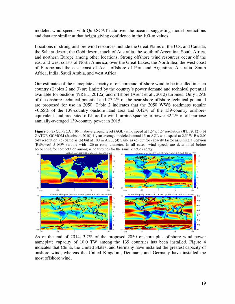
19

modeled wind speeds with QuikSCAT data over the oceans, suggesting model predictions and data are similar at that height giving confidence in the 100-m values. Locations of strong onshore wind resources include the Great Plains of the U.S. and Canada, the Sahara desert, the Gobi desert, much of Australia, the south of Argentina, South Africa, and northern Europe among other locations. Strong offshore wind resources occur off the east and west coasts of North America, over the Great Lakes, the North Sea, the west coast of Europe and the east coast of Asia, offshore of Peru and Argentina, Australia, South Africa, India, Saudi Arabia, and west Africa. Our estimates of the nameplate capacity of onshore and offshore wind to be installed in each country (Tables 2 and 3) are limited by the country’s power demand and technical potential available for onshore (NREL, 2012a) and offshore (Arent et al., 2012) turbines. Only 3.5% of the onshore technical potential and 27.2% of the near-shore offshore technical potential are proposed for use in 2050. Table 2 indicates that the 2050 WWS roadmaps require ~0.65% of the 139-country onshore land area and 0.42% of the 139-country onshore-equivalent land area sited offshore for wind-turbine spacing to power 32.2% of all-purpose annually-averaged 139-country power in 2015. Figure 3. (a) QuikSCAT 10-m above ground level (AGL) wind speed at 1.5o x 1.5o resolution (JPL, 2012), (b) GATOR-GCMOM (Jacobson, 2010) 4-year-average modeled annual 15-m AGL wind speed at 2.5o W-E x 2.0o S-N resolution, (c) Same as (b) but at 100 m AGL, (d) Same as (c) but for capacity factor assuming a Senvion (RePower) 5 MW turbine with 126-m rotor diameter. In all cases, wind speeds are determined before accounting for competition among wind turbines for the same kinetic energy.

As of the end of 2014, 3.7% of the proposed 2050 onshore plus offshore wind power nameplate capacity of 10.0 TW among the 139 countries has been installed. Figure 4 indicates that China, the United States, and Germany have installed the greatest capacity of onshore wind, whereas the United Kingdom, Denmark, and Germany have installed the most offshore wind.

a) Quickscat 2004-2008 wind speed 10 m AGL (m/s)

0

2

4

6

8

10

12

-180 -90 0 90 180-90

0

90 b) Annual wind speed 15 m AGL (m/s) (global: 6.7; land: 4.8; sea: 7.5)

0

2

4

6

8

10

12

-180 -90 0 90 180-90

0

90

c) Annual wind speed (m/s) 100 m AGL (global: 8.9; land: 7.9; sea: 9.3)

0

2

4

6

8

10

12

14

-180 -90 0 90 180-90

0

90d) Annual capacity factor (--) 100 m AGL (global: 0.436; land: 0.34; sea: 0.47)

0

0.1

0.2

0.3

0.4

0.5

0.6

0.7

-180 -90 0 90 180-90

0

90

20

Figure 4. Installed onshore and offshore wind power by country as of the end of 2014. Capacity is determined first from GWEC (2014) year-end values for 2014, followed by IEA (2014b) capacity estimates for 2014, then IEA (2015) capacity estimates for 2011.

21

5.2. Solar Figure 5 shows annually averaged modeled solar irradiance worldwide accounting for sun angles, day/night, and clouds. The best solar resources are broadly between 40 oN and 40 oS. The new land area in 2050 required for non-rooftop solar under the plan here is equivalent to ~0.28% of the 139-country land area (Figure 5). Figure 5. Modeled annually averaged downward direct plus diffuse solar irradiance at the ground (kWh/m2/day) worldwide. The model used is GATOR-GCMOM (Jacobson, 2010), which simulates clouds, aerosols gases, weather, radiation fields, and variations in surface albedo over time. The model is run with horizontal resolution of 2.5o W-E x 2.0o S-N.

Table 4 provides estimates of each country’s maximum rooftop PV nameplate capacity. The proposed capacity for each country, summed in Table 2, is limited by the values in Table 4. Rooftops considered include those on residential, commercial, and governmental buildings, and garages, carports, parking lots, and parking structures associated with these buildings. Commercial and governmental buildings include all non-residential buildings except manufacturing, industrial, and military buildings. Commercial buildings include schools. The total residential rooftop area suitable for PV in each country in 2050 is calculated first by extrapolating the fraction of 2050 population living in urban versus rural areas linearly but with upper limits from 2005-2014 urban fraction data (World Bank, 2015c). Projected 2050 population in each country is then divided between rural and urban population. Population in each case is then multiplied by floor area per capita by country (assumed the same for rural and urban homes) from Entranze Data Tool (2015) for European countries, IEA (2005) for a few additional countries, and IEA (2014a) for remaining regions of the world. The result is finally multiplied by the utilization factor (UF), which is the ratio of the usable rooftop area to ground floor area. For rural areas in each country, UF=0.2. Eiffert et al. (2003) estimate UF=0.4 for rooftops and 0.15 for facades, but for single-family rural residential homes, we assume shading reduces the UF to 0.2. For urban areas, we assume UF=0.4 but divide the urban area population by the number of floors in each urban complex

Annual down solar irradiance at ground (kWh/m2/d) (global: 4.4; land: 4.3; sea: 4.5)

0

1

2

3

4

5

6

7

-180 -90 0 90 180-90

0

90

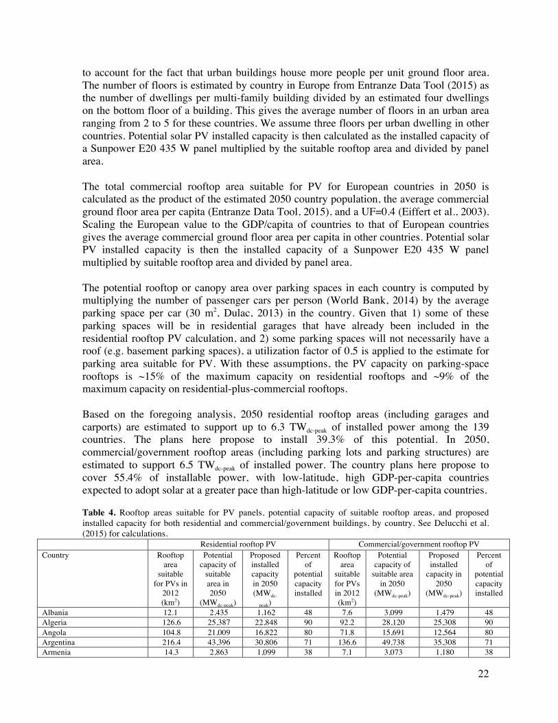
22

to account for the fact that urban buildings house more people per unit ground floor area. The number of floors is estimated by country in Europe from Entranze Data Tool (2015) as the number of dwellings per multi-family building divided by an estimated four dwellings on the bottom floor of a building. This gives the average number of floors in an urban area ranging from 2 to 5 for these countries. We assume three floors per urban dwelling in other countries. Potential solar PV installed capacity is then calculated as the installed capacity of a Sunpower E20 435 W panel multiplied by the suitable rooftop area and divided by panel area. The total commercial rooftop area suitable for PV for European countries in 2050 is calculated as the product of the estimated 2050 country population, the average commercial ground floor area per capita (Entranze Data Tool, 2015), and a UF=0.4 (Eiffert et al., 2003). Scaling the European value to the GDP/capita of countries to that of European countries gives the average commercial ground floor area per capita in other countries. Potential solar PV installed capacity is then the installed capacity of a Sunpower E20 435 W panel multiplied by suitable rooftop area and divided by panel area. The potential rooftop or canopy area over parking spaces in each country is computed by multiplying the number of passenger cars per person (World Bank, 2014) by the average parking space per car (30 m2, Dulac, 2013) in the country. Given that 1) some of these parking spaces will be in residential garages that have already been included in the residential rooftop PV calculation, and 2) some parking spaces will not necessarily have a roof (e.g. basement parking spaces), a utilization factor of 0.5 is applied to the estimate for parking area suitable for PV. With these assumptions, the PV capacity on parking-space rooftops is ~15% of the maximum capacity on residential rooftops and ~9% of the maximum capacity on residential-plus-commercial rooftops. Based on the foregoing analysis, 2050 residential rooftop areas (including garages and carports) are estimated to support up to 6.3 TWdc-peak of installed power among the 139 countries. The plans here propose to install 39.3% of this potential. In 2050, commercial/government rooftop areas (including parking lots and parking structures) are estimated to support 6.5 TWdc-peak of installed power. The country plans here propose to cover 55.4% of installable power, with low-latitude, high GDP-per-capita countries expected to adopt solar at a greater pace than high-latitude or low GDP-per-capita countries. Table 4. Rooftop areas suitable for PV panels, potential capacity of suitable rooftop areas, and proposed installed capacity for both residential and commercial/government buildings, by country. See Delucchi et al. (2015) for calculations.

Residential rooftop PV Commercial/government rooftop PV Country Rooftop

area suitable

for PVs in 2012 (km2)

Potential capacity of

suitable area in 2050

(MWdc-peak)

Proposed installed capacity in 2050 (MWdc-

peak)

Percent of

potential capacity installed

Rooftop area

suitable for PVs in 2012 (km2)

Potential capacity of

suitable area in 2050

(MWdc-peak)

Proposed installed

capacity in 2050

(MWdc-peak)

Percent of

potential capacity installed

Albania 12.1 2,435 1,162 48 7.6 3,099 1,479 48 Algeria 126.6 25,387 22,848 90 92.2 28,120 25,308 90 Angola 104.8 21,009 16,822 80 71.8 15,691 12,564 80 Argentina 216.4 43,396 30,806 71 136.6 49,738 35,308 71 Armenia 14.3 2,863 1,099 38 7.1 3,073 1,180 38

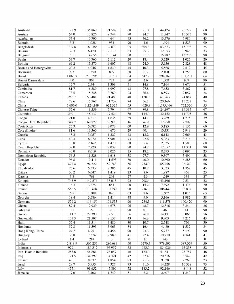
23

Australia 178.9 35,869 21,582 60 91.0 44,424 26,729 60 Austria 54.0 10,826 9,744 90 24.7 11,747 10,573 90 Azerbaijan 53.4 10,700 4,644 43 36.2 13,776 5,980 43 Bahrain 5.2 1,038 934 90 4.6 1,694 1,525 90 Bangladesh 799.8 160,388 39,670 25 305.3 63,873 15,798 25 Belarus 32.3 6,470 2,119 33 25.3 12,053 3,948 33 Belgium 73.1 14,655 13,144 90 31.7 15,282 13,706 90 Benin 53.7 10,760 2,112 20 18.4 5,229 1,026 20 Bolivia 69.2 13,870 6,607 48 24.0 5,936 2,828 48 Bosnia and Herzegovina 20.2 4,046 1,830 45 10.3 5,568 2,519 45 Botswana 6.7 1,350 809 60 6.3 2,100 1,258 60 Brazil 1,063.7 213,295 135,738 64 647.2 294,162 187,201 64 Brunei Darussalam 4.0 803 723 90 2.6 1,008 907 90 Bulgaria 12.7 2,544 1,303 51 14.8 7,164 3,670 51 Cambodia 81.7 16,389 6,997 43 27.8 7,652 3,267 43 Cameroon 78.5 15,748 3,769 24 36.4 8,593 2,057 24 Canada 266.7 53,481 21,480 40 128.0 61,963 24,887 40 Chile 78.6 15,767 11,739 74 56.1 20,466 15,237 74 China 5,606.0 1,124,149 622,325 55 4029.9 1,395,466 772,526 55 Chinese Taipei 57.6 11,559 7,794 67 89.8 24,197 16,315 67 Colombia 240.1 48,137 17,524 36 114.0 32,152 11,705 36 Congo 21.0 4,217 1,635 39 14.1 3,289 1,275 39 Congo, Dem. Republic 347.7 69,727 10,920 16 76.9 17,858 2,797 16 Costa Rica 25.3 5,082 3,073 60 12.9 5,185 3,135 60 Cote d'Ivoire 81.6 16,360 4,670 29 40.4 10,331 2,949 29 Croatia 15.2 3,057 1,327 43 13.2 6,143 2,666 43 Cuba 40.3 8,072 5,901 73 22.6 5,083 3,716 73 Cyprus 10.8 2,162 1,470 68 5.4 2,335 1,588 68 Czech Republic 39.0 7,820 7,038 90 24.2 12,557 11,301 90 Denmark 40.0 8,019 2,026 25 18.2 8,293 2,095 25 Dominican Republic 56.5 11,328 6,618 58 27.7 9,397 5,490 58 Ecuador 96.8 19,411 11,593 60 40.0 10,690 6,385 60 Egypt 472.4 94,722 52,748 56 254.0 65,258 36,340 56 El Salvador 26.6 5,333 2,385 45 10.2 3,023 1,352 45 Eritrea 30.2 6,047 1,419 23 8.6 1,987 466 23 Estonia 3.8 761 204 27 2.3 1,249 334 27 Ethiopia 745.9 149,576 33,013 22 208.4 43,196 9,534 22 Finland 16.3 3,275 654 20 15.2 7,392 1,476 20 France 566.5 113,604 102,243 90 216.9 106,447 95,802 90 Gabon 6.5 1,308 826 63 7.6 1,607 1,015 63 Georgia 18.4 3,686 1,414 38 9.0 5,166 1,982 38 Germany 579.2 116,150 104,535 90 234.5 111,578 100,420 90 Ghana 89.4 17,929 4,678 26 48.7 12,816 3,344 26 Gibraltar 0.1 22 20 90 0.1 46 41 90 Greece 111.7 22,390 12,513 56 26.8 14,431 8,065 56 Guatemala 107.3 21,507 9,157 43 36.3 9,903 4,216 43 Haiti 57.4 11,514 3,480 30 10.7 2,548 770 30 Honduras 57.8 11,593 3,963 34 16.4 4,480 1,532 34 Hong Kong, China 24.7 4,951 4,456 90 23.3 5,777 5,199 90 Hungary 36.8 7,374 2,989 41 22.4 10,710 4,341 41 Iceland 1.4 284 0 0 1.1 543 0 0 India 2,818.9 565,256 280,689 50 3270.3 779,505 387,079 50 Indonesia 929.1 186,312 95,952 52 663.0 184,926 95,238 52 Iran, Islamic Republic 283.6 56,861 26,057 46 164.0 51,841 23,757 46 Iraq 171.5 34,397 14,321 42 87.4 20,516 8,542 42 Ireland 40.1 8,032 1,854 23 21.3 9,828 2,268 23 Israel 29.7 5,955 4,327 73 31.6 14,228 10,338 73 Italy 457.1 91,652 47,890 52 183.2 92,146 48,148 52 Jamaica 17.0 3,402 1,749 51 6.2 2,607 1,340 51

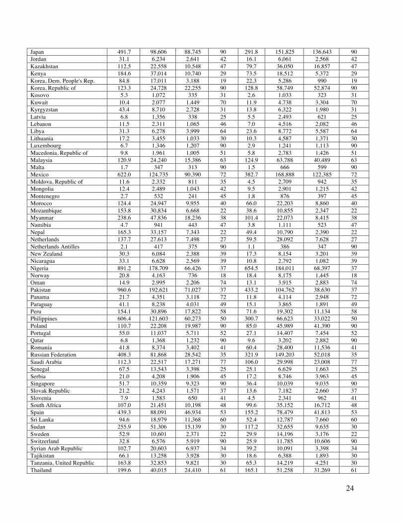
24

Japan 491.7 98,606 88,745 90 291.8 151,825 136,643 90 Jordan 31.1 6,234 2,641 42 16.1 6,061 2,568 42 Kazakhstan 112.5 22,558 10,548 47 79.7 36,050 16,857 47 Kenya 184.6 37,014 10,740 29 73.5 18,512 5,372 29 Korea, Dem. People's Rep. 84.8 17,011 3,188 19 22.3 5,286 990 19 Korea, Republic of 123.3 24,728 22,255 90 128.8 58,749 52,874 90 Kosovo 5.3 1,072 335 31 2.6 1,033 323 31 Kuwait 10.4 2,077 1,449 70 11.9 4,738 3,304 70 Kyrgyzstan 43.4 8,710 2,728 31 13.8 6,322 1,980 31 Latvia 6.8 1,356 338 25 5.5 2,493 621 25 Lebanon 11.5 2,311 1,065 46 7.0 4,516 2,082 46 Libya 31.3 6,278 3,999 64 23.6 8,772 5,587 64 Lithuania 17.2 3,455 1,033 30 10.3 4,587 1,371 30 Luxembourg 6.7 1,346 1,207 90 2.9 1,241 1,113 90 Macedonia, Republic of 9.8 1,961 1,005 51 5.8 2,783 1,426 51 Malaysia 120.9 24,240 15,386 63 124.9 63,788 40,489 63 Malta 1.7 347 313 90 1.5 666 599 90 Mexico 622.0 124,735 90,390 72 382.7 168,888 122,385 72 Moldova, Republic of 11.6 2,332 811 35 4.5 2,709 942 35 Mongolia 12.4 2,489 1,043 42 9.5 2,901 1,215 42 Montenegro 2.7 532 241 45 1.8 876 397 45 Morocco 124.4 24,947 9,955 40 66.0 22,203 8,860 40 Mozambique 153.8 30,834 6,668 22 38.6 10,855 2,347 22 Myanmar 238.6 47,836 18,236 38 101.4 22,073 8,415 38 Namibia 4.7 941 443 47 3.8 1,111 523 47 Nepal 165.3 33,157 7,343 22 49.4 10,790 2,390 22 Netherlands 137.7 27,613 7,498 27 59.5 28,092 7,628 27 Netherlands Antilles 2.1 417 375 90 1.1 386 347 90 New Zealand 30.3 6,084 2,388 39 17.3 8,154 3,201 39 Nicaragua 33.1 6,628 2,569 39 10.8 2,792 1,082 39 Nigeria 891.2 178,709 66,426 37 654.5 184,011 68,397 37 Norway 20.8 4,163 736 18 18.4 8,175 1,445 18 Oman 14.9 2,995 2,206 74 13.1 3,915 2,883 74 Pakistan 960.6 192,621 71,027 37 433.2 104,762 38,630 37 Panama 21.7 4,351 3,118 72 11.8 4,114 2,948 72 Paraguay 41.1 8,238 4,031 49 15.1 3,865 1,891 49 Peru 154.1 30,896 17,822 58 71.6 19,302 11,134 58 Philippines 606.4 121,603 60,273 50 300.7 66,623 33,022 50 Poland 110.7 22,208 19,987 90 85.0 45,989 41,390 90 Portugal 55.0 11,037 5,711 52 27.1 14,407 7,454 52 Qatar 6.8 1,368 1,232 90 9.6 3,202 2,882 90 Romania 41.8 8,374 3,402 41 60.4 28,400 11,536 41 Russian Federation 408.3 81,868 28,542 35 321.9 149,203 52,018 35 Saudi Arabia 112.3 22,517 17,271 77 106.0 29,998 23,008 77 Senegal 67.5 13,543 3,398 25 25.1 6,629 1,663 25 Serbia 21.0 4,208 1,906 45 17.2 8,746 3,963 45 Singapore 51.7 10,359 9,323 90 36.4 10,039 9,035 90 Slovak Republic 21.2 4,243 1,571 37 13.6 7,182 2,660 37 Slovenia 7.9 1,583 650 41 4.5 2,341 962 41 South Africa 107.0 21,451 10,198 48 99.6 35,152 16,712 48 Spain 439.3 88,091 46,934 53 155.2 78,479 41,813 53 Sri Lanka 94.6 18,979 11,368 60 52.4 12,787 7,660 60 Sudan 255.9 51,306 15,139 30 117.2 32,655 9,635 30 Sweden 52.9 10,601 2,371 22 29.9 14,196 3,176 22 Switzerland 32.8 6,576 5,919 90 25.9 11,785 10,606 90 Syrian Arab Republic 102.7 20,603 6,937 34 39.2 10,091 3,398 34 Tajikistan 66.1 13,258 3,928 30 18.6 6,388 1,893 30 Tanzania, United Republic 163.8 32,853 9,821 30 65.3 14,219 4,251 30 Thailand 199.6 40,015 24,410 61 165.1 51,258 31,269 61

25

Togo 40.4 8,097 1,386 17 12.2 2,558 438 17 Trinidad and Tobago 6.1 1,220 1,098 90 2.9 1,181 1,063 90 Tunisia 36.9 7,401 3,591 49 23.4 8,105 3,933 49 Turkey 429.1 86,050 45,069 52 243.7 80,238 42,025 52 Turkmenistan 21.1 4,240 2,347 55 20.4 8,278 4,583 55 Ukraine 150.3 30,140 11,089 37 83.8 42,433 15,611 37 United Arab Emirates 21.6 4,340 3,906 90 23.1 7,199 6,479 90 United Kingdom 199.4 39,990 10,859 27 222.0 108,727 29,523 27 United States of America 3,723.1 746,577 494,885 66 1507.1 683,515 453,083 66 Uruguay 14.0 2,803 1,690 60 8.5 3,903 2,353 60 Uzbekistan 124.5 24,969 10,749 43 73.4 14,720 6,337 43 Venezuela 168.7 33,834 19,985 59 91.3 29,302 17,308 59 Vietnam 362.4 72,664 34,414 47 177.0 42,517 20,136 47 Yemen 150.0 30,073 8,078 27 38.8 9,136 2,454 27 Zambia 93.7 18,789 6,353 34 45.4 11,199 3,787 34 Zimbabwe 69.0 13,846 3,735 27 20.5 13,132 3,542 27 World total or average 31,356 6,287,586 3,304,963 39.30 19,070 6,482,448 3,589,760 55.38

Utility-scale PV potential is determined with the NREL Global Solar Opportunity Tool (NREL, 2012b), which gives the utility PV potential (in GW of rated capacity) by country for different resource thresholds. We define the utility-scale PV potential as the potential calculated from the tool in locations exceeding 4 kWh/m2/day. As of the end of 2014, 0.55% of the proposed 2050 PV (residential rooftop, commercial/government rooftop, and utility scale) capacity and 0.37% of the CSP capacity among the 139 countries from Table 2 has been installed. Figure 6 indicates that Germany, China, Japan, and Italy have installed the most PV. Spain, the United States, and India have installed the most CSP. Figure 6. (a) Installed residential, commercial/government, plus utility PV by country and (b) installed CSP by country as of the end of 2014. Total PV is determined first from IEA-PVPS (2015) and IEA (2014b); the ratios of residential : commercial/government : utility PV for 20 European countries and global averages were obtained from EPIA (2014). CSP by country includes operational plants and plants under construction that broke ground before 2015 (CSP World, 2015; NREL, 2015).

26

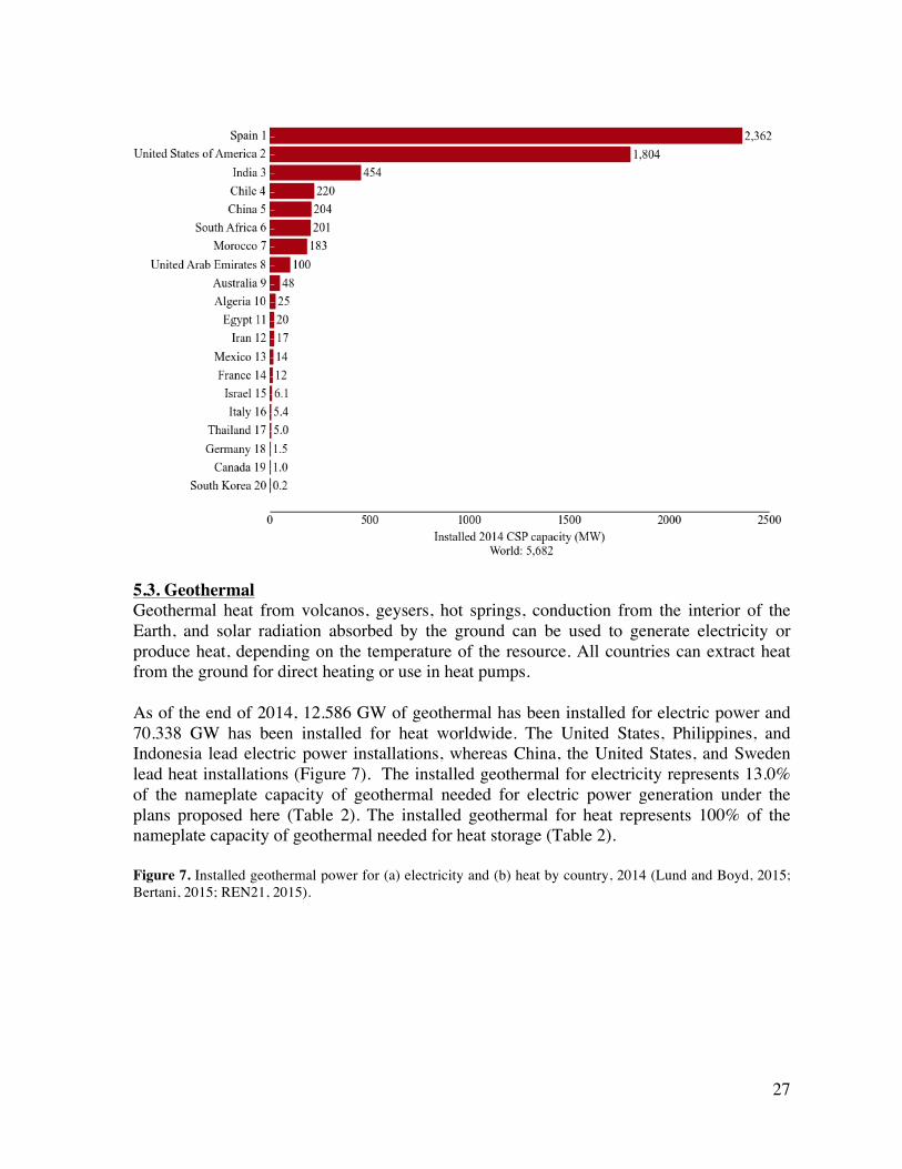
27

5.3. Geothermal Geothermal heat from volcanos, geysers, hot springs, conduction from the interior of the Earth, and solar radiation absorbed by the ground can be used to generate electricity or produce heat, depending on the temperature of the resource. All countries can extract heat from the ground for direct heating or use in heat pumps. As of the end of 2014, 12.586 GW of geothermal has been installed for electric power and 70.338 GW has been installed for heat worldwide. The United States, Philippines, and Indonesia lead electric power installations, whereas China, the United States, and Sweden lead heat installations (Figure 7). The installed geothermal for electricity represents 13.0% of the nameplate capacity of geothermal needed for electric power generation under the plans proposed here (Table 2). The installed geothermal for heat represents 100% of the nameplate capacity of geothermal needed for heat storage (Table 2). Figure 7. Installed geothermal power for (a) electricity and (b) heat by country, 2014 (Lund and Boyd, 2015; Bertani, 2015; REN21, 2015).

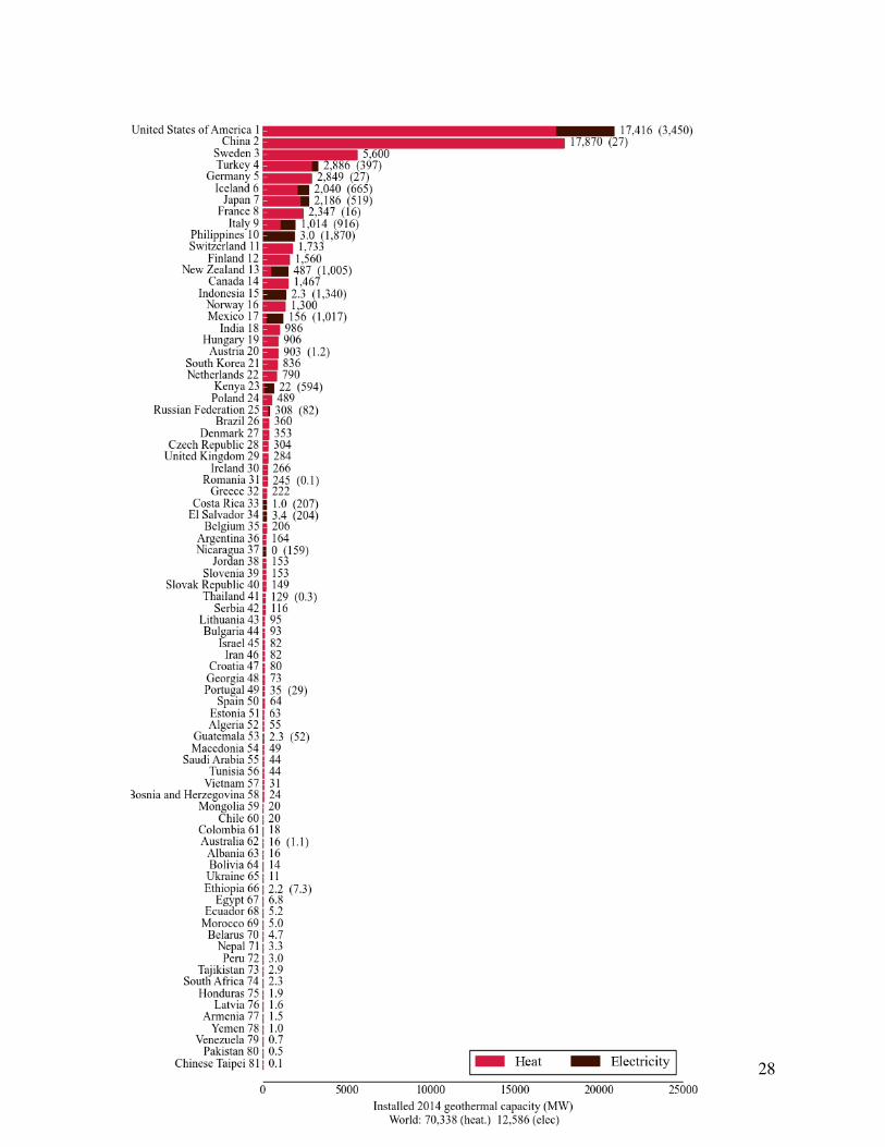
28

29

The average capacity factor of installed geothermal for electricity worldwide based on 2012 data is ~70.3% (IEA, 2015). However, this is not a technical or economic limit, and in a 100% WWS system the capacity factor for geothermal could be higher than this. Therefore, the roadmaps here assume that the capacity factor of geothermal will increase to 90.5% by 2050. They call for a 139-country-total of 96.6 GW of installed geothermal for electricity producing 87.0 GW of delivered power in 2050. 5.4. Hydropower In 2012, conventional (small and large) hydropower provided ~16.5% of the world electric power supply (IEA, 2014a). 2014 installations of hydropower were ~1.143 TW (Figure 8). Given the world-averaged capacity factor for hydropower of ~41.8% in 2012 (IEA, 2014a), this implies hydropower delivered electricity in 2014 of ~477.8 GW (4185 TWh/yr). Figure 8 shows the distribution of installed conventional hydropower by country. China, the United States, Brazil, and Canada lead in installations. However, the countries of the world with the greatest percentage of their electric power production from hydropower in 2012 include, in order: Albania (100%), Paraguay (100%), Montenegro (99.9%), Zambia (99.7%), Tajikistan (99.6%), Democratic Republic of the Congo (99.6%), Nepal (99.5%), Ethiopia (98.7%), Namibia (97.8%), Norway (96.7%), and the Kyrgyz Republic (93.5%). (World Bank, 2015). Thus, 7 countries already produce 99-100% of all their electricity from WWS hydropower. In fact, 22 countries produce more than 70% of all their electricity from hydropower and 36 produce more than 50%, of which 28 are developing countries. Figure 8. Installed conventional hydropower by country in 2014 (IEA, 2014b; IHA, 2015).

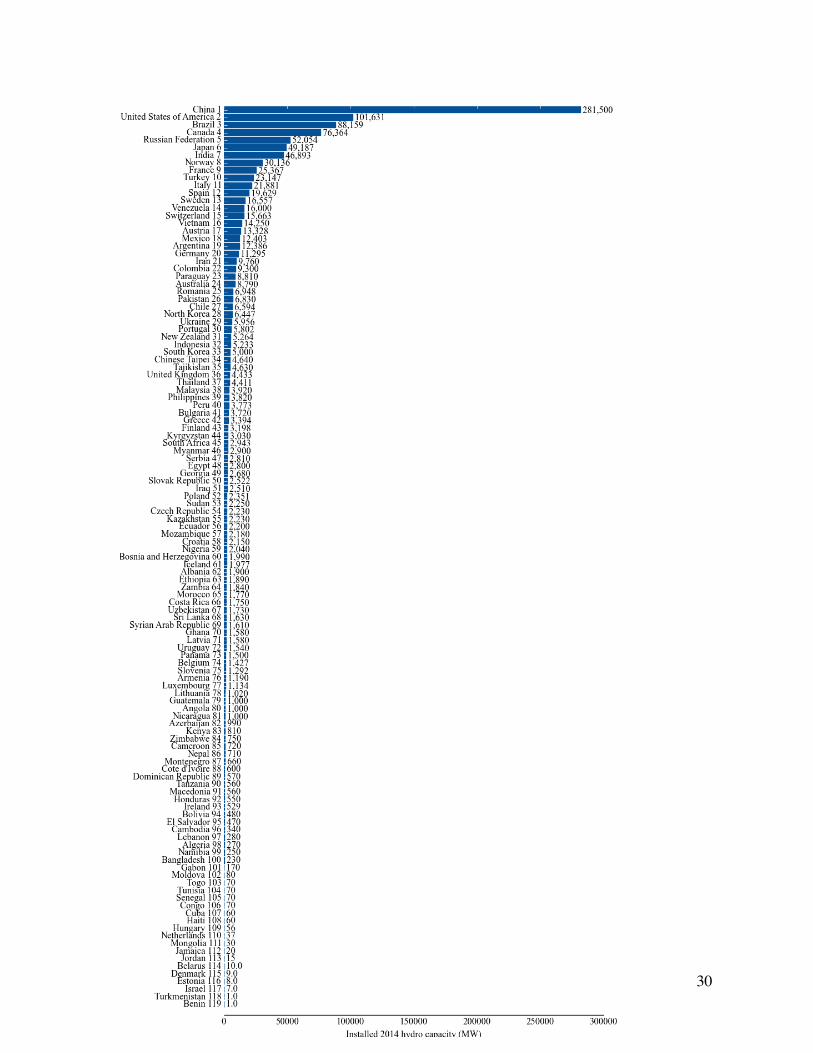
30

31

Under the roadmaps proposed here, conventional hydropower will supply ~4.8% (570.4 GW) of the 139-country 2050 end-use power demand for all purposes (Table 2). However, no new hydropower dams are proposed for installation. Instead, the capacity factor of hydropower will be increased from a 139-country average of ~41.8% to 50% by 2050. Increasing the capacity factor is feasible because existing dams currently produce less than their maximum capacity, mainly because many other dispatchable sources of electricity exist in the current energy system, greatly reducing the need for hydropower to balance supply and demand. However, in some cases, hydropower is not used to its full extent because of other priorities affecting water use, and in a 100% WWS system, these other priorities will remain. Whereas, increasing hydropower capacity factors should be possible, if it is not, additional hydropower capacity can be obtained by powering presently non-powered dams. The U.S., for example, has over 80,000 dams that are not powered at present. Although only a small fraction of these dams can feasibly be powered, DOE (2012) estimates that the potential amounts to ~12 GW of capacity in the contiguous 48 states. 5.5. Tidal and Wave Worldwide by the end of 2014, a total of ~534 MW of ocean devices (mostly tidal barrages) had been installed. Figure 9 indicates these are mostly from two large plants in South Korea and France and smaller plants in Canada and the United Kingdom. Figure 9. Installed ocean power by country in 2014 (IEA 2014b). Ocean power includes tidal rise and fall, ocean and tidal currents, wave power, ocean thermal energy conversion, and salinity gradients. Nearly all existing capacity in the figure arises from tidal barrages.

32

Under the roadmaps here, tidal is proposed to contribute ~0.068%, or ~8.03 GW, of the 139-country end-use delivered power in 2050 (Table 2). This requires a nameplate capacity of ~32.6 GW installed of which ~1.6% has been installed as of the end of 2014. The needed nameplate capacity is much less than the estimated world technical potential of ~556 GW installed (1200 TWh/yr or 137 GW delivered power) (Marine Renewables Canada, 2015). Some countries with significant tidal potential include Australia (3.8 GW nameplate capacity), Canada (171 GW), France (16 GW), Ireland (107 GW), Japan (3 GW), United Kingdom (8 GW), and the United States (116 GW) (Marine Renewables Canada, 2015). Wave power is proposed here to contribute ~0.72%, or ~85.3 GW, of the 139-country end-use power demand in 2050 (Table 2). This requires a nameplate installation of ~372 GW, which is much less than the world technical potential for the 139 countries considered of ~4.362 GW installed (8,850 TWh/yr, or 1010 GW delivered) (Marine Renewables Canada, 2015 but assuming 70% exclusion zones). Some of countries with significant wave potential include Australia (192 GW installed), Canada (275 GW), France (14 GW), Japan (13 GW), Ireland (3 GW), Norway (59 GW), United Kingdom (6 GW), and the United States (263 GW) (Marine Renewables Canada, 2015). 6. Matching Electric Power Supply with Demand An important requirement for 100% WWS roadmaps is that the grid remains reliable. To that end, Jacobson et al. (2015b) developed and applied a grid integration model to determine the quantities and costs of storage devices needed to ensure that a 100% WWS system developed for each of the 48 contiguous U.S. states, when integrated across all such states, could match load without loss every 30 s for 6 years (2050-2055) while accounting for the variability and uncertainty of WWS resources. Wind and solar time-series were derived from 3-D global model simulations that accounted for extreme events and competition among wind turbines for kinetic energy and the feedback of extracted solar radiation to roof and surface temperatures. Solutions were obtained by prioritizing storage for excess heat (in soil and water) and electricity (in ice, water, phase-change material tied to CSP, pumped hydro, and hydrogen), using hydropower only as a last resort, and using demand response to shave periods of excess demand over supply. No stationary storage batteries, biomass, nuclear power, or natural gas were needed. Frequency regulation of the grid was provided by ramping up/down hydropower, stored CSP or pumped hydro; ramping down other WWS generators and storing the electricity in heat, cold, or hydrogen instead of curtailment; and using demand response. Multiple low-cost stable solutions to the grid integration problem across the 48 contiguous U.S. states were obtained, suggesting that maintaining grid reliability upon 100% conversion to WWS in that region is a solvable problem. The mean U.S.-averaged levelized cost of energy in that study, accounting for storage transmission, distribution, maintenance, and array losses, was ~10.6 ¢/kWh for electricity and ~11.4 ¢/kWh for all energy in 2013 dollars.

33

For the 139-country roadmaps here, similar grid integration studies are being performed (Jacobson et al., 2016b). For these studies, the 139 countries are divided into 20 groups of countries or individual island countries where both time-dependent demand for and supply of WWS energy are aggregated for use in the same grid integration model as was used in the 50-state study. Additional CSP and solar thermal collectors for peaking/storage are also being added to each country’s energy supply to help firm the grid, as in that study. Geothermal heat in 2014 by country is assumed also to exist in 2050, enhancing the ability of the entire heat and power system to remain stable. For each region, electricity storage and heat/cold storage are being used. Stable solutions have been obtained to date for all 20 regions and countries suggesting grid reliability is not a barrier to 100% clean, renewable WWS energy systems in the 139 countries considered. 7. Costs of Electric Power Generation In this section, current and future full social costs (including capital, land, operating, maintenance, storage, fuel, transmission, and externality costs) of WWS electric power generators versus non-WWS conventional fuel generators are estimated. These costs do not include the costs of storage necessary to keep the grid stable, which are being quantified in Jacobson et al. (2016b), except for the cost of storage associated with CSP, which is included here. The estimates here are based on current cost data and trend projections for individual generator types. The estimates are only a rough approximation of costs in a future optimized renewable energy system. Table 5 presents 2013 and 2050 139-country weighted average estimates of fully annualized levelized business costs of electric power generation for conventional fuels and WWS technologies. The table indicates that the 2013 business costs of hydropower, onshore wind, utility-scale solar PV, and solar thermal for heat are already similar to or less than the costs of natural gas combined cycle. Residential and commercial PV, offshore wind, tidal, and wave are more expensive. However, residential rooftop PV costs are given as if PV is purchased for an individual household. A common business model today is where multiple households contract together with a solar provider to decrease the average cost. By 2050, the costs of all WWS technologies are expected to drop, most significantly for offshore wind, tidal, wave, rooftop PV, CSP, and utility PV, whereas conventional fuel costs are expected to rise. Because WWS technologies have zero fuel costs, the drop in their costs over time is due primarily to technology improvements. WWS costs are expected to decline also due to less expensive manufacturing and streamlined project deployment from increased economies of scale. Conventional fuels, on the other hand, face rising costs over time due to higher labor and transport costs for mining, transporting, and processing fuels continuously over the lifetime of fossil-fuel plants. Table 5. Approximate fully annualized, unsubsidized 2013 and 2050 U.S.-averaged costs of delivered electricity, including generation, short- and long-distance transmission, distribution, and storage, but not including external costs, for conventional fuels and WWS power (2013 U.S. $/kWh-delivered). Technology Technology year 2013 Technology year 2050

LCHB HCLB Average LCHB HCLB Average Advanced pulverized coal 0.083 0.113 0.098 0.079 0.107 0.093 Advanced pulverized coal w/CC 0.116 0.179 0.148 0.101 0.151 0.126 IGCC coal 0.094 0.132 0.113 0.084 0.115 0.100

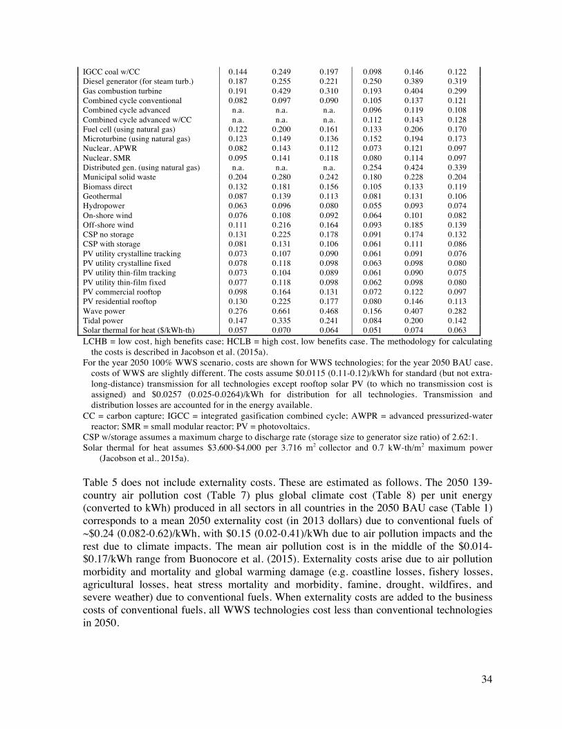
34

IGCC coal w/CC 0.144 0.249 0.197 0.098 0.146 0.122 Diesel generator (for steam turb.) 0.187 0.255 0.221 0.250 0.389 0.319 Gas combustion turbine 0.191 0.429 0.310 0.193 0.404 0.299 Combined cycle conventional 0.082 0.097 0.090 0.105 0.137 0.121 Combined cycle advanced n.a. n.a. n.a. 0.096 0.119 0.108 Combined cycle advanced w/CC n.a. n.a. n.a. 0.112 0.143 0.128 Fuel cell (using natural gas) 0.122 0.200 0.161 0.133 0.206 0.170 Microturbine (using natural gas) 0.123 0.149 0.136 0.152 0.194 0.173 Nuclear, APWR 0.082 0.143 0.112 0.073 0.121 0.097 Nuclear, SMR 0.095 0.141 0.118 0.080 0.114 0.097 Distributed gen. (using natural gas) n.a. n.a. n.a. 0.254 0.424 0.339 Municipal solid waste 0.204 0.280 0.242 0.180 0.228 0.204 Biomass direct 0.132 0.181 0.156 0.105 0.133 0.119 Geothermal 0.087 0.139 0.113 0.081 0.131 0.106 Hydropower 0.063 0.096 0.080 0.055 0.093 0.074 On-shore wind 0.076 0.108 0.092 0.064 0.101 0.082 Off-shore wind 0.111 0.216 0.164 0.093 0.185 0.139 CSP no storage 0.131 0.225 0.178 0.091 0.174 0.132 CSP with storage 0.081 0.131 0.106 0.061 0.111 0.086 PV utility crystalline tracking 0.073 0.107 0.090 0.061 0.091 0.076 PV utility crystalline fixed 0.078 0.118 0.098 0.063 0.098 0.080 PV utility thin-film tracking 0.073 0.104 0.089 0.061 0.090 0.075 PV utility thin-film fixed 0.077 0.118 0.098 0.062 0.098 0.080 PV commercial rooftop 0.098 0.164 0.131 0.072 0.122 0.097 PV residential rooftop 0.130 0.225 0.177 0.080 0.146 0.113 Wave power 0.276 0.661 0.468 0.156 0.407 0.282 Tidal power 0.147 0.335 0.241 0.084 0.200 0.142 Solar thermal for heat ($/kWh-th) 0.057 0.070 0.064 0.051 0.074 0.063 LCHB = low cost, high benefits case; HCLB = high cost, low benefits case. The methodology for calculating

the costs is described in Jacobson et al. (2015a). For the year 2050 100% WWS scenario, costs are shown for WWS technologies; for the year 2050 BAU case,

costs of WWS are slightly different. The costs assume $0.0115 (0.11-0.12)/kWh for standard (but not extra-long-distance) transmission for all technologies except rooftop solar PV (to which no transmission cost is assigned) and $0.0257 (0.025-0.0264)/kWh for distribution for all technologies. Transmission and distribution losses are accounted for in the energy available.

CC = carbon capture; IGCC = integrated gasification combined cycle; AWPR = advanced pressurized-water reactor; SMR = small modular reactor; PV = photovoltaics.

CSP w/storage assumes a maximum charge to discharge rate (storage size to generator size ratio) of 2.62:1. Solar thermal for heat assumes $3,600-$4,000 per 3.716 m2 collector and 0.7 kW-th/m2 maximum power

(Jacobson et al., 2015a). Table 5 does not include externality costs. These are estimated as follows. The 2050 139-country air pollution cost (Table 7) plus global climate cost (Table 8) per unit energy (converted to kWh) produced in all sectors in all countries in the 2050 BAU case (Table 1) corresponds to a mean 2050 externality cost (in 2013 dollars) due to conventional fuels of ~$0.24 (0.082-0.62)/kWh, with $0.15 (0.02-0.41)/kWh due to air pollution impacts and the rest due to climate impacts. The mean air pollution cost is in the middle of the $0.014-$0.17/kWh range from Buonocore et al. (2015). Externality costs arise due to air pollution morbidity and mortality and global warming damage (e.g. coastline losses, fishery losses, agricultural losses, heat stress mortality and morbidity, famine, drought, wildfires, and severe weather) due to conventional fuels. When externality costs are added to the business costs of conventional fuels, all WWS technologies cost less than conventional technologies in 2050.

35

Table 6 provides the mean value of the 2013 and 2050 LCOEs weighted among all conventional generators (BAU cases) and WWS generators (WWS case) by country. The table also gives the 2050 energy, health, and global climate cost savings per person. The electric power cost of WWS in 2050 is not directly comparable with the BAU electric power cost, because the latter does not integrate transportation, heating/cooling, or industry energy costs. Conventional vehicle fuel costs, for example, are a factor of 4-5 higher than those of electric vehicles, yet the cost of BAU electricity cost in 2050 does not include the transportation cost, whereas the WWS electricity cost does. Nevertheless, based on the comparison, WWS energy in 2050 will save the average 139-country consumer $170/yr in energy costs ($2013 dollars). In addition, WWS will save $2,880/yr in health costs, and $1,930/yr in global climate costs. The total up-front capital cost of the 2050 WWS system (for both average annual power and peaking storage in Table 2) for the 139 countries is ~$100 trillion for the 49.2 TW of installed capacity needed (~$2.03 million/MW). Table 6. Mean values of the levelized cost of energy (LCOE) for conventional fuels (BAU) in 2013 and 2050 and for WWS fuels in 2050. The LCOE estimates do not include externality costs. The 2013 and 2050 values are used to calculate energy cost savings per person per year in each country (see footnotes). Health and climate cost savings per person per year are derived from data in Section 8. All costs are in 2013 dollars.

Country (a) 2013

LCOE of BAU

(¢/kWh)

(b) 2050

LCOE of BAU

(¢/kWh)

(c) 2050

LCOE of WWS

(¢/kWh)

(d) 2050

Average electricity

cost savings per person per

year ($/per-son/yr)

(e) 2050

Average air quality

health cost savings per person per year due to

WWS ($/person/yr)

(f) 2050

Average climate cost savings to world per person per year due to

WWS ($/person/yr)

(g) 2050

Average energy + health +

world climate cost savings due to WWS ($/person/yr)

Albania 7.98 6.90 6.92 82 1,823 818 2,723 Algeria 8.95 12.01 7.28 157 1,203 1,618 2,977 Angola 8.26 8.40 13.63 -9 2,289 340 2,619 Argentina 9.07 10.68 10.60 83 1,376 1,837 3,296 Armenia 9.60 9.50 5.89 175 3,560 676 4,411 Australia 10.83 10.37 8.49 418 776 5,871 7,064 Austria 9.55 9.17 6.45 456 4,311 4,162 8,929 Azerbaijan 8.83 11.38 7.72 226 3,877 2,341 6,444 Bahrain 8.96 12.06 7.29 1,419 2,363 6,739 10,522 Bangladesh 8.99 11.93 6.90 28 2,220 130 2,378 Belarus 8.97 12.04 6.35 699 10,935 4,030 15,664 Belgium 11.31 10.70 6.88 581 4,570 5,003 10,155 Benin 9.02 12.08 6.19 10 2,475 123 2,608 Bolivia 8.94 10.48 8.69 22 542 573 1,138 Bosnia and Herzegovina 10.34 9.07 6.37 229 2,323 4,096 6,648 Botswana 11.33 9.94 7.25 131 1,186 896 2,213 Brazil 8.87 7.97 8.07 70 515 923 1,508 Brunei Darussalam 8.98 12.07 6.83 1,310 258 8,257 9,825 Bulgaria 11.30 9.85 5.78 950 6,253 4,457 11,660 Cambodia 9.19 11.84 9.92 15 802 110 926 Cameroon 8.32 8.29 5.85 19 2,492 108 2,619 Canada 9.35 8.48 9.89 164 2,616 6,109 8,888 Chile 10.03 10.01 9.12 288 1,588 2,302 4,178 China 10.91 9.62 7.40 342 5,329 3,823 9,494 Chinese Taipei 10.91 9.62 10.19 376 5,647 6,553 12,576

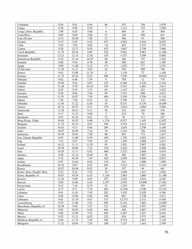
36

Colombia 8.56 8.01 6.49 40 253 784 1,078 Congo 8.36 8.90 9.19 7 1,132 122 1,260 Congo, Dem. Republic 7.99 6.93 5.00 4 489 10 504 Costa Rica 9.89 8.89 9.68 23 148 650 821 Cote d'Ivoire 8.75 10.58 7.28 21 396 83 500 Croatia 9.33 9.45 6.54 437 4,934 2,654 8,025 Cuba 5.43 7.05 9.60 -18 625 2,147 2,755 Cyprus 9.28 12.17 8.54 452 3,867 2,749 7,068 Czech Republic 11.75 10.10 6.00 524 5,041 5,901 11,466 Denmark 13.21 12.15 12.92 145 4,757 3,599 8,500 Dominican Republic 9.24 11.14 10.39 40 366 797 1,203 Ecuador 8.66 9.30 8.78 28 290 862 1,180 Egypt 9.00 11.68 8.15 171 1,835 777 2,783 El Salvador 11.36 11.21 9.82 42 195 509 746 Eritrea 9.02 12.08 11.76 2 1,110 27 1,140 Estonia 11.75 10.36 8.52 586 7,530 10,902 19,018 Ethiopia 8.02 6.96 7.39 0 758 12 770 Finland 10.69 9.62 9.83 335 6,360 5,226 11,921 France 11.48 9.70 10.18 159 3,191 2,462 5,813 Gabon 8.55 9.70 7.23 65 1,147 421 1,632 Georgia 8.20 8.06 7.64 90 3,523 808 4,421 Germany 11.91 10.87 7.50 656 5,189 5,296 11,141 Ghana 7.56 7.59 6.51 14 2,790 121 2,924 Gibraltar 11.44 11.22 6.20 18 8,331 8,139 16,489 Greece 10.74 10.79 8.21 379 3,634 3,684 7,696 Guatemala 11.28 10.51 9.11 18 216 245 478 Haiti 9.17 11.33 9.98 2 215 79 296 Honduras 8.97 10.10 8.61 23 92 312 427 Hong Kong, China 10.65 10.55 6.98 1,176 8,517 3,165 12,857 Hungary 11.19 10.74 4.91 396 5,518 2,431 8,345 Iceland 10.63 9.13 9.84 286 1,016 2,798 4,100 India 10.97 10.05 7.44 70 3,234 726 4,030 Indonesia 10.39 10.91 7.50 80 603 773 1,457 Iran, Islamic Republic 8.93 11.80 6.59 249 1,750 3,052 5,051 Iraq 7.33 9.57 7.65 26 1,299 1,088 2,413 Ireland 10.12 11.11 11.55 93 1,591 2,897 4,581 Israel 10.38 10.80 7.25 354 2,434 3,300 6,088 Italy 10.20 11.17 6.92 486 3,522 2,868 6,876 Jamaica 9.49 12.14 10.65 50 206 1,007 1,263 Japan 9.72 10.36 7.49 429 2,598 5,806 8,833 Jordan 8.97 12.04 8.02 139 761 1,000 1,899 Kazakhstan 10.79 9.87 8.52 284 3,912 6,913 11,109 Kenya 10.57 10.49 8.42 10 357 94 461 Korea, Dem. People's Rep. 9.22 8.14 7.83 19 1,048 1,417 2,484 Korea, Republic of 10.87 10.39 6.35 1,136 2,965 7,089 11,190 Kosovo 11.26 9.89 8.02 297 1,036 2,833 4,165 Kuwait 8.96 12.06 6.44 2,197 2,078 13,008 17,283 Kyrgyzstan 8.12 7.18 6.79 47 1,239 393 1,679 Latvia 8.77 9.71 7.76 405 12,538 2,390 15,334 Lebanon 8.91 11.81 7.45 282 1,435 2,629 4,346 Libya 8.96 12.06 8.40 240 683 2,748 3,671 Lithuania 9.61 11.19 9.07 373 12,373 2,315 15,061 Luxembourg 9.35 11.88 5.23 950 6,136 7,403 14,489 Macedonia, Republic of 10.58 9.36 7.47 321 2,462 2,767 5,550 Malaysia 9.95 10.92 6.69 464 448 2,667 3,579 Malta 9.00 12.06 7.63 695 4,497 3,251 8,442 Mexico 9.52 11.21 8.25 232 676 1,573 2,482 Moldova, Republic of 8.90 11.74 7.45 305 5,774 1,067 7,146 Mongolia 11.21 10.04 7.26 108 1,237 1,443 2,789

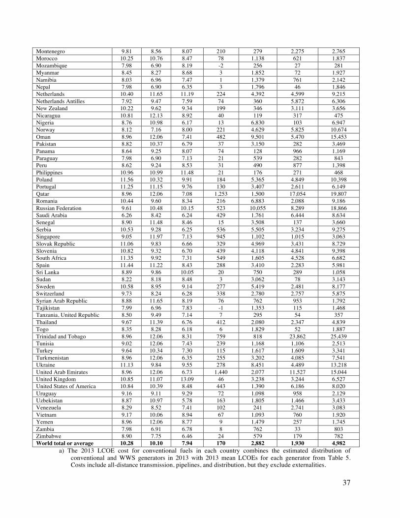
37

Montenegro 9.81 8.56 8.07 210 279 2,275 2,765 Morocco 10.25 10.76 8.47 78 1,138 621 1,837 Mozambique 7.98 6.90 8.19 -2 256 27 281 Myanmar 8.45 8.27 8.68 3 1,852 72 1,927 Namibia 8.03 6.96 7.47 1 1,379 761 2,142 Nepal 7.98 6.90 6.35 3 1,796 46 1,846 Netherlands 10.40 11.65 11.19 224 4,392 4,599 9,215 Netherlands Antilles 7.92 9.47 7.59 74 360 5,872 6,306 New Zealand 10.22 9.62 9.34 199 346 3,111 3,656 Nicaragua 10.81 12.13 8.92 40 119 317 475 Nigeria 8.76 10.98 6.17 13 6,830 103 6,947 Norway 8.12 7.16 8.00 221 4,629 5,825 10,674 Oman 8.96 12.06 7.41 482 9,501 5,470 15,453 Pakistan 8.82 10.37 6.79 37 3,150 282 3,469 Panama 8.64 9.25 8.07 74 128 966 1,169 Paraguay 7.98 6.90 7.13 21 539 282 843 Peru 8.62 9.24 8.53 31 490 877 1,398 Philippines 10.96 10.99 11.48 21 176 271 468 Poland 11.56 10.32 9.91 184 5,365 4,849 10,398 Portugal 11.25 11.15 9.76 130 3,407 2,611 6,149 Qatar 8.96 12.06 7.08 1,253 1,500 17,054 19,807 Romania 10.44 9.60 8.34 216 6,883 2,088 9,186 Russian Federation 9.61 10.48 10.15 523 10,055 8,289 18,866 Saudi Arabia 6.26 8.42 6.24 429 1,761 6,444 8,634 Senegal 8.90 11.48 8.46 15 3,508 137 3,660 Serbia 10.53 9.28 6.25 536 5,505 3,234 9,275 Singapore 9.05 11.97 7.13 945 1,102 1,015 3,063 Slovak Republic 11.06 9.83 6.66 329 4,969 3,431 8,729 Slovenia 10.82 9.32 6.70 439 4,118 4,841 9,398 South Africa 11.35 9.92 7.31 549 1,605 4,528 6,682 Spain 11.44 11.22 8.43 288 3,410 2,283 5,981 Sri Lanka 8.89 9.86 10.05 20 750 289 1,058 Sudan 8.22 8.18 8.48 3 3,062 78 3,143 Sweden 10.58 8.95 9.14 277 5,419 2,481 8,177 Switzerland 9.73 8.24 6.28 338 2,780 2,757 5,875 Syrian Arab Republic 8.88 11.65 8.19 76 762 953 1,792 Tajikistan 7.99 6.96 7.83 -1 1,353 115 1,468 Tanzania, United Republic 8.50 9.49 7.14 7 295 54 357 Thailand 9.67 11.39 6.76 412 2,080 2,347 4,839 Togo 8.35 8.28 6.18 6 1,829 52 1,887 Trinidad and Tobago 8.96 12.06 8.31 759 818 23,862 25,439 Tunisia 9.02 12.06 7.43 239 1,168 1,106 2,513 Turkey 9.64 10.34 7.30 115 1,617 1,609 3,341 Turkmenistan 8.96 12.06 6.35 255 3,202 4,085 7,541 Ukraine 11.13 9.84 9.55 278 8,451 4,489 13,218 United Arab Emirates 8.96 12.06 6.73 1,440 2,077 11,527 15,044 United Kingdom 10.85 11.07 13.09 46 3,238 3,244 6,527 United States of America 10.84 10.39 8.48 443 1,390 6,186 8,020 Uruguay 9.16 9.11 9.29 72 1,098 958 2,129 Uzbekistan 8.87 10.97 5.78 163 1,805 1,466 3,433 Venezuela 8.29 8.52 7.41 102 241 2,741 3,083 Vietnam 9.17 10.06 8.94 67 1,093 760 1,920 Yemen 8.96 12.06 8.77 9 1,479 257 1,745 Zambia 7.98 6.91 6.78 8 762 33 803 Zimbabwe 8.90 7.75 6.46 24 579 179 782 World total or average 10.28 10.10 7.94 170 2,882 1,930 4,982

a) The 2013 LCOE cost for conventional fuels in each country combines the estimated distribution of conventional and WWS generators in 2013 with 2013 mean LCOEs for each generator from Table 5. Costs include all-distance transmission, pipelines, and distribution, but they exclude externalities.

38

b) Same as (a), but for a 2050 BAU case (Supplemental Information) and 2050 LCOEs for each generator from Table 5. The 2050 BAU case includes significant existing WWS (mostly hydropower) plus future increases in WWS and energy efficiency.

c) The 2050 LCOE of WWS in the country combines the 2050 distribution of WWS generators from Table 3 with the 2050 mean LCOEs for each WWS generator from Table 5. The LCOE accounts for all-distance transmission and distribution (footnotes to Tables 2 and 5).

d) The total cost of electricity use in the electricity sector in the BAU (the product of electricity use and the LCOE) less the total cost in the electricity sector in the WWS scenario and less the annualized cost of the assumed efficiency improvements in the electricity sector in the WWS scenario. (See Delucchi et al., 2015 for details.)

e) Total cost of air pollution per year in the country from Table 7 divided by the 2050 population of the country.

f) Total climate cost per year to the world due to country’s emissions (Table 8) divided by the 2050 population of the country.

g) The sum of columns (d), (e), and (f). 8. Air Pollution and Global Warming Damage Costs Eliminated by WWS Conversion to a 100% WWS energy infrastructure in the 139 countries will eliminate energy-related air pollution mortality and morbidity and the associated health costs, and it will eliminate energy-related climate change costs to the world while causing variable climate impacts on individual countries. This section discusses these topics. 8.A. Air Pollution Cost Reductions due to WWS The benefits of reducing air pollution mortality and its costs in each U.S. country can be quantified as follows. First, the premature human mortality rate worldwide due to cardiovascular disease, respiratory disease, and complications from asthma arising from air pollution has been estimated previously by combining computer model estimates of human exposure to particulate matter (PM2.5) and ozone (O3) with the relative risk of mortality from these chemicals and population. Results are that an estimated 4-7 million people currently perish prematurely each year worldwide from outdoor plus indoor air pollution (e.g., Shindell et al., 2012; Anenberg et al., 2012; WHO, 2014; OECD, 2014). These mortalities represent ~0.7-1.2% of the 570 million deaths/year worldwide in 2015. Here, we combine modeled concentrations of PM2.5 and O3 in each of 139 countries with the relative risk of mortality as a function of concentration and with population in a health-effects equation (e.g., Jacobson, 2010) to estimate low, medium, and high mortalities due to PM2.5 and O3 by country, then extrapolate the results forward to 2050 while accounting for efficiencies that occur under the BAU scenario. Figure 10 shows the results. Premature mortalities in 2014, summed over the 139 countries are estimated for PM2.5 to be ~4.28 (1.19-7.56) million/yr, and those for O3, ~279,000 (140,000-417,000)/yr. The sum is ~4.56 (1.33-7.98) million premature mortalities/yr for PM2.5 plus O3, which is in the range of the previous literature estimates. Figure 10. Modeled worldwide (all countries, including the 139 discussed in this paper) (a) PM2.5 and (b) O3 premature mortalities in 2014 as estimated with GATOR-GCMOM (Jacobson, 2010), a 3-dimensional global computer model.

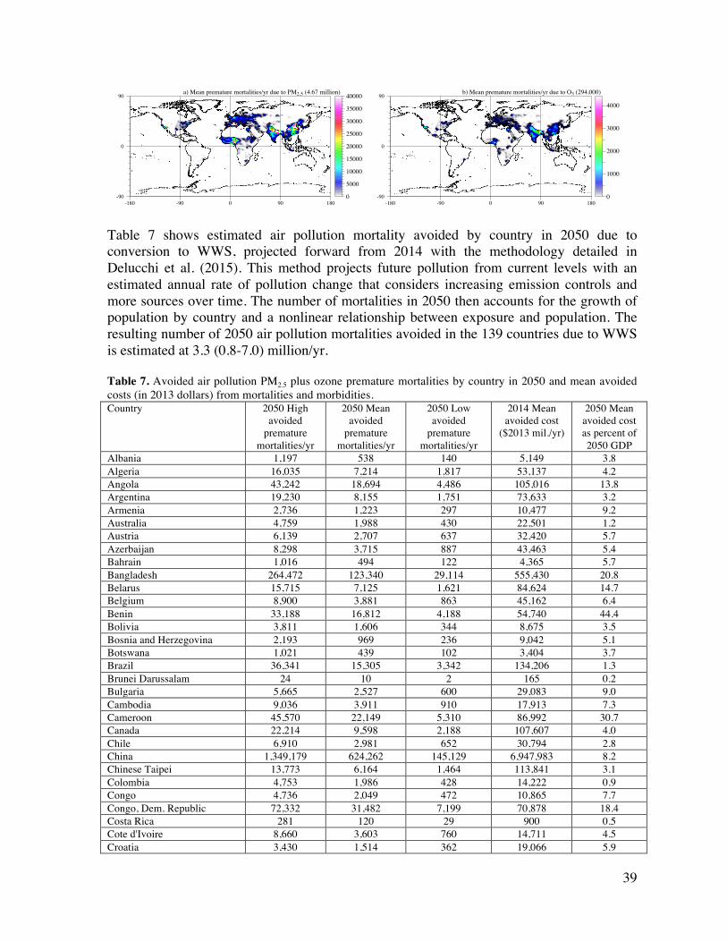
39

Table 7 shows estimated air pollution mortality avoided by country in 2050 due to conversion to WWS, projected forward from 2014 with the methodology detailed in Delucchi et al. (2015). This method projects future pollution from current levels with an estimated annual rate of pollution change that considers increasing emission controls and more sources over time. The number of mortalities in 2050 then accounts for the growth of population by country and a nonlinear relationship between exposure and population. The resulting number of 2050 air pollution mortalities avoided in the 139 countries due to WWS is estimated at 3.3 (0.8-7.0) million/yr. Table 7. Avoided air pollution PM2.5 plus ozone premature mortalities by country in 2050 and mean avoided costs (in 2013 dollars) from mortalities and morbidities. Country 2050 High

avoided premature

mortalities/yr

2050 Mean avoided

premature mortalities/yr

2050 Low avoided

premature mortalities/yr

2014 Mean avoided cost

($2013 mil./yr)

2050 Mean avoided cost as percent of 2050 GDP

Albania 1,197 538 140 5,149 3.8 Algeria 16,035 7,214 1,817 53,137 4.2 Angola 43,242 18,694 4,486 105,016 13.8 Argentina 19,230 8,155 1,751 73,633 3.2 Armenia 2,736 1,223 297 10,477 9.2 Australia 4,759 1,988 430 22,501 1.2 Austria 6,139 2,707 637 32,420 5.7 Azerbaijan 8,298 3,715 887 43,463 5.4 Bahrain 1,016 494 122 4,365 5.7 Bangladesh 264,472 123,340 29,114 555,430 20.8 Belarus 15,715 7,125 1,621 84,624 14.7 Belgium 8,900 3,881 863 45,162 6.4 Benin 33,188 16,812 4,188 54,740 44.4 Bolivia 3,811 1,606 344 8,675 3.5 Bosnia and Herzegovina 2,193 969 236 9,042 5.1 Botswana 1,021 439 102 3,404 3.7 Brazil 36,341 15,305 3,342 134,206 1.3 Brunei Darussalam 24 10 2 165 0.2 Bulgaria 5,665 2,527 600 29,083 9.0 Cambodia 9,036 3,911 910 17,913 7.3 Cameroon 45,570 22,149 5,310 86,992 30.7 Canada 22,214 9,598 2,188 107,607 4.0 Chile 6,910 2,981 652 30,794 2.8 China 1,349,179 624,262 145,129 6,947,983 8.2 Chinese Taipei 13,773 6,164 1,464 113,841 3.1 Colombia 4,753 1,986 428 14,222 0.9 Congo 4,736 2,049 472 10,865 7.7 Congo, Dem. Republic 72,332 31,482 7,199 70,878 18.4 Costa Rica 281 120 29 900 0.5 Cote d'Ivoire 8,660 3,603 760 14,711 4.5 Croatia 3,430 1,514 362 19,066 5.9

a) Mean premature mortalities/yr due to PM2.5 (4.67 million)

0

5000

10000

15000

20000

25000

30000

35000

40000

-180 -90 0 90 180-90

0

90b) Mean premature mortalities/yr due to O3 (294,000)

0

1000

2000

3000

4000

-180 -90 0 90 180-90

0

90

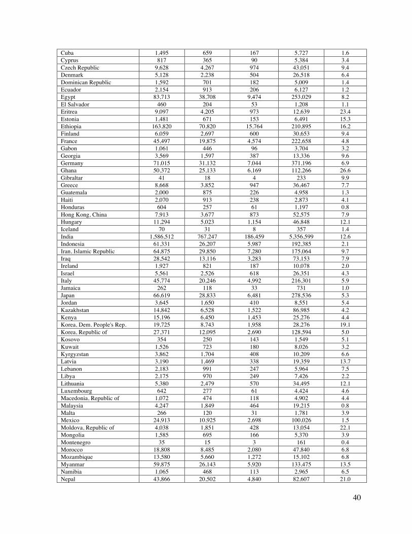
40

Cuba 1,495 659 167 5,727 1.6 Cyprus 817 365 90 5,384 3.4 Czech Republic 9,628 4,267 974 43,051 9.4 Denmark 5,128 2,238 504 26,518 6.4 Dominican Republic 1,592 701 182 5,009 1.4 Ecuador 2,154 913 206 6,127 1.2 Egypt 83,713 38,708 9,474 253,029 8.2 El Salvador 460 204 53 1,208 1.1 Eritrea 9,097 4,205 973 12,639 23.4 Estonia 1,481 671 153 6,491 15.3 Ethiopia 163,820 70,820 15,764 210,895 16.2 Finland 6,059 2,697 600 30,653 9.4 France 45,497 19,875 4,574 222,658 4.8 Gabon 1,061 446 96 3,704 3.2 Georgia 3,569 1,597 387 13,336 9.6 Germany 71,015 31,132 7,044 371,196 6.9 Ghana 50,372 25,133 6,169 112,266 26.6 Gibraltar 41 18 4 233 9.9 Greece 8,668 3,852 947 36,467 7.7 Guatemala 2,000 875 226 4,958 1.3 Haiti 2,070 913 238 2,873 4.1 Honduras 604 257 61 1,197 0.8 Hong Kong, China 7,913 3,677 873 52,575 7.9 Hungary 11,294 5,023 1,154 46,848 12.1 Iceland 70 31 8 357 1.4 India 1,586,512 767,247 186,459 5,356,599 12.6 Indonesia 61,331 26,207 5,987 192,385 2.1 Iran, Islamic Republic 64,875 29,850 7,280 175,064 9.7 Iraq 28,542 13,116 3,283 73,153 7.9 Ireland 1,927 821 187 10,078 2.0 Israel 5,561 2,526 618 26,351 4.3 Italy 45,774 20,246 4,992 216,301 5.9 Jamaica 262 118 33 731 1.0 Japan 66,619 28,833 6,481 278,536 5.3 Jordan 3,645 1,650 410 8,551 5.4 Kazakhstan 14,842 6,528 1,522 86,985 4.2 Kenya 15,196 6,450 1,453 25,276 4.4 Korea, Dem. People's Rep. 19,725 8,743 1,958 28,276 19.1 Korea, Republic of 27,371 12,095 2,690 128,594 5.0 Kosovo 354 250 143 1,549 5.1 Kuwait 1,526 723 180 8,026 3.2 Kyrgyzstan 3,862 1,704 408 10,209 6.6 Latvia 3,190 1,469 338 19,359 13.7 Lebanon 2,183 991 247 5,964 7.5 Libya 2,175 970 249 7,426 2.2 Lithuania 5,380 2,479 570 34,495 12.1 Luxembourg 642 277 61 4,424 4.6 Macedonia, Republic of 1,072 474 118 4,902 4.4 Malaysia 4,247 1,849 464 19,215 0.8 Malta 266 120 31 1,781 3.9 Mexico 24,913 10,925 2,698 100,026 1.5 Moldova, Republic of 4,038 1,851 428 13,054 22.1 Mongolia 1,585 695 166 5,370 3.9 Montenegro 35 15 3 161 0.4 Morocco 18,808 8,485 2,080 47,840 6.8 Mozambique 13,580 5,660 1,272 15,102 6.8 Myanmar 59,875 26,143 5,920 133,475 13.5 Namibia 1,065 468 113 2,965 6.5 Nepal 43,866 20,502 4,840 82,607 21.0

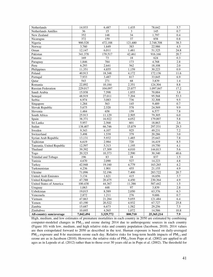
41

Netherlands 14,933 6,487 1,435 78,642 5.7 Netherlands Antilles 36 15 3 145 0.7 New Zealand 352 148 34 1,797 0.4 Nicaragua 372 159 37 858 0.8 Nigeria 900,528 472,188 121,680 2,748,708 38.3 Norway 3,760 1,649 383 22,986 4.5 Oman 12,147 6,011 1,481 51,325 24.8 Pakistan 341,378 170,517 42,461 916,166 20.7 Panama 169 73 18 624 0.3 Paraguay 1,846 784 173 4,768 2.8 Peru 6,293 2,641 562 18,108 2.0 Philippines 11,351 4,855 1,159 30,223 0.9 Poland 40,913 18,348 4,172 172,136 11.6 Portugal 7,933 3,487 817 33,845 6.9 Qatar 543 271 68 3,839 1.4 Romania 22,892 10,184 2,351 124,304 8.8 Russian Federation 229,017 104,097 23,877 1,097,847 17.2 Saudi Arabia 15,938 7,598 1,855 70,884 3.8 Senegal 48,919 27,011 7,204 95,568 53.3 Serbia 6,974 3,083 736 32,308 9.5 Singapore 1,284 563 145 9,489 0.7 Slovak Republic 5,675 2,520 578 24,569 9.9 Slovenia 1,484 658 159 6,577 7.8 South Africa 25,913 11,129 2,505 79,305 6.0 Spain 38,371 16,922 4,052 179,007 5.8 Sri Lanka 5,957 2,568 601 18,863 2.6 Sudan 138,407 66,746 15,879 297,531 29.3 Sweden 9,343 4,107 925 49,231 7.2 Switzerland 3,498 1,539 379 20,286 3.0 Syrian Arab Republic 13,131 5,932 1,485 25,643 7.8 Tajikistan 6,619 2,984 720 16,419 8.5 Tanzania, United Republic 12,597 5,313 1,195 19,750 4.1 Thailand 39,392 17,309 4,010 144,813 5.6 Togo 20,323 10,373 2,590 30,340 40.6 Trinidad and Tobago 196 83 18 837 1.5 Tunisia 4,670 2,090 527 14,223 4.8 Turkey 42,948 19,160 4,779 163,265 4.2 Turkmenistan 4,236 1,901 455 21,155 4.9 Ukraine 71,096 32,196 7,400 283,722 20.7 United Arab Emirates 3,134 1,621 415 16,656 3.7 United Kingdom 47,788 20,475 4,450 230,364 4.9 United States of America 100,438 44,367 11,386 587,442 1.5 Uruguay 1,063 448 97 3,839 2.8 Uzbekistan 19,015 8,589 2,050 63,376 6.3 Venezuela 2,872 1,211 276 9,686 0.7 Vietnam 47,863 21,284 5,055 121,484 6.4 Yemen 43,190 20,522 4,932 67,727 25.8 Zambia 15,687 6,673 1,582 29,256 7.5 Zimbabwe 10,695 4,565 1,072 14,586 10.8 All-country sum/average 7,042,494 3,329,772 800,710 25,365,214 7.9 High, medium, and low estimates of premature mortalities in each country in 2050 are estimated by combining computer-modeled changes in PM2.5 and ozone during 2014 due to anthropogenic sources in each country (Figure 10) with low, medium, and high relative risks and country population (Jacobson, 2010). 2014 values are then extrapolated forward to 2050 as described in the text. Human exposure is based on daily-averaged PM2.5 exposure and 8-hr maximum ozone each day. Relative risks for long-term health impacts of PM2.5 and ozone are as in Jacobson (2010). However, the relative risks of PM2.5 from Pope et al. (2002) are applied to all ages as in Lepeule et al. (2012) rather than to those over 30 years old as in Pope et al. (2002). The threshold for

42

PM2.5 is zero but concentrations below 8 µg/m3 are down-weighted as in Jacobson (2010). The low ambient concentration threshold for ozone premature mortality is assumed to be 35 ppbv. Air pollution costs are estimated by multiplying the value of statistical life (VSL) in each country by the low, medium, and high number of excess mortalities due to PM2.5 and ozone. Estimates of the VSL are calculated as in Delucchi et al. (2015). Values for the U.S. are projected to 2050 based on GDP per capita projections (on a PPP basis) for the U.S. then scaled by country as a nonlinear function of GDP per capita in each country to the U.S. Multipliers are then used to account for morbidity and non-health impacts of air pollution. Cost of air pollution. The total damage cost of air pollution due to conventional fuels (fossil fuel and biofuel combustion and evaporative emissions) in a country is the sum of mortality costs, morbidity costs, and non-health costs such as lost visibility and agricultural output in the country. The mortality cost equals the number of mortalities in the country multiplied by the value of statistical life (VSL). The methodology for determining the VSL by country is provided in the footnote to Table 7. The morbidity plus non-health cost per country is estimated as the mortality cost multiplied by the ratio of the value of total air-pollution damages (mortality plus morbidity plus other damages) to mortality costs alone. The result of the calculation is that the 139-country cost of air pollution in 2050 is ~$25.4 ($4.3-$69.7) trillion/yr, which corresponds to ~7.9 (1.3-21.6)% of 2050 global annual GDP on a PPP basis. 8.B. Global-Warming Damage Costs Eliminated by 100% WWS in Each Country This section provides estimates of two kinds of climate change costs due to greenhouse gas (GHG) emissions from energy use (Table 8). GHG emissions are defined here to include emissions of carbon dioxide, other greenhouse gases, and air pollution particles that cause global warming, converted to equivalent carbon dioxide. A 100% WWS system in each country will eliminate such damages. The cost calculated is the cost of climate change impacts to the world attributable to emissions of GHGs from each country. Costs of climate change include coastal flood and real estate damage costs, agricultural loss costs, energy-sector costs, water costs, health costs due to heat stress and heat stroke, influenza and malaria costs, famine costs, ocean acidification costs, increased drought and wildfire costs, severe weather costs, and increased air pollution health costs. These costs are partly offset by fewer extreme cold events and associated reductions in illnesses and mortalities and gains in agriculture in some regions. Net costs due to global-warming-relevant emissions are embodied in the social cost of carbon dioxide. The range of the 2050 social cost of carbon from recent papers is $500 (282-1,063)/metric tonne-CO2e in 2013 dollars (Jacobson et al., 2015a). This range is used to derive the costs in Table 8. Table 8. Percent of 2013 world CO2 emissions by country (GCP, 2014) and low, medium, and high estimates of avoided 2050 global climate-change costs due to converting each country to 100% WWS for all purposes. All costs are in 2013 dollars. 2013 2050 avoided global climate cost ($2013 bil./yr) Country Percent of world

CO2 emissions Low Medium High

Albania 0.014 4.9 2.3 1.3 Algeria 0.419 152.1 71.4 40.3 Angola 0.092 33.2 15.6 8.8 Argentina 0.577 209.3 98.3 55.4 Armenia 0.012 4.2 2.0 1.1

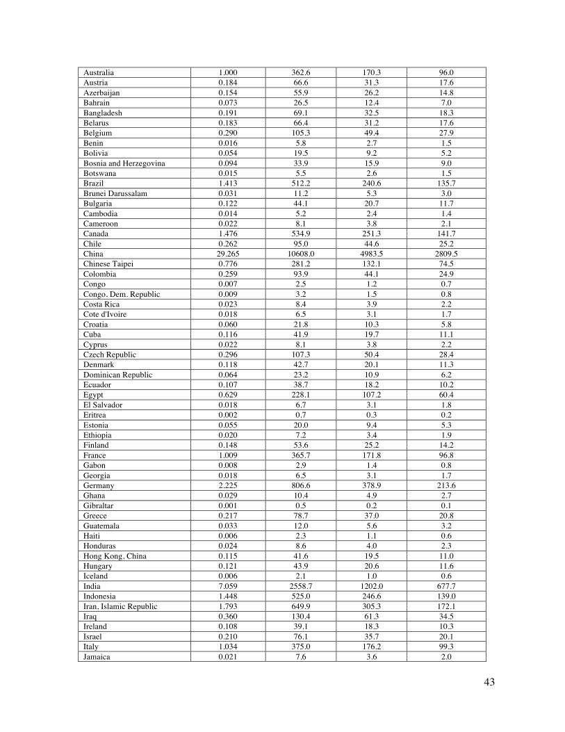
43

Australia 1.000 362.6 170.3 96.0 Austria 0.184 66.6 31.3 17.6 Azerbaijan 0.154 55.9 26.2 14.8 Bahrain 0.073 26.5 12.4 7.0 Bangladesh 0.191 69.1 32.5 18.3 Belarus 0.183 66.4 31.2 17.6 Belgium 0.290 105.3 49.4 27.9 Benin 0.016 5.8 2.7 1.5 Bolivia 0.054 19.5 9.2 5.2 Bosnia and Herzegovina 0.094 33.9 15.9 9.0 Botswana 0.015 5.5 2.6 1.5 Brazil 1.413 512.2 240.6 135.7 Brunei Darussalam 0.031 11.2 5.3 3.0 Bulgaria 0.122 44.1 20.7 11.7 Cambodia 0.014 5.2 2.4 1.4 Cameroon 0.022 8.1 3.8 2.1 Canada 1.476 534.9 251.3 141.7 Chile 0.262 95.0 44.6 25.2 China 29.265 10608.0 4983.5 2809.5 Chinese Taipei 0.776 281.2 132.1 74.5 Colombia 0.259 93.9 44.1 24.9 Congo 0.007 2.5 1.2 0.7 Congo, Dem. Republic 0.009 3.2 1.5 0.8 Costa Rica 0.023 8.4 3.9 2.2 Cote d'Ivoire 0.018 6.5 3.1 1.7 Croatia 0.060 21.8 10.3 5.8 Cuba 0.116 41.9 19.7 11.1 Cyprus 0.022 8.1 3.8 2.2 Czech Republic 0.296 107.3 50.4 28.4 Denmark 0.118 42.7 20.1 11.3 Dominican Republic 0.064 23.2 10.9 6.2 Ecuador 0.107 38.7 18.2 10.2 Egypt 0.629 228.1 107.2 60.4 El Salvador 0.018 6.7 3.1 1.8 Eritrea 0.002 0.7 0.3 0.2 Estonia 0.055 20.0 9.4 5.3 Ethiopia 0.020 7.2 3.4 1.9 Finland 0.148 53.6 25.2 14.2 France 1.009 365.7 171.8 96.8 Gabon 0.008 2.9 1.4 0.8 Georgia 0.018 6.5 3.1 1.7 Germany 2.225 806.6 378.9 213.6 Ghana 0.029 10.4 4.9 2.7 Gibraltar 0.001 0.5 0.2 0.1 Greece 0.217 78.7 37.0 20.8 Guatemala 0.033 12.0 5.6 3.2 Haiti 0.006 2.3 1.1 0.6 Honduras 0.024 8.6 4.0 2.3 Hong Kong, China 0.115 41.6 19.5 11.0 Hungary 0.121 43.9 20.6 11.6 Iceland 0.006 2.1 1.0 0.6 India 7.059 2558.7 1202.0 677.7 Indonesia 1.448 525.0 246.6 139.0 Iran, Islamic Republic 1.793 649.9 305.3 172.1 Iraq 0.360 130.4 61.3 34.5 Ireland 0.108 39.1 18.3 10.3 Israel 0.210 76.1 35.7 20.1 Italy 1.034 375.0 176.2 99.3 Jamaica 0.021 7.6 3.6 2.0

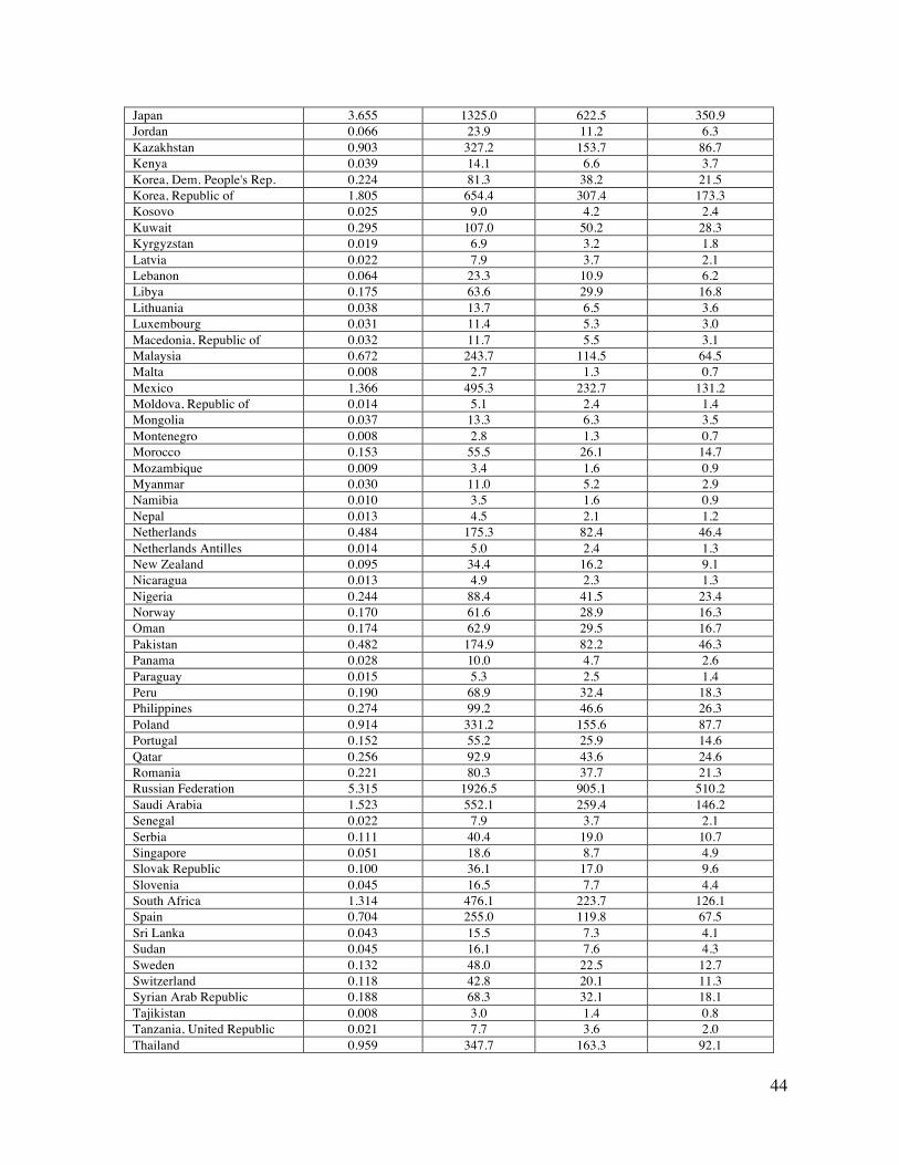
44

Japan 3.655 1325.0 622.5 350.9 Jordan 0.066 23.9 11.2 6.3 Kazakhstan 0.903 327.2 153.7 86.7 Kenya 0.039 14.1 6.6 3.7 Korea, Dem. People's Rep. 0.224 81.3 38.2 21.5 Korea, Republic of 1.805 654.4 307.4 173.3 Kosovo 0.025 9.0 4.2 2.4 Kuwait 0.295 107.0 50.2 28.3 Kyrgyzstan 0.019 6.9 3.2 1.8 Latvia 0.022 7.9 3.7 2.1 Lebanon 0.064 23.3 10.9 6.2 Libya 0.175 63.6 29.9 16.8 Lithuania 0.038 13.7 6.5 3.6 Luxembourg 0.031 11.4 5.3 3.0 Macedonia, Republic of 0.032 11.7 5.5 3.1 Malaysia 0.672 243.7 114.5 64.5 Malta 0.008 2.7 1.3 0.7 Mexico 1.366 495.3 232.7 131.2 Moldova, Republic of 0.014 5.1 2.4 1.4 Mongolia 0.037 13.3 6.3 3.5 Montenegro 0.008 2.8 1.3 0.7 Morocco 0.153 55.5 26.1 14.7 Mozambique 0.009 3.4 1.6 0.9 Myanmar 0.030 11.0 5.2 2.9 Namibia 0.010 3.5 1.6 0.9 Nepal 0.013 4.5 2.1 1.2 Netherlands 0.484 175.3 82.4 46.4 Netherlands Antilles 0.014 5.0 2.4 1.3 New Zealand 0.095 34.4 16.2 9.1 Nicaragua 0.013 4.9 2.3 1.3 Nigeria 0.244 88.4 41.5 23.4 Norway 0.170 61.6 28.9 16.3 Oman 0.174 62.9 29.5 16.7 Pakistan 0.482 174.9 82.2 46.3 Panama 0.028 10.0 4.7 2.6 Paraguay 0.015 5.3 2.5 1.4 Peru 0.190 68.9 32.4 18.3 Philippines 0.274 99.2 46.6 26.3 Poland 0.914 331.2 155.6 87.7 Portugal 0.152 55.2 25.9 14.6 Qatar 0.256 92.9 43.6 24.6 Romania 0.221 80.3 37.7 21.3 Russian Federation 5.315 1926.5 905.1 510.2 Saudi Arabia 1.523 552.1 259.4 146.2 Senegal 0.022 7.9 3.7 2.1 Serbia 0.111 40.4 19.0 10.7 Singapore 0.051 18.6 8.7 4.9 Slovak Republic 0.100 36.1 17.0 9.6 Slovenia 0.045 16.5 7.7 4.4 South Africa 1.314 476.1 223.7 126.1 Spain 0.704 255.0 119.8 67.5 Sri Lanka 0.043 15.5 7.3 4.1 Sudan 0.045 16.1 7.6 4.3 Sweden 0.132 48.0 22.5 12.7 Switzerland 0.118 42.8 20.1 11.3 Syrian Arab Republic 0.188 68.3 32.1 18.1 Tajikistan 0.008 3.0 1.4 0.8 Tanzania, United Republic 0.021 7.7 3.6 2.0 Thailand 0.959 347.7 163.3 92.1

45

Togo 0.005 1.8 0.9 0.5 Trinidad and Tobago 0.143 52.0 24.4 13.8 Tunisia 0.079 28.7 13.5 7.6 Turkey 0.954 345.7 162.4 91.6 Turkmenistan 0.158 57.4 27.0 15.2 Ukraine 0.885 320.8 150.7 85.0 United Arab Emirates 0.543 196.8 92.4 52.1 United Kingdom 1.355 491.3 230.8 130.1 United States of America 15.350 5564.1 2614.0 1473.6 Uruguay 0.020 7.1 3.3 1.9 Uzbekistan 0.302 109.5 51.5 29.0 Venezuela 0.648 234.9 110.3 62.2 Vietnam 0.496 179.9 84.5 47.7 Yemen 0.069 25.0 11.8 6.6 Zambia 0.007 2.7 1.3 0.7 Zimbabwe 0.027 9.6 4.5 2.5 World total or average 99.747 36,156 16,986 9,576 Table 8 indicates that the sum of the 139-country greenhouse gas and particle emissions may cause, in 2050, $17 (9.6-36) trillion/year in climate damage to the world. Thus, the global climate cost savings per person, averaged among these countries, to reducing all climate-relevant emissions through a 100% WWS system, is ~$2,520/person/year (in 2013 dollars) (Table 6). 9. Impacts of WWS on Jobs and Earnings in the Energy Power Sector. This section provides estimates of job and revenue creation and loss due to implementing WWS electricity. The analysis does not include the job changes in industries outside of electric power generation, such as in the manufacture of electric vehicles, fuel cells or electricity storage because of the additional complexity required and greater uncertainty as to where those jobs will be located. 9.A. JEDI Job Creation Analysis Changes in jobs and total earnings are estimated here first with the Jobs and Economic Development Impact (JEDI) models (NREL, 2013). These are economic input-output models with several assumptions and uncertainties (e.g. Linowes, 2012). They incorporate three levels of impacts: 1) project development and onsite labor impacts; 2) local revenue and supply chain impacts; and 3) induced impacts. Jobs and revenue are reported for two phases of development: 1) the construction period and 2) operating years. Scenarios for WWS powered electricity generation are run for each country assuming that the WWS electricity sector is fully developed by 2050. The calculations account for only new WWS jobs associated with new WWS generator capacity as identified in Table 2 and corresponding new transmission lines. As construction jobs are temporary in nature, JEDI models report construction job creation as full-time equivalents (FTE, equal to 2,080 hours of work per year). We assume for the jobs calculation that each year from 2015 to 2050, 1/35th of the WWS infrastructure is built. The number of jobs associated with new transmission lines assumes 80% of new lines will be 500 kV high-voltage direct current (HVDC) lines and 20% 230 kV alternating current (AC) lines. Total line length is simplistically assumed to equal five times the circular radius

46

of a country. The transmission line JEDI model is used to calculate construction FTE jobs and annual operations jobs for the 230 kV AC lines for each country. For HVDC lines, the actual average numbers of construction FTE jobs and annual operation jobs among five proposed projects in the U.S. (Clean Line Energy Partners, 2016) are multiplied by the ratio of JEDI-model predicted number of jobs in a given country to that in the U.S. assuming 500 kV HVDC lines. Table 9. Estimated new 35-year construction jobs, new 35-year operation jobs, 35-year construction plus operation jobs minus jobs lost, annual earnings corresponding to new construction and operation jobs, and net earnings from new construction plus operation jobs minus jobs lost (current jobs plus future jobs lost due to not growing fossil-fuel infrastructure), by country, due to converting to 100% WWS, based on the number of new generators needed of each type for annual average power and peaking/storage (Table 2). Earnings include wages, services, and supply-chain impacts.

Country 35-year construction

jobs

35-year operation

jobs

Job losses in fossil-fuel

and nuclear energy

industries

35-year net construction

plus operation

jobs created minus jobs

lost

Annual earnings from

new 40-year

construction jobs (bil

2013-$/ yr)

Earnings from

new 40-year

operation jobs

(bil 2013-$/yr)

Net earnings from new

construct-ion plus operation

jobs minus jobs lost

(bil 2013-$/yr)

Albania 6,187 6,133 6,619 5,700 0.31 0.47 0.29 Algeria 132,730 131,815 328,769 (64,224) 5.64 7.07 -4.57 Angola 31,697 17,825 274,881 (225,360) 0.95 0.69 -9.01 Argentina 117,016 115,046 171,709 60,354 6.64 8.06 2.98 Armenia 6,771 7,186 4,213 9,744 0.29 0.47 0.52 Australia 160,274 253,941 212,231 201,984 12.82 24.61 17.17 Austria 66,180 96,174 38,847 123,507 5.72 10.16 11.89 Azerbaijan 22,283 22,671 83,443 (38,488) 1.49 2.31 -4.58 Bahrain 13,458 18,340 44,380 (12,582) 0.93 1.25 -0.85 Bangladesh 128,102 98,072 205,298 20,877 2.82 3.02 -0.17 Belarus 96,367 129,650 35,672 190,345 6.58 13.52 16.55 Belgium 138,494 230,177 40,724 327,947 11.42 23.26 30.69 Benin 7,680 6,990 40,413 (25,743) 0.13 0.16 -0.63 Bolivia 17,276 12,482 49,459 (19,701) 0.50 0.47 -0.86 Bosnia and Herzegovina 11,005 10,795 9,434 12,366 0.52 0.79 0.69 Botswana 6,154 7,728 6,320 7,562 0.28 0.44 0.36 Brazil 805,170 773,637 999,444 579,364 39.37 52.11 28.67 Brunei Darussalam 5,634 7,021 29,350 (16,694) 0.79 1.23 -3.08 Bulgaria 40,203 52,452 27,158 65,498 2.61 5.21 5.37 Cambodia 13,708 8,746 46,227 (23,773) 0.31 0.27 -0.85 Cameroon 16,725 16,243 85,257 (52,289) 0.34 0.44 -1.47 Canada 292,986 463,322 580,544 175,765 23.40 44.28 13.67 Chile 87,315 119,086 118,784 87,617 5.42 10.09 6.17 China 6,695,881 6,492,101 4,175,098 9,012,884 425.66 613.69 681.99 Chinese Taipei 257,718 165,443 130,932 292,229 39.41 36.13 51.51 Colombia 68,993 78,200 161,054 (13,861) 2.82 4.05 -1.33 Congo 4,026 3,331 57,148 (49,791) 0.11 0.12 -1.84 Congo, Dem. Republic 69,678 69,145 510,596 (371,773) 0.87 1.17 -6.50 Costa Rica 8,373 5,151 10,603 2,922 0.36 0.28 0.09 Cote d'Ivoire 20,346 19,054 127,848 (88,449) 0.43 0.53 -2.56 Croatia 21,457 31,025 15,622 36,860 1.61 3.54 3.43 Cuba 20,219 19,151 19,483 19,887 1.08 1.27 1.11 Cyprus 5,366 6,247 2,873 8,740 0.52 0.92 1.06

47

Czech Republic 74,716 81,158 37,396 118,479 4.90 6.65 8.60 Denmark 18,552 31,663 32,560 17,654 1.58 3.29 1.53 Dominican Republic 14,202 7,540 14,363 7,380 0.58 0.39 0.27 Ecuador 24,209 19,155 66,306 (22,942) 0.91 0.92 -1.29 Egypt 200,576 174,629 341,151 34,053 7.28 8.10 0.47 El Salvador 6,218 3,516 10,329 (595) 0.20 0.15 -0.07 Eritrea 2,006 1,172 13,576 (10,397) 0.03 0.02 -0.23 Estonia 4,450 6,245 7,370 3,325 0.27 0.48 0.21 Ethiopia 89,505 60,372 633,140 (483,263) 1.41 1.27 -10.57 Finland 47,316 82,222 38,261 91,277 3.75 8.02 8.15 France 320,178 329,457 173,156 476,479 24.80 31.45 40.44 Gabon 7,377 10,216 36,164 (18,571) 0.37 0.64 -1.23 Georgia 8,663 9,003 8,403 9,263 0.35 0.57 0.44 Germany 786,658 1,203,675 229,418 1,760,914 67.56 126.27 170.58 Ghana 23,965 23,005 76,632 (29,661) 0.56 0.70 -1.00 Gibraltar 2,884 3,179 1,651 4,412 0.28 0.36 0.46 Greece 32,152 29,511 26,081 35,582 1.91 2.21 2.25 Guatemala 21,538 11,805 45,431 (12,089) 0.65 0.46 -0.64 Haiti 5,903 3,670 35,591 (26,019) 0.10 0.08 -0.60 Honduras 10,167 7,760 22,133 (4,206) 0.25 0.25 -0.19 Hong Kong, China 63,420 88,748 28,433 123,735 6.94 12.43 15.81 Hungary 57,634 61,612 24,034 95,212 3.35 4.52 6.15 Iceland 1,277 3,125 3,770 632 0.11 0.32 0.07 India 1,905,892 1,698,048 2,508,442 1,095,497 66.46 85.26 34.89 Indonesia 542,376 500,691 812,101 230,966 21.18 26.76 5.74 Iran, Islamic Republic 428,126 505,881 758,697 175,310 16.35 20.67 6.19 Iraq 56,028 57,091 333,803 (220,684) 2.00 2.20 -8.63 Ireland 11,375 16,049 10,844 16,579 1.03 1.76 1.64 Israel 35,321 37,484 18,138 54,667 2.44 3.22 4.20 Italy 367,618 510,080 133,351 744,347 26.37 45.39 60.28 Jamaica 5,666 4,756 6,159 4,263 0.19 0.21 0.14 Japan 609,972 775,535 216,731 1,168,776 42.28 59.71 85.73 Jordan 11,438 11,082 16,051 6,468 0.37 0.39 0.21 Kazakhstan 133,237 186,358 198,466 121,129 10.97 23.28 9.98 Kenya 33,780 23,761 184,209 (126,668) 0.68 0.64 -3.56 Korea, Dem. People's Rep. 60,011 89,493 80,135 69,369 1.01 2.02 1.35 Korea, Republic of 554,236 696,549 218,433 1,032,352 40.61 61.54 84.24 Kosovo 4,499 3,927 6,163 2,263 0.15 0.17 0.07 Kuwait 41,772 61,753 230,457 (126,932) 4.21 5.81 -11.74 Kyrgyzstan 12,599 11,926 11,264 13,261 0.34 0.50 0.42 Latvia 13,249 21,899 14,758 20,390 1.07 2.69 1.99 Lebanon 12,090 15,144 12,802 14,433 0.48 0.64 0.59 Libya 28,804 36,810 189,158 (123,544) 1.29 2.07 -7.08 Lithuania 15,343 22,630 12,922 25,050 1.36 3.03 2.69 Luxembourg 10,474 13,682 3,153 21,003 1.52 2.32 3.31 Macedonia, Republic of 6,642 6,964 4,597 9,009 0.37 0.59 0.60 Malaysia 201,726 249,037 242,179 208,584 12.97 21.29 14.59 Malta 4,416 7,730 2,271 9,875 0.44 1.16 1.27 Mexico 357,982 276,549 681,535 (47,004) 18.55 19.76 -7.89 Moldova, Republic of 7,506 7,904 6,329 9,081 0.25 0.40 0.35 Mongolia 14,981 18,296 20,772 12,506 0.63 1.04 0.53 Montenegro 1,862 2,302 2,655 1,509 0.11 0.21 0.10 Morocco 50,417 47,700 50,580 47,538 1.52 1.86 1.58 Mozambique 20,054 17,820 235,785 (197,911) 0.29 0.34 -3.77 Myanmar 47,164 44,916 132,282 (40,202) 1.19 1.57 -1.80 Namibia 6,297 8,612 40,507 (25,597) 0.22 0.38 -1.19 Nepal 29,159 25,110 89,848 (35,579) 0.57 0.69 -1.18 Netherlands 130,655 202,498 104,308 228,844 11.54 21.80 22.27 Netherlands Antilles 5,867 6,931 4,992 7,806 0.36 0.53 0.51

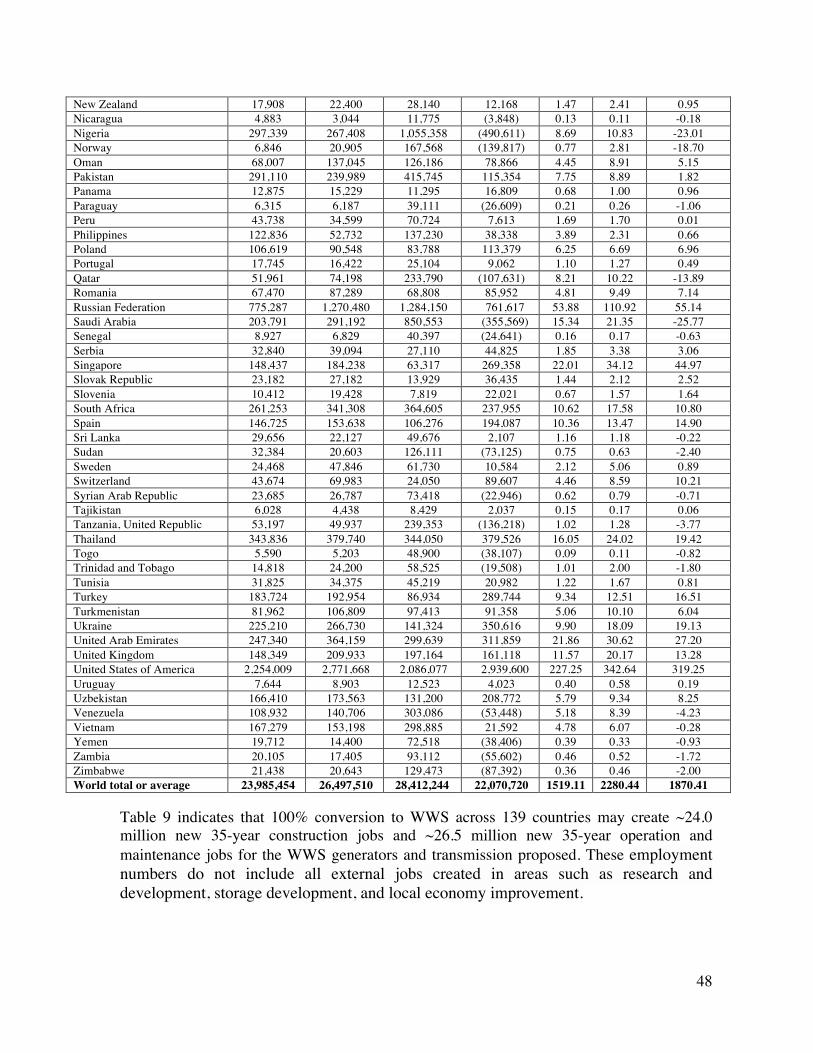
48

New Zealand 17,908 22,400 28,140 12,168 1.47 2.41 0.95 Nicaragua 4,883 3,044 11,775 (3,848) 0.13 0.11 -0.18 Nigeria 297,339 267,408 1,055,358 (490,611) 8.69 10.83 -23.01 Norway 6,846 20,905 167,568 (139,817) 0.77 2.81 -18.70 Oman 68,007 137,045 126,186 78,866 4.45 8.91 5.15 Pakistan 291,110 239,989 415,745 115,354 7.75 8.89 1.82 Panama 12,875 15,229 11,295 16,809 0.68 1.00 0.96 Paraguay 6,315 6,187 39,111 (26,609) 0.21 0.26 -1.06 Peru 43,738 34,599 70,724 7,613 1.69 1.70 0.01 Philippines 122,836 52,732 137,230 38,338 3.89 2.31 0.66 Poland 106,619 90,548 83,788 113,379 6.25 6.69 6.96 Portugal 17,745 16,422 25,104 9,062 1.10 1.27 0.49 Qatar 51,961 74,198 233,790 (107,631) 8.21 10.22 -13.89 Romania 67,470 87,289 68,808 85,952 4.81 9.49 7.14 Russian Federation 775,287 1,270,480 1,284,150 761,617 53.88 110.92 55.14 Saudi Arabia 203,791 291,192 850,553 (355,569) 15.34 21.35 -25.77 Senegal 8,927 6,829 40,397 (24,641) 0.16 0.17 -0.63 Serbia 32,840 39,094 27,110 44,825 1.85 3.38 3.06 Singapore 148,437 184,238 63,317 269,358 22.01 34.12 44.97 Slovak Republic 23,182 27,182 13,929 36,435 1.44 2.12 2.52 Slovenia 10,412 19,428 7,819 22,021 0.67 1.57 1.64 South Africa 261,253 341,308 364,605 237,955 10.62 17.58 10.80 Spain 146,725 153,638 106,276 194,087 10.36 13.47 14.90 Sri Lanka 29,656 22,127 49,676 2,107 1.16 1.18 -0.22 Sudan 32,384 20,603 126,111 (73,125) 0.75 0.63 -2.40 Sweden 24,468 47,846 61,730 10,584 2.12 5.06 0.89 Switzerland 43,674 69,983 24,050 89,607 4.46 8.59 10.21 Syrian Arab Republic 23,685 26,787 73,418 (22,946) 0.62 0.79 -0.71 Tajikistan 6,028 4,438 8,429 2,037 0.15 0.17 0.06 Tanzania, United Republic 53,197 49,937 239,353 (136,218) 1.02 1.28 -3.77 Thailand 343,836 379,740 344,050 379,526 16.05 24.02 19.42 Togo 5,590 5,203 48,900 (38,107) 0.09 0.11 -0.82 Trinidad and Tobago 14,818 24,200 58,525 (19,508) 1.01 2.00 -1.80 Tunisia 31,825 34,375 45,219 20,982 1.22 1.67 0.81 Turkey 183,724 192,954 86,934 289,744 9.34 12.51 16.51 Turkmenistan 81,962 106,809 97,413 91,358 5.06 10.10 6.04 Ukraine 225,210 266,730 141,324 350,616 9.90 18.09 19.13 United Arab Emirates 247,340 364,159 299,639 311,859 21.86 30.62 27.20 United Kingdom 148,349 209,933 197,164 161,118 11.57 20.17 13.28 United States of America 2,254,009 2,771,668 2,086,077 2,939,600 227.25 342.64 319.25 Uruguay 7,644 8,903 12,523 4,023 0.40 0.58 0.19 Uzbekistan 166,410 173,563 131,200 208,772 5.79 9.34 8.25 Venezuela 108,932 140,706 303,086 (53,448) 5.18 8.39 -4.23 Vietnam 167,279 153,198 298,885 21,592 4.78 6.07 -0.28 Yemen 19,712 14,400 72,518 (38,406) 0.39 0.33 -0.93 Zambia 20,105 17,405 93,112 (55,602) 0.46 0.52 -1.72 Zimbabwe 21,438 20,643 129,473 (87,392) 0.36 0.46 -2.00 World total or average 23,985,454 26,497,510 28,412,244 22,070,720 1519.11 2280.44 1870.41

Table 9 indicates that 100% conversion to WWS across 139 countries may create ~24.0 million new 35-year construction jobs and ~26.5 million new 35-year operation and maintenance jobs for the WWS generators and transmission proposed. These employment numbers do not include all external jobs created in areas such as research and development, storage development, and local economy improvement.

49

Table 10 provides a summary among 139 countries of job loss in the oil, gas, coal, nuclear, bioenergy industries. Job loss is calculated as the product of jobs per unit energy in each employment category and total energy use. Total energy use is the product of energy use in 2012 from IEA World Energy Balances, by country, and the ratio of energy use in the target year to energy use in 2012 (from IEO projections by region, extrapolated past 2040, and mapped to individual countries). Jobs per unit energy are calculated as the product of jobs per unit energy unit in the U.S. in 2012, the fraction of conventional-fuel jobs lost due to converting to WWS (Table 10), a multiplier for jobs associated with the jobs lost but not counted elsewhere, and country-specific adjustment factors accounting for the relationship between jobs per unit energy and GDP per capita and total energy use. The fraction of fossil-fuel jobs lost in each job sector (Table 10), accounts for the fact that some non-energy uses of fossil fuels will be retained (e.g., the use of some petroleum products will be used as lubricants, asphalt, petrochemical feedstock, and petroleum coke) or that transportation categories include transportation of goods other than fossil fuels. Job losses include construction jobs lost from not building future fossil, nuclear, and bio-power plants because WWS plants are built instead. Job losses from not replacing existing conventional plants are not treated to be consistent with the fact that jobs created by replacing WWS plants with other WWS plants are not treated. The shift to WWS is estimated to result in the loss of ~28.4 million jobs in the current fossil-fuel, biofuel, and nuclear industries in the 139 countries. The job loss represents ~1% of the total workforce in the 139 countries. Table 10. Estimated 139-country job losses due to eliminating energy generation and use from the fossil fuel and nuclear sectors. Also shown is the percent of total jobs in the sector that are lost. Not all fossil-fuel jobs are lost due to non-energy uses of petroleum, such as lubricants, asphalt, petrochemical feedstock, and petroleum coke. For transportation sectors, the jobs lost are those due to transporting fossil fuels; the jobs not lost are those for transporting other goods.

Energy sector Jobs lost in sector

Percent of jobs in

sector that are lost

Oil and gas extraction 2,272,000 87 Coal mining 987,000 97 Uranium mining 110,500 100 Support for oil and gas 3,412,000 87 Oil and gas pipeline construction 1,543,000 87 Mining & oil/gas machinery 1,101,000 87 Petroleum refining 561,000 93 Asphalt paving and roofing materials 0 0 Gas stations with stores 1,544,000 30 Other gas stations 361,000 50 Fossil electric power generation utilities 884,000 100 Fossil electric power generation non-utilities 154,000 100

50

Nuclear and other power generation 1,038,000 100 Natural gas distribution 1,033,000 100 Auto oil change shops/other repair 51,900 10 Rail transportation of fossil fuels 649,000 52 Water transportation of fossil fuels 211,600 23 Truck transportation of fossil fuels 758,700 8 Bioenergy except electricity 7,089,000 100

Total current jobs lost 23,762,000 hJobs lost from not growing fossil fuels 4,650,000 All jobs lost 28,412,000 iTotal labor force 2.87 billion Jobs lost as percent of labor force 0.99%

aSee Delucchi et al. (2015) for detailed calculations and referencing. bJobs lost from not growing fossil fuels are additional construction and operation jobs that would have accrued

by 2050 if BAU instead of WWS continued. cThe total labor force in each country is obtained from World Bank (2015b). Subtracting the number of jobs lost across the 139 countries from the number of jobs created gives a net of ~22.1 million 35-year jobs created due to WWS. Although all countries together are expected to gain jobs, some countries, particularly those that currently extract significant fossil fuels (e.g., Kuwait, Iraq, Nigeria, Qatar, Saudi Arabia, Sudan, Venezuela, Yemen) may experience net job loss in the energy production sector. However, such job loss in many of those countries can potentially be made up in the manufacture and service of storage technologies, hydrogen technologies, electric vehicles, electric heating and cooling appliances, and industrial heating equipment, although such job creation numbers were not determined here. The direct and indirect earnings from producing WWS electricity amount to ~$1.52 trillion/year during the construction stage and ~$2.28 trillion/yr during the operation stage. The annual earnings lost from the fossil-fuel industries total ~$1.93 trillion/yr giving a net gain in annual earnings of ~$1.87 trillion/yr. 10. Timeline for Implementing the Roadmaps Figure 11 shows the mean proposed timeline for the complete transformation of the energy infrastructures of the 139 countries considered here. The timeline assumes 100% WWS by 2050, with 80-85% WWS by 2030. To meet this timeline, rapid transitions are needed in each technology sector. Whereas, much new infrastructure can be installed upon retirement of existing infrastructure or devices, other transitions will require aggressive policies (Section 11) to meet the timeline. Below is a list of proposed transformation timelines for individual sectors. Figure 11. Mean change in 139-country end-use power demand for all purposes (electricity, transportation, heating/cooling, industry, agriculture/fishing/forestry, and other) and its supply by conventional fuels and WWS generators over time based on the country roadmaps proposed here. Total power demand decreases upon conversion to WWS due to the efficiency of electricity over combustion and end-use energy efficiency measures. The percentages next to each WWS source are the final (2050) estimated percent supply of end-use

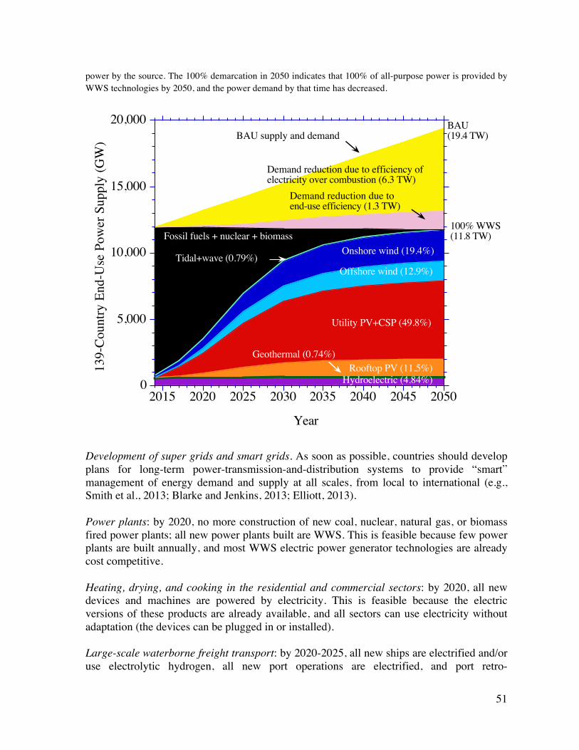
51

power by the source. The 100% demarcation in 2050 indicates that 100% of all-purpose power is provided by WWS technologies by 2050, and the power demand by that time has decreased.

Development of super grids and smart grids. As soon as possible, countries should develop plans for long-term power-transmission-and-distribution systems to provide “smart” management of energy demand and supply at all scales, from local to international (e.g., Smith et al., 2013; Blarke and Jenkins, 2013; Elliott, 2013). Power plants: by 2020, no more construction of new coal, nuclear, natural gas, or biomass fired power plants; all new power plants built are WWS. This is feasible because few power plants are built annually, and most WWS electric power generator technologies are already cost competitive. Heating, drying, and cooking in the residential and commercial sectors: by 2020, all new devices and machines are powered by electricity. This is feasible because the electric versions of these products are already available, and all sectors can use electricity without adaptation (the devices can be plugged in or installed). Large-scale waterborne freight transport: by 2020-2025, all new ships are electrified and/or use electrolytic hydrogen, all new port operations are electrified, and port retro-

0

5,000

10,000

15,000

20,000

2015 2020 2025 2030 2035 2040 2045 2050

139-

Coun

try E

nd-U

se P

ower

Sup

ply

(GW

)

Year

Hydroelectric (4.84%)

Demand reduction due to efficiency ofelectricity over combustion (6.3 TW)

Demand reduction due to end-use efficiency (1.3 TW)

Onshore wind (19.4%)Fossil fuels + nuclear + biomass

Offshore wind (12.9%)

Utility PV+CSP (49.8%)

Rooftop PV (11.5%)Geothermal (0.74%)

Tidal+wave (0.79%)

BAU supply and demand

100% WWS(11.8 TW)

BAU(19.4 TW)

52

electrification is well underway. This should be feasible for relatively large ships and ports because large ports are centralized and few ships are built each year. Policies may be needed to incentivize the early retirement of ships that do not naturally retire before 2050. Rail and bus transport: by 2025, all new trains and buses are electrified. This requires changing the supporting energy-delivery infrastructure and the manufacture method of transportation equipment. However, relatively few producers of buses and trains exist, and the supporting energy infrastructure is concentrated in cities. Off-road transport, small-scale marine: by 2025 to 2030, all new production is electrified. Heavy-duty truck transport: by 2025 to 2030, all new heavy-duty trucks and buses are electrified or use electrolytic hydrogen. It may take 10-15 years for manufacturers to retool and for enough of the supporting energy-delivery infrastructure to be put in place. Light-duty on-road transport: by 2025-2030, all new light-duty onroad vehicles are electrified. Manufacturers need time to retool, but more importantly, several years are needed to get the energy-delivery infrastructure in place for a 100% WWS transportation fleet.. Short-haul aircraft: by 2035, all new small, short-range aircraft are battery- or electrolytic-hydrogen powered. Changing the design and manufacture of airplanes and the design and operation of airports are the main limiting factors to a more rapid transition. Long-haul aircraft: by 2040, all remaining new aircraft use electrolytic cryogenic hydrogen (Jacobson and Delucchi, 2011, Section A.2.7) with electricity power for idling, taxiing, and internal power. The limiting factors to a faster transition are the time and social changes required to redesign aircraft and airports. During the transition, conventional fuels and existing WWS technologies are needed to produce the remaining WWS infrastructure. However, much of the conventional energy would be used in any case to produce conventional power plants and automobiles if the plans proposed here were not implemented. Further, as the fraction of WWS energy increases, conventional energy generation will decrease, ultimately to zero, at which point all new WWS devices will be produced with existing WWS. In sum, the creation of WWS infrastructure may result in a temporary increase in emissions before they are ultimately reduced to zero. Figure 12 illustrates the impact on global carbon dioxide levels of the aggressive goals proposed here (80% WWS by 2030 and 100% by 2050) as well as of a less aggressive scenario that provides 80% WWS by 2050 and 100% by 2100. Both scenarios reduce CO2 levels below those today. The 100% by 2050 scenario reduces CO2 to 370 ppmv by 2050, a level last seen around 2000, and to 350 ppmv by 2065. By 2100, CO2 would be reduced to 321 ppmv, a level last seen around 1966. Merely maintaining a constant emission rate, which is a conservative assumption because emissions are increasing rather than staying

53

constant today, results in CO2 increasing to 500 ppmv by 2100. All IPCC (2000) emission scenarios similarly result in CO2 levels much higher than in WWS scenarios through 2100. Further, the WWS plans proposed here will eliminate energy-related black carbon, the second-leading cause of global warming after carbon dioxide, and energy-related methane, the third-leading cause, as well as tropospheric ozone precursors, carbon monoxide, and nitrous oxide from energy. As such the aggressive worldwide conversion to WWS proposed here will avoid exploding levels of CO2 and other global warming contaminants, potentially avoiding catastrophic climate change. Figure 12. Change in world CO2 mixing ratio (ppmv) resulting from five Intergovernmental Panel on Climate Change (IPCC) scenarios (IPCC, 2000), a case assuming constant current emissions, in a 100% by 2050 WWS case from Figure 11, and in a less-aggressive 80% by 2050 and 100% by 2100 case.

The curves are derived from Equation 3.22 of Jacobson (2012). They assume a 2015 mixing ratio of CO2 of 400 ppmv, a pre-industrial CO2 mixing ratio of 275 ppmv, and a data-constrained CO2 lifetime of 50 years (Jacobson, 2012). In the WWS cases, they assume an initial fossil-fuel CO2 emission rate of 9860 Tg-C/year (Le Quere et al., 2015), reduced by 80% by 2030 and 100% by 2050 in one case and 80% by 2050 and 100% by 2100 in the other. In both cases, and in the constant-emission case, a constant landuse-change CO2 emission rate of 800 Tg-C/year (Le Quere et al., 2015) was used. The IPCC scenarios used emissions for fossil fuels and landuse change directly from IPCC (2000). 2184.82 Tg-C = 1 ppmv. 11. Recommended First Steps The policy pathways necessary to transform the 139 countries treated here to 100% WWS will differ by country, depending largely on the willingness of the government and people in each country to affect rapid change. This study does not advocate specific policy measures for any country. Instead, it provides a set of policy options that each country can consider. The list is by no means complete. Within each section, the policy options are listed roughly in order of proposed priority.

300

400

500

600

700

800

2020 2040 2060 2080 2100

80% WWS by 2030 100% by 205080% WWS by 2050 100% by 2100Constant emissionsA1BA2B1B2A1F1

300

400

500

600

700

800

CO2 (p

pmv)

Year

54

12.1. Energy Efficiency Measures

• Expand clean, renewable energy standards and energy efficiency standards.

• Incentivize conversion from natural gas water and air heaters to electric heat pumps (air and ground-source) and rooftop solar thermal hot water pre-heaters.

• Promote, though municipal financing, incentives, and rebates, energy efficiency

measures in buildings and other infrastructure. Efficiency measures include, but are not limited to, using LED lighting; evaporative cooling; ductless heating and air conditioning; energy-storing materials in walls and floors to modulate temperature changes, water-cooled heat exchanging; night ventilation cooling; combined space and water heating; improved data center design; improved air flow management; advanced lighting controls; variable refrigerant flow; improved wall, floor, ceiling, and pipe insulation; double- and triple-paned windows; and passive solar heating. Additional measures include sealing windows, doors, and fireplaces; and monitoring building energy use and performing energy audits to find energy waste.

• Revise building codes to incorporate “green building standards” based on best

practices for building design, construction, and energy use.

• Incentivize landlord investment in energy efficiency. Allow owners of multi-family buildings to take a property tax exemption for energy efficiency improvements in their buildings that provide benefits to their tenants.

• Create energy performance rating systems with minimum performance requirements

to assess energy efficiency levels and pinpoint areas of improvement.

• Create a green building tax credit program for the corporate sector. 12.2. Energy Supply Measures

• Increase Renewable Portfolio Standards (RPSs).

• Extend or create state WWS production tax credits.

• Streamline the permit approval process for large-scale WWS power generators and high-capacity transmission lines. Work with local and regional governments to manage zoning and permitting issues within existing planning efforts or pre-approve sites to reduce the cost and uncertainty of projects and expedite their physical build-out.

• Streamline the small-scale solar and wind installation permitting process. Create

common codes, fee structures, and filing procedures across a country.

55

• Lock in fossil fuel and nuclear power plants to retire under enforceable commitments. Implement taxes on emissions by current utilities to encourage their phase-out.

• Incentivize clean-energy backup emergency power systems rather than

diesel/gasoline generators at both the household and community levels.

• Incentivize home or community energy storage (through garage electric battery systems, for example) that accompanies rooftop solar to mitigate problems associated with grid power losses.

12.3. Utility Planning and Incentive Structures

• Incentivize community seasonal heat storage underground using the Drake Landing solar community as an example.

• Incentive the development of utility-scale grid electric power storage, such as in CSP, pumped hydropower, and more efficient hydropower.

• Require utilities to use demand response grid management to reduce the need for short-term energy backup on the grid.

• Incentivize the use of excess WWS electricity to produce hydrogen to help manage

the grid.

• Develop programs to use EV batteries, after the end of their useful life in vehicles, for local, short-term storage and balancing.

• Implement virtual net metering (VNM) for small-scale energy systems. 12.4. Transportation

• Promote more public transit by increasing its availability and providing compensation to commuters for not purchasing parking passes.

• Increase safe biking and walking infrastructure, such as dedicated bike lanes, sidewalks, crosswalks, timed walk signals, etc.

• Adopt legislation mandating BEVs for short- and medium distance government

transportation and using incentives and rebates to encourage the transition of commercial and personal vehicles to BEVS.

• Use incentives or mandates to stimulate the growth of fleets of electric and/or hydrogen fuel cell/electric hybrid buses starting with a few and gradually growing the fleets. Also incentivize electric and hydrogen fuel cell ferries, riverboats, and other local shipping.

56

• Adopt zero-emission standards for all new on-road and off-road vehicles, with the percentage of new production required to be zero-emission increasing to 100% by 2030 at the latest.

• Ease the permitting process for installing electric charging stations in public parking

lots, hotels, suburban metro stations, on streets, and in residential and commercial garages.

• Set up time-of-use electricity rates to encourage charging at night.

• Incentivize the electrification of freight rail and shift freight from trucks to rail.

12.5. Industrial Processes

• Provide financial incentives for industry to convert to electricity and electrolytic hydrogen for high temperature and manufacturing processes.

• Provide financial incentives to encourage industries to use WWS electric power generation for on-site electric power (private) generation.

12. Summary Roadmaps are presented for converting the energy systems for all purposes (electricity, transportation, heating/cooling, industry, and agriculture/forestry/fishing) of 139 countries into clean and sustainable ones powered by wind, water, and sunlight (WWS). For each country, the study estimates 2050 BAU power demand from current data, converts the supply for each load sector to WWS supply, and proposes a mix of WWS generators within each the country that can match projected 2050 all-sector power demand. The conversion from BAU combustion to WWS electricity for all purposes is calculated to reduce 139-country-averaged end-use load by ~39.2%, with ~82% of this due to electrification and eliminating the need for mining, transport, and refining of conventional fuels, and the rest due to end-use energy efficiency improvements. Remaining all-purpose annually-averaged end-use 2050 load over the 139 countries is proposed to be met with ~1.17 million new onshore 5-MW wind turbines (providing 19.4% of 139-country power for all purposes), 762,000 off-shore 5-MW wind turbines (12.9%), 496,900 50-MW utility-scale solar-PV power plants (42.2%), 15,400 100-MW utility-scale CSP power plants with storage (7.7%), 653 million 5-kW residential rooftop PV systems (5.6%), 35.3 million 100-kW commercial/government rooftop systems (6.0%), 840 100-MW geothermal plants (0.74%), 496,000 0.75-MW wave devices (0.72%), 32,100 1-MW tidal turbines (0.07%), and 0 new hydropower plants. The capacity factor of existing hydropower plants will increase slightly so that hydropower supplies 4.8% of all-purpose power. Another estimated 9,300 100-MW CSP plants with storage and 99,400 50-MW solar thermal collectors for heat generation and storage will be needed to help stabilize the grid. This is just one possible mix of generators.

57

The additional footprint on land for WWS devices is equivalent to about 0.29% of the 139-country land area, mostly for utility scale PV. This does not account for land gained from eliminating the current energy infrastructure. An additional on-land spacing area of about 0.65% for the 139 countries is required for onshore wind, but this area can be used for multiple purposes, such as open space, agricultural land, or grazing land. The 2013 LCOE for hydropower, onshore wind, utility-scale solar, and solar thermal for heat is already similar to or less than the LCOE for natural gas combined-cycle power plants. Rooftop PV, offshore wind, tidal, and wave presently have higher LCOEs. However, by 2050 the LCOE for all WWS technologies is expected to drop, most significantly for offshore wind, tidal, wave, rooftop PV, CSP, and utility PV, whereas conventional fuel costs are expected to rise. The 139-country roadmaps are anticipated to create 24.0 million 35-year construction jobs and 26.5 million 35-year operation jobs for the energy facilities alone, the combination of which would outweigh by ~22.1 million the 28.4 million jobs lost in the conventional energy sector. The 139-country roadmaps will eliminate ~4.6 (1.3-8.0) million premature air pollution mortalities per year today and 3.3 (0.8-7.0) million/yr in 2050, avoiding ~$25.4 ($4.3-$69.7) trillion/year in 2050 air-pollution damage costs (2013 dollars), equivalent to ~7.9 (1.3-21.6) percent of the 2050 139-country GDP. Converting will further eliminate ~$17 (9.6-36) trillion/year in 2050 global warming costs (2013 dollars) due to 139-country greenhouse-gas and particle emissions. These plans will result in the average person in 2050 saving $170/year in fuel costs compared with conventional fuels, ~2,880/person/year in air-pollution-damage cost and ~$1,930/person/year in climate costs (2013 dollars). Many uncertainties in the analysis here are captured in broad ranges of energy, health, and climate costs given. However, these ranges may miss costs due to limits on supplies caused by wars or political/social opposition to the roadmaps. As such, the estimates should be reviewed periodically. The timeline for conversion is proposed as follows: 80% of all energy to be WWS by 2030 and 100% by 2050. As of the end of 2014, three countries -- Norway (67%), Paraguay (54%), and Iceland (39%) – have installed more than 35% of their projected all-purpose 2050 needed nameplate capacity of WWS energy. The world average conversion to date is 3.8%. The major benefits of a conversion are the near-elimination of air pollution morbidity and mortality and global warming, net job creation, energy-price stability, reduced international conflict over energy because each country will largely be energy independent, increased accessed to distributed energy and reduced energy poverty to the 4 billion people worldwide who currently collect their own energy and burn it, and reduced risks of large-scale system

58

disruptions because much of the world power supply will be decentralized. Finally, the aggressive worldwide conversion to WWS proposed here will avoid exploding levels of CO2 and catastrophic climate change. The study finds that the conversion to WWS is technically and economically feasible. The main barriers are still social and political. Acknowledgments We would like to thank The Solutions Project for partial funding of three students. The spreadsheets for this paper can be found in Delucchi et al. (2015). References Anenberg, S.C., D. Shindell, M. Amann, G. Faluvegi, et al., 2012. Global air quality and health co-benefits of

mitigating near-term climate change through methane and black carbon emission controls, Environmental Health Perspectives, 120, 831-839.

Arent, D., P. Sullivan, D. Heimiller, A. Lopez, K. Eurek, J. Badger, H.E. Jorgensen, and M. Kelly, 2015, 2012, Improved offshore wind resource assessment in global climate stabilization scenarios, NREL/TP-6A20-55049, http://www.nrel.gov/docs/fy13osti/55049.pdf, Accessed June 11, 2015.

Bertani, R., 2015. Geothermal Power Generation in the World 2010-2014 Update Report, World Geothermal Congress 2015 Conference Proceedings, Melbourne, Australia, 19-25 April 2015.

Beyond Zero Emissions, Zero Carbon Australia Stationary Energy Plan, Melbourne Energy Institute, University of Melbourne, July, 2010. http://media.bze.org.au/ZCA2020_Stationary_Energy_Report_v1.pdf, Accessed May 2, 2015.

Blarke, M. B., and B. M. Jenkins, 2013. SuperGrid or SmartGrid: Competing Strategies for large-scale integration of intermittent renewables?, Energy Policy 58: 381-390.

Buonocore, J.J., P. Luckow, G. Norris, J.D. Spengler, B. Biewald, J. Fisher, and J.I. Levy, Health and climate benefits of different energy efficiency and renewable energy choices, Nat. Clim. Change, doe:10.1039/NCLIMATE2771, 2015.

Clean Line Energy Partners, 2015, Projects, http://www.cleanlineenergy.com/projects, Accessed Sept. 20, 2015.

Connolly, D., and B.V. Mathiesen, 2014, A technical and economic analysis of one potential pathway to a 100% renewable energy system, Intl. J. Sustainable Energy Planning & Management, 1, 7-28.

CSP World, 2015. CSP world map. http://www.cspworld.org/cspworldmap. Accessed July 22, 2015. Delucchi, M.A., Jacobson, M.Z., 2011. Providing all global energy with wind, water, and solar power, Part II:

Reliability, System and Transmission Costs, and Policies. Energy Policy, 39, 1170-1190, doi:10.1016/j.enpol.2010.11.045.

Delucchi, M.A., M.Z. Jacobson, Z.A.F. Bauer, S. Goodman, and W. Chapman, 2015. Spreadsheets for 139-country 100% wind, water, and solar roadmaps, http://web.stanford.edu/group/efmh/jacobson/Articles/I/WWS-50-USState-plans.html. Accessed November 18, 2015.

DOE (Department of Energy, U.S.), 2012. An Assessment of Energy Potential at Non-Powered Dams in the United states, http://nhaap.ornl.gov/system/files/NHAAP_NPD_FY11_Final_Report.pdf. Accessed December 17, 2012.

Dulac, J., 2013. Global Land Transport Infrastructure Requirements, International Energy Agency, https://www.iea.org/publications/freepublications/publication/TransportInfrastructureInsights_FINAL_WEB.pdf, Accessed September 9, 2015.

Dvorak, M., C.L. Archer, and M.Z. Jacobson, 2010. California offshore wind energy potential, Renewable Energy, 35, 1244-1254, doi:10.1016/j.renene.2009.11.022.

ECF (European Climate Foundation), 2010, Roadmap 2050: A Practical Guide to a Prosperous, Low-Carbon Europe, http://www.roadmap2050.eu/project/roadmap-2050, Accessed May 2, 2015.

EIA (Energy Information Agency), 2015. International Energy Outlook, 2014, http://www.eia.gov/forecasts/ieo/, Accessed November 17, 2015.

Eiffert, P., 2003. Non-technical barriers to the commercialization of PV power systems in the built environment, NREL/TP-550-31976, http://www.nrel.gov/docs/fy03osti/31976.pdf, Accessed September 8, 2015.

59

Elliott, D., 2013. Emergence of European supergrids – Essay on strategy issues, Energy Strategy Reviews 1: 171-173.

ELTE/EENA (ELTE University sustainable energy research group/Environmental education network association), 2014, Hungarian sustainable energy vision, http://inforse.dk/europe/VisionHU.htm, Accessed May 2, 2015.

Entranze Data Tool, 2015. .Intelligent Energy Europe Program, European Union. http://www.entranze.enerdata.eu/, Accessed September 8, 2015.

EPIA (European Photovoltaic Industry Association) 2014. Global Market Outlook for Photovoltaics 2014-2020, http://www.epia.org/fileadmin/user_upload/Publications/44_epia_gmo_report_ver_17_mr.pdf, Accessed 27 July 2015.

EREC (European Renewable Energy Council), 2010, RE-Thinking 2050: A 100% Renewable Energy Vision for the European Union, http://www.erec.org/fileadmin/erec_docs/Documents/Publications/ReThinking2050_full%20version_final.pdf, Accessed May 2, 2015.

GCP (Global Carbon Project), Global Carbon Budget 2014 spreadsheet, Territorial Emissions, http://www.globalcarbonproject.org/carbonbudget/14/data.htm, Accessed August 12, 2015.

GWEC (Global Wind Energy Council), 2015. Global wind report annual market update 2014, http://www.gwec.net/wp-content/uploads/2015/03/GWEC_Global_Wind_2014_Report_LR.pdf, Accessed July 15, 2015.

Hooker-Stroud, A., P. James, T. Kellner, and P Allen, 2015. Understanding the challenges and opportunities in managing hourly variability in a 100% renewable energy system for the UK, Carbon Management, doi:10.1080/17583004.2015.1024955.

IEA (International Energy Agency), 2014a. 2014 Key world energy statistics, http://www.iea.org/publications/freepublications/publication/keyworld2014.pdf, Accessed August 1, 2015.

IEA (International Energy Agency), 2014b, Renewable energy medium-term market report 2014. IEA (International Energy Agency), 2015, Statistics, http://www.iea.org/statistics/statisticssearch/, Accessed

June 10, 2015. IEA-PVPS (International Energy Agency-Photovoltaic Power Systems Programme) 2015, PVPS Annual

report 2014, http://iea-pvps.org/index.php?id=6&eID=dam_frontend_push&docID=2557, Accessed 25 July 2015.

IEA (International Energy Agency), 2005, Energy use in the new millennium, https://www.iea.org/publications/freepublications/publication/millennium.pdf, Accessed Sept. 8, 2015.

IHA (International Hydropower Association), 2015, Country profiles, http://www.hydropower.org/country-profiles, Accessed August 1, 2015.

IPCC (Intergovernmental Panel on Climate Change), 2000. Special Report on Emission Scenarios (SRES), http://sres.ciesin.org/final_data.html, Accessed November 19, 2015.

Jacobson, M.Z., W.G. Colella, and D.M. Golden, 2005. Cleaning the air and improving health with hydrogen fuel cell vehicles, Science, 308, 1901-1905.

Jacobson, M.Z., Y.J. Kaufmann, Y. Rudich, 2007, Examining feedbacks of aerosols to urban climate with a model that treats 3-D clouds with aerosol inclusions, J. Geophys. Res., 112, D24205, doi:10.1029/2007JD008922.

Jacobson, M.Z., 2009. Review of solutions to global warming, air pollution, and energy security, Energy & Environmental Science, 2, 148-173, doi:10.1039/b809990c.

Jacobson, M.Z., and M.A. Delucchi, November 2009. A path to sustainable energy by 2030, Scientific American.

Jacobson, M.Z., 2010. Enhancement of local air pollution by urban CO2 domes, Environmental Science, and Technology, 44, 2497-2502.

Jacobson, M.Z., 2010, Short-term effects of controlling fossil-fuel soot, biofuel soot and gases, and methane on climate, Arctic ice, and air pollution health, J. Geophys. Res., 115, D14209, doi:10.1029/2009JD013795.

Jacobson, M.Z., and M.A. Delucchi, 2011. Providing all Global Energy with Wind, Water, and Solar Power, Part I: Technologies, Energy Resources, Quantities and Areas of Infrastructure, and Materials, Energy Policy, 39, 1154-1169, doi:10.1016/j.enpol.2010.11.040.

Jacobson, M. Z., 2012. Air Pollution and Global Warming: History, Science, and Solutions, Second Edition, Cambridge University Press, Cambridge, 375 pp.

Jacobson, M.Z., R.W. Howarth, M.A. Delucchi, S.R. Scobies, J.M. Barth, M.J. Dvorak, M. Klevze, H. Katkhuda, B. Miranda, N.A. Chowdhury, R. Jones, L. Plano, and A.R. Ingraffea, 2013. Examining the feasibility of converting New York Country’s all-purpose energy infrastructure to one using wind, water, and sunlight, Energy Policy, 57, 585-601.

Jacobson, M.Z., M.A. Delucchi, A.R. Ingraffea, R.W. Howarth, G. Bazouin, B. Bridgeland, K. Burkhart, M. Chang, N. Chowdhury, R. Cook, G. Escher, M. Galka, L. Han, C. Heavey, A. Hernandez, D.F. Jacobson, D.S. Jacobson, B. Miranda, G. Novotny, M. Pellat, P. Quach, A. Romano, D. Stewart, L. Vogel, S. Wang,

60

H. Wang, L. Willman, T. Yeskoo, 2014. A roadmap for repowering California for all purposes with wind, water, and sunlight, Energy, 73, 875-889, doi:10.1016/j.energy.2014.06.099.

Jacobson, M.Z., M.A. Delucchi, G. Bazouin, Z.A.F. Bauer, C.C. Heavey, E. Fisher, S. B. Morris, D.J.Y. Piekutowski, T.A. Vencill, T.W. Yeskoo, 2015a, 100% clean and renewable wind, water, sunlight (WWS) all-sector energy roadmaps for the 50 United States, Energy and Environmental Sciences, 8, 2093-2117, doi:10.1039/C5EE01283J.

Jacobson, M.Z., M.A. Delucchi, M.A. Cameron, and B.A. Frew, 2015b. A low-cost solution to the grid reliability problem with 100% penetration of intermittent wind, water, and solar for all purposes, Proc. Nat. Acad. Sci., 112, doi: 10.1073/pnas.1510028112.

Jacobson, M.Z., M.A. Delucchi, G. Bazouin, M.J. Dvorak, R. Arghandeh, Z. A.F. Bauer, A. Cotte, G.M.T.H. de Moor, E.G. Goldner, C. Heier, R.T. Holmes, S.A. Hughes, L. Jin, M. Kapadia, C. Menon, S.A. Mullendore, E.M. Paris, G.A. Provost, A.R. Romano, C. Srivastava, T.A. Vencill, N.S. Whitney, and T.W. Yeskoo, 2016a, A 100% wind, water, sunlight (WWS) all-sector energy plan for Washington State, Renewable Energy, 86, 75-88.

Jacobson, M.Z., C. Clack, M.A. Delucchi, M.C. Cameron, 2016b, 100% grid reliability in 20 regions of the world with 100% penetration of intermittent wind, water, and solar for all purposes, in preparation.

JPL (Jet Propulsion Laboratory), 2010, Dataset Discovery, http://podaac.jpl.nasa.gov/datasetlist?ids=Platform&values=QUIKSCAT, Processed by D. Whitt and M. Dvorak, Accessed February 23, 2012.

Lepeule, J., F. Laden, D. Dockery, and J. Schwartz, 2012. Chronic exposure to fine particles and mortality: An extended follow-up of the Harvard six cities study from 1974 to 2009, Environmental Health Perspectives, 120, 965-970.

LeQuere et al., 2015, Global carbon budget 2014, Earth Syst. Sci. Data 7, 47-85, 2015.  Linowes, L., 2012. Wind Benefit Inflation: JEDI (NREL) Model Needs Reality Check.

http://www.masterresource.org/2012/12/wind-benefit-inflation-jedi-nrel-2/, Accessed Dec. 16, 2012. Lund, J. W. and T.L. Boyd, 2015. Direct Utilization of Geothermal Energy 2015 Worldwide Review, World

Geothermal Congress 2015 Conference Proceedings, Melbourne, Australia, 19-25 April 2015. Marine Renewables Canada, 2013. Marine renewable energy in Canada and the global context,

http://www.marinerenewables.ca/wp-content/uploads/2012/11/State-of-the-Canadian-MRE-Sector-20131.pdf, Accessed August 1, 2015.

Mathiesen, B.V., H. Lund, D. Connolly, H. Wenzel, P.A. Ostergaard, B. Moller, S. Nielsen, I. Ridjan, P. Kamoe, K. Sperling, F.K. Hvelplund, 2015, Smart energy systems for coherent 100% renewable energy and transport solutions, Applied Energy, 145, 139-154.

Negawatt Association, 2015. The Negawatt 2050 scenario, http://www.negawatt.org/english-presentation-p149.html, Accessed July 31, 2015.

NREL (National Renewable Energy Laboratory), 2012a. Wind resources by class and country at 50 m, http://en.openei.org/datasets/dataset/wind-resources-by-class-and-country-at-50m, Accessed June 11, 2015.

NREL (National Renewable Energy Laboratory), 2012b. Global Solar Opportunity Tool, http://maps.nrel.gov/global_re_opportunity#, Accessed September 9, 2015.

NREL (National Renewable Energy Laboratory), 2013, Jobs and Economic Development Impact Models (JEDI). http://www.nrel.gov/analysis/jedi/download.html. Accessed October 27, 2013.

NREL (National Renewable Energy Laboratory), 2015, Concentrating Solar Power Projects by Country. http://www.nrel.gov/csp/solarpaces/by_country.cfm. Accessed July 22, 2015.

OECD (2014), The Cost of Air Pollution: Health Impacts of Road Transport, OECD Publishing, Paris. DOI: http://dx.doi.org/10.1787/9789264210448-en.

Parsons-Brinckerhoff, Powering the Future: Mapping our Low-Carbon Path to 2050, Dec. (2009). https://www.pbworld.com/pdfs/powering_the_future/pb_ptf_full_report.pdf, Accessed May 2, 2015.

Pope, C.A. III, R.T. Burnett, M.J. Thun, E.E. Calle, D. Krewski, K. Ito, and G.D. Thurston, 2002. Lung cancer, cardiopulmonary mortality, and long-term exposure to fine particulate air pollution, Journal Amer. Med. Assoc., 287, 1132-1141.

Price-Waterhouse-Coopers, 100% Renewable Electricity: A roadmap to 2050 for Europe and North Africa, 2010, www.pwcwebcast.co.uk/dpliv_mu/100_percent_renewable_electricity.pdf, Accessed May 2, 2015.

REN21 (Renewable Energy Policy Network for the 21st Century), 2015, Renewables 2015 Global Status Report, http://www.ren21.net/wp-content/uploads/2015/07/REN12-GSR2015_Onlinebook_low_nolinks.pdf, Accessed 1 August 2015.

Shindell, D., J.C.I. Kuylenstierna, E. Vignati, R. van Dingenen, M. Amann et al., 2012. Simultaneously mitigating near-term climate change and improving human health and food security, Science, 335, 183-189.

61

Smith, J. C., et al., 2013. Transmission planning for wind energy in the United States and Europe: status and prospects, WIREs Energy Environ 2: 1-13.

Teske, S., S. Sawyer, O. Schafer, T. Pregger, S. Simon, and T. Naegler, 2015, Energy revolution: A sustainable world energy outlook 2015, http://www.greenpeace.org/international/en/publications/Campaign-reports/Climate-Reports/Energy-Revolution-2015/, Accessed Sept. 22, 2015.

WHO (World Health Organization), 2014. 7 million premature deaths annually linked to air pollution, http://www.who.int/mediacentre/news/releases/2014/air-pollution/en/, Accessed June 15, 2015.

WHO, 2014, Global Health Observatory Data Repository, http://apps.who.int/gho/data/node.main.156 Accessed 2 July 2015.

World Bank, 2015a, World development indicators: Contribution of natural resources to gross domestic product, http://wdi.worldbank.org/table/3.15#, Accessed June 17, 2015.

World Bank, 2015b, Labor force, total, http://data.worldbank.org/indicator/SL.TLF.TOTL.IN/countries, Accessed June 17, 2015.

World Bank, 2015c, Urban population (% of total), http://data.worldbank.org/indicator/SP.URB.TOTL.IN.ZS, Accessed September 8, 2015.

World Bank, 2014, Infrastructure, Passenger cars (Per 1000 people), http://data.worldbank.org/indicator/IS.VEH.PCAR.P3, Accessed Fall 2014

World Bank, 2015, Electricity production from hydroelectric sources, http://data.worldbank.org/indicator/EG.ELC.HYRO.ZS, Accessed August 1, 2015.

Zero Carbon Britain, 2013, Zero Carbon Britain: Rethinking the future, http://zerocarbonbritain.org/images/pdfs/ZCBrtflo-res.pdf, Accessed May 2, 2015.

Exhibit 30

100% OREGONTransition to 100% wind, water, and solar (WWS) for all purposes

(electricity, transportation, heating/cooling, industry)

Residential rooftop PV4%

Solar PV plants8%

CSP plants5%

Onshore wind32.5%

Offshore wind15%

Commercial/govtrooftop PV

2.2%

Wave devices1%

Geothermal5%

Hydroelectric27.3%

Tidal turbines0.05%

2050PROJECTED

ENERGY MIX

40-Year Jobs CreatedNumber of jobs where a personis employed for 40 consecutive years

Operation jobs:

Construction jobs:

=10,000

14,235

21,564

Using WWS electricity for everything, instead of burning fuel, andimproving energy efficiency means you need much less energy.

-40.4%

Current demand Wind, Water, Solar

VISIT THESOLUTIONSPROJECT.ORGTO LEARN MORE AND 100.ORG TO JOIN THE MOVEMENT

Data from Stanford University - For more information, visithttp://go100.me/50StateTargets

FO L LOW U S O N 100isNow SolutionsProj

100% OREGON

VISIT THESOLUTIONSPROJECT.ORGTO LEARN MORE AND 100.ORG TO JOIN THE MOVEMENT

Data from Stanford University - For more information, visithttp://go100.me/50StateTargets

FO L LOW U S O N 100isNow SolutionsProj

P

Transition to 100% wind, water, and solar (WWS) for all purposes(electricity, transportation, heating/cooling, industry)

Avoided Mortality and Illness Costs Percentage of Oregon Land Needed forAll New WWS Generators

Future Energy Costs 2050 Money in Your Pocket

Avoided health costs per year:

1.3% of State GDP

Air pollution deaths avoided every year: 453

$5.3B

=100

Plan pays for itself in as little as 3.1 years from air pollution and climatecost savings alone

0.63%Spacing area

0.06%Footprint area

BAU (Business as usual) WWS (Wind, water, solar)

U.S. average fossil-fuel energy costs*

9.02 c/kWh

State average WWS electricity costs

10.01 c/kWh

*Health and climate external costs of fossil fuels are another 5.7c/kWh

Annual energy, health, and climate cost savings per personin 2050: $5,232

Annual energy cost savings per person in 2050: $33

= $2,000

Exhibit 31

Careful what you wish for 1

Be careful of what you wish for

The economic impacts of Queensland’s unconventional gas experiment and the

implications for Northern Territory policy makers.

Discussion paper

Mark Ogge November 2015

2 The economic impacts of Queensland’s unconventional gas experiment and the implications for Northern Territory policy makers.

ABOUT THE AUSTRALIA INSTITUTE

The Australia Institute is an independent public policy think tank based in Canberra. It

is funded by donations from philanthropic trusts and individuals and commissioned

research. Since its launch in 1994, the Institute has carried out highly influential

research on a broad range of economic, social and environmental issues.

OUR PHILOSOPHY

As we begin the 21st century, new dilemmas confront our society and our planet.

Unprecedented levels of consumption co-exist with extreme poverty. Through new

technology we are more connected than we have ever been, yet civic engagement is

declining. Environmental neglect continues despite heightened ecological awareness.

A better balance is urgently needed.

The Australia Institute’s directors, staff and supporters represent a broad range of

views and priorities. What unites us is a belief that through a combination of research

and creativity we can promote new solutions and ways of thinking.

OUR PURPOSE – ‘RESEARCH THAT MATTERS’

The Institute aims to foster informed debate about our culture, our economy and our

environment and bring greater accountability to the democratic process. Our goal is to

gather, interpret and communicate evidence in order to both diagnose the problems

we face and propose new solutions to tackle them.

The Institute is wholly independent and not affiliated with any other organisation. As

an Approved Research Institute, donations to its Research Fund are tax deductible for

the donor. Anyone wishing to donate can do so via the website at

https://www.tai.org.au or by calling the Institute on 02 6130 0530. Our secure and

user-friendly website allows donors to make either one-off or regular monthly

donations and we encourage everyone who can to donate in this way as it assists our

research in the most significant manner.

Level 5, 131 City Walk

Canberra, ACT 2601

Tel: (02) 61300530

Email: mail@tai.org.au

Website: www.tai.org.au

Careful what you wish for 3

Summary

The gas industry says that unconventional gas development brought an economic and

jobs boom to Queensland, and promises the same for the Northern Territory.

Territorians should test the claims of the industry in Queensland to determine the

likely economic and jobs impacts of unconventional gas development in the Northern

Territory.

In contrast to the economic benefits promised , recent gas industry funded studies of

the economic and social impacts of gas in Queensland’s unconventional gas fields have

found:

Local business stakeholders reported a deterioration in: o Financial capital o Local Infrastructure o Local skills o Social cohesion o The local environment

Unconventional gas has reduced community wellbeing: o Fewer than one in four local people approved of the unconventional gas

industry, with less than 6% believing it would “lead to something better”.

Unconventional gas creates few additional jobs: o There were virtually no spillover jobs created in local retail or

manufacturing. o Gas jobs will be slashed by 80% at the end of the construction period.

For every 10 unconventional gas jobs created, 7 service sector jobs were lost.

Figure 1: The impact of unconventional gas development on local businesses.

How did local business stakeholders in Queensland’s Darling Downs perceive the impact of unconventional gas and mining on their region? Source: CSRM University of Queensland

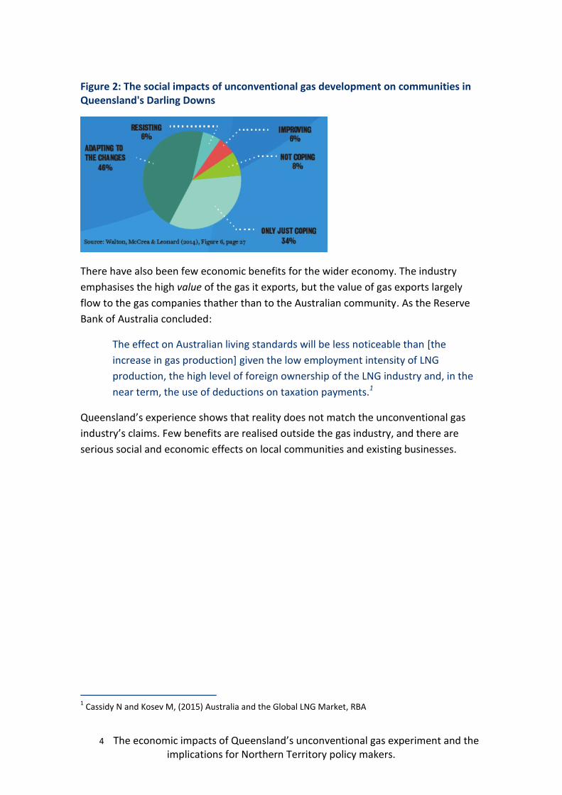
4 The economic impacts of Queensland’s unconventional gas experiment and the implications for Northern Territory policy makers.

Figure 2: The social impacts of unconventional gas development on communities in Queensland's Darling Downs

There have also been few economic benefits for the wider economy. The industry

emphasises the high value of the gas it exports, but the value of gas exports largely

flow to the gas companies thather than to the Australian community. As the Reserve

Bank of Australia concluded:

The effect on Australian living standards will be less noticeable than [the

increase in gas production] given the low employment intensity of LNG

production, the high level of foreign ownership of the LNG industry and, in the

near term, the use of deductions on taxation payments.1

Queensland’s experience shows that reality does not match the unconventional gas

industry’s claims. Few benefits are realised outside the gas industry, and there are

serious social and economic effects on local communities and existing businesses.

1 Cassidy N and Kosev M, (2015) Australia and the Global LNG Market, RBA

Careful what you wish for 5

Table of Contents

Summary ........................................................................................................................... 3

Table of Contents ............................................................................................................. 5

Introduction ...................................................................................................................... 6

1. The impacts of unconventional gas developments on local businesses ...................... 8

2. Impacts on local communities .................................................................................... 12

3. Unconventional gas does not employ many people. ................................................. 14

4. Promise versus reality ................................................................................................ 16

5. Boom and bust ............................................................................................................ 19

6. Impacts on manufacturing.......................................................................................... 21

7. Big numbers, small benefits ....................................................................................... 24

4. The Industrial footprint of shale gas .......................................................................... 25

Conclusion ...................................................................................................................... 26

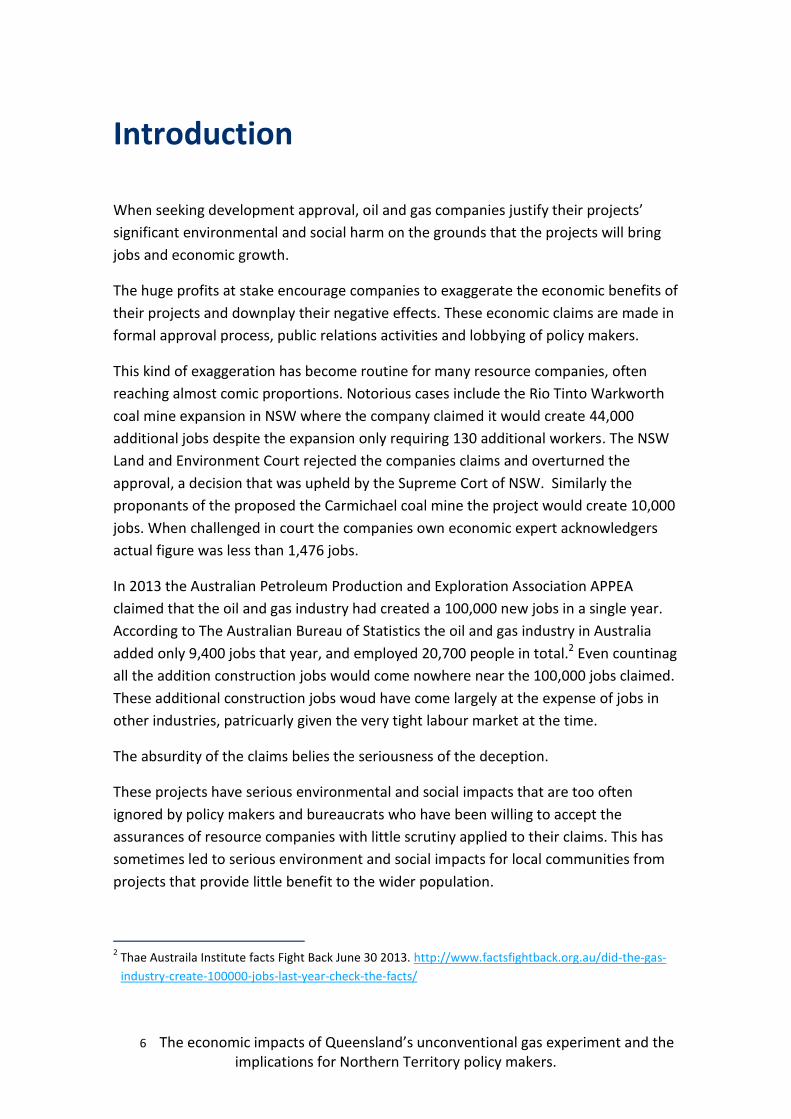
6 The economic impacts of Queensland’s unconventional gas experiment and the implications for Northern Territory policy makers.

Introduction

When seeking development approval, oil and gas companies justify their projects’

significant environmental and social harm on the grounds that the projects will bring

jobs and economic growth.

The huge profits at stake encourage companies to exaggerate the economic benefits of

their projects and downplay their negative effects. These economic claims are made in

formal approval process, public relations activities and lobbying of policy makers.

This kind of exaggeration has become routine for many resource companies, often

reaching almost comic proportions. Notorious cases include the Rio Tinto Warkworth

coal mine expansion in NSW where the company claimed it would create 44,000

additional jobs despite the expansion only requiring 130 additional workers. The NSW

Land and Environment Court rejected the companies claims and overturned the

approval, a decision that was upheld by the Supreme Cort of NSW. Similarly the

proponants of the proposed the Carmichael coal mine the project would create 10,000

jobs. When challenged in court the companies own economic expert acknowledgers

actual figure was less than 1,476 jobs.

In 2013 the Australian Petroleum Production and Exploration Association APPEA

claimed that the oil and gas industry had created a 100,000 new jobs in a single year.

According to The Australian Bureau of Statistics the oil and gas industry in Australia

added only 9,400 jobs that year, and employed 20,700 people in total.2 Even countinag

all the addition construction jobs would come nowhere near the 100,000 jobs claimed.

These additional construction jobs woud have come largely at the expense of jobs in

other industries, patricuarly given the very tight labour market at the time.

The absurdity of the claims belies the seriousness of the deception.

These projects have serious environmental and social impacts that are too often

ignored by policy makers and bureaucrats who have been willing to accept the

assurances of resource companies with little scrutiny applied to their claims. This has

sometimes led to serious environment and social impacts for local communities from

projects that provide little benefit to the wider population.

2 Thae Austraila Institute facts Fight Back June 30 2013. http://www.factsfightback.org.au/did-the-gas-

industry-create-100000-jobs-last-year-check-the-facts/

Careful what you wish for 7

The huge unconventional gas projects approved in Queensland in 2010 are a case in

point. The economic claims of the proponants were not tested by the government,

despite its obligation to objectively assess the projects. Recent research examined in

this paper clearly shows that few of the promised benefits have materialised and

existing businesses and entire industries have been badly affected. Long-term jobs

have been sacrificed for short-term gas construction jobs.

Only 6% of local people living in gasfield areas think that the industry has improved

their lives – as many as are actively resisting it. As well as active resisters, a further 42%

say that they are “not coping” or “only just coping” with the changes the industry has

made to their lives. Actual royalty payments are a small fraction of the estimates made

at approval and flow on economic activity failed to materialse, as companies bypassed

local industry and suppliers in favour of global supply chains.

The Northern Territory government has issued unconventional gas licenses for almost

the entire territory. Speculative gas interests have a strong incentive to increase the

value of their licenses by gaining environmental approvals and government promises

to subsidise infrastructure.

Northern Territory policy makers can learn from the experience in Queensland. The

economic claims of the unconventional gas industry must be subject to scrutiny and

due diligence. Projects should only proceed if they provide a net benefit to the

Territory community, not just quick profits for gas companies.

8 The economic impacts of Queensland’s unconventional gas experiment and the implications for Northern Territory policy makers.

1. The impacts of unconventional gas

developments on local businesses

While some people and businesses benefit from unconventional gas development,

many other businesses and industries can be negatively impacted and jobs in other

sectors are often lost as a result.

The most advanced unconventional gas development in Australia is in Queensland’s

Darling Downs. The gas industry uses this region as an example of the economic

benefits that unconventional gas provides local communities. The research tells a more

complicated story.

The most detailed examination of the economic impacts of unconventional gas

development in the Darling Downs is a study carried out between 2008 and 2013 by

the industry-funded Sustainable Minerals Institute SMI at the University of

Queensland. 3

This study surveyed stakeholders from different sectors in the local community

including the local business community, agriculture, local government, advocacy

groups and environmental consultants, as well as the mining and unconventional gas

industries.

The survey asked stakeholders to assess the effect of unconventional gas and mining in

the region over a five-year period on the following key indicators:

1. Financial capital: Available revenue streams and economic resources. 2. Built capital: The physical infrastructure such as buildings, transport,

equipment. 3. Social capital: The degree to which people know each other and collaborate

and the level of trust people have in local organisations and institutions. 4. Human capital: Assets such as skills, knowledge, abilities and good health

possessed by individuals that enable them to work, earn a living, contribute to society and thereby build other forms of capital.

5. Natural capital: Key natural resources, such as water, land, clean air, wildlife and forests that people can access for lifestyle or livelihood purposes.

3 Everingham, J., Collins, N., Rodriguez, D. Cavaye, J., Vink, S., Rifkin, W. & Baumgartl, T. (2013) Energy

resources from the food bowl: an uneasy co-existence. Identifying and managing cumulative impacts of

mining and agriculture. Project report. CSRM, The University of Queensland: Brisbane.

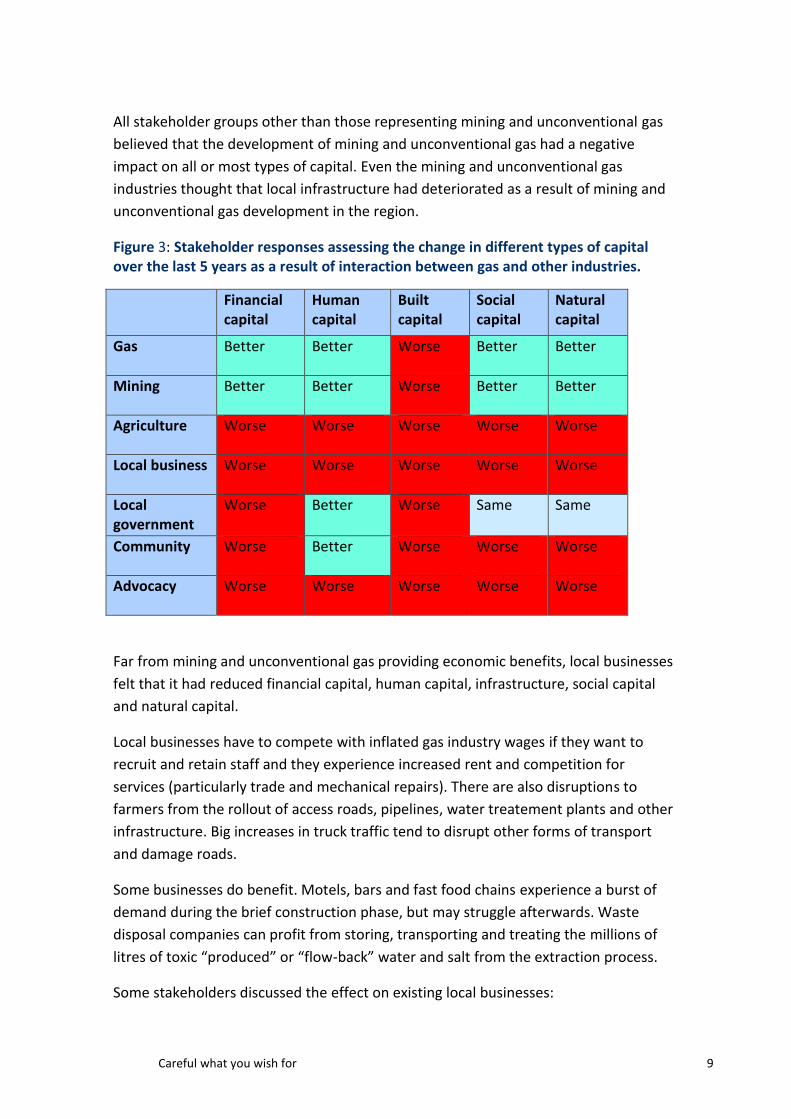
Careful what you wish for 9

All stakeholder groups other than those representing mining and unconventional gas

believed that the development of mining and unconventional gas had a negative

impact on all or most types of capital. Even the mining and unconventional gas

industries thought that local infrastructure had deteriorated as a result of mining and

unconventional gas development in the region.

Figure 3: Stakeholder responses assessing the change in different types of capital over the last 5 years as a result of interaction between gas and other industries.

Financial capital

Human capital

Built capital

Social capital

Natural capital

Gas

Better Better Worse Better Better

Mining

Better Better Worse Better Better

Agriculture

Worse Worse Worse Worse Worse

Local business

Worse Worse Worse Worse Worse

Local government

Worse Better Worse Same Same

Community

Worse Better Worse Worse Worse

Advocacy

Worse Worse Worse Worse Worse

Far from mining and unconventional gas providing economic benefits, local businesses

felt that it had reduced financial capital, human capital, infrastructure, social capital

and natural capital.

Local businesses have to compete with inflated gas industry wages if they want to

recruit and retain staff and they experience increased rent and competition for

services (particularly trade and mechanical repairs). There are also disruptions to

farmers from the rollout of access roads, pipelines, water treatement plants and other

infrastructure. Big increases in truck traffic tend to disrupt other forms of transport

and damage roads.

Some businesses do benefit. Motels, bars and fast food chains experience a burst of

demand during the brief construction phase, but may struggle afterwards. Waste

disposal companies can profit from storing, transporting and treating the millions of

litres of toxic “produced” or “flow-back” water and salt from the extraction process.

Some stakeholders discussed the effect on existing local businesses:

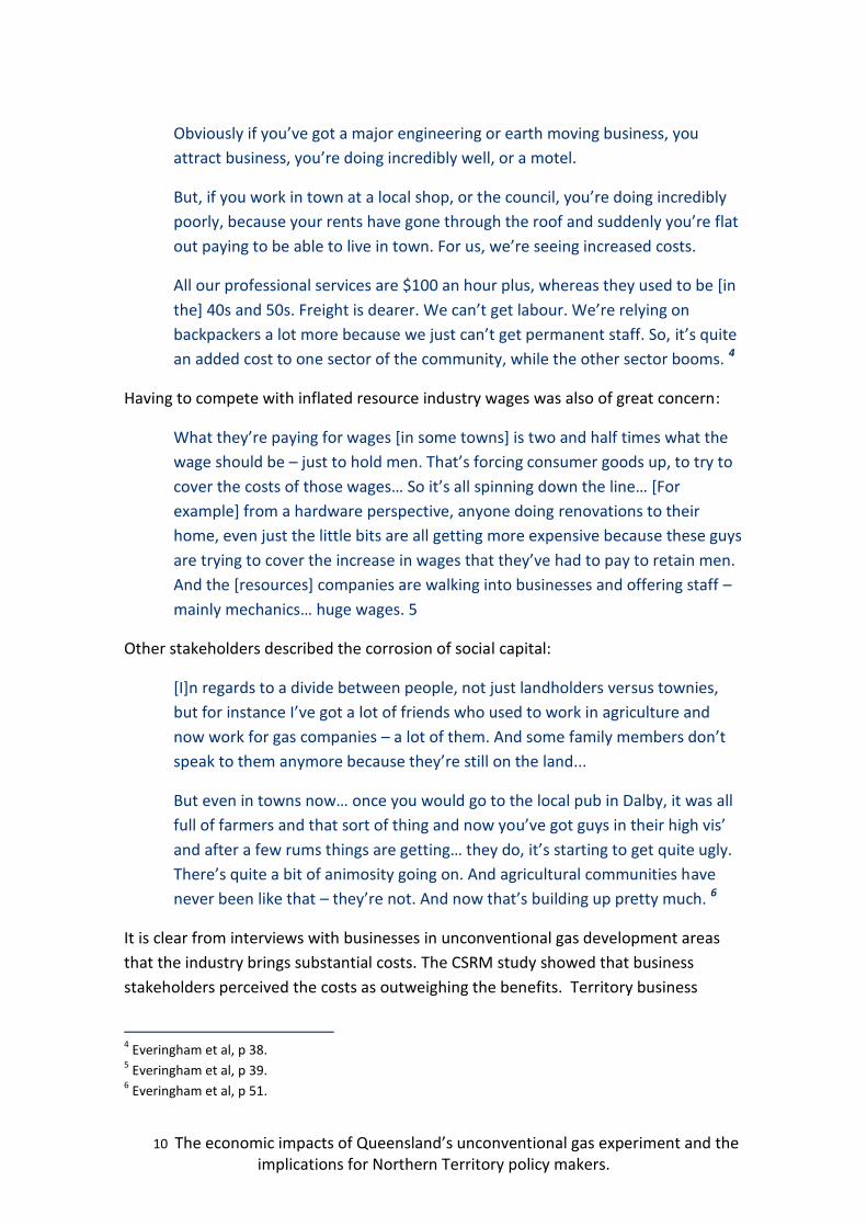
10 The economic impacts of Queensland’s unconventional gas experiment and the implications for Northern Territory policy makers.

Obviously if you’ve got a major engineering or earth moving business, you

attract business, you’re doing incredibly well, or a motel.

But, if you work in town at a local shop, or the council, you’re doing incredibly

poorly, because your rents have gone through the roof and suddenly you’re flat

out paying to be able to live in town. For us, we’re seeing increased costs.

All our professional services are $100 an hour plus, whereas they used to be [in

the] 40s and 50s. Freight is dearer. We can’t get labour. We’re relying on

backpackers a lot more because we just can’t get permanent staff. So, it’s quite

an added cost to one sector of the community, while the other sector booms. 4

Having to compete with inflated resource industry wages was also of great concern:

What they’re paying for wages [in some towns] is two and half times what the

wage should be – just to hold men. That’s forcing consumer goods up, to try to

cover the costs of those wages… So it’s all spinning down the line… [For

example] from a hardware perspective, anyone doing renovations to their

home, even just the little bits are all getting more expensive because these guys

are trying to cover the increase in wages that they’ve had to pay to retain men.

And the [resources] companies are walking into businesses and offering staff –

mainly mechanics… huge wages. 5

Other stakeholders described the corrosion of social capital:

[I]n regards to a divide between people, not just landholders versus townies,

but for instance I’ve got a lot of friends who used to work in agriculture and

now work for gas companies – a lot of them. And some family members don’t

speak to them anymore because they’re still on the land...

But even in towns now… once you would go to the local pub in Dalby, it was all

full of farmers and that sort of thing and now you’ve got guys in their high vis’

and after a few rums things are getting… they do, it’s starting to get quite ugly.

There’s quite a bit of animosity going on. And agricultural communities have

never been like that – they’re not. And now that’s building up pretty much. 6

It is clear from interviews with businesses in unconventional gas development areas

that the industry brings substantial costs. The CSRM study showed that business

stakeholders perceived the costs as outweighing the benefits. Territory business

4 Everingham et al, p 38.

5 Everingham et al, p 39.

6 Everingham et al, p 51.

Careful what you wish for 11

organisations and policy makers should be aware of how this has played out in

Queensland when considering the expansion of the gas industry in the NT.

Negative impacts on local businesses also affect communities at the social level. The

next section examines the social impacts in more detail.

12 The economic impacts of Queensland’s unconventional gas experiment and the implications for Northern Territory policy makers.

2. Impacts on local communities

Unconventional gas development in Queensland’s Darling Downs distresses local

communities. Few people approve of the industry and even fewer believe it will

improve conditions.

A recent CSIRO survey of the Western Darling Downs found that almost half the local

population was “only just coping” with, “not coping” with or actively resisting the

changes to their communities caused by unconventional gas development. This study

was undertaken by researchers funded by the largest unconventional gas companies in

Queensland, including Australia Pacific LNG and QGC.7

Figure 4: Attitudes towards unconventional gas in the region by suberegions. CSIRO.

Less than a quarter of people surveyed approved of the unconventional gas industry.

Only 6% of people felt the community was improving as a result of the industry, while

many were struggling to cope with the changes the industry had brought.

7 Walton, A., McCrea, R., & Leonard, R. (2014). CSIRO survey of community wellbeing and

responding to change: Western Downs region in Queensland. CSIRO Technical report: CSIRO,

Australia.

Careful what you wish for 13

Figure 5: Community responses to unconventional gas development in the Western Downs Queensland. CSIRO

14 The economic impacts of Queensland’s unconventional gas experiment and the implications for Northern Territory policy makers.

3. Unconventional gas does not

employ many people.

According to the Australian bureau of statistics, in May 2015 the entire oil and gas

industry in Australia employed 27,500 Australian workers, or less than a quater of 1%

of the Australian workforce.8

By way of comparison, the total employment provided by the oil and gas industry is

considerably less than the retail hardware store Bunning’s, which employs 33,000.9

Figure 6: Employment in Australia by selected industry.

Employment in the gas industry is likely to decline. The vast majority of gas jobs are

during the construction phase. As the construction phase winds up, the

unconventional gas companies operating in Queensland are cutting their workforces

by around 80%.10

Territorians seeking employment for any unconventional project in the Northern

Territory will have to compete with experienced workers from interstate. The gas

industry requires experienced, skilled workers. With the wind down of the CSG

construction boom in Queensland, there is a large pool of highly-qualified workers who

8 ABS (2013a). 6291.0.55.003 Labour Force, Australia, Detailed, Quarterly, September 2015, Australian

Bureau of Statistics, Accessed 11/11/15, http://www.abs.gov.au/ausstats/abs@.nsf/mf/6202.0 9 Bunnings (2013). About Us: Who we are, Bunnings, viewed 21 November 2013,

<http://www.bunnings.com.au/about-us>. 10

Bureau of Resource and Energy Economics, Resource and Energy Major Projects 2013.

Careful what you wish for 15

are more likely to fill positions than unskilled Territorians with no experience in gas

field construction and operation.

Experience in Queensland has shown that construction workforces are almost entirely

male non-residential workers living in workers camps on the outskirts of towns. These

workers are often referred to as fly-In, fly-out (FIFO) or drive-in, drive-out (DIDO). Few

people from local regional communities are likely to be employed in either the

construction or the operational phases of the gas fields.

If locals are employed on these projects, they are unlikely to be previously

unemployed people getting a job. When the gas industry employs local people, they

tend to be skilled workers who relocate from local manufacturing and agriculture.

As explained above in section 1, this disrupts local businesses and forces them to

compete with inflated gas industry wages to recruit or retain staff.

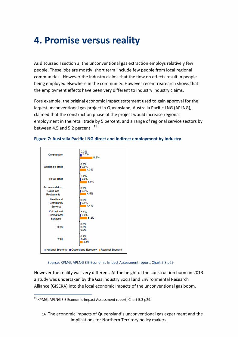
16 The economic impacts of Queensland’s unconventional gas experiment and the implications for Northern Territory policy makers.

4. Promise versus reality

As discussed I section 3, the unconventional gas extraction employs relatively few

people. These jobs are mostly short term include few people from local regional

communities. However the industry claims that the flow on effects result in people

being employed elsewhere in the community. However recent rearearch shows that

the employment effects have been very different to industry industry claims.

Fore example, the original economic impact statement used to gain approval for the

largest unconventional gas project in Queensland, Australia Pacific LNG (APLNG),

claimed that the construction phase of the project would increase regional

employment in the retail trade by 5 percent, and a range of regional service sectors by

between 4.5 and 5.2 percent . 11

Figure 7: Australia Pacific LNG direct and indirect employment by industry

Source: KPMG, APLNG EIS Economic Impact Assessment report, Chart 5.3 p29

However the reality was very different. At the height of the construction boom in 2013

a study was undertaken by the Gas Industry Social and Environmental Research

Alliance (GISERA) into the local economic impacts of the unconventional gas boom.

11

KPMG, APLNG EIS Economic Impact Assessment report, Chart 5.3 p29.

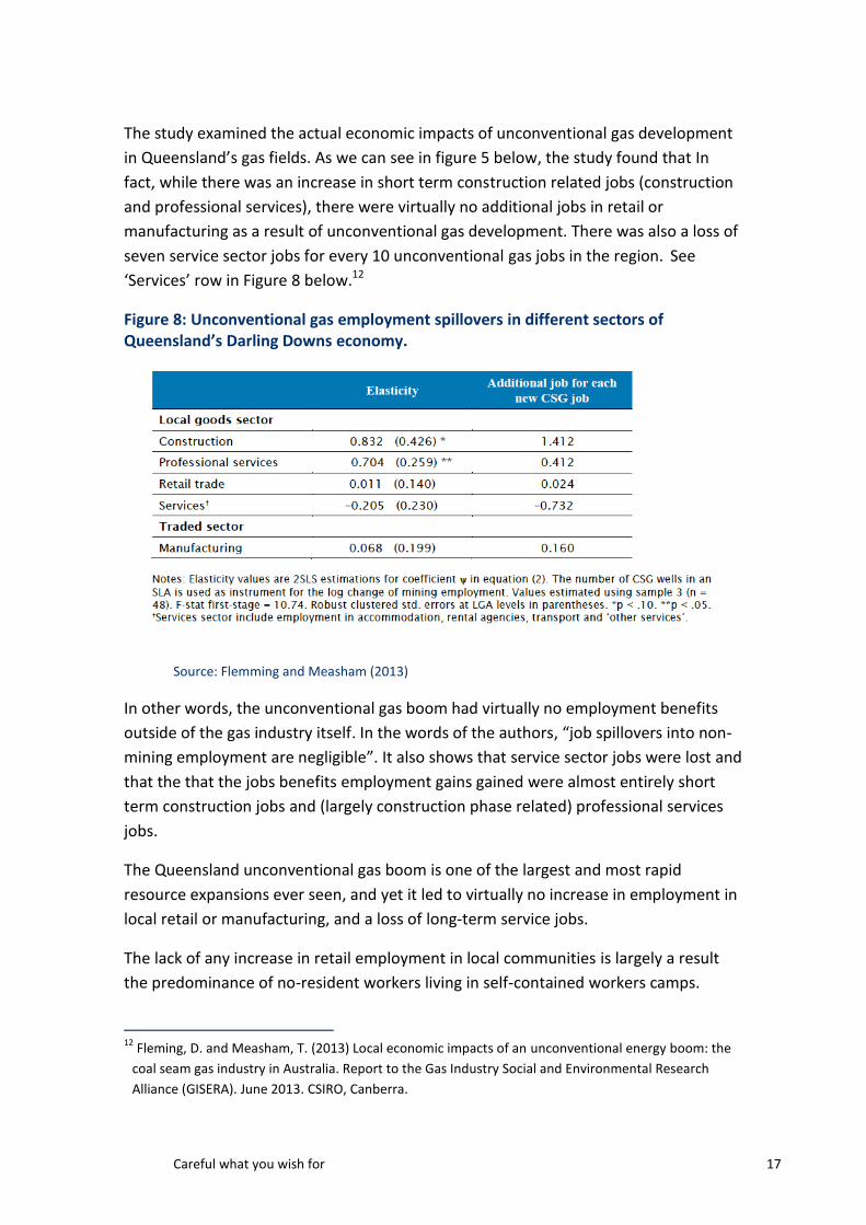
Careful what you wish for 17

The study examined the actual economic impacts of unconventional gas development

in Queensland’s gas fields. As we can see in figure 5 below, the study found that In

fact, while there was an increase in short term construction related jobs (construction

and professional services), there were virtually no additional jobs in retail or

manufacturing as a result of unconventional gas development. There was also a loss of

seven service sector jobs for every 10 unconventional gas jobs in the region. See

‘Services’ row in Figure 8 below.12

Figure 8: Unconventional gas employment spillovers in different sectors of Queensland’s Darling Downs economy.

Source: Flemming and Measham (2013)

In other words, the unconventional gas boom had virtually no employment benefits

outside of the gas industry itself. In the words of the authors, “job spillovers into non-

mining employment are negligible”. It also shows that service sector jobs were lost and

that the that the jobs benefits employment gains gained were almost entirely short

term construction jobs and (largely construction phase related) professional services

jobs.

The Queensland unconventional gas boom is one of the largest and most rapid

resource expansions ever seen, and yet it led to virtually no increase in employment in

local retail or manufacturing, and a loss of long-term service jobs.

The lack of any increase in retail employment in local communities is largely a result

the predominance of no-resident workers living in self-contained workers camps.

12

Fleming, D. and Measham, T. (2013) Local economic impacts of an unconventional energy boom: the

coal seam gas industry in Australia. Report to the Gas Industry Social and Environmental Research

Alliance (GISERA). June 2013. CSIRO, Canberra.

18 The economic impacts of Queensland’s unconventional gas experiment and the implications for Northern Territory policy makers.

These employees work long shifts that limit opportunities to spend their income in the

local community.

The lack of flow on manufacturing jobs is the result of the gas industry’s preference for

sourcing materials and equipment from overseas. For example, the huge LNG export

and processing facilities at Gladstone in Queensland were entirely designed and built

overseas.

All three export terminals were built by the global oil and gas engineering company

Bechtel. On their website, Bechtel promote their “efficiency” in not employing

Australians. The website page shown in Figure 8 describes all three of the Gladstone

LNG Processing plants and export terminals as being designed by Bechtel engineers in

Houston, Delhi and Shanghai, to be built in the Philippines, Indonesia and Thailand.

The terminals were then floated over to Australia to be assembled.13

Figure 9: Bechtel description of design and construction process for their Curtis Island LNG terminals in Queensland.

13

Bechtel website http://www.bechtel.com/projects/curtis-island-lng/ accessed 10/11/15.

Careful what you wish for 19

5. Boom and bust

According to the Office of the Chief Economist of Australia, the three unconventional

gas projects in Queensland employed 16,000 people during their brief14 construction

phase. This is falling by over 80% to 3,000 employees as the projects enter their

operational phase.15 This will represent less than 0.13% of Queensland’s total

workforce of over 2.3 million. 16

Figure 10: Queensland unconventional gas operation and construction employment.

Source: Office of the Chief Economist of Australia (2015).

The construction workforces may have been considerably smaller than reported by the

Office of the Chief Economist. The office based the numbers on “fact sheets provided

by the companies”.17 APLNG, the largest of Queensland’s LNG projects says in its

Economic Impact Assessment that “over the 11-year construction phase, there will be

an approximate average of 3,300 people working on the Australia Pacific LNG project

each year. Employment will peak from 2012 to 2014 inclusive”. This is a little over half

the number reported by the Office of the Chief Economist but would still represent

more than a two-thirds reduction in the workforce between the construction and

operational phase.

14

The length of the construction period varies between the projects. In the case the Gladstone LNG, the

construction period was 4 years. URS (2009) GLNG Economic Impact Statement. 15

Office of the Chief Economist, Resources and Energy Major Projects list April 2015. Viewed on 11

November 2015, <http://www.industry.gov.au/Office-of-the-Chief-

Economist/Publications/Pages/Resources-and-energy-major-projects.aspx> 16

ABS Labour Force Statistics. 17

Correspondence with the Office of the Chief Economist.

20 The economic impacts of Queensland’s unconventional gas experiment and the implications for Northern Territory policy makers.

Any unconventional gas project in the Northern Territory would employ far fewer

workers than in Queensland.

A large proportion of both the construction and operational workforce in Queensland

worked on assembling the LNG terminals at Gladstone. Additional LNG terminals will

not be required in the Northern Territory as the gas will be exported via the

Queensland terminals.

There is also likely to be a large pool of experienced gas workers in Western Australia

and Queensland who are well placed to fill Northern Territory unconventional gas jobs.

The three Queensland LNG terminals, the Northern Territory Inpex project and several

Western Australian LNG terminals and offshore gas fields were all built simultaneously.

The decision to allow all these projects to be built simultaneously created an acute

skills shortage at the time. With the wind down of the construction phase of these

projects there is an abundance of interstate skilled gas construction workers who will

be far better placed to work in any gas projects in the NT than unemployed NT

residents who lack these skills.

To the extent that NT residents are employed, they are likely to be skilled workers

already employed in other industries, particularly manufacturing and agriculture. This

effect drives up costs for other industries as they are forced to compete with the oil

and gas industry for skilled workers.

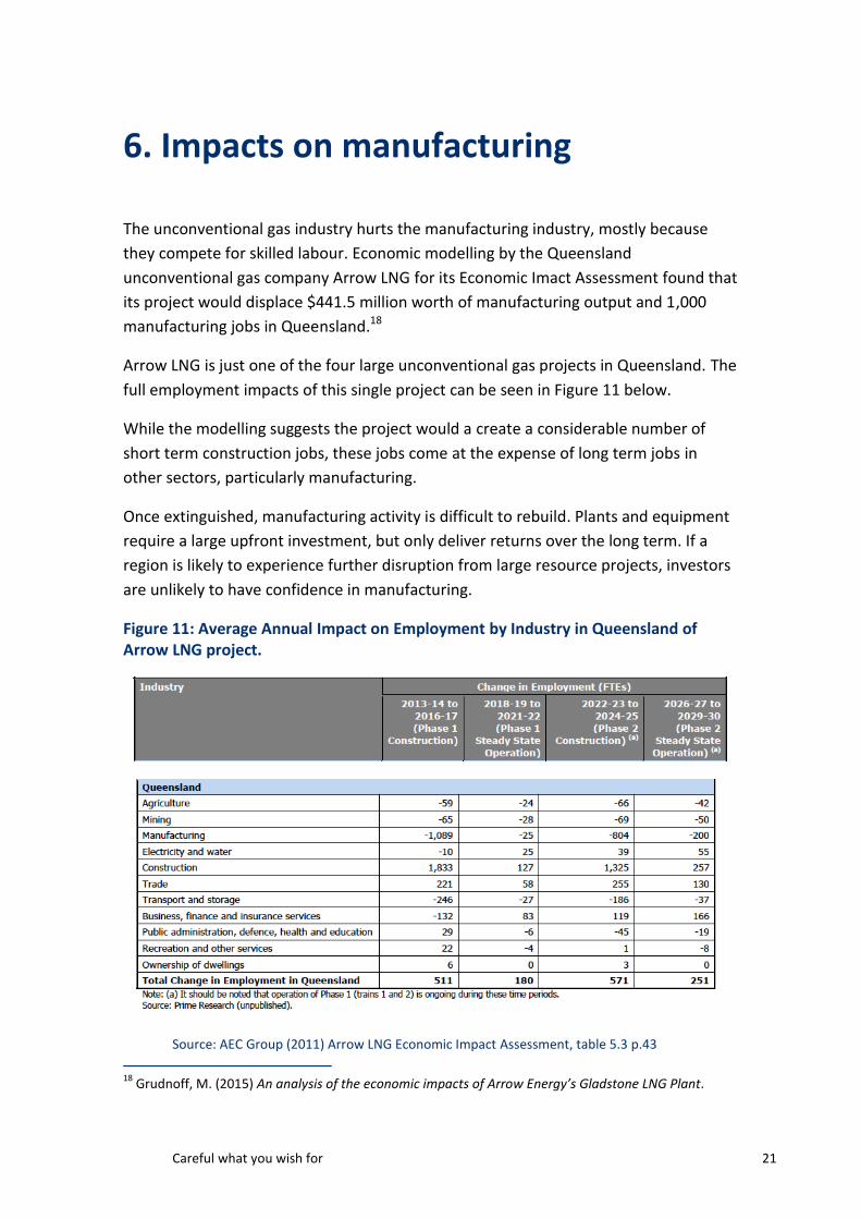
Careful what you wish for 21

6. Impacts on manufacturing

The unconventional gas industry hurts the manufacturing industry, mostly because

they compete for skilled labour. Economic modelling by the Queensland

unconventional gas company Arrow LNG for its Economic Imact Assessment found that

its project would displace $441.5 million worth of manufacturing output and 1,000

manufacturing jobs in Queensland.18

Arrow LNG is just one of the four large unconventional gas projects in Queensland. The

full employment impacts of this single project can be seen in Figure 11 below.

While the modelling suggests the project would a create a considerable number of

short term construction jobs, these jobs come at the expense of long term jobs in

other sectors, particularly manufacturing.

Once extinguished, manufacturing activity is difficult to rebuild. Plants and equipment

require a large upfront investment, but only deliver returns over the long term. If a

region is likely to experience further disruption from large resource projects, investors

are unlikely to have confidence in manufacturing.

Figure 11: Average Annual Impact on Employment by Industry in Queensland of Arrow LNG project.

Source: AEC Group (2011) Arrow LNG Economic Impact Assessment, table 5.3 p.43

18

Grudnoff, M. (2015) An analysis of the economic impacts of Arrow Energy’s Gladstone LNG Plant.

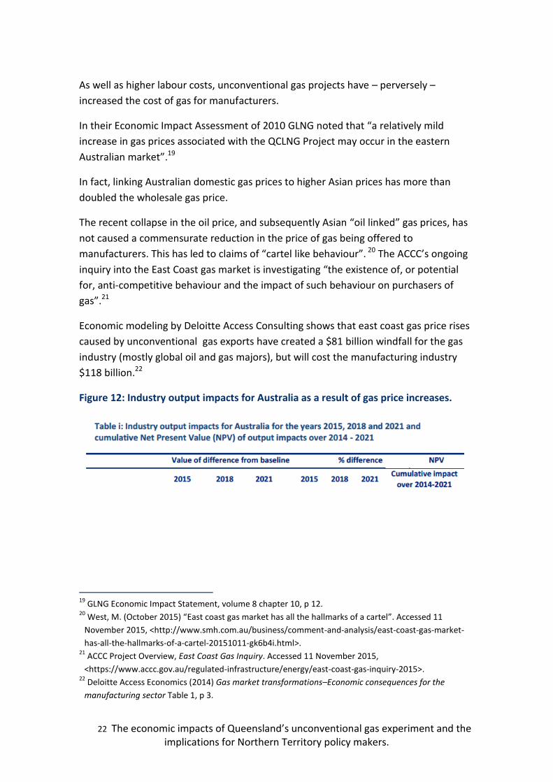
22 The economic impacts of Queensland’s unconventional gas experiment and the implications for Northern Territory policy makers.

As well as higher labour costs, unconventional gas projects have – perversely –

increased the cost of gas for manufacturers.

In their Economic Impact Assessment of 2010 GLNG noted that “a relatively mild

increase in gas prices associated with the QCLNG Project may occur in the eastern

Australian market”.19

In fact, linking Australian domestic gas prices to higher Asian prices has more than

doubled the wholesale gas price.

The recent collapse in the oil price, and subsequently Asian “oil linked” gas prices, has

not caused a commensurate reduction in the price of gas being offered to

manufacturers. This has led to claims of “cartel like behaviour”. 20 The ACCC’s ongoing

inquiry into the East Coast gas market is investigating “the existence of, or potential

for, anti-competitive behaviour and the impact of such behaviour on purchasers of

gas”.21

Economic modeling by Deloitte Access Consulting shows that east coast gas price rises

caused by unconventional gas exports have created a $81 billion windfall for the gas

industry (mostly global oil and gas majors), but will cost the manufacturing industry

$118 billion.22

Figure 12: Industry output impacts for Australia as a result of gas price increases.

19

GLNG Economic Impact Statement, volume 8 chapter 10, p 12. 20

West, M. (October 2015) “East coast gas market has all the hallmarks of a cartel”. Accessed 11

November 2015, <http://www.smh.com.au/business/comment-and-analysis/east-coast-gas-market-

has-all-the-hallmarks-of-a-cartel-20151011-gk6b4i.html>. 21

ACCC Project Overview, East Coast Gas Inquiry. Accessed 11 November 2015,

<https://www.accc.gov.au/regulated-infrastructure/energy/east-coast-gas-inquiry-2015>. 22

Deloitte Access Economics (2014) Gas market transformations–Economic consequences for the

manufacturing sector Table 1, p 3.

Careful what you wish for 23

Source: Deloitte Access Economics (2014)

No amount of additional gas extraction in the Northern Territory or elsewhere will

reduce gas prices in Australia as all gas will now go to the Asian market. As the NSW

Independent Pricing and Regulatory Tribunal (IPART) put it:

The increase in regulated retail gas prices 2014/15 reflects increased wholesale

gas costs as eastern Australia becomes part of a single global market for

commodity gas, as well as increasing network charges.23

23

Inquiry into the supply and cost of gas liquid fuels in NSW, IPART 2014. Accessed 10 July 2015,

<http://www.parliament.nsw.gov.au/prod/parlment/committee.nsf/0/efb3f0c1908f7b21ca257dc7000

5b1b 2/$FILE/0023%20-%20IPART.pdf>

24 The economic impacts of Queensland’s unconventional gas experiment and the implications for Northern Territory policy makers.

7. Big numbers, small benefits

Gas companies often cite the amount of money they invest or the value of the gas they

sell as proof of the economic benefits of their projects.

However these numbers say little about benefits for Australians if the money invested

in a project is spent on equipment from overseas, profits flow to foreign investors and

the companies pay little tax or royalties.

The oil and gas industry in Australia is over 80% foreign owned,24 which means that

over 80% of the profits go directly off shore. It imports almost all its equipment and

pays very low rates of tax. The theoretical company tax rate in Australia is 30%. All

industries are able to claim exemptions and the average effective company tax rate of

all industries in 2011/12 was 17.6%. That year the oil and gas industry in Australia paid

an effective company tax rate of 5.4%.25

The Queensland LNG projects were approved without an estimate of royalty payments

to the state government.

As the Reserve Bank of Australia concluded, while Australian production of LNG is

expected to ramp up substantially over the next few years:

The effect on Australian living standards will be less noticeable than this given

the low employment intensity of LNG production, the high level of foreign

ownership of the LNG industry and, in the near term, the use of deductions on

taxation payments. 26

The big numbers for capital value or change in GDP tell us little about the benefit of

gas exports to the wider Australian economy and community. As the Reserve Bank of

Australia notes, these benefits are likely to be smaller.

24

Calculations by The Australia Institute based on published 2P reserves and production. 25

Taxation statistics 2011–12, Table 4: Company tax, Selected items by industry, ABS

81550DO002_201112 Australian Industry. 26

Cassidy, N. and Kosev, M. (2015) Australia and the Global LNG Market, RBA.

Careful what you wish for 25

8. The Industrial footprint of shale gas

One important way that unconventional gas development differs from other types of

resource development is that it covers far greater areas. Mines are generally highly

concentrated with relatively small footprints, while unconventional gas fields often cover

tens of thousands of square kilometers with an industrial grid of wells, pipelines, access

roads, compressor stations and water treatment plants.

The most mature shale gas field in the US, the Barnett Shale has an average of 1.15

wells per square kilometer, but is as high as 6 wells per square kilometer due to “infill

drilling” needed to extract gas as fields deplete.27

Every shale gas well needs to be fracked multiple times. Every frack requires 11-34

million litres of water28 equating to 360-11,000 truckloads and “80-300 tonnes of

industrial chemicals 29. This is potentially an enormous increase in truck mvements on

the Territory’s roads and will inevitable impact other road users.

Pennsylvania in the United States has a mature shale gas industry. A gas industry

study last year in Pennsylvania found that more than 6% of gas wells leaked, and up to

75% of wells could have some form of integrity failure. 30 In Pennsylvania more than

240 private drinking water wells have been contaminated or have dried up as the

result of drilling and fracking operations over a seven-year period31

27

Shale Gas Information Platform SHIP. GFZ http://www.shale-gas-information-

platform.org/categories/operations/the-basics.html Accessed 10/11/15 28 UNEP Global Environmental Alert Service: Gas Fracking: Can we safely squeeze the rocks? 29

Hazen and Sawyer, December 22, 2009. Impact Assessment of Natural Gas Production in the New

York City Water Supply Watershed. 30

Davies, R. J., Almond, S., Ward, R. S., Jackson, R. B., Adams, C., Worrall, F., ... Whitehead, M. A. (2014).

Oil and gas wells and their integrity: Implications for shale and unconventional resource exploitation.

Marine and Petroleum Geology, 56, 239-254. doi: 10.1016/j.marpetgeo.2014.03.001 31

Concerned Health Professionals of New York & Physicians for Social Responsibility. (2015, October 14).

Compendium of scientific, medical, and media findings demonstrating risks and harms of fracking

(unconventional gas and oil extraction) (3rd ed.). http://concernedhealthny.org/compendium/

26 The economic impacts of Queensland’s unconventional gas experiment and the implications for Northern Territory policy makers.

Conclusion

Gas companies routinely exaggerate the economic and jobs benefits of their projects.

Policy makers often accept these claims unquestioningly.

The Northern Territory is fortunate to have the Queensland unconventional gas

experiment to reflect upon. The Queensland experience is that most of the economic

benefits do not materialise, and serious collateral damage is done to existing industries

and local communities.

If policy makers in the Northern Territory naively accept the economic claims of

speculative gas companies and use taxpayer money to support this industry,

Territorians will live the consequences for decades to come.