energy saving exploiting light availability: a new method ... · energy saving exploiting light...

239

Energy Saving Exploiting Light Availability: A New Method to Evaluate Daylight Contribution

Claudio Campanile – University of Pisa, DESTeC – [email protected]

Francesco Leccese – University of Pisa, School of Engineering, Dept. of Energy Engineering, Systems,

Territory and Constructions (DESTeC) – [email protected]

Michele Rocca – University of Pisa, DESTeC – [email protected]

Giacomo Salvadori – University of Pisa, DESTeC – [email protected]

Abstract Rhinoceros and Grasshopper have the extensibility which

makes architects able to study forms, structures, acoustic

behaviour, energy consumption, etc. as well as daylight

availability: the most important aspect in this study. The

software described has been useful to evaluate running

costs including heating, cooling, electrical devices and

lighting systems.

The software used includes Ladybug and Honeybee; they

connect the Radiance and Daysim engines to Grasshopper

and Rhinoceros.

The building analyzed in this study is a competition

proposal for the New Town Hall in Remseck Am Neckar

(Germany). The simulation started by designing the

electric lighting system while the daylight availability

was evaluated afterwards. The core study is the critical

investigation of the daylight contribution necessary to

satisfy the lighting demand.

Two simulations were run: the first one followed the

European Regulation EN 15193, the second one was

based on Daysim. If these methodologies gave two

equivalent results for the north-exposed offices, on the

other hand the south-exposed rooms obtained slightly

different values. The idea consists in developing a third

method to use opposed to the others described before,

called the ‘Octopus method’ (OM) and based on Octopus,

a multi-objective evolutionary algorithm integrated

within Grasshopper. The new feature the OM introduces is

the annual illuminance data computation being different

from Daysim. The latter just makes a multiplication

between the illuminance deficiency and the required

comfort level. The OM considers the comfort level

throughout the year simulating the real illuminance

distribution within the ambient of study and the effect of

electric light system installed.

1. Building Simulation: Nowadays

A critical approach is introduced to evaluate the

lighting system consumption depending on the

daylight availability – the most critical aspect

about energy demand for office buildings (Tuoni et

al., 2010; Leccese et al., 2012).

Originally, the matter of understanding and

controlling the energy demand came from the need

to check if the design proposed fulfills the

requirements.

The more complex a project is, the more the desire

to control it increases, due to the need to evaluate

costs and benefits through simulation tools

(Leccese et al., 2009; Angeli et al. 2005; Angeli et al.

2004; Lazzarotti et al. 2003).

Lately, software solutions have become more and

more advanced to satisfy professionals’ necessities

as much as possible.

The authors looked for a software environment for

having both a strong reliability and a smart user

interface to focus on the physical behaviour.

2. The choice of the software environment

The choice was Rhinoceros (RH) and Grasshopper

(GH). The software environment, thanks to its add-

on architecture, allows us to pursue aspects more

in depth than was possible until now. They have

the extensibility that makes architects able to study

daylight availability: the most important aspect in

this study.

Since both RH and GH do not include any

mailto:[email protected]

Claudio Campanile, Franscesco Leccese, Michele Rocca, Giacomo Salvadori

240

environmental tools, but just geometry and data

structure management engines, the Ladybug (LB)

and Honeybee (HB) add-ons were added to the tool

package.

For those who are not confident with this plug-in, a

brief description follows.

LB and HB are a collection of user components

developed in Python programming language

within GH by Mostapha Sadeghipour Roudsari et

al. at Thornton Tomasetti as Integration

Applications Developer. The tool connects the

Radiance and Daysim engines to Grasshopper and the

Rhinoceros 3D-environment. The software

described has been useful to evaluate running costs

of the New Town Hall building including heating,

cooling, electrical devices and lighting system

which is deeply analyzed in this study.

The RH and GH interface is well known and

generally user-friendly while the reliability has

been checked through tests conducted on already-

known conditions.

Once the tool-ecosystem is described, it is also

necessary to talk about the environmental data

source. The U.S. Department of Energy, thanks to

their database based on *.epw files (EnergyPlus

weather file format), was chosen thanks to its

intrinsic interoperability and completeness.

Consequently, input data were verified in

comparison with the Italian Regulation Weather

Data: the difference found was acceptable

(Campanile, 2014).

In addition to this, it must be said that the

reliability checking was done even for LB and HB

Radiance implementation: a test model was

processed both in DIALux and HB and then the

results were compared (Campanile, 2014). The

geometry is a simple room with one window and a

test grid able to measure the illuminance level from

a light source. Once again, difference was around

2%, which is more than acceptable.

The usage of GH and its add-ons led us to consider

the overall software reliability. Since GH lets

literally everyone able to make new open source

environmental plug-ins, this has two effects. The first

one, which is positive, is that researchers have

either a flexible, free, powerful and diffused tool to

deepen their studies. The other side of the coin is

that sometimes these software extensions do not

follow a proper reliability check and might be fine

for the purpose they was developed for, but not for

other cases. As we expected from an add-on

created by Thornton Tomasetti, the checking

results have been excellent even if LB and HB are

still a work in progress.

3. Case of study

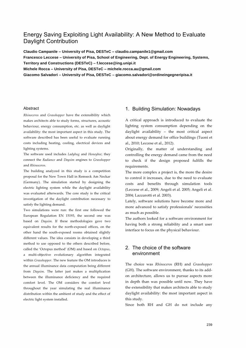
The building tested is part of a competition

proposal for the New Town Hall in Remseck Am

Neckar (Stuttgart, Germany) designed by C.

Campanile (Campanile, 2014) at MDU Architetti

(Prato, Italy), see Figs. 1-3. The buildings are glaze-

enveloped volumes which, on one hand are

strongly naturally enlightened; on the other, they

have been defined to create a strong linkage

between external and internal spaces due to the

high quality natural surrounding: the confluence of

two rivers. This has been the result of the design

research, conducted to be satisfactory in terms of

the membrane’s performance behaviour.

The analysis was run for the Town Hall Building

for two reasons: firstly, this is the most complex

building compared to the Library and the Civic

Hall (Fig. 1). On the other hand, it is actually an

office building: it is a much-diffused typology and

mostly it is affected by high-energy consumption

because of its electrical light system.

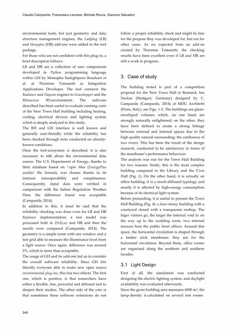
Before proceeding, it is useful to present the Town

Hall Building (Fig. 4): a four-storey building with a

courtyard closed with a transparent rooftop. The

higer visitors go, the larger the internal void is: on

the way up to the wedding room, two internal

terraces host the public front offices. Around this

space, the horizontal circulation is shaped through

a timber stick membrane: they are for the

horizontal circulation. Beyond them, office rooms

are organized along the northern and southern

facades.

3.1 Light Design First of all, the simulation was conducted

designing the electric lighting system, and daylight

availability was evaluated afterwards.

Since the gross building area measures 6000 m2, the

lamp density is calculated on several test rooms


241

and split between those exposed to the north and

those exposed to the south.

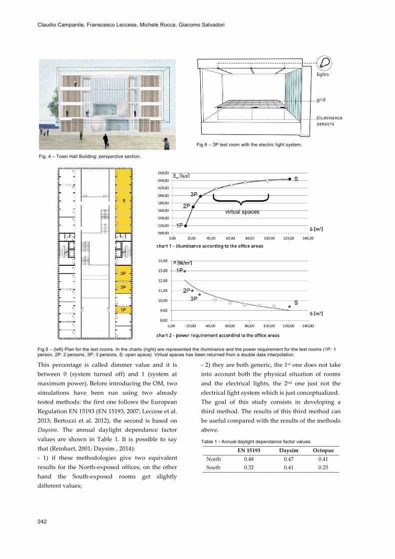
The electric light system was designed studying

four different test rooms: single (1P), double (2P),

triple (3P) and open space office (S). Then, results

were interpolated to devise a function able to

match the power needed with their areas (Fig. 5).

From this point forwards, we will consider the

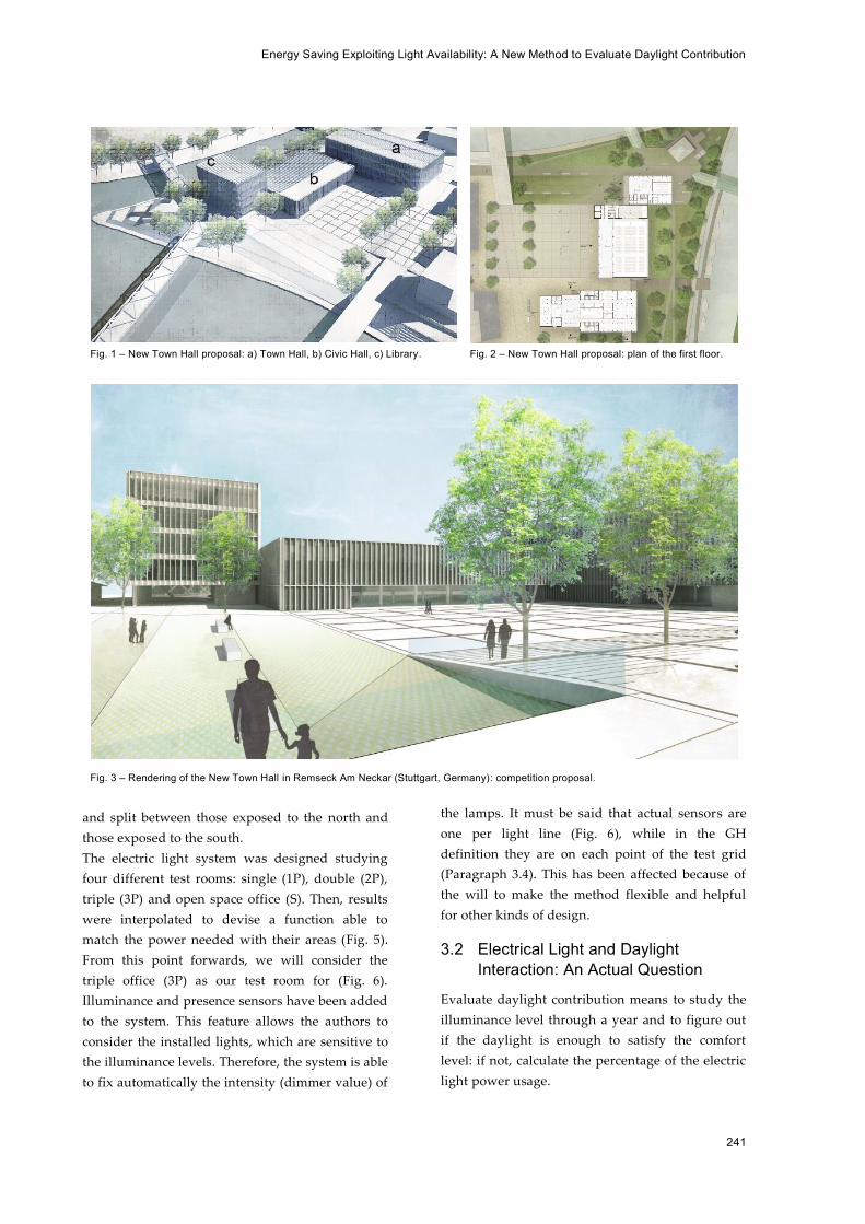
triple office (3P) as our test room for (Fig. 6).

Illuminance and presence sensors have been added

to the system. This feature allows the authors to

consider the installed lights, which are sensitive to

the illuminance levels. Therefore, the system is able

to fix automatically the intensity (dimmer value) of

the lamps. It must be said that actual sensors are

one per light line (Fig. 6), while in the GH

definition they are on each point of the test grid

(Paragraph 3.4). This has been affected because of

the will to make the method flexible and helpful

for other kinds of design.

3.2 Electrical Light and Daylight Interaction: An Actual Question

Evaluate daylight contribution means to study the

illuminance level through a year and to figure out

if the daylight is enough to satisfy the comfort

level: if not, calculate the percentage of the electric

light power usage.

Fig. 1 – New Town Hall proposal: a) Town Hall, b) Civic Hall, c) Library.

Fig. 2 – New Town Hall proposal: plan of the first floor.

Fig. 3 – Rendering of the New Town Hall in Remseck Am Neckar (Stuttgart, Germany): competition proposal.


242

Fig. 4 – Town Hall Building: perspective section.

This percentage is called dimmer value and it is

between 0 (system turned off) and 1 (system at

maximum power). Before introducing the OM, two

simulations have been run using two already

tested methods: the first one follows the European

Regulation EN 15193 (EN 15193, 2007; Leccese et al.

2013; Bertozzi et al. 2012), the second is based on

Daysim. The annual daylight dependance factor

values are shown in Table 1. It is possible to say

that (Reinhart, 2001; Daysim , 2014):

- 1) if these methodologies give two equivalent

results for the North-exposed offices, on the other

hand the South-exposed rooms get slightly

different values;

Fig 6 – 3P test room with the electric light system.

- 2) they are both generic, the 1st one does not take

into account both the physical situation of rooms

and the electrical lights, the 2nd one just not the

electrical light system which is just conceptualized.

The goal of this study consists in developing a

third method. The results of this third method can

be useful compared with the results of the methods

above.

Table 1 - Annual daylight dependance factor values.

EN 15193 Daysim Octopus

North 0.48 0.47 0.41

South 0.32 0.41 0.25

Fig.5 – (left) Plan for the test rooms. In the charts (right) are represented the illuminance and the power requirement for the test rooms (1P: 1 person, 2P: 2 persons, 3P: 3 persons, S: open space). Virtual spaces has been returned from a double data interpolation.


243

3.3 An Initial Daylight Evaluation

Since this two methods are commonly used for this

purpose, we will skip the EN 15193 one and

present briefly the second one because of it is

strongly connected to the OM. Daysim is useful to

calculate the Daylight Autonomy and has been

integrated in HB. This properly means that, when

an annual daylight study is run, it gives back the

hourly illuminance level through the whole year.

Even automatic systems and sensors are taken into

account. In this case study two functions are

considered as integrated in the system: illuminance

sensors and automatic dynamic blinds. The second

one useful for what concern the comfort, but not

influential for the OM. Once that Daysim returns

the results about illuminance levels, an

approximate system just makes a multiplication

between the illuminance deficiency and the

required comfort level. This is the way Daysim use

to "conceptualize" the electrical light system. From

this point forward it is shown how to include the

actual electrical light system into the evaluation

through the OM. It must be said that its

development is enough to use it not to substitute

the other two methods, but to help users to

understand the behavior.

3.4 The Octopus Method

The name ‘Octopus Method’ (OM) is due to the

fact that it is based on Octopus, a multi-objective

evolutionary algorithm integrated within

Grasshopper (Octopus, 2014). The new feature the

OM introduces is the annual illuminance data

computation being different from Daysim. The

latter just makes a multiplication between the

illuminance deficiency and the required comfort

level. The OM takes into account the comfort level

throughout the year simulating the actual

illuminance distribution within the ambient of

study and the real electric light system installed.

(Step 1) The OM has been run inside a test room -

once South-oriented, once North-oriented - already

designed in RH and used for the Daysim method

(Fig. 7). Since nothing changes talking about the

method, only the South-oriented room is

considered to show the OM, while both the results

will be shown. The room test is intended in this

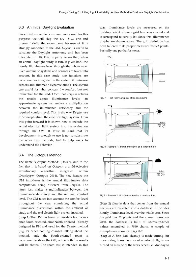
way: illuminance levels are measured on the

desktop height where a grid has been created and

it correspond to zero (0 lx). Since this, illuminance

graphs are drawn above. The grid definition has

been tailored to its proper measure: 8x9=72 points.

Basically one per half a meter.

Fig. 7 – Test room: a typical office room (3P).

Fig. 8 – Sample 1: illuminance level at a random time.

Fig.9 – Sample 2: illuminance level at a random time.

(Step 2) Daysim data that comes from the annual

analysis are collected into a database: it includes

hourly illuminance level over the whole year. Since

the grid has 72 points and the annual hours are

7860, the database is built of 72x7860=630720

values assembled in 7860 charts. A couple of

examples are shown in Figs. 8-9.

(Step 3) A first data cleanup is made cutting out

no-working hours because of no electric lights are

turned on outside of the work schedule: Monday to


244

Friday (5 days per week), 8 am to 6 pm (10 hours

per day). Holidays are not included: we will see

later that this is not conclusive, and the reason is

that the method is based on monthly average

daylight availability. At the end of this step the

data pattern is changed: only 50 out of 178 weekly

hours are included in the calculation. Since one

year is made of 52 weeks, the result is that in the

whole year only 2600 hours (charts) out of 7680 are

taken into account (and 2600x72=187200 point

values).

Within the last step, the average monthly daylight

availability (True Monthly Average, TMA) has

been introduced: the method is based on the

average since the goal is to calculate the energy

consumption. From this point forward, the

database is useless for the comfort level evaluation.

Before going further, it is appropriate to show how

the average is made up or, we could say, how we

extrapolate 12 charts (one per month) from 2600.

The TMA is calculated about the single value (grid

point) in the chart, for that charts which are

included in one month. We call it ‘true’, because

actually, to go forward into the method, we need a

Fake Monthly Average (FMA). It is so-called

because it included all the 187200 point values,

whereas it includes a condition: the values 'bigger

than the comfort level’ are considered ‘at the

comfort level’ (500 lx). The reason of this is

understandable through the following example: a

grid-point, at a certain time, has the illuminance

level at 200 lx. The same point, at another certain

time, has the illuminance level at 800 lx. The

average is (200+800)/2=500 lx, i.e. the comfort level.

The average shows that no electrical light is

required, while actually, it is. Since this thought,

we can proceed as it follows.

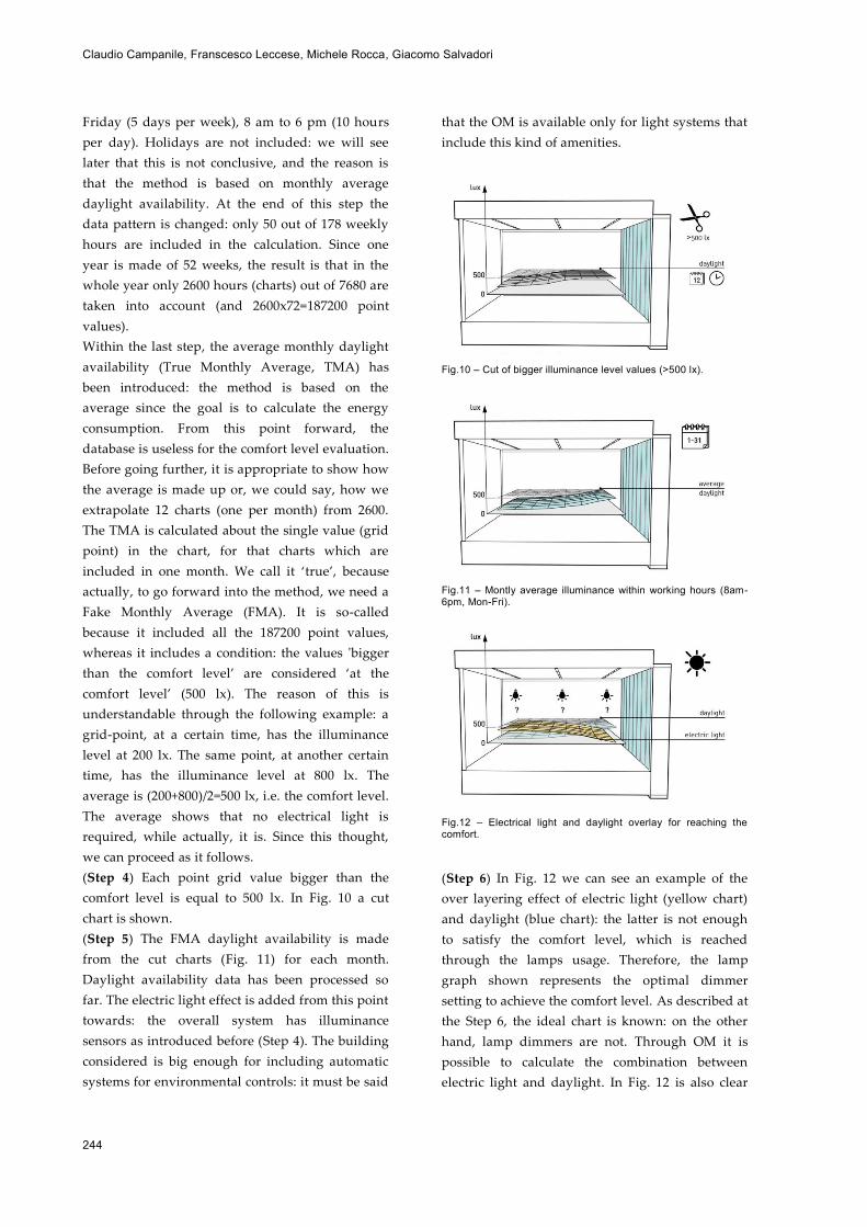
(Step 4) Each point grid value bigger than the

comfort level is equal to 500 lx. In Fig. 10 a cut

chart is shown.

(Step 5) The FMA daylight availability is made

from the cut charts (Fig. 11) for each month.

Daylight availability data has been processed so

far. The electric light effect is added from this point

towards: the overall system has illuminance

sensors as introduced before (Step 4). The building

considered is big enough for including automatic

systems for environmental controls: it must be said

that the OM is available only for light systems that

include this kind of amenities.

Fig.10 – Cut of bigger illuminance level values (>500 lx).

Fig.11 – Montly average illuminance within working hours (8am-6pm, Mon-Fri).

Fig.12 – Electrical light and daylight overlay for reaching the comfort.

(Step 6) In Fig. 12 we can see an example of the

over layering effect of electric light (yellow chart)

and daylight (blue chart): the latter is not enough

to satisfy the comfort level, which is reached

through the lamps usage. Therefore, the lamp

graph shown represents the optimal dimmer

setting to achieve the comfort level. As described at

the Step 6, the ideal chart is known: on the other

hand, lamp dimmers are not. Through OM it is

possible to calculate the combination between

electric light and daylight. In Fig. 12 is also clear


245

that the yellow chart can be affected by lower

dimmer on the window side (right) and bigger

values on the wall side (left).

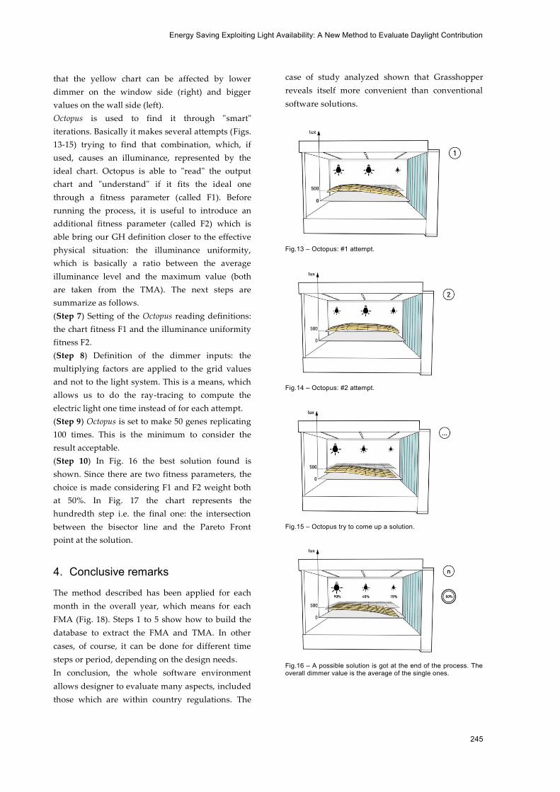
Octopus is used to find it through "smart"

iterations. Basically it makes several attempts (Figs.

13-15) trying to find that combination, which, if

used, causes an illuminance, represented by the

ideal chart. Octopus is able to "read" the output

chart and "understand" if it fits the ideal one

through a fitness parameter (called F1). Before

running the process, it is useful to introduce an

additional fitness parameter (called F2) which is

able bring our GH definition closer to the effective

physical situation: the illuminance uniformity,

which is basically a ratio between the average

illuminance level and the maximum value (both

are taken from the TMA). The next steps are

summarize as follows.

(Step 7) Setting of the Octopus reading definitions:

the chart fitness F1 and the illuminance uniformity

fitness F2.

(Step 8) Definition of the dimmer inputs: the

multiplying factors are applied to the grid values

and not to the light system. This is a means, which

allows us to do the ray-tracing to compute the

electric light one time instead of for each attempt.

(Step 9) Octopus is set to make 50 genes replicating

100 times. This is the minimum to consider the

result acceptable.

(Step 10) In Fig. 16 the best solution found is

shown. Since there are two fitness parameters, the

choice is made considering F1 and F2 weight both

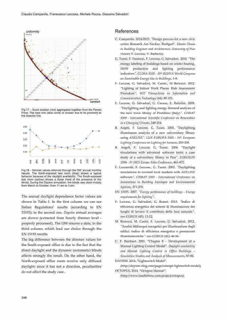
at 50%. In Fig. 17 the chart represents the

hundredth step i.e. the final one: the intersection

between the bisector line and the Pareto Front

point at the solution.

4. Conclusive remarks

The method described has been applied for each

month in the overall year, which means for each

FMA (Fig. 18). Steps 1 to 5 show how to build the

database to extract the FMA and TMA. In other

cases, of course, it can be done for different time

steps or period, depending on the design needs.

In conclusion, the whole software environment

allows designer to evaluate many aspects, included

those which are within country regulations. The

case of study analyzed shown that Grasshopper

reveals itself more convenient than conventional

software solutions.

Fig.13 – Octopus: #1 attempt.

Fig.14 – Octopus: #2 attempt.

Fig.15 – Octopus try to come up a solution.

Fig.16 – A possible solution is got at the end of the process. The overall dimmer value is the average of the single ones.


246

Fig.17 – Good solution (red) aggregated together from the Pareto Front. The best one (blue circle) is chosen due to its proximity to the bisector line.

Fig.18 – Dimmer values returned through the OM: annual monthly results. The North-exposed test room (blue) shows a typical behavior because of the daylight availability. The South-exposed test room (yellow) shows a linear trend of the presence of the blinds. During the Daysim simulation, the blinds was down mostly from March to October, from 11 am to 3 pm.

The annual daylight dependance factor values are

shown in Table 1. In the first column we can see

Italian Regulations’ results (according to EN

15193); in the second one, Daysim annual averages

are shown (extracted from hourly dimmer level -

properly processed). The OM returns a data, in the

third column, which lead our choice through the

EN 15193 results.

The big difference between the dimmer values for

the South-exposed office is due to the fact that the

direct daylight and the dynamic (automatic) blinds

affects strongly the result. On the other hand, the

North-exposed office room receive only diffused

daylight: since it has not a direction, peculiarities

do not affect the study case.

References C. Campanile. 2014/2015. "Design process for a new civic

centre Remseck Am Neckar, Stuttgart". Master Thesis

in Building Engineer and Architecture, University of Pisa

(tutors: F. Leccese, V. Barberis).

G. Tuoni, F. Fantozzi, F. Leccese, G. Salvadori. 2010. "The

energy labeling of buildings based on winter heating,

DHW production and lighting performance

indicators". CLIMA 2010 - 10th REHVA World Congress

on Sustainable Energy Use in Buildings, 1-8.

F. Leccese, G. Salvadori, M. Casini., M Bertozzi. 2012.

"Lighting of Indoor Work Places: Risk Assessment

Procedure". WIT Transactions on Information and

Communication Technology (44): 89-101.

F. Leccese, G. Salvadori, G. Caruso, E. Batistini. 2009.

"Daylighting and lighting energy demand analysis of

the new town library of Piombino (Italy)". CISBAT

2009 - International Scientific Conference on Renewables

in a Changing Climate, 249-254.

B. Angeli, F. Leccese, G. Tuoni. 2005. "Daylighting

illuminance analysis of a new universitary library

using ADELINE". LUX EUROPA 2005 - 10th European

Ligthing Conference on Lighting for humans, 205-208.

B. Angeli, F. Leccese, G. Tuoni. 2004. "Daylight

simulations with advanced software tools: a case

study of a universitary library in Pisa". EUROSUN

2004 - 5th ISES Europe Solar Conference, 463-472.

F. Lazzarotti, F. Leccese., G. Tuoni. 2003. "Daylighting

simulations in covered local markets with ADELINE

software". CISBAT 2003 - International Conference on

Innovations in Building Envelopes and Environmental

Systems, 271-276.

EN 15193. 2007. "Energy performance of buildings - Energy

requirements for lighting".

F. Leccese, G. Salvadori, G. Romei. 2013. "Indice di

efficienza energetica dei sistemi di illuminazione dei

luoghi di lavoro: il contributo della luce naturale".

neo-EÚBIOS (45): 13-22.

M. Bertozzi, M. Casini, F. Leccese, G. Salvadori. 2012.

"Analisi fabbisogni energetici per illuminazione degli

edifici: indice di efficienza energetica e prestazioni

illuminotecniche". neo-EÚBIOS (41): 46-56.

C. F. Reinhart. 2001. “Chapter 8 – Development of a

Manual Lighting Control Model”. Daylight availability

and Manual Lighting Control in Office Buildings –

Simulation Studies and Analysis of Measurements, 87-96.

DAYSIM. 2014. “Lightswitch Model”.

(http://daysim.ning.com/page/concept-lightswitch-model).

OCTOPUS. 2014. “Octopus Manual”.

(http://www.food4rhino.com/project/octopus).

http://daysim.ning.com/page/concept-lightswitch-model

energy saving exploiting light availability: a new method ... · energy saving exploiting light...

Documents