ENERGY SAVINGS OBTAINED USING THE ONLINE AUTOMATIC TUBE CLEANING SYSTEM IN HVAC SYSTEMS IN AUSTRALIA: REAL WORLD CASE REVIEWS

D.P. Ross1, P.A. Cirtog1 and A. Swanson1

1 Pangolin Associates, 46 Magill Road, Norwood 5067 South Australia (davide.ross@pangolinassociates.com)

ABSTRACT Due to the very steep retail electricity prices rises of over 60% during the last 5 years, combined with increasing incidences of extreme hot weather events in Australia, having a well tuned and efficient HVAC system is paramount to meeting these challenges. The successful operation of water-cooled HVAC chillers require controlling the growth of biofilm and deposition of scale on the internal tubes of heat exchange surfaces. This reduces heat transfer efficiency and subsequently increases chiller work loads and energy consumption. Despite the extensive literature on this subject, there is ignorance and resistance in Australia to the adoption of non-chemical cleaning techniques to reduce fouling and associated operation and maintenance costs with net improvement to the Coefficient of Performance (COP) of HVAC plant. This paper presents case studies of energy savings obtained using a sponge ball Automatic Tube Cleaning System (ATCS). By using hydro mechanical principals, the system circulates sponge balls through the condenser water tubes in preset 30-minute intervals. The physical results from the installation of an ATCS are revealed when annual AS/NZS-3788 pressure equipment inspections and/or “expected” maintenance tube cleans are performed. Furthermore, comparing chiller performance before and after ATCS installation has shown a minimum 24.5% reduction in electrical energy consumption of the chillers. INTRODUCTION The importance of the Refrigeration and Air Conditioning (RAC) industry in Australia is demonstrated by the statistics estimated in Table 1. The total RAC spending estimated in Table 1 is equivalent to 1.7% of Australia’s $1.57 trillion GDP (DCCEE, 2012). Total energy consumption in all commercial buildings in Australia was estimated to have been 142.7 PJ in 2012 (Brodribb et al., 2013). Analysis of the energy consumption by end-use has determined that HVAC energy use in commercial buildings ranges from 40% to 52% of the total. This estimate was based on reviewing the energy consumption records and energy audits of more than 5,600 buildings with a total non-residential non-industrial floor space in 2009 of approximately 143.3 million square metres. Chillers are usually the single largest user of electricity in most commercial and institutional HVAC facilities.

Table 1. Economic indicators and general contributions of the RAC industry activity in Australia in 2012 [1].

Expenditure categories Economic spend ($AUD Billion)

New Hardware cost installed $5.9 Annual refrigerant cost $0.5

Energy cost $14.1 Discounted wages cost $5.7

Total 45+ million installations

22% of National electricity consumption

11% of national GHG emissions

$26.2

In many cases, they are the single largest user of any form of energy in buildings. For these reasons, maintenance and engineering managers looking for ways to improve the energy efficiency of their buildings should start by improving the efficiency of chillers. Managers have three primary options to improving chiller performance: replacement, control strategies and maintenance. As chillers are required to reject heat to complete the vapour-compression cycle, a condenser heat exchanger is used which allows heat to migrate from the refrigerant gas to either water or air. Heat transfer has the greatest single effect on chiller performance. Large chillers can have more than five miles of condenser and evaporator tubes, therefore high heat transfer is fundamental to maintaining efficiency (Piper, 2006). Water-cooled chillers incorporate the use of cooling towers, which improve the chillers' thermodynamic effectiveness as compared to air-cooled chillers. One of the most common types of water-cooled refrigerant condensers is the shell-and-tube, where the chiller refrigerant condenses outside the tubes and the cooling water circulates through the tubes in a single or multi-pass circuit. The tubes can come with enhanced internal heat transfer features and may include longitudinal or spiral grooves and ridges, internal fins, and other devices to promote turbulence and augment heat transfer. An almost unavoidable consequence of using water is that fouling of the heat exchanger surface may result from sediment, biological growth, or corrosive products.

Scale will also result from the deposition of minerals from the cooling water on the warmer surface of the condenser tube. Fouling is generally classified into the following five categories: (i) particulate, (ii) precipitation, (iii) corrosion, (iv) biofouling and (v) chemical reaction (Bott, 1995). The impacts of fouling on heat transfer surfaces is generally considered in the design of heat exchangers by using a so-called “fouling factor” in the calculation of the overall heat transfer coefficient, U. Fouling will reduce the overall heat transfer coefficient and thus leads to the reduction of the heat duty of an existing heat exchanger or to additional surface area requirements in the design of new heat exchangers. The prevalence of fouling in heat exchangers has been clearly demonstrated by several surveys that have reported that more than 90% of industrial heat exchangers suffer from fouling problems (Muller-Steinhagen, 2011; Steinhagen et al., 1992; Garrett-Price et al.,1985). When a water-cooled condenser is selected, anticipated operating conditions, including water and refrigerant temperatures, have usually been determined. Standard practice allows for a fouling factor in the selection procedure. The major uncertainty is which fouling factor to choose for a given application or water condition to obtain expected performance from the condenser. As fouling is a major unresolved problem, it is a normal practice to oversize the heat transfer surface area to account for fouling. This oversizing is normally of the order of 20%–40% (Kuppan, 2000). The Tubular Exchanger Manufacturers Association (TEMA, 1988) is the generally referenced source of fouling factors used in the design of heat exchangers. A “standard” industry fouling value of 44 mm2·K/W for condenser ratings is used (ASHRAE, 2000); however, in many cases, the values are much greater than necessary.

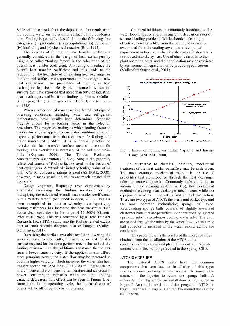
Design engineers frequently over compensate by arbitrarily increasing the fouling resistance or by multiplying the calculated overall heat transfer coefficients with a “safety factor” (Muller-Steinhagen, 2011). This has been exemplified in practice whereby over specifying fouling resistances has increased the heat transfer surface above clean conditions in the range of 20–300% (Garrett-Price et al.,1985). This was confirmed by a Heat Transfer Research, Inc. (HTRI) study into the fouling-related excess area of 2000 recently designed heat exchangers (Muller-Steinhagen, 2011). Increasing the surface area also results in lowering the water velocity. Consequently, the increase in heat transfer surface required for the same performance is due to both the fouling resistance and the additional resistance that results from a lower water velocity. If the application can afford more pumping power, the water flow may be increased to obtain a higher velocity, which increases the water film heat transfer coefficient (ASHRAE, 2000). As fouling builds up in a condenser, the condensing temperature and subsequent power consumption increases while the unit cooling capacity decreases. This effect can be seen in Figure 1. At some point in the operating cycle, the increased cost of power will be offset by the cost of cleaning.

Chemical inhibitors are commonly introduced to the water loop to reduce and/or mitigate the deposition rates of selected fouling problems. While chemical cleaning is effective, as water is bled from the cooling tower and or evaporated from the cooling tower, there is continual requirement to top up the chemical dosage as fresh water is introduced into the system. Use of chemicals adds to the plant operating costs, and their application may be restricted by environmental legislation or by product specifications (Muller-Steinhagen et al., 2011).

Fig. 1 Effect of Fouling on chiller Capacity and Energy Usage (ASHRAE, 2000)

As alternative to chemical inhibitors, mechanical treatment of the heat exchange surface may be undertaken. The most common mechanical method is the use of projectiles that are propelled through the heat exchanger tubes to remove deposits. Commonly referred to as an automatic tube cleaning system (ATCS), this mechanical method of cleaning heat exchanger tubes occurs while the equipment remains in operation and in full production. There are two types of ATCS: the brush and basket type and the more common recirculating sponge ball type. Recirculating sponge balls consists of slightly oversized elastomer balls that are periodically or continuously injected upstream into the condenser cooling water inlet. The balls are passed through the tubes by the water flow. A strainer or ball collector is installed at the water piping exiting the condenser. This paper presents the results of the energy savings obtained from the installation of the ATCS to the condensers of the centralised plant chillers of four A grade commercial office buildings located in the Sydney CBD.

ATCS OVERVIEW The featured ATCS units have the common components that constitute an installation of this type; injector, strainer and recycle pipe work which connects the strainer to the injector to return the sponge balls. A schematic flow layout for an installation is highlighted in Figure 2. An actual installation of the sponge ball ATCS for Case 1 is shown in Figure 3. In the foreground the injector can be seen.

In the background is the strainer with connecting pipework coming to the foreground. Usually, the sponge balls are 1mm larger in diameter than the I.D. of the condenser tube. The exceptions to this rule were for Case 1 and 4 due to operational issues. For Case 1, approximately 1 year after the ATCS was installed, all the plant room pump motors (primary and secondary chilled water, condenser) were fitted with variable speed drives (VSD). In particular for the condenser water pump, the drop in frequency to below 28Hz resulted in an almost 50% reduction to the water velocity through the tubes. Consequently, this meant soon after the sponge ball projectiles were injected, they became stuck within the tubes due to insufficient pressure to overcome the resistance as the balls shear the interior of the tube walls. The ideal approach to remedy this matter should have been updating the Building Management System (BMS) in order to co-ordinate the ramping up of the frequency to 50Hz (full load) for several minutes in sequence with the 30 minute injection cycles of the ATCS.

Fig. 2 ATCS design layout Alternatively, as the demonstrated stand alone savings of the ATCS solution are far superior to the savings from using a VSD on the condenser pump loop, maintaining the frequency at 50Hz would be a simple solution. This effectively eliminates the energy savings benefits of the VSD on this pump but ensures full flow through tubes. Ultimately, the plant manager utilised 1mm diameter smaller balls as a quick fix to the problem. This status quo has remained in place ever since. For Case 4, as part of an energy efficiency program to improve the efficiency star rating of the building, two new PowerPax chillers connected to a common condensing water header were installed on site in 2011. These chillers have split two-pass condenser vessel and are designed this way to avoid the expenses of a crane lift as smaller components allow access via service lifts during installation. The building’s older Trane chillers were also equipped with the ATCS and had operated without issue since installation in 2009. The building management purchased two additional ATCS units to be installed onto the PowerPax chillers in August 2013.

Some gasket interference at the midway junction of the tube rows was anticipated from prior installation experiences with the same chiller type. Previously, the gasket between the split condenser vessel had moved and become misaligned leading to partial blockage of the tubes at the time of chiller re-assembly on site. The installer raised concerns of tube misalignment during manufacturing between the two vessel halves, however the PowerPax engineer had assured this would not occur.

Fig. 3 The sponge ball ATCS installed in Case 1 As matter of precaution the condenser tubes in the middle row underneath the two-pass junction were inspected at the time of installation. Videoscope inspection showed that gasket misalignment had indeed partly block 4 of the tubes as shown in Figure 4. To remedy the gasket problem, a special hole-punch tool was used to clear the protruding gasket material to smooth the bore of the tube.

Fig. 4 Gasket misalignment in Case 4

!

Two weeks after commissioning, it was observed that none of the 20 balls were circulating through the system. Further detailed videoscope inspection was then conducted from both condenser ends of every tube in the vessel. It was subsequently found that centerline of 12 tubes were in fact misaligned causing entrapment of the balls at the junction interface of the two condenser vessel halves. To confirm the misalignment, an attempt to pass the connection point in those tubes using the gasket punch tool was tested. All attempts failed. A new set of balls (Ø 15mm) was inserted into the system. These smaller sponge balls replaced the existing sized balls that were now 1mm smaller in diameter than the 16 mm I.D. of the tube. The standard operating procedure for the injector is to hold the equivalent number of sponge balls equal to a third of the number of tubes in a single pass. Sponge balls are released from the injector on set intervals of every 30 minutes. The sponge balls ought to be replaced every 1000 hours of chiller run time. In practice, this may not occur if the site has poor maintenance scheduling. Table 2 summarises key aspects for each Case number. METHODOLOGY

The following evaluation of the energy related savings from the installation of the sponge ball ATCS has adopted the framework of the International Performance Measurement & Verification Protocol (IPMVP). For all four case studies reported here, Option C: “Whole Facility” method was used to assess the energy performance via a localised utility sub meter at the plant room sub-distribution board (IPMVP, 2012). Therefore, additional loads such as the primary and secondary chilled water pumps, condensing water pump, cooling tower fans, natural gas boiler and ventilation fans will also constitute a varying portion of the load intrinsic to each site’s plant room electrical set up. These other loads may be both static or variable in nature and are defined as the base-load energy consumption.

Table 2. A summary of the ATCS Case studies 1 to 4

The dominant independent variable on cooling load is the outside weather. Weather has many dimensions, but for whole-facility analysis, the outside air temperature is sufficient. The standard practice of using a referenced base temperature cooling degree day (CDD) was used in the present study. Cooling degree days are based on the average daily temperature. The average daily temperature is calculated as follows: [maximum daily temperature + minimum daily temperature] / 2. As HVAC load is seasonal, one full cycle is required for analysis thus, a minimum of 12 months. As all four buildings are commercially leased office spaces, potential fluctuating occupancy levels would naturally impact HVAC energy consumption. Ideally such data ought to be included into the evaluation but this was omitted due to lack of information from the building owners. Degree days are a simplified form of historical weather data - outside air temperature data relative to a base temperature, and provide a measure of how much, and for how long, the outside temperature was above that base temperature. In degree-day theory, the base temperature is effectively the "balance point" of a building when the outside temperature is below which the building does not require cooling. Naturally different buildings will have different base temperatures depending on its thermal performance. The thermal performance of a building depends on a large number of factors. They can be summarised as (i) design variables (geometrical dimensions of building elements such as walls, roof and windows, orientation, shading devices, surrounding environment etc.); (ii) material properties (density, specific heat, thermal conductivity, transmissivity, etc.); (iii) weather data (solar radiation, ambient temperature, wind speed, humidity, etc.); and (iv) a building’s usage data (internal heat gains) due to occupants, lighting, IT equipment, air exchanges, etc. In theory, dividing the energy consumption by the degree days factors out the effect of outside air temperature and enables a like-for-like comparison of energy consumption from different periods or places with different weather conditions.

Case 1 Case 2 Case 3 Case 4 No. floors 24 32 20 25

Building type Category A office building

Category A office building

Category A office building

Category A office building

NABERS energy rating 3.5 4.5 4.5 3.5 Net Lettable Area - 39,398 26,271 -

No. Chillers installed with ATCS 2 2 3 2

Chiller Make/ Trane Carrier/Trane 3 x Trane 2 x Powerpax Condenser Type Double pass Double/single pass Double pass Double pass -split

system Tube I.D. (mm) 15 22; 15 2x 22; 1x 15 16 ATCS unit size 2 x 6" 10"/6" 2 x 10" / 1 x 6" 1x 12"

Date of installation 04/2010 & 10/2010 12/2008 06/2010 08/2013

For this analysis, a reference base temperature of 18oC was used. Climate data was referenced from the Sydney Observatory Hill, weather station ID 94768 (151.21E,33.86S). A summary of the yearly CDD between 2007 and 2014 and the 10-year average (2004-2014) is summarised in Table 3. A simple linear model was used to correlate energy consumption without any adjustments, to a single independent variable, CDD. Daily CDD data is summed into monthly totals. Energy consumption is then computed such that the best fit linear regression equations fitted to the baseline and post ATCS installation data are multiplied by the 10 year average degree-day value for the corresponding month as displayed in Figure 5.

Table 3. Yearly CDD (2007-2014) and ten year average

Year CDD Variation from average

2007 801 2% 2008 661 -16% 2009 829 5% 2010 820 4% 2011 746 -5% 2012 701 -11% 2013 864 10% 2014 822 5%

10 year average 787 Standard deviation of

the mean 24.9

CV of the mean 3%

Fig. 5 Ten year monthly average CDD for Sydney CBD

The difference between the adjusted baseline and the post ATCS normalised consumption totals is the normalised energy saving. Known limitations with degree-day analysis of monthly figures, such as intermittent cooling during business office hours can also introduce a calendar mismatch.

Although monthly degree days cover the entire month, the proportion of working days for which a building is cooled does depends on the calendar of the month in question. When the inclusion of public holidays and possible shutdown periods are considered, the effect of this calendar mismatch becomes more pronounced, and degree-day analysis is also affected. In the present study, this element was not considered.

RESULTS AND DISCUSSION Figure 6 summaries the year to year monthly electricity

consumption data for the four buildings. A comparison of the energy consumption versus CDD for all four commercial office buildings is displayed in Figure 7. In all cases there was an observed reduction in net energy consumption following installation of the ATCS. The normalised energy savings using the ten year average CDD resulted in a decrease ranging between 24.5% to 26.5%. These results compare favourably with theoretical and experimental results reported by Lee and Karng (2002) for a similar sponge ball ATCS. For fouling predicted using the Kern-Seaton equation (Kern et al., 1959) the authors determined a predicted theoretical maximum energy saving for the ATCS of 28%, with an average energy saving of 24%. Their field data measured a saving of 26% for the year.

Results for Case 1 were also uniquely affected by additional energy conservation measures post the ATCS installation. As discussed, this initiative saw the installation of VSD to the numerous pump motors in the plant room, including the condenser water pump. In order to segregate the impact of the introduction of the various energy conservation measures, the post ATCS data was further separated to pre and post VSD installation. Naturally further savings were anticipated. In order to fully validate this generalised observation, a comprehensive energy audit with individual unit sub metering would be required to segregate energy use by equipment category.

The results for Case 3 were impacted by several events. The energy savings anticipated for the summer months of December 2010 to February 2011 were below expectations. Following a basic investigation it was identified that the ATCS was not serviced as required since commissioning in June 2010 by the mechanical service contractor. The major factor being the non-replacement of the sponge balls at the maximum of every 1000 hours of chiller operation. At the very most, a fifteen minute task.

New sets of balls were inserted into the system on March 2011. In May 2011, the Investa Property group acquired the site from ING property which, affected the service regime due to a change in the site mechanical contractor. A new service regime was established in September 2011 and maintained since then on a regular basis. As the ATCS system was an unknown process to the new contractor, the facility manager instigated a simplified verification evaluation to prove the imputed electrical saving was the result of the ATCS. A trial was conducted whereby all three ATCS systems were switched off for a one month period, from the 1st of February until the 1st of March 2012. The systems were back in service on the 1st March 2012.

0"

20"

40"

60"

80"

100"

120"

140"

160"

180"

Jan" Feb" Mar" Apr" May" Jun" Jul" Aug" Sep" Oct" Nov" Dec"

Cooling'degree'days/month'(CDD'ref'to'18oC)'

Fig 6 Yearly electricity consumption profiles for Cases 1 to 4

Fig 7 Monthly consumption versus CDD for Cases 1 to 4

0"

50,000"

100,000"

150,000"

200,000"

250,000"

300,000"

350,000"

Jan" Feb" Mar" Apr" May" Jun" Jul" Aug" Sep" Oct" Nov" Dec"

Electricity)consum

p0on

(kWh/yr))

Case)1)2007"

2008"

2009"

2010"

2011"

2012"

2013"

2014"

0"

20,000"

40,000"

60,000"

80,000"

100,000"

120,000"

140,000"

Jan" Feb" Mar" Apr" May" Jun" Jul" Aug" Sep" Oct" Nov" Dec"

Electricity)Co

nsum

p1on

)(kWh/yr))

Case)2)

2007"

2008"

2009"

0"

20,000"

40,000"

60,000"

80,000"

100,000"

120,000"

140,000"

160,000"

Jan" Feb" Mar" Apr" May" Jun" Jul" Aug" Sep" Oct" Nov" Dec"

Electricity)Co

nsum

p1on

)(kWh/yr))

Case)3)

2008"

2009"

2010"

2011"

2012"

2013"

0"

10000"

20000"

30000"

40000"

50000"

60000"

70000"

80000"

Jan" Feb" Mar" Apr" May" Jun" Jul" Aug" Sep" Oct" Nov" Dec"

Electricity)Co

nsum

p1on

)(kWh/yr))

Case)4)

2012"

2013"

2014"

2015"

y"="968.13x"+"142589"R²"="0.88421"

y"="898.16x"+"96494"R²"="0.8841"

y"="796.49x"+"88034"R²"="0.84184"

0"

50,000"

100,000"

150,000"

200,000"

250,000"

300,000"

350,000"

0" 20" 40" 60" 80" 100" 120" 140" 160" 180" 200"

Consum

p(on

)kWh/mon

th)

Cooling)Degree)Days)(CCD)Ref)to)18oC))

Case)1)=)24.5%)Savings)(31.9%)+)VSDs))

No"BallTech"

With"BallTech"

With"BallTech"and"VSD"

Linear"(No"BallTech)"

Linear"(With"BallTech)"

Linear"(With"BallTech"and"VSD)"

y"="605.81x"+"30047"R²"="0.83236"

y"="558.14x"+"14831"R²"="0.95893"

0"

20,000"

40,000"

60,000"

80,000"

100,000"

120,000"

140,000"

0" 20" 40" 60" 80" 100" 120" 140" 160" 180"

Consum

p(on

)(kWh/mon

th))

Cooling)degree)days)(CDD)ref)to)18oC)))

Case)2)>)26.3%)Savings)

No"BallTech"

With"BallTech"

Linear"(No"BallTech)"

Linear"(With"BallTech)"

y"="730.12x"+"26440"R²"="0.93543"

y"="647.45x"+"27954"R²"="0.93508"

y"="509.38x"+"21209"R²"="0.80006"

0"

20,000"

40,000"

60,000"

80,000"

100,000"

120,000"

140,000"

160,000"

180,000"

0" 20" 40" 60" 80" 100" 120" 140" 160" 180" 200"

Consum

p(on

)(kWh/mon

th))

Cooling)degree)days)(CDD)ref)to)18oC))

Case)3)>)26.5%)Savings)

No"Balltech"

With"BallTech"

Post"New"Balls"

Linear"(No"Balltech)"

Linear"(With"BallTech)"

Linear"(Post"New"Balls)"

y"="297.79x"+"19304"R²"="0.94007"

y"="240.88x"+"13097"R²"="0.94295"

0"

10,000"

20,000"

30,000"

40,000"

50,000"

60,000"

70,000"

80,000"

0" 20" 40" 60" 80" 100" 120" 140" 160" 180" 200"

Consum

p(on

)(kWh/mon

th))

Cooling)degree)days)(CDD)ref)to)180C))

Case)4)?25.6%)Savings)

no"balltech"

with"balltech"

Linear"(no"balltech)"

Linear"(with"balltech)"

In Cases 1 and 4 where the smaller diameter projectiles have replaced the standard sizing, the results presented here indicate this has not materially impacted the savings achieved with the ATCS. Intuitively, some reduction in efficiency gains were anticipated but the authors have not been able to review any comparable literature to comment on the expected magnitude. The whole premise behind the ATCS is for the injected projectiles to scrap the tube walls to shear away any foreign material buildup. Hence, the standard application of using a projectile that is 1 mm diameter larger then the tube I.D to effectively form a firm interference fit. The supplier of the ATCS has anecdotally indicated that the sponge balls used do swell once in operation and the expected increase in diameter ranges from 0.5mm to 1.0mm. However, given the potential uncertainties from unknown impacts of some of the static variables (e.g. average building occupancy over the successive baseline and reporting years) and what degree of swelling occurs for the projectiles, it is difficult to conclude if the diameter change was necessarily the sole contributing reason for the difference. Thus it is a matter for further investigation. For Case 4, monthly kVA demand data was supplied and analysed for savings. The maximum monthly demand has been plotted against CDD in Figure 8. On average, the demand has been decreased by 55kVA. Placing this into context, each Powerpac WA096.2H.22N twin compressor chiller has a nominal cooling capacity of 960kW with a full load COP of 5.5. This equates to an approximate full load electrical draw of 175kWe or 218kVA (assuming an average power factor of 0.8). It is noted that variations are higher with demand and reflected in the lower regression coefficients (below 0.8) when compared to energy consumption. This confirms natural expectations where maximum demand (kVA) and overall energy consumption do not have to correspond. The resulting financial savings reward from an ATCS will depend on the regional demand price structure. For some states in Australia, the average maximum demand achieved in any given 30min interval is charged indefinitely as an annual demand capacity. The rational being the network must have spare capacity to meet this demand as it could happen anytime thereafter once achieved.

Fig 8 Maximum monthly demand versus CDD

Under this pricing regime, from Figure 8 no demand benefit would accrue with the ATCS. However, other state network operators charge a monthly price based on the maximum demand attained in each month. Under this pricing structure, on average, an ATCS would be expected to save the customer additional money. One of the identified potential problems of sponge ball based ATCS is the avoidance of cleaning all tubes in the condenser due to the complex flow patterns. As the application of cleaning projectiles to individual tubes occurs at random, this may lead to over- and under-cleaning of tubes depending on their location in the tube bundle (Muller-Steinhagen et al., 2011). While no quantitative data can be inferred to suggest this does not occur, anecdotal experience has shown all tubes are at least cleaned. As an example, the cleaning performance of the same sponge ball ATCS fitted to two chillers at Westmead Hospital is highlighted in Figure 9. As part of the annual AS/NZS-3788 pressure equipment inspection, the hospital chillers are opened for an internal inspection to occur by an independent examiner. Aside from preventative maintenance tasks, preparation for inspection had involved the internals and tubes to be cleaned by brushing and flushing with water to remove any deposits in order that the surfaces of the vessel are presented in an inspectable condition.

Fig 9 A view of the condenser shell ends

y"="1.5752x"+"184.53"R²"="0.7681"

y"="1.6117x"+"127.3"R²"="0.78921"

0"

50"

100"

150"

200"

250"

300"

350"

400"

450"

500"

0" 20" 40" 60" 80" 100" 120" 140" 160" 180" 200"

Maxim

um'M

ontly'Dem

and'(kVA

)'

Cooling'degree'days'(CDD'ref'to'180C)'

Case'4'>'Average'of'55'kVA/month'Demand'Savings'

no"balltech"

with"balltech"

Linear"(no"balltech)"

Linear"(with"balltech)"

Since the installation of ATCS in 2011, the improvement to the condition of the tubes has been commented on by both the maintenance technicians, and the pressure vessel inspector to a standard where the tubes clearly did not require additional manual cleaning for the inspection to occur [Hely, 2014]. The left photograph in Figure 9, supplied by the hospital’s mechanical maintenance supervisor, of the opposite shell-end of the double pass condenser to the injection side, shows the appearance of staining due to calcium deposits from the condenser water system [Hely, 2014]. There is a clear zone free from staining in the central region across the shell-end where the sponge balls are impacting the plate. The figure on the right is a close-up view of the image on the left, where one can note the ‘mottled’ appearance from the impacts of the balls in the calcium deposits. It can be seen from the profile of the impacts that the balls are focusing in a central band, which demonstrates the balls are travelling radially across the whole diameter of the tube bank.

CONCLUSIONS 1. Results have been presented for four A grade

commercial buildings in the Sydney CBD that have installed a sponge ball ATCS onto the chiller condenser heat exchanger.

2. Monthly metered energy consumption at the plant room distribution board was correlated to cooling degree days.

3. The resulting normalised energy savings (kWh) for all four Case studies ranged between 24.5% to 26.5%.

4. These results are thoroughly consistent to savings reported in the literature for similar field reviews and theoretical analyses of sponge ball ATCS.

5. Several case studies were impacted by operational issues that resulted in 1 mm smaller diameter projectiles being used. This did not appear to impact significantly impact the normalised energy savings. Identifying quantitatively a swelling index of the sponge ball projectiles used is recommended.

6. The ATCS was also found on average to reduce maximum demand by 55kVA in Case 4.

7. Qualitatively, the sponge balls appear to pass and clean all tubes in the condenser as evident during pressure equipment inspections.

8. These results show that the sponge ball ATCS has effectively reduced power consumption and average maximum demand load on a chiller servicing four commercial buildings.

ACKNOWLEDGEMENTS The authors would like to thank the assistance of Michael Herman from BallTech Australia, Den Jolly and Maryn Wanigaratne from Knight Frank Australia Pty Ltd, Lewis Tupper from EP&T Global and Greg Johnson from Stockland.

REFERENCES DCCEE - Department of Climate Change and Energy Efficiency, November 2012., Baseline Energy Consumption and Greenhouse Gas Emissions, In Commercial Buildings in Australia.

Brodribb, P., and McCann, M., 2013, Cold Hard Facts 2: A study of the refrigeration and air-conditioning industry in Australia, Australian Government, Department of Sustainability, Environment, Water, Population and Communities (SEWPaC), Environment Quality Division, Ozone and Synthetic Gas Team.

J. Piper, Chiller Challenge: Energy Efficiency, Mainteance Solutions, April 2006.

Bott, T.R., Fouling of Heat Exchangers. 1995: Elsevier Science & Technology Books. 529.

Muller-Stinhagen, H., Heat Transfer Fouling: 50 Years after the Kern and Seaton Model, Heat Transfer Engineering, 3291:1-13, 2011.

Steinhagen, R., Muller-Steinhagen, H., and Maani, K., Problems and Costs Due to Heat Exchanger Fouling in New Zealand Industries, Heat Transfer Engineering, vol. 14, no. 1, 19–30, 1992.

Garrett-Price, B. A., Smith, S. A., Watts, R. L., Knudsen, J. G., Marner, W. J., and Suitor, J. W., Fouling of Heat Exchangers, Characteristics, Costs, Prevention, Control and Removal, Noyes, Park Ridge, NJ, pp. 9–19, 1985.

Kuppan, T., Heat Exchanger Design Handbook, Section 9. Fouling, Published by Marcel Dekker ISBN: 0-8247-9787-6, New York, 2000.

Standards of the Tubular Exchanger Manufacturers Association 7th ed. Tubular Exchanger Manufacturers Association, New York, 1988.

ASHRAE 2000 Systems and Equipment Handbook, section 35.4.

Muller-Steinhagen, H, Malayeri M.R . and Watkinson, A.P., Heat Exchanger Fouling: Mitigation and Cleaning Strategies, Heat Transfer Engineering, 32(3–4):189–196, 2011.

IPMVP Volume 1 EVO 10000-1:2012. Lee, Y.P. and Karng, S.W., The Effect on Fouling

Reduction by the Ball Cleaning System in a Compressed Type Refrigerator, Int J of Air-Conditioning and Refrigeration, Vol 10. No. 2, 88-96, 2002.

Kern, D.Q. and Seaton, R.E., A theoretical analysis of thermal surface fouling, Brit. Chem. Eng., Vol 4, No. 5., 258-262, 1959.

Hely, N., Mechanical Maintenance Supervisor, Westmead Hospital, NSW, Australia. Personal communication, August 2014.