Energy Supply Chain Design:

A Dynamic Model for Energy Security, Economic Prosperity, and

Environmental Sustainability

Raza Rafique KwonGi Mun Yao Zhao

Department of Supply Chain Management & Marketing Sciences, Rutgers University, Newark, NJ 07102

rrafique@rutgers.edu, kwongi.mun@rutgers.edu, yaozhao@andromeda.rutgers.edu

January 7, 2015

Abstract

Many developing countries in Asia and Africa suffer severe energy deficiencies despite their amplereserves of energy resources (e.g., coal, gas/oil and hydro), the so-called dilemma of “resource rich,energy poor” by The Economist. A leading driver of the dilemma is the vicious energy-economycycle, where the poor economic status, inefficient utilization of limited budget, and energy deficiencyreinforced each other and have led these countries into a cycle of economic downfall. How to turnthis vicious cycle into a prosperity cycle? It is a classic question but not well answered in theenergy policy/economics literature and barely studied in the operations management literature. Weextend supply chain management concepts to address the unique features of the energy sector andpresent a new class of mathematical models for designing coal-fired energy supply chain. The modelcaptures the interaction among different parts of an integrated energy supply chain from coal mining topower generation and to power consumption. The model incorporates the unique economics of powergeneration and transmission such as yield losses, and the dynamic nature of an energy supply systemsuch as limited reserves, and the causal relationships between energy consumption and economy. Themodel answers the classic question by determining the optimal way to build up an energy supplychain strategically under limited budgets for energy security, economic prosperity and environmentalsustainability. Applying the model to Pakistan’s recent energy crises, we show that the solutions differstructurally from the government’s plan, and can significantly outperform the latter by reducing theenergy gaps faster, boosting the economy stronger with much less greenhouse gas emissions.

1 Introduction

1.1 Motivation

Many developing countries in Asia and Africa are bestowed with abundant hydrocarbon resources, e.g.,

coal (oil) reserves of India and Pakistan (Sudan) are among the largest in the world. However, these

countries also have the world’s largest bulk of population denial of electricity (International Energy

Agency (IEA) 2011). The Economist (Kiernan 2014) called such a dilemma “resource rich, energy

poor”.

One leading cause for the dilemma is the vicious energy-economy cycle. Electricity supply requires

the build-up of an energy supply system from mining to power plants and to electricity transmission.

1

This is a formidable task that requires a significant and consistent investment over decades. Developing

countries with high energy deficiency are often in deep debts and bear poor credit ratings, and thus

can only provide limited budgets for energy infrastructure development. Limited funds along with their

inefficient utilization result in ineffective energy supply systems which further worsen the economic status

and budgetary situations. The causal relationship between energy consumption and economy (GDP) is

well established in the energy policy and economics literature, see Section 2.2 for details. Thus, the poor

economy, inefficient use of limited budget and energy deficiency interact with each other and have led

these countries into a vicious cycle of economic downfall (Figure 1).

Figure 1: The Vicious Cycle (Rafique and Zhao 2011).

Facing energy crises, some countries essentially deny electricity access to bulks of their population

which results in stagnated economic growth or recession; others have to import expensive oil/gas from

fluctuated international market to meet their short-term needs. Either way, energy deficiency drove up

unemployment and inflation rates which impair social and political stability. Some countries rely heavily

on outside aids but at the risk of losing autonomy and independence.

The case of Pakistan is exemplary. With the world’s 5th largest coal reserves, Pakistan is suffering

a severe electricity shortage in recent years. For instance, electricity shortages in summer 2013 amounts

to 6,500 (MWh) with an estimated total demand of 16,500 (MWh). As reported by National Electric

Power Regulatory Authority (NEPRA) of Pakistan, load shedding is as common as 9-12 hours a day

in major cities. The energy deficiency have put many industrial sectors of Pakistan on the verge of

collapse. For example, the output of textile and fertilizer sectors has fallen by nearly 40%-50%, which,

gives rise to a sharp increase in unemployment rate due to closure of hundreds of industrial units across

the country. Textile Exporters Association estimates that about 150,000 jobs were lost in Faisalabad

(the 3rd largest city in Pakistan) and the surrounding Punjab province over the last five years (Santana

2013). It is estimated that electricity shortages have resulted an approximate cost of around 2-4% of

GDP annually in the past few years.

2

To resolve energy deficiency, Pakistan imported a significant amount of oil and gas from international

market which resulted in an energy mix (Figure 2) heavily relying on thermal resources, such as oil (con-

tributed 38.35%) and gas (25.5%), in sharp contrast to the 5% world’s average of electricity generation

through oil (IEA 2011 and NEPRA 2011). The heavy dependence on imported oil and gas for power

generation is risky and pricey due to the highly volatile prices of oil in the global commodity market.

As expected, electricity price has increased drastically in Pakistan together with the prices of numerous

products and services that require electricity. The high inflation and unemployment rates combined are

pushing millions of Pakistanis into poverty and riots. As reported by Kugelman (2013) in February 2013,

Pakistan’s minister for water and power warned that the energy crisis has become a national security

issue.

Figure 2: Energy Mix: Pakistan vs. World. Source: IEA 2011 and NEPRA 2011.

As described by Malik (2008), the current energy mix is not sustainable for Pakistan with a fast

growing population of 180 million and a fast growing economy with a real GDP of $133 billion in 2011.

Pakistan is in urgent need of an inexpensive and reliable source for its future energy security and economic

prosperity. Fortunately, the country has one of the world’s largest coal reserves with approximately 185

billion tons of coal, equivalent to about 300 billion barrels of oil, exceeding the combined oil reserves

of Saudi Arabia and Iran. Pakistan’s coal, however, is nearly untapped. By IEA (2011), the world’s

average of electricity generation from coal is 41% but in Pakistan, coal made only a negligible 0.2%

contribution to the total energy supplied (Figure 2). Although increasing the reliance on coal for power

generation instead of imported oil seems the only option for the long-term energy security of Pakistan

(Malik 2010), building up a coal-fired energy supply chain from scratch presents a significant financial

challenge especially given the country’s heavy debts (Public debt 2012 is 50.4% of GDP) and poor credit

3

ratings (Standard and Poor 2012: B-, domestic; B-, foreign). What Pakistan can afford at most is a

limited budget of a few percent of its GDP each year.

To resolve the dilemma of “resource rich, energy poor” in Pakistan and countries alike, we must

turn the vicious cycle into a prosperity cycle. To this end, this paper attempts to answer the following

question: how to efficiently utilize limited funds to build up an energy supply chain gradually to ensure

energy security, economic prosperity, and environmental sustainability? This paper focuses on coal - one

of the most important sources for energy generation in the world. We shall discuss the generalization of

the modeling framework to other energy sources in Section 6.

1.2 Coal-Fired Energy Supply Chain

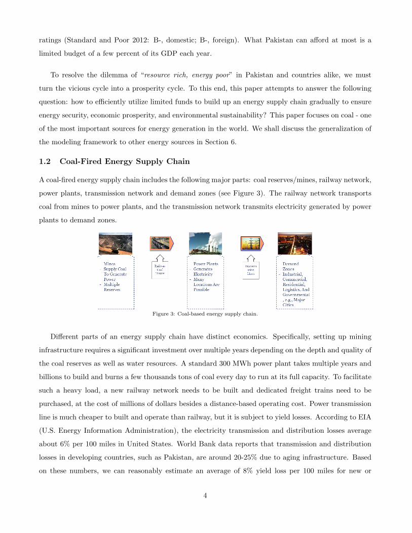
A coal-fired energy supply chain includes the following major parts: coal reserves/mines, railway network,

power plants, transmission network and demand zones (see Figure 3). The railway network transports

coal from mines to power plants, and the transmission network transmits electricity generated by power

plants to demand zones.

Figure 3: Coal-based energy supply chain.

Different parts of an energy supply chain have distinct economics. Specifically, setting up mining

infrastructure requires a significant investment over multiple years depending on the depth and quality of

the coal reserves as well as water resources. A standard 300 MWh power plant takes multiple years and

billions to build and burns a few thousands tons of coal every day to run at its full capacity. To facilitate

such a heavy load, a new railway network needs to be built and dedicated freight trains need to be

purchased, at the cost of millions of dollars besides a distance-based operating cost. Power transmission

line is much cheaper to built and operate than railway, but it is subject to yield losses. According to EIA

(U.S. Energy Information Administration), the electricity transmission and distribution losses average

about 6% per 100 miles in United States. World Bank data reports that transmission and distribution

losses in developing countries, such as Pakistan, are around 20-25% due to aging infrastructure. Based

on these numbers, we can reasonably estimate an average of 8% yield loss per 100 miles for new or

4

upgraded transmission lines in developing countries. Finally, operating a mine or a power plant requires

a variable cost per unit of output.

An energy supply chain has many unique features that distinguish it from the well-studied material

supply chains (i.e., logistics networks).

1. A material supply chain deals with production, distribution and transportation of physical goods.

In contrast, a large part of an energy supply chain deals with energy generation and transmission.

2. Yield loss of power transmission makes an energy supply chain “leaky” while a material supply

chain holds material conservation. Thus a longer distance in material supply chains leads to a

higher transportation cost, but a longer distance in power transmission means that more power

plants need to be built (and more coal to be burnt) to meet the same demand.

3. Coal reserves (the source of energy) are limited and may run out. However, factories and ware-

houses in a material supply chain can run for indefinite times.

4. Energy consumption has a strong impact on GDP, which may affect the budget for energy system

development and in turn energy consumption. This dynamic feedback loop is likely much weaker

in many material supply chains.

To design an energy supply chain, we shall make decisions on reserve selection (which reserves to

mine and when), the number of power plants (PPs) and their locations, rail and power transmission

networks over time. An energy supply chain is an integrated system where decisions on one part may

affect other parts. For example, if PPs are placed near mines but farther away from demand zones,

railway cost for coal transportation will be lower but the yield loss will be higher and so more PPs must

be built. Conversely, if PPs are placed near demand zones, then yield loss will be lower but the railway

cost will be higher. Defining coal-transportation related costs as inbound costs and transmission-yield

induced costs as outbound costs, an effective design of energy supply chains requires a delicate balance of

the trade-off between the inbound and outbound costs. This can be a substantial challenge because (1)

an energy supply chain is a complex network with geographically dispersed demand zones and reserves,

(2) an energy supply system is dynamic in nature due to the limited reserves, fast growing demand, and

the causal relationship between energy consumption, GDP and budget.

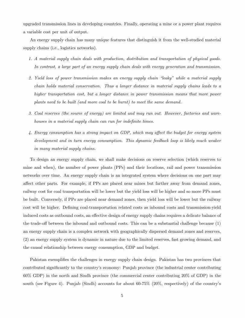
Pakistan exemplifies the challenges in energy supply chain design. Pakistan has two provinces that

contributed significantly to the country’s economy: Punjab province (the industrial center contributing

60% GDP) in the north and Sindh province (the commercial center contributing 20% of GDP) in the

south (see Figure 4). Punjab (Sindh) accounts for about 60-75% (20%, respectively) of the country’s

5

total power consumption. Geographically, major cities of these two provinces scatter across the entire

country with a distance (via railway) between Lahore (the capital city of Punjab) and Karachi (the

capital city of Sindh) of about 800 miles.

Figure 4: Pakistan coal reserves and major GDP provinces. Modified from “Nations Online Project”.

Pakistan has three major coal reserves which account for approximately 98% of the country’s total

coal reserves (see Figure 4): Thar, Sonda/Lakhra and Salt Range. Thar, the largest reserve (essentially

unlimited), is located in the southeast corner of the country far away from all major demand zones. To

set up Thar for mining, a significant amount of infrastructure must be built which will cost at least $6

billion and take 5 years. Salt Range, located in a close proximity to the largest demand zones in Punjab,

is the smallest reserve but only costs $0.5 billion to set up and takes less than 3 years. The medium

reserve at Sonda/Lakhra is near the smaller demand zones in Sindh and would cost $2 billion to set up

and take 3 years.

The geographically dispersed demand zones (large or small) and reserves (expensive or inexpensive)

of Pakistan showcase the challenges in deciding which reserve(s) to mine and where to locate power

plants. Specifically, the fact that the larger reserves (Thar, Sonda/Lakhra) are closer to the smaller

demand zones (Sindh) in the south and the smallest reserve (Salt Range) is closer to the largest demand

zones (Punjab) in the north makes such decisions intriguing and the trade-off between the inbound and

outbound costs hard to balance. Pakistan also has a rapidly growing population and thus faces an

increasing demand of energy at an average of 5-7% annually (Alter and Syed 2011, Iqbal, Nawaz and

6

Anwar 2013).

To save the railway costs and reduce waste from the smaller reserve(s) that may run out, Pakistan

government’s plan is to solve the energy crisis once and for all by mining the distant largest reserve at

Thar and building all power plants nearby. More than 800 miles of transmission lines are planned to

transmit the power from Thar to Punjab province in the north and the rest of the country. Although

this plan is quite intuitive, it raises two concerns: (1) the accumulated yield loss of power transmission

amounts to nearly 50% over the 800-mile distance. Despite savings from railway, one has to double the

number of power plants to get the same output at Punjab. (2) The reserves at Thar are least ready and

require the longest duration and heaviest investment to mine.

While cost is an important factor, time is equally critical in designing energy supply chains. Giving

the fact that Pakistan’s economy is on the verge of collapse, a timely influx of new energy will not only

save the country from bankruptcy but could also jump-start the economy, which in turn allows more

budget to be allocated to the energy sector in the future. Hence, investing in a nearby small reserve that

may run out (like Salt Range) may not be a waste because it is inexpensive and fast, and so can meet

immediate needs. Of course, for such a strategy to work, one must design the energy supply chain in a

way so as to facilitate possible switch to larger reserves in the future.

The complexity and dynamic nature of an energy supply chain in general and the situation of Pakistan

in particular lead us to more specific questions on energy supply chain design: how to design an energy

supply chain to optimally balance the trade-off between inbound and outbound costs? Where to location

PPs (near reserves or demand zones)? How to combine large and small reserves to take advantage of

the economy-energy interaction? And what is the difference that an optimal design can make relative

to intuitive designs such as the plan of Pakistan government?

1.3 Summary of Results

In this paper, we apply supply chain management principles and mathematical programming to the

energy sector and present a new class of mathematical models for designing coal-fired energy supply

chains. For the first time, the model captures the trade-off between inbound and outbound costs in

an integrated energy supply system from coal mining to power generation and to power consumption.

Also for the first time, the model incorporates the dynamic interaction between energy consumption

and economy, and considers limited reserves and the need to switch after they run out. The resulting

mathematic model is a multi-period mixing integer program (MIP) aiming at minimizing energy gaps

among all demand zones by building up an energy supply chain gradually under limited budgets. Deci-

sions are on reserve selection, power plant location, coal transportation and power transmission linkages.

7

Performance metrics are cost per MWh consumed, energy gap, GDP growth, and coal burnt per MWh

consumed (to measure environmental impact).

The mathematical model produces solutions drastically different from the government’s plan. In all

cases (under different budgets, planning horizons, demand growth rates), the optimal solutions utilize

a tiered strategy which first explores the smallest nearby reserve in Punjab (in the north), then the

medium reserve in Sindh (in the south), and finally the largest reserve in Thar (if the planning horizon

is sufficiently long). Power plants are spread out in both north and south near demand zones and are

supplied locally from the small and medium reserves respectively. After the small reserve in the north

runs out, all power plants will be supplied by the medium and large reserves in the south. The optimal

solutions outperform government’s plan significantly by reducing the energy gaps much faster, boosting

the economy much stronger with much less greenhouse gas emissions per MWh consumed.

The rest of this paper is organized as follows: In Section 2, we review the related work in material

supply chain design literature and energy policy/economics literature, and describe in detail our con-

tributions. In Sections 3-4, we present assumptions and justifications, the conceptual model, and the

mathematical model in full detail. In Section 5, we demonstrate the effectiveness of the model and its

solutions through the real-life example of Pakistan in comparison to the government’s plan. Section 6

concludes this paper.

2 Literature Review

This work is related to two broad streams of literature: the design of material supply chains, such

as logistics networks and integrated supply chains; and energy economics and policy. We shall review

related work in both streams and point out the contribution of this work.

2.1 Design of Material Supply Chains

Facility location decisions play a critical role in the strategic design of material supply chains, such

as logistics networks and integrated supply chains of physical goods. A key question answered by the

literature is where to locate plants, warehouses and other facilities in a material supply chain either for

a single period or over multiple periods.

For instance, Geoffrion and Graves (1974) studies the optimal location of intermediate distribu-

tion facilities between plants and customers. A multi-commodity capacitated single-period version of

this problem is formulated as a mixed integer linear program and solved by Benders Decomposition.

Pirkul and Jayaraman (1996) develops a mixed integer programming model for a multi-commodity and

multi-echelon distribution system with the objective of minimizing the transportation and distribution

8

costs as well as the fixed costs for opening and operating the facilities. The model is solved by La-

grangian relaxation and a heuristic. The literature went beyond distribution systems to more integrated

supply chains with both production/logistics and inventory (safety-stock) costs. For instance, Daskin,

Coullard and Shen (2002) considers a distribution-center location model which explicitly incorporates

safety-stock costs and economies of scale in transportation. The model is formulated as a non-linear

integer-programming problem and solved by a Lagrangian relaxation algorithm. Shen, Coullard and

Daskin (2003) studies a joint location-inventory problem where some retailers can serve as distribution

centers to achieve risk pooling effect. The problem is formulated as a set-covering integer-programming

model and solved by column generation algorithms. We refer the reader to Daskin, Snyder and Berger

(2005), and Shen (2007) for reviews of the literature. Shu, Teo and Shen (2005) studies the stochastic

transportation-inventory network design problem involving one supplier and multiple retailers, and show

that by exploiting certain structures, the problem can be solved efficiently. Snyder (2006) surveys the

literature of stochastic and robust facility location models.

Wesolowsky (1973) starts the dynamic facility location literature by studying the single facility lo-

cation problem that permits location changes for a multi-period planning horizon. An algorithm is

developed to optimize the sequence of locations in order to meet changes in cost, volume and location

of destinations. Wesolowsky and Truscott (1975) extends this model to locate multiple facilities among

many possible sites to serve different demand zones. Van Roy and Erlenkotter (1982) solves a capaci-

tated dynamic location problem with opening and closing decisions using a dual-based branch-and-bound

procedure. Love, Morris, and Wesolowsky (1988) provides an early review of this literature.

Hinojosa, Puerto and Fernandez (2000) studies a mixed integer programming model to build facilities

at multiple echelons of a distribution system over time. A dynamic, multiple objective, mixed-integer

programming model is developed by Melachrinoudis and Min (2000) to solve the multi-period relocation

problem. More related work can be found in Canel and Khumawala (1997, 2001) which solve a multi-

period international facilities location problem, Klose and Drexl (2005) which addresses concerns like

which customers should be serviced from which facility (or facilities), Troncoso and Garrido (2005) which

considers specific production and logistics issues in the forest industry, and Dias, Captivo, and Climaco

(2007) which solves a dynamic location problem with opening, closure and reopening of facilities by

primal-dual heuristic approach.

The dynamic facility location literature also considers integrated supply chains with both produc-

tion/logistics and inventory issues. For instance, Gen and Syarif (2005) studies an optimization model

to integrate facility location decisions with inventory management for multiple products and multiple

time periods. Meixell and Gargeya (2005) reviews decision support models for global supply chain de-

9

sign and connects the research literature to practical issues. Altiparmak, Gen, Lin and Paksoy (2006)

proposes a solution procedure based on genetic algorithms to find the set of Pareto-optimal solutions for

multi-objective supply chain network design problem. Fleischmann, Ferber and Henrich (2006) develops

a strategic-planning model for BMW to optimize the allocation of products to global production sites

over a finite planning horizon. We refer the reader to Shapiro (2007) and Simchi-Levi, Kaminsky and

Simchi-Levi (2009) for a thorough review of supply chain modeling and strategies.

The material supply chain design literature provides important modeling and solution methodologies

that can be useful in designing an energy supply chain. However, an energy supply chain is structurally

different from a material supply chain (§1.2) and thus demands new models, performance metrics and

insights. For instance, the unique feature of yield losses in power transmission gives rise to a new trade-

off in energy supply chains (§1.2) that connects the decisions of reserve selection, power plant locations,

and rail/power line linkages. The limited reserves mandate the consideration of mine switching over

time and thus shape the dynamic nature of the model. The interaction between energy consumption

and economy (GDP) not only endogenizes the budget (in contract to exogenous budget often assumed

in the material supply chain literature), but also introduces a dynamic feedback loop that could play

a significant role in system design and configuration. Finally, energy infrastructure development must

account for environmental issues in addition to conventional cost factors.

The energy sector is gaining increasing attention from operations and supply chain management

researchers. We refer the reader to Hu, Kapuscinski and Lovejoy (2011) for a study of auctions in the

wholesale electricity markets, Secomandi and Seppt (2013) for a monograph that provides an integrated

finance and operations perspective, and Fang, Misra, Xue, Yang (2012) for a survey on smart grid - how

to improve efficiency and reliability of existing energy systems. To the best of our knowledge, energy

supply chain design is not studied in the operations and supply chain management literature. In this

paper, we extend the literature of supply chain management from physical goods to energy and energy

resources by developing a new class of location models to capture the unique features of the energy

supply chain.

2.2 Energy Economics and Policy

The energy policy and economics literature studies the specific features of an energy supply chain. Such

studies are either empirical or analytical but often focus on individual parts of an energy supply chain

rather than the supply chain as a whole.

The causal relationship between energy consumption and economy (GDP) is one of most widely

studied relationships in this literature. In the economic theory, energy is considered as an input factor

10

in the production function along with capital and labor. Therefore energy consumption is regarded as

one of the key drivers of economic growth. Solow (1956) is among the first to develop a theory based on

Cobb-Douglas equations to study the influence of energy on the economy. Ever since, the relationship

is empirically estimated and justified by many authors using various data sets. For instance, Oh and

Lee (2004) performs a multivariate analysis on Korea over the period 1970-1999, which suggests a long-

run bidirectional causal relationship between energy and GDP, and a short-run unidirectional causality

running from energy to GDP. Narayan, Narayan and Popp (2010) conducts a multi-country analysis and

confirms that energy consumption has a positive impact on real GDP in countries like Japan, Malaysia,

Pakistan, Sri Lanka, Thailand, and Vietnam. Menegaki (2014) performs a meta-analysis of 51 studies

published in the last two decades, and shows that on average, 1% increase in capital increases the

elasticity of GDP with respect to energy consumption by 0.85%. Multiple studies focus on Pakistan and

justify the causality from electricity consumption to economic growth or industrial output (Shahbaz and

Lean 2012, Shahbaz, Zeshan and Afza 2012, Tang and Shahbaz 2013).

Analytical studies and mathematical modeling in the energy economics and policy literature focus

on three important parts of an energy supply chain: (i) power plant operations and locations, (ii) power

plant fuel transportation, and (iii) electricity transmission.

The literature studies location issues of power plants related to solar, nuclear, wind and thermal

sources. Dutton, Hinman and Millhamet (1974) studies the optimal location of nuclear-power plants

with respect to construction, operating, and transmission costs. The mathematical model was solved by

the simplex method in conjunction with a branch and bound procedure. Barda, Dupuis and Lencioniet

(1990) uses the industrial feasibility standard approach to evaluate the best possible location of power

plants. The paper considers gas transportation by pipelines that differs from coal energy economics.

Rietveld and Ouwersloot (1992) proposes stochastic dominance concepts to rank alternatives among

possible locations for nuclear power plants. An integrated hierarchical approach is presented by Azadeh,

Ghaderi and Maghsoudi (2008) to select the best-possible location for solar power plants with the lowest

costs. This literature also studies power plant operations. For instance, Liu, Huang, Cai, Cheng, Niu,

and An (2009) develops a mathematical programming based optimization model for coal and power

management to improve the efficiency of a coal-based power plant. Godoy, Benz and Scenna (2012)

provides a non-linear programming model to optimize the long-term operations of natural gas combined-

cycle power plants.

The literature also studies the fuel transportation and power transmission issues. For instance,

Mathur, Chand and Tezuka (2003) studies the optimal utilization and transportation of thermal coal

and develops a framework of the general transportation problem based on a linear programming model.

11

Bowen, Canchi, Lalit, Preckel, Sparrow and Irwin (2010) presents a mathematical programming based

multi-period planning model to optimize and expand power transmission system in India with growing

demand for electricity. Paulus and Truby (2011) studies the impact of energy transport decisions on

the global steam coal market by a spatial equilibrium model. Rosnes and Vennemo (2012) builds an

optimization model to estimate the cost of providing electricity to Sub-Saharan Africa over a 10-year

period. These papers consider existing power plants and thus power plant location is not an issue.

All aforementioned analytical papers study individual parts of an energy supply chain rather than the

energy supply chain as a whole. Recently, the potential of such an integrated approach is acknowledged

by Halldorsson and Svanberg (2012), which conceptually explains how supply chain management may

have a great potential in applications to the production, accessibility and use of energy, from the point

of origin to the point of consumption. The paper also points out that “supply chain research has only

to a limited extent explored the nature of energy and energy resources.”

Our work expands the energy economic and policy literature to study an integrated energy supply

chain from coal mining to power consumption based on supply chain management principles and math-

ematical programming models. For the first time, we incorporate the new trade-off between inbound

and outbound costs as well as the dynamic nature of energy supply systems, such as, limited reserves

and energy-GDP interaction, in deciding reserve selection and power plant locations. Applying the

model to the real-life situation of Pakistan, we present novel solutions that significantly outperform the

conventional wisdom in resolving the energy crises and shed new insights on energy supply chain design.

3 Preliminaries

In this section, we make assumptions for a coal-fired energy supply chain and justify them by practices

and standards in the energy sector. We then present a conceptual framework to outline the structure of

the mathematical model.

3.1 Assumptions and Justifications

A coal-fired energy supply chain is a network of typically three echelons: coal reserves, power plants and

demand zones. The coal reserves (upper-most echelon) are mined and coal is transported by trains via

railway to the power plants (middle echelon), where the coal is burnt and the generated electricity is

transmitted by power lines to the demand zones (lowest echelon). Figure 5 provides an overview of the

network structure.

12

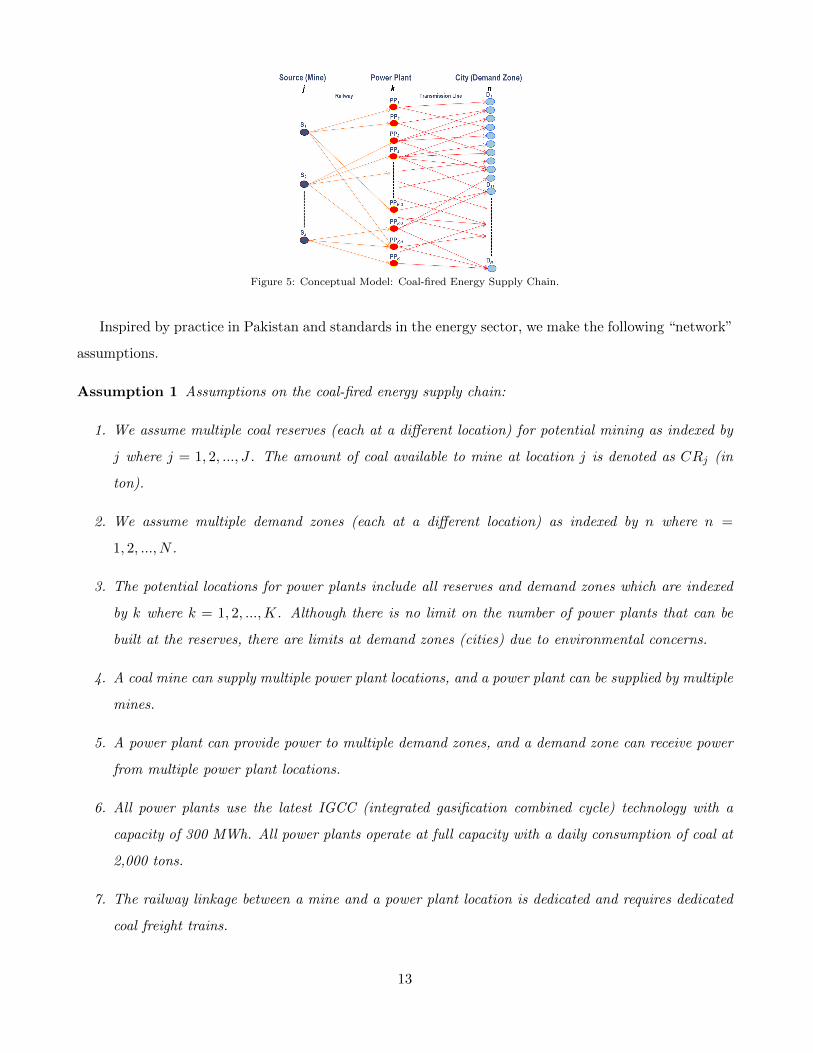
Figure 5: Conceptual Model: Coal-fired Energy Supply Chain.

Inspired by practice in Pakistan and standards in the energy sector, we make the following “network”

assumptions.

Assumption 1 Assumptions on the coal-fired energy supply chain:

1. We assume multiple coal reserves (each at a different location) for potential mining as indexed by

j where j = 1, 2, ..., J . The amount of coal available to mine at location j is denoted as CRj (in

ton).

2. We assume multiple demand zones (each at a different location) as indexed by n where n =

1, 2, ..., N .

3. The potential locations for power plants include all reserves and demand zones which are indexed

by k where k = 1, 2, ...,K. Although there is no limit on the number of power plants that can be

built at the reserves, there are limits at demand zones (cities) due to environmental concerns.

4. A coal mine can supply multiple power plant locations, and a power plant can be supplied by multiple

mines.

5. A power plant can provide power to multiple demand zones, and a demand zone can receive power

from multiple power plant locations.

6. All power plants use the latest IGCC (integrated gasification combined cycle) technology with a

capacity of 300 MWh. All power plants operate at full capacity with a daily consumption of coal at

2,000 tons.

7. The railway linkage between a mine and a power plant location is dedicated and requires dedicated

coal freight trains.

13

8. Building a power plant at a mine requires new transmission; building it at a demand zone requires

upgrading of existing transmission network.

9. The yield loss of transmission lines is 8% for every 100 miles.

The first two assumptions in Assumption 1 are sufficiently general to cover real-life situations in

Pakistan as well as other developing countries around the world. The third assumption is based on

Rafique and Zhao (2011) which provides a thorough case study of the energy crises in Pakistan. This

assumption does not lose generality as we can always include potential locations for power plants as

demand zones. The limitations on the number of power plants are based on pollution and environment

concerns (McMullan, Williams and McCahey 2001, Kavouridisa and Koukouzasb 2008, Chen and Xu

2010). The fourth and fifth assumptions are based on the common industry practice (Rosnes and

Vennemo 2012, Bowen et al. 2010). To justify the sixth assumption, we note that a power plant

with the IGCC technology and 300 MWh capacity is the current standard in practice (Susta 2008).

The seventh assumption can be justified by the heavy load required by power plants. The eighth

assumption comes from the facts that reserves are likely unexplored in many developing countries and

thus have no transmission infrastructure available, whereas in the demand zones, such infrastructure may

be established and thus only an upgrade is needed to deliver a higher volume. The ninth assumption is

justified in Section 1.2.

We shall consider a planning horizon of multiple periods (years), and make the following “regularity”

assumptions:

Assumption 2 Regularity assumptions:

1. The ration of budget allocated to coal-fired energy infrastructure development is RA percent (1%,

2%, 3%, 4%, or 5%) of the real annual GDP (we use real GDP rather than nominal GDP to

eliminate the impact of inflation).

2. The impact of energy consumption on real GDP is country-specific.

3. Once we start construction or updating an energy infrastructure, we must complete the job without

preemption.

4. Power sources other than coal run as BAU (business as usual).

To justify Assumption 2, we first note that developing countries suffering from energy deficiency

can only provide limited funding for energy system development. Using Pakistan as an example, the

budgetary allocation to its energy sector in the last few years ranges from 10% to 15% (Federal Budget

14

Publications 2014-15). However, most of the budget is spent on maintenance and operations of existing

infrastructures. Only a small amount is dedicated to new ventures. Thus any budget allocation of a

higher than 5% of GDP to the new energy projects may be unrealistic. The impact of energy consumption

on the economy (GDP) is observed and justified by the energy economics literature (see Section 2.2 for

details) and confirmed by our regression study of Pakistan (Section 5). We make the third assumption

for convenience because of the unpredictable political circumstances in the next 25 or 50 years. We make

the fourth assumption in order to focus on the energy sources of coal.

3.2 The Conceptual Framework

The mathematical model of an integrated energy supply chain is complex (see Section 4). We shall

present a conceptual framework first to outline its structure and show intuitively how different parts are

connected and interacting.

The objective of the mathematical model is to minimize the total discounted energy gap among

all demand zones over a given planning horizon. Energy gaps are defined as the differences between

projected demand and available supplies. The discounted factors represent a smaller importance for a

more distant year into the future.

From the upper-most echelon to the lowest echelon of an energy supply chain, the decision variables

are: where and when to set up a mine; the location, number and timing of power plant construction;

which mine supplies which power plants; and finally which power plant supplies a demand zone and in

which year.

The constraints can be categorized by echelons and their linkages in the energy supply chain.

1. Mine constraints: Reserves have limited supplies.

2. Railway constraints: Railway and train have capacity limits.

3. Power plant constraints: A limited number of power plants is allowed to built in each potential

location.

4. Network constraints: A power plant’s electricity output can’t exceed the required input of

energy sources (coal) and its capacity.

5. Demand and transmission constraints: The system can’t supply more power (electricity) than

what is needed for each demand zone.

6. Budget constraints: The budget is limited, and energy consumption has an impact on the GDP.

15

While many of these constraints come from capacity limits at various parts of the supply chain, the net-

work constraint connects coal supply with power generation and transmission, and the budget constraint

provides a feedback loop from energy consumption to GDP and to the budget.

The first two categories of constraints can be divided into finer subcategories, specifying availability,

capacity and budget requirement of mining, railway and coal trains. For instance, the availability

constraints of a reserve indicate that it can be setup only once; the capacity constraints honor the limit

of the reserve; and the budget constraints calculate the required budget. The subcategories of capacity

and budget constraints also apply to power plants.

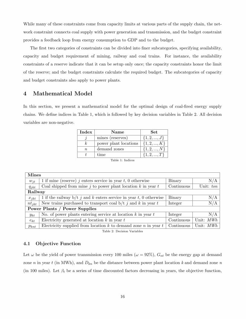
4 Mathematical Model

In this section, we present a mathematical model for the optimal design of coal-fired energy supply

chains. We define indices in Table 1, which is followed by key decision variables in Table 2. All decision

variables are non-negative.

Index Name Set

j mines (reserves) {1, 2, ..., J}k power plant locations {1, 2, ...,K}n demand zones {1, 2, ..., N}t time {1, 2, ..., T}

Table 1: Indices

Mines

wjt 1 if mine (reserve) j enters service in year t, 0 otherwise Binary N/A

qjkt Coal shipped from mine j to power plant location k in year t Continuous Unit: ton

Railway

xjkt 1 if the railway b/t j and k enters service in year t, 0 otherwise Binary N/A

ntjkt New trains purchased to transport coal b/t j and k in year t Integer N/A

Power Plants / Power Supplies

ykt No. of power plants entering service at location k in year t Integer N/A

ekt Electricity generated at location k in year t Continuous Unit: MWh

pknt Electricity supplied from location k to demand zone n in year t Continuous Unit: MWhTable 2: Decision Variables

4.1 Objective Function

Let ω be the yield of power transmission every 100 miles (ω = 92%), Gnt be the energy gap at demand

zone n in year t (in MWh), and Dkn be the distance between power plant location k and demand zone n

(in 100 miles). Let βt be a series of time discounted factors decreasing in years, the objective function,

16

i.e., the total discounted energy gap for all demand zones over a finite planning horizon T is,

T∑t=1

[βt ·N∑n=1

{Gnt − (

K∑k=1

ωDkn · pknt)}] −→Min (1)

The second term in the parenthesis represents the total energy consumed at demand zone n in year t.

4.2 Mine Constraints

The first set of constraints for mines is on their limited reserves, that is, the amount of coal extracted

from mine j up to time t cannot be greater than the total reserve of mine j, CRj (in ton).

K∑k=1

t∑τ=1

qjkτ ≤ CRj ·t∑

τ=1

wjτ for j = 1, . . . , J and t = 1, . . . , T, (2)

where the left-hand-side is the amount of coal extracted from mine j up to year t. Clearly, coal can only

be extracted from mine j if the mine is set up (that is, wjτ = 1 for some τ ≤ t).

The second set of constraints for mines specifies their availability. Because a mine can only be setup

once, thusT∑t=1

wjt ≤ 1 for j = 1, . . . , J. (3)

Because each mine requires time to setup, wjt must satisfy the following initial conditions: wjt = 0, for

t = 1, 2, .., TCMj where TCMj is the reserve/mine specific setup time.

The last set of constraints for mines calculates their capital and operating costs. For mine j, the

setup cost in year t (in $1,000), bCM1jt , can be written as,

bCM1jt = ICMj ·

t+TCMj∑

τ=t+1

wjτ for t = 1, . . . , T − TCMj , (4)

where ICMj is the annual capital investment for setting up mining infrastructure at mine j assuming that

the total investment is evenly distributed over the duration.

Because setting up the mines takes multiple years, it is logical to assume that we cannot start setting

up the mining infrastructure at mine j after the T − TCMj th year as the mine will be ready beyond the

planning horizon and thus cannot contribute to the objective function. Therefore the ending conditions

for mine j are

bCM1jt = ICMj ·

T∑τ=t+1

wjτ for t = T − TCMj + 1, ..., T − 1, (5)

and

bCM1jT = 0. (6)

17

Finally, the operating cost of all mines in year t, bCM2t , is given by

bCM2t = OCCM ·

J∑j=1

K∑k=1

qjkt for t = 1, . . . , T, (7)

where OCCM is the unit operating cost at mines.

4.3 Railway Constraints

We shall only consider railway upgrading in this section. New railway construction uses the same

equations but with different cost and time parameters. The first set of constraints specifies the availability

of the railway. Let Djk be the distance between mine j and power plant location k (in 100 miles) and

M be a large number. Note that xjkt is the indicator on the availability of the railway between j and k

in year t, and ntjkt is an integer variable representing new coal trains purchased on this railway (Table

2), thenT∑t=1

xjkt ≤ 1 where Djk > 0, for j = 1, . . . , J and k = 1, . . . ,K. (8)

Constraint 8 ensures that the railway between mine j and power plant location k is set up only once.

qjkt ≤ CRj ·t∑

τ=1

xjkτ where Djk > 0, for j = 1, . . . , J, k = 1, . . . ,K and t = 1, . . . , T. (9)

Constraint 9 indicates that coal can only be transported if the corresponding railway is set up.

ntjkt ≤M ·t∑

τ=1

xjkτ where Djk > 0, for j = 1, . . . , J, k = 1, . . . ,K and t = 1, . . . , T. (10)

Constraint 10 connects trains to the availability of railway. Because a railway takes multiple years to

setup, we have the following initial conditions: xjkt = 0 for t = 1, 2, ..., TRW where TRW is the railway

setup time.

The second set of constraints is on railway capacity which depends on the frequency and capacity of

trains. Let RTjk be the round trip time between j and k (in hour), then Constraint 11 specifies an upper

limit on the number of trains between j and k.

t∑τ=1

ntjkτ ≤ BF TR ·RTjk for j = 1, . . . , J, k = 1, . . . ,K and t = 1, . . . , T, (11)

where∑t

τ=1 ntjkτ is the total number of trains purchased up to year t to operate on the railway between

j and k, BF TR stands for “buffer of trains”, which is the maximum number of trains allowed to pass

through location k in one hour. Assuming a 10-minute minimum time interval between consecutive

trains, BF TR = 6. We can choose BF TR ·RTjk for the M in constraint 10 for the railway between mine

j and power plant location k.

18

For the railway between j and k, we further define CTRjk = CTR · Fjk to be the annual capacity of

one train (in ton) where CTR is the load of one train, and Fjk (depending on RTjk and can be country

specific) is the maximum frequency (number of round-trips) of a train in one year. Then

qjkt ≤ CTRjk ·t∑

τ=1

ntjkτ where Djk > 0, for j = 1, . . . , J, k = 1, . . . ,K and t = 1, . . . , T.

(12)

Constraint 12 specifies the maximum railway capacity based on train capacity and frequency.

The last set of constraints for railways calculates their capital and operating costs. Let bRW1t (bRW2

t )

be the setup cost (operating cost, respectively) of railways in year t (in $1,000), and bTRt be the cost of

purchasing trains in year t (in $1,000).

bRW1t =

J∑j=1

K∑k=1

(SCRWjkTRW

·t+TRW∑τ=t+1

xjkτ ) for t = 1, . . . , T − TRW , (13)

bRW2t = OCRW ·

J∑j=1

K∑k=1

(Djk · qjkt) for t = 1, . . . , T, (14)

bTRt = ITR ·J∑j=1

K∑k=1

ntjkt for t = 1, . . . , T, (15)

where SCRWjk is the setup cost of railway between j and k, OCRW is the unit operating cost for railway

system, and ITR is the purchasing cost of one train.

Because railway upgrading takes multiple years, so similar to coal mines, we have the following ending

conditions.

bRW1t =

J∑j=1

K∑k=1

(SCRWjkTRW

·T∑

τ=t+1

xjkτ ) for t = T − TRW + 1, ..., T − 1, (16)

bRW1T = 0. (17)

4.4 Network Constraints

This set of constraints ensures that the power plants are adequately supplied from the mines to run at

their full capacity, and the electricity generated at each location, ekt, is transmitted to demand zones.

ekt ≤3

20 · 365·J∑j=1

qjkt for k = 1, . . . ,K and t = 1, . . . , T, (18)

where 320·365 is the conversion rate between coal and power as 2000 tons of coal is needed every day for

a power plant to maintain its full capacity at 300 MWh year around.

ekt ≤ 300 ·t∑

τ=1

ykτ for k = 1, . . . ,K and t = 1, . . . , T. (19)

19

Constraint 19 limits the electricity generated by the power plant capacity.

N∑n=1

pknt ≤ ekt for k = 1, . . . ,K and t = 1, . . . , T. (20)

Constraint 20 ensures that the amount of electricity transmitted is less than electricity generated at each

location.

4.5 Power Plant and Transmission Constraints

The first set of power plant constraints is on their location dependent limitations, UBk, which is the

maximum number of power plants that can be built in location k.

t∑τ=1

ykτ ≤ UBk for k ∈ K and t = 1, . . . , T. (21)

The initial condition for ykt is ykt = 0 for t = 1, 2, ..., TPP where TPP is the setup time for a power

plant.

The second set of constraints for power plants calculates their capital and operating costs. Let IPP

be the annual setup cost of a power plant, OCPP be the annual operating cost per MWh generated

(for a standard 300 MWh power plant), and SCTLk be the location-dependent setup/upgrading cost for

transmission line and grid station. Then the cost of building power plants in year t, bPP1t , and the cost

for building associated grid stations and power plant operations, bPP2t , are

bPP1t = IPP ·

K∑k=1

t+TPP∑τ=t+1

ykτ for t = 1, . . . , T − TPP , (22)

bPP2t =

K∑k=1

{(SCTLk · ykt) + (OCPP · ekt)} for t = 1, . . . , T, (23)

where the operating cost depends on the electricity generated, ekt. Because constructing transmission

lines and grid stations typically take a shorter time than power plants, we assume that such auxiliary

infrastructures are scheduled so as to match the completion time of the corresponding power plant.

Because a power plant takes multiple years to build, similar to coal mines, we have the following

ending conditions.

bPP1t = IPP ·

K∑k=1

T∑τ=t+1

ykτ for t = T − TPP + 1, . . . , T − 1, (24)

bPP1T = 0. (25)

20

4.6 Demand Constraints

Demand constraints ensure that the total amount of electricity supplied at each demand zone is less

than its energy gap.

K∑k=1

(ωDkn · pknt) ≤ Gnt for n = 1, . . . , N and t = 1, . . . , T. (26)

4.7 Budget Constraints

The first set of budget constraints limits the total spending on energy infrastructure development in each

year by the budget.

J∑j=1

bCM1jt + bCM2

t + bRW1t + bRW2

t + bTRt + bPP1t + bPP2

t ≤ gt−1 ·RAt for t = 1, . . . , T, (27)

where RAt is the ration in year t, that is, the % of GDP allocated to the energy sector for these projects;

gt is year t’s real GDP.

The second set of budget constraints connects GDP in year t, gt, to year (t−1)’s energy consumption.

g1 = g0 + Coef ·K∑k=1

N∑n=1

(ωDkn · pkn1), (28)

where g0 is the initial GDP and Coef is the elasticity of GDP with respect to energy consumption, that

is, the slope of the country or economy specific regression model with dependent variable being real GDP

and independent variable being energy (electricity) consumption.

gt = gt−1 + Coef ·K∑k=1

N∑n=1

{ωDkn · (pknt − pknt−1)} for t = 2, . . . , T. (29)

Specifically, GDP growth in year t depends on how much more electricity is consumed in this year than

the previous year.

5 Solution and Impact

In this section, we apply the mathematical model (developed in Section 4) to Pakistan and demonstrate

its potential impact. Section 5.1 presents the real-life situations of Pakistan, and Section 5.2 provides

solutions and insights.

5.1 The Case of Pakistan

A map of Pakistan coal reserves and major demand zones is shown in Figure 6.

21

Figure 6: Pakistan map with major coal reserves and demand zones. Modified from “Pakistan Railways NetworkMap” by Adnanrail Licensed under Creative Commons Attribution-Share Alike 3.0 via Wikimedia Commons.

A thorough case study of Pakistan’s energy crises by Rafique and Zhao (2011) provides the following

observations.

Observation 1 Observations on the coal-fired energy supply chain of Pakistan:

1. Three largest coal reserves (Figure 6): Thar, Sonda/Lakhra and Salt Range, account for 98% of

Pakistan’s total coal reserves, J = 3. The reserves that are of sufficient quality for power generation

are listed in Table 3. As we can see, Thar and Sonda/Lakhra reserves have ample reserves to meet

demand in a planning horizon of 25 or 50 years but Salt Range does not.

2. There are 19 demand zones that account for 90% of the country’s total energy consumption (Figure

6), N = 19. 14 of them are major energy-consumption cities and 5 of them are smaller cities but

ideal locations for power plants. Demand for energy is estimated to grow at a rate of 5-7% annually

(Section 1.2).

3. The potential locations for power plants include all reserves and demand zones, thus there are 22

locations (K = 22).

4. There is no limit on the number of power plants that can be built at the three coal reserves, that is,

UBj = +∞ for j ∈ KR where KR is the set of power plant locations at coal reserves. For demand

zones, at most ten power plants (UBj = 10) can be built in each of the five smaller cities j ∈ KS;

at most five power plants (UBj = 5) can be built in the other bigger cities j ∈ KB.

22

We consider a planning horizon of either 25 years or 50 years (T = 25 or 50).

Name Province Reserves (Million Tons) CRj/106 Years of 10,000 MWh generated

Salt Range Punjab 213 9

Sonda and Lakhra Sindh 8,440 350

Thar Sindh 175,000 7,251

Table 3: Pakistan Coal Reserves. Source: Rafique and Zhao (2011).

Table 4 specifies the model parameters for Pakistan.

Mines:

TCM1 Setup time for Thar reserve 5 years

TCM2 Setup time for Sonda/Lakhra reserve 3 years

TCM3 Setup time for Salt Range reserve 3 years

ICM1 Annual investment for mine setup at Thar 6, 000, 000/5 in $1,000

ICM2 Annual investment for mine setup at Sonda/Lakhra 2, 000, 000/3 in $1,000

ICM3 Annual investment for mine setup at Salt Range 500, 000/3 in $1,000

OCCM Unit operating cost at mines 5.33× 10−3 per ton in $1,000

Railway / Train:

TRW Setup time for railways 3 (5) years for upgrading (for new)

RTjk Round trip time between j and k in hour

CTR Load of one train 15,000, in ton

Fjk Maximum annual frequency of a train on the railway between j and k N/A

SCRWjk Setup cost of the railway between j and k in $1,000

OCRW Unit operating cost for railway coal transport 0.04× 10−3 per ton per mile, in $1,000

ITR Purchasing cost of one train 50,000, in $1,000

Power Plant / Transmission Line:

TPP Setup time for a standard 300 MWh power plant 3 years

IPP Annual setup cost of a standard 300 MWh power plant 1,000,000/3 in $1,000

OCPP Annual operating cost of a standard 300 MWh power plant 2% of the total setup cost

SCTLk Setup cost of transmission and grid station at location k in $1,000for a new power plant

Demand / Distances

Gnt Energy gap at demand zone n in year t in MWh

Djk Distance between j and k in 100 miles

Dkn Distance between k and n in 100 miles

Table 4: Parameters for Pakistan. Sources: Rafique and Zhao (2011).

Note that the mine setup costs, ICMj , include water supply related costs. The matrices of Djk and

Dkn are determined by the geology and transportation network of Pakistan. RTjk = 2Djk/0.5+LT+UT

where 0.5 refers to the average train speed of 50 miles/hour, and LT (UT ) refers to loading (unloading,

respectively) time. Fjk = 24/RTjk · 365 where the numbers 24 and 365 refer to 24 hours a day and 365

days a year respectively. Gnt depends on the demand of the starting year and the projected growth rate.

The cost matrix of railway, SCRWjk , is calculated by the distance matrix Djk and a setup cost of $0.73

million/mile for upgrading (or $13 million/mile for new construction) (Ministry of Pakistan Railway).

The setup cost of transmission and grid station for a new power plant, SCTLk , is calculated by the

distance from location k to the nearest grid station and a transmission line cost of $1.8 million/mile for

new (or $0.6 million/mile for upgrading) as well as a local grid station cost of $33,000/ MWh (American

Electric Power, Transmission Facts).

23

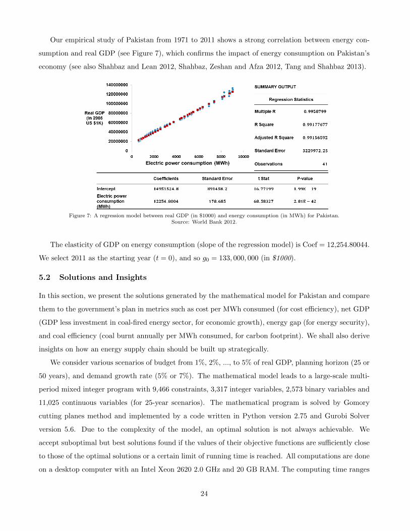
Our empirical study of Pakistan from 1971 to 2011 shows a strong correlation between energy con-

sumption and real GDP (see Figure 7), which confirms the impact of energy consumption on Pakistan’s

economy (see also Shahbaz and Lean 2012, Shahbaz, Zeshan and Afza 2012, Tang and Shahbaz 2013).

Figure 7: A regression model between real GDP (in $1000) and energy consumption (in MWh) for Pakistan.Source: World Bank 2012.

The elasticity of GDP on energy consumption (slope of the regression model) is Coef = 12,254.80044.

We select 2011 as the starting year (t = 0), and so g0 = 133, 000, 000 (in $1000).

5.2 Solutions and Insights

In this section, we present the solutions generated by the mathematical model for Pakistan and compare

them to the government’s plan in metrics such as cost per MWh consumed (for cost efficiency), net GDP

(GDP less investment in coal-fired energy sector, for economic growth), energy gap (for energy security),

and coal efficiency (coal burnt annually per MWh consumed, for carbon footprint). We shall also derive

insights on how an energy supply chain should be built up strategically.

We consider various scenarios of budget from 1%, 2%, ..., to 5% of real GDP, planning horizon (25 or

50 years), and demand growth rate (5% or 7%). The mathematical model leads to a large-scale multi-

period mixed integer program with 9,466 constraints, 3,317 integer variables, 2,573 binary variables and

11,025 continuous variables (for 25-year scenarios). The mathematical program is solved by Gomory

cutting planes method and implemented by a code written in Python version 2.75 and Gurobi Solver

version 5.6. Due to the complexity of the model, an optimal solution is not always achievable. We

accept suboptimal but best solutions found if the values of their objective functions are sufficiently close

to those of the optimal solutions or a certain limit of running time is reached. All computations are done

on a desktop computer with an Intel Xeon 2620 2.0 GHz and 20 GB RAM. The computing time ranges

24

from 4 minutes to 1,344 minutes (see Appendix for details).

The mathematical model provides intriguing solutions, which are drastically different from the gov-

ernment’s plan. Recall that the government’s plan explores only the largest reserve at Thar and builds

all power plants at that location. For comparison, let’s consider a representative scenario with 5% de-

mand growth, a budget of 3% of GDP and a planning horizon of 25 years (see Figure 8). The optimal

solution first mines the smallest reserve (Salt Range in the north) near the largest demand zones (the

industrial hub in Punjab) that requires much less time and capital to setup than other reserves. The

medium reserve at Sonda/Lakhra (in the south) near the commercial hub in Sindh is next explored, but

the largest reserve at Thar (in the southeast corner) is not setup for mining throughout the planning

horizon in this scenario. Power plants are first built at the largest demand zones in Punjab and supplied

locally by the Salt Range mine so as to minimize the yield loss at an affordable coal transportation cost.

After the medium reserve at Sonda/Lakhra is setup, power plants are then built at demand zones in

Sindh and supplied locally by the Sonda/Lakhra mine. When the Salt Range mine runs out (it depletes

in about 20 years in this scenario), the power plants in Punjab shall switch supply from Salt Range to

Sonda/Lakhra in Sindh. Power plants may be built at coal reserves after nearby demand zones run out

of space.

Figure 8: The optimal solution on reserve selection and power plant locations for the scenario with 5% demandgrowth, a budget of 3% GDP and a 25-year planning horizon. Circles - coal reserves; empty circles - reservesthat run out; collate shapes - power plants (the box below indicates the number of power plants in service).

25

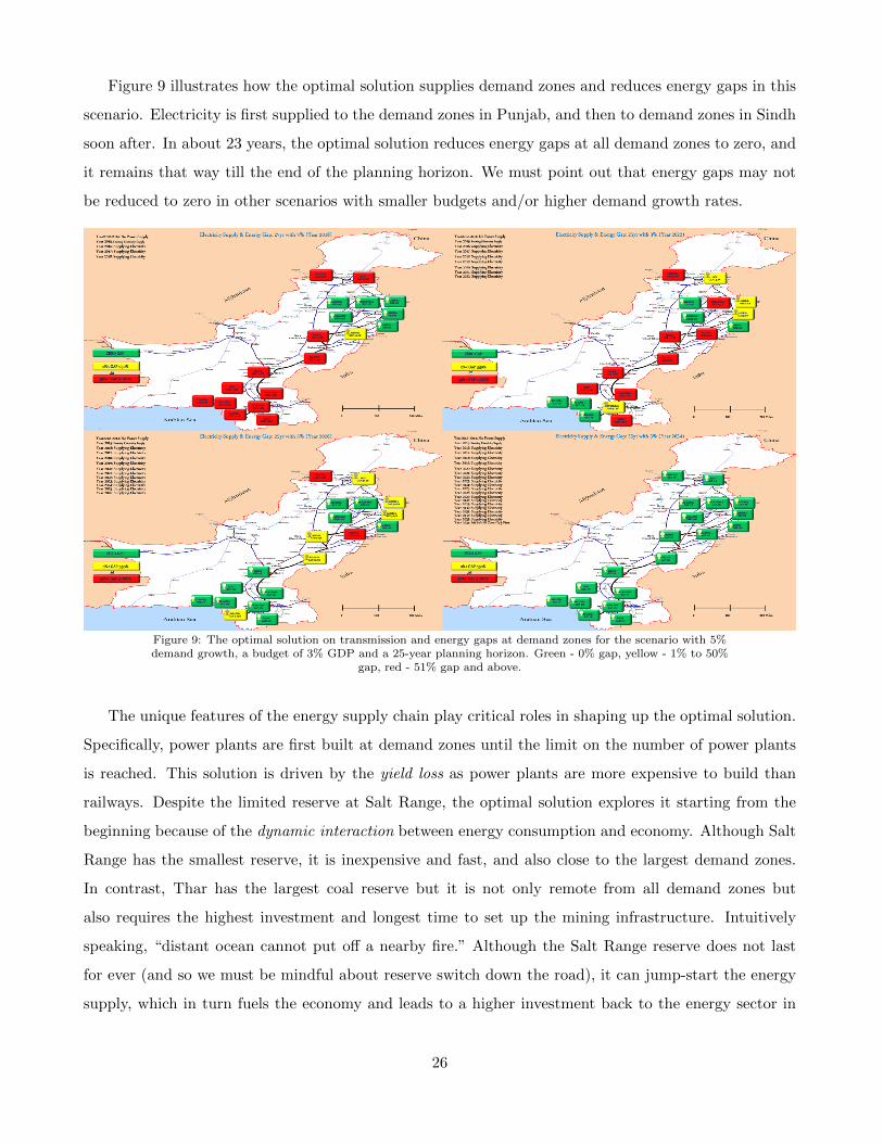
Figure 9 illustrates how the optimal solution supplies demand zones and reduces energy gaps in this

scenario. Electricity is first supplied to the demand zones in Punjab, and then to demand zones in Sindh

soon after. In about 23 years, the optimal solution reduces energy gaps at all demand zones to zero, and

it remains that way till the end of the planning horizon. We must point out that energy gaps may not

be reduced to zero in other scenarios with smaller budgets and/or higher demand growth rates.

Figure 9: The optimal solution on transmission and energy gaps at demand zones for the scenario with 5%demand growth, a budget of 3% GDP and a 25-year planning horizon. Green - 0% gap, yellow - 1% to 50%

gap, red - 51% gap and above.

The unique features of the energy supply chain play critical roles in shaping up the optimal solution.

Specifically, power plants are first built at demand zones until the limit on the number of power plants

is reached. This solution is driven by the yield loss as power plants are more expensive to build than

railways. Despite the limited reserve at Salt Range, the optimal solution explores it starting from the

beginning because of the dynamic interaction between energy consumption and economy. Although Salt

Range has the smallest reserve, it is inexpensive and fast, and also close to the largest demand zones.

In contrast, Thar has the largest coal reserve but it is not only remote from all demand zones but

also requires the highest investment and longest time to set up the mining infrastructure. Intuitively

speaking, “distant ocean cannot put off a nearby fire.” Although the Salt Range reserve does not last

for ever (and so we must be mindful about reserve switch down the road), it can jump-start the energy

supply, which in turn fuels the economy and leads to a higher investment back to the energy sector in

26

the future (to explore, for instance, the Thar reserve). Doing so can help turning the vicious energy-

economic cycle into a prosperity cycle. Thus the capital spent to set up Salt Range is not a waste but a

worthy investment.

To quantify the impact of the optimal solution, we compare it to the government’s plan on four

metrics (Figure 10): cost efficiency, i.e., cumulative cost over cumulative MWh consumed (a), net GDP

(b), country-wide energy gap (c) and coal efficiency (d).

Figure 10: Optimal solution vs. Government’s plan. The x-axis is on time (in year). 5% demand growth, 3%ration and 25-year planning horizon.

As we can see, the optimal solution significantly outperforms the government’s plan by spending

much less for each MWh consumed (Figure 10a), boosting the economy much stronger (Figure 10b),

reducing the energy gaps much faster (Figure 10c) with less coal burnt per MWh consumed (Figure

10d). The optimal solution delivers much more electricity to the demand zones with a higher coal

efficiency than the government’s plan, and thus it is more sustainable in the sense of economy and

environment. Specifically, the optimal solution can reduce the energy gap down to zero in about 23

27

years while the government’s plan maintains an approximately 36.92% energy deficiency towards the

end of planning horizon. Consequently, the optimal solution will generate a net GDP in the 25th year of

$639 billion, as compared to $406 billion of the government’s plan. Finally, for every MWh consumed,

the government’s plan requires 2,898-3,496 tons of coal annually but the optimal plan only requires about

2,439-2,702 tons.

In other budgetary scenarios of 5% demand growth and 25-year planning horizon, the solutions stay

qualitatively the same. The most notable difference between the scenarios with less than 3% rations and

the scenario with 3% ration is that in the former, we do not have enough money to reduce the energy

gap to zero. For instance, in the scenario of 1% ration, the energy gap will rise in both the optimal

solution and the government’s plan to 65% and 70% respectively in 25th year. Interestingly, the optimal

solution still significantly outperforms the government’s plan on the net GDP ($228 billion vs. $195

billion) and coal efficiency (2,437-2,461 tons vs. 2,744-2,876 tons annually per MWh consumed). In the

scenario of a 2% ration, the energy gap will rise in the government’s plan to about 53% in the 25th year

but decrease in the optimal solution to around 36%. Consequently, the optimal solution outperforms

the government’s plan on the net GDP ($412 billion vs. $305 billion) in the 25th year. In scenarios

with more than 3% rations, the optimal solution will reduce energy gaps to zero much sooner than the

government’s plan with higher net GDP and coal efficiency. Thus, our model can be used to justify the

budget required to bring down the energy gap to zero in targeted years. Increasing the planning horizon

from 25 years to 50 years does not change the trend of the energy gap, net GDP and coal efficiency in all

scenarios but widens the differences in the net GDPs (especially in scenarios with less than 3% rations).

In addition, the optimal solution may explore Thar after the 25th year mark.

The improvement on GDP made by the optimal solution relative to the government’s plan depends

on the budget. Figure 11 shows the average GDP per year (in $ million) under the government’s plan

and the optimal solution for various budgetary conditions (% of GDP). The figure shows that although

the optimal solution always outperforms the government’s plan, it makes the greatest difference on

the average GDP when the budget is neither too tight nor too generous. Intuitively, if the budget is

very tight, it allows little flexibility for the optimal solution to improve; if the budget is very generous,

cost efficiency as achieved by the optimal solution becomes relatively unimportant because funding is

abundant.

28

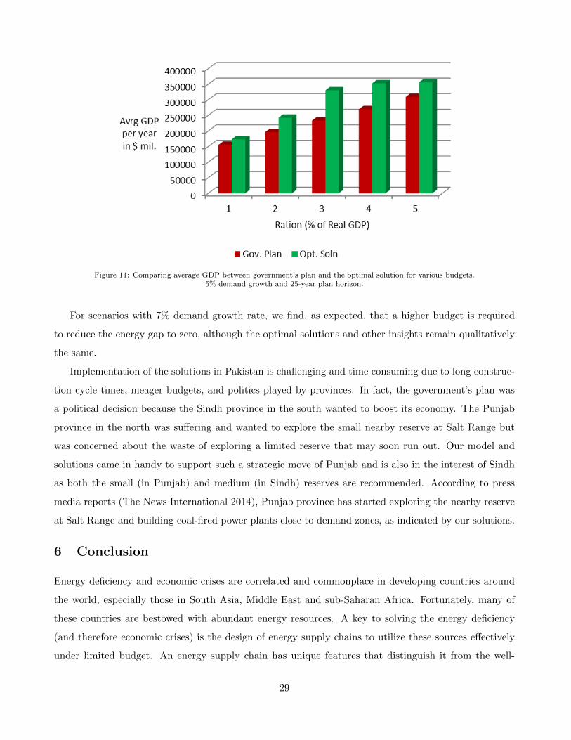
Figure 11: Comparing average GDP between government’s plan and the optimal solution for various budgets.5% demand growth and 25-year plan horizon.

For scenarios with 7% demand growth rate, we find, as expected, that a higher budget is required

to reduce the energy gap to zero, although the optimal solutions and other insights remain qualitatively

the same.

Implementation of the solutions in Pakistan is challenging and time consuming due to long construc-

tion cycle times, meager budgets, and politics played by provinces. In fact, the government’s plan was

a political decision because the Sindh province in the south wanted to boost its economy. The Punjab

province in the north was suffering and wanted to explore the small nearby reserve at Salt Range but

was concerned about the waste of exploring a limited reserve that may soon run out. Our model and

solutions came in handy to support such a strategic move of Punjab and is also in the interest of Sindh

as both the small (in Punjab) and medium (in Sindh) reserves are recommended. According to press

media reports (The News International 2014), Punjab province has started exploring the nearby reserve

at Salt Range and building coal-fired power plants close to demand zones, as indicated by our solutions.

6 Conclusion

Energy deficiency and economic crises are correlated and commonplace in developing countries around

the world, especially those in South Asia, Middle East and sub-Saharan Africa. Fortunately, many of

these countries are bestowed with abundant energy resources. A key to solving the energy deficiency

(and therefore economic crises) is the design of energy supply chains to utilize these sources effectively

under limited budget. An energy supply chain has unique features that distinguish it from the well-

29

studied material supply chains, such as, yield loss of power transmission, limited reserves, and a strong

interaction between energy consumption and GDP. In this paper, we construct a novel mathematic model

to capture these features of energy supply chains. Applying to the real life situation of Pakistan, we

demonstrate the potential of the model in breaking the vicious energy-economy cycle and in improving

energy security, economic prosperity and environmental sustainability.

We can extend the mathematical model developed for coal to address similar issues with other energy

resources such as oil, gas and hydro, etc. Different energy sources have difference economics in certain

part(s) of the energy supply chain. For instance, gas can be transported either by pipelines or in the form

of liquefied natural gas (LNG), which have distinct cost structures from coal; oil-based energy supply

chains have similar features as gas-based ones except for an additional echelon of oil refineries. Hydro is

one of the cleanest and most efficient energy sources but the location of hydro dams depends not only

on energy needs but also irrigation in the agriculture sector and concerns of flood. We expect that the

mathematical model, after proper customization to each energy source, may make significant differences

in developing countries, and help them to resolve the dilemma of “resource rich, energy poor”.

Although this study demonstrates the effectiveness of our model in addressing the energy gaps

through coal-fired energy supply chain, in real world, a combination of coal and other energy options

such as nuclear and renewable resources (hydro, solar and wind) is desirable for achieving a more bal-

anced energy mix. In fact, an over-reliance on electricity generated through coal can pose a serious

challenge on security, maintenance and environmental issues (Pakistan is currently free of this concern

as the contribution of coal to the energy mix is only 0.2%). Ultimately, it is an energy-mix issue: how to

optimally balance the energy mix from a portfolio of energy resources? How to optimally utilize different

resources of energy under a limited budget? These questions clearly take the research to the next-level of

complexity and we plan to answer them in future studies. We also plan to characterize the mathematical

properties of energy supply chains to enable more efficient solution algorithms. Finally, this research

may serve as a starting point at the interfaces between supply chain management and energy economics

to aid policy makers in the energy sector.

Appendix

Table 5 summarizes the CPU times and optimality gaps for the scenarios discussed in Section 5.2.

30

Demand Planning Ration Optimality Running Type and numberGrowth Horizon (% of GDP) Gap (%) Time of Variable

1% 4.9937% 216.11 sec Variable Type:2% 7.5839% 3,315.00 sec 11,025 continuous, 3,317

25 years 3% 8.6058% 29,678.00 sec integer (2,573 binary)4% 0.8686% 4,288.95 sec

5% 5% 9.2671% 667.37 sec1% 8.5173% 5,718.00 sec2% 11.8825% 26,218.00 sec Variable Type:

50 years 3% 20.9940% 80,633.03 sec 23,711 continuous, 7,0934% 7.8265% 19,247.00 sec integer (5,497 binary)5% 4.4076% 10,285.73 sec

Table 5: CPU Time and Optimality Gaps

References

[1] Alter, N. and Syed, S. H. (2011). An empirical analysis of electricity demand in Pakistan.International Journal of Energy Economics and Policy, 1(4):116–139.

[2] Altiparmak, F., Gen, M., Lin, L., and Paksoy, T. (2006). A genetic algorithm approach formulti-objective optimization of supply chain networks. Computers & Industrial Engineering,51(1):196–215.

[3] American Electric Power, Transmission Facts.<http://www.aep.com/about/transmission/docs/transmission-facts.pdf>. Accessed onAug 12, 2012.

[4] Azadeh, A., Ghaderi, S., and Maghsoudi, A. (2008). Location optimization of solar plants by anintegrated hierarchical DEA PCA approach. Energy Policy, 36(10):3993–4004.

[5] Barda, O. H., Dupuis, J., and Lencioni, P. (1990). Multicriteria location of thermal power plants.European Journal of Operational Research, 45(2):332–346.

[6] Bowen, B. H., Canchi, D., Lalit, V. A., Preckel, P. V., Sparrow, F., and Irwin, M. W. (2010).Planning India’s long-term energy shipment infrastructures for electricity and coal. Energy Policy,38(1):432–444.

[7] Canel, C. and Khumawala, B. M. (1997). Multi-period international facilities location: Analgorithm and application. International Journal of Production Research, 35(7):1891–1910.

[8] Canel, C. and Khumawala, B. M. (2001). International facilities location: a heuristic procedure forthe dynamic uncapacitated problem. International Journal of Production Research,39(17):3975–4000.

[9] Chen, W. and Xu, R. (2010). Clean coal technology development in china. Energy Policy,38(5):2123–2130.

[10] Daskin, M. S., Coullard, C. R., and Shen, Z.-J. M. (2002). An inventory-location model:Formulation, solution algorithm and computational results. Annals of Operations Research,110(1-4):83–106.

[11] Daskin, M. S., Snyder, L. V., and Berger, R. T. (2005). Facility location in supply chain design. InLogistics systems: Design and optimization, pages 39–65. Springer.

[12] Dias, J., Eugenia Captivo, M., and Clımaco, J. (2007). Efficient primal-dual heuristic for adynamic location problem. Computers & operations research, 34(6):1800–1823.

[13] Dutton, R., Hinman, G., and Millham, C. (1974). The optimal location of nuclear-power facilitiesin the pacific northwest. Operations Research, 22(3):478–487.

31

[14] Fang, X., Misra, S., Xue, G., Yang, D. (2012). Smart grid - the new and improved power grid: asurvey. IEEE Communications Surveys and Tutorials, 14(4): 944–980.

[15] Federal Budget Publications 2014-15 (Ministry of Finance, Government of Pakistan, 2014).Available at <http://www.finance.gov.pk/fb_2014_15.html>. Retrieved on Oct 14, 2014.

[16] Fleischmann, B., Ferber, S., and Henrich, P. (2006). Strategic planning of BMW’s globalproduction network. Interfaces, 36(3):194–208.

[17] Geoffrion, A. M. and Graves, G. W. (1974). Multicommodity distribution system design bybenders decomposition. Management science, 20(5):822–844.

[18] Gen, M. and Syarif, A. (2005). Hybrid genetic algorithm for multi-time periodproduction/distribution planning. Computers & Industrial Engineering, 48(4):799–809.

[19] Godoy, E., Benz, S., and Scenna, N. (2012). Optimal economic strategy for the multiperiod designand long-term operation of natural gas combined cycle power plants. Applied Thermal Engineering.

[20] Halldorsson, A. and Svanberg, M. (2012). Energy resources: Trajectories for supply chainmanagement. Supply Chain Management: An International Journal, 18(1):5–5.

[21] Hinojosa, Y., Puerto, J., and Fernandez, F. R. (2000). A multiperiod two-echelon multicommoditycapacitated plant location problem. European Journal of Operational Research, 123(2):271–291.

[22] Hu, S., Kapuscinski, R., Lovejoy, W. (2011). Price dispersion and electricity auctions: thestrategic foundation and implication to market design. Working Paper, Ross School of Business,University of Michigan.

[23] IEA (International Energy Agency, 2011). World energy outlook. 2011. OECD Publications, Paris.

[24] Iqbal, N., Nawaz, S., and Anwar, S. (2013). Electricity demand in Pakistan: A nonlinearestimation. Technical report, Mimeo Pakistan Institute of Development Economics.

[25] Kavouridis, K. and Koukouzas, N. (2008). Coal and sustainable energy supply challenges andbarriers. Energy Policy, 36(2):693–703.

[26] Kiernan, P. (2014). Africa: Resource rich, energy poor. Available at <http://geafricaascending.economist.com/2014/07/31/africa-resource-rich-energy-poor/>.Retrieved on December 31, 2014.

[27] Klose, A. and Drexl, A. (2005). Facility location models for distribution system design. EuropeanJournal of Operational Research, 162(1):4–29.

[28] Kugelman, M. (2013). Pakistan’s energy crisis: From conundrum to catastrophe? Available at<http://www.nbr.org/downloads/pdfs/eta/Kugelman_commentary_03132013.pdf>. Retrievedon Jan 27, 2014.

[29] Liu, Y., Huang, G., Cai, Y., Cheng, G., Niu, Y., and An, K. (2009). Development of an inexactoptimization model for coupled coal and power management in north china. Energy Policy,37(11):4345–4363.

[30] Love, R. F., Morris, J. J., and Wesolowsky, G. O. (1988). Facilities location, volume 90.North-Holland Amsterdam.

[31] Malik, A. (2008). How Pakistan is coping with the challenge of high oil prices. The PakistanDevelopment Review, 46(4):551–575.

[32] Malik, A. (2010). Oil prices and economic activity in Pakistan. South Asia Economic Journal,11(2):223–244.

32

[33] Mathur, R., Chand, S., and Tezuka, T. (2003). Optimal use of coal for power generation in India.Energy policy, 31(4):319–331.

[34] McMullan, J., Williams, B., and McCahey, S. (2001). Strategic considerations for clean coal R&D.Energy Policy, 29(6):441–452.

[35] Meixell, M. J. and Gargeya, V. B. (2005). Global supply chain design: A literature review andcritique. Transportation Research Part E: Logistics and Transportation Review, 41(6):531–550.

[36] Melachrinoudis, E. and Min, H. (2000). The dynamic relocation and phase-out of a hybrid,two-echelon plant/warehousing facility: A multiple objective approach. European Journal ofOperational Research, 123(1):1–15.

[37] Menegaki, A. N. (2014). On energy consumption and GDP studies; a meta-analysis of the last twodecades. Renewable and Sustainable Energy Reviews, 29:31–36.

[38] Ministry of Pakistan Railway. <http://www.railways.gov.pk>. Accessed on Feb 08, 2011.

[39] Narayan, P. K., Narayan, S., and Popp, S. (2010). A note on the long-run elasticities from theenergy consumption–GDP relationship. Applied Energy, 87(3):1054–1057.

[40] NEPRA (National Electric Power Regulatory Authority, 2011). State of industry report 2011.Available at <http://nepra.org.pk/industryreports.htm>. Retrieved on Feb 01, 2014.

[41] Oh, W. and Lee, K. (2004). Causal relationship between energy consumption and GDP revisited:the case of Korea 1970–1999. Energy economics, 26(1):51–59.

[42] Pakistan Railway Network Map by Adnanrail (2012). Licensed under Creative CommonsAttribution-Share Alike 3.0 via Wikimedia Commons. Available at<http://commons.wikimedia.org/wiki/File:Pakistan_Railways_Map.png>. Accessed on Dec05, 2013.

[43] Paulus, M. and Truby, J. (2011). Coal lumps vs. electrons: How do Chinese bulk energy transportdecisions affect the global steam coal market? Energy Economics, 33(6):1127–1137.

[44] Pirkul, H. and Jayaraman, V. (1996). Production, transportation, and distribution planning in amulti-commodity tri-echelon system. Transportation Science, 30(4):291–302.

[45] Rafique, R. and Zhao, Y. (2011). Pakistan Energy Crisis - Breaking the Vicious Cycle. CaseStudy, Rutgers Business School - Newark and New Brunswick.

[46] Rietveld, P. and Ouwersloot, H. (1992). Ordinal data in multicriteria decision making, a stochasticdominance approach to siting nuclear power plants. European Journal of Operational Research,56(2):249–262.

[47] Rosnes, O. and Vennemo, H. (2012). The cost of providing electricity to Africa. EnergyEconomics, 34(5):1318–1328.

[48] Santana, R. (2013). Pakistan’s power shortage problem is country’s biggest threat. Available at<http://www.huffingtonpost.com/2013/06/15/pakistan-power-shortage_n_3447599.html>.Retrieved on Feb 01, 2014.

[49] Secomandi, N., and Seppi, D. J. (2013). Real options and merchant operations of energy and othercommodities. forthcoming in Foundations and Trends in Technology, Information and OperationsManagement.

[50] Shahbaz, M., Zeshan, M., and Afza, T. (2012). Is energy consumption effective to spur economicgrowth in Pakistan? New evidence from bounds test to level relationships and granger causalitytests. Economic Modelling, 29 (6):2310–2319.

33

[51] Shapiro, J. F. (2007). Modeling the supply chain, volume 2. Cengage Learning.

[52] Shen, Z.-J. M., Coullard, C., and Daskin, M. S. (2003). A joint location-inventory model.Transportation Science, 37(1):40–55.

[53] Shen, Z. (2007). Integrated supply chain design models: A survey and future research directions.Journal of Industrial and Management Optimization, 3(1):1.

[54] Shu, J., Teo, C. P., Shen, Z. J. (2005). Stochastic Transportation-inventory Network DesignProblem. Operations Research, 53: 48–60.

[55] Simchi-Levi, D. (2009). Designing and managing the supply chain concepts, strategies, and casestudies. Tata McGraw-Hill Education.

[56] Snyder, L. V. (2006). Facility location under uncertainty: A review. IIE Transactions,38(7):547–564.

[57] Solow, R. M. (1956). A contribution to the theory of economic growth. The quarterly journal ofeconomics, 70(1):65–94.

[58] Susta, M. R. (2008). Development in Supercritical Steam Tech. Powergen Asia 2008, KualaLumpur, Oct. 2008.

[59] Tang, C. F. and Shahbaz, M. (2013). Sectoral analysis of the causal relationship betweenelectricity consumption and real output in pakistan. Energy Policy, 60:885–891.

[60] The Nations Online Project (1998-2011). Let’s care for this planet. Copyright 1998-2011.<http://www.nationsonline.org/oneworld/map/pakistan_map.htm>. Accessed on Dec 31,2014.

[61] The News International (2014). CM welcomes Chinese investment in coal mining. Tuesday, March18. Extracted from <http://www.thenews.com.pk/> on March 20, 2014.

[62] Troncoso, J. J. and Garrido, R. A. (2005). Forestry production and logistics planning: an analysisusing mixed-integer programming. Forest Policy and Economics, 7(4):625–633.

[63] Van Roy, T. J. and Erlenkotter, D. (1982). A dual-based procedure for dynamic facility location.Management Science, 28(10):1091–1105.

[64] Wesolowsky, G. O. (1973). Dynamic facility location. Management Science, 19(11):1241–1248.

[65] Wesolowsky, G. O. and Truscott, W. G. (1975). The multiperiod location-allocation problem withrelocation of facilities. Management Science, 22(1):57–65.

[66] World Bank. (2012). The World Bank Data, Pakistan, (2012).<http://data.worldbank.org/country/pakistan>. Accessed on Sep 27, 2013.

34