energy system analysis - diva portal
TRANSCRIPT

Thesis number 2016-13-09
ENERGY SYSTEM
ANALYSIS
Ranjith Soundararajan

ii
ENERGY SYSTEM ANALYSIS
Ranjith Soundararajan, [email protected]
Master thesis
Subject Category: Technology
Examiner: Professor Tobias Richards
Supervisor, name: Professor Tobias Richards
Supervisor address: University of Borås
School of Engineering
SE-501 90 BORÅS
Telephone +46 033 435 4640
SE-50190 BORAS
Date: 1-10-2016
Keywords: Pinch technology, heat exchanger network, MATLAB, linear
programming, genetic algorithm

iii
Abstract
In the past decades, many synthesis of heat exchanger network is proposed to minimize the
annual cost. The purpose of this thesis is to use a model to optimize the heat exchanger
network for process industry and to estimate the minimum cost required for the heat
exchanger network without compromising the energy demand by each stream as much as
possible with the help of MATLAB programming software. Here, the optimization is done
without considering stream splitting and stream combining. The first phase involves with
deriving a simple heat exchanger network consisting of four streams i.e... Two hot streams
and two cold streams required for the heat exchanger using the traditional Pinch Analysis
method. The second phase of this work deals with randomly placing the heat exchanger
network between the hot and cold streams and calculating the minimum cost of the heat
exchanger network using genetic coding which is nothing but thousands of randomly created
heat exchangers which are evolved over series of population.
Keywords:
Pinch technology, heat exchanger network, MATLAB, linear programming, genetic algorithm
iv
Contents
1. Introduction: ..................................................................................................................... 1
2. Background: ..................................................................................................................... 2
2.1 Pinch analysis: .............................................................................................................. 2
2.1.1 Data extraction: ................................................................................................... 3
2.1.2 Energy targets: .................................................................................................... 4
2.2 Methods: ....................................................................................................................... 7
2.2.1 Thermodynamic approach: ................................................................................. 7
2.2.2 Thermo-economic approach: .............................................................................. 7
2.2.3 Mathematical optimisation: ................................................................................ 7
2.2.4 New methodology:.............................................................................................. 8
2.2.5 Enthalpy table algorithm method: ...................................................................... 9
Step 1: determination of enthalpy and temperature intervals: ............................................ 9
Step 2: creating a table of streams present in respective temperature intervals: .............. 11
Step 3: Construction of heat loads: .................................................................................. 11
Step 4: design of a primary heat exchanger network: ...................................................... 12
step 5: simplifying of networks to the final design of heat exchanger network: ............. 14
2.2.6 The extended pinch analysis method for sub ambient process: ........................ 15
2.2.7 A graphical method for pinch analysis: ............................................................ 19
2.2.8 Biogeography – based optimization method: ................................................... 22
2.2.9 Particle swarm optimization (PSO): ................................................................. 24
2.2.10 The R-curve analysis method: .......................................................................... 25
2.3 Genetic algorithm: ...................................................................................................... 26
3. Analytical method: ......................................................................................................... 28
4. Results and discussion: .................................................................................................. 31
4.1 Case study - 1: ............................................................................................................ 31
4.2 Case study – 2: ........................................................................................................... 35
4.3 Case study – 3: ........................................................................................................... 36
5. Conclusions: .................................................................................................................... 40
Appendix 1: ............................................................................................................................. 42

1
1. Introduction:
In today’s process industry, the importance of devouring energy is increased as the power
demand for the world is increased. To reduce the energy utilization or devouring, it became
necessary to pay attention to the heat exchanger network design. This is because the rate of
consumption of fossil fuels increases and as a result the cost and emissions such as CO2 etc.
are also increased (Akbarnia et al., 2009). In the process industry, there are many streams
which needed to be heated or cooled. This heating and cooling can be achieved by external
utilities such as heaters and coolers respectively. The energy analysis or integration helps to
find thermodynamically possible stream matches which is followed by introducing heat
exchangers and thereby reducing the energy consumed by other utilities (Gu and Vassiliadis,
2014). The energy integration or heat integration uses different approaches such as insight
based methods and optimization based methods. To calculate the energy targets the insight
method uses the graphical tools such as grand composite curve whereas the optimization
method uses mathematical programming to minimize or maximize an objective function such
as cost or profit based upon the constraints related to the heat exchanger (Bonhivers et al.,
2014).
The commonly used heat exchangers in industrial practice are multipass heat exchangers as
they have advantages such as easy mechanical cleaning, allowance for thermal expansion,
longer flow paths for given heat exchanger length, as well as good heat transfer coefficient. In
the last few decades’ notable research efforts on the synthesis of the heat exchanger network
(HEN) have been performed. Despite that, most of the published methods for the synthesis
heat exchanger network are related to single pass heat exchangers. One of the most widely
used method is called pinch technology, which was developed by Bodo Linnhoff and his
collaborators at ICI, Union Carbide, and the University of Manchester. The pinch technology
is based upon first and second law of thermodynamics. It is possible to design multipass heat
exchanger network based upon the concepts of pinch technology (Sun and Luo, 2011). The
pinch analysis do not give any global optimal solution but it is widely used due to its
simplicity of the concepts (Bonhivers et al., 2014).

2
2. Background:
2.1 Pinch analysis:
Pinch analysis or technology is an energy saving methodology used in process industry by
calculating possible energy targets based upon laws of thermodynamics.
Fig – 1. ‘Onion diagram’ hierarchy in process design (March, 1998)
The figure above is the overall view of the process industry which explains the role of pinch
technology. In the above onion diagram the design starts with a reactor at the core or centre
which produces energy once fossil fuels or any other type of fuel is fed. The second layer in
the onion diagram is the separator which can be designed once the concentrations of recycle
and feed are known. The heat exchanger network is the third layer in the onion diagram which
is designed based upon the heat and material balance. The final layer is the heating and
cooling utilities which is a part of site wide utilities.
By using pinch technology, heat and material balance is calculated. Energy can be saved in
onion layers one and two by pinpointing changes in the core condition. In order to have
appropriate heat exchanger network, suitable energy saving targets are achieved using pinch

3
analysis. The site’s wide energy consumption can also be minimized using pinch analysis
based upon the loads on various steam mains. Therefore the pinch technology provides an
energy saving solutions for the entire plant from hot and cold utilities to heat exchanger
network (March, 1998).
2.1.1 Data extraction:
(a) Process flow sheet (b) Data extraction flow sheet
Fig – 2. Data extraction for Pinch Analysis.(March, 1998)
Data analysis or extraction is a step used to collect data from an existing plant to supply the
information required for the Pinch Analysis. The above fig-2(a) is an example of process flow
sheet for Pinch Analysis which has a two stage reactors with a distillation column and has a
heat recovery unit with two process heat exchangers. A heat demand of 1200units for hot
utility and 360 units for cold utility is observed in this process.
Fig-2(b) shows the data extraction flow sheet which focuses on heating and cooling demands
of each steams. For simplicity the reboiler and condenser duties have been excluded, but are
included in the actual study.(March, 1998)
4
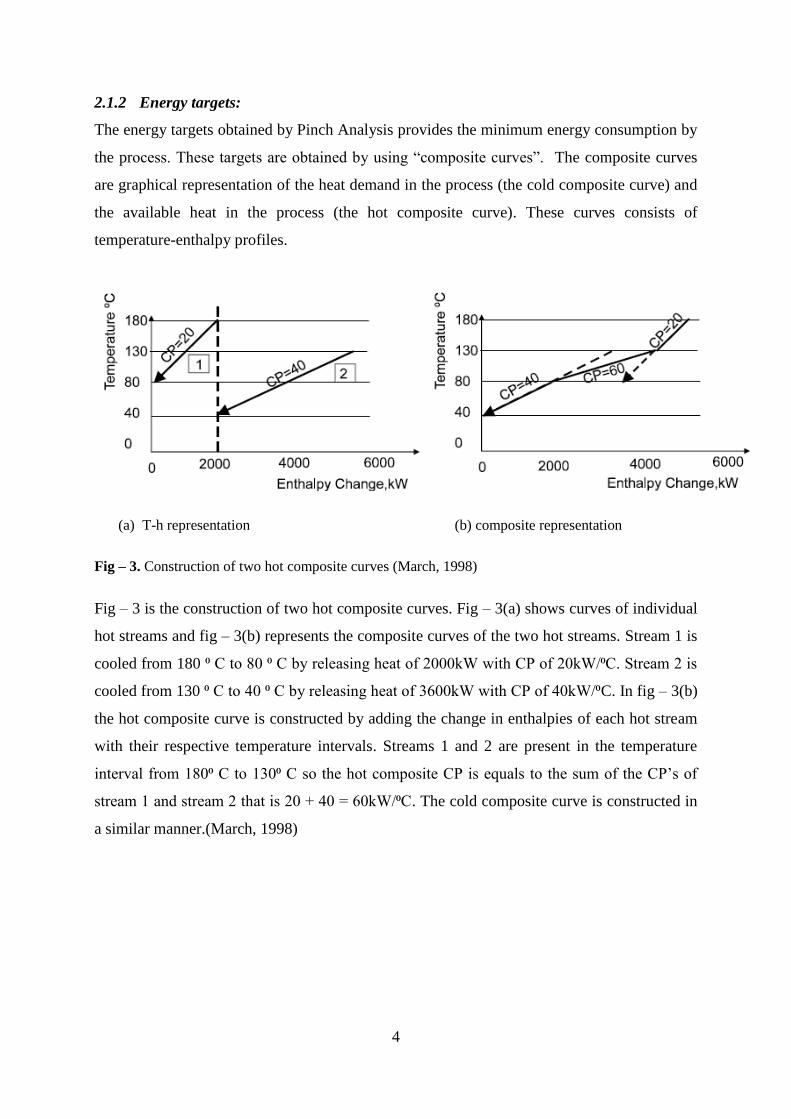
2.1.2 Energy targets:
The energy targets obtained by Pinch Analysis provides the minimum energy consumption by
the process. These targets are obtained by using “composite curves”. The composite curves
are graphical representation of the heat demand in the process (the cold composite curve) and
the available heat in the process (the hot composite curve). These curves consists of
temperature-enthalpy profiles.
(a) T-h representation (b) composite representation
Fig – 3. Construction of two hot composite curves (March, 1998)
Fig – 3 is the construction of two hot composite curves. Fig – 3(a) shows curves of individual
hot streams and fig – 3(b) represents the composite curves of the two hot streams. Stream 1 is
cooled from 180 ⁰ C to 80 ⁰ C by releasing heat of 2000kW with CP of 20kW/⁰C. Stream 2 is
cooled from 130 ⁰ C to 40 ⁰ C by releasing heat of 3600kW with CP of 40kW/⁰C. In fig – 3(b)
the hot composite curve is constructed by adding the change in enthalpies of each hot stream
with their respective temperature intervals. Streams 1 and 2 are present in the temperature
interval from 180⁰ C to 130⁰ C so the hot composite CP is equals to the sum of the CP’s of
stream 1 and stream 2 that is 20 + 40 = 60kW/⁰C. The cold composite curve is constructed in
a similar manner.(March, 1998)
5
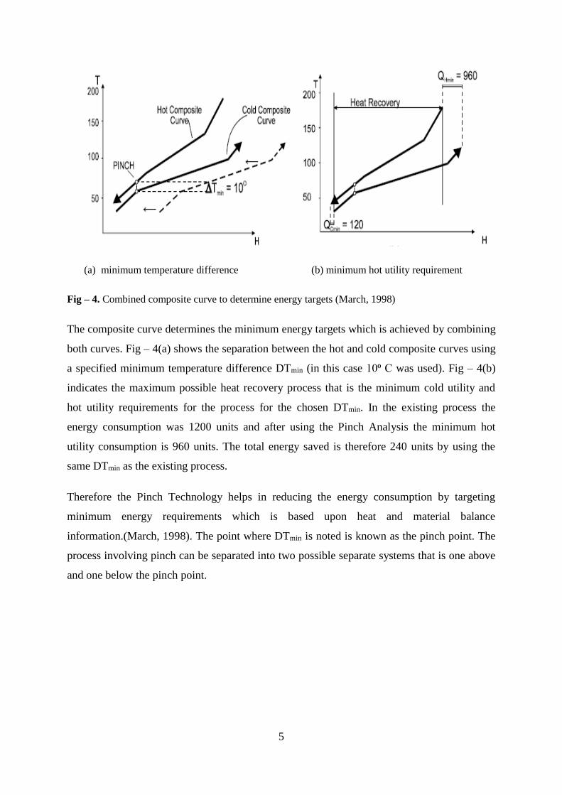
(a) minimum temperature difference (b) minimum hot utility requirement
Fig – 4. Combined composite curve to determine energy targets (March, 1998)
The composite curve determines the minimum energy targets which is achieved by combining
both curves. Fig – 4(a) shows the separation between the hot and cold composite curves using
a specified minimum temperature difference DTmin (in this case 10⁰ C was used). Fig – 4(b)
indicates the maximum possible heat recovery process that is the minimum cold utility and
hot utility requirements for the process for the chosen DTmin. In the existing process the
energy consumption was 1200 units and after using the Pinch Analysis the minimum hot
utility consumption is 960 units. The total energy saved is therefore 240 units by using the
same DTmin as the existing process.
Therefore the Pinch Technology helps in reducing the energy consumption by targeting
minimum energy requirements which is based upon heat and material balance
information.(March, 1998). The point where DTmin is noted is known as the pinch point. The
process involving pinch can be separated into two possible separate systems that is one above
and one below the pinch point.
6
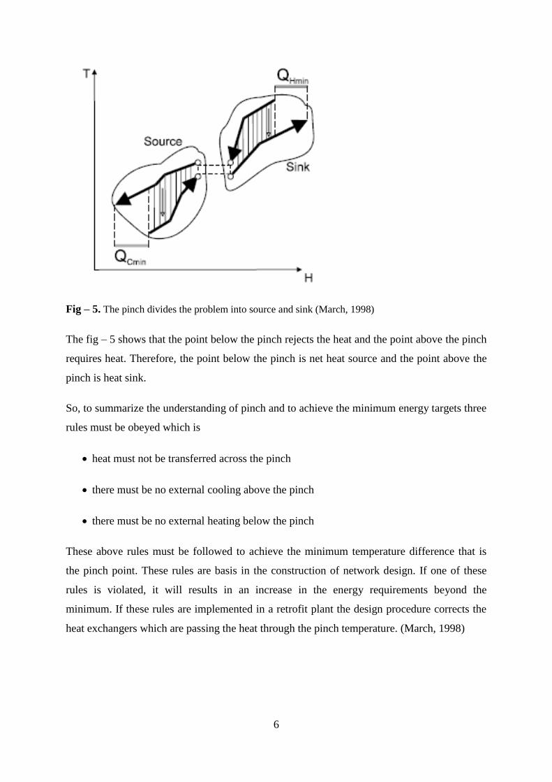
Fig – 5. The pinch divides the problem into source and sink (March, 1998)
The fig – 5 shows that the point below the pinch rejects the heat and the point above the pinch
requires heat. Therefore, the point below the pinch is net heat source and the point above the
pinch is heat sink.
So, to summarize the understanding of pinch and to achieve the minimum energy targets three
rules must be obeyed which is
heat must not be transferred across the pinch
there must be no external cooling above the pinch
there must be no external heating below the pinch
These above rules must be followed to achieve the minimum temperature difference that is
the pinch point. These rules are basis in the construction of network design. If one of these
rules is violated, it will results in an increase in the energy requirements beyond the
minimum. If these rules are implemented in a retrofit plant the design procedure corrects the
heat exchangers which are passing the heat through the pinch temperature. (March, 1998)
7
2.2 Methods:
There are few groups of methods which are used to achieve optimal heat exchanger
configuration and to achieve economical design. They are
2.2.1 Thermodynamic approach:
The designing of power plants are done in a traditional way in order to maximize the thermal
efficiency of the power plant. The analyses made by traditional methods are based on the first
and second law of thermodynamics. These analyses display the various thermal inefficiencies
of the system and sub systems of the plant. Certain heuristic rules are applied as soon as the
inefficiencies are identified. Once the best thermally efficient design is achieved the capital
cost of the plant is assessed.
The above approach lacks accuracy at it cannot give an optimal configuration or solution
since it did not take in to consideration of the complex interaction between the subsystems.
(Zhu, 1998)
2.2.2 Thermo-economic approach:
The thermo-economic approach is an extension of the thermodynamic approach where the
prices of each streams in the unit along with capital cost is included in the analysis. This
approach tries to give the best capital expenditure without compromising the thermal
efficiencies. In order to find the most economical operating cost this model uses NPL (Non-
Linear Programing) – optimisation. When this method is used in an existing process or plant it
still uses the trial and error method for addressing the structural changes.(Zhu, 1998)
2.2.3 Mathematical optimisation:
By using the mathematical optimisation method it is possible to have a super structure which
contains all the possible options such as exploring the benefits of both changes in parameters
and structural changes in the process. But there are few drawbacks in this optimisation
process that is this process needs a good initial starting value and also good feasible boundary
conditions for variable in order to achieve good solution. Also, the formulation is non-convex
and non-linear for a power plant process which interferes with optimisation process.
Therefore a better superstructure optimisation is required in order to satisfy all the conditions
in a systematic way.(Zhu, 1998)
8
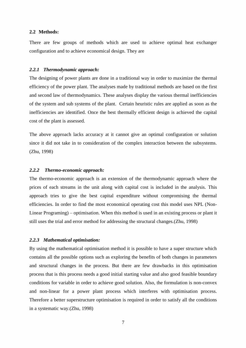
2.2.4 New methodology:
Fig – 6. Procedure for new methodology. (Zhu, 1998)
Fig – 6 shows the procedure for the new methodology which is the combination of benefits of
thermodynamic, thermos-economic and mathematic optimisation. There are two types of
design process in this design task which are analysis stage and design stage. The analysis
stages includes thermodynamic analysis, sensitive analysis and economic analysis
respectively. The function of analysis stage is to choose the best promising design options and
then evaluate them on the basis of thermal and economical performance of the plant. In the
design stage these promising designs are then implemented in a super structure. This supers-
structure to find out the best optimal configuration and parameters for the plant. (Zhu, 1998)
9
2.2.5 Enthalpy table algorithm method:
The enthalpy table algorithm method is a combination of pinch design method (PDM) and
problem table algorithm (PTA). The key feature of this technique is to design sub-networks of
heat exchangers. These sub-networks are placed on each enthalpy intervals of hot and cold
composite curves. These sub-networks are joined together to form into a single heat
exchanger network which is later simplified using pinch technology. This method follows few
steps to calculate the optimal solution. (Anastasovski, 2014)
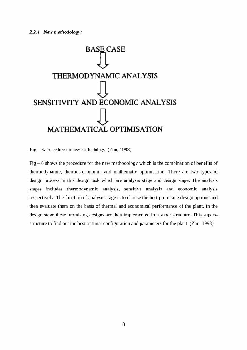
Step 1: determination of enthalpy and temperature intervals:
Table 1: stream data used for the enthalpy table algorithm (Anastasovski, 2014)
10
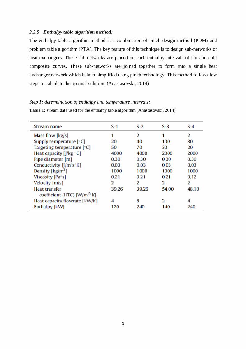
Fig – 7. Composite curve with enthalpy intervals (Anastasovski, 2014)
Table1 shows the enthalpy intervals and temperature intervals and fig – 7 shows that the
break points in the composite curve determines the enthalpy difference. One enthalpy interval
determines two different temperature intervals; one hot stream temperature interval and one
cold stream temperature interval. A linear interpolation was used to determine the missing
temperatures. The supply value of cold utility will be first temperature value for cold streams
at zero enthalpy. The hot and cold composite curve gives the known temperature values at the
next breaking point. In a situation where the hot stream temperature is unknown if the that
temperature is coming from cold stream’s target temperature, the breaking point of the cold
composite curve and the cold utility supply temperature gives the value.
Hinterval = ∆Tinterval * m * Cp -------------------------------- (eq – 1)
The above equation gives the enthalpy change where ∆Tinterval is interval temperature
difference of hot or cold stream, m is the total mass flow rate in the segment and Cp is the
average specific heat in that segment. (Anastasovski, 2014)

11
Step 2: creating a table of streams present in respective temperature intervals:
Table 2 – Heat capacity flow rates of energy streams. (Anastasovski, 2014)
Table2 shows the stream present in each temperature intervals. In table 2 it can be noted that
there are empty spaces which means that there are no stream present in those intervals. The
top row of streams can in this case be matched with hot utilities as it only contains cold
streams. Correspondingly, the bottom rows of hot streams can be satisfied with the cold
utilities. Hot or cold utilities are needed to be added if there are any unbalanced temperature
intervals. (Anastasovski, 2014)
Step 3: Construction of heat loads:
Table 3 – Heat content of energy streams present in certain temperature intervals. (Anastasovski,
2014)
Table-3 shows list of streams based upon heat content of streams which is present in certain
energy intervals. From the previously mentioned eq 1 the enthalpy are calculated and are

12
written in columns for all four streams. Heat balances for every stream is represented in the
last column, in which all balances are zero except the ones in the top and bottom. The heating
and cooling demands are represented by the heat values in those positions. Negative sign is
given to hot streams since they give out heat or energy and cold streams with positive sign
since they accept heat. (Anastasovski, 2014)
Step 4: design of a primary heat exchanger network:
In table – 5 almost all the enthalpies are balanced and the places where the enthalpies are not
balanced are represented by hot and cold utilities. The sub networks are independent problems
so their starting point in the design can be from any interval. All sub-networks are connected
in the same way as it represented in the combined composite curve. The heat load of each
stream is compared to the highest of all its values. The streams which have the same heat load
values are paired. If a single heat exchanger is added between the hot and cold streams, it can
be noted that there is no violation of ∆Tmin. The problem comes in by pairing a second heat
exchanger which is placed between the non-paired parts of the stream fragments where the
possibility of series connection must be checked. Series connection means that heat from one
hot stream is transferred to more than one cold stream. The design direction can be started
from right side to left side or from left side to right side. The new supply temperature must be
determined if the design direction starts from right side to left side. The new supply
temperature is determined by the value of heat that is transferred from hot stream to cold
stream. If the streams are connected from left side to right side, the new supply temperature
for the cold stream must be higher than or equal to cold streams target temperature.
(a) Left to right direction design for cold utility demand.
13
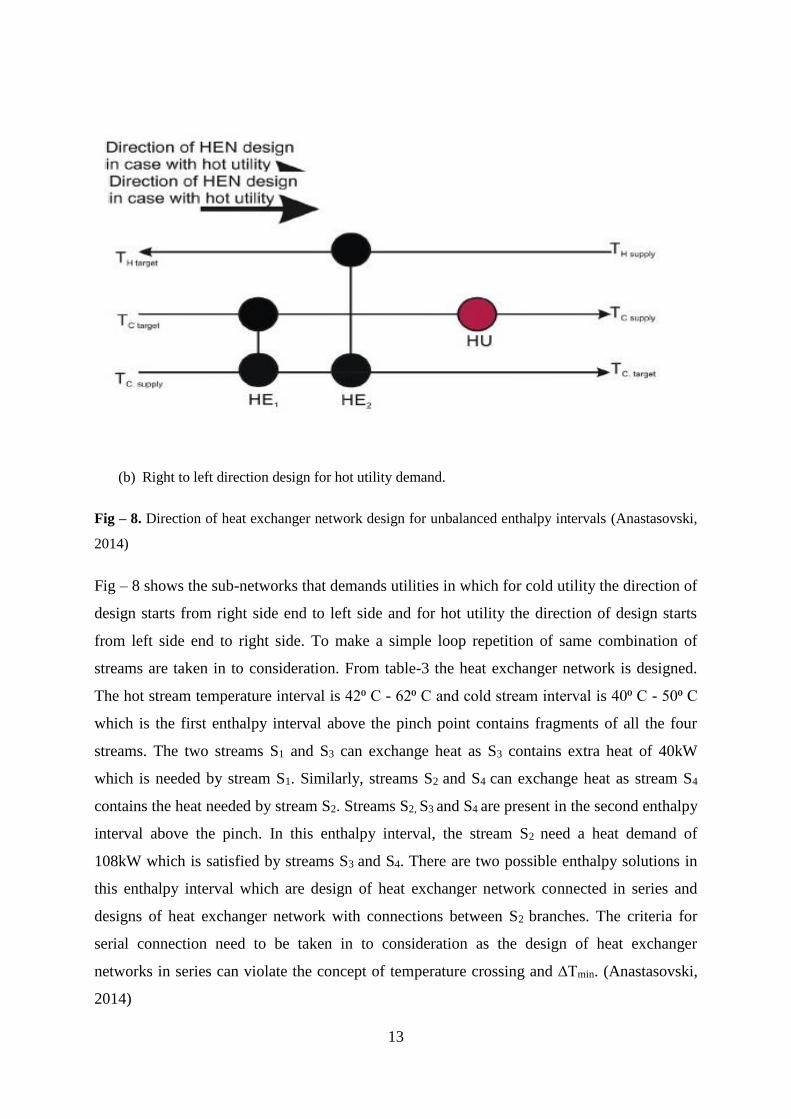
(b) Right to left direction design for hot utility demand.
Fig – 8. Direction of heat exchanger network design for unbalanced enthalpy intervals (Anastasovski,
2014)
Fig – 8 shows the sub-networks that demands utilities in which for cold utility the direction of
design starts from right side end to left side and for hot utility the direction of design starts
from left side end to right side. To make a simple loop repetition of same combination of
streams are taken in to consideration. From table-3 the heat exchanger network is designed.
The hot stream temperature interval is 42⁰ C - 62⁰ C and cold stream interval is 40⁰ C - 50⁰ C
which is the first enthalpy interval above the pinch point contains fragments of all the four
streams. The two streams S1 and S3 can exchange heat as S3 contains extra heat of 40kW
which is needed by stream S1. Similarly, streams S2 and S4 can exchange heat as stream S4
contains the heat needed by stream S2. Streams S2, S3 and S4 are present in the second enthalpy
interval above the pinch. In this enthalpy interval, the stream S2 need a heat demand of
108kW which is satisfied by streams S3 and S4. There are two possible enthalpy solutions in
this enthalpy interval which are design of heat exchanger network connected in series and
designs of heat exchanger network with connections between S2 branches. The criteria for
serial connection need to be taken in to consideration as the design of heat exchanger
networks in series can violate the concept of temperature crossing and ∆Tmin. (Anastasovski,
2014)

14
step 5: simplifying of networks to the final design of heat exchanger network:
(a) The case with branching of stream fragments with marked loops according to pinch
technology rule
(b) Cases with marked loops and paths that are going through the pinch point
Fig – 9. Grid diagram of designed heat exchanger networks. (Anastasovski, 2014)
In fig – 9 there can be noted some loops and paths to get a new form, in which there is loop
between the path that connects heaters and cooler and heat exchangers HE4 and HE6. the
heat exchangers HE3 and HE5 are second loop and heat exchangers HE7 and HE8 are third
loop. By summing the heat load of every heat exchanger of that loop, new heat exchangers are
created.

15
Fig – 10. Heat exchanger network after using of rule for loops through the pinch point. (Anastasovski,
2014)
From fig – 10 it can be noted that there is a reduction in the energy required by the hot and
cold utility. There will be a violation of ∆Tmin, if the path that goes to heat exchanger 5 is
broken.
This is technique can be used in threshold problems or multiple pinch problems. This
technique divides the networks in to sub-networks and the break points in the hot and cold
composite curve determines the number of sub-networks. This method gives the continuity of
process streams in the network design as there is a possibility of pairing up of already paired
stream combinations. There is a possibility of increasing the number of loops which gives a
simple solution.
There are some drawbacks in this method as it depends on the designers ability to solve the
problem and creativity of the designer. (Anastasovski, 2014)
2.2.6 The extended pinch analysis method for sub ambient process:
The extended pinch analysis deals with exergy analysis which has the advantages of including
all the stream properties such as temperature, pressure and composition. The methodology of
this process is the combination of the pinch analysis and exergy analysis to find the minimum
annual cost with the use of mathematic programming. Situations such as when supply
pressure (Ps) greater than the target pressure (Pt) a favourable design procedure was
developed. In this method, the compression and expansion work is optimised together with
the work needed to create the cooling utilities. In a sub-ambient process the temperature of a
stream is decreased when the stream is expanded as the pressure is reduced and at the same
16
time cooling duty of the stream is increased. Thus, some of the original pressure based exergy
is converted to temperature based exergy. (Aspelund et al., 2007)
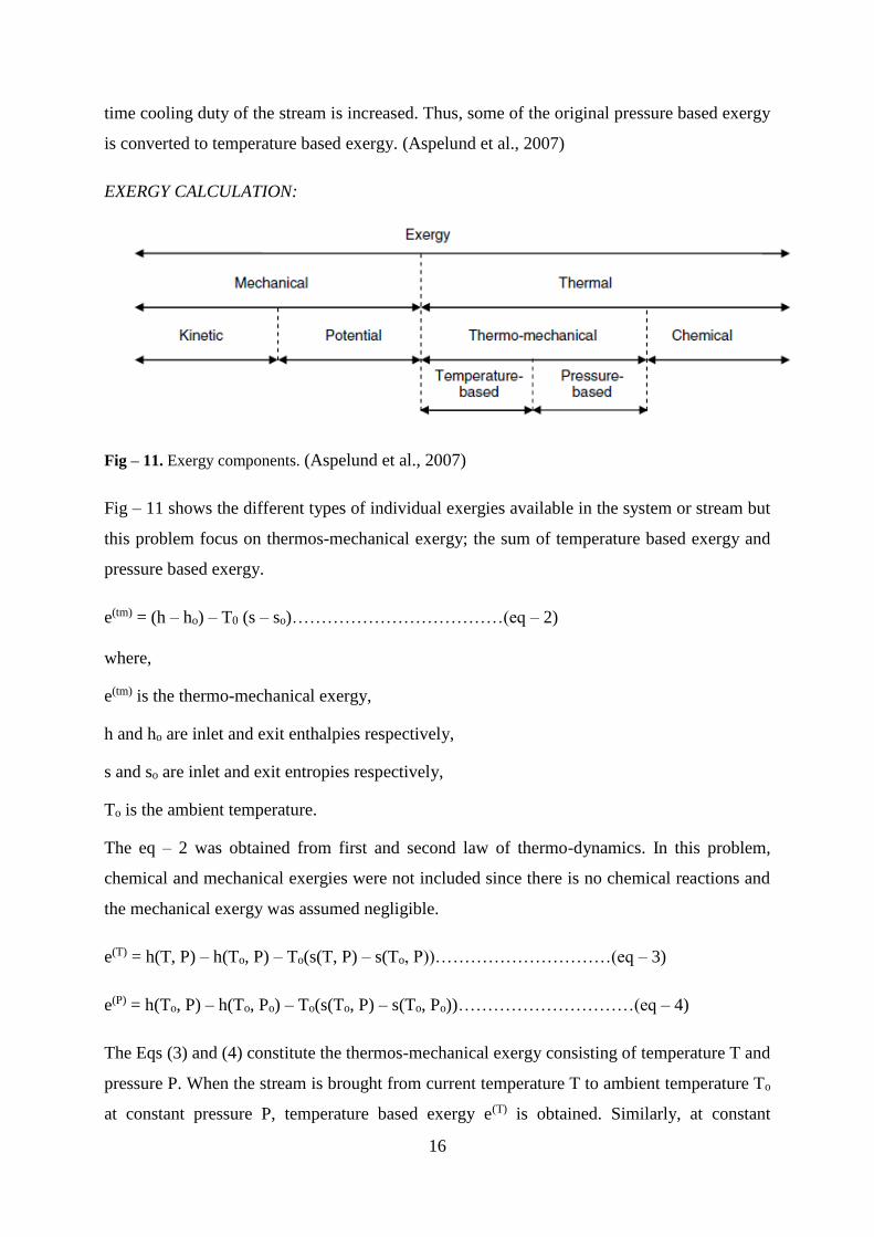
EXERGY CALCULATION:
Fig – 11. Exergy components. (Aspelund et al., 2007)
Fig – 11 shows the different types of individual exergies available in the system or stream but
this problem focus on thermos-mechanical exergy; the sum of temperature based exergy and
pressure based exergy.
e(tm) = (h – ho) – T0 (s – so)………………………………(eq – 2)
where,
e(tm) is the thermo-mechanical exergy,
h and ho are inlet and exit enthalpies respectively,
s and so are inlet and exit entropies respectively,
To is the ambient temperature.
The eq – 2 was obtained from first and second law of thermo-dynamics. In this problem,
chemical and mechanical exergies were not included since there is no chemical reactions and
the mechanical exergy was assumed negligible.
e(T) = h(T, P) – h(To, P) – To(s(T, P) – s(To, P))…………………………(eq – 3)
e(P) = h(To, P) – h(To, Po) – To(s(To, P) – s(To, Po))…………………………(eq – 4)
The Eqs (3) and (4) constitute the thermos-mechanical exergy consisting of temperature T and
pressure P. When the stream is brought from current temperature T to ambient temperature To
at constant pressure P, temperature based exergy e(T) is obtained. Similarly, at constant

17
temperature To, if the stream is brought from initial pressure P to ambient pressure Po,
pressure based exergy e(P) is obtained.
Ec.min = ∆Ec = ∆E(TH - ∆T)
= ṁCp [TH.s - TH.t – To ln ((TH.s - ∆T) / (TH.t - ∆T))]…………………(eq – 5)
Eq – 5 shows the minimum amount of exergy Ec.min required to cool down a hot stream at
constant ∆T by heat transfer. Where, TH.s and TH.t are the hot stream at sub-ambient supply
temperature and hot stream at sub-ambient target temperature respectively. (Aspelund et al.,
2007)
The overall design procedures are, (Aspelund et al., 2007)
The total exergy of hot and cold streams is calculated to check whether it is possible to
have a process without utilities or not. If the calculated exergy is above 100%
minimum energy required is found.
After finding out the minimum temperature differences and equipment efficiencies
establish an initial estimate for the irreversibility’s.
To find the pinch point and minimum amount of heat required by hot and cold
utilities, develop the hot and cold streams composite curves.
After the expansion and compression process of the process stream, develop the pinch
curves.
Calculate new exergy efficiency.
Compare the new exergy with the old one and develop the current design with new
exergy efficiency.
This procedure does not guarantee global optimal solution.

18
Fig – 12. Procedure for cooling a hot stream by utilizing pressure based exergy in a cold stream.
(Aspelund et al., 2007)
A simplified version of the procedure for cooling a hot stream by using exergy in a cold
stream is shown in fig – 12. The first step is to modify the hot and cold stream temperature
using the Pinch Analysis. The hot and cold stream temperatures are adjusted by subtracting
half of ∆Tmin for hot stream and adding half of ∆Tmin for cold stream. The cold stream is
compressed to reach the hot stream target temperature if the original cold stream is colder
than the hot stream target temperature. This process helps to reduce the exergy loss. While
compressing the cold stream, some work is needed, which is recovered by expansion by
producing additional cooling at high temperature. In some cases, the cold stream is expanded
if the cold stream supply temperature is higher than the hot stream target temperature.
(Aspelund et al., 2007)

19
In step (2) the heat capacity flow rates of hot and cold streams are compared. In this step the
hot stream target temperature is higher than the new cold stream temperature. The composite
curve will diverge and the cross-over in the cold region is avoided if the flowrate of the total
heat capacity of the cold stream is equal to or larger than that of the hot stream in the cold
region. To increase the total heat capacity flow rate of the cold stream, the cold stream is
expanded several times. Depending on the total enthalpy changes and the energy content of
the stream, external heating and cooling systems are added.
In the step (3) one more expansion is done, if there is any pressure available in the cold
stream. To make the composite curve diverge at least one more sub-stream is needed in the
cold end.
In step (4) to maintain equal pressure ratio over the expanders. But by following this step the
inlet temperatures must be increased to obtain the target outlet temperature if the pressure
ratio across the expanders are decreased. Step (5) indicates the need for external cooling
utility if the cold end cannot be solved due to lack of expanders.
The above method is a promising tool to achieve an optimal solution to develop the energy
intensive process. This methodology uses both the traditional pinch analysis and exergy
analysis to give an optimal solution in a transparent way. (Aspelund et al., 2007)
2.2.7 A graphical method for pinch analysis:
In this method, a graph is constructed for representing an existing heat exchanger network by
plotting the temperatures of process hot streams versus temperatures of cold streams. Straight
lines are drawn to represent the existing heat exchanger. From these straight lines slopes are
drawn which is proportional to the ratio of heat capacities and flow. The conventional method
is has some difficulty in matching the existing temperatures with the target values of the
curves. But by using the new graphical method it’s easier to achieve the energy targets and in
estimating the performance of the heat exchanger network. (Gadalla, 2015)
20
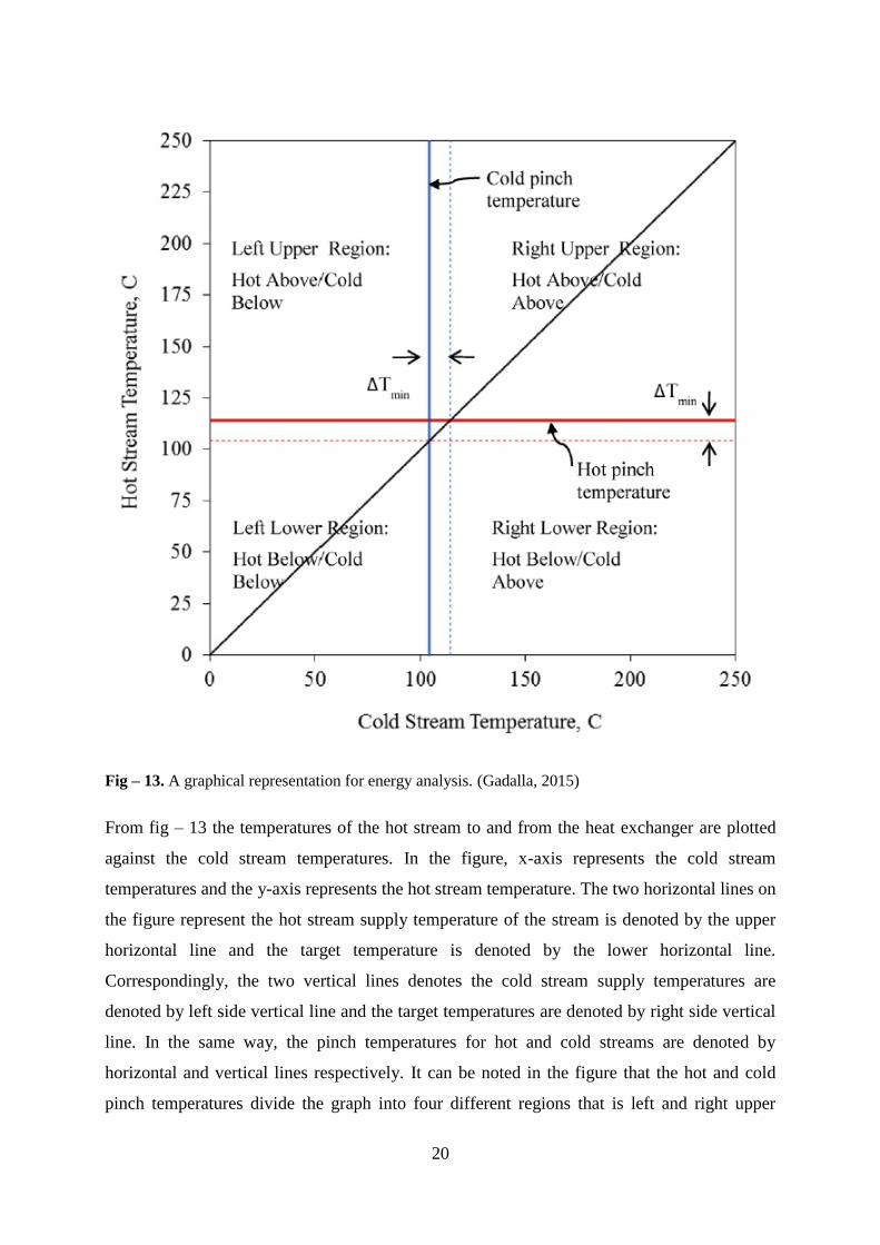
Fig – 13. A graphical representation for energy analysis. (Gadalla, 2015)
From fig – 13 the temperatures of the hot stream to and from the heat exchanger are plotted
against the cold stream temperatures. In the figure, x-axis represents the cold stream
temperatures and the y-axis represents the hot stream temperature. The two horizontal lines on
the figure represent the hot stream supply temperature of the stream is denoted by the upper
horizontal line and the target temperature is denoted by the lower horizontal line.
Correspondingly, the two vertical lines denotes the cold stream supply temperatures are
denoted by left side vertical line and the target temperatures are denoted by right side vertical
line. In the same way, the pinch temperatures for hot and cold streams are denoted by
horizontal and vertical lines respectively. It can be noted in the figure that the hot and cold
pinch temperatures divide the graph into four different regions that is left and right upper
21
regions and left and right lower regions. These regions represent the possible exchanger
matches within the heat exchanger network, which are as follows, (Gadalla, 2015)
The left upper region shows that there is heat exchange between the hot streams
above the pinch point and the cold stream below the pinch point.
The right upper region shows that there is heat exchange between hot streams above
the pinch point and the cold streams above the pinch point.
The left lower region shows that there is heat exchange between hot streams below
the pinch point and the cold streams below the pinch point.
The right lower region shows that there is heat exchange between hot streams below
the pinch point and the cold streams above the pinch point.
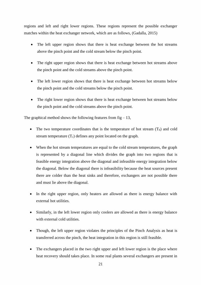
The graphical method shows the following features from fig – 13,
The two temperature coordinates that is the temperature of hot stream (Th) and cold
stream temperature (Tc) defines any point located on the graph.
When the hot stream temperatures are equal to the cold stream temperatures, the graph
is represented by a diagonal line which divides the graph into two regions that is
feasible energy integration above the diagonal and infeasible energy integration below
the diagonal. Below the diagonal there is infeasibility because the heat sources present
there are colder than the heat sinks and therefore, exchangers are not possible there
and must lie above the diagonal.
In the right upper region, only heaters are allowed as there is energy balance with
external hot utilities.
Similarly, in the left lower region only coolers are allowed as there is energy balance
with external cold utilities.
Though, the left upper region violates the principles of the Pinch Analysis as heat is
transferred across the pinch, the heat integration in this region is still feasible.
The exchangers placed in the two right upper and left lower region is the place where
heat recovery should takes place. In some real plants several exchangers are present in
22
the left upper region, which indicates inefficient heat recovery designs. As the result
of the inefficient design more fuels and utilities are consumed.
The heat exchanger matches that touch the pinch temperatures signifies that the energy
integration takes place across the pinch temperatures.
The graphical method can represent the heat exchangers as temperatures of hot streams
plotted against the temperatures of cold streams. This method can evaluate the performance of
existing heat exchanger networks with respect to pinch analysis by identifying the
inefficiencies of the process. Further, this method reduces the energy demand by the utilities
by shifting heat graphically between heat exchanger loops. (Gadalla, 2015)
2.2.8 Biogeography – based optimization method:
Simon proposed the biogeography algorithm method which is a new and powerful
optimization technique. The study of geographical distribution of biological organisms is
called biogeography. The geographical areas which are suitable for the biological species said
to have a high habitat suitability index (HSI). There certain variables called suitability index
variables (SIVs) which characterize the habitability of species. The HSI and SIV are
considered as dependent and independent variables respectively. A higher habitat suitability
index, means a lager the number of species. The habitats having higher HSI are more stable
than the habitats with lower HSI. This technique is based upon migration and mutation. The
mathematic representation of migration and mutation are as follows, (Hadidi and Nazari,
2013)
Migration:
This method is similar to that of other population optimization technique. The solutions of
candidate are represented as vector of real numbers in which each real numbers are
considered as one SIV in the array. In biogeography based optimization (BBO), the quality of
each candidate solution is found using HSI. Higher the HSI solution, better the quality of
solution and lower the HSI solution, lower the quality of solution. To share information
between habitats probabilistically, the rates of emigration and immigration of each solution is
used. Each solution is modified using habitat modification probability. To modify suitability
index variable, immigration rate (λs) of each solution is used. To select which population set

23
will migrate, emigration rates (µs) are used probabilistically. The migration process brings
changes within the existing solution. (Hadidi and Nazari, 2013)
Mutation:
Some changes can occur suddenly due to natural calamities in the HSI of natural habitat
which causes some changes in the equilibrium value of the habitat. This process is called
mutation. The mutation rates are determined by species count probabilities.
Phs = - ( λs + µs )Ps + µs+1Ps+1 S = 0,----------------------------------------(eq – 6)
Phs = - ( λs + µs )Ps + λs-1Ps-1 + µs+1Ps+1 1 ≤ S ≤ Smax – 1,-------------------(eq – 7)
Phs = - ( λs + µs )Ps + λs-1Ps-1 S = Smax------------------------------------(eq – 8)
The above differential equations are used to calculate the probability of each species count.
Where,
Ps is the probability of habitat containing exactly S species,
Ps+1 is the probability of habitat containing S+1 species,
Ps-1 is the probability of habitat containing S-1 species,
λs, µs is the immigration and emigration rate of habitat containing S species,
λs-1, µs-1 is the immigration and emigration rate of habitat containing S-1 species,
λs+1, µs+1 is the immigration and emigration rate of habitat containing S+1 species,
Smax is the maximum species count.
Higher the probability of the solution, lower the chance of mutation and similarly, lower the
probability of the given solution, higher the chance of mutation. So better values are obtained
with medium HSI solution.
Based on this method there was reduction in capital cost up to 14% and savings in operating
costs up to 96%. So the over decrease of total cost was up to 56.1% by using the
biogeography based optimization. (Hadidi and Nazari, 2013)

24
2.2.9 Particle swarm optimization (PSO):
The particle swarm optimization is based upon superstructure simulation optimization model
by including steam splitting to minimize the total annual cost and energy cost of utilities. This
method was developed by Kennedy and Eberhart in 2001, where they got stirred by the social
behaviour of bird flocking or fish schooling. The technique used in the PSO process is
stochastic optimisation technique. The procedure provided by particle swarm optimization is
population based search procedure in which the particles change their position or state with
time. Each particle in the PSO system fly’s around in a multi-dimensional search space where
the position is adjusted according to its own experience and the experience of the
neighbouring particles to make sure the possible best position is occupied by all particles. In
most of the research and application areas the PSO is implemented successfully. In the PSO,
only few parameters are need to be adjusted and therefore it became attractive in different
research areas. The objective function used in this case is as follows (Silva et al., 2009)
Minimize Cglobal = (CHU . HU + CCU . CU) + Σ (a +b. Akc)……………….(eq – 9)
Where, HU, CU, CHU are hot and cold utilities and the cost associated to them a, b and c
which are constants that depend on the equipment used, A is the area of heat exchanger.
υk+1(i) = ωkυk+1
(i) + c1r1(рk(i) – xk
(i)) + c2r2(рkglobal – xk
(i))………………………..(eq – 10)
xk+1(i) = xk
(i) + υk+1(i)………………..(eq – 11)
Where,
xk(i) and υ(i) are position and velocity vectors of the particle i, respectively,
ωk is the inertia weight,
c1 and c2 are constants,
r1 and r2 are two random vectors,
k is the iteration number,
рk(i) is the position with best result of particle i,
рkglobal is position with best result of the group.
According to eq – 5 and eq – 6, the particles and the velocity of each particle are actualised.
At the beginning of the optimization, the variables are randomly generated and then the
location is modified. The particles are formed based on variables such as number of stages,

25
heat exchanged in each equipment, fraction of cold stream splitting and fraction of hot stream
splitting. The hot and cold utilities demand and the heat exchangers areas are calculated after
the generation of the particle. The hot and cold utilities demand and the heat exchangers areas
are calculated after the generation of the particle The objective function is penalized, if the
particle is not a solution of the problem or if the particle violates any constrains. (Silva et al.,
2009)
2.2.10 The R-curve analysis method:
Kimura and Zhu developed the R-curve analysis method to determine the most economic
modifications to existing utility systems. The R-curve is a curve which indicates of exixting
plant can be improved without any capital investment. By converting the fuel energy into heat
(Qheat) and power (W), a target for the efficiency of utility system is provided by the R-curve.
A heat sink is required for the production of shaft work from fuel energy; this fact determines
the shape of the R-curve. The ratio of useful part of energy and the integrated energy
consumption (Qfuel) is the fuel utilisation efficiency or integrated energy efficiency. The
process plant acts as the heat sink for power generation in an integrated site. The overall
generation becomes more efficient if the heat demand to power demand is large.
Fig – 14. Theoretical limit lines of two energy curve. (Matsuda et al., 2009)

26
Fig – 14 determines the theoretical lines of the two energy systems. In the above figure the
two energy systems used are gas turbine combined system and boiler and turbine
conventional system. Maximum achievable efficiency is shown by the R-curve for the given
R-ratio. The R-ratio is the ratio of power to the heat demand from the process. A scope of
improvement in the design is revealed in the difference between the existing efficiency and
maximum efficiency. To determine complex wide opportunities of multiple sites, the power
and heat demand of multiple sites are combined to form the R-curves. The R-curve is applied
on the basis of minimum energy requirement balance in a conventional approach. The R-
curve analysis estimates the amount of theoretical energy that can be saved and also estimates
the present condition of the utility systems.(Matsuda et al., 2009)
2.3 Genetic algorithm:
The optimization process consists of forming an initial basic concept and improving the
concept based upon gained information to find the maximum or minimum output results. In
the optimization process the input may be a variable or functions such as objective function or
cost function or fitness function (Haupt and Haupt, 2003).
There are different types of optimization technique but the most commonly used technique to
find the global minimum or maximum is genetic optimization. In 1960, Genetic Algorithm
(GA) was invented by John Holland and later in the year 1960s and 1970s the algorithm was
developed by Holland and his students and colleagues at the University of Michigan. Original
goal was to design an algorithm to understand the phenomenon of nature adaptation and to
find ways to implement this process into computer systems (Mitchell, 1996). Generally
speaking, genetic algorithms are probabilistic optimization methods in which the concept of
evolution is used to improve the solution to find better global minimum or maximum value
(Bodenhofer, October,2003).
In the genetic algorithm, to a given problem or process each individual represents a possible
solution where the individuals are determined randomly from search space. The fitness
function or objective function determines the result of the variable that needs to be optimized
to find the fitness of the solution. The next generation of population is determined by the
individuals that has the best fitness solution within the previous population. An optimal
solution is obtained for a given problem from the group of possible solutions.
(M.A.S.S.Ravagnani, June, 2005)

27
Fig – 15. Genetic operation for each generations.(Ravagnani et al., 2005)
Fig – 14 shows a simplified flow-chart about different operations in a genetic algorithm. In
the genetic algorithm, the transition from one generation to next generation consists of three
basic process; which are,
Selection:
In the selection process, per the fitness or objective function value, individuals are
selected for reproduction.
Cross-over:
Two individual containing genetic information or coding are merged together to
produce good children or solution in this process.
Mutation:
The mutation is the process in which random deformation of strings occurs with a
certain probability to avoid local maxima. (Bodenhofer, October,2003)
28
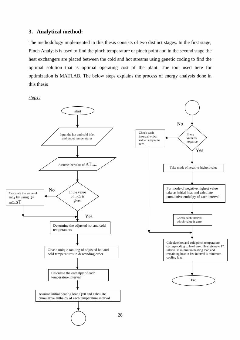
3. Analytical method:
The methodology implemented in this thesis consists of two distinct stages. In the first stage,
Pinch Analysis is used to find the pinch temperature or pinch point and in the second stage the
heat exchangers are placed between the cold and hot streams using genetic coding to find the
optimal solution that is optimal operating cost of the plant. The tool used here for
optimization is MATLAB. The below steps explains the process of energy analysis done in
this thesis
step1:
No
Yes
No
Yes
start
Input the hot and cold inlet and outlet temperatures
Assume the value of ∆Tmin
If the value
of mCp is
given
Calculate the value of
mCp by using Q=
mCp∆T
Determine the adjusted hot and cold
temperatures
Give a unique ranking of adjusted hot and
cold temperatures in descending order
Calculate the enthalpy of each
temperature interval
Assume initial heating load Q=0 and calculate
cumulative enthalpy of each temperature interval
If any value is
negative
Check each
interval which value is equal to
zero
Take mode of negative highest value
For mode of negative highest value
take as initial heat and calculate
cumulative enthalpy of each interval
Check each interval
which value is zero
Calculate hot and cold pinch temperature corresponding to load zero. Heat given to 1st
interval is minimum heating load and
remaining heat in last interval is minimum cooling load
End

29
The above flow chart explains the steps in Pinch Analysis (Tewari et al., 2015). In the Pinch
Analysis step, the actual steam temperatures are converted to interval temperatures using the
below equations,
Hot streams Tint = Tact - ∆Tmin/2………………(eq – 12)
Cold streams Tint = Tact + ∆Tmin/2………………(eq – 13)
Where, Tint is the interval temperature, Tact is the actual temperature, ∆Tmin is the minimum
temperature difference. The minimum temperature difference is assumed and interval
temperature is calculated.
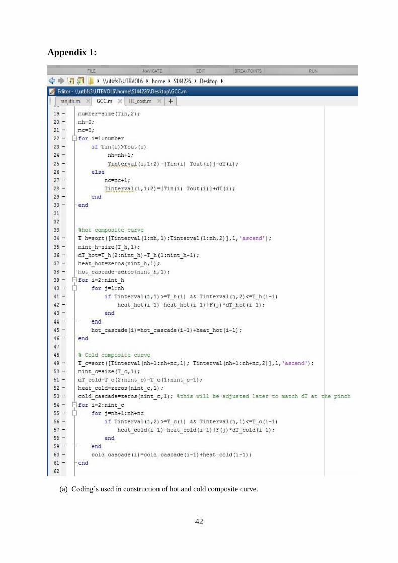
From appendix–1 shows the codes which are used to in the construction of hot and cold
composite curve to implement the Pinch Analysis in MATLAB. The initial heating value is
assumed to be zero. After finding the temperature intervals, there will be some duplicate
temperatures, which are arranged in the order of magnitude. Heat balance is carried out for
streams within each temperature intervals. There will be few negative values which are
eliminated by introducing some heat.
The pinch analysis is used as a function file which will be used later for heat exchanger
network synthesis. The minimum temperature difference is added manually to find the
possible pinch temperatures. A grand composite curve is then constructed from merging the
hot and the cold composite curve in one graph. From the grand composite curve the pinch
temperature is determined.
Step2:
The equation for area of heat exchanger and cost function or objective function to run the
gene coding is implemented as a function in MATLAB. The equation for calculating area is
given below,
Q = UA∆Tlm W…………………………………….(eq – 14)
Q = ṁCp,h (Th,in - Th,out) = ṁCp,c (Tc,in – Tc,out) W……………………………………..(eq – 15)
∆Tlm = [(Th,in - Th,out) + (Tc,in – Tc,out)]/[ln((Th,in - Th,out)/ (Tc,in – Tc,out))]……………(eq – 16)
Where,
Q is the heat transfer rate (W),
U is the overall heat transfer co-efficient (W/Km2),
30
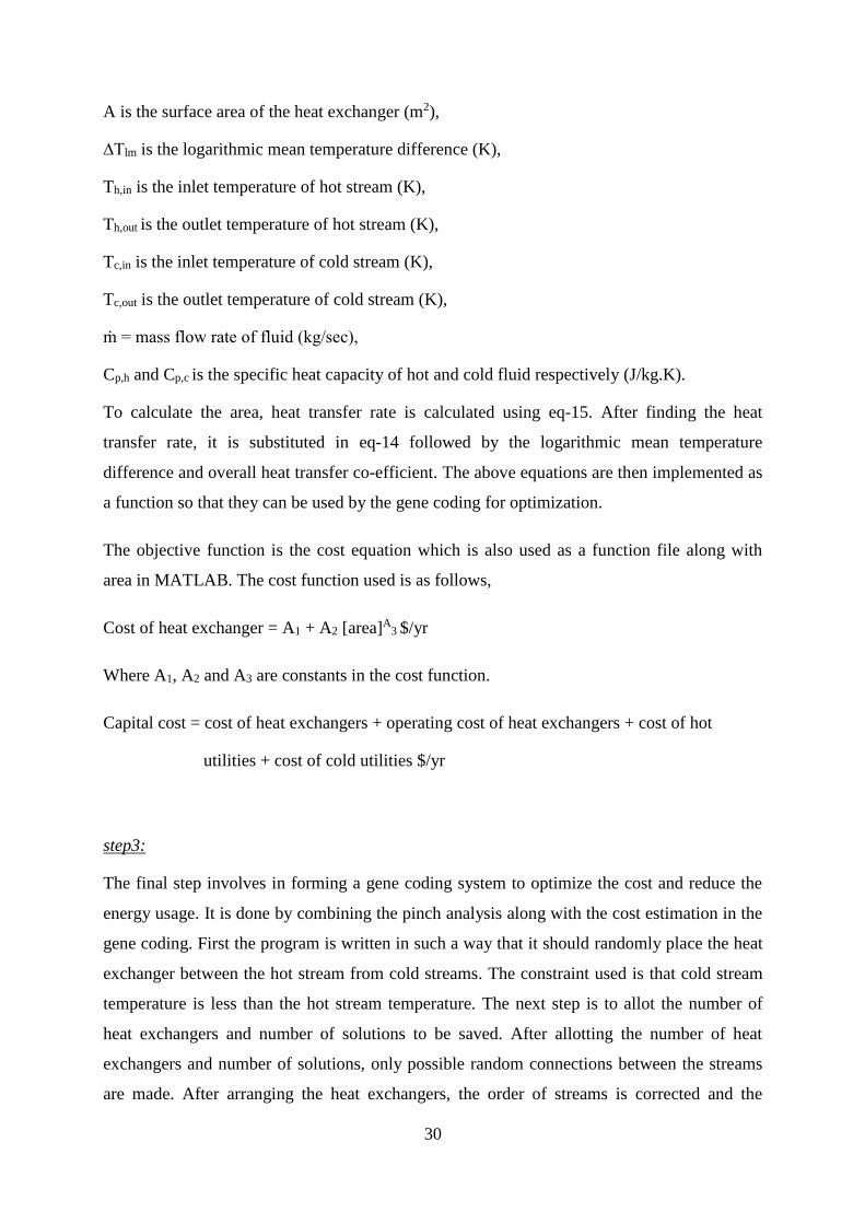
A is the surface area of the heat exchanger (m2),
∆Tlm is the logarithmic mean temperature difference (K),
Th,in is the inlet temperature of hot stream (K),
Th,out is the outlet temperature of hot stream (K),
Tc,in is the inlet temperature of cold stream (K),
Tc,out is the outlet temperature of cold stream (K),
ṁ = mass flow rate of fluid (kg/sec),
Cp,h and Cp,c is the specific heat capacity of hot and cold fluid respectively (J/kg.K).
To calculate the area, heat transfer rate is calculated using eq-15. After finding the heat
transfer rate, it is substituted in eq-14 followed by the logarithmic mean temperature
difference and overall heat transfer co-efficient. The above equations are then implemented as
a function so that they can be used by the gene coding for optimization.
The objective function is the cost equation which is also used as a function file along with
area in MATLAB. The cost function used is as follows,
Cost of heat exchanger = A1 + A2 [area]A3 $/yr
Where A1, A2 and A3 are constants in the cost function.
Capital cost = cost of heat exchangers + operating cost of heat exchangers + cost of hot
utilities + cost of cold utilities $/yr
step3:
The final step involves in forming a gene coding system to optimize the cost and reduce the
energy usage. It is done by combining the pinch analysis along with the cost estimation in the
gene coding. First the program is written in such a way that it should randomly place the heat
exchanger between the hot stream from cold streams. The constraint used is that cold stream
temperature is less than the hot stream temperature. The next step is to allot the number of
heat exchangers and number of solutions to be saved. After allotting the number of heat
exchangers and number of solutions, only possible random connections between the streams
are made. After arranging the heat exchangers, the order of streams is corrected and the
31
boundary conditions such as the lower limit and upper limits are set. And initial guesses are
made. The MATLAB function ‘fmincon’ is used to find the minimum cost based upon the
placement of heat exchangers. In this case the gene coding selects the individual streams
based upon the cost function and place the heat exchanger between the hot and cold streams.
In this particular case, cross-over is not included.
4. Results and discussion:
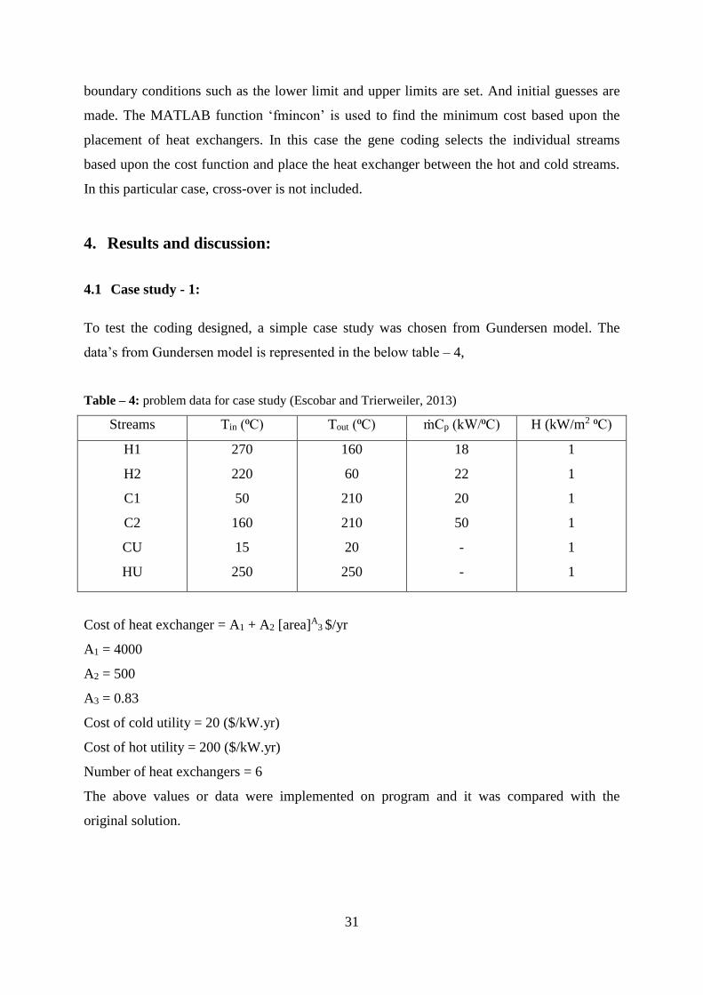
4.1 Case study - 1:
To test the coding designed, a simple case study was chosen from Gundersen model. The
data’s from Gundersen model is represented in the below table – 4,
Table – 4: problem data for case study (Escobar and Trierweiler, 2013)
Streams Tin (⁰C) Tout (⁰C) ṁCp (kW/⁰C) H (kW/m2 ⁰C)
H1
H2
C1
C2
CU
HU
270
220
50
160
15
250
160
60
210
210
20
250
18
22
20
50
-
-
1
1
1
1
1
1
Cost of heat exchanger = A1 + A2 [area]A3 $/yr
A1 = 4000
A2 = 500
A3 = 0.83
Cost of cold utility = 20 ($/kW.yr)
Cost of hot utility = 200 ($/kW.yr)
Number of heat exchangers = 6
The above values or data were implemented on program and it was compared with the
original solution.
32
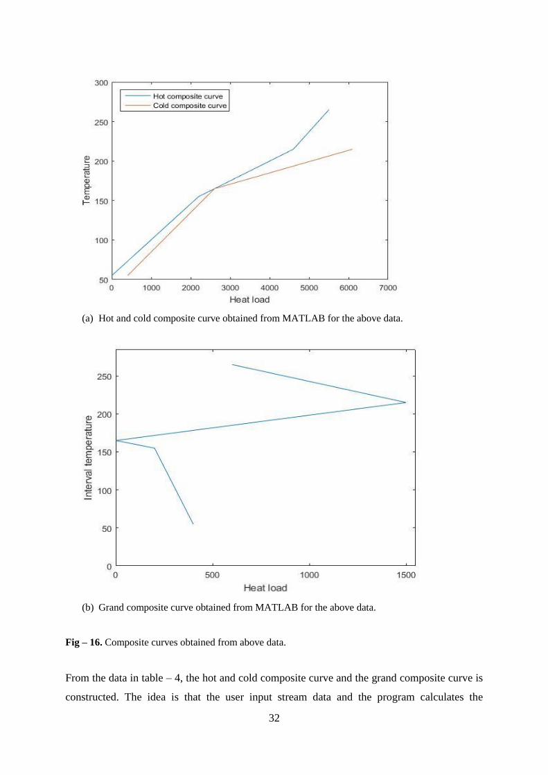
(a) Hot and cold composite curve obtained from MATLAB for the above data.
(b) Grand composite curve obtained from MATLAB for the above data.
Fig – 16. Composite curves obtained from above data.
From the data in table – 4, the hot and cold composite curve and the grand composite curve is
constructed. The idea is that the user input stream data and the program calculates the

33
minimum energy demand for cooling and heating as well as identifies the pinch point. In fig -
16 the x-axis heat load is plotted against the y-axis interval temperature to form the hot and
cold composite curve. The pinch point obtained for this case study is165 ⁰C.
(a) Actual placement of heat exchangers from reference model. (Escobar and Trierweiler, 2013)
(b) Obtained placement of heat exchanger from MATLAB.
Fig – 17. Comparison between the actual and obtained heat exchanger network.
34
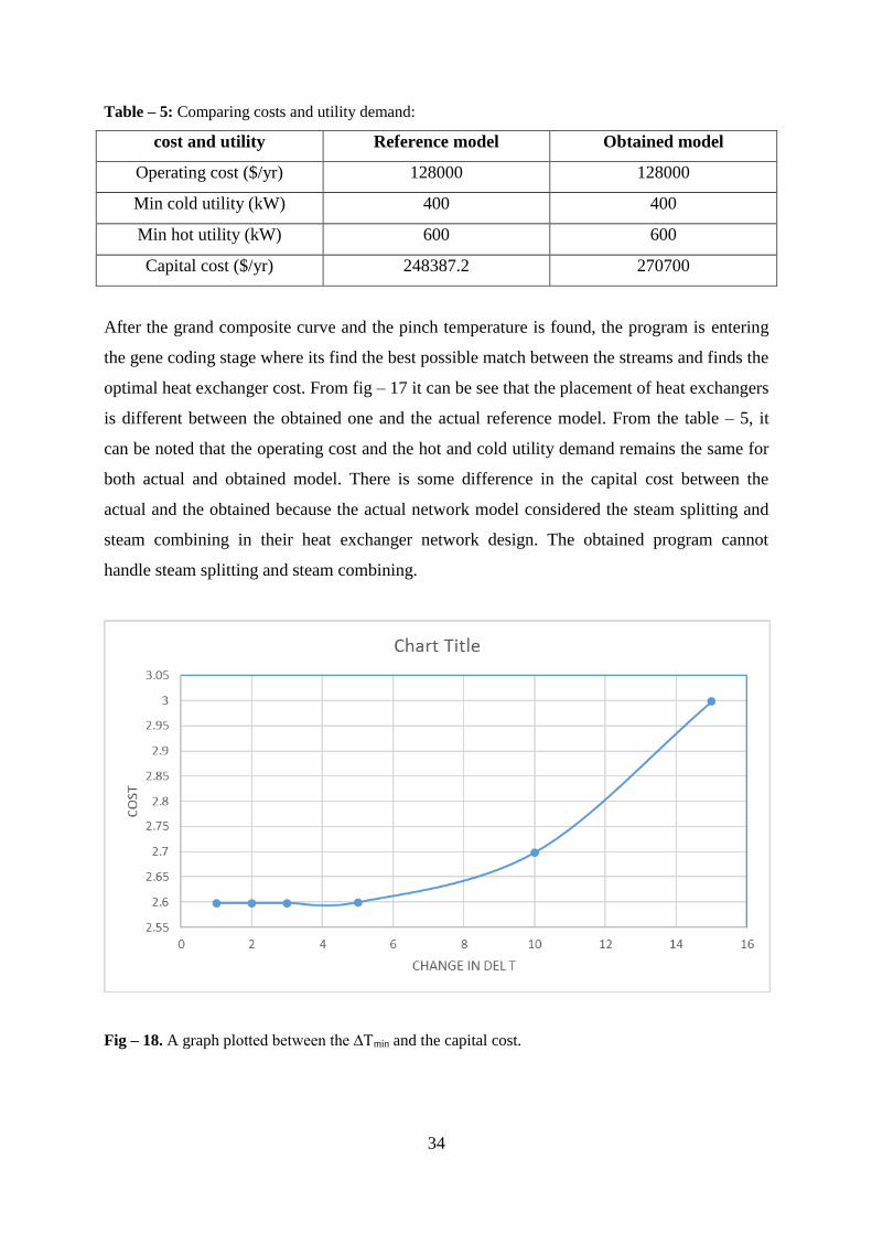
Table – 5: Comparing costs and utility demand:
cost and utility Reference model Obtained model
Operating cost ($/yr) 128000 128000
Min cold utility (kW) 400 400
Min hot utility (kW) 600 600
Capital cost ($/yr) 248387.2 270700
After the grand composite curve and the pinch temperature is found, the program is entering
the gene coding stage where its find the best possible match between the streams and finds the
optimal heat exchanger cost. From fig – 17 it can be see that the placement of heat exchangers
is different between the obtained one and the actual reference model. From the table – 5, it
can be noted that the operating cost and the hot and cold utility demand remains the same for
both actual and obtained model. There is some difference in the capital cost between the
actual and the obtained because the actual network model considered the steam splitting and
steam combining in their heat exchanger network design. The obtained program cannot
handle steam splitting and steam combining.
Fig – 18. A graph plotted between the ∆Tmin and the capital cost.

35
From fig – 18 it can be noted a graph is plotted between change in ∆Tmin and capital cost to
find the effects of ∆Tmin on the cost. From the graph, as ∆Tmin increases the cost increases but
below ∆Tmin = 6 the cost is constant or there are only minor changes in the value of cost. The
reason why a cost increase is not seen for small values of ∆Tmin in this optimization is that the
program optimizes with the target of minimizing the cost with a temperature difference of at
least ∆Tmin, but it does not require the specific temperature difference to be achieved.
4.2 Case study – 2:
In this case study the coding is tested against a complex design to check the capability the
coding against multiple heat exchangers and the time the MATLAB program took to find an
optimal solution. Same data from the Gunderson model were chosen but the number of heat
exchangers were increased.
Table – 6: Impact on cost due to number of heat exchangers and the time it took to find solution:
Number of heat
exchangers
Elapsed time (sec) Operating cost
($/yr)
Capital cost ($/yr)
8 246.1173 128000 269810
10 373.2784 128000 269810
12 403.3831 128000 270700
20 947.1394 128000 270700
From table-6 it can be noted that as the number of heat exchangers increases the time to find
the optimal solution also increases. The capital cost also increases as the number of heat
exchangers increases but becomes constant after adding more heat exchangers but the
operating cost remains the same.
36
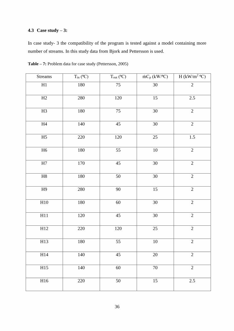
4.3 Case study – 3:
In case study- 3 the compatibility of the program is tested against a model containing more
number of streams. In this study data from Bjork and Pettersson is used.
Table – 7: Problem data for case study (Pettersson, 2005)
Streams Tin (⁰C) Tout (⁰C) ṁCp (kW/⁰C) H (kW/m2 ⁰C)
H1 180 75 30 2
H2 280 120 15 2.5
H3 180 75 30 2
H4 140 45 30 2
H5 220 120 25 1.5
H6 180 55 10 2
H7 170 45 30 2
H8 180 50 30 2
H9 280 90 15 2
H10 180 60 30 2
H11 120 45 30 2
H12 220 120 25 2
H13 180 55 10 2
H14 140 45 20 2
H15 140 60 70 2
H16 220 50 15 2.5
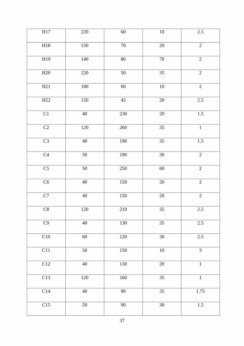
37
H17 220 60 10 2.5
H18 150 70 20 2
H19 140 80 70 2
H20 220 50 35 2
H21 180 60 10 2
H22 150 45 20 2.5
C1 40 230 20 1.5
C2 120 260 35 1
C3 40 190 35 1.5
C4 50 190 30 2
C5 50 250 60 2
C6 40 150 20 2
C7 40 150 20 2
C8 120 210 35 2.5
C9 40 130 35 2.5
C10 60 120 30 2.5
C11 50 150 10 3
C12 40 130 20 1
C13 120 160 35 1
C14 40 90 35 1.75
C15 50 90 30 1.5

38
C16 50 150 30 2
C17 30 150 50 2
CU 25 40 - 2
HU 325 325 - 1
Cost of heat exchanger = A1 + A2 [area]A3 $/yr
A1 = 8000
A2 = 800
A3 = 0.80
Cost of cold utility = 10 ($/kW.yr)
Cost of hot utility = 70 ($/kW.yr)
∆Tmin = 5
The above values or data were implemented on program and it was compared with the
original solution.
Table – 8: Comparing costs and utility demand:
cost and utility Reference model Obtained model
Operating cost ($/yr) 709000 715600
Cold utility (kW) 11740 11833
Hot utility (kW) 8460 8532.5
Capital cost ($/yr) 1998000 2723200
From table – 8, it can be noted that the operating cost and the hot and cold utility demand is
higher compared to the reference model. There is also huge difference in the capital cost and
the operating cost as the obtained program cannot handle steam splitting and steam
combining. In the obtained model 50 heat exchangers were used as a starting value and the
actual number of heat exchangers which were placed on the streams are 28.

39
Fig – 19. Heat exchanger network for multiple streams.
From fig – 19 it can be noted that the coding can find an optimal solution for multiple streams in this
case its 39 streams that is 22 hot streams and 17 cold steams.

40
Fig – 20. Grand composite curve from above data.
Fig – 20 shows the grand composite curve for the multiple stream case. From the fig it can be
seen that the minimum hot utility is 3375 kw and the minimum cold utility is 6675 kw.
5. Conclusions:
The most studied problems in the process synthesis is the heat exchanger network synthesis
but finding a feasible solution even for a small-scale problem has been troublesome. In this
work, the main optimization for the heat exchanger network and reduction of cost is carried
out using genetic algorithm or gene coding. The coding method implemented is tested on a
reference model which is simple that is consisting of four streams were chosen and the
obtained results were compared with the actual one. In this synthesis, the algorithm can
evolve towards the optimum solution by implementing a good starting point to start the
program. The method used in this work cannot handle steam splitting and steam combining
thus a perfect optimal solution was not found or the capital cost was not equal to the actual

41
reference model. As the coding can handle complex cases such as increase in number of heat
exchangers and number of streams, it can be used in finding optimal solution for process
plants containing multiple heat exchangers and multiple streams.
Since due to the limited amount of time the optimization process in this work is not fully
completed as this model or optimization process cannot handle steam splitting and combining.
In the future, this step can be implemented in to this process to have a fully optimized process
and the results obtained will be equal to the reference model.
42
Appendix 1:
(a) Coding’s used in construction of hot and cold composite curve.

43
(a) Coding for construction of grand composite curve.

44
References:
AKBARNIA, M., AMIDPOUR, M. & SHADARAM, A. 2009. A new approach in pinch
technology considering piping costs in total cost targeting for heat exchanger network.
Chemical Engineering Research and Design, 87, 357-365.
ANASTASOVSKI, A. 2014. Enthalpy Table Algorithm for design of Heat Exchanger
Network as optimal solution in Pinch technology. Applied Thermal Engineering, 73,
1113-1128.
ASPELUND, A., BERSTAD, D. O. & GUNDERSEN, T. 2007. An Extended Pinch Analysis
and Design procedure utilizing pressure based exergy for subambient cooling. Applied
Thermal Engineering, 27, 2633-2649.
BODENHOFER, U. October,2003. Genetic Algorithm: Theory and Applications.
BONHIVERS, J.-C., SRINIVASAN, B. & STUART, P. R. 2014. New analysis method to
reduce the industrial energy requirements by heat-exchanger network retrofit: Part 1 –
Concepts. Applied Thermal Engineering.
ESCOBAR, M. & TRIERWEILER, J. O. 2013. Optimal heat exchanger network synthesis: A
case study comparison. Applied Thermal Engineering, 51, 801-826.
GADALLA, M. A. 2015. A new graphical method for Pinch Analysis applications: Heat
exchanger network retrofit and energy integration. Energy, 81, 159-174.
GU, K. & VASSILIADIS, V. S. 2014. Limitations in using Euler's formula in the design of
heat exchanger networks with Pinch Technology. Computers & Chemical
Engineering, 68, 123-127.
HADIDI, A. & NAZARI, A. 2013. Design and economic optimization of shell-and-tube heat
exchangers using biogeography-based (BBO) algorithm. Applied Thermal
Engineering, 51, 1263-1272.
HAUPT, R. L. & HAUPT, S. E. 2003. Practical Genetic Algorithms.
MARCH, L. 1998. Introduction to Pinch Technology.
MATSUDA, K., HIROCHI, Y., TATSUMI, H. & SHIRE, T. 2009. Applying heat integration
total site based pinch technology to a large industrial area in Japan to further improve
performance of highly efficient process plants. Energy, 34, 1687-1692.
MITCHELL, M. 1996. an introduction to genetic algorithm.
PETTERSSON, F. 2005. Synthesis of large-scale heat exchanger networks using a sequential
match reduction approach. Computers & Chemical Engineering, 29, 993-1007.

45
RAVAGNANI, M. A. S. S., SILVA, A. P., ARROYO, P. A. & CONSTANTINO, A. A.
2005. Heat exchanger network synthesis and optimisation using genetic algorithm.
Applied Thermal Engineering, 25, 1003-1017.
SILVA, A. P., RAVAGNANI, M. A. S. S., BISCAIA, E. C. & CABALLERO, J. A. 2009.
Optimal heat exchanger network synthesis using particle swarm optimization.
Optimization and Engineering, 11, 459-470.
SUN, L. & LUO, X. 2011. Synthesis of multipass heat exchanger networks based on pinch
technology. Computers & Chemical Engineering, 35, 1257-1264.
TEWARI, K., AGRAWAL, S. & KUMAR ARYA, R. 2015. Generalized Pinch Analysis
Scheme Using MATLAB. Chemical Engineering & Technology, 38, 530-536.
ZHU, J. M. A. X. X. 1998. Thermodynamic Analysis and Mathematical Optimisation of
Power Plants.