eng 460 engineering thesis of murdoch university · eng 460 engineering thesis of murdoch...

Page | 1

ENG 460 Engineering Thesis of Murdoch University 2011

Engineering Thesis

The use of Synchronized Phasor Measurement to Determine Power

System Stability, Transmission Line Parameters and Fault Location

By Yushi Jiao

Presented to the school of Engineering and Energy of Murdoch University

In Partial Fulfilment of the Requirements for the Degree of

Bachelor of Engineering

November 18th 2011

Supervisor: Dr. Gregory Crebbin

Page | 2


Declare

I declare that all the information in this thesis report has been obtained and

presented following the academic results. All the results, equations and figures

which are not original works have been acknowledged in cited references.

Murdoch University has the right to copy or show this thesis to other persons

or organizations.

Name

Signature

Page | 3


Acknowledgements

I would like to express my great and sincere gratitude to my supervisor Dr. Greg Crebbin and

cosupervisor Dr. Sujeewa Hettiwatte for their skilled guidance. I would like to thank them

for providing me the opportunity of this study and for giving me supervision and

encouragement.

Special thanks go to Dr. Greg Crebbin for providing me with good reference papers, the idea

of the thesis topic and valuable advice.

I would also like to thank my wife for her support and encouragement.

Finally, I would like to thank all the Murdoch Engineering Department staff for their support.

Page | 4


Abstract

In recent years, voltage instability has been a big issue in power systems. There are

many factors contributing to voltage collapse which might cause blackouts, such as the

demands of consumption growth, the influence of harmonic components and reactive

power constraints. These factors are very difficult to predict in real environment.

High-voltage transmission lines are an important part of the power system. As the

operation of the power grid expands, the demands on long distance transmission lines will

increase. These lines are often exposed to large diverse geographical areas with complex

terrain and weather conditions. If a fault occurs in a transmission line, it can be very hard to

find and report it. It can take a long time to clear a fault and there is the chance of repeated

failure. Even if the fault is fixed, the new steady-state of the power system needs to be

monitored to avoid failure again.

However, the synchronized phasor measurement unit is a new technology that has been

developed to solve these problems. These phasor measurement units give the magnitude

and angle of voltages and currents in real synchronized time in different locations. The

Discrete Fourier Transform is a good approach to analysis from an analogue signal to a

digital signal. This thesis is based on mathematic modelling of a two bus system that will be

used to derive methods to predict voltage stability and determine transmission line

parameters and fault locations. This thesis also gives examples on a two-bus system to

estimate the measurements subject to off-nominal frequencies and electrical noise. The

simulation software that is used in these investigations are ICAP and Matlab. Applications

and suggestions for further research into synchronized phasors are also presented in this

thesis.

Page | 5


Table of Contents

List of Tables ..................................................................................................................................... 7

List of Figures .................................................................................................................................... 8

Chapter 1 Introduction .................................................................................................................... 10

1.1 Problems in power system and solutions .......................................................................... 10

1.2 Thesis objective................................................................................................................ 11

1.3 Thesis outline ................................................................................................................... 11

Chapter 2 Synchronized Phasor definition and applications .......................................................... 12

2.1 Introduction to Synchronized Phasors .................................................................................... 12

2.1.1 Introducing the phasor .................................................................................................... 12

2.1.2 Introducing the synchronized phasor .............................................................................. 12

2.1.3 Global positioning systems in power system ................................................................... 13

2.1.4 Hardware connection of synchronized phasor measurement devices .............................. 15

2.1.5 Report rate of Phasor measurement unit ........................................................................ 16

2.2 Applications of using synchrophasors ..................................................................................... 17

2.2.1 Monitoring the State Variables ........................................................................................ 17

2.2.2 Fault recording and fault location .................................................................................... 18

2.2.3 Model validation. ............................................................................................................ 19

2.2.4 State estimation and dynamic monitoring [6] .................................................................. 19

2.2.5 Wide area measurement principle and structure of the system ....................................... 20

2.2.6 System stability monitoring ............................................................................................. 20

Chapter 3 Method to obtain the synchronized phasor data ............................................................. 22

3.1 Introduction to the Discrete Fourier Transform (DFT) ............................................................. 22

3.1.1 Discrete Fourier Transform.............................................................................................. 22

3.1.2 The Nyquist criterion ....................................................................................................... 23

3.2 Matlab program for obtaining the phasor expression (DFT method) ...................................... 23

3.2.1 Using Matlab to sample a pure sine-wave to obtain its magnitude and angle .................. 23

3.2.2 Data recursion process .................................................................................................... 23

3.2.3 Input data at off-nominal frequency ................................................................................ 24

3.2.4 Input signal with noise .................................................................................................... 28

Page | 6


3.2.5 Accuracy of the DFT method ........................................................................................... 30

3.2.6 Total Vector Error (TVE) .................................................................................................. 30

Chapter 4 Using Synchronized phasors to predict power stability and transmission line parameter

and fault location analysis ............................................................................................................... 31

4.1 Method of considering voltage stability index ........................................................................ 31

4.1.1 Concept of voltage stability ............................................................................................. 31

4.2 Online parameters method using synchronized phasor .......................................................... 32

4.2.1 Two-port network ........................................................................................................... 33

4.2.2 Pi model of the transmission line .................................................................................... 33

4.3 Fault location in Transmission lines using synchronized phasor .............................................. 35

4.3.1 Method for short transmission line model ....................................................................... 35

4.3.2 Method for π type model .............................................................................................. 36

4.3.3 Method for long line distributed model ........................................................................... 37

4.4 Testing a simple system ......................................................................................................... 39

4.4.1 Test case with a pure input signal .................................................................................... 39

4.4.2 Test Case in pure input signal with noise ......................................................................... 42

4.4.3 Test system with off-nominal frequency ........................................................................ 44

4.4.4 Test the fault behaviour of a two bus system ............................................................. 47

4.4.5 Test π type transmission line parameters ........................................................................ 50

4.4.5 Test fault location in short line model ............................................................................. 52

Chapter 5 Conclusion and further studies ........................................................................................ 54

5.1 Summary of this thesis ........................................................................................................... 54

5.2 Problem in simulations compared with real world measurements ......................................... 54

5.3 Further study in this area ....................................................................................................... 55

5.4 Summary of Phasor Measurement units .............................................................................. 55

Appendix ......................................................................................................................................... 56

Reference ........................................................................................................................................ 61

Page | 7


List of Tables Table1: required PMU reporting rates .................................................................................... 16

Table 2: error of off-nominal frequency measured in nominal frequency ................................. 26

Table3: magnitude and angle sampling at different points ...................................................... 28

Table 4: Results of 5 measurements at nominal frequency with noise ...................................... 43

Table5 error of magnitude compare with the theoretical results ............................................ 44

Table 6: Results of 5 measurements at off-nominal frequency ................................................. 46

Table 7: Difference between the theoretical results and measurement results ....................... 46

Table 8: results for Voltage Stability Index ............................................................................... 46

Table 9: circuit response during a three balance fault ............................................................. 50

Table 10: Results of Z and Y parameters from Matlab ............................................................. 51

Table 11: results for fault location estimation………………………………………………………………………… 53

Page | 8


List of Figures Figure 1: Synchronized phasor diagram and angle convention ................................................ 13

Figure 2: GPS time synchronization .......................................................................................... 14

Figure 3: Phasor measurement unit block diagram .................................................................. 15

Figure 4: Hardware connections of phasor measurement device in power system ................... 15

Figure5: A single-line diagram to present the network ........................................................... 17

Figure6: SIMEAS R-PMU fault recorder .................................................................................... 18

Figure7: PMU monitor a single-phase fault current ................................................................. 18

Figure 8: PMU determine the fault location in a transmission line ............................................ 19

Figure 9: sample a waveform in discrete time .......................................................................... 22

Figure 10: A factor as a function of frequency .......................................................................... 25

Figure 11: B factor as a function of frequency .......................................................................... 25

Figure 12: % error at angle at off-nominal frequency using nominal measurement ................. 27

Figure 13: % error at magnitude at off-nomonal frequency using nominal measurement ......... 27

Figure 14: IEEE standard for TVE .............................................................................................. 30

Figure 15: A simple two bus power system to determine the Voltage stability index ................ 31

Figure 16: two-port network model ....................................................................................... 33

Figure 17: pi type of transmission line ...................................................................................... 33

Figure 18: short transmission line model .................................................................................. 35

Figure 19: π type line model .................................................................................................... 36

Figure 20: long transmission line model ................................................................................... 37

Figure 21: signal line diagram in test ...................................................................................... 40

Figure 22: two bus system simulations in Matlab ..................................................................... 41

Figure 23: load current performance ...................................................................................... 42

Figure 24: source voltage and load voltage .............................................................................. 42

Figure 25: two bus system simulation with noise .................................................................... 43

Figure 26: load voltage and source voltage .............................................................................. 43

Figure 27: sampling voltage at variable frequency .................................................................... 45

Figure 28: generator voltage measured in Simulink .................................................................. 45

Figure29: source voltage and load voltage ............................................................................... 47

Figure 30: Fault condition simulation in ICAP ........................................................................... 48

Figure 31: system current diagram during a fault event ........................................................... 48

Figure 32: sending end voltage during a fault event ................................................................. 49

Figure 33: receiving end voltage during a fault event ............................................................... 49

Page | 9


Figure 34: sampling transmission line in ICAP ........................................................................... 50

Figure35: diagram for determine fault location ........................................................................ 52

Figure 36: simulation result for determine fault location .......................................................... 53

Figure 37: ICAP transient analysis times setting ........................................................................ 56

Page | 10


Chapter 1 Introduction

1.1 Problems in power system and solutions

In recent years, power systems have been very difficult to manage as the load demands

increase and environment constraints restrict the transmission network. Three main factors

cause voltage instability and collapse. The first factor is dramatically increasing load

demands. The second factor is faults in the power system. The last factor is increasing

reactive power consumption.

Many solutions have been developed to avoid blackouts since the Northeast Blackout of

1965. [1] However, catastrophic blackouts still happen on the transmission line systems in

some countries. In the early 1980s, a new technology, which is called the Synchronized

Phasor Measurement Unit, was developed to address many power systems problems

around the world.[2] The output of the synchronized phasor measurement unit is very

accurate due to the phasor measurement at different locations being exactly synchronized.

Using data, comparisons could be made between two quantities to determine the system

conditions. The advantages of synchronized phasor technology are increasing power system

reliability and providing easier disturbance analysis system protection.

Most power system failures are due to transmission line faults. Therefore, to find the exact

location of a fault in order to remove that fault is very important. This can improve

efficiency, safety and reliability of the grid. The fault location algorithm is very worthwhile to

study. Methods to determine transmission line fault location have been studied for

decades .These methods generally can be divided into the single-ended measuring distance

method and double-ended measuring distance method. The Single-ended method produces

less information with less accuracy, and it is also influenced by the system operating mode

and the fault resistance. The results are not good. The Double-ended measuring distance

algorithm takes full advantage of fault information. It can improve accuracy, especially with

phasor measurement units-based location algorithm, which is based on transmission line

current and voltage relationships. This algorithm does not depend on the fault type,

impedance or load effects.

Page | 11


Accurate transmission line parameters can build an accurate grid model which can be used

in state estimation, fault analysis and relay calculations. In this paper, as the voltages and

currents at both ends of the transmission line are available to the phasor measurement

units, the transmission line parameters in real time can be calculated.

1.2 Thesis objective

The project will focus on the concept of synchrophasors and how they can be used in the

applications of voltage instability prediction, determining transmission line parameters, and

determining fault location. Mathematic modelling and simulation software tools such as

ICAP and Matlab will be used to solve these problems. The programme code in Matlab are

given in Appendix.

1.3 Thesis outline

This thesis is organized into four parts. The first part describes the concept of synchronized

phasors and the applications of phasor measurement units in power systems. The second

section introduces the Discrete Fourier Transform method for obtaining the synchronized

phasor data. It presents investigation into variables conditions in the real world, such as

noise and frequency changes in the power system. The accuracy of data using the Discrete

Fourier Transform method is explained at the end of the chapter.

The third part of the thesis is the simulation part. It describes the methods which are used

to determine the voltage stability, line parameters and fault location. Synchronized phasor

data was obtained from Simulink and ICAP by running transient response tools. These

simulations are based on a two bus system. The transmission line will be modelled by an

equivalent pi network. Fault location analysis will assume three phase balance faults. The

behaviour of the system before a fault comes in and after the fault is cleared is also

presented in this section.

The fourth part is a conclusion, which summaries the work of this thesis, problems in the

simulation process and also gives suggestions for further study in the synchronized phasor

area.

Page | 12


Chapter 2 Synchronized Phasor definition and applications

2.1 Introduction to Synchronized Phasors

2.1.1 Introducing the phasor

Using the term phasor to explain and simulate power system operating quantities was

developed in 1893 in Charles Proteus Steinmetz’s paper on mathematical techniques for

analysing AC networks. [3] As we know, the voltage and current in a network are always

expressed as trigonometric functions, which are sinusoids. Calculations based on

trigonometric are complicated. Using phasor analysis, trigonometric functions can be

converted into algebra, such that DC circuit analysis methods and formulas are still

applicable. Therefore, phasor analysis has become an integral part of power system design.

Phasor is a representation of a sinusoid waveform that is time invariant in amplitude and

frequency. Consider a sinusoidal voltage wave function given by

=A

A phasor represents this function as a complex number V with a magnitude A and a phase

angle which can be written in a shorthand angle notation V = A ∠ . In many calculations,

RMS value is used rather than magnitude. Therefore a scale factor of 1/ is applied in the

phasor representation which results in the phasor notation becoming =A/ ∠ .

2.1.2 Introducing the synchronized phasor

Consider a sinusoidal wave function

=A

If a time mark is added in the phasor definition, it will become a synchronized phasor.

Therefore, a synchronized phasor can be given as “the magnitude and angle of a cosine

signal as referenced to an absolute point in time.” [3]

Page | 13


Figure 1: Synchronized phasor diagram and angle convention [4]

The time reference can be given by a highly accurate clock with coordinate universal time,

such as a Global Positioning System clock. From figure 1 above, the phase angle is calculated

by the phase shift between the peaks of the sinusoidal and the angle at reporting time. In

the top of the figure, the reporting time’s phase is the peak of the sinusoid; therefore the

angle of the synchronized phasor is 0. In the second diagram of Figure 1, positive zero

synchronization with the second pulse, the phase angle is -90 degrees. With the

synchronizing process, two different signals which might be thousands of kilo miles apart

can be represented on one phasor diagram for analysis. If the source frequency keeps

constant, the phase angle from the measurement will be constant all the time. However, in

the real world, the system frequency will be an off-nominal frequency the signals will

include noise, so the phase will vary at different times. The IEEE standard assumes the

waveform in the steady-state with rated frequency. It has no requirement for phasor

measurement values during transient conditions.[5] However, the method for adjusting the

measurements for off-nominal conditions will be introduced later.

2.1.3 Global positioning systems in power system

As mentioned previously, the synchronized time is given by the Global Positioning System,

which uses the high accuracy clock from the satellite technology and also can determine the

location temperature of an object. The first GPS system was developed by the United States

Department of Defence. In power systems, companies or factories need time and frequency

figures to ensure efficient power transmission and distribution. Without GPS providing the

Page | 14


synchronized time, it is hard to monitor a whole grid at the same time. Voltage stability and

fault protection is based on phasor analysis. For a 50Hz power system, a 1ms error will

cause a phase difference of 18 degree. This is a large error which can cause the protection

devices to go out of control when a fault comes in or voltage becomes unstable.

Since the 1990s, based on global satellite positioning system’s synchronization precision

timing technology, power system measurements have become stable. Because the time

error of GPS is less than 1µs, this means for a system with frequency of 50Hz that error of

phase is less than 0.018 degree. The time synchronization measurement accuracy problem

has been solved.

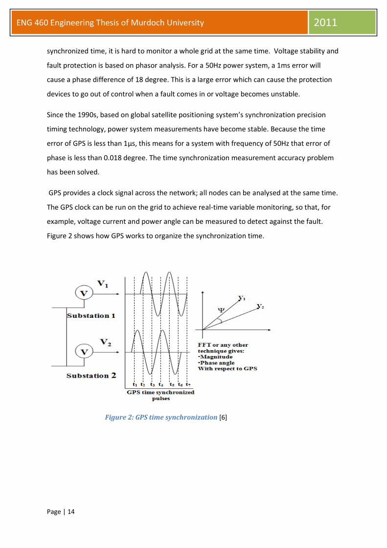
GPS provides a clock signal across the network; all nodes can be analysed at the same time.

The GPS clock can be run on the grid to achieve real-time variable monitoring, so that, for

example, voltage current and power angle can be measured to detect against the fault.

Figure 2 shows how GPS works to organize the synchronization time.

Figure 2: GPS time synchronization [6]

Page | 15


2.1.4 Hardware connection of synchronized phasor measurement devices

Figure 3: Phasor measurement unit block diagram [7]

Figure 3 above shows a simple diagram of the phasor measurement unit. The GPS receiver

provides one-pulse-per-second signal which connects to a phase-locked sampling clock. The

voltage and current inputs are in analog forms which go into an anti-aliasing filter. The filter

can be used to filter out input frequencies that are higher than the Nyquist rate. “As in many

relay designs one may use a high sampling rate (called oversampling) with corresponding

high cut-off frequency of the analog anti-aliasing filters. This step is then followed by a

digital ‘decimation filter’ which converts the sampled data to a lower sampling rate, thus

providing a ‘digital anti-aliasing filter’ concatenated with the analog anti-aliasing filters [7].”

The A/D converter is used to convert the analogue signal into a digital signal. The phasor

micro-processor calculates the phasor and uploads to the data concentrator. The GPS

receiver might be built into a phasor measurement unit or a substation. The sampling time

is a multiple of the nominal period. For a 50Hz system, the sampling frequency can be either

600Hz or 1200Hz. The output of the phasor measurement Unit is a positive sequence

voltage or current.

Figure 4 shows the basic diagram of a phasor measurement unit built in a two bus system.

Figure 4: Hardware connections of phasor measurement device in power system [8]

Page | 16


The input terminal of the phasor measurement unit usually connects to the secondary sides

of a three phase voltage transformer or a current transformer. The output from the phasor

measurement unit corresponds to voltage and current phasors. In the case shown in figure

4, the SEL device is a protective relay with synchrophasors built into them. The accuracy of

the GPS clock is ±500ns and the SEL offers±100ns accuracy [9].

The key features of the Phasor Measurement Unit (PMU):

Synchronicity: PMU device must be precisely synchronized with the clock signal as a

sampling basis. The synchronization error of the sampling pulse is less than 1us.

Speed: PMU measuring device must have high-speed internal data bus and external

communication interfaces to meet a large number of real-time data measurement,

storage, and send outs.

Precision: PMU measuring device must have a high enough accuracy. The signal

phase shift in PMU device measuring points must be compensated.

Large capacity: PMU measuring device must have enough storage capacity to ensure

long-term recording and saving of temporary data.

2.1.5 Report rate of Phasor measurement unit

Table1: required PMU reporting rates [5]

Table 1 above shows the required sampling period for a Phasor measurement unit

The reporting rate is the measurement period which is to be used when sampling the input

signals. Usually it is an integer numbers of times in one second. For example, if system

frequency is 50Hz, the period is 0.02s. The reporting rate of 10 is a sampling frequency of 10

times the system frequency. Therefore, the reporting period is 0.002s.

Page | 17


2.2 Applications of using synchrophasors

In the past 10 years, PMU-based wide area measurement technology has developed rapidly

and it has been applied in many aspects.

2.2.1 Monitoring the State Variables

Synchronized phasor measurement unit can provide voltage and current magnitude and

phase in real time. The state variables of a network analysis are based on these quantities,

especially the phase angle, as angles are used to determine the voltage stability and

operation margin.

.

Figure5: A single-line diagram presented for a network [4]

As consider in Figure 5. The real power flow from the sending end can be calculated by

] (Equation2-1)

The reactive power is expressed by

(Equation 2-2)

Recall the equation of voltage regulation which is defined as

(Equation 2-3)

The relationship between can be also written by the line impedance, the phase

angle and the reactive power supplied to the line. Therefore, from these three equations

above, the new equation of voltage regulation can be written as

(Equation 2-4)

Page | 18


If per unit measurements are used in the equation, so that the source voltage is 1 per unit,

then the equation will become

(Equation 2-5)

From equation 2-5, it can be seen that the receiving end voltage is only determined by the

angle between two buses as the line impedance and the reactive power are fixed

conditions. The verification and calibration of a network also depends on system

monitoring.

2.2.2 Fault recording and fault location

Figure6: SIMEAS R-PMU fault recorder [9]

Figure 6 is the SIMEAS R-PMU fault recorder with PMU technology installed on both sides of

the transmission line. These rewires have a number of functions that measure and

document the voltage and current phasors, power information, frequency recorder and

system diagnosis systems.

Figure7: PMU monitor a single-phase fault current [6]

Page | 19


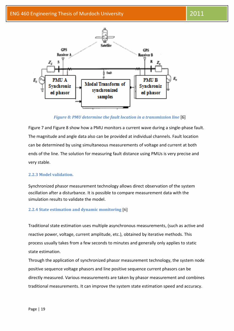
Figure 8: PMU determine the fault location in a transmission line [6]

Figure 7 and Figure 8 show how a PMU monitors a current wave during a single-phase fault.

The magnitude and angle data also can be provided at individual channels. Fault location

can be determined by using simultaneous measurements of voltage and current at both

ends of the line. The solution for measuring fault distance using PMUs is very precise and

very stable.

2.2.3 Model validation.

Synchronized phasor measurement technology allows direct observation of the system

oscillation after a disturbance. It is possible to compare measurement data with the

simulation results to validate the model.

2.2.4 State estimation and dynamic monitoring [6]

Traditional state estimation uses multiple asynchronous measurements, (such as active and

reactive power, voltage, current amplitude, etc.), obtained by iterative methods. This

process usually takes from a few seconds to minutes and generally only applies to static

state estimation.

Through the application of synchronized phasor measurement technology, the system node

positive sequence voltage phasors and line positive sequence current phasors can be

directly measured. Various measurements are taken by phasor measurement and combines

traditional measurements. It can improve the system state estimation speed and accuracy.

Page | 20


2.2.5 Wide area measurement principle and structure of the system

SCADA / EMS and related software applications represent scheduling control system. They

lack of accurate common time marks for recording data. This makes it is difficult analyse a

whole system dynamics analysis. However, as the GPS technology, modern communications

technology and digital signal processing technology develops ,wide-area power system

dynamic real-time monitoring becomes possible.[10]

Synchronized phasor measurement technique can improve equipment protection and

system protection. Based on PMUs, wide area protection systems can be designed.

A wide-area measurement system (WAMS) uses GPS to provide the synchronous clock for

wide-area power system state measurements. Wide area measurement systems will be

installed in all sub-stations with PMU synchronized phasor data underlying communication

network via high-speed data transmission to the control centre. The control centre can

evaluate these data in real time and dynamic monitoring to analyse network security and

stability.

A wide area measurement system structure includes a phasor measurement unit, system

master station and communications network. It directly measures the operating

parameters, such as phase angle, voltage and current. On the one hand it can monitor the

operational status of equipment, on-line fault diagnosis and protection and post-fault

analysis. On the other hand, through an efficient communication network, real-time

measurement data can be transmitted to the control centre, which monitors the

operational status of the whole network to predict the stability of the future.

2.2.6 System stability monitoring

Traditional power system testing method is focused on the detection of system stable

operation using a SCADA system. However, the traditional fault recorder can only record a

few seconds before and after the failure of the transient waveforms. But this large amount

of data, it is hard to save. SCADA provides about four seconds to update a steady-state data;

it cannot provide any help in predicting of the dynamic power, low frequency vibration or

fault analysis.

Phasor measurement unit can solve these problems.

Page | 21


It is very important to install synchronized phasor measurement units in power system

substations and power plants, building power system real-time dynamic monitoring system,

and through the dispatch center station, to enable power system monitoring and analysis of

dynamic processes, and enhance the stability of power system dynamic security monitoring.

Page | 22


Chapter 3 Method to obtain the synchronized phasor data

3.1 Introduction to the Discrete Fourier Transform (DFT)

3.1.1 Discrete Fourier Transform

Digital computers are usually used to analysis the phasor data of a power system. First, a

discrete-time signal is obtained by sampling the original analog waveform. A mathematic

method which is called Discrete Fourier Transform is then applied to this sampled data to

obtain a sampled frequency waveform.

Figure 9 shows a diagram of the sampled transform.

Figure 9: sample a waveform in discrete time

Consider periodic discrete-time finite signal, taking N samples from 0 to 2π, so that the

sampling time interval is 2π /N. The Fourier Transform can be expressed as [8]

(Equation3-1)

Where is the phasor of interest.

is the array of time domain data (the input signal

taken from N samples in one period)

X is the complex number to express phasor ( usually expressed in

rectangular form as a + bj)

N is the number of samples (usually is 12, 24, 36….)

A factor 2 usually appears in front of the sum as the signal with frequency ω

in the DFT has components at +ω and-ω. These components can be

combined and divided by the square root of 2 to get the RMS value.

In the Matlab simulation process, the k range from 1 to N, rather than 0 to

N-1.

Page | 23


The equation for the fundamental component can be rewritten as complex form as

following

(Equation 3-2)

Where

3.1.2 The Nyquist criterion

If a signal contains frequency components greater than Hz, then sampling the signal at

cannot express the signal, an artefact called aliasing takes place. Therefore, any analog

signal must be bandwidth limited [2].

3.2 Matlab program for obtaining the phasor expression (DFT method)

3.2.1 Using Matlab to sample a pure sine-wave to obtain its magnitude and angle

In the following simple case, a Matlab programme is used to sample a known sine wave to

verify its magnitude and angle.

The input signal is given by

The numbers of sampling points in one period are 12, so that sampling frequency is

12*50=600Hz.

3.2.2 Data recursion process

As the measurement and calculation is a continuous process, updating the calculation

should be reconsidered when the new measurements comes in. For example, if we take 12

points in 1 period and for some reason the measurements stop or we want to consider a

new measurement point, it is not necessary to start from the initial sample point 1. There is

a method, which is called ‘recursive algorithm’ that can update the sampled calculations.

The general form of the equation is given by [8]

+

- )* (Equation 3-3)

Page | 24


3.2.3 Input data at off-nominal frequency

If the sampling rate is based on the nominal frequency, then the instantaneous phase angle

and magnitude will vary with time when the input signal has an off-nominal fundamental

frequency.

For example, in the case given in section 3.2.1, if the frequency of the input signal is 51Hz

(which may happen in a real situation when load demand changes), errors will occur

between the accuracy value, and the measurement value and the result will be incorrect to

use in predicting power stability or other applications.

Equation below is the formula to calculate the sample of single frequency components. [3]

(Equation 3-4)

is the actual frequency of the wave form

is the nominal frequency of sampling measurement device

The equation for estimating the phasor at the off-nominal frequency will become

(Equation 3-5)

Here [3], A =

B=

It can be seen that the values of A and B do not only depend on the off-nominal frequency,

but depend on the number of samples in one cycle. Figures 10, 11 below show A and B

factors as a function of frequency.

Table 2 shows the A and B values, magnitude and angle errors at 24 samples per period,

with a nominal frequency of 50Hz, keeping the magnitude of the signal of 220-volt

magnitude voltage and a phase angle at π/5.

Page | 25


Figure 10: A factor as a function of frequency

Figure 11: B factor as a function of frequency

From the two figures above, it can be seen that the A value is close to 1 and B approaches

0, the phasor estimates by DFT equals to the true phasor value at the nominal frequency.

0.982

0.984

0.986

0.988

0.99

0.992

0.994

0.996

0.998

1

45 46 47 48 49 50 51 52 53 54 55

Mag

nit

ud

e

Hz

A factor as a function of frequency

-0.06

-0.05

-0.04

-0.03

-0.02

-0.01

0

0.01

0.02

0.03

0.04

0.05

0.06

45 46 47 48 49 50 51 52 53 54 55

Mag

nit

ud

e

Hz

B factor as a function of frequency

Page | 26


Table2: error of off-nominal frequency measured at a nominal frequency of 50Hz and

sampling frequency 1200Hz

Freq(Hz) A B magnitude angle Mag error Angle error Mag error%

Angle error%

55 0.98366 0.047435 219.8488 33.4125 0.1512 2.5875 7.1875% 0.0687%

54.5 0.986752 0.043025 220.1848 33.6569 0.1848 2.3431 6.5086% 0.0840%

54 0.989524 0.038532 220.4537 33.9042 0.4537 2.0958 5.8217% 0.2062%

53.5 0.991973 0.033959 220.6494 34.1547 0.6494 1.8453 5.1258% 0.2952%

53 0.994099 0.029308 220.7726 34.4084 0.7726 1.5916 4.4211% 0.3512%

52.5 0.9959 0.024584 220.823 34.6653 0.823 1.3347 3.7075% 0.3741%

52 0.997375 0.019791 220.801 34.9254 0.801 1.0746 2.9850% 0.3641%

51.5 0.998523 0.014932 220.707 35.1889 0.707 0.8111 2.2531% 0.3214%

51 0.999343 0.010011 220.5411 35.4558 0.5411 0.5442 1.5117% 0.2460%

50.5 0.999836 0.005032 220.3039 35.7262 0.3039 0.2738 0.7606% 0.1381%

50 1 0 220 36 0 0 0.0000% 0.0000%

49.5 0.999836 -0.00508 219.6165 36.2773 0.3835 0.2773 0.7703% 0.1743%

49 0.999343 -0.01021 219.1669 36.5585 0.8331 0.5585 1.5514% 0.3787%

48.5 0.998523 -0.01538 218.6479 36.8433 1.3521 0.8433 2.3425% 0.6146%

48 0.997375 -0.02058 218.0602 37.1315 1.9398 1.1315 3.1431% 0.8817%

47.5 0.9959 -0.02582 217.4037 37.4239 2.5963 1.4239 3.9553% 1.1801%

47 0.994099 -0.03108 216.6797 37.7198 3.3203 1.7198 4.7772% 1.5092%

46.5 0.991973 -0.03636 215.8886 38.0194 4.1114 2.0194 5.6094% 1.8688%

46 0.989524 -0.04167 215.0307 38.3237 4.9693 2.3237 6.4547% 2.2588%

45.5 0.986752 -0.04698 214.1077 38.6313 5.8923 2.6313 7.3092% 2.6783%

45 0.98366 -0.05231 213.1195 38.9437 6.8805 2.9437 8.1769% 3.1275%

From Table 2 above, it can be seen that the off-nominal frequency is greater than 50Hz , the

phase angle decreases and the magnitude of the phasor increases. When the off-nominal

frequency is less than 50Hz, the phase angle increases and the magnitude of the phasor

decreases. The angle error at off-nominal frequency is quite small compared with the

magnitude error. In fact, the frequency will vary along with load and generation changes. If

the load demands exceed supply, the grid frequency falls and if there is too much

generation, the grid frequency will rise. However, normally the grid frequency is operated at

(50 [11]. Therefore, for a 220V voltage system, the maximum

error in magnitude is only 0.4 V (at 49.5Hz) by using PMU measurement device and the

maximum angle error is in 0.3835degree (at49.5Hz). The PMU is a good method for

monitoring the voltage and current, and the data is quite credible. Figure 12 and Figure 13

give the error in percentage between the actual phasor and the measurements values.

Page | 27


Figure 12: %error at actual angle at off-nominal frequency using nominal clock

Figure13: % magnitude error at off-nominal frequency using nominal clock measurement

0

0.01

0.02

0.03

0.04

0.05

0.06

0.07

0.08

0.09

45 45.5 46 46.5 47 47.5 48 48.5 49 49.5 50 50.5 51 51.5 52 52.5 53 53.5 54 54.5 55

%e

rro

r

Hz

% error between actual angle and measurents

0.0000% 0.2500% 0.5000% 0.7500% 1.0000% 1.2500% 1.5000% 1.7500% 2.0000% 2.2500% 2.5000% 2.7500% 3.0000% 3.2500% 3.5000%

45 46 47 48 49 50 51 52 53 54 55

%e

rro

r

Hz

% magnitude error at off-nominal frequency using nominal clock measurement

Page | 28


Table 3 below shows that the sampling rate affects the values of A and B

Sample points A B Magnitude(V) angle(degree)

12 0.99853 0.015475 220.7462 35.1596

24 0.998523 0.014932 220.707 35.1889

36 0.099852 0.014834 220.707 35.1942

48 0.099851 0.0148 220.6983 35.1961

72 0.099521 0.014776 220.6966 35.1974

84 0.099852 0.014771 220.697 35.1976

96 0.099852 0.014767 220.696 35.1968

Table3: magnitude and angle sampling at different points

It can be seen that changing the sampling frequency has little effect on the calculated

values.

3.2.4 Input signal with noise

There are two simple methods for estimating a phasor with noise [12]

In a real situation, noise affects the accuracy of the measurements. This section introduces

methods for correcting data with noise present.

Consider a pure voltage waveform which is given by

and has a phasor of its form ∠ .

We can take samples from a period to estimate the unknowns of magnitude and phase as in

case 1; however, this time only 2 samples will be considered.

The expression of voltage at time t1 and t2 are given by

(Equation 3-6)

(Equation 3-7)

These equations can be written in matrix form, using

to simplify it.

= (Equation 3-8)

Page | 29


= ) (Equation 3-9)

The matrix form is [

(Equation

3-10)

Solving the equation and it gives:

(Equation 3-11)

(Equation 3-12)

From the solution of and , both the magnitude and the angle can be

estimated by

= (Equation 3-13)

And

In the more general form,

(Equation 3-14)

(Equation 3-15)

is the interval length between two samples.

Recall case 1

f =50Hz

In above process, a mean value of 0 and standard derivation 1 noise was added to the

signal. The answer from the two point method is magnitude 220.5673 with angle 36.082

degree. The noise generated in Matlab is a random number. The value of a random number

can vary from one simulation to the next. However, as the mean and standard derivation is

fixed. The difference in each period simulation will be small.

Page | 30


3.2.5 Accuracy of the DFT method

The Discrete Fourier Transform method is one of the most widely used method in

mathematical modelling. In essence, it breaks down a periodic function into a series of

orthogonal functions (such as sin and cos functions). The Fourier transform is a

transformation in the whole time domain, and it is truncated by the DFT. This cause an

artifact called leakage. As the power system frequency is always changing, there is no way

to do each cycle as just an integer multiple of the sampling frequency. Therefore, the input

signal must be band limited and the sampling rate must very high.

3.2.6 Total Vector Error (TVE)

The term Total Vector Error is the accuracy level of the synchronized measurements over a

range of continuous operation under steady-state conditions. As with other equipment, the

accuracy of a PMU is given by the manufacturer according to the amount of measured

signals which include amplitude, phase angle and frequency. IEEE standard gives a definition

of Total Vector Error which provides the accuracy of PMU in a variety of measurements

within a range of overall error.

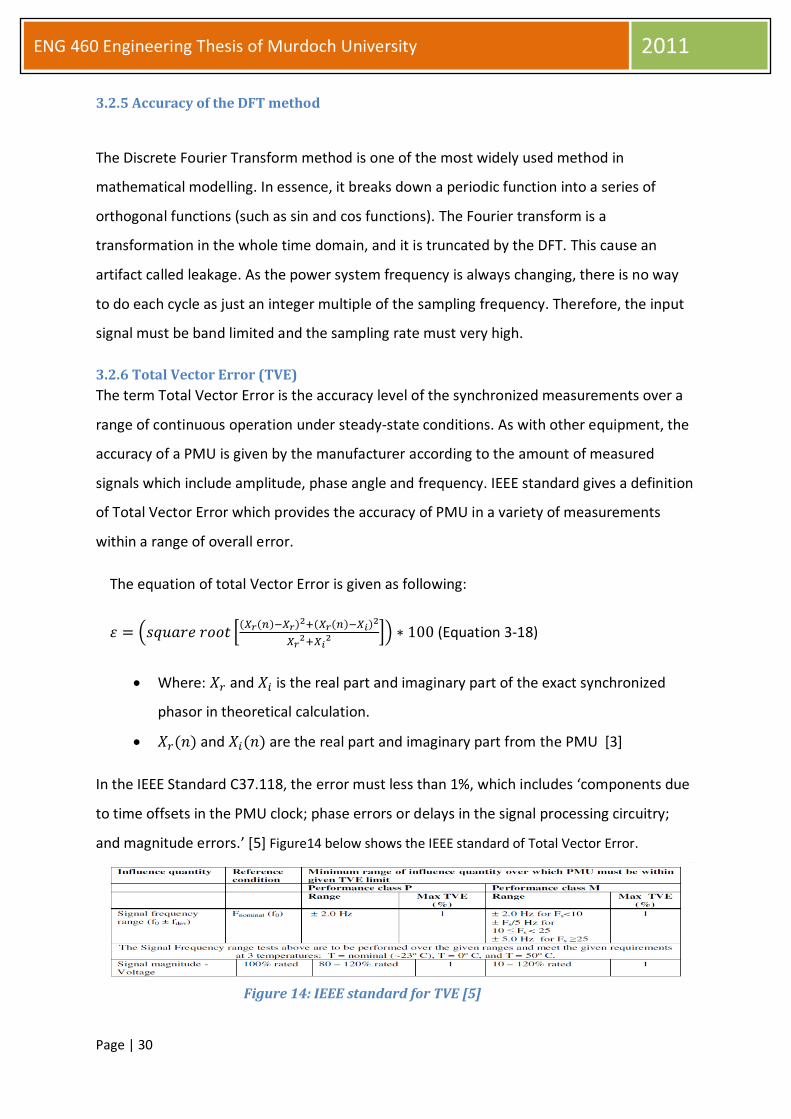
The equation of total Vector Error is given as following:

(Equation 3-18)

Where: and is the real part and imaginary part of the exact synchronized

phasor in theoretical calculation.

and are the real part and imaginary part from the PMU [3]

In the IEEE Standard C37.118, the error must less than 1%, which includes ‘components due

to time offsets in the PMU clock; phase errors or delays in the signal processing circuitry;

and magnitude errors.’ [5] Figure14 below shows the IEEE standard of Total Vector Error.

Figure 14: IEEE standard for TVE [5]

Page | 31


Chapter 4 Using Synchronized phasors to predict power stability and

transmission line parameter and fault location analysis

4.1 Method of considering voltage stability index

A number of research has been done on simultaneous measurements of voltage stability

and voltage stability index analysis in recent years. There are many methods to predict the

power stability, such as Power Voltage or Reactive Power Voltage methods and Jacobian

matrix method [13]. In future years use of synchronized phasor measurement technology

for real-time monitoring of power system voltage stability will be the inevitable trend of

development. Voltage stability index analysis is an analytical method that assesses voltage

stability.

4.1.1 Concept of voltage stability

If a system maintains a load voltage to ensure that the load admittance is increased, load

power consumption will also increase while the power and voltage are controllable. It is

called voltage stability; otherwise it is called voltage instability.

Consider a simplified power system model as shown in Figure 15

Figure 15: A simple two bus power system to determine the Voltage stability index [4]

Current flows from the sending terminal to the receiving terminal. It can be expressed in

two forms which are the relationship between sending end power and voltage and the

relationship between receiving end power and voltage. Use Vs to express the sending end

voltage, and Ps and Qs to express the sending end active power and reactive power

respectively. Use Vr to express the receiving end voltage, and Pr and Qr to express the

Page | 32


receiving end active power and reactive power respectively. The current flowing through

the transmission line can be expressed in two equations which can be built as followings:

(Equation 4-1)

=

(Equation4- 2)

When power flows through the transmission line, losses occur. The power losses can be

considered as equation 4-3 and equation4- 4 below.

(Equation4- 3)

(Equation 4-4)

Here, R and X are the resistance and reactance of the transmission line.

By combining the equations (Equation 4-1 to Equation 4-4), a much more complicated

equation for can be obtained [14]:

+

= 0 (Equation 4-5)

If the equation4- 5 has real root solutions, 2- 4

should be greater than 0.

The final answer [14] is L = 4[ -

≤1 (Equation4-6)

is the voltage angle difference between the two buses.

L is defined as the voltage stability index

Equation4- 6 indicates when L less than 1, the system remains stable. Otherwise, the system

will be unstable.

4.2 Online parameters method using synchronized phasor

In the past, to determine the positive sequence impedance of a line usually requires placing

a three-phase short circuit at the end of the line and adding a three-phase power supply to

the beginning of the line. The measurements were focused on three-phase current, voltage

and power values, and then in accordance with measured values the line parameters could

Page | 33


be calculated. This method is too complicated. However, with the availability of

synchronized phasor measurements, this problem can be solved.

The new method to determine parameters is based on the distributed line model for the

transmission line. It assumes that the voltage and current at each end of the line are

provided by the synchronized phasor measurement device. The exact solution of the line

characteristic impedance, propagation constant, inductance and capacitance can be

calculated by equations with voltage and current phasors.

4.2.1 Two-port network

A two-port network is an electrical circuit which can be used in a power system to find the

characteristic parameters. The model of the two-port network can be seen in Figure 16

below.

Figure 16: two-port network model

4.2.2 Pi model of the transmission line

The two-port network can also represent a transmission line model. Figure 17 shows the

long transmission line model, which is accurate longer than 250km.

Figure 17: pi type of transmission line [15]

Assume that the two-port network voltages and currents at both terminals are known. The

relationship between voltage and current can be expressed as:

Page | 34


(Equation4-7)

where A =

; B =

( at ); C = -

( at D = -

(at )

For the long transmission line, the shunt admittance will be included in the model. The

shunt admittance can be defined as

(Equation4-8)

The unit of Y is given in unit S/km; the capacitance is usually given as a susceptance B = ;

From Equation 4-7 and Figure 17, the two –port network to express the transmission line

parameters becomes:

(Equation 4-9)

By rewriting this equation, expression for Z and Y can be obtained as

Z = ( –

; Y/2 = ( (Equation 4-10)

When a power system is operating, the frequency will be a little different as the load

changes. Therefore the transmission line parameters are also changing as the load,

frequency and environment changes. The actual parameter values will be different from

offline measurements. Those parameters are the foundation component of a reliable power

system model, which can be used in state estimation, power flow, stability analysis and the

protective relay calculations. Assuming the synchronized phasor data is given, the algorithm

for online estimation of distribution line parameters can be implemented. A comparison

also can be done between the measured values and the manufacturer’s values. Therefore, a

statistical analysis can be done to predict parameter behaviours.

Page | 35


4.3 Fault location in Transmission lines using synchronized phasor

4.3.1 Method for short transmission line model

Figure 18 shows a short transmission line model. The relationship between the sending end

and receiving end can be given by the equation.

= + * * (Equation 4-11)

is the transmission line impedance per km and is the length of the line

Figure 18: short transmission line model

Consider a fault that occurs in the transmission line and x km from . Let the fault point

voltage given as , the current to the left side of the fault point as and the current to the

right side of the point as . The new relationship between source voltage and load voltage

can be written by two equations as follows.

* (Equation 4-12)

* + (Equation 4-13)

are the source voltage and load voltage when a fault occurs.

From the two equations, a new equation for finding the fault location can be written as

(Equation 4-14)

I f we know the source and load voltages, and the currents at the left side and right side of

the points; we can determine the fault location.

Page | 36


4.3.2 Method for π type model

Figure 19: π type line model [15]

As the distance of the line increases, the short line model cannot be used. A π type line

model can be used instead. The π type line model is given in Figure 19. The relationship

between source voltage and load voltage is given by the following equation:

+ (Equation 4-15)

where A = (1+YZ/2) and B=Z (See Equation 4-9)

Consider a fault that occurs in the transmission line x km from . Let the fault point voltage

be and the current at the left side of fault point be and current at the right side of the

point be . The new relationship between source voltage and load voltage can be written

by two equations as follows.

(Equation 4-16)

* +

(Equation 4-17)

We can simplify the equation as

) = ( * +

(Equation

4-18) I f we know the source and load voltages and the currents at the left side and right

side of the points, we can determine the fault location.

Page | 37


4.3.3 Method for long line distributed model

For a large power system with long transmission and distribution lines, the short line model

and pi model are not accurate enough to represent the line. A good way to represent the

line is by separating the line into small-length segments as shown in figure 20 below.

Figure 20: long transmission line model [15]

The equation of the transmission line is also given in lecture notes as A B C D parameters.

(Equation 4-19)

(Equation 4-20)

Here are the sending voltage and current;

are the receiving end voltage and current;

= m-1 is the propagation constant of the line and is the characteristic of the

line.

Consider a simple system as above. Assume the phasor measurement units were

installed in the sending end and receiving end of the circuit.

First, write the equations of the transmission line in matrix form, assuming that the fault

happens at some point along the transmission line. Take and as the reference point

voltage and current before fault occurs.

Assume the system is balanced, so that a one-line diagram can be used to represent the

three phase system. The distance of the line is L.

Page | 38


=

(Equation 4-21)

Take the inverse of the transmission line matrix:

Inverse matrix =

Both sides multiply by the inverse matrix, Equation 4.21 can be rewritten as

(Equation 4-22)

There is

(Equation 4-23) and

(Equation 4-24)

Alternatively, we can write a line parameter equation from the receiving end to the fault

point. The process will be same as above.

(Equation 4-25)

(Equation 4-26)

-

(Equation 4-27)

From Equations 4-22 to 4-27, we get another two equations and parameter can be

calculated.

The two equations are

(

*

(Equation 4-28)

(

= *

(Equation 4-29)

Page | 39


From which

and

When the fault occurs anywhere in the transmission line, the fault point voltage and current

can be represented by sending end and receiving end voltage and current as the following

equations

(Equation 4-30)

(Equation 4-31)

From these two equations above, the fault location x can be calculated as a complicated

form.

However, it is hard to build a system with a long transmission line model in ICAP. It can be

carried out on other software tools rather than ICAP. From equations above, it can be seen

that long transmission line fault location determination can be done without knowing the

parameters of the transmission line.

4.4 Testing a simple system

4.4.1 Test case with a pure input signal

Matlab software can be used to simulate the power flow of a power system. Typically, under

the normal operating conditions, power will be excited supplied using a sinusoidal voltage

waveform with a 50Hz or 60Hz frequency from synchronized generators. If a three-phase

system is balanced, a single-line diagram can be used to simplify the system by just

analysing one phase. Consider a simple two-bus system which concerns one generator, one

transmission line and one load. The generator can be modelled as a sinusoidal waveform in

sampling time. The transmission line can be modelled as impedance (resistance and

reactance). If the parameters of the transmission line and load and generator are already

known, the problem will be to solve a first order differential equation based on Kirchoff’s

Voltage and Current laws. If the circuit includes capacitors, the equation will become a

Page | 40


second-order or higher. Phasor analysis can be carried out using hand calculations to check

the software solution.

Consider the example given in Figure 21:

Figure 21: signal line diagram in test

The generator voltage is a 2400 V (RMS) at 50Hz sinusoid with a zero phase angle, so it acts

as the reference phase.

The values of inductances can be specified by their reactance values. The transmission line is

modelled by a pure inductance to simplify the calculations. The transmission line impedance

is j2.0Ω and the load impedance is given by 16Ω+12.57jΩ

From the kirchoff’s Voltage Law:

(Equation 4-32)

Putting values into the equation:

=

= 110.9∠-42.33 A

As we are interested in the behaviour of the transmission line, the load voltage and the

generator voltage need to be known. The load voltage can be calculated as

=

Page | 41


= 110.9∠-42.33*(16+12.57j) =2256.6∠-4.17V.

Use the method of Voltage stability index to verify the stability of the system.

Recall the equation L = 4[ -

L=4*[2400*2256.6*cos(-4.17) – 2256*2256*cos2(-4.17)]/(2400)2 =0.2343≤1

Therefore the system is stable as the voltage stability index value is much less than 1.

Now we use synchronized phasor theory to verify the answer of the magnitude and angle of

the source and load voltages. Figure 22 shows the simulink diagram and results from

Matlab. The sample time is 0.1ms and the sample period is 0.04s. The generator is modelled

as a digital clock box which connects to a function box. The function box is the sinusoid

wave with time tag from a digital clock input. The data can be taken from the Matlab

workspace. The transmission line and load can be modelled as du/dt. The simulation system

is given in Figure 22 and the results in figure 23-figure-figure24.

The data will be taken when the system reaches steady-state.

The simulation solution gives Vs=2400V, Angle=-36 degree and Vr=2253.5V, Angle=-39.5645

degree. The calculated generator voltage angle is -36degree rather than 0 this because the

start sampling point does not at the peak of the input wavefrom.

From the DFT calculation, it can be seen the answer is very close to the hand calculation.

Figure 22: two bus system simulations in Matlab

Page | 42


Figure 23: load current performance

Figure 24: source voltage and load voltage

4.4.2 Test Case in pure input signal with noise

The noise can be simulated at sample time 0.001s with a mean zero and variance 0.02% of

the magnitude. Figure below shows the circuit diagram in Simulink , the noise can be

expressed as random numbers . The diagram can be seen in Figure 25 below. The results are

given in Table 4.

Page | 43


Figure 25: two bus system simulation with noise

Figure 26: load voltage and source voltage

Measurement number

Generator voltage in Volt

phase angle(degree)

Load voltage in Volt

Phase angle (degree)

Angle difference in degree

1 2400 -35.9793 2253.6 -39.5438 3.5645

2 2401 -35.9928 2254.5 -39.5574 3.5646

3 2399.7 -35.9963 2253.2 -39.5605 3.5642

4 2399.1 -35.9994 2252.7 -39.5593 3.56

5 2400 -35.9908 2253.6 -39.5553 3.5645

Theoretical result

2400 0 2256 -4.17 4.17

Table 4: Results of 5 measurements at nominal frequency with noise

Page | 44


Also the error between theoretical value and measurement value can be seen in table 5

below.

Measurement number


Difference in Volt


Difference in Volt

1 2400 0 2253.6 2.4

2 2401 1 2254.5 1.5

3 2399.7 0.3 2253.2 2.8

4 2399.1 0.9 2252.7 3.3

5 2400 0 2253.6 2.4

Theoretical result

2400 0 2256 0

Table5 error of magnitude compare with the theoretical results

Voltage magnitude and angle at noise condition is only little different as the theoretical

result. The reason might be that the noise which is added into the system is quite small.

However, the answer shows using synchronized phasor data calculation closely enough

to the theoretical calculation.

4.4.3 Test system with off-nominal frequency

In reality, the frequency of the generator will be changed as the load changes or

disturbances occur. However, the changing of frequency will be smooth.

The expression of the generator’s frequency in Matlab can be given by

= 2400* (2*π*(50+ (2*π*9*t))*t)

(2*π*9*t) is the variable part of the frequency.

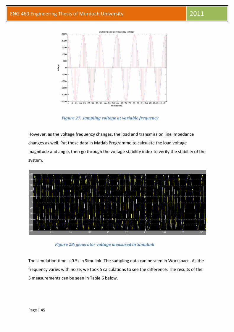
Figure 27 below shows the diagram of the voltage in nearly one period. The sample data is

taken every 0.0001 second. Figure 28 is the voltage diagram which is observed in Matlab

scope.

Page | 45


Figure 27: sampling voltage at variable frequency

However, as the voltage frequency changes, the load and transmission line impedance

changes as well. Put those data in Matlab Programme to calculate the load voltage

magnitude and angle, then go through the voltage stability index to verify the stability of the

system.

Figure 28: generator voltage measured in Simulink

The simulation time is 0.5s in Simulink. The sampling data can be seen in Workspace. As the

frequency varies with noise, we took 5 calculations to see the difference. The results of the

5 measurements can be seen in Table 6 below.

1 6 11 16 21 26 31 36 41 46 51 56 61 66 71 76 81 86 91 96 101106111116-2500

-2000

-1500

-1000

-500

0

500

1000

1500

2000

2500

millsecond

vola

tge

sampling varible frequency volatge

Page | 46


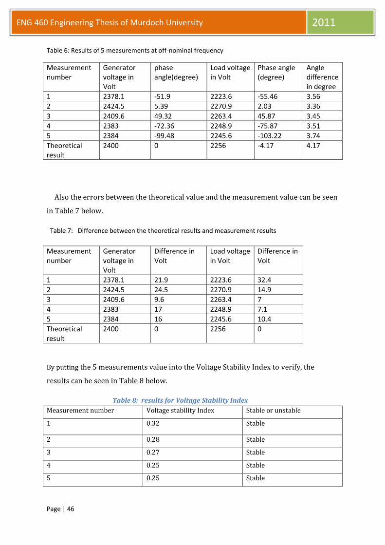
Table 6: Results of 5 measurements at off-nominal frequency

Measurement number


phase angle(degree)


Phase angle (degree)

Angle difference in degree

1 2378.1 -51.9 2223.6 -55.46 3.56

2 2424.5 5.39 2270.9 2.03 3.36

3 2409.6 49.32 2263.4 45.87 3.45

4 2383 -72.36 2248.9 -75.87 3.51

5 2384 -99.48 2245.6 -103.22 3.74

Theoretical result

2400 0 2256 -4.17 4.17

Also the errors between the theoretical value and the measurement value can be seen

in Table 7 below.

Table 7: Difference between the theoretical results and measurement results

Measurement number


Difference in Volt


Difference in Volt

1 2378.1 21.9 2223.6 32.4

2 2424.5 24.5 2270.9 14.9

3 2409.6 9.6 2263.4 7

4 2383 17 2248.9 7.1

5 2384 16 2245.6 10.4

Theoretical result

2400 0 2256 0

By putting the 5 measurements value into the Voltage Stability Index to verify, the

results can be seen in Table 8 below.

Table 8: results for Voltage Stability Index

Measurement number Voltage stability Index Stable or unstable

1 0.32 Stable

2 0.28 Stable

3 0.27 Stable

4 0.25 Stable

5 0.25 Stable

Page | 47


From the calculation of Voltage Stability Index, it can be seen that the system is still

stable even when operated at off-nominal frequency with noise. Figure 29 shows the

source voltage and load voltage which is observed using the Matlab scope.

Figure29: source voltage and load voltage

4.4.4 Test the fault behaviour of a two bus system

Figure 30: Fault condition simulation in ICAP

Page | 48


Figure 30 above is the same system as used in Section 4.4.1. Now we want to capture the

circuit behaviour when a fault occurs. Also, after the fault is cleared, we want to observe the

new steady-state magnitude and angle value at the generator and the load. A switch can be

added after the transmission line, which simulates a fault on the load side. The short circuit

can be modelled by a switch which is controlled by a pulse. The pulse is generated at 0.06s

to 0.4s. Therefore, at that time, the switch will close and current will flow through the

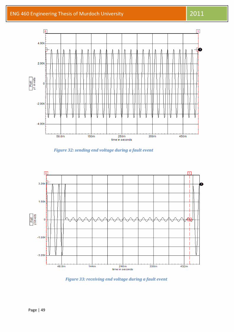
switch to the ground. After 0.4s, switch will open and the fault will be cleared. Figures 31,

32, 33 show voltage and current diagrams in the interval 0 to 0.5s.The output data will be

exported from ICAP to Matlab to be calculated at phasor form.

Figure 31: system current diagram during a fault event

From Figure 31, it can be seen that the current increases dramatically at 60ms when the

fault is initial. When the fault is cleared, the magnitude of current is almost the same as

before the fault. Figure 34 and figure 35 are the source voltage and load voltage which were

observed using ICAP scope.

Page | 49


Figure 32: sending end voltage during a fault event

Figure 33: receiving end voltage during a fault event

Page | 50


Table 9 gives the results of generator voltage and load voltage at 3 stages which are before

the fault occurs; during the fault occurs and after the fault occurs.

Conditions Generator voltage(Volt RMS)

Angle (degree)

Load Voltage(Volt RMS)

Angle (degree)

Difference (degree)

Before fault 2393.2 -36 2250.7 -40.17 -4.17

During fault 2393.2 -36 118.83 -122.98 -86.98

After fault 2393.2 -36 2247.5 -40.26 -4.26

Table 9: circuit response during a three balance fault

The generator voltage angle is -36 degree rather than 0 degree; because we take the first

account point at 1 .The phase shift is 360degree /10 =36 degree. However, we are only

interested in the angle difference between generator and the load in steady-state rather

than individual angles.

Recall from the hand calculations =2400V, =2256.6V and δ = -4.17 degree.

The difference between the theory and the simulated results is less than 10V.

4.4.5 Test π type transmission line parameters

Figure 34: sampling transmission line in ICAP

The diagram above is shown a test case in ICAP software. The equivalent π network

parameters are given as follows:

Page | 51


Z =88.31i and Y=6.079e-4i. These values are converted to inductance and capacitance at the

nominal frequency of 50Hz. The value for inductance and capacitance are 0.2811H and

1.935uH.

The voltage source is a 200kV (RMS) 50Hz sinusoid and the load is modelled as

40Ω+0.4456jΩ.

This system is modelled in ICAP simulated in Transient Analysis is carried out with Data Step

Time 2 ms and total Analysis Time 5s.

Data can be exported to a Matlab m file and edited. Samples were taken over 1 period of

the waveform; 10 data points were taken and a short Matlab programme can be used to get

the synchronized phasor voltage and current.

This test was done by setting four different conditions. The first condition is setting source

voltage frequency at 50Hz. The second and third conditions are setting source voltage

frequency as 50.5Hz and 49.5Hz.The last condition is setting the load as a pure resistance

load. The results can be seen in table 10 below.

Load type Source

frequency

Value for Z Value for Y Difference for

Z from

theoretical

Difference

for Y from

theoretical

Resistance and

Inductance

50Hz -0.8254+89.22i 6.32e-4i 1.035% 4%

Resistance and

Inductance

50.5Hz -1.57+91.3811i 6.3239e-4i 3.5% 4.03%

Resistance and

Inductance

49.5Hz -0.048+87.1523i 6.3079e-4i 1.31% 3.77%

Resistance 50Hz -1.2153+89.6943i 6.3143e-4i 1.58% 3.87%

Theoretical 50Hz 88.31i 6.079e-4i 0 0

Table 10: Results of Z and Y parameters from Matlab

It can be seen from simulation results that the values of Z and Y will increase as the system

frequency increases when the load type is fixed.

Page | 52


4.4.5 Test fault location in short line model

Recall equation

We can use ICAP program to verify this equation. Figure below shows a circuit which

presents the fault occurring in the middle of the transmission line. The result will be in

complex form, we only consider the real part as the location. Assume that the fault is a

three phase balanced fault. Therefore, a single line diagram can represent the fault

condition. In fact, the length of a short transmission line should be less than 80km according

to lecture notes. However, to simplify the calculation we just assume the length of the line is

200km long and a pure inductance line.

Figure35: diagram for determine fault location

Specifications for this circuit are as follows:

= Volt

= 16+12.57j Ω

Figure 38 shows simulation results. From top to bottom are load voltage, source voltage,

source current and load current. The data can be obtained at ‘Edit test file’. Using Matlab

program, the DFT method is used to calculate location

Page | 53


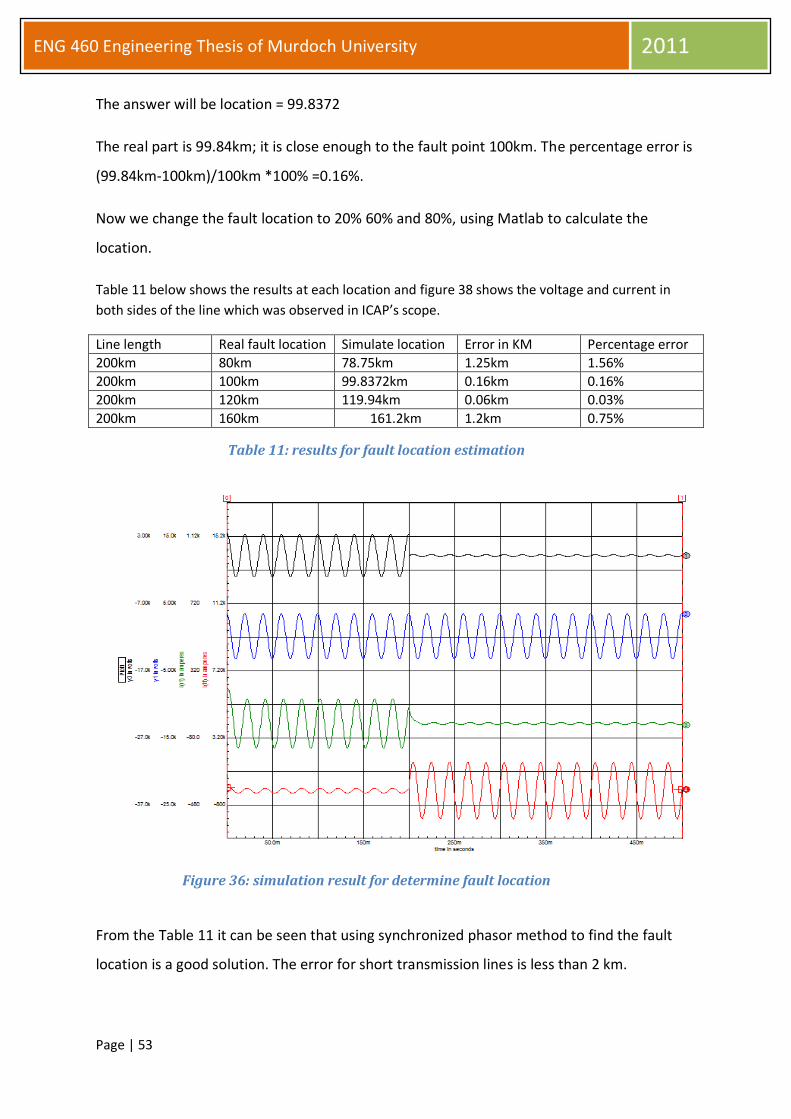
The answer will be location = 99.8372

The real part is 99.84km; it is close enough to the fault point 100km. The percentage error is

(99.84km-100km)/100km *100% =0.16%.

Now we change the fault location to 20% 60% and 80%, using Matlab to calculate the

location.

Table 11 below shows the results at each location and figure 38 shows the voltage and current in

both sides of the line which was observed in ICAP’s scope.

Line length Real fault location Simulate location Error in KM Percentage error

200km 80km 78.75km 1.25km 1.56%

200km 100km 99.8372km 0.16km 0.16%

200km 120km 119.94km 0.06km 0.03%

200km 160km 161.2km 1.2km 0.75%

Table 11: results for fault location estimation

Figure 36: simulation result for determine fault location

From the Table 11 it can be seen that using synchronized phasor method to find the fault

location is a good solution. The error for short transmission lines is less than 2 km.

Page | 54


Chapter 5 Conclusion and further studies

5.1 Summary of this thesis

Phasor measurement unit are new technologies that have developed rapidly in the past

decades. The core technology is based on GPS, and provides real time measures of the

voltage and current in phasor form. This thesis uses DFT theory to sample the voltage and

current in real time. ICAP and Matlab software are used to simulate the input waveform in

discrete time. Therefore, all the calculated data are synchronized. The off-nominal

frequency with noise and the error in using the DFT are also included in the simulation. The

results are quite good, as expected. These simulations take a two bus system as an example

and present the methods in detail for voltage stability analysis, transmission line parameters

calculation and fault location determination. The voltage stability index method is quite

simple compared with other methods. It just requires the voltage at each bus, without

knowing other information. The method for determining transmission line parameters is

quite reliable, for a pi type transmission line the maximum error is only 4% at nominal

frequency and 4.03% at off-nominal frequency. The algorithm simulation of fault location,

detect in proved to be quite efficient and accurate. The maximum error for a short line

model is only 1.3%. It is not necessary to know the parameters of the transmission line in

the long line model. The A and B factors are also important information which can be used

to adjust the accuracy result at off-nominal frequencies.

5.2 Problem in simulations compared with real world measurements

Simulation is one of the useful methods to predict power system properties. However,

simulation cannot solve all of the problems in a real power system. The real condition will

be more complicated than examples given in simulators. There are many factors that

influence a system. One line diagram has been used in this thesis to present a three phase

balance system. In the real world, the system can be unbalance and the noise might have a

mean value.

Page | 55


5.3 Further study in this area

The fault conditions in investigated in this thesis only assume a three phase balance fault. In

the real world, fault types can be three phase balance fault, line-to-line fault, single line-to-

ground fault and double line-to-ground fault etc. Different types in ICAP have been

simulated. However, it is difficult to build the model and get the correct result. Many studies

in fault location determination can be estimated by other software rather than ICAP and

Simulink. Some simulations predicting voltage stability is built in Power World. Power World

is an easy way to build a more complicated system rather than Matlab. However, in Power

World the frequency is fixed and it is difficult to model noise. The data can be exactly

synchronized. In a future study, the project should focus on a large systems voltage stability

algorithm. The protection relays and transformers to tap control also need to be considered.

In predicting the fault location, the project should focus on the different types of faults, and

estimate the method for the situation where only one bus has an installed phase

measurement unit.

5.4 Summary of Phasor Measurement units

PMUs can measure magnitudes and phase angles on each node voltage with high-speed

communication to transfer data to the control centre. If in the whole network all the buses

are equipped with PMUs, the whole system of node voltages and currents could be

observed without any iterative calculation. If each power plant and substation is equipped

with a PMU, the information in dynamic response will be collected in a uniform time

standard and the whole system dynamics can be observed. However, due to the high price,

PMU installation in a whole power plant is unrealistic. How to optimize the PMU location in

a power substation is further work that needs to be investigated.

A synchronized phasor measurement device-based wide area measurement system

provides for new security monitoring which has been used in dynamic state estimation,

stability, prediction and control, model validation, relay protection and fault location.

Therefore, we should develop as soon as possible synchronized phasor measurement

devices or systems to meet these requirements.

Page | 56


Appendix

(1) Matlab code in 3.2.1 DFT method obtain magnitude and angle of pure sinusoid wave

clear for k=1:12; y(k)=220*cos(2*pi*(k/12)+pi/5)%sampling data in one period 12 points r(k)=cos(k*(pi/6))-sin(k*(pi/6))*j%cos(ka)-sin(ka)j; Ymatrix =y' % r is [1*8] change y to [8*1] matrix F=(2/12)*r*Ymatrix; % 2 instead of sqrt(2) is magnitude Magnitude = abs(F) Angle=angle(F)*180/pi end

(2) Matlab code in 3.2.5 Estimation phsor with three phase balance source

a = cos(2*pi/3)+sin(2*pi/3)*j; A=0.998523; B=0.014923; Xa=1.7798e+002 +1.2931e+002i;% Xa = 220 exp(-pi/5j) Xb=2.2996e+001 -2.1879e+002i;% Xb = 220exp( 7*pi/15j) Xc=-2.0098e+002 +8.9482e+001i;% Xc=220exp(-13pi/15j) X0= 1/3*(A*Xa+B*conj(Xa)+A*Xb+B*conj(Xb)+A*Xc+B*conj(Xc)) X1=1/3*(A*Xa+B*conj(Xa)+a*(A*Xb+B*conj(Xb))+a*a*(A*Xc+B*conj(Xc))) X2=1/3*(A*Xa+B*conj(Xa)+a*a*(A*Xb+B*conj(Xb))+a*(A*Xc+B*conj(Xc)))

X0 = -0.0014 + 0.0007i ;X1 = 1.7772e+002 +1.2912e+002i;X2 = 2.6562 - 1.9313i

(3) Matlab code in 4.4.5 Pi model of the transmission line

This programme calculated in resistance load with source frequency 50Hz.In other

conditions; processes are same with the programme below.

Figure 37: ICAP transient analysis times setting clear

for k=1:10; r(k)=cos(k*(pi/5))-sin(k*(pi/5))*j end

Page | 57


IV1=[-8.048680e+001 %(data is tabken from ICAP .output file) -1.647698e+002 -1.881116e+002 -1.388331e+002 -3.427855e+001 8.047523e+001 1.647171e+002 1.882286e+002 1.386930e+002 3.435442e+001 ]; Is=(sqrt(2)/10)*r*IV1;

IR2=[ 7.594485e+001 1.692985e+002 2.002419e+002 1.537871e+002 4.627116e+001 -7.594485e+001 -1.692985e+002 -2.002419e+002 -1.537871e+002 -4.627116e+001 ]; Ir=(sqrt(2)/10)*r*IR2;

V2= [ 1.932211e+004 1.566880e+004 6.043733e+003 -6.107047e+003 -1.572789e+004 -1.932211e+004 -1.566880e+004 -6.043733e+003 6.107047e+003 1.572789e+004 ]; Vs=(sqrt(2)/10)*r*V2;

V3=[ 3.037794e+003 6.771939e+003 8.009677e+003 6.151482e+003 1.850846e+003 -3.037794e+003 -6.771939e+003 -8.009677e+003 -6.151482e+003 -1.850846e+003 ]; Vr=(sqrt(2)/10)*r*V3; Z = (Vs^2-Vr^2)/(Vs*Ir-Vr*Is); Y =-2*(Is+Ir)/(Vs+Vr); % minus because measurement point opposite Is

(4) Matlab code in 4.4.6 method for short transmission line model

This programme calculated in fault location at 120km.In other conditions; processes are

same with the programme below.

Page | 58


clear

for k=1:10; r(k)=cos(k*(pi/5))-sin(k*(pi/5))*j

end

Ifl = [6.091345E+01 8.754730E+02 1.356664E+03 1.320662E+03 7.811913E+02 -5.571245E+01 -8.704055E+02 -1.351727E+03 -1.315851E+03 -7.765043E+02]; Vsf=[3.384562E+03 2.738255E+03 1.046028E+03 -1.045747E+03 -2.738082E+03 -3.384562E+03 -2.738255E+03 -1.046028E+03 1.045747E+03 2.738082E+03]; Vrf=[6.501986E+00 8.757978E+01 1.353077E+02 1.314526E+02 7.748443E+01 -5.985238E+00 -8.707630E+01 -1.348171E+02 -1.309746E+02 -7.701874E+01]; Ifr=[-4.106404E+00 -3.248050E-01 3.587514E+00 6.136008E+00 6.347074E+00 4.139928E+00 3.574680E-01 -3.555690E+00 -6.105001E+00 -6.316863E+00]; location=(r*Vsf-r*Vrf-r*Ifr*4j)/(r*Ifl*0.02j-r*Ifr*0.02j)%4jis the total

impedance % 0.02j is the % impedance per km

location =

1.1994e+002 +2.4266e-001i

Page | 59


(5)Matlab code in 4.4.2 Test Case in pure input signal with noise

This programme calculated as the case in pure input signal with noise measurement 5.In

other conditions (4.4.1,4.4.3 and 4.4.4); processes are same with the programme below.

clear

for k=1:20;

r(k)=cos(k*(pi/10))-sin(k*(pi/10))*j

end y=[ 2096.617225 2283.471378 2247.503064 2398.130809 2181.722253 2281.845817 1902.710721 1942.521378 1437.450704 1413.008406 827.6551683 740.8864034 140.7948477 0.744425142 -562.1865952 -742.1307895 -1208.631518 -1410.64775 -1739.619588 -1944.280191 -2096.110561 -2282.827051 -2246.261362 -2396.707225 -2183.994943 -2284.388022 -1904.565005 -1944.520633 -1432.331457 -1407.200116 -825.9343639 -739.059647 -138.4555675 1.740836339 558.9864406 738.4053112 1211.764749 1414.125562 1736.160596 1940.318086] %(data is taken from simulink file)

F= (2/20)*r*y; Magnitude = abs(F) Angle= angle(F)*180/pi

Magnitude = 1.0e+003 *2.2536 2.4001 ; Angle = -39.5553 -35.9908

(6)Matlab code in 4.4.3 Sampling voltage at variable frequency

for t=1:21;

y(t)=2400*cos(2*pi*(50+0.5*sin(2*pi*5*t/1000))*t/1000);

end

k=1:21;

stem(k,y,'r');

xlabel('millsecond');

ylabel('volatge');

Page | 60


title('sampling varible frequency volatge');

figure(1)

hold on

set(gca,'XTick',1:1:21);

plot(k,y)

Page | 61


Reference

1. Kai Sun, Kyeon Hura and Pei Zhang, "A New Unified Scheme for Controlled Power

System Separation Using Synchronized Phasor Measurements " vol.26, no.3, August

2011.

2. Jaime De La Lee, James S. Thorp and A.G.Phadke, "Synchronized Phasor

Measurement Applications in Power Systems" IEEE transactions on smart grid, vol.1,

No.1,june 2010.

3. Mark Adamiak, William Premerlani, Dr. Bogdan Kasztenny,"Synchrophasors: Definition, Measurement, and Application."Electrical and Electronic Engineering Power Systems Papers. vol.13,pp 57-62.

4. Benmouyal. G ,Schweitzer.E.O and Guzman. A,"Synchronized Phasor Measurement in Protective Relays for Protection, Control, and Analysis of Electric Power Systems " Western Protective Relay Engineers 29th Annual Conference, 22th Mar-24Apr 2002, pp419 - 450.

5. IEEE Standard for Synchrophasors for Power Systems; IEEE 1344 – 1995. 6. “APPLICATIONS OF GPS IN POWER ENGINEERING”

http://www.docstoc.com/docs/53859280/APPLICATIONS-OF-GPS-IN-POWER-

ENGINEERING (assessed on 1st Nov 2011)

7. A.G. Phadke and J.S. Thorp, "Synchronized Phasor Measurements and Their

Applications" Blacksburg,Virginia 2008,pp94.

8. Costellodaveco David, "Synchrophasors and the Smart Grid." GridGCPA Fall

Conference New Power System Technologies Workshop,2009 ,pp13,34,41.

9. http://www.energy.siemens.com/mx/en/automation/power-transmission-

distribution/power-quality/simeas-r-pmu.htm (assessed on 1st Nov 2011)

10. Edmund O. Schweitizer,III and David E.Whitehead, "Real-World Synchrophasor

Solutions” Schweitzer Engineering Laboratories.

11. “Electricity - Real Time Operational data”

http://www.nationalgrid.com/uk/Electricity/Data/Realtime/(assessed on 1st Nov 2011)

12. S. A. Soman, " Least Square Method For Estimation of Phasors”, Department of

Electrical Engineering, IIT Bombay

http://www.cdeep.iitb.ac.in/nptel/Electrical%20Engineering/Power%20System%20P

rotection/digital_protection/DPLectures/lec29.pdf(assessed on 1st Nov 2011)

13. S. Chakrabarti, " Note on Power System Voltage stability", Dept. of EE, IIT, Kanpur

http://home.iitk.ac.in/~saikatc/EE632_files/VS_SC.pdf (assessed on 1st Nov 2011)

14. K. Joseph Makasa and Ganesh K. Venayagamoorthy, "Estimation of Voltage Stability Index in a Power Systemwith Plug-in Electric Vehicles",2010 IREP Symposium- Bulk Power System Dynamics and Control,August-2010.

15. "Transmission Line Models",ENG348 Lecture Notes, Murdoch University

http://www.docstoc.com/docs/53859280/APPLICATIONS-OF-GPS-IN-POWER-ENGINEERING

http://www.docstoc.com/docs/53859280/APPLICATIONS-OF-GPS-IN-POWER-ENGINEERING

http://www.energy.siemens.com/mx/en/automation/power-transmission-distribution/power-quality/simeas-r-pmu.htm

http://www.energy.siemens.com/mx/en/automation/power-transmission-distribution/power-quality/simeas-r-pmu.htm

http://www.nationalgrid.com/uk/Electricity/Data/Realtime/(assessed

http://www.cdeep.iitb.ac.in/nptel/Electrical%20Engineering/Power%20System%20Protection/digital_protection/DPLectures/lec29.pdf

http://www.cdeep.iitb.ac.in/nptel/Electrical%20Engineering/Power%20System%20Protection/digital_protection/DPLectures/lec29.pdf

http://home.iitk.ac.in/~saikatc/EE632_files/VS_SC.pdf

eng 460 engineering thesis of murdoch university · eng 460 engineering thesis of murdoch...

Documents