engine cycles and their efficiencies - elsevier.com
TRANSCRIPT
Extended
Chapter 3 [ENGINE CYCLES AND THEIR EFFICIENCIES]
Chapter 3 Page 1 First edition: 30/11/2013
© D E Winterbone & A Turan Current edition: 03/03/2015
Chapter 3: Engine cycles and their efficiencies The concept of internally reversible cycles was introduced in section 2.7. It was mentioned that a cycle
could be internally reversible, while being externally irreversible. An internally reversible cycle is
sometimes known as an endoreversible cycle. The advantage of considering endoreversible cycles is that
the area of the cycle on a T - s diagram represents the work done by, or on, the fluid when it executes that
cycle. If a cycle is not endoreversible then the area on the T-s diagram of the cycle is not equivalent to
the work done. There are a number of important endoreversible cycles and these are introduced below.
3.1 Heat Engines
3.1.1 Carnot cycle
The first thermodynamic cycle to be defined was that introduced by Carnot in 1824, and this led to the
Second Law of Thermodynamics. The Carnot cycle, as originally proposed, is both internally and
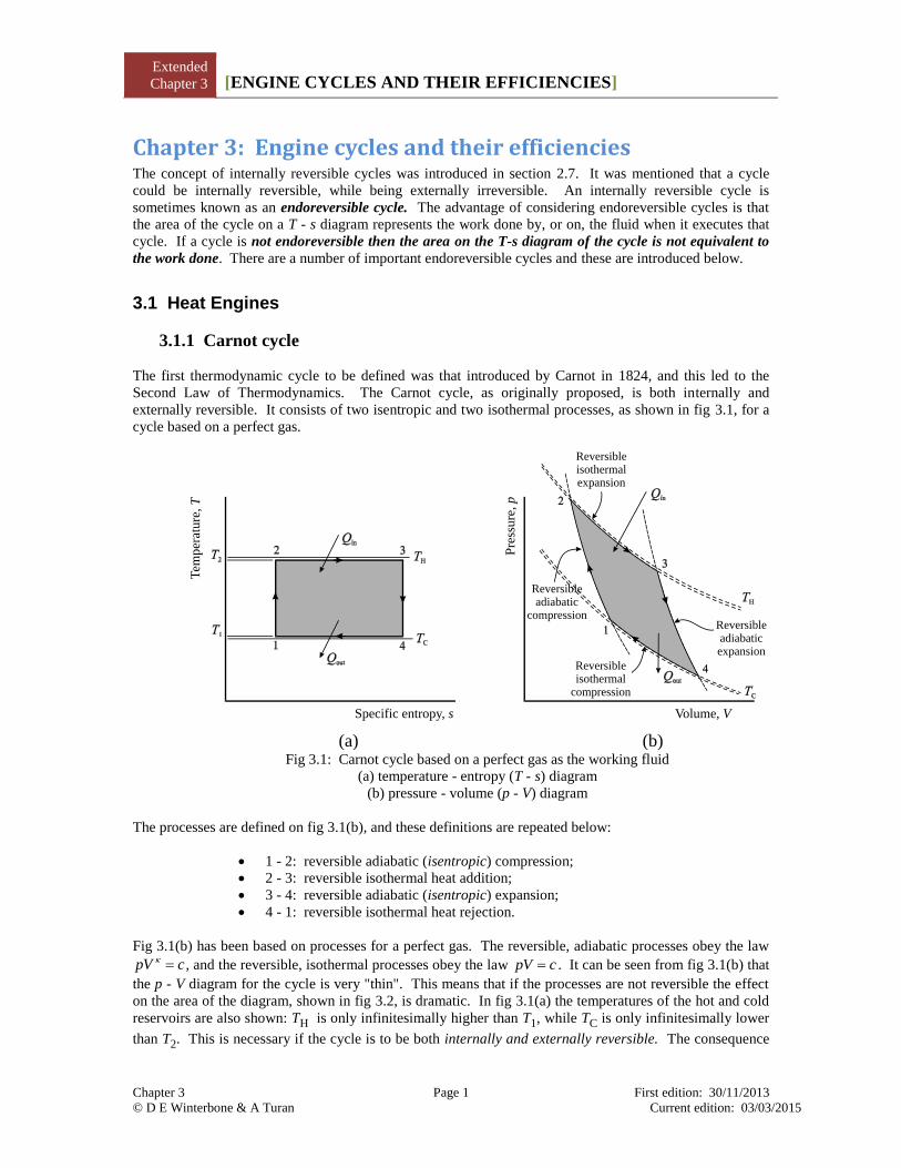
externally reversible. It consists of two isentropic and two isothermal processes, as shown in fig 3.1, for a
cycle based on a perfect gas.
Fig 3.1: Carnot cycle based on a perfect gas as the working fluid
(a) temperature - entropy (T - s) diagram
(b) pressure - volume (p - V) diagram
The processes are defined on fig 3.1(b), and these definitions are repeated below:
1 - 2: reversible adiabatic (isentropic) compression;
2 - 3: reversible isothermal heat addition;
3 - 4: reversible adiabatic (isentropic) expansion;
4 - 1: reversible isothermal heat rejection.
Fig 3.1(b) has been based on processes for a perfect gas. The reversible, adiabatic processes obey the law
pV c , and the reversible, isothermal processes obey the law pV c . It can be seen from fig 3.1(b) that
the p - V diagram for the cycle is very "thin". This means that if the processes are not reversible the effect
on the area of the diagram, shown in fig 3.2, is dramatic. In fig 3.1(a) the temperatures of the hot and cold
reservoirs are also shown: TH is only infinitesimally higher than T1, while TC is only infinitesimally lower
than T2. This is necessary if the cycle is to be both internally and externally reversible. The consequence
Tem
per
atu
re, T
Specific entropy, s
Pre
ssu
re, p
Volume, V
Reversibleisothermalexpansion
Reversibleisothermal
compression
Reversibleadiabatic
compressionReversibleadiabaticexpansion
(a) (b)

Extended
Chapter 3 [ENGINE CYCLES AND THEIR EFFICIENCIES]
Chapter 3 Page 2 First edition: 30/11/2013
© D E Winterbone & A Turan Current edition: 03/03/2015
of this is that the heat transfer rates associated with the Carnot cycle are very low, and the Carnot cycle
produces no power! The effects of external irreversibilities on engine efficiency are discussed in Chapter
6.
Fig 3.2: "Carnot cycle" depicting processes using a perfect gas working fluid, with irreversibilities
One difficulty with using a perfect gas as the working fluid is that it can only absorb heat by changing
temperature. For this reason, many of the cycles used in engines, and particularly heat engines, are based
on a fluid that can change phase during the working cycle. The working fluid most commonly used in
power generation is water, which can receive heat during the isothermal heat addition process (2 - 3) by
evaporation, and can reject it during the isothermal heat rejection (4 - 1) by condensation. The diagrams of
these cycles are shown in fig 3.3.
Fig 3.3: Carnot cycle for a working fluid which changes phase during the heat addition and
rejection processes
(a) T-s diagram for cycle; (b) p-V diagram for cycle
TH
TC 1
2 3
4
T
T1
2
Qin
Qout
Tem
per
atu
re, T
Specific Entropy, s Volume, V
Pre
ssu
re,
p
Qout
Qin
Satu
rated liq
uid
line
Saturated vapour line
2 3
41
T1
T2
TH
TC
TH
TH
TC
TC

Extended
Chapter 3 [ENGINE CYCLES AND THEIR EFFICIENCIES]
Chapter 3 Page 3 First edition: 30/11/2013
© D E Winterbone & A Turan Current edition: 03/03/2015
It can be seen that in the Carnot cycle shown on the T - s diagram the isothermal heating process now takes
place between the saturated liquid and saturated vapour lines: in other words the liquid is evaporated at the
high pressure state. This is depicted in the p - V diagram shown in fig 3.3(b).
The fluid is then expanded from state 3, on the saturated vapour line, to state 4, which is in the two-phase
liquid + vapour region. The heat rejection takes place between 4 and 1, and the fluid "condenses"
isothermally at constant pressure. The cycle is completed by a process from 1 to 2, when the fluid is
compressed reversibly and adiabatically to the saturated liquid line.
The energy transfers during the cycle can be evaluated for both cases by consideration of the T - s diagram.
The heat addition is Q T s s23 2 3 2 ; (3.1)
the heat rejection is Q T s s41 1 4 1 ( ) ; (3.2)
and the work output is W Q Q T T s s 23 41 2 1 3 2 (3.3)
The thermal efficiency of the cycle is
2 1 3 2 H C2 1
23 2 3 2 2 H
T T s s T TT TW
Q T s s T T
(3.4)
This is the same as the thermal efficiency of a reversible cycle derived by reference to the definition of the
absolute scale of temperature in section 2.5, eqn 2.6. These energy transfers can be illustrated on a T - s
diagram, as shown on fig 3.4.
Fig 3.4: Energy transfer processes depicted on T - s diagram
23
41
Heat addition, area 6 2 3 5 6
Heat rejection, area 6 1 4 5 6
Work output, area 1 2 3 4 1
Q
Q
W
The thermal efficiency of the reversible cycle based on a perfect gas can also be evaluated. It should be
realised that the thermodynamic scale of temperature and "absolute temperature" defined by the perfect gas
T
T
Q
Q
Tem
per
ature
, T
Specific entropy, s
Sat
ura
ted
liqu
id li
ne Saturated vapour line
W
Extended
Chapter 3 [ENGINE CYCLES AND THEIR EFFICIENCIES]
Chapter 3 Page 4 First edition: 30/11/2013
© D E Winterbone & A Turan Current edition: 03/03/2015
law are the same by coincidence rather than definition. Considering the processes shown in fig 3.1(b), the
work transfers are defined by the areas of the p - V diagram.
Work done,
Wp V p V
W p VV
VW
p V p VW p V
V
V12
1 1 2 223 2 2
3
2
343 3 4 4
41 4 41
41 1
; ln ; ; ln
;
which gives the work from the cycle as
12 23 34 41
cycle.W W W W W
Now
Wp V p V R T T
WR T T
121 1 2 2 1 2
34
3 4
1 1 1
, and ,
which means that W W W W12 34 12 34 0 , . giving
Also 3 3 123 2 2 2 41 1
2 2 4
ln ln , and lnV V V
W p V RT W RTV V V
,
giving 3
2 1cycle
2
lnV
W R T TV
. (3.5)
The energy addition to the cycle can be evaluated from process 2 - 3. Applying the First Law
gives
Q dU W c T T W W
RTV
V
v23 23 23 3 2 23 23
23
2
ln (3.6)
Hence, the thermal efficiency of the cycle is cycle C2 1 1
23 2 2 H
1 1
WTT T T
Q T T T
. (3.7)
This is the same as evaluated from the previous analysis, and given as eqn 3.4, which is not surprising
because all reversible cycles operating between the same temperature limits have the same thermal
efficiency. Hence, the efficiency of a reversible cycle is independent of the working fluid.
It can be seen that there are a number of benefits in using a working fluid which can change phase,
including:
constant pressure isothermal heat addition;
a diagram that is less sensitive to inefficiencies than the perfect gas one;
it is possible to replace the compression of a gaseous phase by the pumping of a
liquid, in which case the compression work is significantly reduced..
The work output of a Carnot cycle is defined by the areas of either a p - V or a T - s diagram, and it can be
seen that these are finite. However, while the Carnot cycle can produce a finite work output, the power
output is zero because the rate of heat transfer to the engine across an infinitesimal temperature
difference is zero. The temperature difference is zero to achieve external reversibility. This means that the
Carnot efficiency defines the maximum efficiency of a heat engine between two temperature levels. This is
never achieved in practice because all engines are, at least, significantly irreversible in the external heat
transfer processes: this is discussed in Chapter 6.
3.1.2 Rankine cycle
It was shown above that the Carnot cycle for a fluid which changes phase during the working cycle requires
an expansion device which operates with a fluid with a low quality (x) at the end of the expansion process.
This tends to create problems in the design of the expansion device because of the amount of liquid in the
working fluid. In the case of a steam turbine there can be very bad erosion of the low-pressure turbine
blades due to water droplets in the steam, and this can reduce the reliability of the machine. Similarly, the

Extended
Chapter 3 [ENGINE CYCLES AND THEIR EFFICIENCIES]
Chapter 3 Page 5 First edition: 30/11/2013
© D E Winterbone & A Turan Current edition: 03/03/2015
compression depicted in fig 3.3 goes from a low quality mixture of water and water vapour (at state 1) to
saturated liquid water (at state 2). This requires careful control of state 1 to ensure that state 2 lies on the
saturated liquid line, and also a compressor that can deal with a mixture that changes phase during the
compression process. Both of these problems can be solved, at least partially, by use of the Rankine cycle.
The Rankine cycle is the basis of all steam turbine power plants, and a schematic diagram of a steam
turbine power plant is shown in fig 3.5. It is an adaptation of the Carnot cycle to remove some of the
latter's limitations. The basic Rankine cycle (see fig 3.6(a)) removes the problem of compressing a two-
phase liquid from 1 to 2. In this case the fluid is condensed right up to the saturated liquid line (state 1). It
is then compressed in the liquid phase from 1 to 2, where it is a compressed liquid. Heating, at constant
pressure, commences at 2, and the fluid is raised in temperature from 2 to 3, with evaporation occurring
from 3 to 4. At state 4 the liquid is fully evaporated, and state 4 is on the saturated vapour line. The fluid
is expanded from 4 to 6 in the turbine, when it experiences the same change of state as in the Carnot cycle.
the fluid at 6 is very wet and turbine blade erosion can be a problem. This situation can be improved by
superheating the fluid from state 4 to state 5, as shown in fig 3.6(b). The effect of this is to raise the
maximum temperature achieved by the fluid in executing the cycle, and the peak temperature is now T5
rather than T2, as it was in the other cycles up till now.
Fig 3.5 Schematic diagram of a steam turbine power plant
The work output of an endoreversible Rankine cycle is defined by the area of the T-s diagram. This means
that for the same pressures it is possible to increase the power output of the cycle by superheating, because
the area of the diagram in fig 3.6(b) is greater than that in fig 3.6(a). Hence, superheating increases the
work output, but what is the effect on the efficiency? First, it must be recognised that the energy input is
greater in the superheat cycle than the standard one, and is defined by the enthalpy difference between 2
and 5, rather than 2 and 4. The real question is has the energy added between 4 and 5 in fig 3.6b been used
more efficiently than that between 2 and 4. This can be answered by considering the superheat cycle to be
made up of two cycles: 1-2-3-4-5-6-1, and 6'-4-5-6-6'. The first cycle here is the basic Rankine cycle,
while the second is a superheated cycle. Since the efficiency of a heat engine cycle is dependent on the
temperature at which energy is received the efficiency of cycle 6'-4-5-6-6' is greater than that of cycle 1-2-
3-4-5-6-1 and, hence, the efficiency of the superheated cycle is greater than that of the basic one.
W netSteam plant
Q in
Q out
(a)
(b)
W netQout
Turbine
Feedpump
Condenser
Boiler
system aSystem b
W Turbine
W Feedpump
Qi n
1
2
3
4

Extended
Chapter 3 [ENGINE CYCLES AND THEIR EFFICIENCIES]
Chapter 3 Page 6 First edition: 30/11/2013
© D E Winterbone & A Turan Current edition: 03/03/2015
Fig 3.6: The Rankine cycle
(a) the basic Rankine cycle
(b) the Rankine cycle with superheat
3.1.3 Comparison of efficiencies of Carnot and Rankine cycles
It is possible to use a simple analysis to compare the efficiencies of Carnot and Rankine cycles operating
between the same temperature limits. Two cycles are shown superimposed in figs 3.7(a) and (b), which
show the basic and superheated cycles respectively.
Fig 3.7: Comparison of Carnot and Rankine cycles
(a) basic Rankine cycle; (b) Rankine cycle with superheat
The Carnot cycle operating between the same temperature limits produces more work than the Rankine
cycle, but this does not guarantee that the efficiency is higher. The efficiency can be considered by
examining the work output and the heat rejected. By definition, the efficiency of a heat engine is
in out
.W W
Q W Q
In these cases the values of Qout for the Carnot and Rankine cycles are the same,
and, hence, the efficiency of the Carnot cycle must be greater than that of the Rankine cycle.
Carnot Rankine (3.8)
T3
T1
Tem
per
atu
re,
T
Specific entropy, s
Q
Qo u t
WP
Saturatedliquid line
Saturatedvapour line
WT
T3
T1
Qi n
Qo u t
Tem
per
atu
re, T
Specific entropy, s
W
Saturatedliquid line
Saturatedvapour line
WT
T5
T3
T1
Qi n
Qo u t
Tem
per
atu
re,
T
Specific entropy, s
WP
Saturatedliquid line
Saturatedvapour line
WT
T3
T1
Qi n
Qo u t
Tem
per
atu
re, T
Specific entropy, s
WP
Saturatedliquid line
Saturatedvapour line
WT
T5
Additionalwork
Additionalwork
Extended
Chapter 3 [ENGINE CYCLES AND THEIR EFFICIENCIES]
Chapter 3 Page 7 First edition: 30/11/2013
© D E Winterbone & A Turan Current edition: 03/03/2015
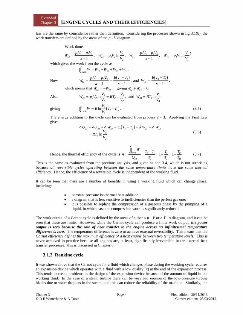
Another way of looking at this problem is to consider the mean temperature of energy addition.
3.1.4 Mean temperature of energy addition and rejection
It was shown in figs 3.7(a) and (b) that the Carnot cycle has a greater thermal efficiency than a Rankine
cycle operating between the same temperature limits. This is because the heat addition for the Carnot cycle
takes place at the maximum temperature of the cycle, and the heat rejection occurs at the minimum
temperature. Hence, the Carnot cycle takes maximum advantage of the temperature difference. The
Carnot cycle in fig 3.8(a) has been broken down into an infinite number of infinitesimal cycles, and the
efficiency of the cycle is given by
cycles
cycles
W
Q
. (3.9)
Since all the cycles are identical in this case the efficiency of the whole cycle is equal to the individual
efficiencies of the incremental cycles.
The situation changes with the superheated Rankine cycle in fig 3.8(b). Three incremental cycles have
been depicted. Cycle a is in the region where the liquid water is being heated, and the efficiency is low
because the peak temperature is low. The next cycle, b, is in the evaporation region, and the efficiency in
this region will be the same as the Carnot cycle shown in fig 3.8(a). The final cycle, c, has been drawn in
the superheat region, where the temperature is again rising. The efficiency of this cycle will be higher than
during the evaporation region but lower than that of a Carnot cycle operating between T1 and T5. Hence,
the efficiency of the Rankine cycle in fig 3.8(b) will be an "average" of the incremental cycles which make
up the whole Rankine cycle. Since the temperature of heat rejection in this diagram is the same for all
incremental cycles then the efficiency is governed by the temperature of energy addition. The efficiency of
each incremental cycle is equivalent to that of the equivalent Carnot cycle, and the work output of each
cycle is
(3.10)
a
r
where temperature of heat addition
temperature of heat rejection
T
T
Fig 3.8: Carnot and Rankine cycles broken down to incremental Carnot cycles
Now, the heat addition for each incremental cycle is δ δQ T s , and, hence, the work done over the cycle
is
T2
T1
Qi n
Qo u t
Tem
per
atu
re, T
Specific entropy, s
Saturatedliquid line
Saturatedvapour line
T3
T1
Qi n
Qo u t
Tem
per
atu
re, T
Specific entropy, s
Saturatedliquid line
Saturatedvapour line
T5
Incrementalcycles
Incrementalcycles
r aδ δ 1 ,W Q T T

Extended
Chapter 3 [ENGINE CYCLES AND THEIR EFFICIENCIES]
Chapter 3 Page 8 First edition: 30/11/2013
© D E Winterbone & A Turan Current edition: 03/03/2015
cycle a r acycle cycle
5
a r a r 5 2cycle 2
5
a2
r 5 25 2
δ 1 d
d d
d
W W T T T s
T T s T s T s s
T sT s s
s s
(3.11)
This equation is equivalent to eqn (3.3), but the value of the high temperature has been replaced by the term
5
a2
5 2
dT s
s s
, which is the mean temperature of heat addition.
Mean temperature of energy addition, or rejection;
2
1
2 1
dT sT
s s
(3.12)
Hence, any cycle can be made equivalent to a Carnot cycle, and the efficiency of that cycle is the same as
that of a Carnot cycle with the same mean temperatures of heat addition and rejection. This shows that
any cycle in which the temperature of heat addition and rejection are not constant cannot achieve the same
efficiency as a Carnot cycle with the same temperature limits.
3.1.5 Rankine cycle depicted on p-V-T surface
The diagrams given above show the Rankine cycle on T-s diagrams. This is the normal manner in which
the cycle is shown. It is also possible to draw the Rankine cycle on the p - v - T surface for water, as shown
in fig 3.9.
Fig 3.9: Rankine cycle shown on p - V - T surface
Critical point
Pre
ssu
re
Volume

Extended
Chapter 3 [ENGINE CYCLES AND THEIR EFFICIENCIES]
Chapter 3 Page 9 First edition: 30/11/2013
© D E Winterbone & A Turan Current edition: 03/03/2015
3.2 Air standard cycles
The Rankine cycle is based on a working fluid which changes phase during the cycle. This has the
advantage of introducing regions of heat addition and rejection where the temperature is constant.
However, the most readily available working fluid is air, which is a superheated gas at normal operating
conditions. This results in a series of cycles in which the energy is received and rejected at variable
temperature. These cycles can be used to examine the performance of internal combustion engines, e.g.,
petrol and diesel engines, and gas turbines. It should be realised that internal combustion engines and gas
turbines are not heat engines - because mass flows across the boundaries as air and fuel to enter the
engines, and exhaust gases leave. More realistic cycles for these engines are considered in Chapters 16 and
17, respectively. However, it is possible to define "engines" which can be analysed by endoreversible
cycles: these "engines" replace the energy flows brought about by gas flows and combustion by heat
transfer processes. Such cycles will be described below.
There are three air-standard cycles:
constant volume ‘combustion’(Otto)
constant pressure ‘combustion’ (Diesel)
dual ‘combustion’ – this is a combination of constant volume and constant
pressure combustion, and results in a slightly more realistic cycle
These are the heat engine equivalent of the reciprocating engine and different from the actual engine cycle
because:-
the cycle is a closed one with heat transfer;
the working fluid does not change composition;
the energy addition obeys closely defined rules e.g. constant volume energy
addition;
the rates of heat release (energy addition) are unrealistic;
indicated work outputs are evaluated.
In a real cycle:
• the fluid changes as the gas passes through the engine;
• the properties of the fluid change;
• the rates of heat release are finite;
• the engine has frictional and heat transfer losses.
The effect of two of these differences will be examined in Chapter 14:
(i) frictional losses;
(ii) the finite rate of heat release.
3.2.1 Otto cycle
The Otto cycle is an air standard cycle which approximates the processes in petrol or diesel engines. It is
based on constant volume heat addition (combustion) and heat rejection processes, and isentropic
compression and expansion. The diagram is shown on fig 3.10, where it is superimposed on an actual p - V
diagram for a diesel engine.
The actual p-V diagram for an engine has rounded corners because of the processes of combustion take
place at a finite rate. The Otto cycle has sharp corners because the "combustion" is switched on and off
instantaneously. It can be seen from fig 3.10 that the area of the Otto cycle is larger than that of the actual
cycle, and this has to be taken into account when analysing engine cycles – the actual cycle will always
produce less work output than the Otto cycle.

Extended
Chapter 3 [ENGINE CYCLES AND THEIR EFFICIENCIES]
Chapter 3 Page 10 First edition: 30/11/2013
© D E Winterbone & A Turan Current edition: 03/03/2015
Fig 3.10: Otto cycle and engine cycle on p - V diagram
A typical engine "cycle" is defined in fig 3.11. It consists of a compression stroke (fig 3.11a), followed by
a period of combustion close to top dead centre (tdc) (fig 3.11b), and then by expansion (fig 3.11c). These
two strokes form the power producing processes, but afterwards the products of combustion have to be
replaced by fresh air. This is symbolised in fig 3.11d, where the exhaust valve is open at the beginning of
the exhaust stroke. In a four-stroke engine the piston executes two complete revolutions of the crankshaft,
and uses two-strokes while the gas is pushed out by the piston on the up stroke, and then the intake valve is
opened to enable air to be induced. In a two-stroke engine the intake and exhaust strokes occur at the end
and the beginning of the expansion and compression strokes, respectively. These processes are called the
gas exchange processes, and are one of the main reasons why real engines are not heat engines. The other
reason is the combustion process, when the air is used to burn the fuel. This process of combustion means
that the fluid in the engine cannot undergo a cycle.
Fig 3.11: Processes in a reciprocating engine (i.e. a diesel or petrol engine)
0 0.0005 0.0010 0.0015 0.0020 0.0025 0.0030
0
20
40
60
80
100
120
140
160
180
Pre
ssure
, /
(bar
)p
Volume, / (m )V3
constantvolume
combustion
Isentropiccompression
andexpansion
(a) (b) (c) (d)
Compression Combustion ExpansionExhaust
and induction

Extended
Chapter 3 [ENGINE CYCLES AND THEIR EFFICIENCIES]
Chapter 3 Page 11 First edition: 30/11/2013
© D E Winterbone & A Turan Current edition: 03/03/2015
The Otto, Diesel and dual-combustion cycles are air standard cycles that approximate the processes in a
real engine. They can be achieved in the following way:
the combustion process is replaced by a heat transfer process in which an amount of
energy equivalent to the energy released by combustion is added to the air;
the gas exchange process is replaced by a heat transfer process to a cold reservoir, so that
the hot gases after expansion are returned to the state of the air after induction
The resulting air standard cycle is defined in fig 3.12.
Fig 3. 12: Method of achieving air standard cycle for Otto cycle
The basic Otto cycle is made up of four processes:
isentropic compression;
constant volume heat addition;
isentropic expansion;
constant volume heat rejection.
These can be depicted on T - s and p - V diagrams as shown in fig 3.13.
Since all the processes in fig 3.13 are reversible, the areas of the diagrams (a and b) are equal, and depict
the work done in the cycle. The work done is
2 4
1 3
3 3 4 41 1 2 21 2 3 4
d d d
1 1 1
W p V p V p V
p V p Vp V p V mRT T T T
(3.13)
The energy added to the cycle is that added at constant volume between 2 and 3, and is given by
Q mc T TmR
T Tv23 3 2 3 21
( )
(3.14)
Hence the thermal efficiency is
(a) (b) (c) (d)
Compression
Hotreservoir
Expansion
Coldreservoir

Extended
Chapter 3 [ENGINE CYCLES AND THEIR EFFICIENCIES]
Chapter 3 Page 12 First edition: 30/11/2013
© D E Winterbone & A Turan Current edition: 03/03/2015
1 2 3 4 4 1
Otto
23 3 2 3 2
d1
heat rejected1
heat added
p V T T T T T T
Q T T T T
(3.15)
This equation can be rearranged into the more familiar one for the Otto cycle in the following way. First, it
is necessary to define the compression ratio, r, which is based on the ratio of the volume at ‘top dead
centre’ (tdc) to that at bottom dead centre (bdc), i.e. r V V 2 1 . It is then possible to write the temperatures
around the cycle in terms of T T r1 3 and , and the compression ratio, . This gives
TT
rT T r4
3
1 2 1
1
, and , which may be substituted into eqn (3.15) to give
311
4 1
Otto 13 2 3 1
1
3 1
1 1 1
3 1
1 1
1 11 1
TTT T r
T T T T r
T T r
r T T r r
(3.16)
Fig 3.13: Otto cycle
(a) T-s diagram; (b) p-V diagram
Now, the term
11
1
2
4
3r
T
T
T
T , and hence 1 4
Otto2 3
1 1 .T T
T T (3.17)
Thus, the efficiency of an Otto cycle is also related to a temperature ratio, but in this case it is the
temperature ratio due to isentropic compression or expansion. Consideration of fig 3.13(b) shows that this
is significantly less than the temperature ratio of the hot and cold reservoirs, and hence the efficiency of the
Otto cycle is less than that of a Carnot cycle operating between the same two temperature limits which has
an efficiency, C 1
Carnot
H 3
1 1T T
T T . The reason for this is simply that the heat is added and rejected
over varying temperatures, and it can be shown that the efficiency of an engine operating on an Otto cycle
Pre
ssu
re, p
Volume, V
Tem
per
atu
re,
T
Specific entropy, s
Constantvolume
Isentropic
Isentropic
Constantvolume
(a) (b)
Ta
_
T_
r
Incrementalcycle

Extended
Chapter 3 [ENGINE CYCLES AND THEIR EFFICIENCIES]
Chapter 3 Page 13 First edition: 30/11/2013
© D E Winterbone & A Turan Current edition: 03/03/2015
is the same as a Carnot cycle operating between reservoirs at the mean temperatures of heat addition
(�̅�𝑎)and rejection(�̅�𝑟). It is interesting to note that the efficiency of the Otto cycle approaches that of the
Carnot cycle if T T3 2 ; such a cycle produces no output because lines 1-2 and 3-4 on fig 3.13 become
coincident.
3.2.2 Diesel cycle
The diesel cycle is also a cycle applied to reciprocating engines, and is similar to the Otto cycle except that
the heat is applied at constant pressure rather than constant volume. This removes the limitation of infinite
rates of combustion implied by the Otto cycle, but still results in an unrealistic combustion pattern. The
diesel cycle is shown in fig 3.14.
Fig 3.14: Diesel cycle
(a) T-s diagram; (b) p-V diagram
The work done in a diesel cycle is
3 3 4 41 1 2 2
2 3 2
3 31 1 4 4
2 2
2 2 2 2 2 2
2
1
2
1
d1 1
11 1
1
11 1 1
1
11 1
1
p V p Vp V p VW p V p V V
p Vp V p Vp V
p V p V p V
mRTr r
rr
mRT
r
(3.18)
where defines the size of the constant pressure heat addition region, V V3 2 . The effect of the constant
pressure heat addition region is to reduce the expansion ratio of the cycle, e 4 3r V V r . This has a
large effect on the efficiency of the cycle.
The heat addition is
Q mc T Tm R
T Tm RT
p23 3 2 3 22
1 11
( )
. (3.19)
The efficiency of the cycle is
Pre
ssure
, p
Volume, V
Tem
per
atu
re,
T
Specific entropy, s
Constantvolume
Isentropic
Isentropic
Constantvolume
(a) (b)
Constantpressure
Constantpressure
Incremental cycle

Extended
Chapter 3 [ENGINE CYCLES AND THEIR EFFICIENCIES]
Chapter 3 Page 14 First edition: 30/11/2013
© D E Winterbone & A Turan Current edition: 03/03/2015
1
diesel 1
23
11d 1 1
1 .1 1
p Vr
Q r
(3.20)
This efficiency is less than that of the Otto cycle because the term
11
1
3.2.3 Dual combustion cycle
The dual-combustion cycle is shown in Fig 3.15. The cycle gets its name because a proportion of the
‘combustion’ (heat addition) takes place at constant volume, from 2 to 3, and then the remainder occurs at
constant pressure, from 3 to 4. This cycle is the most representative of real engine cycles, in which the
initial combustion takes place rapidly, and then slows down later in the process (although the dual-
combustion cycle requires the heat release to increase as the volume increases). It can be shown (this is
left to the reader) that the efficiency of a dual-combustion cycle is
th 1
1 11
1 1r
(3.21)
where = 𝑝3 𝑝2⁄ , the pressure ratio caused by constant volume combustion.
Fig 3.15 The dual-combustion cycle
3.2.4 The most efficient internal combustion engine cycle - based on various
constraints
In the case of ideal cycles it is possible to define the relationship between the thermal efficiency (indicated)
and the compression ratio. The indicated thermal efficiency for an Otto cycle (constant volume
combustion), shown in Fig.3.13, is given by eqn (3.16)
th 1
11
r
Pre
ssu
re,
p
Volume, V
Tem
per
ature
, T
Specific entropy, s
Constantvolume
Isentropic
Isentropic
Constantvolume
(a) (b)
Constantpressure
Constantpressure
Incremental cycle
VV2 e

Extended
Chapter 3 [ENGINE CYCLES AND THEIR EFFICIENCIES]
Chapter 3 Page 15 First edition: 30/11/2013
© D E Winterbone & A Turan Current edition: 03/03/2015
where r = compression ratio;
= ratio of specific heats (cp/cv).
The indicated thermal efficiencies of the diesel and dual combustion cycles are lower than that of the Otto
cycle for the same compression ratio. The relationships for these cycles are:
Constant pressure cycle (diesel cycle), shown in Fig. 3.14 – efficiency given by eqn (3.20):
th 1
1 11
1r
(3.20)
where = cut-off ratio.
Dual combustion cycle, shown in fig. 3.15 – efficiency given by eqn (3.21),
th 1
1 11
1 1r
(3.21)
where = pressure ratio caused by constant volume combustion.
Equations 3.16, 3.20, 3.21 define the efficiency of air-standard cycles. These can be generalized as:
th 1
C1
r
(3.22)
where C = 1 for Otto cycle (3.23)
1C 1
1 1
for a dual combustion cycle; (3.24)
1C 1
1
, for a diesel (constant pressure) cycle. (3.25)
Hence, for a given compression ratio (r) the thermal efficiencies are related by
th th thOtto dual comb diesel (3.26)
However, the situation changes if the maximum pressure is limited: in fact, if all three cycles are compared
for the same peak pressure and same work output then
th th thdiesel dual comb Otto (3.27)
Why is this the case? Considering first the cycles with the same compression ratio, then it is apparent that
the average expansion ratio of each of the cycles is different. The average expansion ratio of the Otto cycle
is equal to the compression ratio, r. In fig. 3.15, Ve represents a typical cycle and the typical expansion
ratio r V Ve e
1 and, since Ve > V2, then re < r. So if there is any constant pressure combustion then there
must be a lower mean expansion ratio than in the case of the Otto cycle.

Extended
Chapter 3 [ENGINE CYCLES AND THEIR EFFICIENCIES]
Chapter 3 Page 16 First edition: 30/11/2013
© D E Winterbone & A Turan Current edition: 03/03/2015
Fig 3.16 Comparison of Otto and Diesel cycles with the same maximum pressure and work outputs
Fig. 3.16 shows a comparison of two cycles (an Otto and a Diesel cycle). These have the same peak
pressure and the same work output. It can be seen that the compression ratio of the diesel engine is higher
than that of the Otto cycle engine: in fact, the expansion ratio of the diesel cycle throughout the cycle is
higher than the compression ratio of the Otto cycle. This means that the thermal efficiency of each element
of the diesel cycle is more efficient than the Otto cycle, and hence this diesel cycle is more efficient than
the Otto cycle. A similar argument applies for the dual combustion cycle, which lies between the diesel
and Otto cycles.
It is useful to consider these idealised cycles because they enable general concepts to be understood. They
have enabled us to see why a diesel engine cycle can be more efficient than an Otto one if the peak pressure
is limited. They have shown that expansion ratio is a more relevant parameter than compression ratio when
considering the efficiency of a cycle. However, they have not allowed us to see how the performance of
real engines, with finite rates of combustion, varies when parameters are changed. These are considered in
Chapter 16, by means of an engine simulation progam. The results of the simulation are presented in a
form that should be intelligible to the reader of this chapter, without having assimulated all necessary
theory to understand the detailed workings of the program.
In the previous sections engines have been compared based on their efficiencies. Another way of assessing
the output of reciprocating engines is to compare them on the basis of mean effective pressure (mep). The
indicated mean effective pressure of an engine (imep, ip ) is defined as the average (mean) pressure that
would have to operate over the whole stroke (S 1 2V V V ) to give the same work output as the actual cycle,
i.e.
i
S
dp Vp
V
(3.28)
The concept of mean effective pressures will be returned to in Chapter 16.
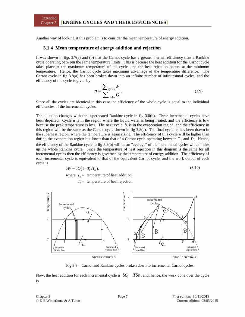
3.2.5 Joule (or Brayton) cycle
The Joule cycle is the air standard cycle which describes the processes in the gas turbine. The Joule cycle
has constant pressure combustion and constant pressure heat rejection. It is depicted in fig 3.17.
This cycle, which is examined in exactly the same manner as the Otto and diesel cycles in Chapter 16.2,
results in the following expression for efficiency eqn (17.8))
Pre
ssu
re,
p
Volume, V
Maximum pressure
Extended
Chapter 3 [ENGINE CYCLES AND THEIR EFFICIENCIES]
Chapter 3 Page 17 First edition: 30/11/2013
© D E Winterbone & A Turan Current edition: 03/03/2015
Joule 1
p
11
r
, (3.29)
where p 2 1, the pressure ratio for the gas turbiner p p .
The term 1
p
1
r
is equivalent to the temperature ratio,
𝑇1
𝑇2 , and the significance of this is discussed below.
Fig 3.17: Joule (gas turbine) cycle
(a) T-s diagram; (b) p-V diagram
3.3 General comments on efficiencies
The efficiency of the Carnot cycle is directly related to the temperature ratio of the hot and cold reservoirs.
Examination of the other efficiencies will show that they are also related to temperature ratios of the cycle.
The efficiency of the Otto cycle is (eqn (3.17))
1 4Otto 1
2 3
11 1 1
T T
T Tr
.
The equation for the diesel engine is more complex and will not be considered here. However, the
efficiency of the Joule cycle can also be related to the temperature ratio because
1
2p
1
Tr
T
, and hence
1 4Joule 1
2 3
p
11 1 1 ,
T T
T Tr
on fig 3.17.
Hence, all heat engines have efficiencies of the form
nth
m
1 , T
T
Pre
ssure
, p
Volume, V
Tem
per
atu
re,
T
Specific entropy, s
Isentropic
Isentropic
(a) (b)
Constantpressure
Constantpressure

Extended
Chapter 3 [ENGINE CYCLES AND THEIR EFFICIENCIES]
Chapter 3 Page 18 First edition: 30/11/2013
© D E Winterbone & A Turan Current edition: 03/03/2015
where Tn and Tm are particular temperatures relating to the individual cycle.
3.4 Reversed heat engines
Reversed heat engines were introduced in section 2.7, and comprise refrigerators and heat pumps. The
objectives of these devices are to transfer energy from a low temperature reservoir to a higher temperature
one. In the case of the refrigerator the aim is to cool the ice box, and reject the energy extracted from it into
ambient conditions at a higher temperature. The purpose of the heat pump is to warm a building by
"pumping" low grade energy up to a higher temperature. Both of these devices work by using power input
to drive the processes: it is not possible, by the Second Law, for energy to pass from a low to a higher
temperature reservoir. The cycles used to analyse reversed heat engines are similar to those introduced
above for heat engines producing power - the processes are simply executed in reverse order.
3.4.1 Reversed Carnot cycle
If the Carnot cycle shown in fig 3.1 is operated in reverse, i.e. the arrows on the diagram are turned round,
as in fig 3.16, then the directions of the work and heat transfer terms are also reversed. This means that net
work is provided to the cycle during processes 1-2 and 3-4, and that energy Qin is "pumped" from the low
temperature reservoir (TC), and energy Qout is delivered to the high temperature reservoir TH. Hence, the
addition of work to the cycle is able to raise the "quality" of the energy in the low temperature reservoir.
Fig 3.18: T - s diagram for reversed heat engine (refrigerator or heat pump) operating on reversed
Carnot cycle
3.4.2 Actual refrigerator and heat pump cycles
A device which would execute this cycle is shown schematically in fig 3.19(a): in this case, unlike that of
the steam turbine, the pumping work is significantly larger than the work obtained from the expander
turbine. In most small, domestic, refrigeration plant the expander turbine is replaced with throttle, as
shown in fig 3.19(b). This modifies the T - s diagram for the refrigerator to that given in fig 3.20(a). Many
refrigeration plants operate with sub-cooling of the working fluid, which further modifies the cycle to that
in fig 3.20(b).
As described in Section 2.7.1, thermal efficiency is not the correct parameter to use to define the
"efficiency" of a reversed cycle, and the parameter used in this case is the coefficient of performance,
which is defined as

Extended
Chapter 3 [ENGINE CYCLES AND THEIR EFFICIENCIES]
Chapter 3 Page 19 First edition: 30/11/2013
© D E Winterbone & A Turan Current edition: 03/03/2015
C C
net H C
Heat transferred from cold reservoir
Net work done
, for a refrigeratorQ Q
W Q Q
H H
net H C
Heat transferred to hot reservoir'
Net work done
, for heat pumpQ Q
W Q Q
.
It was also shown in Section 2.7.1 that ' 1. The coefficients of performance of all reversible heat
engines operating between the same two temperature reservoirs will be equal, irrespective of the working
fluid. This can be defined in terms of the reservoir temperatures if the devices are internally and externally
reversible. Substituting for temperatures gives
C
H C
T
T T
, and H
H C
'T
T T
.
Fig 3.19 Schematic diagrams of refrigerator (or heat pump)
(a) with expander turbine (b) with throttle
3.4.3 Example:
Calculate the coefficients of performance of the refrigerator and heat pump working with
ammonia as the refrigerant. The evaporation takes place at a pressure of 0.7177 bar, after which
the ammonia is compressed isentropically to the saturated vapour line at a pressure of 15.54 bar.
After constant pressure condensation to a temperature of 28C, the fluid is expanded irreversibly
through a throttle to the evaporator pressure.
Solution:
The T - s diagram for the cycle is shown in fig 3.20.
The values of properties at the salient points can be obtained from tables of properties.
Conditions at 4:
Pump
Condenser
W Pump
Qi n
Q out
System boundary
Throttlevalve
Ice box
Evaporator
Pump
Condenser
W Pump
Qi n
Q out
System boundary
Ice box
Evaporator
WExpander
Expanderturbine
(a) (b)

Extended
Chapter 3 [ENGINE CYCLES AND THEIR EFFICIENCIES]
Chapter 3 Page 20 First edition: 30/11/2013
© D E Winterbone & A Turan Current edition: 03/03/2015
4 1
f g fg
f fg g
0.7177bar;
0kJ/kg; 1390kJ/kg; 1390kJ/kg
0kJ/kgK; 5.962kJ/kgK; 5.962kJ/kgK
p p
h h h
s s s
The values of enthalpy and entropy on the saturated liquid line at 40C have been arbitrarily set at
zero in the tables.
Conditions at 3:
3 2
f g
f g
15.54bar
371.9kJ/kg; 1473.3kJ/kg
1.360kJ/kgK; 4.877kJ/kgK
p p
h h
s s
Fig 3.20: Irreversible refrigeration cycles
(a) with simple throttle (see fig 3.19b)
(b) with throttle and sub-cooling
Fig 3.21: T - s diagram for reversed heat pump cycles.
Conditions at 2:
T3
T1
Qi n
Qo u t
Tem
per
ature
, T
Specific entropy, s
Saturatedliquid line
Saturatedvapour line
WC
Throttling
Condensation
Evaporation
(a)
T3
T1
Qo u t
Tem
per
ature
, T
Specific entropy, s
Saturatedliquid line
Saturatedvapour line
WC
Throttling
Condensation
Evaporation
(b)
TH
TC
Qi n
Qo u t
Tem
per
ature
, T
Specific entropy, s
Saturatedliquid line
Saturatedvapour line
WCThrottling
Condensation
Evaporation
Sub-cooling
- 48 C0
40 C0
28 C0 p
3 = 15.54 bar
p1 = 0.7177 bar
Extended
Chapter 3 [ENGINE CYCLES AND THEIR EFFICIENCIES]
Chapter 3 Page 21 First edition: 30/11/2013
© D E Winterbone & A Turan Current edition: 03/03/2015
This is a sub-cooled state where the liquid is compressed, and it will be assumed that the enthalpy
is equal to the enthalpy on the saturated liquid line at 28C. Hence
f 313.4kJ/kgh
Now, since the compression from 4 to 3 is isentropic s s4 3 . Hence,
3 g f4.877 1 5.962
giving 4.877 5.962 0.8180
s xs x s x
x
and 4 g f1 0.8180 1390 1137kJ/kgh xh x h
Work done in compressor
C 43 4 3 1137 1473.3 336.3kJ/kgW W h h
Heat extracted from the evaporator (cold reservoir)
C 41 4 1 4 2 1137 313.4 823.6kJ/kg.Q Q h h h h
Hence, coefficient of performance of refrigerator
h h
h h
4 1
3 4
823 6
336 32 449
.
..
Heat transferred from the condenser (hot reservoir)
H 32 2 3 313.4 1473.3 1159.9kJ/kgQ Q h h
Hence, coefficient of performance of heat pump, '.
..
h h
h h
2 3
4 3
1159 9
336 33 449
Thus, both the coefficients of performance are greater than unity, and the coefficient of
performance of the heat pump is one greater than that of the refrigerator - even though the devices
are not reversible. If the devices had been reversible, i.e. had followed the reversed Carnot cycle,
then the values would have been
C 1
H C 3 1
3H
H C 3 1
2332.913
313 233
313' 3.913
313 233
T T
T T T T
TT
T T T T
It can be seen that the reversible reversed heat engines, operating on the Carnot cycle, have higher
coeffficients of performance than those undergoing cycles with irreversibilities.
3.5 Concluding remarks This chapter has introduced a range of different cycles, from the fundamental Carnot cycle through more
realistic cycles for simulating actual powerplant. It is possible to evaluate the thermal efficiency of these
cycles, and these efficiencies can be compared to that of the Carnot cycle. The Carnot cycle is shown to be
the most efficient cycle operating between two temperature levels, simply because it is able to receive and
reject energy at the upper and lower temperatures. None of the other cycles can achieve this, although the
basic Rankine cycle can come close.

Extended
Chapter 3 [ENGINE CYCLES AND THEIR EFFICIENCIES]
Chapter 3 Page 22 First edition: 30/11/2013
© D E Winterbone & A Turan Current edition: 03/03/2015
Air standard cycles have been introduced, and cycles that can be used to analyse reciprocating engines, e.g.
spark ignition and diesel engines, and gas turbines have been described. It has been explained that engines
following these cycles are usually not heat engines because working fluid flows across their boundaries. It
has also been demonstrated that they can never achieve the Carnot efficiency because the energy addition
and rejection occurs at varying temperature, and the efficiency of the cycles is related to the mean
temperatures of energy addition and rejection.
Finally, reversed heat engine cycles, i.e. refrigerators and heat pumps, have been introduced and their
‘efficiency’ has been defined as the coefficient of performance. Reciprocating engines and gas turbines
will be discussed further in chapters 16 and 17 respectively.
All these cycles have been internally and externally reversible, and while they provide useful information
on the effect of important parameters they are not directly applicable in the ‘real world’.
3.6 Problems P3.1 A steam turbine operates on a Carnot cycle, with a maximum pressure of 20 bar and a condenser
pressure of 0.5 bar. Calculate the salient points of the cycle, the energy addition and work output per unit
mass, and hence the thermal efficiency of the cycle.
Compare this value to the Carnot efficiency based on the temperatures of energy addition and rejection.
[26.98%; 27.0%]
P3.2 A steam powerplant operating on a basic Rankine cycle has the following parameters: maximum
(boiler) pressure 20 bar; minimum (condenser) pressure 0.5 bar. Calculate the thermal efficiency of the
cycle, and compare it to that of a Carnot cycle operating between the same temperature limits (see P3.1).
Calculate the specific power output and the back work ratio (defined as P Tw w ) for the cycle in this
question and that in P3.1. Comment on the results obtained.
(Assume the pump and turbine operate isentropically)
[24.26%; 27.0%; 598.5 kW/(kg/s); 0.34%; 14.7%]
P3.3 Recalculate P3.1 assuming that the pump efficiency, , and the turbine efficiency, T 0.9. Comment
on the effect on the thermal efficiency of the plant, and also the back work ratio.
[22.64%; 20.48%]
P3.4 Recalculate P3.2 assuming that the pump efficiency, P 0.8 , and the turbine efficiency, T 0.9.
Comment on the effect on the thermal efficiency of the plant, and also the back work ratio.
[21.81%; 0.47%]
P3.5 The engine designed by Lenoir was essentially an atmospheric engine based on the early steam
engines. In this, a combustible mixture was contained in a cylinder: it was ignited and the pressure
increased isochorically to the maximum level. After this the gas expanded isentropically through an
expansion ratio, re, during which it produced work output. The air standard cycle returned the gas to state 1
through an isochoric expansion to p1 and an isobaric compression to V1.
Assume 1 1 21bar, 15 C, 10barp T p and the expansion ratio, re = 5. Calculate the specific work
output and thermal efficiency of this cycle. How does this compare with the efficiency of an equivalent
Carnot cycle?
[620.5 kJ; 33.4%; 90.0%]
P3.6 A Lenoir engine (described in P3.5) operates with inlet conditions of 1 11bar, and 27 Cp T . The
energy added to the charge is 1000 kJ/kg. Calculate the maximum pressure and temperature achieved in
the cycle, and its thermal efficiency.
[5.65 bar; 1422°C; 21.7%]

Extended
Chapter 3 [ENGINE CYCLES AND THEIR EFFICIENCIES]
Chapter 3 Page 23 First edition: 30/11/2013
© D E Winterbone & A Turan Current edition: 03/03/2015
P3.7 A cycle is proposed as a development of the Lenoir cycle, in which the working fluid is expanded
isentropically from its peak pressure down to a point where its temperature is equal to T1, the initial
temperature. The gas is then compressed isothermally back to the initial pressure. Prove that the thermal
efficiency of the cycle is given by
1 2th
2 1 1
1 lnT T
T T T
where T2 is the maximum temperature achieved in the cycle.
Calculate the thermal efficiency of the cycle if the initial pressure is 10 bar, and the maximum pressure is
35 bar. Compare this to the Carnot efficiency achievable between the temperature limits, and explain why
this cycle would not be used in practice.
[49.9%; 71.4%]
P3.8 Yet another cycle is proposed in which energy is added at constant volume until the fluid achieves
state 2, the gas is then expanded to its initial pressure (state 3) before being compressed isobarically back to
its initial conditions (state 1). Show that the thermal efficiency of this cycle is
3 1th
2 1
1T T
T T
If the initial conditions are 27°C and 1.0 bar, and the energy added is 2000 kJ/kg, calculate the thermal
efficiency of the cycle. What is the specific work output of the cycle?
[35.4%; 708 kJ/kg]
Examples P3.2 and P3.9 to P3.13 follow the development of a basic Rankine cycle to demonstrate how the
efficiency of such cycles can be improved.
P3.9 The condenser pressure of the turbine in P3.2 is reduced to 0.15 bar. Calculate the same parameters
for this cycle as in the previous example. Why have the parameters improved so much?
[28.95%; 32.63%; 743.7 kW/(kg/s)]
P3.10 Both cycles in P3.2 and P3.9 resulted in extremely ‘wet’ steam (low quality) at the exit to the
turbine. This would cause erosion of the blades, and should be avoided. One way of achieving this is to
superheat the steam before it leaves the boiler: assuming that the temperature of the steam leaving the
superheater is 400°C, calculate the same parameters for this cycle using the basic data in P3.9. What is the
quality of the steam leaving the turbine?
Also calculate the mean temperatures of energy addition and rejection, and show that a Carnot cycle with
these temperatures would have the same efficiency as this Rankine cycle.
[ 30.97%; 51.40%; 935kW/(kg/s); 0.879; 474.1K; 326.98K]
P3.11 Problems P3.2, P3.9 and P3.10 have shown how the efficiency of a basic Rankine cycle can be
improved, but even after superheating the steam leaving the turbine is still wet. This situation could be
alleviated by using two turbine stages and reheating the steam between them. Calculate the basic
parameters for the cycle if the steam is withdrawn from the HP turbine at 10 bar and reheated to 400°C.
What are the specific power outputs of each turbine?
[32.04%; 51.40%; 1035 kW/(kg/s); 0.925; 842.8 kW; 194 kW]
P3.12 Recalculate P3.11 with the pressure at which steam is reheated reduced to 5 bar. What have been
the benefits of using this lower pressure?
[32.35%; 51.40%; 1101 kW/(kg/s); 0.971; 743.2 kW; 359.7 kW]
P3.13 Problem P3.12 seems to demonstrate that the efficiency of the reheated Rankine cycle gets better as
the work distribution between the HP and LP turbines becomes more equal. Do some calculations to see if

Extended
Chapter 3 [ENGINE CYCLES AND THEIR EFFICIENCIES]
Chapter 3 Page 24 First edition: 30/11/2013
© D E Winterbone & A Turan Current edition: 03/03/2015
this proposition is true. At what reheat pressure are the turbine power outputs approximately equal, and
what are the salient parameters of the cycle?
[1.5 bar; 32.12%; 51.40%; 1169 kW/(kg/s); 0.983; 578 kW; 591 kW]
P3.14 What has the development of the basic Rankine cycle carried out in Problems P3.9 to P3.14 shown
you about the effect of the salient parameters on the efficiency of the cycle? Evaluate the mean
temperature of energy addition and rejection for the cycles.
P3.15 The previous examples, P3.9 to P3.13, have all been based on a boiler pressure of 20 bar. What is
the effect of raising the boiler pressure to (a) 40 bar and (b) 80 bar on the steam plant described in P3.10?
[(a) 34.06%; 1016kW/(kg/s); (b) 36.82%; 1069kW/(kg/s)]
P3.16 Recalculate P3.15(a) with the condenser pressure lowered to 0.07 bar.
[36.36%; 1108kW/(kg/s)]
P3.17 Considering P3.15 and P3.16, which is the most effective method for increasing the thermal
efficiency of the plant – raising the boiler pressure, or decreasing the condenser pressure? Explain your
answer.
P3.18 An air standard Otto cycle operates with a compression ratio, r = 10:1. If the initial conditions at
bottom dead centre (bdc) are 1 bar and 27°C, and the energy addition is 2000kJ/kg of air, calculate the
salient points around the cycle, and the thermal efficiency. Show that the efficiency calculated from the
cycle calculation is equal to that from eqn (3.16). Assume the compression and expansion are isentropic,
and κ = 1.4. How does this compare with the efficiency of a Carnot cycle between the two temperature
limits?
[60.2%; 91.5%]
P3.19 Recalculate P3.18 by assuming that the energy addition results from the combustion of fuel in the
cylinder – this increases the mass of gas after ignition. The combustion occurs when an air-fuel with a
strength, , of 20:1 is burned at top dead centre (tdc): the calorific value ( pQ ) of the fuel is 40,000kJ/kg.
How does this compare with the efficiency of a Carnot cycle between the two temperature limits?
[61.0%; 91.2%]
P3.20 An air standard Diesel cycle operates with a compression ratio, r = 10:1. If the initial conditions at
bottom dead centre (bdc) are 1 bar and 27°C, and the energy addition is 2000kJ/kg of air, calculate the
salient points around the cycle, and the thermal efficiency. Show that the efficiency calculated from the
cycle calculation is equal to that from eqn (3.20). Assume the compression and expansion are isentropic,
and κ = 1.4. How does this compare with the efficiency of a Carnot cycle between the two temperature
limits, and what is the value of β?
[45.02%; 89.07%; 3.6453]
P3.21 The Otto cycle in P3.18 achieved a peak pressure of 118.1 bar, whilst the diesel cycle in P3.20 only
reached 25.12 bar. If the compression ratio of the diesel cycle was increased to reach 118.1 bar at the end
of compression what would be the cycle efficiency? How does this fit in with the analysis in this chapter?
[67.57%]
P3.22 The final air standard cycle associated with reciprocating engines is the dual combustion cycle.
Assume the Otto cycle in P3.18 is modified so that half the energy is added at constant volume, and the
other half at constant pressure. What is the efficiency of this cycle based on the ratio of work output to
energy addition? Evaluate α and β, defined in the text, and calculate the efficiency using eqn (3.21)?
[58.49%; 2.850; 1.465]
There are more problems relating to reciprocating engines in Chapter 16, and gas turbines in Chapter 17.