engineering and architectural sciences
TRANSCRIPT

ENGINEERING AND ARCHITECTURAL SCIENCES
Editor Assoc. Prof. Dr. Meruyert KAYGUSUZ
ISBN: 978-9940-46-069-3
Theory, Current Researches and New Trends/2021
Cetinje 2021

ENGINEERING AND
ARCHITECTURAL
SCIENCES Theory, Current Researches and New Trends/2021
Editor
Assoc. Prof. Dr. Meruyert KAYGUSUZ

Editor
Assoc. Prof. Dr. Meruyert KAYGUSUZ
First Edition •© May 2021 /Cetinje-Montenegro
ISBN • 978-9940-46-069-3
© copyright All Rights Reserved
web: www.ivpe.me
Tel. +382 41 234 709
e-mail: [email protected]
Cetinje, Montenegro

I
PREFACE
Science and technology based on scientific research is developing day
by day and affects our lives considerably. Thanks to research, many
innovative ideas and products have been developed. The world of science
is finding solutions to many problems through research. All countries and
economies today are placing more emphasis on research in order to
improve quality and provide a competitive advantage in every field.
Academic studies from different disciplines in the fields of engineering
and architecture are presented in this book. I believe that these studies
shared with the scientific world will constitute an important resource for
students, researchers, academics and people from the sector, and will be
useful for future research.
I would like to thank all the authors who gave support with their studies,
shared their valuable knowledge and contributed with their research in the
relevant discipline. I also wish to thank IVPE Publishing House, who
created this international book for the dissemination of new information.

II
CONTENTS
CHAPTER I
Burak GÖKSU & Süleyman Aykut KORKMAZ & Emrah ERGİNER
SHIP WIND RESISTANCE PREDICTION: A CASE-BASED
APPROACH .....................…………………………………………1
CHAPTER II
Ceyda BİLGİÇ & Şafak BİLGİÇ
VARIOUS INDUSTRIAL APPLICATIONS OF SELF-
CLEANING AND MULTIFUNCTIONAL SURFACES ………23
CHAPTER III
Ceyda BİLGİÇ & Şafak BİLGİÇ
THERMAL AND STRUCTURAL ANALYSIS OF
GEOPOLYMERS DERIVED FROM INDUSTRIAL WASTE
MATERIALS ….…………………………………………………38
CHAPTER IV
Gabriella FEDERER-KOVACS & Hani Al KHALAF &
Nagham Al-Haj MOHAMMED & Tolga DEPCI
REASONS AND RESOLUTIONS OF TRAPPED ANNULAR
PRESSURE ……………….………………………………………56
CHAPTER V
F. Demet AYKAL & Meltem ERBAŞ ÖZİL
THE EVALUATION ON WATER STRUCTURE IN MARDIN
HISTORICAL MADRASAHS ……………….…………………79
CHAPTER VI
Gülferah ÇORAPÇIOĞLU & Sabit OYMAEL
SUSTAINABLE URBAN RENEWAL PROCESS AND
ASBESTOS FACTOR …...………………………………………96

III
CHAPTER VII
Keziban CALIK & Coskun FIRAT
A COMPREHENSIVE OPTICAL LOSS ANALYSIS OF A
LINEAR FRESNEL REFLECTOR-PHOTOVOLTAIC
HYBRID SYSTEM WITH COMPUTER
AIDED DESIGN ...………………………………………………109
CHAPTER VIII
Özgür KARADAŞ & Binnur KAPTAN & İsmail YILMAZ
AROMATIC COMPOUNDS OF PROTEOLYSIS AND
LIPOLYSIS ORIGIN OCCURRING DURING
FERMENTATION IN MEAT PRODUCTS ..........……………129
CHAPTER IX
Seher GÜZELÇOBAN MAYUK & Elif ÖZER YÜKSEL & N. Özge
ESENER & Gizem ASLAN & Merve ÖZDOĞAN & Çetin SÜALP
BUILDING SCIENCE I EXPERIENCES AS AN APPLIED
COURSE ON EMERGENCY REMOTE TEACHING (ERT) OF
ARCHITECTURE ………………...……………………………147
CHAPTER X
Sibel BAYAR & Ercan AKAN
RISK ANALYSIS IN MARITIME LOGISTICS OPERATION
PROCESS BY APPLYING DEMATEL METHOD .....………160

IV
REFEREES
Prof. Dr. Rıdvan Karapınar, Burdur Mehmet Akif Ersoy University
Assoc. Prof. Dr. Ahmet Talat İnan, Marmara University
Assoc. Prof. Dr. Fazilet Koçyiğit, Amasya University
Assoc. Prof. Dr. Meruyert Kaygusuz, Pamukkale University
Assoc. Prof. Dr. Berrin Şahin Diri, Mimar Sinan Güzel Sanatlar
University

1
CHAPTER I
SHIP WIND RESISTANCE PREDICTION: A CASE-
BASED APPROACH
Burak GÖKSU
(Ph. D. Candidate ); Dokuz Eylul University, Izmir, Turkey, e-mail:
Orcid No: 0000-0002-6152-0208
Süleyman Aykut KORKMAZ
(Ph. D. Candidate ); Dokuz Eylul University, Izmir, Turkey, e-mail:
Orcid No: 0000-0001-5972-6971
K. Emrah ERGİNER
( Asst. Prof. Dr. ); Dokuz Eylul University, Izmir, Turkey, e-mail:
Orcid No: 0000-0002-2227-3486
1. Introduction
The naval architects, shipyards, and ship designers increase the ships’
design performance by using the derivatives that the customer requests
have traditionally determined. All these concerns shall comply with the
environmental protection regulations, which stringent highly today
(Tupper, 2013). This process’s main idea is to reveal the product that will
bring together customer demand and international regulatory rules. In the
sea trials performed after launching the ships, the most efficient fuel
consumption is expected at the requested service speed. As an excellent
musical performance observed where all the instruments are played in
harmony in a harmonious symphony, the hull and upper structure design’s
compatibility plays a significant role according to ship resistance. The
more appropriate ship design is derived from a design spiral vital for
commercial ships to have a minimum fluid resistance while visually
pleasing and considering all the related marine/industrial rules and
regulations.

2
In the fluid environment consisting of air and water, the most significant
resistance force that prevents a ship’s navigation is caused by contact with
seawater (Larsson and Leif, 1990). Although the air density is less than
water, there is a resistance affecting a ship’s superstructure, dragged by air.
Generally, air resistance is mostly calculated using empirical equations
rather than fluid dynamics calculations (Van He et al., 2016). Compared to
the total resistance value, the low air resistance value can be neglected to
prevent time loss in both towing tank tests and computational fluid
dynamics (CFD) calculations. However, for ships with large
superstructures such as container ships, LNG (liquefied natural gas)
carriers, and car-ferries, wind can affect the air resistance acting on the
vessel and cause trimming and heeling (Seok and Park, 2020).
Among the resistance components of a ship in a real environment, the
wave and air resistance are the most important and the two largest added
resistance components in value. Therefore, the prediction of the added
resistance and ship speed loss in real environmental conditions is necessary
to evaluate the effect of operational requirements on ship performance
(Feng et al., 2010).
As Seok and Park experienced calculating a container ship’s air
resistance with and without superstructure concerning the issue mentioned
above. Therefore, numerical simulations were performed to compare the
total resistance, trim, and sinking of an 8000 TEU container ship. The
simulation conditions were verified by comparison with the study results
of the KCS (KRISO Container Ship) hull form under five different speed
conditions (Froude number (𝐹𝑟) 0.165, 0.192, 0.219, 0.247, and 0.274) in
the model scale. Under the specified speed conditions, air resistance was
calculated to vary between 1% and 5% of the ship’s resistance. Where the
𝐹𝑟 is 0.192 or less, the air resistance is relatively low, indicating that the
results have been verified (Seok and Park, 2020).
As Kim et al. proposed a reliable methodology for estimating the loss
of speed of the S175 container ship in certain sea conditions of wind and
waves. A verification study was conducted by comparing simulations of
various wave conditions with existing experimental data. After the
verification study in regular waves, calm water resistance is calculated, and
the ship speed loss is estimated using the developed methodology.
Considering the relevant wave parameters and wind speed corresponding
to the Beaufort scale, added resistance and results from wind and irregular
waves were compared with other researchers’ simulation results. Finally,
the effect of variance in ship speed and ship speed loss has been
investigated (Kim et al., 2017).

3
Shigunov exerted that “The added power software combines added
resistance and drift forces and moments in irregular waves with wind
forces and moments, calm-water maneuvering forces and moments, rudder
and propeller forces, and propulsion and engine model and provides
associated resistance and power as well as changes in ship propulsion in
waves” (Shigunov, 2018).
A new procedure was presented to predict speed reduction and fuel
consumption of a ship at real sea conditions. While wind resistance, fouling
effect, and other resistance components are ignored due to their relatively
small and temporary nature, the additional resistance from waves is taken
into account in Feng et al. due to the predominance (Feng et al., 2010).
The importance of wind resistance in land vehicles can be seen from
the scientific and industrial applications. However, considering the forces
that create resistance against a marine vehicle’s navigation, the effect of
seawater is relatively high compared to air. Thus, the air resistance is either
neglected or considered to be at a specific rate according to the water’s
resistance. However, the significance of wind resistance increases in ships
with higher superstructures than other ships, such as the ferry examined in
this study. Besides, the predominance of the west wind in the car-ferry’s
voyage zone and the fact that this wind comes at a vertical angle to the side
of the ship during the round trip voyage emphasizes this study’s necessity.
Similar studies have been conducted in the literature; however, the
review within the scope we examine and observe has a few types of
research about the wind resistance of a car-ferry. When the ships’ added
resistance was taken into account, and the results of the studies examined
above were assessed, it was observed that the additional power required
for the air resistance was not negligible compared to the calm water power
demand. On the other hand, if the main engine cannot supply further
power, the ship navigation will be slower than the calm water state. When
similar studies on this subject were reviewed, it was concluded that the rest
of the study should include ship resistance components and their
calculation methods. Afterward, the geometrical properties and the towing
tank test results of the case car-ferry are presented. Subsequently, the
ferry’s voyage line has been introduced, and the problem definition has
been done. Air resistance values of the departure and arrival voyage have
been predicted and the results have been tabulated separately. Finally, the
result values have been discussed according to the importance of air drag
force in total resistance has been emphasized, especially for ships with
large superstructures.

4
2. Aim and scope of the work
In this study, added air resistance calculations were conducted
considering the Izmir Bay wind data’s annual average. However, the case
ship’s hull is a displacement type double-ended ferry, and the Holtrop-
Mennen method is utilized for a general overview to derive the reference
resistance value. This prediction method is the most commonly used one
for the conventional cargo ship, a displacement type of hull in the
shipbuilding preliminary design process. Nowadays, the CFD software
usage, which enables fluid dynamics calculations to be conducted with
advanced computers, has generated rapid and cost-effective results. The
bare hull resistance values used in this study are directly taken from the
towing tank experiments held at the ITU Ata Nutku laboratory for the
ferry’s hull structure. These calculations have been conducted according to
the report (Bal et al., 2014). At the towing tank tests, the absence of the
superstructure of the car-ferry, the exposure of the beam sides of the ship
to the wind at real conditions; considering the annual average wind data in
the service area of the ferry, reveals the necessity of this study. Generally,
the total ship resistance is being calculated without the effect of the
superstructure. Indeed, the calculations have been done with the ship’s
superstructure, which is closer to the real conditions as the ferry will be
affected by the real average wind condition for a round trip voyage. In this
way, more precise fuel consumption will be calculated, informing the ship
operator much better. Besides, using a ship with a superstructure in a
towing tank test will be insufficient to calculate the wind resistance. Since
the car-ferry structure’s lateral area is considerably large and the wind
blowing from the beam side requires additional wind resistance to be
measured independently. This study has some constraints as Izmir Bay’s
sea conditions are assumed as calm water with no current, and the car-ferry
has no periodic motion like roll and sway due to the wind condition.
3. Ship resistance and components
Ship propulsion systems are used to provide the voyage at the desired
service speed by transferring the force to the hull in the opposite direction
of external drag forces (Lewis, 1989). One of the main tasks of a naval
architect is to be able to design the appropriate propulsion system by
estimating the resistance of a ship, such as stability control, strength
calculation, and maneuverability tests. Most of the resistance analyses are
performed to measure the drag force required for the vessel to navigate in
calm water. The resistance force in the most general form consists of
viscous resistance and wave resistance (Molland et al., 2011). Viscous

5
resistance is the resistive component that represents the energy losses
caused by the viscosity of the water. Wave resistance means the lost energy
that forms the wave system that surrounds the ship. However, in addition
to these two components under restricted calculation conditions: wave
breaking resistance, appendage resistance, roughness resistance, air and
wind resistance, steering resistance such components effect preventing the
voyage of the ship (Molland et al., 2011). In a preliminary analysis, the
calculation of viscous and wave resistance components is carried out due
to these two components’ dominances. As mentioned above, an estimated
percentage of the added resistance is required to predict the overall sum
effect, even if the resistance components listed above have relatively less
impact than the viscous and the wave resistance (Seok & Park, 2020).
Calculation of other resistance components is needed for case-based
precise measurements (Schultz, 2007). It is required to know the geometry
of the ship’s superstructure to calculate the wind resistance and the real
wind velocity, and the direction of the voyage zone (Nguyen et al., 2017).
4. Ship resistance prediction methods
It has been mentioned about the effects of environmental conditions on
the ship resistance in the seas. However, the approximate estimation of
these forces’ magnitudes makes it possible to design each ship’s propulsion
system. This prediction method was initially created based on similar
vessels to consider the historical development of the ship design process.
Today, it is made on a project basis with the convenience of technology
and is mentioned below sections.
4.1. Holtrop-Mennen method
The Holtrop-Mennen method was introduced in the late 1970s and early
1980s (Holtrop, 1984; Holtrop and Mennen, 1982) and developed based
on regression analysis to calculate resistance and propulsion by data
gathered from random model ships and full-scale data. The applicability of
the method is illustrated with equations (1), (2), and (3) (Birk, 2019):
𝐹𝑟 ≤ 0.45 (1) 0.55 ≤ 𝐶𝑝 ≤ 0.85 (2)
3.9 ≤ 𝐿/𝐵 ≤ 9.5 (3)

6
where 𝐹𝑟 Froude number, 𝐶𝑝 prismatic coefficient based on 𝐿𝑊𝐿, 𝐿 length
in the waterline, and 𝐵 molded beam.
The reason for adding this part is to enlighten the researchers reading
this chapter without any knowledge of the ship resistance literature. It is
the well-known preliminary design estimate for resistance and propulsion
since its simplicity, ease to adopt computer software, and ease of
calculation (Bassam, 2017). The method calculates the total resistance in
equation (4) by dividing it into subcategories as frictional resistance 𝑅𝐹,
appendage resistance 𝑅𝐴𝑃𝑃, wave resistance 𝑅𝑊, the additional pressure
resistance of bulbous bow near the water surface 𝑅𝐵, the additional
pressure resistance due to transom immersion 𝑅𝑇𝑅, and model-ship
correlation resistance 𝑅𝐴 (Holtrop, 1984).
𝑅𝑡𝑜𝑡𝑎𝑙 = (1 + 𝑘1)𝑅𝐹 + 𝑅𝐴𝑃𝑃 + 𝑅𝑊 + 𝑅𝐵 + 𝑅𝑇𝑅 + 𝑅𝐴 (4) where (1 + 𝑘1) is the form factor describing viscous resistance of a ship
with 𝑅𝐹.
Components of total resistance are calculated as Reynolds and Froude
numbers for the specified service speeds as shown in equations (5) and (6),
respectively.
𝑅𝑒 = 𝑣𝑠𝐿 𝛾⁄ (5)
𝐹𝑟 = 𝑣𝑠 √𝑔 𝐿⁄ (6)
where 𝑣𝑠 ship speed, 𝑔 gravitational acceleration, 𝐿 length of waterline, 𝑅𝑒
Reynolds number, and 𝛾 kinematic viscosity of a fluid.
On the other hand, wind resistance has a remarkable effect on total ship
resistance on the mentioned ships (LNG carriers, car-ferries, container
ships) and should be added to total ship resistance calculations as 𝑅𝑊𝐿 as
shown in equation (7).
𝑅𝑡𝑜𝑡𝑎𝑙 = (1 + 𝑘1)𝑅𝐹 + 𝑅𝐴𝑃𝑃 + 𝑅𝑊 + 𝑅𝐵 + 𝑅𝑇𝑅 + 𝑅𝐴 + 𝑅𝑊𝐿 (7)
4.2. Model testing in a towing tank
Model experiments are carried out by towing a model of a particular
scale of the case ship. The scaled ship model in the towing tank is
connected to the towing carriage that runs on two rails along both sides of
the tank (Demirel, 2012).

7
According to William Froude’s theory, ship resistance consists of two
parts. The first is the ship’s residual resistance, and the other is the friction
resistance (Froude, 1888).
To accurately estimate the real ship resistance using model
experiments, based on the assumption that the ship and the model have a
dynamic similarity. Thus, the Froude number and Reynolds number of the
vessel and model must be the same. However, it is impossible to preserve
both the Froude number and Reynolds number in practice. Only Froude
numbers are equalized by using the missing dynamic similarity. According
to the ITTC 2017 method (ITTC, 2017), the total resistance coefficient
(𝐶𝑇𝑆) of a ship without bilge keels is defined as for equation (8).
𝐶𝑇𝑆 = (1 + 𝑘)𝐶𝐹𝑆 + ∆𝐶𝐹 + 𝐶𝐴 + 𝐶𝑊 + 𝐶𝐴𝐴 (8)
where:
𝑘 is the form factor determined from the resistance test,
𝐶𝐹𝑆 is the frictional resistance coefficient of the ship defined according to
the ITTC-1957 model-ship correlation line,
∆𝐶𝐹 is the roughness allowance,
𝐶𝐴 is the correlation allowance,
𝐶𝑊 is the wave resistance coefficient obtained from resistance tests and,
𝐶𝐴𝐴 is the air resistance coefficient in full scale.
4.3. Estimation of the added air resistance
When examining the effect of wind on a moving body, it should be well
known what the “apparent velocity” concept means. 𝑉𝑠 is the ship velocity,
𝑉𝑤 is the real wind velocity is represented in equation (9) and 𝑉𝑎 is the
apparent wind velocity. In this way, the ship is expressed as if it were
standing, and the “steady-state” condition is created by obtaining 𝑉𝑎 for the
solution of the air resistance estimation problem (Molland et al., 2011).

8
𝑉𝑎⃗⃗ ⃗ = 𝑉𝑤⃗⃗⃗⃗ − 𝑉𝑠⃗⃗⃗ (9)
Figure 1 Coordinate system, forces, and moments (Blendermann, 1994).
The Cartesian coordinate system is chosen as shown in Figure 1 to
describe forces, moments, and the ship’s directions. 𝑥 direction faces to the
ship’s bow, and 𝑦 direction faces to the port side as well. Longitudinal
force 𝐹𝑥 occurs horizontally on the 𝑥 − 𝑎𝑥𝑖𝑠 and the ship’s longitudinal
area 𝐴𝐿 which is affected by the wind is on this axis. Similarly, lateral force
𝐹𝑦 and the ship’s frontal area 𝐴𝐹 are also on the 𝑦 − 𝑎𝑥𝑖𝑠. Wind forces are
only regarded in the 𝑥𝑦 − 𝑝𝑙𝑎𝑛𝑒. Vertical forces that occur on the 𝑧 − 𝑎𝑥𝑖𝑠
may contribute to the roll motion of the ship (Blendermann, 1994), but this
is not in the scope of this research. General aerodynamic force calculation
is expressed in equation (10).
𝐹 =1
2× 𝜌𝑎 × 𝐴 × 𝑉2 × 𝐶 (10)
where, 𝜌𝑎 is the density of air, 𝐴 is the surface area perpendicular to the
airflow, 𝑉 is the velocity magnitude of the airflow, and 𝐶 is the form factor
related to the perpendicular area.
It can be inferred from equation (10) that the magnitude of air resistance
depends on the size and shape of the ship’s superstructure and the apparent
wind velocity vector. According to the wind tunnel test results, it is stated
that the drag force of a superstructure of a ship is based on the frontal area
(𝐴𝐹) located in the fore and aft direction of the ship (Molland et al., 2011).
The air resistance of a vessel is generally calculated by taking a determined

9
percentage of the hull resistance. The reason for this, the air drag force is
commonly a small portion of the total resistance.
ITTC recommends that, if there is an absence of detailed information
about the structure of the ship model, air drag force 𝐹𝐴𝐴 may be
approximated from equations (11) and (12) (Molland et al., 2011).
𝐶𝐴𝐴 = 0.001 ×𝐴𝐹
𝑆 (11)
𝐹𝐴𝐴 = 𝐶𝐴𝐴 ×1
2× 𝜌 × 𝑆 × 𝑉2 (12)
where 𝐶𝐴𝐴 is the air drag coefficient, 𝜌 is seawater density, 𝑆 is the ship’s
hull wetted area, and 𝑉 is the ship speed.
4.4. Computational fluid dynamics method
The scientists have studied the flow characteristics around the ships by
solving Reynolds averaged Navier-Stokes equations (RANS) with
advanced computers (Ozdemir et al., 2016). In this way, RANS equations
used with the appropriate turbulence model have become an indispensable
part of the shipbuilding process. The CFD analysis is performed using the
finite volume method (FVM) by generating a suitable mesh structure under
3-dimensional, incompressible, turbulent, viscous, time-dependent, and
multi-phase (air and water) flow conditions. Nowadays, RANS approaches
are also applied to different ships, such as submarines, or multi-hull ships
such as catamarans and trimarans (Dogrul et al., 2020).
5. Ship particulars and towing tank test results
The case ship in this study has a capacity of 71 cars and 450 passengers
and has two main engines, one at each end of the hull, with a total power
of 2 × 1685 𝑘𝑊. Full head service speed is 14 knots, and it has a
maneuvering speed of 4 knots. After the car-ferry design process was
completed, (Bal et al., 2014) conducted ship resistance prediction tests at
the ITU Ata Nutku towing tank. The characteristics of the ship and the
model is shown in Table 1.
Table 1 Ship particulars and loading condition of the car-ferry and the
model (Bal et al., 2014).
Model Number M391 Scale (λ) 17.5
Loading Condition ∆=1318.049 ton Model Ship
Overall Length 𝐿𝑂𝐴 (m) 4.194 73.400
Waterline Length 𝐿𝑊𝐿 (m) 4.155 72.720

10
Wetted Surface Length 𝐿𝑊𝑆 (m) 4.155 72.720
Breadth (max) B (m) 0.994 17.400
Draught 𝑇𝑚𝑖𝑑𝑠ℎ𝑖𝑝 (m) 0.157 2.750
Draught (Aft) 𝑇𝐴 (m) 0.157 2.750
Draught (Fore) 𝑇𝐹 (m) 0.157 2.750
Displacement Volume ∇ (𝑚3) 0.240 1285.9
Displacement ∆ (ton) 0.240 1318.05
Wetted Surface Area 𝐴𝑊𝑆 (𝑚2) 2.885 883.53
Block Coefficient 𝐶𝐵 0.421 0.421
Prismatic Coefficient 𝐶𝑃 0.559 0.559
Midship Coefficient 𝐶𝑀 0.754 0.754
Waterplane Area Coefficient 𝐶𝑊𝑃 0.681 0.681
Longitudinal Center of Buoyancy LCB (m) (+ fore) 2.097 36.701
Longitudinal Center of Floatation LCF (m) (+ fore) 2.097 36.699
Service Speed 𝑉𝑆 (m/s, knot) 1.72 m/s 14 knots
* Seawater density for the full-scale ship is taken as 1025 kg/m3
Due to the similarity of the Froude number (𝐹𝑟) in towing tank
experiments, the model tests are performed at lower speeds to find the total
resistance at the actual speed of the ship. The primary concern here is that
the ship’s total resistance coefficients and the model are the same. The
values related to tank tests are shown in Table 2. 𝑉𝑠 and 𝑉𝑚 are velocities
of ship and model respectively. 𝑅𝑇𝑀(towing) is the resistance force that
occurs on the ferry model during the tank experiments. 𝑅𝑇𝑆(towing) is the
ship total resistance force and 𝑅𝑇𝑆(H&M) is total resistance value, which
is calculated from the Holtrop-Mennen method as seen in equation 4. The
added resistance due to the appendages has not been considered in the
calculations in Table 2.
Table 2 Towing tank test results for the given loading condition of the car-
ferry and the model (Bal et al., 2014).
𝑭𝒓 𝑽𝑺
(knot)
𝑽𝑴
(m/s)
𝑹𝑻𝑺(towing)
(kN)
𝑹𝑻𝑺(H&M)
(kN)
𝑹𝑻𝑴(towing)
(N)
0.135 7.0 0.86 19.63 15.99 5.22
0.154 8.0 0.98 24.81 20.68 6.57
0.173 9.0 1.11 30.33 26.25 8.00
0.193 10.0 1.23 37.09 32.8 9.70
0.212 11.0 1.35 45.98 40.8 11.82
0.231 12.0 1.48 57.75 50.75 14.49
0.250 13.0 1.60 75.19 63.59 18.21
0.270 14.0 1.72 95.67 80.04 22.52
0.279 14.5 1.78 108.25 89.50 25.10
0.289 15.0 1.84 122.28 98.96 27.96

11
6. Definition of the case study
For all the resistance calculations, a car-ferry navigates between
Üçkuyular and Bostanlı piers (in Izmir Bay) with an average of 20 voyages
per day assigned as the case ship. In this logistic process, this liner ferry
serving back and forth between Üçkuyular-Bostanlı as ten voyages in one
direction. Figure 2 shows a google maps representation of the Üçkuyular-
Bostanlı voyage and Izmir Bay’s statistical wind data.
Figure 2 Definition of Üçkuyular-Bostanlı voyage and wind statistics
(Korkmaz and Cerit, 2016; Maps, 2020; Windfinder, 2020). The monthly statistical data taken from “windfinder.com” depending
on wind direction and velocity for the Izmir Bay, which will be used in
predictions for the car-ferry’s air resistance, is shown in Figure 3.
Figure 3 The monthly average wind data of Izmir Bay (Windfinder,
2020).

12
As shown in Figure 3, the prevailing wind is from the west direction in
the range of 1-4 m/s most of the year in Izmir Bay. In this study, all
calculations have been conducted with the parameter as 4 m/s west wind.
The purpose of the orientation between the 4 m/s west wind and the ship’s
motion was encountered through the voyage. As shown in Figure 2, due to
the angle between “ship’s forward direction” and “wind direction”,
analyses have been made by the components of the true wind velocity of 4
m/s.
6.1. References and fundamentals of the computations
Computational Fluid Dynamics (CFD) model with a steady Reynolds
averaged Navier-Stokes (RANS) approach, and 𝑘 − 𝜀 turbulence model
has been utilized to reveal the air resistance of the car-ferry under the 4 m/s
west wind. Defining the coordinate system is the first step for the CFD
calculations and their analysis. The forward direction of the ferry for
Üçkuyular-Bostanlı and Bostanlı-Üçkuyular voyages have been accepted
as +𝑥-direction and the port side of the ship as the +𝑦-direction. To
determine the direction of the wind relative to the vessel, the 𝑥 and 𝑦-
direction components of the west wind force have been evaluated
independently. According to the definition of the +𝑥 and +𝑦 directions as
aforementioned, the wind velocity’s component on the 𝑥 − 𝑎𝑥𝑖𝑠 will occur
on the ship’s forward, while the wind component on the 𝑦 − 𝑎𝑥𝑖𝑠 will
emerge as the heeling force. Thus, due to the summation of velocity vectors
in the same axes, a reduction to two velocity components is achieved as
input parameters for the CFD analysis.
Figure 4. CFD analysis control volume for Üçkuyular-Bostanlı voyage.
All the CFD analyses have been performed by the STAR-CCM+
software and divided into two sections as departure and arrival routes,
which simplifies the assessment of the results. The definition of the control
volume for the Üçkuyular-Bostanlı voyage to perform calculations is
shown in Figure 4.

13
The “bottom” surface of the control volume, parallel to the 𝑥𝑦 − 𝑝𝑙𝑎𝑛𝑒,
represents the seawater-air boundary. The bottom surface has been defined
as the “slip wall” to neutralize the boundary layer. The port side is where
the wind blows, and the starboard side is the flow outlet area. These are
defined respectively as “velocity inlet” and “pressure outlet” type. The
“fore” and “aft” boundaries of the control volume are the “symmetry”
faces, and their extensions are described as affectless. Finally, the “top”
surface has been determined as the “velocity inlet”, to prevent the
formation of the boundary layer and ensure the continuity of the uniform
flow in the wind flow direction.
6.2. Grid system
After defining the model geometry’s boundary conditions in the CFD
analysis, creating the “trimmer mesh” type structure of the control volume
is performed and shown in Figure 5. In this way, the virtual experiment
model is divided into finite-sized pieces, and the problem is tried to be
solved with Reynolds-averaged Navier-Stokes (RANS) equations.
However, in the solution of the problem, the size of these finite elements
(cells) and in which structure they connect to each other (triangle,
quadrilateral, pyramid, tetrahedron, etc.) is of great importance (Hefny and
Ooka, 2009).
Figure 5 The mesh structure of the car-ferry on the 3D view
Since the analysis process has been completed by utilizing RANS
equations in each cell, the “mesh” structure’s suitability for problem-
solving is controlled by some parameters. The thresholds of these
parameters and the values obtained are listed in Table 3.
Table 3 Mesh structure output parameters of the control volume.
Quality thresholds Required Attained
Face Validity 1.000000 (min) 1.000000
Cell Quality 0.000010 (min) 0.048148
Face Planarity 0.700000 (min) 0.715931
Volume Change 0.011000 (max) 0.007499
Skewness 0.089000 (min) 0.097396
14
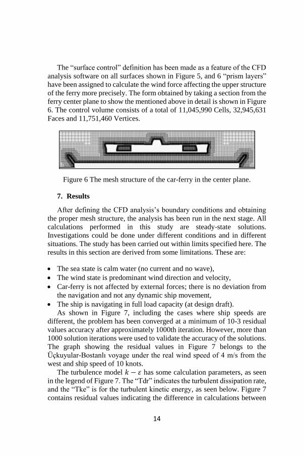
The “surface control” definition has been made as a feature of the CFD
analysis software on all surfaces shown in Figure 5, and 6 “prism layers”
have been assigned to calculate the wind force affecting the upper structure
of the ferry more precisely. The form obtained by taking a section from the
ferry center plane to show the mentioned above in detail is shown in Figure
6. The control volume consists of a total of 11,045,990 Cells, 32,945,631
Faces and 11,751,460 Vertices.
Figure 6 The mesh structure of the car-ferry in the center plane.
7. Results
After defining the CFD analysis’s boundary conditions and obtaining
the proper mesh structure, the analysis has been run in the next stage. All
calculations performed in this study are steady-state solutions.
Investigations could be done under different conditions and in different
situations. The study has been carried out within limits specified here. The
results in this section are derived from some limitations. These are:
The sea state is calm water (no current and no wave),
The wind state is predominant wind direction and velocity,
Car-ferry is not affected by external forces; there is no deviation from
the navigation and not any dynamic ship movement,
The ship is navigating in full load capacity (at design draft).
As shown in Figure 7, including the cases where ship speeds are
different, the problem has been converged at a minimum of 10-3 residual
values accuracy after approximately 1000th iteration. However, more than
1000 solution iterations were used to validate the accuracy of the solutions.
The graph showing the residual values in Figure 7 belongs to the
Üçkuyular-Bostanlı voyage under the real wind speed of 4 m/s from the
west and ship speed of 10 knots.
The turbulence model 𝑘 − 𝜀 has some calculation parameters, as seen
in the legend of Figure 7. The “Tdr” indicates the turbulent dissipation rate,
and the “Tke” is for the turbulent kinetic energy, as seen below. Figure 7
contains residual values indicating the difference in calculations between

15
the two iterations related to RANS equations such as Continuity, X-
momentum, Y-momentum, and Z-momentum.
Figure 7 CFD calculation residual values of the Üçkuyular-Bostanlı
voyage (𝑉𝑠= 10 knots, 𝑉𝑤= 4 m/s west).
According to the technical data of the ferry, it is seen that the maximum
speed is 15 knots. The round-trip voyages with the 1-knot speed intervals
and 9.5 knots service speed have been used for calculations to predict the
added wind resistance of the ship.
A total of 32 analyses have been conducted under 4 m/s wind
conditions, 16 of which are for the Üçkuyular-Bostanlı voyage, and the
remaining belong to the Bostanlı-Üçkuyular. Results of all the performed
analyses are indicated in Table 4 and Table 5. The towing tank resistance
values between 1-6 knots have been derived from test results’ interpolation
between 7-15 knots.
Table 4 CFD analysis results for wind resistance of Üçkuyular-Bostanlı
voyage.
Ship speed
(+x) Real wind speed (m/s)
Apparent wind speed
(m/s) Wind force [N]
knot m/s x axis y axis x axis y axis x axis y axis
15 7.716 1.6269 -3.65 -6.0891 -3.65 -6,504 -19,058
14 7.2016 1.6269 -3.65 -5.5747 -3.65 -5,610 -18,070
13 6.6872 1.6269 -3.65 -5.0603 -3.65 -4,885 -17,102
12 6.1728 1.6269 -3.65 -4.5459 -3.65 -4,228 -15,702
11 5.6584 1.6269 -3.65 -4.0315 -3.65 -3,373 -14,211

16
10 5.144 1.6269 -3.65 -3.5171 -3.65 -2,674 -13,099
9.5 4.8868 1.6269 -3.65 -3.2599 -3.65 -2,431 -12,352
9 4.6296 1.6269 -3.65 -3.0027 -3.65 -2,226 -11,754
8 4.1152 1.6269 -3.65 -2.4883 -3.65 -1,789 -10,981
7 3.6008 1.6269 -3.65 -1.9739 -3.65 -1,220 -10,207
6 3.0864 1.6269 -3.65 -1.4595 -3.65 -757 -9,895
5 2.572 1.6269 -3.65 -0.9451 -3.65 -644 -9,724
4 2.0576 1.6269 -3.65 -0.4307 -3.65 -339 -9,565
3 1.5432 1.6269 -3.65 0.0837 -3.65 -42 -9,576
2 1.0288 1.6269 -3.65 0.5981 -3.65 293 -9,515
1 0.5144 1.6269 -3.65 1.1125 -3.65 508 -9,483
Table 5. CFD analysis results for wind resistance of Bostanlı-Üçkuyular
voyage.
Ship speed
(+x)
Real wind speed
(m/s)
Apparent wind speed
(m/s) Wind force [N]
knot m/s x axis y axis x axis y axis x axis y axis
15 7.716 -1.6269 3.65 -9.3429 3.65 -14,225 25,475
14 7.2016 -1.6269 3.65 -8.8285 3.65 -12,840 24,400
13 6.6872 -1.6269 3.65 -8.3141 3.65 -11,545 23,345
12 6.1728 -1.6269 3.65 -7.7997 3.65 -10,195 22,381
11 5.6584 -1.6269 3.65 -7.2853 3.65 -9,083 21,390
10 5.144 -1.6269 3.65 -6.7709 3.65 -7,914 20,361
9.5 4.8868 -1.6269 3.65 -6.5137 3.65 -7,358 19,838
9 4.6296 -1.6269 3.65 -6.2565 3.65 -6,846 19,315
8 4.1152 -1.6269 3.65 -5.7421 3.65 -5,864 18,367
7 3.6008 -1.6269 3.65 -5.2277 3.65 -5,131 17,356
6 3.0864 -1.6269 3.65 -4.7133 3.65 -4,438 16,186
5 2.572 -1.6269 3.65 -4.1989 3.65 -3,739 14,586
4 2.0576 -1.6269 3.65 -3.6845 3.65 -2,906 13,463
3 1.5432 -1.6269 3.65 -3.1701 3.65 -2,360 12,111
2 1.0288 -1.6269 3.65 -2.6557 3.65 -2,015 11,158
1 0.5144 -1.6269 3.65 -2.1413 3.65 -1,418 10,528
According to the definitions mentioned above, the negative values in the
“𝑥 − 𝑎𝑥𝑖𝑠” column of the wind force values in Table 4 imply the drag force, since the direction of motion of the ship in the direction of +𝑥 for the Üçkuyular-Bostanlı voyage. The negative force values in the “𝑦 −𝑎𝑥𝑖𝑠” column of Table 4 mean that the ship tends to heel towards the starboard side. As in Table 4, for the Bostanlı-Üçkuyular voyage, the ship also navigates in the +𝑥-direction, and the +𝑦-direction indicates the port side of the vessel. Real wind state prevents the ship’s forward motion since all of the wind force values as seen in the “𝑥 − 𝑎𝑥𝑖𝑠” column of Table 5 are negative; also, the “𝑦 − 𝑎𝑥𝑖𝑠” column values enforce the ship to the port side. The fact that ship wind resistance calculations have been

17
achieved from the literature and transformed into an empirical form as equation (12) shows that wind force’s effect on ship resistance cannot be neglected. The added wind resistance forces, that calculated by both CFD and ITTC recommendation, for the Üçkuyular-Bostanlı and Bostanlı-Üçkuyular voyages are shown in Table 6 to compare each other. In this study, only the force component of the wind in the forward direction of the ship, that is, on the 𝑥 − 𝑎𝑥𝑖𝑠, is considered. For this reason, negative ones among the values shown in Table 6 have a slowing effect on the car-ferry, while positive ones do not create added resistance since the ship is in the voyage direction. As shown in Table 7, the bare hull resistance values are indicated as “towing tank resistance” values. As mentioned in Table 2, the results of the towing tank tests performed by (Bal et al., 2014) are the bare hull resistance values used to estimate the case-based total resistance calculations of the ferry used in this study.
Table 6 Comparison of the results of air resistance prediction methods.
Ship speed
(+x)
Üçkuyular-Bostanlı
voyage
Bostanlı-Üçkuyular
voyage Average Average
ITTC
method
CFD
method
ITTC
method
CFD
method
ITTC
method
CFD
method
knot m/s [N] [N] [N] [N] [N] [N]
15 7.716 -3,539 -6,504 -3,539 -14,225 -3,539 -10,364.5
14 7.2016 -3,083 -5,610 -3,083 -12,840 -3,083 -9,225
13 6.6872 -2,659 -4,885 -2,659 -11,545 -2,659 -8,215
12 6.1728 -2,265 -4,228 -2,265 -10,195 -2,265 -7,211.5
11 5.6584 -1,903 -3,373 -1,903 -9,083 -1,903 -6,228
10 5.144 -1,573 -2,674 -1,573 -7,914 -1,573 -5,294
9.5 4.8868 -1,420 -2,431 -1,420 -7,358 -1,420 -4,894.5
9 4.6296 -1,274 -2,226 -1,274 -6,846 -1,274 -4,536
8 4.1152 -1,007 -1,789 -1,007 -5,864 -1,007 -3,826.5
7 3.6008 -771 -1,220 -771 -5,131 -771 -3,175.5
6 3.0864 -566 -757 -566 -4,438 -566 -2,597.5
5 2.572 -393 -644 -393 -3,739 -393 -2,191.5
4 2.0576 -252 -339 -252 -2,906 -252 -1,622.5
3 1.5432 -142 -42 -142 -2,360 -142 -1,201
2 1.0288 63 293 63 -2,015 63 -861
1 0.5144 16 508 16 -1,418 16 -455
Table 7 Total resistance calculations for Üçkuyular-Bostanlı voyage.
Ship speed (+x)
Towing
tank
resistance
(bare hull)
Holtrop-
Mennen
res.
(bare hull)
CFD wind
+ Towing
tank res.
CFD wind /
Towing
tank res.
ratio
Empiric
wind +
Towing
tank res.
Empiric
wind /
Towing
tank res.
knot m/s [N] [N] [N] % [N] %
15 7.716 -122,280 -98,960 -128,784 5.32 -125,819 2.89
14 7.2016 -95,670 -80,044 -101,280 5.86 -98,753 3.22
13 6.6872 -75,190 -63,586 -80,075 6.50 -77,849 3.54
12 6.1728 -57,750 -50,754 -61,978 7.32 -60,015 3.92

18
11 5.6584 -45,980 -40,800 -49,353 7.34 -47,883 4.14
10 5.144 -37,090 -32,800 -39,764 7.21 -38,663 4.24
9.5 4.8868 -33,710 -29,370 -36,141 7.21 -35,130 4.21
9 4.6296 -30,330 -26,250 -32,556 7.34 -31,604 4.20
8 4.1152 -24,810 -20,680 -26,599 7.21 -25,817 4.06
7 3.6008 -19,630 -15,990 -20,850 6.22 -20,401 3.93
6 3.0864 -15,204 -11,935 -15,961 4.98 -15,770 3.72
5 2.572 -12,106 -8,460 -12,750 5.32 -12,500 3.25
4 2.0576 -9,640 -5,560 -9,979 3.52 -9,892 2.61
3 1.5432 -7,676 -3,240 -7,718 0.55 -7,818 1.84
2 1.0288 -6,112 -1,520 -5,819 4.79 -6,049 1.03
1 0.5144 -4,867 -415 -4,359 10.44 -4,851 0.32
All calculations and reference values executed for the Üçkuyular-
Bostanlı voyage in Table 7 are also valid for the opposite voyage (Bostanlı-
Üçkuyular) in Table 8.
Table 8 Total resistance calculations for Bostanlı-Üçkuyular voyage.
Ship speed (+x)
Towing
tank
resistance
Holtrop-
Mennen
res.
CFD wind
+ Towing
tank res.
CFD wind
/ Towing
tank res.
ratio
Empiric
wind +
Towing
tank res.
Empiric
wind /
Towing
tank res.
knot m/s [N] [N] [N] % [N] %
15 7.716 -122,280 -98,960 -136,505 11.63 -125,819 2.89
14 7.2016 -95,670 -80,044 -108,510 13.42 -98,753 3.22
13 6.6872 -75,190 -63,586 -86,735 15.35 -77,849 3.54
12 6.1728 -57,750 -50,754 -67,945 17.65 -60,015 3.92
11 5.6584 -45,980 -40,800 -55,063 19.75 -47,883 4.14
10 5.144 -37,090 -32,800 -45,004 21.34 -38,663 4.24
9.5 4.8868 -33,710 -29,370 -41,068 21.83 -35,130 4.21
9 4.6296 -30,330 -26,250 -37,176 22.57 -31,604 4.20
8 4.1152 -24,810 -20,680 -30,674 23.64 -25,817 4.06
7 3.6008 -19,630 -15,990 -24,761 26.14 -20,401 3.93
6 3.0864 -15,204 -11,935 -19,642 29.19 -15,770 3.72
5 2.572 -12,106 -8,460 -15,845 30.89 -12,500 3.25
4 2.0576 -9,640 -5,560 -12,546 30.15 -9,892 2.61
3 1.5432 -7,676 -3,240 -10,036 30.75 -7,818 1.84
2 1.0288 -6,112 -1,520 -8,127 32.97 -6,049 1.03
1 0.5144 -4,867 -415 -6,285 29.14 -4,851 0.32
8. Conclusion
In this study, a significant difference between the bare hull resistance values calculated by the Holtrop-Mennen method and the towing tank resistance values is observed. Since the hull form of the ferry is a soft multi-chine type, in the empirical resistance prediction equation of Holtrop-Mennen, the effect of the reference ships with the conventional round bilge hull type is seen. The towing tank tests and the CFD analysis are performed with advanced computer technology in such studies as this. Since carrying on the towing tank tests with the wind taken into account is
19
not practicable and feasible, a ship’s total resistance is tried to be calculated by evaluating the superstructure resistance by the CFD analysis.
Within this research scope, wind resistance has been tried to be predicted with CFD analysis, and also, the empirical ITTC formulas are for comparison. It was accepted that the ferry’s average cruising speed is 10 knots, and the predominant wind is blowing from the west direction at a speed of 4 m/s. Direction and velocity magnitudes of apparent wind to be used in CFD and empirical calculations are determined within these assumptions. The average added wind resistance of the round trip of the ship was calculated by CFD method as 14.27% (Bostanlı-Üçkuyular 21.34% and Üçkuyular-Bostanlı 7.21%) of the calm water resistance. According to the ITTC recommendation, this result was calculated as 4.24%. Since the calculation method recommended by ITTC aims to provide preliminary information, the importance of case-based analysis in such cases becomes evident. Besides, since the wind resistance affecting the ship is directly affected by the ship’s superstructure, it has been decided that CFD analysis is necessary for situations where the superstructure, such as the ferry, is considerable.
Considering the financial and environmental impacts of fossil fuel consumption and evolving more restricted rules/regulations enforced by the organizations, it is distinguished that the daily fuel consumption of a ferry, which makes 20 voyages per day and its superstructure is unwieldy compared to other ships, increases by 14.27 percent. Therefore, the aerodynamic resistance calculation of the superstructure of a vessel is vital for shipping operations. It can be concluded that wind tunnel tests have become a necessity in the technical specifications of the container ship, ferry, and car-carrier ships, where the effect of their superstructures on the total resistance is crucial.
The ship’s main engine power’s determination process combines the calm water resistance by using the towing tank tests, empirical formulas, and CFD analysis. The sea margin between 15-30% of the calm water resistance is generally added to a ship’s calm water resistance. Considering the ship’s life cycle, if overall maintenance is not performed correctly, its total performance will deteriorate, which will trigger the vessel not to reach the desired service speed and fuel consumption values. Even if the sea margin is taken into account for calculating the main engine power for the ferry examined in this study as 30%, 14.27% of it will be composed of only wind resistance. As mentioned before, added resistance acting on ships has components such as wave breaking resistance, appendage resistance, roughness resistance, air and wind resistance, steering resistance. This study shows that the added wind resistance calculation with the CFD analysis is crucial that the added sea margin of 30% is not sufficient for this kind of unwieldy ship.
The restrictions mentioned above can be amended with future studies as; route and service speed optimization, sea trial tests for comparison with the study data, and comparing this theoretical study by calculating a 0-10 years old ferry.

20
Acknowledgement
We are thankful for the software support on this study to the Yıldız Technical University, Department of Naval Architecture and Marine Engineering.
References
Bal, Ş., Danışman, D. B., Kanıpek, Z. and Delen, C. (2014). Çift Başlı Feribot Teknesi Model Deneyleri ve Analizi. Istanbul.
Bassam, A. (2017). Use of voyage simulation to investigate hybrid fuel cell systems for marine propulsion.
Birk, L. (2019). Holtrop and Mennen’s Method. In Fundamentals of Ship Hydrodynamics (pp. 611–627). Chichester, UK: John Wiley & Sons, Ltd. https://doi.org/10.1002/9781119191575.ch50
Blendermann, W. (1994). Parameter identification of wind loads on ships. Journal of Wind Engineering and Industrial Aerodynamics, 51(3), 339–351. https://doi.org/10.1016/0167-6105(94)90067-1
Demirel, Y. K. (2012). Yüzey Kirliliğinin Gemi Direnci Üzerindeki Etkisinin İncelenmesi. Fen Bilimleri Enstitüsü, İstanbul. Retrieved from https://polen.itu.edu.tr/handle/11527/4257
Dogrul, A., Song, S. and Demirel, Y. K. (2020). Scale effect on ship resistance components and form factor. Ocean Engineering, 209, 107428. https://doi.org/10.1016/j.oceaneng.2020.107428
Feng, P. Y., Ma, N. and Gu, X. C. (2010). Long-term prediction of speed reduction due to waves and fuel consumption of a ship at actual seas. In Proceedings of the International Conference on Offshore Mechanics and Arctic Engineering - OMAE (Vol. 4, pp. 199–208). Shanghai: American Society of Mechanical Engineers Digital Collection. https://doi.org/10.1115/OMAE2010-20308
Froude, W. (1888). The Resistance of Ships. US Government Printing Office.
Hefny, M. M. and Ooka, R. (2009). CFD analysis of pollutant dispersion around buildings: Effect of cell geometry. Building and Environment, 44(8), 1699–1706. https://doi.org/10.1016/j.buildenv.2008.11.010
Holtrop, J. (1984). A Statistical Re-Analysis of Resistance and Propulsion Data.
Holtrop, J. and Mennen, G. G. (1982). An Approximate Power Prediction Method. International Shipbuilding Progress, 29, 166–170. Retrieved from https://trid.trb.org/view.aspx?id=423662

21
ITTC. (2017). ITTC-Recommended Procedures and Guidelines ITTC-Recommended Procedures and Guidelines Register 0.0 Register.
Kim, M., Hizir, O., Turan, O., Day, S. and Incecik, A. (2017). Estimation of added resistance and ship speed loss in a seaway. Ocean Engineering, 141, 465–476. https://doi.org/10.1016/j.oceaneng.2017.06.051
Korkmaz, S. A. and Cerit, A. G. (2016). Applications of Fuel Cell Technologies in Ships and A System Dynamics Approach. In The Second Global Conference on Innovation in Marine Technology and the Future of Maritime Transportation (pp. 42–56). Muğla-Bodrum.
Larsson, L. and Leif, B. (1990). A method for resistance and flow prediction in ship design.
Lewis, E. V. (Ed.). (1989). Principles of Naval Architecture Second Revision. Jersey: Sname.
Maps, G. (2020). Google maps. Retrieved August 19, 2020, from https://www.google.com/map
Molland, A. F., Turnock, S. R. and Hudson, D. A. (2011). Ship Resistance and Propulsion. Cambridge: Cambridge University Press. https://doi.org/10.1017/CBO9780511974113
Nguyen, T. V., Shimizu, N., Kinugawa, A., Tai, Y. and Ikeda, Y. (2017). Numerical studies on air resistace reduction methods for a large container ship with fully loaded deck-containers in oblique winds. In In MARINE VII: proceedings of the VII International Conference on Computational Methods in Marine Engineering (pp. 1040–1051). CIMNE. Retrieved from https://upcommons.upc.edu/handle/2117/332151
Ozdemir, Y. H., Cosgun, T., Dogrul, A. and Barlas, B. (2016). A numerical application to predict the resistance and wave pattern of KRISO container ship. Brodogradnja: Teorija i Praksa Brodogradnje i Pomorske Tehnike, 67(2), 47–65. https://doi.org/10.21278/brod67204
Schultz, M. P. (2007). Effects of coating roughness and biofouling on ship resistance and powering. Biofouling, 23(5), 331–341. https://doi.org/10.1080/08927010701461974
Seok, J. and Park, J.-C. (2020). Comparative Study of Air Resistance with and without a Superstructure on a Container Ship Using Numerical Simulation. Journal of Marine Science and Engineering, 8(4), 267. https://doi.org/10.3390/jmse8040267
Shigunov, V. (2018). Numerical Prediction of Added Power in Seaway.

22
Journal of Offshore Mechanics and Arctic Engineering, 140(5). https://doi.org/10.1115/1.4039955
Tupper, E. C. (2013). Introduction to naval architecture. Butterworth-Heinemann.
Van He, N., Mizutani, K. and Ikeda, Y. (2016). Reducing air resistance acting on a ship by using interaction effects between the hull and accommodation. Ocean Engineering, 111, 414–423. https://doi.org/10.1016/j.oceaneng.2015.11.023
Windfinder. (2020). windfinder. Retrieved August 19, 2020, from https://www.windfinder.com/#12/38.4244/27.1029/2020-07-11T09:00Z

23
CHAPTER II
VARIOUS INDUSTRIAL APPLICATIONS OF SELF-CLEANING
AND MULTIFUNCTIONAL SURFACES
Ceyda BİLGİÇ
(Assoc. Prof. Dr. ); Eskişehir Osmangazi University, Eskişehir, Turkey
e-mail: [email protected], Orcid No: 0000-0002-9572-3863
Şafak BİLGİÇ
(Asst. Prof. Dr. ); Eskişehir Osmangazi University, Eskişehir, Turkey
e-mail: [email protected], Orcid No: 0000-0002-9336-7762
1. Introduction
After millions of years of slow evolution and natural selection, the
majority of organisms have developed perfect multifunctional surfaces to
adapt to their living environment. In nature, some animals and plants
have a surface with special wettability (Darmanin and Guittard, 2015;
Zhang et al., 2012). For example, lotus leaves grow in the silt but not
imbrued because of their self-cleaning property; (Zorba et al., 2008)
water strider is able to walk and jump on water; (Gao and Jiang, 2004; Hu
et al., 2003) red rose petals show high adhesive force to water droplet and
can capture droplets; (Feng et al., 2008) the rain drops and dew are
inclined to slide along the leaf vein and finally toward the root of a rice
leaf, helping the rice to survive; (Feng et al., 2002; Wu et al., 2011)
butterfly can even fly in the rain because the directional adhesion of the
butterfly wing allows it to shake raindrops off; (Zheng et al., 2007)
mosquito eyes have the antifog ability, ensuring an unimpaired view in
humid conditions where the mosquitoes usually live; (Gao et al., 2007)
desert beetle can harvest fog by its shell in the arid desert; (Parker et al.,
2001) and gecko feet have multifunctions of superhydrophobicity, high
adhesion, and reversible adhesion.
It is found that all of these unique wettabilities are caused by the
combined effect of both different hierarchical surface microstructures and
chemical compositions, verifying the unification and coordination of
structure and performance. Inspired by the above phenomena, a high
amount of artificial functional surfaces with special wettability has been
designed and prepared, and those surfaces have been widely used in our
lives (Tian et al., 2014; Wen et al., 2015; Su et al., 2016; Yong et al.,

24
2015; Yao et al., 2011; Liu et al., 2010). In fact, the study of underwater
superoleophobicity was also originated from the revelation of the antioil
function of fish scales. Compared to the seabirds that are endangered by
oil pollution during a spill accident, fish can keep their body clean in the
same oil-polluted water. In 2009, Liu and co-workers discovered the
underlying mechanism of the antioil ability of fish body, which comes
from the underwater superoleophobicity of the fish scales (Liu et al.,
2009). The fish body is completely covered by well-aligned fan-like
scales. Fish scale is made up of hydrophilic calcium protein, phosphate,
and a thin layer of mucus.
Huang et al, have used multi-scale nano-/micro-roughness structures
to construct self-cleaning surfaces (Huang et al., 2013). The presence of
the hydrophobic silica nanoparticles enables the increase of the water
contact angle. Moreover, the nanoscale roughness reduces adhesion
forces between the water drop and the surface. This phenomenon is
behind the dramatic decrease of the contact angle hysteresis which is
about 85% between smooth particles and particles with nanoscale
roughness. This effect improves the self-cleaning properties. The surface
repellency against liquids with low surface tension should be evaluated to
broaden its application fields (e.g. anti-fingerprint application).
Zhao and Law designed an amphiphobic directional micro-grooved
surface (Zhao and Law, 2012). The as-prepared surface was characterized
by re-entrant morphology and low surface energy. Different wetting
behaviors in the parallel and orthogonal directions to surfaces grooves
were found. Although both directions exhibited amphiphobic property,
the wetting was more favorable in the parallel direction. Besides, liquid
drops were found to be more mobile in the parallel direction (sliding
angles between 4° and 8°) than in the orthogonal direction (sliding angles
between 23° and 34°). The comparison of the anisotropic grooved
surfaces with isotropic patterned pillar structures proved that self-
cleaning is more important in the parallel direction of the grooved
surfaces than in the random pillar arrays. Also, the directional textured
surfaces were expected to be mechanically robust than pillar array
surfaces. These performances are interesting for self-cleaning
applications and robust super-repellency of water and oil.
Huovinen et al. have presented a simple and swift mass fabrication
procedure to produce superhydrophobic and self-clean polymer surfaces
without chemical modification (Huovinen et al., 2012). The prepared
surfaces exhibit higher super-hydrophobicity and superior mechanical
robustness compared to the hierarchical micro-nanostructures. The
mechanical robustness was evaluated by the press and wear tests. The

25
contact angle measured on the micro-microstructure was greater than
150° even after tests, which demonstrates the durability of the super-
hydrophobicity. However, the micro-nano structured surface lost its
super-hydrophobicity after pressure was applied. Such surfaces can be
suitable for anti-fingerprint function since super-hydrophobicity will be
retained after being pressed by a finger. But, wetting behavior against
organic liquids should be studied.
Recently, self-cleaning surfaces have attracted significant attention
since it is highly desirable in many important applications; for example,
since the surface is more wettable to water than to oil, it can be used as a
detergent-free cleaning surface where water can easily replace the oil
contaminants and push the oils away. A Self-cleaning surface can reduce
the consumption of detergents that are made from petroleum. Therefore,
it can save energy and protect the environment from detergent-related
pollution, which are current environmental challenges. It can also be used
as an anti-fogging surface, which is crucial for eyeglasses, camera lenses,
automobiles, and medical instruments such as infrared microscopes
(Howarter and Youngblood, 2007; Howarter and Youngblood, 2008).
This article exemplifies the importance of applications of self-cleaning
and multifunctional materials. Self-cleaning surfaces are becoming an
integral part of our daily life because of their utility in various
applications such as windows, solar panels, cement, paints, etc. Various
categories of materials for the fabrication of hydrophilic, hydrophobic,
oleophobic, amphiphobic, and multifunctional surfaces and their
synthesis routes have been discussed. Furthermore, different natural
organisms exhibiting self-cleaning behavior have been analyzed and the
fundamentals of self-cleaning attributes such as water contact angle,
surface energy, contact angle hysteresis, etc. Self-cleaning surfaces with
excellent water repellence and good mechanical properties are in high
demand. However, producing such surfaces with resistance to mechanical
abrasion and environmental weathering remains a key challenge.
2. Self-cleaning surfaces
Nelumbo nucifera (the lotus plant) is considered to be an embodiment
of purity in Asian religions. The dirt-resistant property of the lotus leaf
has made the researchers investigate its miracle effect in detail.
Randomly distributed micro-papillae of about 5-9 µm in diameter
enclosed by fine nanostructured branches of 120 nm in diameter was
observed. The presence of such surface structures and epicuticular wax
crystalloids made its surface highly superhydrophobic with small sliding
angles. Thus the dirt particles are carried away by the rolling spherical
water droplets, an intrinsic process called self-cleaning or lotus effect.

26
The chemical composition and the geometrical structure of solid surfaces
govern the wettability (Feng et al., 2004). The angle measured through
the droplet at the intervention of three phases - solid, liquid, and vapor, is
referred to as the water contact angle (WCA) (Lafuma and Quere, 2003).
A self-cleaning surface is defined as a surface that is able to keep
itself clean through the natural phenomenon without involving manual
work. The Hydrophobic or hydrophilic phenomenon is the most used
approach for self-cleaning surface treatment (Ragesh et al., 2014).
Hydrophobic surfaces clean the dirt based on the formation of water
droplets that roll away with dirt while hydrophilic surfaces clean the dirt
through the formation of sheeting water that carries away dirt. In recent
years, photocatalysis is also used to photo decompose the contaminants
on the building surface so that the contaminants deposited from the
polluted air change to washable and mineralized compounds (Cassar et
al., 2003).
Since most in-air superoleophobic surfaces usually have
superhydrophobicity, so such superamphiphobic surfaces also have a
self-cleaning ability like ordinary superhydrophobic surfaces. The
concept of the self-cleaning behavior of superamphiphobic surfaces with
low liquid adhesion. Compared with a general surface, the water/oil
droplet on a superamphiphobic surface shows a quasi-spherical shape. If
a water/oil droplet is placed on a slightly tilted superamphiphobic
surface, the droplet can easily roll away. Similar to the lotus leaf having
the self-cleaning ability (Ragesh et al., 2014; Nishimoto and Bhushan,
2013; Yong et al., 2014; Zorba et al., 2008; Zhang, et al., 2012; Ge et al.,
2015) during the Rolling process, the droplet will adhere and remove the
foreign dirt particles on the material surface because it is easier for dust
particles to stick to the liquid droplet than to the solid substrate. In this
way, superamphiphobic surfaces can be kept clean. In contrast, liquid
droplets just pass over the dust on the normally flat surface, leaving the
dust particles behind. Underwater superoleophobic materials with
ultralow oil adhesion also have an excellent self-cleaning function (Wu et
al., 2011; Zhang et al., 2015).
Sun et al. prepared gecko foot-like hierarchical microstructures made
of Polydimethylsiloxane (PDMS) by combining photolithography and
soft lithography (Sun et al., 2008). After subsequent oxygen plasma
treatment, the rough surface showed extreme underwater
superoleophobicity. A soya bean oil droplet was deliberately put onto the
surface as a pollutant in an air environment. The oil quickly adhered and
wetted the sample surface. Interestingly, just by immersing the polluted
sample into the water, the oil was completely removed, whereas the oil

27
on the untreated flat region was still retained; i.e., the oil was not washed
away. This result revealed that underwater superoleophobic surfaces
have a strong self-cleaning ability. Although both the underwater
superoleophobic surface and superhydrophobic lotus leaf have self-
cleaning functions, their self-cleaning abilities are caused by different
physical mechanisms. Water droplets can easily roll away on a lotus leaf
while taking away the dust particles on the leaf (Ragesh et al., 2014;
Yong et al., 2014; Mazumder et al., 2014; Zorba et al., 2008; Zhang et
al., 2012). However, the self-cleaning effect of the underwater
superoleophobic surface originates from its intrinsic superhydrophilicity,
since oil can be removed by the water injection (Nishimoto and Bhushan,
2013). Besides the surface tension of the water/oil/air interface, there is
another main hydrophilic force to push the oil contamination out of the
solid microstructures (Wu et al., 2011). A higher level of hydrophilicity
usually results in a stronger hydrophilic force. Once the oil-polluted
sample is gradually immersed in water, the water is injected into the
rough microstructures and pushes the oil out, resulting in the oil impurity
being cleared.
3. Multifunctional Surfaces
Multifunctional surfaces, as the name suggests have a wide range of
potential applications with a greater degree of control and scalability.
Multiple properties can be encompassed into such surfaces such as
scratch-resistance, self-cleaning property, anti-icing, self-healing, anti-
reflective property, etc. Lee et al. used a simple dip-coating technique to
fabricate multifunctional polymer surfaces in an aqueous solution of
dopamine (Lee et al., 2007). To biomimic the adhesive proteins in
mussels, a thin film of polydopamine was developed using dopamine self
polymerization. These films were used for a range of substrates like
polymers, ceramics, noble metals, oxides, etc. An additional layer could
be deposited using secondary reactions such as electrode-less
metallization for depositing metal films, macromolecule grafting for bio-
inert and bioactive surfaces, etc Wei et al. used oxidant-induced
polymerization to synthesize polydopamine coatings which can be
prepared in acidic/neutral/alkaline aqueous media (Wei et al., 2010). Such
coatings are found to be multifunctional as well as material-independent.
Inspired by the moth eyes which are antireflective and the cicada wings
which are superhydrophobic in nature, Sun et al. tried to biomimic both
these functionalities by fabricating multifunctional optical surfaces (a
template technique) (Sun et al., 2008). Using the soft-lithography process,
fluoropolymer nipple arrays are created which are subwavelength-
structured. The enhancement of both anti-reflective and hydrophobic
functionalities is done by the utilization of fluoropolymers. An

28
experiment and modeling have been done to study the effect of size and
crystalline ordering of the replicated nipples on the antireflective
property. Such surfaces find extensive applications in antireflection self-
cleaning surfaces. Dingremont et al. tried to combine both physical vapor
deposition and nitriding treatment in synthesizing multifunctional
surfaces which made the coating to withstand higher loads, thus
improving their mechanical strength (Dingremont et al., 1995). To
synthesize biomedical surfaces, layer-by-layer assembly finds a great
deal, which is also shown for local drug delivery systems. But such
hydrophobic drugs have a drawback of poor loading capacity
(Dingremont et al., 1995). New synthesis methods have been developed
to combine both oleophobic and hydrophilic characters in coatings to
overcome the limitation of thermodynamic surface energetics. Such smart
surfaces possess different functional groups with favorable and
unfavorable interactions with polar and non-polar liquids, respectively
(Liu et al., 2013). In such smart surfaces, intercalation of oleophobic and
hydrophilic constituents occurs. Oleophobic character is obtained when
the interface, in presence of oil droplets gets occupied by a low-surface
energy component. Nevertheless, due to the hydrophilic components,
water molecules penetrate through such surfaces. Recently spray casting
technique of nanoparticle-polymer suspensions on various substrates was
used to fabricate nanocomposite coatings that encompass both
superhydrophilicity and superoleophobicity (Yang et al., 2012). Such a
dual character is due to the combined cooperation of oleophobic-
hydrophilic groups for hierarchical surface structures. Fluorinated groups
in high surface concentration occupied the interface in the presence of oil
indicating the superoleophobic nature of the surfaces. Due to the surface
molecular re-arrangement induced by water, water molecules could
penetrate through these surfaces. Oleophobic-hydrophilic polymers with
stimuli responses are a great venture for the fabrication of next-
generation anti-fogging and self-cleaning coatings (Howarter and
Youngblood, 2007; Howarter and Youngblood, 2008).
Smart materials like stimuli-responsive polymers on porous materials
are a new attempt for oil/water separation. Inspired by the self-cleaning
lotus effect, Zhang et al. have fabricated polyurethane foam that
encompasses both superhydrophobicity and superhydrophilicity (Zhang
et al., 2013). The as-prepared foam floats easily on water due to its low
density, lightweight, and superhydrophobicity. Multifunctional properties
are demonstrated by the foam-like material in oil/water separation, super-
repellency towards corrosive liquids, and self-cleaning. Such a low-cost
process is promising for the design of multifunctional foams that can be
used for oil-spill clean-up in larger areas.

29
4. Industrial applications of self-cleaning and multifunctional
materials
Inspired by the “lotus effect”, superhydrophobic wetting behavior is
usually used to achieve a self-cleaning surface, which can remain free
from dirt and grime (Nakajima et al., 2000; Fürstner, et al., 2005;
Blossey, 2003). However, most of these surfaces will lose self-cleaning
capability if the surface is ruined with oil contaminants due to its
oleophilicity. To solve this problem, a surface that is more wettable to
water than to oil can be used as the next generation self-cleaning surface
(Howarter and Youngblood, 2008). On this oleophobic/hydrophilic
surface, water itself can wash the oil away and no detergent is required;
therefore, this surface can also be called a detergent-free self-cleaning
surface. Howarter and Youngblood investigated the self-cleaning
capability of simultaneously oleophobic/hydrophilic surfaces (Howarter
and Youngblood, 2007). Oil and water dyed with red color were
sequentially placed on the surface. After a little bit of tilting the substrate,
all the oil droplets were displaced by water and were washed away from
the glass slides. They also performed comparable experiments with
hydrophobic-modified and clean glass slides. The oil droplets stayed on
these two substrates and could not get washed away by water only.
Brown et al. carried out a similar experiment to demonstrate the self-
cleaning capability of glass slide modified with oleophobic/hydrophilic
coating (Brown et al., 2014). Hexadecane on the coated glass slide could
be rinsed away with water, leaving a clean surface. Moreover, Pan et al.
extended the substrate from glass slides to cotton fabrics that are highly
desired for the self-cleaning property in our daily life, and a good self-
cleaning property was observed (Pan et al., 2014).
Self-cleaning surfaces have a large number of applications in
everyday life, agriculture, industry, and military industries. Recently,
many methods and strategies have been used to fabricate self-cleaning
surfaces (Blossey, 2003; Liu and Jiang, 2011; Fürstner et al., 2005).
Many of the self-cleaning coatings such as glasses, tiles, and tissues have
been industrialized. Self-cleaning surfaces could be made using
superhydrophobic surfaces.
The self-cleaning property of the superhydrophobic surface is
necessary to prevent the degradation of efficiency of solar cells because
the snow or dust can easily detach from the surfaces. The
superhydrophobic coating was applied to solar cells with a dimension of
22 x 24 cm by Choi and Huh to investigate the effect of
superhydrophobic surface on light to electricity efficiency of solar cells,
and the results revealed that the short-current densities and open-circuit

30
voltages (Choi and Huh, 2010). The overall enhancement in energy
conversion efficiency of solar cells with the superhydrophobic surface
was about 10% against the solar cells with the normal surface. The self-
cleaning property of the superhydrophobic surface was applied to the
solar cells by Park et al. (Park et al., 2011). The experimental results
revealed that the self-cleaning property of a superhydrophobic surface
was helpful to maintain the efficiency of the solar cells at a high level,
and the efficiency was recovered from 6.56% to 9.78% after the cleaning
process.
Recently, silica substrates were used to construct superhydrophilic
surfaces along with anti-reflective and antifogging properties. The
presence of surface multiscale structures comprising hexagonally non-
close-packed nanonipples covering micro-ommatidia was observed in the
compound eyes of mosquitoes. Soft lithography technique was used to
create an artificial compound eye with superhydrophobicity and anti-
fogging properties that mimic mosquito compound eyes (Gao et al.,
2007). Anti-reflection property is also found in insect wings for
camouflage. Superhydrophobic antireflective self-cleaning properties
were found in the wings of cicada (Lee et al., 2004; Zhang et al., 2006)
Self-cleaning and anti-reflective properties were combined to form so-
called multifunctional optical coatings (Xie et al., 2008; Sun et al., 2008;
Min et al., 2008). Such coatings are used in glass modules for
photovoltaic applications to enhance its efficiency by repelling the dust
and dirt molecules and transmitting almost all the light incident on it.
As the demand for multi-functional materials with special wettability
is increasing, currently, many researchers and engineers are interested in
designing and fabricating superoleophobic surfaces that have a broad
range of applications. Superoleophobic surfaces, both in air and in water,
including anti-oil ability, (Pan et al., 2014; Liu and Jiang, 2011; Liu et al.,
2015) self-cleaning, (Wu et al., 2011; Zhang et al., 2015; Artus, et al.,
2006), oil/water separation, (Xue et al., 2014; Wen et al., 2015; Bixler
and Bhushan, 2014; Zheng et al., 2010; Zhao and Law, 2012; Su et al.,
2016; oil droplet manipulation, (Wu et al., 2011; Zhang et al., 2015; Yong
et al., 2014; Zhang et al., 2013; Kavalenka et al., 2014; Zhang et al.,
2012) chemical shielding, (Pan et al., 2014) anti-blocking, (Wu et al.,
2011; Yong et al., 2014) liquid microlens array, (Lopes et al., 2013) oil
capture, (Cui et al., 2011) bioadhesion, (Su et al., 2016) guiding the
movement of an oil droplet, (Kavalenka et al., 2014; Ragesh et al., 2014)
and floating on oil (Brown, et al., 2014; Ge et al., 2015).
In nature, the lotus leaf can float stably on the water surface, even
with a heavy frog resting on it. The lotus leaf self-cleaning ability, but

31
also enhances its loading capacity; i.e., it is the superhydrophobicity of
the upper surface that endows the lotus leaf with a very large loading
capacity (Yong et al., 2014). The former keeps the lotus leaf clean, while
the latter lets the lotus leaf floating on the water surface and its upper
surface always faces the sky. Both effects benefit its growth by allowing
it to receive more sunlight and maximizing photosynthesis.
5. Conclusions
In this study, recent researches and developments of self-cleaning
surfaces and their applications have been presented. The attractive
properties of self-cleaning surfaces, such as freezing time delay, ice-
accumulation preventing, reducing ice adhesion strength, are discussed.
Durability is one of the most important factors that determine the
practical application of self-cleaning surfaces, which are influenced by
many factors, e.g., temperature and corrosivity. Self-cleaning materials
can find many applications in industries, e.g., using superhydrophobic
surface to retard the frost or ice formation on the surfaces of heat
exchangers and prolong the duration of the ice slurry generation, using
self-cleaning surface to enhance the heat transfer performances of boiling
and condensation, using superhydrophobic/superhydrophilic surfaces for
drag reduction, and so on. Such applications are of positive significance
for energy-saving and performance improvement. Although self-cleaning
surfaces have been subjected to intensive investigations, it is apparent
that further investigations are still necessary for both fundamental and
applicational aspects, for examples, the fabrication process of
superhydrophobic surface needs to be simplified; the durability and
robustness are necessary to be improved for the practical applications; the
fluid flow and heat transfer characteristics and mechanisms on
superhydrophobic/ superhydrophilic surfaces or in the channels with self-
cleaning surfaces are different from those for normal surfaces and both
experimental and theoretical research are indispensable.
Smart self-cleaning surfaces are those which respond to external
influences such as electric field, temperature, light, etc. Researchers are
inspired by nature’s boundless kaleidoscopic effects and they try to
biomimic them to create artificial structures almost close to nature’s
phenomenon. Self-cleaning surfaces basically comprise of hydrophobic
and hydrophilic surfaces. It is already being reflected in our daily life like
the silver nano-coated clothes, waterproof paints, shoes, umbrellas, etc.
Potential coatings that possess various real applications such as
oleophobic surfaces, amphiphobic surfaces, and multifunctional surfaces
have also been studied. The multifunctional surface is an open area where
further research can be motivated. It will find immense applications in the

32
glass industry, medical field (drug-targeting, self-healing), solar cells, etc.
New synthesis and surface modification routes need to be developed
which can provide excellent adhesion and strength for the surfaces on the
substrates used. Other areas of investigation will probably be the study of
the toxicity of such surfaces, so that it can be applied safely in real
applications like water purification membranes, self-repair-, self-healing
and self-lubricating coatings, etc. Even though a large research focus is
going in for the fabrication of such coatings, these synthesis routes need
to be developed which are cost-effective but without compromising the
quality.
Acknowledgments
This study is part of the project (2020-3139) supported by the
Research Fund of Eskişehir Osmangazi University.
References
Artus, G.R.J., Jung, S., Zimmermann, J., Gautschi, H. P., Marquardt, K.,
Seeger, S., (2006), Silicone nanofilaments and their application as
superhydrophobic coatings, Advanced Materials, 18, 2758-2762.
Bixler G.D., Bhushan B., (2014), Rice- and butterfly-wing effect inspired
self-cleaning and low drag micro/nanopatterned surfaces in water, oil,
and air flow, Nanoscale. 2014, 6, 76-96.
Blossey, R., (2003), Self-cleaning Surfaces-Virtual Realities. Nature
Materials, 2, 5, 301-306.
Brown, P.S., Atkinson, O.D.L.A., Badyal, J.P.S., (2014), Ultrafast
oleophobic-hydrophilic switching surfaces for antifogging, self-
cleaning, and oil-water separation, ACS Applied Materials &
Interfaces, 6, 7504-7511.
Cassar, L., Pepe, C., Pimpinelli, N., Tognon, G., Guerrini, G.L., Amadelli,
R., (2003), White cement for architecture concrete, possessing the
photocatalytic properties, in: Proceedings of the 11th International
Congress on the Chemistry of Cement, Durban, 2003, pp.2012-2021.
Choi S.J., Huh S.Y., (2010), Direct structuring of a biomimetic anti-
reflective, selfcleaning surface for light harvesting in organic solar
cells. Macromolecules Rapid Communication, 31(6), 539-544.
Cui, J.P., Zhou, F., Wang, Q.H., Wu, D., Li, D.H., (2011) Transflective
blue phase liquid crystal display using an etched in-plane switching
structure, Journal of Display Technology, 7(7), 398-401.

33
Darmanin, T., Guittard, F., (2015), Superhydrophobic and
superoleophobic properties in nature, Materials Today, 18(5), 273-
285.
Dingremont, N., Bergmann, E., Collignon, P., Michael, H., (1995),
Optimization of duplex coatings built from nitriding and ion plating
with continuous and discontinuous operation for construction and hot
working steels, Surface Coatings Technology, 1995, 72(3), 163-168.
Feng, L., Li, S., Li, Y., Li, H., Zhang, L., Zhai, J., Song, Y., Liu, B., Jiang,
L., Zhu, D., (2002) Super‐hydrophobic surfaces: from natural to
artificial, Advanved Materials, 14, 1857-1860.
Feng, L., Zhang, Y., Xi, J., Zhu, Y., Wang, N., Xia, F., Jiang, L., (2008),
Petal effect: a superhydrophobic state with high adhesive force,
Langmuir, 24, 4114-4119.
Feng, X., Feng, L., Jin, M., Zhai, J., Jiang, L., Zhu, D., (2004), Reversible
Super-hydrophobicity to Super-hydrophilicity Transition of Aligned
ZnO Nanorod Films, Journal of American Chemical Society, 126(1),
62-63.
Fürstner, R., Barthlott, W., Neinhuius, C., Walzel, P., (2005), Wetting and
self-cleaning properties of artificial superhydrophobic surfaces,
Langmuir, 21, 956-961.
Ge, D., Yang, L., Wang, C., Lee, E., Zhang Y., Yang, S., (2015), A multi-
functional oil-water separator from a selectively pre-wetted
superamphiphobic paper, Chemical Communication, 51, 6149-6152.
Gao X., Jiang L., (2004), Biophysics: water-repellent legs of water
striders, Nature, 432, 36-37.
Gao, X., Yan, X., Yao, X., Xu, L., Zhang, K., Zhang, J., Yang, B., Jiang,
L., (2007), The Dry‐Style Antifogging Properties of Mosquito
Compound Eyes and Artificial Analogues Prepared by Soft
Lithography, Advanced Materials, 19(17), 2213-2217.
Hu, D.L., Chan B., Bush, J.W.M., (2003), The hydrodynamics of water
strider locomotion, Nature, 424, 663-666.
Huang, Y.F., Huang, C., Zhong, Y.L., Yi, S.P., (2013), Preparing
superhydrophobic surfaces with very low contact angle hysteresis,
Surface Engeneering, 2013, 29(8), 633-636.
Huovinen, E., Hirvi, J., Suvanto, M., Pakkanen, T.A., (2012), Micro-
micro hierarchy replacing micro-nano hierarchy: a precisely
controlled way to produce wear-resistant superhydrophobic polymer
surfaces, Langmuir, 2012, 28 (41), 14747-14755.

34
Howarter, J.A, Youngblood, J.P., (2007), Self‐Cleaning and Anti‐Fog
Surfaces via Stimuli‐Responsive Polymer Brushes, Advanved
Materials, 19(22), 3838-3843.
Howarter, J.A., Youngblood, J.P., (2008), Self‐Cleaning and Next
Generation Anti‐Fog Surfaces and Coatings, Macromolecules Rapid
Communication, 29(6), 455-466.
Kavalenka, M.N., Hopf, A., Schneider, M., Worgull, M., Hölscher, H.,
(2014), Wood-based microhaired superhydrophobic and underwater
superoleophobic surfaces for oil/water separation, RSC Advances, 4,
31079-31083.
Lafuma, A., Quere, D., (2003), Superhydrophobic States, Nature
Materials, 2, 457-460.
Lee, W., Jin M. K., Yoo, W. C., Lee, J. K., (2004), Nanostructuring of a
polymeric substrate with well-defined nanometer-scale topography
and tailored wettability, Langmuir, 20 (18), 7665-7669.
Lee, H., Dellatore, S.M., Miller, W.M., Messersmith, P.B., (2007),
Mussel-inspired surface chemistry for multifunctional coatings,
Science, 318, 426-430.
Liu, K., Yao, X., Jiang, L., (2010), Recent developments in bio-inspired
special wettability, Chemical Society Review, 39(10), 3240-3255.
Liu K, Jiang L., (2011), Bio-inspired design of multiscale structures for
function integration, Nano Today, 6, 155-175.
Liu, K., Tian, Y., Jiang, L., (2013), Bio-inspired superoleophobic and
smart materials: design, fabrication, and application. Progrees
Material Science, 58(4), 503-564.
Liu, M., Wang, S., Wei, Z., Song, Y., Jiang, L., (2009), Bioinspired design
of a superoleophobic and low adhesive water/solid interface,
Advanved Materials, 21(6), 665-669.
Liu, M., Zheng, Y., Zhai, J., Jiang, L., (2010), Bioinspired super-
antiwetting interfaces with special liquid-solid adhesion,
Accounts of Chemical Research, 43(3), 368-377.
Liu S., Liu X., Latthe, S.S., Gao L., An S., Yoon S.S., Liu B., Xing R.,
(2015) Self-cleaning transparent superhydrophobic coatings through
simple sol-gel processing of fluoroalkylsilane. Applied Surface
Science, 351, 897-903.

35
Lopes, D. M., Ramos, S. M. M., Oliveira, L. R., Mombach, J. C. M.
(2013), Cassie-Baxter to Wenzel state wetting transition: a 2D
numerical simulation. RSC Advances, 3, 24530-24534.
Mazumder, P., Jiang, Y., Baker, D., Carrilero, A., Tulli, D., Infante, D.,
Hunt A.T., Pruneri, V., (2014), Superomniphobic, transparent, and
antireflection surfaces based on hierarchical nanostructures, Nano
Letters, 14, 4677-4681.
Min, W.L., Jiang B., Jiang, P., (2008), Bioinspired self‐cleaning
antireflection coatings, Advanced Materials, 20, 3914-3918.
Nakajima A., Hashimoto K., Watanabe T., (2000), Transparent
superhydrophobic thin films with self-cleaning properties, Langmuir,
16, 7044-7047.
Nishimoto S., Bhushan, B., (2013) Bioinspired self-cleaning surfaces
with superhydrophobicity, superoleophobicity, and
superhydrophilicity, RSC Advances, 3, 671-690.
Pan, S., Guo R., Xu, W., (2014) Durable superoleophobic fabric surfaces
with counterintuitive superwettability for polar solvents, AIChE
Journal, 60(8), 2752-2756.
Park Y.B., Im, H., Im, M., Choi Y.K., (2011), Self-cleaning effect of
highly water-repellent microshell structures for solar cell applications,
Journal of Materials Chemistry, 21(3), 633-636.
Parker, A.R., Lawrence, C.R., (2001), Water capture by a desert beetle,
Nature, 414, 33-34.
Ragesh, P., Ganesh, V.A., Naira, S.V., Nair, A.S., (2014) A review on
‘self-cleaning and multifunctional materials’, Journal of Materials
Chemistry A, 2(36), 14773-14797.
Su, B., Tian, Y., Jiang, L., (2016), Bioinspired Interfaces with
Superwettability: From Materials to Chemistry, Journal of American
Chemical Society, 138(6), 1727-1748.
Sun, C.H., Gonzalez, A., Linn, N. C., Jiang P., Jiang, B., (2008),
Templated biomimetic multifunctional coatings, Applied Physics
Letters, 92, 051107(1-3).
Tian, Y., Su, B., Jiang, L., (2014), Interfaces: Interfacial Material System
Exhibiting Superwettability, Advanced Materials, 26(40), 6872-6872.
Wei, Q., Zhang, F., Li, J., Li, B., Zhao, C., (2010), Oxidant-induced
dopamine polymerization for multifunctional coatings, Polymer
Chemistry, 1, 1430-1433.

36
Wen, L., Tian, Y., Jiang, L., (2015), Bioinspired Super‐Wettability from
Fundamental Research to Practical Applications, Angewande Chemie
International Edition, 54(11), 3387-3389.
Wu, D., Wu, S.Z., Chen, Q.D., Zhao, S., Zhang, H., Jiao, J., Piersol, J.A.,
Wang, J.N., Sun H.B., Jiang, L., (2011), Facile creation of hierarchical
PDMS microstructures with extreme underwater superoleophobicity
for anti-oil application in microfluidic channels, Lab on a Chip, 11,
3873-3879.
Xie, G.Y., Zhang, G.M., Lin, F., Zhang, J., Liu Z.F., Mu, S.C., (2008), The
fabrication of subwavelength anti-reflective nanostructures using a
bio-template, Nanotechnology, 2008, 19, 095605 (1-5).
Xue, Z., Cao, Y., Liu, N., L. Feng L., Jiang, L., (2014), Special wettable
materials for oil/water separation, Journal of Materials Chemistry A,
2, 2445-2460.
Yang, J., Zhang, Z., Xu, X., Zhu, X., Men, X., Zhou, X., (2012),
Superhydrophilic-superoleophobic coatings, Journal of Materials
Chemistry, 22, 2834-2837.
Yao, X., Song, Y., Jiang, L., (2011), Applications of Bio‐Inspired Special
Wettable Surfaces, Advanced Materials, 23(6), 719-734.
Yong, J.L., Yang, Q., Chen, F., Zhang, D., Farooq, U., Du, G., Hou, X.,
(2014), A simple way to achieve superhydrophobicity, controllable water
adhesion, anisotropic sliding, and anisotropic wetting based on
femtosecond-laser-induced line-patterned surfaces, Journal of Materials
Chemistry A, 2, 5499-5507.
Yong, J.L., Chen, F., Yang, Q., Hou, X., (2015), Femtosecond laser
controlled wettability of solid surfaces, Soft Matter, 11, 8897-8906.
Zhang, E., Cheng, Z., Lv, T., Li, L., Liu, Y., (2015), The design of
underwater superoleophobic Ni/NiO microstructures with tunable oil
adhesion, Nanoscale, 7, 19293-19299.
Zhang, G. M., Zhang, J., Xie, G.Y., Liu, Z.F., Shao, H.B., (2006), Cicada
wings: a stamp from nature for nanoimprint lithography, Small, 2,
1440-1443.
Zhang, X., Li, Z., Liu K., Jiang, L., (2013), Bioinspired multifunctional
foam with self‐cleaning and oil/water separation, Advanced
Functional Materials, 23(22), 2881-2886.
Zhang, Y., Chen, Y., Shi, L., Li J., Guo, Z., (2012) Recent progress of
double-structural and functional materials with special wettability,
Journal of Materials Chemistry, 22, 799-815.

37
Zhang, Y.L., Chen, Q.D., Jin, Z., Kim, E., Sun, H.B., (2012) Biomimetic
graphene films and their properties, Nanoscale, 4(16), 4858-4869.
Zhang, Y.L., Xia, H., Kim E., Sun, H.B., (2012), Recent developments in
superhydrophobic surfaces with unique structural and functional
properties, Soft Matter, 8, 11217-11231.
Zhang, Y., Islam, N., Carbonell, R.G., Rojas, O.J., (2013), Specificity and
regenerability of short peptide ligands supported on polymer layers for
immunoglobulin G binding and detection, ACS Applied Materials
Interfaces, 23, 8030-8037.
Zhao H., Law K.Y. (2012), Directional self-cleaning superoleophobic
surface. Langmuir, 28(32), 11812-11818.
Zheng, Y., Guo, X., Jiang, L., (2007), Directional adhesion of
superhydrophobic butterfly wings, Soft Matter, 3, 178-182.
Zheng, J.Y., Feng, J., Zhong, M.Q., (2010), Fabricating superhrdrophilic/
superhydrophobic surfaces bu replica/molding method using CaCO3
particles as, Acta Polymerica Sinica, 10, 1186-2911.
Zorba, V., Stratakis, E., Barberoglou, M., Spanakis, E., Tzanetakis, P.,
Anastasiadis, S.H., Fotakis, C., (2008), Biomimetic Artificial Surfaces
Quantitatively Reproduce the Water Repellency of a Lotus Leaf,
Advanved Materials, 20(21), 4049-4054.

38
CHAPTER III
THERMAL AND STRUCTURAL ANALYSIS OF GEOPOLYMERS
DERIVED FROM INDUSTRIAL WASTE MATERIALS
Ceyda BİLGİÇ
(Assoc. Prof. Dr. ); Eskişehir Osmangazi University, Eskişehir, Turkey
e-mail: [email protected], Orcid No: 0000-0002-9572-3863
Şafak BİLGİÇ
(Asst. Prof. Dr. ); Eskişehir Osmangazi University, Eskişehir, Turkey
e-mail: [email protected], Orcid No: 0000-0002-9336-7762
1. Introduction
Inorganic polymer concretes which are also called “geopolymers”
have arisen an interest in their potential usage in the environmentally
friendly construction and building industry. These materials not only
result in lower greenhouse emissions but also allow the evaluation of raw
clay material sources. Geopolymers display comparable properties to
ordinary portland cement with their robust and versatile technology; the
large scale of raw materials can be used as a source in geopolymerization
so specific properties can be obtained for the desired application (Duxson
et al., 2007:1590). The most commonly used application areas of
geopolymers are; construction and building materials, fire resistance
ceramics, composites, and matrix for immobilization of toxic wastes
(Kumar and Kumar, 2013:865).
Geopolymerisation is a process in which silicon, aluminum, and
oxygen atoms create a chain of SiO4 and AlO4 tetrahedra linked
alternatively by shared oxygen atoms (Wang et al., 2005:1; Davidovits,
1991:1633). The water/solid ratio in this process, if no aggregates are
used, ranges from 0.3 to 0.4 (Xu and van Deventer, 2000:247). The
products are amorphous to semi-crystalline materials with superior
mechanical behavior (Davidovits, 1991:1633; van Jaarsveld et al.,
2002:63; Pacheco-Torgal et al., 2009:200; Tang et al., 2015:1244 ). The
reactants used to form conventional geopolymers are usually industrial
waste materials as the Al-Si source and an activator solution containing
reactive silicate anions and alkali cations (Singh et al., 2004:1943). The
focus of research in this field may be summarised as follows:
i) Al-Si source: identifying low-cost, readily available materials

39
suitable to participate in geopolymerization. It has been shown that a
wide range of natural materials such as Fly ash, slag, and red mud can
be used to make geopolymers.
(ii) alkali activation: analyzing the effects of pH and alkali ions on
process completion and the final properties of the product, e.g. it has
been shown that K-feldspars show increased dissolution in NaOH
solution compared with KOH solution, and thus confer higher
compressive strength (Xu and van Deventer, 2000:247).
(iii) geopolymerization: the mechanisms of the reaction have yet to be
fully understood; the parameters affecting the process, microstructural
reorganization of the source materials, and the reaction steps have
been studied extensively by analytical methods.
The unique properties of geopolymers - high early strength,
extraordinary durability, resistance to chemical attack, ability to
immobilize toxic atoms, and environmental benefits such as low energy
consumption and carbon dioxide emission in production - make
geopolymers a strategic material for sustainable development and a
serious alternative to Portland cement.
Understanding the structure of geopolymers is critical for designing
geopolymers with desired properties. Therefore, this study was
undertaken to review the thermal and structural analysis of the
geopolymers, obtained from the industrial wastes. The samples of
industrial waste and the synthesized geopolymers were characterized by
X-Ray Fluorescence (XRF) for the chemical composition of materials. X-
Ray Diffraction (XRD) measurements are performed to investigate the
amorphous or crystalline phase of the synthesized geopolymers. Fourier
Transform Infrared spectroscopy (FTIR) spectroscopy is utilized to
understand the vibrational fingerprints of geopolymers, Scanning
Electron Microscopy (SEM) images are performed on the synthesized
geopolymers to resolve their surface microstructures. The thermal
degradation and stability of the materials were studied using
thermogravimetric analysis (TGA) and derivative thermogravimetric
analysis (DTG) at several heating rates. The relationships established
between the structure and physical properties will be important for
controlling product properties.
2. Analysis of Geopolymers
2.1. X-Ray Fluorescent (XRF) analysis of geopolymers
X-ray fluorescent (XRF) analysis was carried out to determine the
chemical composition of various binders used in the study of geopolymer

40
and the comparison among the chemical composition of binders can be
seen. Materials such as fly ash, bottom ash, silica fume, rice husk ash,
and others have shown a fair amount of silica and alumina content, which
is suitable to be a substitute as supplementary cementitious materials. The
major oxides present in most of the fly ash samples were mostly silicon
oxide and aluminum oxide. Because ordinary Portland cement was
processed from limestone, it has a higher content in calcium oxide and
silicon oxide but lowers in aluminum oxide. As stated in ASTM C-618,
ashes can be categorized into classes N, F, and C based on the pozzolanic
oxides, namely SiO2, Al2O3, and Fe2O3. According to the listed previous
studies, only ground granulated blast furnace slag and sepiolite contain
less than 50% of pozzolanic oxides. In general, fly ash studied in
previous works fall in class F, which has at least 70% of pozzolanic
oxides except for Abdulkareem et al. (2014) and Embong et al. (2016).
Both studies used Fly ash sourced from the Manjung power plant,
Malaysia which is categorized in class C (Abdulkareem et al., 2014:377;
Embong et al., 2016:816).
2.2. X-Ray Diffraction (XRD) of geopolymers
XRD plays a crucial role in the characterization of geopolymers by
providing information on the crystalline phases and amorphous character
of the samples. Geopolymers are completely amorphous according to X-
ray diffraction (XRD). Typically, they possess a diffuse halo peak at
about 27-30o 2θ (Davidovits, 1991:1633; Lecomte et al., 2003:2571;
Lizcano et al., 2012:2607; Zhang et al., 2005:23). The broad diffuse
hump is corresponding to the amorphous aluminosilicates which form the
primary binder phase in the geopolymer matrix and contribute to the
strength of geopolymers. The angle of this diffuse halo is dependent on
the Si/Al ratio. Increasing Si/Al ratio lowers the degree of the hump
(Lizcano et al., 2012:2607).
The study of geopolymers using X-ray diffraction is difficult because
of the fact, a large part of the structure is amorphous content between 20o
and 40o 2θ. The degree of disorder in geopolymers can be inferred by the
way it diffracts X-ray to form a diffraction pattern. In a non-crystalline
state, diffraction of X-ray results in a broad diffuse halo rather than sharp
diffraction peaks (Davidovits, 1991:1633; Rees et al., 2007:9076). Peaks
were of quartz, mullite, and hematite of the crystalline component of the
fly ash. The broad peak in region 20-30o 2θ arises from the glassy phase
of fly ash and peaks in the region 6-10o and 16o 2θ arise from the
alumino-silicate gel. A considerable amount of zeolites were found in
cement-fly ash system blend, activated by the highly alkaline multi-
compound activator, around pH 14 and cured at 70 oC (Bakharev et al.,

41
2005:1244).
The microstructure of the alkali-activated fly ash changes with the
chemical composition (Rowles et al. 2007:663). After geopolymerization,
all the main characteristic peaks of Al-Si minerals remained but
decreased slightly. This suggested that the Al-Si mineral did not dissolve
totally into the gel phase. However, there were no new peaks, which
means that no new major crystalline phases were formed (Xu and van
Deventer, 2000:247). The baseline broadened between 20o and 40o 2θ
was an indication of an increased amorphicity (van Jaarsveld et al.,
2002:63). Palomo et al. (2014) studied a series of fly ash samples
activated under different experimental conditions and concluded that
geopolymers are a family of materials with the same basic chemical
composition but potentially different microstructures (Palomo et al.,
2014:1). The structural properties of geopolymers depend strongly on
many factors including raw material selection, synthesis conditions,
thermal treatment temperatures, and durations following synthesis and
etc. The phase’s composition and pore structure were characterized by
XRD and SEM.
Abdulkareem et al. (2014), reported a broad hump from 20 o to 35 o
indicating the presence of amorphous geopolymer products
(Abdulkareem et al., 2014:377). Based on previous studies, the presence
of quartz and mullite reflected the composition of typical fly ash. More
than half of the fly ash was composed of iron and calcium. Thus, it
explained the crystalline phases present in the geopolymer paste pattern.
The comparison of the cement-based control sample (CC) with
geopolymer concrete- without the addition of nano-silica shows a wide
hump around 25 o to 35 o in geopolymer concrete with nano-silica. The
intensity of quartz, mullite, and hematite was found higher in geopolymer
concrete with nano-silica due to the presence of additional nano-silica in
the matrix. Some extra peaks are shown in nano-silica modified
geopolymer concrete which indicates the formation of the new phases of
quartz (SiO2), albite (NaAlSi3O8), kaolinite (Al2Si2O5(OH)4), alite
(Ca3SiO5), mullite (3Al2O3∙2SiO2), and Ca(OH)2 crystalline compound
compared to the geopolymer concrete- without the addition of nano-silica
and cement-based control sample. The wide diffraction hump was
detected around 2θ = 25o-35o which confirmed the presence of crystalline
phases in geopolymer concrete with nano-silica. As discussed earlier,
crystalline phases were exposed after the addition of alkaline solution.
Zeolite was formed after the dissolution while mullite, quartz, and
hematite exist in all fly ashes.

42
Tho-In et al. (2018) reported the XRD analysis at the age of 7-day of
Fly ash-based geopolymer paste with ground container glass (Tho-In et
al., 2018:2892). The Fly ash-based geopolymer paste has a wide hump at
25 o to 35 o and low phases of calcite that corresponds to the high degree
of geopolymerization (Phoo-ngernkham et al., 2014:58). The XRD trends
of Fly ash-based geopolymer paste with ground container glass pastes are
similar to that of Fly ash geopolymer paste. However, peaks of quartz and
calcite were observed as the percentage of ground container glass
increased due to the high contents of SiO2 and CaO (Wongsa et al.,
2017:49). Peaks of cristobalite and tridymite were noted at a higher
percentage with ground container glass replacement.
Ground granulated blast furnace slag-based geopolymer represented the
development of phases of geopolymer from early age to long-term
specimen. The high-intensity peak, 2θ for 28 days geopolymer paste is
reported at 27o. Many minerals from bauxite ore tailing such as
corundum, muscovite, anatase, quartz, and mullite are still identified for
the long-term specimen. However, the formation of calcite mineral is
detected in the long-term specimens which hinted the specimen is
susceptible to carbonation ( Ye et al., 2017:23).
The chemical composition of geopolymer is similar to zeolitic
materials. Sometimes, geopolymers are regarded as a zeolitic precursor.
The difference between geopolymers and zeolites is that geopolymer is
amorphous, whereas zeolite is crystalline in nature (Lecomte et al.,
2003:2571; Khale and Chaudhary, 2007:729). Crystallization does not
only depend on curing temperature but also influenced by the type of
alkali reactant used and curing time. Zeolite crystallization is promoted
by high water content, high curing temperature as well as extended curing
period (Provis et al., 2005:3075). Zeolite crystallites are also increasing
with aging (Duxson et al., 2007:8).
It is known that zeolites are highly porous and have poor mechanical
properties. It was believed that there is always a limitation of the amount
of crystalline phase that can be tolerated by the matrix. Several
researchers (Kolousek et al., 2007:9267; Palomo et al., 1999:997)
discovered that zeolite crystallites reinforce the geopolymer matrix and
improve strength, but it will cause a substantial reduction in long-term
strength. A similar strength development trend has been concluded for fly
ash geopolymers (Criado et al., 2007:671).
2.3. Scanning Electron Microscope (SEM) of geopolymers
Scanning Electron Microscopy (SEM) can be used to study the
morphology of raw materials and synthesized of raw material-based

43
geopolymers. Micromorphologies of geopolymers, fast and non-
destructive technique gives information about surface properties, particle
size and also particle distribution (Yunsheng et al., 2010:271). Differ
from metakaolin geopolymers; fly ash geopolymers reveal heterogeneous
elements with lots of unreacted fly ash particles in the hollow cavities left
by the partially dissolved fly ash particles. Unreacted particles act as a
filler and strengthen the composite. In fly ash geopolymers, smooth and
connecting geopolymer matrix was observed instead of a globular unit of
geopolymer matrix in metakaolin geopolymers.
Many researchers reported on fly ash-based geopolymer concrete with
variables that include additional binders, alkali activator ratio, molarity,
and curing temperature & duration (Assi et al., 2016:806; Pavithra et al.,
2016:117; Xie and Ozbakkaloglu, 2015:5945). Pavithra et al. (2016)
researched fly ash-based geopolymer concrete and suggested a method as
explained here to obtain optimum mix design (Pavithra et al., 2016:117).
A few parameters such as molarity, sodium silicate to sodium hydroxide
ratio (SS/SH), curing temperature, and duration was set as constant
variables before deciding for the alkaline activator solution (AAS). In this
study, the authors suggested that the water content to be used relied on
the maximum aggregate size, as it can be used to control the limit of
maximum water content. Calculation on binder content, alkaline activator
solution, water content, the fine, and coarse aggregate was carried out
based on the priority of the mix whether strength or alkaline activator
solution to binder ratio is to be focused on. The effect of different alkaline
solution-to-binder contents on the microstructure of geopolymer concrete
was compared. The precipitation decreases constantly as the ratio of
alkaline activator solution /binder increases. It is understood that as this
ratio increases, the strength of geopolymer concrete decreases due to the
increasing amount of water present in the geopolymer mix. This
phenomenon is comparable with ordinary Portland cement concretes with
a higher water/cement ratio. The contact area for the reaction was blocked
by the water molecules and this, in turn, affected the geopolymerization
process between the binder and the activator; this resulted in low
compressive strength of geopolymer concrete (He et al., 2011:59). With
appropriate alkali activator/binder ratios of 0.4 and 0.5, the unreacted Fly
ash particles were found minimum. Also, the number of voids is sparse.
The fineness of fly ash also contributed to the dense matrix, which helps
reduce the formation of microcracks. Apart from that, the strength of
geopolymers was improved fairly due to the ability of fly ash to fill the
microcracks, which is in line with the study of Xie and Ozbakkaloglu
(2015) and Assi et al. (2016) (Assi et al., 2016:806; Xie and
Ozbakkaloglu, 2015:5945).

44
The effect of different mass ratios of sodium silicate to sodium
hydroxide of fly ash-based geopolymer was studied through micro-
structural investigation by Abdulkareem and Ramli (2015) (Abdulkareem
and Ramli, 2015:61). Fully reacted fly ash was observed for geopolymer
with alkaline activator mass ratios of 0.5 and 1.0. Even though a similar
microstructure was observed for both mass ratios of 0.5 and 1.0, the
compressive strength obtained for the mass ratio of 1.0 was 65 MPa
compared to 35 MPa for the mass ratio of 0.5. Supported by the previous
study, a higher concentration of silicate might contribute to higher
strength development due to more silicates available for
geopolymerization (Palomo et al., 1999:1323). However, the comparison
shows that a higher mass ratio of sodium silicate resulted in unreacted fly
ash particles. The use of activator mass ratios of 2.0 and 3.0 displayed
high content of unreacted and partially reacted fly ash microspheres. It is
understood that too much alkaline activator solution in the mix hampered
the process of geopolymerization by limiting the interaction between the
binder and alkaline activator solution (Villa et al., 2010:2084). Besides,
geopolymer samples with SS/SH mass ratio of 3.0 recorded the weakest
compressive strength of 32 MPa. The comparison of recent studies on
this subject shows that most of the authors used the mass ratio of SS/SH
up to 2.5 (Okoye et al., 2016:3000; Xie and Ozbakkaloglu, 2015:5945;
Noushini et al., 2016:136). While another study has produced similar
properties of geopolymer with a higher mass ratio of alkaline solution,
the curing temperature might have been contributed to the dense structure
(Gunasekara et al., 2016:352). Curing temperature of 70 oC or higher
tends to have a looser arrangement due to evaporation of free water
which causes continuous microcracks within the matrix; (Kong and
Sanjayan, 2010:334; Chindaprasirt et al., 2007:224). According to
Chindaprasirt et al. (2007), an adequate amount of water is necessary for
the process of geopolymerization to have high strength development
(Chindaprasirt et al., 2007:224). Okoye et al. (2016) examined the
microstructure of geopolymer made of fly ash and silica fume (Okoye et
al., 2016:3000). In contrast with previous studies, a geopolymer concrete
sample with fly ash was found to have a fracture surface. The observation
of voids proved a loose arrangement of particles. Whereas smoother
surface was observed for the 20 % replacement of fly ash with silica fume
in the fly ash-based geopolymer concrete.
SEM images of pure geopolymer and geopolymer nanocomposites
containing 3.0 wt% nano-silica in wet and dry mix conditions. A
significant amount of unreacted and partially reacted fly ash particles was
observed in the case of pure geopolymer. However, the number of
unreacted particles decreased. Besides, microcracks observed using the

45
dry mix procedure, are lower than the pure geopolymer and wet mix.
Unlike Pavithra et al. (2016), the microstructure of bottom ash and fly ash
in geopolymer was studied by Xie and Ozbakkaloglu (2015) (Pavithra et
al., 2016:117; Xie and Ozbakkaloglu, 2015:5945). As the mass ratio of
fly ash to bottom ash increases, the strength of the sample increases, too.
The presence of bottom ash, however, reduced the strength of
geopolymer and it could be attributed to the larger surface area of bottom
ash with the presence of foreign objects that failed to react fully in the
geopolymer.
A small number of semi-spheres was present along with some
rectangular-shaped objects. While the composition test revealed the
presence of foreign object-radium, a radioactive earth metal in the bottom
ash, there were no foreign objects nor irregular-shaped particles found in
fly ash. Other than the presence of foreign objects, some of the bottom
ash did not react fully in the process of geopolymerization and this
contributed to lower compressive strength compared to pure fly ash-based
geopolymer. Similar to previous studies, unreacted Fly ash residues were
observed that only small traces of sodium element were observed on the
non-reactive minerals covering the unreacted Fly ash particles (Xie and
Ozbakkaloglu, 2015:5945; Embong et al., 2016:816). Due to the low
calcium content present in Gaston Fly Ash, insignificant amount of
calcium element, SEM image illustrated that crystalline phases were
exposed, and new precipitant was formed after the dissolution of Gaston
Fly Ash using an alkaline solution. After the dissolution, parts A, B, and
C correspond to zeolite, mullite, and hematite (Zeng and Wang,
2016:386).
Sharmin et al. (2017) has utilized a high volume of ground granulated
blast furnace slag (GGBS) along with metakaolin (MK) and rice husk ash
(RHA). A continuous compact microstructure is observed for the
optimum mix (0.25:0.25:0.50 for MK: RHA: GGBS). It is understood
that mixes with high volume GGBS used to replace RHA, has
subsequently improved the compressive strength. Utilize high volume of
RHA is known for geopolymer with lower compressive strength and
more brittle due to the larger solid particle and lower specific gravity of
RHA (Chindaprasirt et al., 2007:224; Sharmin et al., 2017:608).
Additional MK in geopolymer was able to contribute stronger Si-O-Al
and Al-O-Al bonds than the Si-O-Si bond. However, the utilization of a
high volume of MK is not advisable as it will produce sodium alumina
silicate (zeolite) (Duxson et al., 2005:47). Zeolite is known for its
negative effect on strength development as a result of excess alumina
from MK. Subsequently, the process of polymerization is hindered as a

46
high concentration of the alkaline activated solution was required to
activate a high volume of MK. Thus, the usage of MK in geopolymer
needs appropriate consideration for achieving desired results. Ye et al.
(2017) studied the early age and long-term microstructure of bauxite ore
tailing and slag-based geopolymer paste. The microstructure of 28-days
where porous gel with noticeable large pores was observed. It was
predicted that the continuous geopolymerization process has been able to
produce the gels where large pores tend to reduce in small and volume for
a long-term specimen. The linking of geopolymer gels has formed
capillary gels in pores and cracks (Ye et al., 2017:23).
Structural characterization was also performed using Scanning
Electron Microscopy with Energy Dispersive X-Ray (SEM-EDX)
analysis. In addition to SEM micrographs and EDX spectroscopies, an
elemental mapping was done to some of the samples of the 1st category to
inspect the effect of the studied parameters on the elemental distribution
of the manufactured samples and thereby obtain an evaluation of the
matrix through the ratios of the elements. The elemental mapping
revealed the fact that in general a homogeneous distribution of the
elements was observed. The observations are considered in line with the
obtained results and the micrographs of the samples.
The SEM micrographs and the EDX spectroscopies of the main mixes
were taken. As a general observation, the micrographs of the investigated
samples indicate a satisfactory degree of compactness and good
microstructural bonding between the components of the geopolymeric
matrix. Some unreacted fly particles were observed in the micrographs,
the existence of unreacted particles is an indicator of a good strength
behavior because these particles will affect positively the bonding pattern
of the manufactured samples (Sung et al., 2013:409).
2.4. Fourier Transform Infrared Spectroscopy (FTIR) of
geopolymers
FTIR spectra of geopolymers is generally characterized by broadband
in the 900-1300 cm-1 region that is characteristic of disordered
geopolymer structure. Bands observed in this region are related to
asymmetric stretching vibrations of Si–O–T (T=Al, Si) ( Ye et al.,
2014:1652; Arıöz et al., 2012:1115). The shift of this band to lower
wavenumbers is a clear indication of the dissolution of the raw materials
in an alkaline activator and the evolution of a new amorphous
aluminosilicate phase during the geopolymerization process. Similar
results are obtained in the study where FTIR spectroscopy is performed
on fly ash-based geopolymers. FTIR band detected at 1085 cm-1 in fly ash
has shifted to lower frequencies (986 cm-1) with alkaline activation (Arıöz

47
et al., 2012:1115). Bands detected in the region between 550 - 750 cm-1
are assigned to symmetric stretching vibrations of Si–O–Si and Al–O–Si.
An enhancement in the intensity of the bands in this region points out an
enhancement in chain length and formation of aluminosilicate gel. High-
frequency bands observed in the region between 1300-1600 cm-1 are
assigned to stretching vibrations of O–C–O bonds and show the presence
of carbonate materials (Ye et al., 2014:1652; Dimas et al., 2009:211;
Mustafa Al Bakri et al., 2011:289). In a recent study, red mud is used
together with fly ash as a raw material for geopolymer production, and a
peak is detected at 458 cm-1 (Kumar and Kumar, 2013:865), this peak is
associated with vibrations of Fe–O bonds (Muñiz-Villarreal et al.,
2011:995) because of the iron present in red mud. Band detected at
frequencies higher than 1600 cm-1 is due to stretching (–OH) and bending
(H–O–H) vibrations of interlayer adsorbed H2O molecules (Nath and
Kumar, 2013:924; Mustafa Al Bakri et al., 2011:289). In a recent research
employing fly ash and bottom fly ash in geopolymer production, FTIR
spectra of raw materials and products are used to quantitively express the
degree of geopolymerization. This calculation is made in terms of height
ratios and area ratios of the Si–O–Si stretching peaks that exist in the
FTIR spectra of geopolymers to their regarding ashes’ peak. It is found in
this study that the ratios of peak heights and areas to their corresponding
ashes are much higher and this situation points out the high degree of
geopolymerization in the system (Ferone et al., 2013:1920).
A FTIR analysis for Fly ash-based geopolymer was carried out by
Adak et al. (2017) to determine the structure of geopolymer (Adak et al.,
2017:430). The distinct intensity band near 460 cm-1 was recognized for
the Si–O–Si bending vibration. The band between 750 cm-1 and 800 cm-1
was observed due to the AlO4 vibration. Another peak for the asymmetric
stretching and vibration band of Si–O–T (T = Al, Si) which was described
as the strongest band, registered in the region of 950 cm-1 -1050 cm-1. The
position (1420 cm-1 ) of Si–O–Si in with geopolymer concrete- without
the addition of nano-silica was shifted to the right position (1485 cm-1 ) in
geopolymer concrete with nano-silica. A significant band was also
located at approximately 3450 cm-1 for OH stretching bonding.
Tho-In et al. (2018) conducted the FTIR analysis on Fly ash-based
geopolymer with ground fluorescent lamp (FP) and container glass pastes
(Tho-In et al., 2018:2892). The absorption bands at approximately 3450
cm-1 and the weak band 1650 cm-1 are associated with the vibrations of
O–H and H–O–H bonds in the water molecules. Previous studies reported
that the bands as reported by Tho-In et al. (2018) revealed that the water
molecules were absorbed on the surface or embedded in the pores during
the process of geopolymerization (Tho-In et al., 2018:2892; Fernández-

48
Jiménez and Palomo, 2005:1984). The band at roughly 1450 cm-1
indicated the extension of O–C–O in carbonate groups due to the reaction
of alkali metal hydroxides with atmospheric CO2 (Panias et al.,
2007:246). The irregular stretching of Si–O–X bonds found in all
specimens is located at 1050 cm-1, where X representing tetrahedral
silicon or aluminum atom. The Si–O–X bond supported the
geopolymerization process with the phases of amorphous
aluminosilicates formed. Besides, researchers also stated that the sharp
absorption band correlates to the number of tetrahedrally coordinated
aluminum that exists in the geopolymer gel (Gao et al., 2014:503).
Furthermore, the stretching of O–Si–O and Si–O–Si bonds which can be
located at 450 cm-1 is identical to those Si–O–Al groups (Zawrah, et al.,
2016:237).
2.5. Thermogravimetric Analysis of geopolymers
Information about the thermal stability of the samples and the weight
loss versus temperature changes is measured by thermogravimetric
analysis (TGA) and differential thermogravimetric analysis (DTGA).
TGA is performed using TA instruments and the analysis is done by using
nitrogen at a flow rate. The characteristic subsequent phases observed in
the thermogravimetric analysis of geopolymers are; i) dissipation of free
water molecules, ii) decomposition of geopolymer components, iii)
dehydroxylation of zeolitics, iv) stabilization of the weight (Cheng et al.,
2015:74).
Thermal analysis was carried out by Abdulkareem et al. (2014) to
measure the mass loss as a function of temperature from 25 oC to 800 oC.
Thermogravimetric analysis (TGA) and the derivative thermogravimetric
analysis (DTG) curves for the geopolymer paste were displayed. Loss of
water due to evaporation of both the free and some of the chemically
bonded water from geopolymer was demonstrated with a decrease in
mass rapidly before 150 oC (Abdulkareem et al., 2014:377). Roughly 55-
60% of free water present in the geopolymer matrix evaporated before
100oC in samples was illustrated by the sharp weight loss. However, it is
observed that the rate of weight loss stabilized from 150°C to 780°C, on
account of the evaporation of chemically bonded water and the hydroxyl
groups, –OH. No further mass loss was detected with the increase of
temperature to 800°C. The average mass after heated to 800°C was
79.8%.
Kong and Sanjayan (2010) analyzed the behavior of Fly ash-based
geopolymer paste under elevated temperature (Kong and Sanjayan,
2010:334). Withstanding with Abdulkareem et al. (2014) the sharp weight
loss came at 250oC instead of 150oC, which is also attributed to the

49
evaporation of the hydroxyl group (Abdulkareem et al., 2014:377;
Duxson et al., 2005:47). The change in weight is rather constant after 300 oC. Kong and Sanjayan (2010) hypothesize that the slow rate of thermal
shrinkage recorded from 300 oC and above is associated with the low rate
of weight loss (Kong and Sanjayan, 2010:334). The average mass
recorded after 800oC exposure was 89%. Duan et al. (2016) studied the
thermal analysis of geopolymer paste with iron ore tailing (IOT) (Duan et
al., 2016:600). The content of calcium hydroxide Ca(OH)2 decreased
when the content of iron ore tailing increased, which was attributed to the
lesser mass loss compared to the reference sample. It is understood that
the addition of iron ore tailing contributed to the formation of calcium
silicate hydrate by utilizing Ca(OH)2. Nevertheless, even after 30% of
iron ore tailing was added to the mix, the decomposition of Ca(OH)2
recorded corresponding to the endothermic peak. It was reported that
Ca(OH)2 still presents as only a number of the calcium was converted
into calcium silicate hydrate. Similar to Abdulkareem et al. (2014), the
rate of mass loss at high temperatures after 800oC was negligible for all
samples (Abdulkareem et al., 2014:377). Thermal analysis was conducted
by Okoye et al. (2016) to study the thermal stability of geopolymers
(Okoye et al., 2016:3000). The weight loss for both kaolin incorporated
Fly ash-based geopolymer and pure Fly ash-based geopolymer samples
took place at approximately 100 oC. For the Fly ash-based geopolymer, a
rather sharp drop in weight was observed when temperature increased
whereas the kaolin incorporated -based geopolymer has a complex curve.
From the observation of both samples, the ideal curing temperature could
be ranged from 80oC to 100oC.
3. Conclusions
Innovative technology studies have started to focus on ‘geopolymers’
that are inorganic polymers that arise as potential future alternatives to
cement-based materials. Geopolymer was first used as a fire-resistant to
protect cruise ships from fire, in the protection of wooden structures, and
different implementations. Geopolymers have also been shown to display
good mechanical and thermal properties, low shrinkage, and longer
design lives compared to some cementitious materials. Geopolymers, if
used as an alternative to Portland cement, CO2 emission produced by
geopolymer technology is estimated to be 80% less than Portland cement.
Therefore, it is thought that geopolymer technology is going to be vital in
the near future for the green construction industry.
This study offers insights into the various techniques used for the
characterization of geopolymers derived from industrial waste materials.
Understanding the structure of geopolymers is critical for designing

50
geopolymers with desired properties. The relationships established
between the structure and physical properties will be important for
controlling product properties.
Acknowledgments
This study is part of the project (2018-2233) supported by the
Research Fund of Eskişehir Osmangazi University.
References
Abdulkareem O.A., Mustafa Al Bakri A.M., Kamarudin H., Khairul Nizar
I., Saif A.A., (2014) Effects of elevated temperatures on the thermal
behavior and mechanical performance of fly ash geopolymer paste,
mortar and lightweight concrete. Construction and Building
Materials, 50, 377-387.
Abdulkareem, O.A., Ramli, M. Optimization of alkaline activator mixing
and curing conditions for a fly ash-based geopolymer paste system,
Modern Applied Science, 9 (12) (2015) 61-69.
Adak, D., Sarkar, M., Mandal, S. (2017) Structural performance of nano-
silica modified fly-ash based geopolymer concrete, Construction and
Building Materials, 135 (2017) 430-439.
Assi L., Ghahari S.A., Deaver E.E., Leaphart D., Ziehl P. (2016)
Improvement of the early and final compressive strength of fly ash-
based geopolymer concrete at ambient conditions, Construction and
Building Materials, 123, 806-813.
Arıöz, E., Arıöz, Ö., Koçkar, Ö.M. (2012) “Leaching of F-type Fly Ash
Based Geopolymers’’, 20th International Congress of Chemical and
Process Engineering CHISA, Procedia Engineering, 42, 1114-1120.
Bakharev T. (2005) “Geopolymeric materials prepared using Class F fly
ash and elevated temperature curing” Cement and Concrete Research,
35(6),1224-1232.
Cheng, H., Lin, K.L., Cui, R., Hwang, C.L., Cheng, T.W., Chang, Y.M.
(2015) “Effect of Solid-to-Liquid Ratios on the Properties of Waste
Catalyst-Metakaolin Based Geopolymers”, Construction and Building
Materials, 88, 74-83.
Chindaprasirt, P., Chareerat, T., Sirivivatnanon, V. (2007) Workability and
strength of coarse high calcium fly ash geopolymer, Cement and
Concrere Composites, 29 (3), 224-229.
Criado M., Fernández-Jiménez A., de la Torre A.G., Aranda M.A.G.,

51
Palomo A. (2007) An XRD study of the effect of the SiO2/Na2O ratio
on the alkali activation of fly ash, Cement and Concrete Research,
37(5), 671-679.
Davidovits, J. (1991) ‘‘Geopolymers: Inorganic Polymeric New
Materials’’, Journal of Thermal Analysis and Calorimetry, 37(8),
1633-1656.
Dimas, D. D., Giannopoulou, I.P., Panias, D. (2009) ‘‘Utilization of
Alumina Red Mud for Synthesis of Inorganic Polymeric Materials’’,
Mineral processing and extractive metallurgy review: An International
Journal, 30 (3), 211-239.
Duan P., Yan C., Zhou W., Luo W. (2016) Fresh properties, mechanical
strength and microstructure of fly ash geopolymer paste reinforced
with sawdust, Construction and Building Materials, 111, 600-610.
Duxson, P., Provis, J.L., Lukey, G.C., Mallicoat, S.W., Kriven, W.M., Van
Deventer, J.S.J. (2005) “Understanding the Relationship Between
Geopolymer Composition, Microstructure and Mechanical
Properties”, Colloids and Surfaces A: Physicochemical and
Engineering Aspects, 269 (1-3), 47-58.
Duxson P, Mallicoat, S.W., Lukey, G.C., Kriven W.M., van Deventer J. S.
J. (2007), The effect of alkali and Si/Al ratio on the development of
mechanical properties of metakaolin-based geopolymers, Colloids
and Surfaces A: Physicochemical and Engineering Aspects, 292(1), 8-
20.
Duxson P., Provis J.L., Lukey G.C., van Deventer J. S. J. (2007) ‘‘The
Role of Inorganic Polymer Technology in the Development of 'Green
Concrete'’’, Cement and Concrete Research, 37(12), 1590-1597.
Embong, R., Kusbiantoro, A., Shafiq, N., Nuruddin, M.F. (2016) Strength
and microstructural properties of fly ash based geopolymer concrete
containing highcalcium and water-absorptive aggregate, Journal of
Cleaner Production, 112, 816-822.
Ferone, C., Colangelo, F., Roviello, G., Asprone, D., Menna, C., Balsamo,
A., Prota, A., Cioffi, R., Manfredi, G. (2013), “Application-Oriented
Chemical Optimization of a Metakaolin Based Geopolymer’’,
Materials, 6(5), 1920-1939.
Fernández-Jiménez, A., Palomo, A. (2005) “Composition and
Microstructure of Alkali Activated Fly Ash Binder: Effect of the
Activator”, Cement and Concrete Research, 35(10), 1984-1992.
Gao K., Lin K.L., Wang D.Y., Hwang C.L., Shiu H.S., Chang Y.M.,

52
Cheng T.W. (2014), Effects SiO2/Na2O molar ratio on mechanical
properties and the microstructure of nano-SiO2 metakaolin-based
geopolymers, Construction and Building Materials, 53, 503-510.
Gunasekara, C., Law, D.W., Setunge, S. (2016) Long term permeation
properties of different fly ash geopolymer concretes, Construction and
Building Materials, 124, 352-362.
He P., Jia D., Wang M., Zhou Y. (2011) Thermal evolution and
crystallization kinetics of potassium-based geopolymer, Ceramics
International, 37 (1), 59-63.
Khale D., Chaudhary R. (2007) “Mechanism of geopolymerization and
factors influencing its development: a review”, Journal of Materials
Science, 42, 729-746.
Kolousek D., Brus J., Urbanova M., Andertova J., Hulinsky V., Vorel J.
(2007) “Preparation, structure and hydrothermal stability of alternative
(sodium silicate-free) geopolymers”, Journal of Materials Science,
42(22), 9267-9275.
Kong D.L.Y., Sanjayan, J.G., (2010) Effect of elevated temperatures on
geopolymer paste, mortar and concrete, Cement and Concrere
Research, 40 (2), 334-339.
Kumar, A., Kumar S. (2013) “Development of Paving Blocks from
Synergistic Use of Red Mud and Fly Ash Using Geopolymerization”,
Construction and Building Materials, 38, 865-871.
Lecomte I., Liegeois M., Rulmont A., Cloots R., (2003) “Synthesis and
characterization of new inorganic polymeric composites based on
kaolin or white clay and on ground-granulated blast furnace slag”,
Journal of Materials Science, 18(11), 2571-2579.
Lizcano M., Kim H.S., Basu S., Radovic M. (2012) Mechanical
properties of sodium and potassium activated metakaolin-based
geopolymers. , Journal of Materials Science, 47, 2607-2616.
Mustafa Al Bakri, A.M., Kamarudin H., BinHussain M., Khairul Nizar I.,
Zarin Y., Rafiza A.R. (2011) “The Effect of Curing Temperature on
Physical and Chemical Properties of Geopolymers’’, Physics
Procedia, 22, 289-290.
Muñiz-Villarreal, M. S., Manzano-Ramírez, A., Sampieri-Bulbarela, S.,
Ramón Gasca-Tirado J., Reyes-Araiza, J.L., Rubio-Ávalos, J.C.,
Pérez-Bueno, J.J., Apatiga, L.M., Zaldivar-Cadena A., Amigó-Borrás
V. (2011) “The Effect of Temperature on the Geopolymerization
Process of a Metakaolin-Based Geopolymer’’, Materials Letters,
53
65(6), 995-998.
Nath S. K., Kumar, S. (2013) “Influence of Iron Making Slags on
Strength and Microstructure of Fly Ash Geopolymer”, Construction
and Building Materials, 38, 924-930.
Noushini A., Aslani F., Castel A., Gilbert R.I., Uy B., Foster S. (2016)
Compressive stress-strain model for low-calcium fly ash based
geopolymer and heat-cured Portland cement concrete, Cement and
Concrere Composites, 73, 136-146.
Okoye, F.N., Durgaprasad, J., Singh, N.B. (2016) Effect of silica fume on
the mechanical properties of fly ash based-geopolymer concrete,
Ceramics International, 42 (2), 3000-3006.
Pacheco-Torgal, F., Castro-Gomes J., Jalali S. (2009) ‘Tungsten mine
waste geopolymeric binder: preliminary hydration products
investigations’, Construction and Building Materials, 23, 200-209.
Palomo A., Blanco-Varela M.T., Granizo M.L., Puertas F., Vazquez T.,
Grutzeck M.W. (1999) “Chemical stability of cementitious materials
based on metakaolin”, Cement and Concrete Research, 29, 997-1004.
Palomo, A., Grutzeck, M.W., Blanco, M.T. (1999) Alkali-activated fly
ashes: a cement for the future, Cement and Concrere Research, 29 (8),
1323-1329.
Palomo, A., Krivenko, P., Garcia-Lodeiro, I., Kavalerova, E., Maltseva,
O., Fernández-Jiménez, A. (2014) “A review on alkaline activation:
new analytical perspectives” Materiales de Construccion, 64 (315), 1-
24.
Panias, D., Giannopoulou, I.P., Perraki, T. (2007) “Effect of Synthesis
Parameters on the Mechanical Properties of Fly Ash-Based
Geopolymers”, Colloids and Surfaces A: Physicochemical and
Engineering Aspects, 301 (1-3), 246-254.
Pavithra P., Reddy M.S., Dinakar P., Rao B.H., Satpathy B.K., Mohanty
A.N. (2016) A mix design procedure for geopolymer concrete with fly
ash, Journal of Cleaner Production, 133, 117-125.
Phoo-ngernkham T., Chindaprasirt P., Sata V., Hanjitsuwan S., Hatanaka
S. (2014) The effect of adding nano-SiO2 and nano-Al2O3 on
properties of high calcium fly ash geopolymer cured at ambient
temperature, Materials and Design, 55, 58-65.
Provis J.L., Lukey G.C., van Deventer J.S.J. (2005) “Do geopolymers
actually contain nanocrystalline zeolites? A reexamination of existing
results”, Chemistry Materilas, 17(12), 3075-3085.

54
Rees, C.A., Provis, J.L., Lukey, G.C., van Deventer, J.S.J. (2007) “In situ
ATR-FTIR study of the early stages of fly ash geopolymer gel
formation”, Langmuir, 23 (17), 9076-9082.
Rowles M.R., Hanna J.V., Pike K.J., Smith M.E., O’Connor B.H. (2007), 29Si, 27Al, 1H and 23Na MAS NMR study of the bonding character in
aluminosilicate inorganic polymers. Applied Magnetic Resonance, 32,
663-689.
Singh, P.S., Bastow T., Trigg M. (2004) “Outstanding problems posed by
nonpolymeric particulates in the synthesis of a well-structured
geopolymeric material”, Cement and Concrete Research, 34, 1943-
1947.
Sharmin A., Alengaram U.J., Jumaat M.Z., Yusuf M.O., Alamgir Kabir
S.M., Bashar I.I. (2017), “Influence of source materials and the role of
oxide composition on the performance of ternary blended sustainable
geopolymer mortar”, Construction and Building Materials, 144, 608-
623.
Sung, G., Bok, Y., Taek, K., and Soo, Y., (2013) “The mechanical
properties of fly ash-based geopolymer concrete with alkaline
activators.” Construction and Building Materials, 47, 409-418.
Tang, Q., Ge, Y.Y., Wang, K.T., He, Y., Cui, X.M. (2015) “Preparation
and characterization of porous metakaolin-based inorganic polymer
spheres as an adsorbent”, Materials and Design, 88, 1244-1249.
Tho-In, T., Sata, V., Boonserm, K., Chindaprasirt, P., (2018) Compressive
strength and microstructure analysis of geopolymer paste using waste
glass powder and fly ash. Journal of Cleaner Production, 172, 2892-
2898.
van Jaarsveld, J. G. S., van Deventer, J. S. J., Lukey, G.C. (2002) ‘‘The
Effect of Composition and Temperature on the Properties of Fly Ash-
and Kaolinite-Based Geopolymers’’, Chemical Engineering Journal,
89(1-3), 63-73.
Villa C., Pecina E.T., Torres R., Gómez L., (2010) Geopolymer synthesis
using alkaline activation of natural zeolite, Construction and Building
Materials, 24 (11), 2084-2090.
Wang H., Li H., Yan F. (2005) “Synthesis and mechanical properties of
metakaolinite-based geopolymer” Colloids and Surfaces A:
Physicochemical and Engineering Aspects, 268 (1-3), 1-6.
Wongsa, A., Boonserm, K., Waisurasingha, C., Sata V., Chindaprasirt P.
(2017) Use of municipal solid waste incinerator (MSWI) bottom ash
55
in high calcium fly ash geopolymer matrix, Journal of Cleaner
Production,. 148, 49-59.
Xie, T., Ozbakkaloglu, T. (2015) Behavior of low-calcium fly and bottom
ash-based geopolymer concrete cured at ambient temperature,
Ceramics International, 41 (4), 5945-5958.
Xu, H., van Deventer, J.S.J. (2000) “The geopolymerization of alumino-
silicate minerals”, International Journal of Mineral Processing, 59
(3), 247-266.
Ye N., Yang, J., Ke, X., Zhu, J., Li, Y., Xiang, C., Wang, H., Li L., Xiao
B. (2014) “Synthesis and Characterization of Geopolymer from Bayer
Red Mud with Thermal Pretreatment”, Journal of American Ceramic
Society, 97(5), 1652-1660.
Ye, J., W. Zhang, W., Shi, D. (2017) Properties of an aged geopolymer
synthesized from calcined ore-dressing tailing of bauxite and slag,
Cement and Concrete Research, 100, 23-31.
Yunsheng, Z., Wei, S., Zongjin, L. (2010) “Composition design and
microstructural characterization of calcined kaolin-based geopolymer
cement”, Applied Clay Science, 47 (3-4), 271-275.
Zeng, S., Wang, J. (2016) Characterization of mechanical and electric
properties of geopolymers synthesized using four locally available fly
ashes, Construction and Building Materials, 121, 386-399.
Zhang Y.S., Sun W., Li Z.J. (2005) “Hydration process of potassium
polysialate (K-PSDS) geopolymer cement”, Advances in Cement
Research, 17(1), 23-28.
Zawrah, M.F., Gado, R.A., Feltin, N., Ducourtieux S., Devoille L.,
(2016), Recycling and utilization assessment of waste fired clay bricks
(Grog) with granulated blast-furnace slag for geopolymer production,
Process Safety and Environmental Protection, 103, 237-251.
56
CHAPTER IV
REASONS AND RESOLUTIONS OF TRAPPED ANNULAR
PRESSURE
Gabriella FEDERER-KOVACS
(Assoc. Prof. Dr. ); University of Miskolc, Miskolc, Hungary, g.federer@uni-
miskolc.hu
Orcid:0000-0002-3165-8169
Hani Al KHALAF
(PhD Student); University of Miskolc, Miskolc, Hungary,
Orcid: 0000-0002-3175-0264
Emine YALMAN
(PhD Student); University of Miskolc, Miskolc, Hungary-Iskenderun Technical
University, Iskenderun-Hatay, Turkey, [email protected]
Orcid: 0000-0002-1782-3543
Nagham Al-Haj MOHAMMED
(MSc Student); University of Miskolc, Miskolc, Hungary,
Orcid: 0000-0001-7323-2441
Tolga DEPCI
(Prof. Dr. ); Iskenderun Technical University, Iskenderun-Hatay, Turkey,
Orcid: 0000-0001-9562-8068
1. Introduction
There are several well integrity issues leading to well access problems
around the world. After completion most of the wells passed the Cement
Bond Log (CBL) evaluation. The apparent casing collapse events have
occurred usually in injectors and producers with similar rate.
Improved cement bond log response can be achieved if several changes
are made to the completion program to address lost circulation and cement
bond log response issues. It can also have positive effect if the amount of
freshwater pre-flush is increased; the surface casing depth is increased and
the amount of cement slurry (excess) is increased as well.
Casing collapse events usually occurred during the steam cycle or the

57
beginning of geothermal production. The apparent casing collapse events
occurred over a 2 to 3 m section within the surface casing interval;
however, they did not occur at the same depth interval (measured or true
vertical depth (TVD)).
After the incidents investigations were started that contained a data
review on casing design, construction and start-up. A comparison between
the intact and failed wells has also been done. Multiple parameters have
been reviewed, such as:
Material specs;
Surface casing depth;
Hole geometry;
Geology;
Drilling issues; e.g. losses to varying degrees on all main
holes;
Casing running procedures;
Cement procedure revised;
Crew influence;
CWI activities; and
Cement bond evaluation results – expert review and
reassessment.
In most cases the casing design and cementing practices are generally
consistent with industry.
It can be suspected that the casing failures may have resulted from
trapped liquid in the cemented surface casing-production casing annulus
due to incomplete mud removal during cementing, which generated
sufficient pressure during steaming to result in production casing collapse.
The information that leads to the assumption of APB were:
Wells with lower cement quality or control lines (possible
forming a leak path) are apparently unaffected;
Impacted axial length is relatively short and isolated to the
area of deformation;
The failure depth does not correlate to other parameters
(e.g. geological influences);
Damage is similar for all impacted wells; and
Tubing deformation is due to casing failure.
These casing failures may also be influenced by combined thermal
loads generated in the casing.

58
2. Objectives
The objective of this work is to investigate potential methods to mitigate
casing damage related to trapped annular pressure (TAP) between casing
strings in thermal applications. -Areas of investigation will include:
Parameters affecting well integrity due to trapped annular pressure
Methods or technologies to reduce the occurrence or impacts of
trapped annular pressure and associated casing failures
The review focused on the specific conditions and requirements of
thermal wells. Where possible, the methods or technologies were
evaluated in terms of their possible application to the specific requirements
of thermal operations.
3. Overview of collapse events caused by APB
The collapse shape obtained by camera run in thermal operations is
similar to collapse shapes that have been seen in geothermal wells that are
also subjected to thermal load. Limited numbers of literatures exist in
relation with collapse events occurred by expansion of channeled or
pocketed fluid in the cement and even those are related to geothermal
applications.
Thermal production wells as well as geothermal wells are built of
concentric casings with cement in between the walls. The mechanical
integrity of casings is required for well operations whether it is a
geothermal or a steam injection well. Casing failures cause decreased
cross-sectional area and can lead to a reduced production from the well,
leave the well inoperative and in worst cases increase the risk of a well
blowout.
3.1 Trapped annular pressure (TAP)
Annular Pressure Build-up (APB) is a phenomenon caused by the
heating and expanding of trapped fluid in the closed annulus.
Many studies on the topic is related to a fluid filled annulus, where the
cement top is not at surface and may or may not be inside the next casing
shoe. The trapped fluid is heated by the injection and production
operations, either by the injection of hot fluids (e.g. steam) or the
production of fluids at the reservoir temperature. Fluid flow during drilling
may also cause the same, as reported by Pattillo et al. (2004). -The TAP
issues with trapped fluid pockets or channels in the cement sheath are
somewhat different; however, the phenomenon is similar. Because of this
similarity and the lack of literature related on the fluid pocket caused

59
collapse the methods for fluid filled annuli pressure build-up mitigation
techniques were also reviewed.
When a closed system is filled with fluids that are heated, fluid
expansion will occur that result induced pressure. Field results have shown
the production casing can deform or collapse after production or injection
starts due to heating effects.
When an unconfined fluid is heated, it will expand in volume, in case it
is free to expand it is described by:
𝑉 = 𝑉0(1 + 𝛼∆𝑇) (1)
Where:
V - expanded volume, m3
V0 - initial volume, m3
Α - fluid thermal expansivity, K-1
ΔT - average fluid temperature change, °C
According to Adams (1991) annulus heat-up pressures are due to two
diverse effects: a volumetric expansion of the annulus fluids, and a radial
expansion of the well casing.
According to Adams and based on O’Brien’s work (1996), the change
in volume because of a change in temperature and as a reason of the change
in pressure due to volume limitation equals with the change in volume of
the casing results a pressure change described by the following equation:
∆𝑝 =𝛼∆𝑇1
𝑐𝑓+
𝐷
𝐸𝑡
(2)
Where:
Δp - fluid pressure change, Pa
cf - fluid compressibility, Pa-1
D - ID of outer casing or OD of inner caasing
E - Young’s modulus
t - casing wall thickness (outer or inner)
Casing and tubing strings are not perfectly rigid container therefore
when pressure builds up the diameter of the inner and outer pipe changes.
Thermal expansivity and compressibility properties are functions of both
pressure and temperature.

60
In land wells where the annulus can be accessed, APB is usually
handled by bleeding off annular pressure as needed. In case of offshore
operations this feature is usually not available; therefore, these operations
are more likely prone to failures caused by APB. Collapse type failures in
the up-hole section are rare because differential pressure (external –
internal casing pressures) typically increases with depth.
Annular pressure build-up occurs on every annulus is full of fluid and
the casing is cemented into the outer casing shoe and in cases where the
annulus is cemented to the top but free water gets trapped in the cement
sheath.
The consequences of a pressure build-up without the benefit of bleed-
off or formation fracture can be catastrophic and usually happen in two
different ways:
Pressure can build up in the tubing-production casing
annulus enough to collapse the tubing or burst the production
casing, or
The annulus between the inner and the outer casing can be
heated to the point where the production casing collapses or the
outer casing bursts
As presented in many studies, it can be deduced that APB cannot be
ceased but with appropriate technique it can be prevented (Moe and
Erpelding, 2000). Well designers can anticipate APB and take appropriate
steps to avoid the expensive and dangerous results of pressure overload.
3.2 Failure mechanisms
Uniform external to internal differential pressure must exist if the
casings collapse is a buckling shape. Most of the standards use combined
mathematical methods in the empirical equations to determine collapse
resistance of casings. These equations usually do not consider external
supporting cement and non-uniform stresses and are also considered to be
rather conservative. The ratio of outer diameter to thickness (D/t)
determines what range of compressive stresses cause the collapse (elastic-
, plastic- or intermediate range). For high values elastic collapse is the
governing factor, for low values it occurs in the plastic range. The critical
collapse pressure for long pipes is (Kaldal 2013):
𝑝𝑐𝑟 =𝐸
4(1−𝜈2)(
𝑡
𝑅)
3 (3)
Where:
61
E-Young’s modulus (MPa)
ν-Poisson’s ratio
t-wall thickness (cm)
R-pipe radius (cm)
High temperature has the effect of lowering the modulus of elasticity
and thus the yield strength of the body (Rabia, 1985). The higher the casing
quality is, the greater the reduction in yield strength due to high
temperature. This results that the casing can withstand smaller collapse
pressures than on lower temperature. The equation also helps to understand
that increasing wall thickness makes the casing resistant to higher
pressures. According to Kaldal et al. (2013) geometric imperfections and
defects can also cause reduction in collapse resistance of casing.
When for any reason the external pressure is higher than the actual
strength of the pipe failures happen. However, there are company policies
in casing design it may be worth to compare casing data with American
Petroleum Institute (API) standards. After the well is completed, a
structural support is provided by the cement sheath. When the well is
heated, the cement retains the thermally expanding casing and limits
movements in various axes to some extent. If the cement is damaged, the
impurities can lead to non-uniform conditions. Instability can be caused by
off-centered string or water/mud accumulation. This can lead to fluid
entrapment in one side of the casing. In case if there is trapped fluid in
pockets or channels in the cement sheath that expands when effected by
heat pressure can build-up high enough to cause casing collapse. In these
cases, collapse shape differs from a collapse shape that is created in an
entirely fluid filled annulus. A difference in the collapse shapes can be seen
in cases where the casing is cemented or without any external support
(Kaldal, Jónsson, Pálsson and Karlsdóttir 2013). (Fig.1).
The “bulging collapse shape” is related to the existing and mostly
effective external support of the cement. According to Kaldal et al. (2013),
the expression ’bulging collapse’ refers to the type of shape of the casing
failure amongst many shapes.

62
Fig.1 After collapse
shapes with and without
concrete support (Kaldal et
al. 2013).
Fig.2 The buckling
shape of a collapsed casing
(Tahmourpour et al., 2017).
Many of the TAP collapsed casings is the same as shown in Figure 2.
This type of failure suggests that the conditions on the outer side of the
casing are not uniform. Instability in the cement supported casing can
happen due to lack of centralization or trapped fluid.
It is also known that cold wells are more prone to APB because at
installation the ambient temperature is cold in contrast to elevated
production or injection temperatures that create a higher thermal shock in
the system. According to Kaldal et al. (2013) pipe collapse due to
temperature loading is not as well documented as APB collapses. Cyclic
temperature loading could decrease the pipe’s collapse resistance and
under such tension that would result failure. It is also important
information that large diameter surface and intermediate casings with
relatively small wall thickness are particularly susceptible to this mode of
failure (Hole, 2008).
3.3 Importance of design
The related literature mentions casing design as a key element in well
integrity issues and therefore this section gives an overview of the main
parameters of an accurate casing design.
The long-term integrity of a well is a function of many properties. In
advance of planning an operation a profound and accurate design has to be
performed taking all the possible events into consideration. Despite of the
most accurate design, failures can happen but the rate of failure may be
reduced.
The first and most important factor is casing design:
In case of thermal applications burst and collapse are not enough to
design for since pipes can lengthen and trapped annular fluids can expand,

63
causing severe loads that also must be considered.
Up-hole collapse events are rare and despite of applying best industrial
practices and design, collapse caused by trapped fluid is difficult to avoid.
The second factor is the presence of H2S:
It needs to be considered that the presence and concentration of this acid
is important since it is highly corrosive. Although corrosion typically has
not proven to be a serious problem with respect to casing integrity in
thermal well applications, various sulphide stress corrosion cracking
mechanisms have been identified as the main reason to many thermal well
operations. Under severe conditions damage can occur in a very short time
(even within hours), while in less critical situations, small crack may
develop in the metal which grows into larger under cyclic loads eventually
causing failure (Matthews and Tao, 2011).
The third and one of the most important well integrity issues is
cementing:
Good cement jobs not only contain good quality cement slurry mixing
but also accurately choose pump rates, displacement procedure and
calculating the correct amount and time. This process needs to be precise
in order to provide a good cement sheath that provides additional strength
for the casings and protects the formations. A good cement placement
practice has to include pipe reciprocation and centralization.
Despite doing all the necessary precautions there is still a potential for
trapped free water (in cases in surface casing interval) due to cement
hydration, casing eccentricity and cement fall back. In the event of cement
fall back, attributable to loss circulation zone, the risk of TAP is higher.
Steam injection procedure is also an important factor:
In case of drastically increased temperature the heat change can be too
rapid which means a high risk on casing collapse in case of trapped fluid
in the annulus.
Similarly, to steam injection, geothermal hot water production will have
the same effect on trapped water.
4. Overview of mitigation methods
Even with the best design and available technology it is not possible to
eliminate APB conclusively but it is possible to reduce the probability of a
thermally induced failure. APB can be predicted and by appropriate
mitigation methods its threat intensely reduced.

64
The literature reviewed in this study falls under the following
categories:
Different methods to mitigate annular pressure build-up;
Cement applications in case of high temperature well conditions; and
Well design considerations for geothermal applications.
In the following sections the different methods to mitigate trapped
annular pressure will be discussed in detail.
4.1 Sophisticated casing design
In the literature one of the methods to moderate the effects of APB is
improved well design. In thermal applications probably the most critical
part of the design is the selection of casings (sizes, material, casing shoe
depth and completion).
In normal applications casings are designed not to be prone to tensile
yielding. Models indicated the use of N-80, C-95 and P-110 but these
casing designs failed at higher temperature. In normal casing designs pipe
tensile yield stress is the failure point. In case of thermal operation when
the casing is cemented the tensile stress is the result of compression when
heated and tensile stress when cooled. If the connection can handle the
loading the tensile yield will not cause a failure even if it is exceeded. The
tensile stresses and connection strength are similar for both, K-55 and L-
80, grades therefore the pipe yielding at the lower stress would have a
higher design factor. For operating at high temperatures (thermal
operations or geothermal wells), design model shows the K-55 casing
provides a greater safety design factor than L-80 buttress. For these reasons
K-55 grade casing with premium connections gives a better design for
thermal operations than L-80 or higher grade material (Lepper 1994).
Collapse resistance is also an important factor in the design of a thermal
well. Tests have shown that K-55 casing retains significant collapse
resistance when at axial yield (Lepper 1994). The design factors for
thermal wells need to be higher than for conventional wells and shall be
not less than the mentioned values (Eq.4) (Bradley, 1987). According to
Hole (2008) for a geothermal well SF has to be no less than 1.2.
𝐷𝐹 = 𝑆𝐹𝑚𝑖𝑛 ≤ 𝑆𝐹 =𝑝𝑖𝑝𝑒 𝑐𝑜𝑙𝑙𝑎𝑝𝑠𝑒 𝑟𝑎𝑡𝑖𝑛𝑔
𝜌∗𝑔∗ℎ (4)
4.1.1 Design for thermal expansion of trapped fluid
A detailed casing design for a thermal application should include a
design factor for possible trapped fluid. At temperatures above 100°C the

65
pressure increases and the change is about 1.6 MPa/°C (Hole, 2008). The
highest pressure feasible from the thermal expansion of trapped liquid in
the annulus quickly overcomes the strengths of normal casings in either
burst or collapse. Since it is advantageous to keep the integrity of the
production casing therefore any failure should be designed to happen in the
outer string. For this reason, the collapse resistance of the inner casing
should be higher than the burst resistance of the outer casing for the final
two casing and can be calculated from Eq.5.
SFtf =production casing collapse strength
outer casing burst strength
(5)
Where: SFtf-Safety design factor for trapped fluid
This design factor shall not be below 1.2 (Southon 2005; Hole 2008).
4.2 Full Height Cementing
In all the reviewed literature, full height cement column is suggested as
the best way to prevent APB problems. However, if the cement column is
not consistent and channels are left or cracks are created, trapped fluid can
cause an almost similar problem as APB in case of a fluid filled annulus.
The effectiveness of full height cement is based on the hypothesis that
the cement sheaths will be error free. A non-continuous, poor cement bond
can lead to more problems than leaving the annulus uncemented, as it is
discussed later in Section 4.3. It is agreed though that cement completely
encircling casing, even is the strength is low, will prevent effects of
buckling and that the accuracy of cement placement is more important than
even cement strength (O`Brien, 1996).
The effectiveness of cementing to surface depends on the mud removal.
This cannot be certain and if even a little fluid stays (flow channel, fallback
gap) then the liquid in the void will act just like a not cemented annulus.
This method is therefore not entirely reliable (Leach and Adams, 1993).
Significant losses can cause two types of problems in cement job:
Preflush can be lost and in that case that it mixes with the following
cement slurry the quality of the cement will degrade or a free water
inclusion may form; or
Cement can be lost/fallback leaving a fluid filled gap in the closed
annuli space
These problems can lead to trapped fluid in the annulus and can cause
an annular pressure build-up.

66
4.2.1 Foam or elastic cement applications
Cementing material also contributes to the success of full height
cement. The long-term integrity of a cement sheath shows how it can
endure temperature and pressure changes, mechanical shocks and repeated
loading. Integrity of the cement bond depends on the material and
mechanical properties (Young’s modulus, tensile strength and resistance
to chemical attack) and influenced by the effectiveness of slurry and its
placement (Griffith et al., 2004; Tahmourpour et al. 2010).
4.2.1.1 Foam cement
Foamed cement systems have optimized mechanical properties and by
varying the amount of N2 the volume reduction can also be compensated.
Foam cement is useful where reduced density cement is needed to prevent
cement losses. It also been found as a good zone isolating material
compared to the hollow-spheres and conventional cement systems (Kopp
et al. 2000). Foam cement has high extensional viscosity that gives them
the ability of filling the gaps more than conventional slurries.
Given a low overall fluid loss this material is also a good preventer
against influxes. As foam cement`s column pressure stays constant during
the hydration period cement loss can also be decreased or avoided.
Typically oil well cement shrink 4% under hydration while gas bubbles, as
seen in Fig.3, in foam cement can balance this shrinkage.
Figure 3. Quality foamed cement, 600 x magnification (Kopp et al.
2000).
Challenges and disadvantages of this method is that nitrogen solubility
is an important factor in foamed cement characteristic and it is difficult to
evaluate since foam cement has poor acoustic properties therefore
conventional CBL will not be accurate. However earlier experiments

67
showed that with a 75% of cement sheath fraction standard CBL can work
(Griffith et al. 2004).
4.2.1.2 Elastic/resilient cement
It is not always possible to release the annulus pressure into the
formation or through a bleed-off valve since in some cases operational
restrictions do not allow this type of relief. In these cases a well-designed
cement slurry system placed with a proper cement job can provide a
lifetime zonal isolation. It is also an option for those cases when foam
cement is not feasible. The useful life of the foamed cement sheath is
hundreds of load cycles more compared to the conventional, resilient
cement provides an ultimate resistance as it can be seen in Fig.4.
Operations in which elastic cement can provide benefit are high-rate
producers, injection wells and HPHT wells.
Figure 4. Comparison of cement sheath lives (Kopp et al. 2000).
“Flexible” cement designs focal point is dynamic slurry properties,
compressibility, yield strength and other properties such as permeability,
porosity since it needs to have elastic features to maintain its integrity. The
density of these elastic cement slurries can be modified depending on the
special needs in a range from ultra-light to super-heavyweight
(Tahmourpour et al., 2010). The rheology of the slurries can be customized
and optimized according to the needs of the operation.
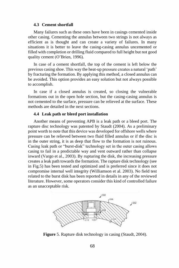
68
4.3 Cement shortfall
Many failures such as these ones have been in casings cemented inside
other casing. Cementing the annulus between two strings is not always as
efficient as is thought and can create a variety of failures. In many
situations it is better to leave the casing-casing annulus uncemented or
filled with completion or drilling fluid compared to full height but not good
quality cement (O’Brien, 1996).
In case of a cement shortfall, the top of the cement is left below the
previous casing shoe. This way the heat-up pressure creates a natural ‘path’
by fracturing the formation. By applying this method, a closed annulus can
be avoided. This option provides an easy solution but not always possible
to accomplish.
In case if a closed annulus is created, so closing the vulnerable
formations out in the open hole section, but the casing-casing annulus is
not cemented to the surface, pressure can be relieved at the surface. These
methods are detailed in the next sections.
4.4 Leak path or bleed port installation
Another means of preventing APB is a leak path or a bleed port. The
rapture disc technology was patented by Staudt (2004). As a preliminary
point worth to note that this device was developed for offshore wells where
pressure can be relieved between two fluid filled annulus or if the disc is
in the outer string, it is as deep that flow to the formation is not ruinous.
Casing leak path or “burst-disk” technology set in the outer casing allows
casing to fail in a predictable way and vent outward rather than collapse
inward (Vargo et al., 2003). By rupturing the disk, the increasing pressure
creates a leak path towards the formation. The rapture disk technology (see
in Fig.5) has been tested and optimized and is preferred since it does not
compromise internal well integrity (Williamson et al. 2003). No field test
related to the burst disk has been reported in details in any of the reviewed
literature. However, some operators consider this kind of controlled failure
as an unacceptable risk.
Figure 5. Rapture disk technology in casing (Staudt, 2004).
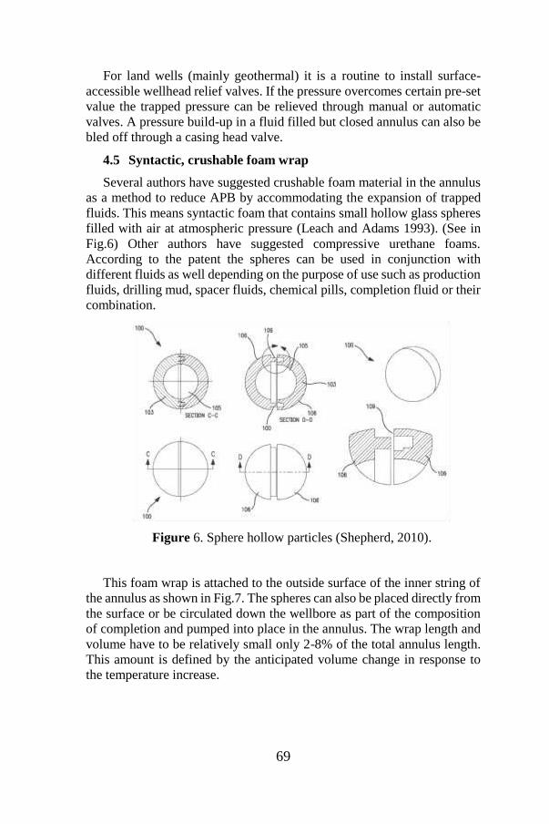
69
For land wells (mainly geothermal) it is a routine to install surface-
accessible wellhead relief valves. If the pressure overcomes certain pre-set
value the trapped pressure can be relieved through manual or automatic
valves. A pressure build-up in a fluid filled but closed annulus can also be
bled off through a casing head valve.
4.5 Syntactic, crushable foam wrap
Several authors have suggested crushable foam material in the annulus
as a method to reduce APB by accommodating the expansion of trapped
fluids. This means syntactic foam that contains small hollow glass spheres
filled with air at atmospheric pressure (Leach and Adams 1993). (See in
Fig.6) Other authors have suggested compressive urethane foams.
According to the patent the spheres can be used in conjunction with
different fluids as well depending on the purpose of use such as production
fluids, drilling mud, spacer fluids, chemical pills, completion fluid or their
combination.
Figure 6. Sphere hollow particles (Shepherd, 2010).
This foam wrap is attached to the outside surface of the inner string of
the annulus as shown in Fig.7. The spheres can also be placed directly from
the surface or be circulated down the wellbore as part of the composition
of completion and pumped into place in the annulus. The wrap length and
volume have to be relatively small only 2-8% of the total annulus length.
This amount is defined by the anticipated volume change in response to
the temperature increase.

70
Fig.7. Placement of sphere hollow particles around the string
(Leach and Adams, 1993).
The spheres are surrounded by placement fluid which is usually
followed by additional fluids (e.g. cement slurry) that usually do not mix
with the fluid around the particles. When annular pressure builds up the
spheres crush providing more space for the fluid to expand.
4.6 Compressible or shrinking fluid in the annulus
Two other methods can be found in the literature to mitigate APB. In
case of these two methods also fluid fills up the upper section of the annular
space above TOC.
4.6.1 Compressible fluid in the annulus
A method where compressible fluids are placed in the annulus to
balance the volume increase caused by thermal load is introduced in this
section. This method has already been successfully used for APB
mitigation in deepwater operations which are more inclined to this type of
failure (Vargo et al., 2003). This method has been tested and proved to be
effective in wells prone to annular pressure increase due to heat up.
Compressible fluid in the annulus means a nitrified foam spacer that is
placed above the top-of-cement in the annulus between two casing strings.
A reasonably small percentage of nitrogen, less than 5% of the trapped
volume, is adequate to form a compressible pad that can facilitate the
pressure increase. Pressure increase vs. increase in temperature with non-

71
foamed fluids and foamed fluids can be seen in Fig. 8 and Fig. 9,
respectively.
The theory of this method is shown in the Ideal Gas Law (Loder et al.,
2003). A decrease in the gas volume causes a small increase of pressure.
This relation is well described by Boyle’s Law that shows the pressure
change in a system is directly proportional to the change in volume (Eq.6).
𝑝1𝑉1 = 𝑝2𝑉2 (6)
Fig.8. Pressure increase
vs. increase in temperature
with non-foamed fluids
(Vargo et al. 2003).
Fig.9. Pressure
increase vs. increase in
temperature with foamed
fluids (Vargo et al. 2003)
Therefore, with this method the size of the pressure build-up can be
moderated from thousands to hundreds of kPa or psi above the placement
pressure. This magnitude is significant when the pressures become close
to the collapse pressure of a casing string.
4.6.2 Spacer fluid that shrinks
Annular fluids that shrink upon heating have been suggested as a means
to prevent APB. These may be pumped as a spacer before the cement
slurry which contains about 20-40% of emulsified methyl methacrylate
monomer (MMA). According to Bloys et al. (2008) MMA phase shrinks
by about 20% upon polymerization creating space for the other fluid’s
volume increase. Polymerization is initiated by heat, as seen in Fig.10 and
even the target temperature can be controlled and the earlier
polymerization can be blocked by appropriate type of initiator. The MMA
(10%-50% very sable emulsion) is emulsified into a simple water-based
fluid with densities from 0.96-1.8 g/cm3 that is planned to be the last spacer
before the cement.
This method has already been successfully tested in a 500 ft deep test
well in Bossier City, LA. In this test well a 7” casing was hanged inside of

72
9-5/8” casing. The bottom of the 7” casing was sealed with flapper valves
what allows the test fluids to be circulated through. The MMA
(concentration 28% of liquid phase) spacer was displaced into the annulus.
The annulus was sealed and heating started. Pressure increased but once
the target temperature was achieved polymerization and the quick pressure
drop begun.
Figure 10. Behaviour of water vs. a 14 ppg MMA emulsion
(Bloys et al., 2008).
4.7 VIT or VIC applications
Vacuum insulated tubing (VIT) has been successfully applied to
mitigate annular pressure build-up. VIT with thermal packer is an applied
insulation technique in case of steam injection procedures. However due
to difficulties vacuum insulated casing (VIC) as a completion technique
has been researched and used in some oilfield operation (Yue et al. 2013).
4.7.1 Vacuum insulated tubing (VIT) application
The vacuum insulated tubing is a piping system consists of an inner and
outer tubing welded together at both ends, as seen in Fig.11. The first
oilfield application happened in the Alaskan tundra to prevent flowline
subsidence. Since then, in many APB related cases VIT has been
recognized as a potential mitigation technique.
There are special areas where VIT has been applied successfully
(Azzola et al., 2004):
Enhanced oil recovery

73
SAGD
Prevention of paraffin build-up
Lessen the severity of cold start-up and hydrate formation
Temperature preservation for heavy oil flow through
Vacuum insulated tubing given its effective insulating capabilities can
prevent the annulus to be heated to the point when the fluid expansion
creates high enough pressure for casing or tubing damage. The piping sizes
ranges from 2” to 7” and usually the grade is L-80 or 13Cr. The circular
space between the two welded tubes is typically 0.15-0.5” wide. The space
contains aluminium wraps for reducing radiation, and a substance that
removes gas by sorption, also known as getter, in order to make the design
to be able to preserve the vacuum for about 10 years (Azzola et al., 2004).
Figure 11. Representation of a vacuum insulated tubing
(Ferreira et al., 2012).
An issue with VIT is that it is not able to provide a similar collapse and
burst resistance as a conventional tubing of the same size and grade.
According to (Yue et al. 2013), when a thermally loaded well is deeper
than 600 m VIT with thermal packer technique is recommended. Further
limitations of this technique is related to thermal packer`s mechanical
failure which sometimes so serious that it is not possible to continue steam
cycles. It also has workover problems if VIT is moved after steam injection
or economic problems if VIT is left in the well.

74
4.7.2 Vacuum insulated casing (VIC) application
In order to prevent problems and fulfill insulation, injection and
production expectations collectively vacuum insulated casing (VIC) can be
a viable technique.
It can be stated that VIC equals to VIT in manufacturing such as the
design theory, vacuum as insulation, materials, welding but VIC is also
different from VIT in function and its role in the well`s life (Yue et al.,
2013). VIC is an integral part of well completion, as seen in Fig.12.
Fig.12. VIC as part of
the well completion (Yue et al., 2013).
5. Summary APB resolutions
It can be concluded that there are numerous methods exist in the
literature for mitigating annular pressure build-up however only a small
percentage pay attention to the problem of trapped fluid in pockets or
channels. This special pressure buildup problem despite of all the applied
best practices cannot be eliminated; therefore prevention of fluid trapped
in pockets or channels behind the casing is the most important task.
Advantages of VIC compared to
VIT:
There is no packer
It avoids workover
It increases steam
flow area
While having their advantages
they inevitably have some
mechanical problems since the
welding technique is the same as in
case of VIT. This application is a new
technique and has only been tested
recently (Yue et al. 2013) however
VIC has great potential in different
thermal applications. As reported by
Yue et al. (2013) a field trial was
performed in several oilfileds in
China in more than 10 wells.

75
Table 1. Summary of the mitigation methods.
Mitigation
methods
Key
par
amet
ers
Mat
uri
ty
Use
in
th
erm
al
app
lica
tio
n
En
vir
on
men
tal
effe
ct
Tec
hn
olo
gy
avai
lab
ilit
y
Lo
gis
tics
Rel
ativ
e co
st
Reg
ula
tory
reco
mm
end
ed
pra
ctic
e
Sophisticated well design C comply
Full Height Cement C comply
Foamed Cement C comply
Resilient Cement D permit
Cement Shortfall C unallowe
d
Rapture Disk P N/A N/
A
unallowe
d
Relief Valve D permit
Crushable foam wrap P permit
Compressible fluid (N2) C permit
Shrinking fluid (MMA) P permit
VIT D comply
VIC P N/A N/A
C- commercial/often used
D- well developed/seldom
used
P- prototype/not used or only
tested
A table (Table 1) was prepared about a summary of the mitigation
methods that help in comparison and choose the best method for thermal
application.
6. Conclusions and recommendations
From the work conducted in this literature review, the following
conclusions are made:
Cement integrity have a key role in well integrity and if that have been
compromised casing collapse occurs caused by trapped annular liquid
behind the casing.
Steam injection means a great thermal load in a well. In case of trapped
fluid behind the casing pressure can access the collapse pressure when
76
fluid expands induced by 300°C injected steam. Trapped pressure
problem cannot be 100% eliminated therefore prevention its forming
is important.
There are numerous mitigation methods in the literature but not every
method can be applied for each drilled well. The final method depends
on regulatory board approval, logistics, reliability and cost.
A basic method in the industry is casing upgrading. In a thermal
application it is major to apply higher safety factors than in case of a
conventional application.
Applying full height good cement job is the best practice for wells
however the evaluation of the cement material can highly improve the
cement job in thermal wells. Testing foam cement, resilient cement or
cement with hollow microspheres may be conducted. Getting more
information on the behaviour of these materials is important as this
way reliable data can be served for further finite element analysis.
Also, a rarely examined parameter is cement permeability however it
is a main factor that reflects on the sealing capability of each cement
type. Important to note that the especially high temperature can also
create more changes in the cement material that expected therefore a
full testing can be necessary and useful. Testing of special material,
like hollow sphere cement at 300° can provide results that are novelty
for the industry since this type of testing has not been done before.
There are many potential methods for preventing trapped annular fluid
therefore testing of methods would be beneficial since this helps in
better understanding and more accurate planning for future
applications.
7. References
Azzola, J.H., Tselepidakis, D.P., Pattillo, P.D., Richey, J.F., Tinker, S.J., Miller,
R.A., Segreto, S.J. 2004. Application of Vacuum Insulated Tubing to Mitigate
Annular Pressure Buildup. SPE 90232, SPE Annual Technical Conference and
Exhibition, Houston, Texas, USA. 26-29 September 2004.
Bloys, B., Foley, R; Harvey, F; Davis, J; Cassel, T; Bloys, B; Gonzales, M;
Hermes, R; Daniel, J M. 2008. Trapped Annular Pressure Mitigation: A Spacer
Fluid That Shrinks: Update. IADC/SPE 112872, IADC/SPE Drilling
Conference, Orlando, Florida, USA. 4-6 March 2008
Bradley, H B. Petroleum engineering handbook. United States: N. p., 1987. Web.
Ferreira, M.V.D., Santos, A.R., Vanzan, V. 2012. Thermally Insulated Tubing
Application to Prevent Annular Pressure Buildup in Brazil Offshore Fields.

77
SPE 151044, SPE Deepwater Drilling and Completions Conference,
Galveston, Texas, USA. 20-21 June 2012.
Griffith, J.E., Lende, G., Ravi, K., Saasen, A., Nodland, N.E., Jordal, O.H. 2004.
Foam Cement Engineering and Implementation for Cement Sheath Integrity at
High Temperature and High Pressure. IADC/SPE 87194, IADC/SPE Drilling
Conference, Dallas, Texas, USA., 2-4 March 2004.
Hasan,A.R., Izgec, B., Kabir,C.S. 2009. Sustaining Production by Managing
Annular-Pressure Buildup. May 2010 SPE Production & Operations: 195-203,
SPE 120778,
Hole, H. 2008. Geothermal Well Design-Casing and Wellhead. Petroleum
Engineering Summer School, Dubrovnik, Croatia, Workshop #26 June 9-13,08
Kaldal, G.S., Jonssonm.P., Palsson, H., Karlsdottir, S.N. 2013. Collapse Analysis
of the Casing in High Temperature Geothermal Wells. Thirty-eight Workshop
on Geothermal Reservoir Engineering, Stanford, California, February 11-13,
2013
Kopp, K., Reed, S., Foreman,J., Carty, B., Griffith, J. 2000. Foamed Cement vs.
Conventional Cement for Zonal Isolation-Case Histories. SPE 62895, SPE
Annual Technical Conference and Exhibition, Dallas, Texas, October 1-4.
Leach, C.P., Adams, A.J. 1993. A New Method for the Relief of Annular Heat-Up
Pressures. SPE 25497, Production Operations Symposium, Oklahoma City,
Oklahoma, USA, March 21-23, 1993
Lepper, B.; Production Casing Performance In a Thermal Field; PETSOC-94-07.;
DOI: 10.2118/94-07
Loder, T., Evans, J.H., Griffith, J.E. 2003. Prediction of and Effective Preventative
Solution for Annular Fluid Pressure Buildup on Subsea Completed Wells-Case
Study. SPE 84270, SPE Annual Technical Conference and Exhibition, Denver,
Colorado, USA, 5-8 October 2003.
Matthews, C.; Tao, G.; Adams, A.; Special Considerations for Well Tubular
Design at Elevated Temperatures; SPE Drilling & Completion (2020); DOI:
10.2118/199570-PA
Moe, B., Erpelding, P. 2000. Annular Pressure Buildup: What it is and what to do
about it. Deepwater Technology, August 2000
O`Brien,T.B., Simpson,O.G. 1996. A Case Against Cementing Casing-Casing
Annuli. IADC/SPE 35106, IADC/SPE Drilling Conference, New Orleans,
Luisiana, USA, 12-15 March 1996.
Pattillo,P.D.,Cocales,B.W., Morey,S.C. 2004. Analysis of an Annular Pressure
Buildup Failure During Drill Ahead. SPE 89775, SPE Annual Technical
Conference and Exhibition, Houston, Texas
Rabia, H. Oilwell Drilling Engineering. Principles and Practice.
Graham&Trotman Ltd. London 1995. 322 p.1.

78
Southon, J.N.A. 2005. Geothermal Well Design, Construction and Failures.
Proceedings World Geothermal Congress 2005, Antalya, Turkey
Tahmourpour,F.,Hashki, K., Hassan, H. 2007. Different Methods to Avoid
Annular Pressure Buildup by Appropriate Engineered Sealant and Applying
Best Practices (Cementing and Drilling). SPE 110040, SPE Annual Technical
Conference and Exhibition, Anaheim, California
Tahmourpour,F.,Hashki, K., Hassan, H. 2007. Different Methods to Avoid
Annular Pressure Buildup by Appropriate Engineered Sealant and Applying
Best Practices (Cementing and Drilling). June 2010 SPE Drilling &
Completion: 248-254,
Thorhallsson, S. Geothermal well operation and maintenance. 2003 11.10.2017;
Available from: http://www.os.is/gogn/flytja/JHS-
Skjol/IGC2003ShortCourse/13Sverrir.pdf.
Barrier definitions and risk assessment tools for geothermal wells. Available from:
https://www.researchgate.net/publication/324573751_Barrier_definitions_an
d_risk_assessment_tools_for_geothermal_wells [accessed Apr 19 2021].
Yue, H., Pang, W., Zhang,T., He, Z., Hou, Q., Deng, D., Du, J., Mao, J., Zhao, X.,
Duan, Y. 2013. Integral Completion Technique for Heavy Oil Thermal
Recovery. SPE 165518, SPE Heavy Oil Conference Canada, Calgary, Alberta,
Canada
Vargo Jr., R.F., Payne, M., Faul, R., Leblanc, J., Griffith, J.E. 2003. Practical and
Successful Prevention of Annular Pressure Buildup on the Marlin Project. SPE
77473, SPE Annual Technical Conference and Exhibition, San Antonio,
Texas, USA, 29 September-2 October, 2002
Williamson, R., Sanders, W., Jakabosky, T., Serio, M., Griffith, J.E. 2003. Control
of Contained-Annulus Fluid Pressure Buildup. SPE/IADC 79875, SPE/IADC
Drilling Conference, Amsterdam, The Netherlands
Staudt, J. J. (2004). U.S. Patent No. 6,675,898. Washington, DC: U.S. Patent and
Trademark Office.
Shepherd, J.E,; Rakow, J.F.; Pattillo, Ii, P.D.; US Patent No. US2010/0113310
A1; 2010; Washington, DC: U.S. Patent and Trademark Office.

79
CHAPTER V
THE EVALUATION ON WATER STRUCTURE IN
MARDIN HISTORICAL MADRASAHS
F. Demet AYKAL
(Prof. Dr. ); Dicle University, Diyarbakır, Turkey,
e-mail: [email protected],
Orcid No: 0000-0003-2424-0407
Meltem ERBAŞ ÖZİL
(Asst. Prof. ) Dicle University, Diyarbakır, Turkey,
e-mail:[email protected],
Orcid No: 0000-0003-2077-8728
1. Introduction
Water has always been a basic and indispensable element for people.
The water, which has affected settlement and lifestyles of people
throughout history, is necessary for a healthy life. Water has the features
of rehabilitating, tranquillizing, relaxing and keeping people away from
stress in psychological respects. In addition to its vital importance, water
is an indispensable factor for landscape architecture. This factor welcomes
us as landscape elements, such as ornamental pool, water running on wall,
fountain in architectural respects.
The city of Mardin, located in the north of Mesopotamia, hosted people
from different religions and nationalities throughout history. These people
from different cultures lived together based on mutual respect. They have
built a cultural harmony in Mardin by still maintaining this way of life.
Respect has become a factor which is not only supporting people but also
buildings. The historical buildings in Mardin have survived until today by
challenging the destructive effects of time. Accordingly, it has made his
name known throughout the world as a cultural and historical city.
One of the group of buildings enabling the city to have a cultural and
historical characteristics is madrasahs. The abundance of historical
madrasahs in Mardin shows the importance given to education in the past
in the region. When examining madrasahs, which have generally similar
structural typologies, in detail, water features, bringing in sound and life to
these buildings, are seen. These water architecture features in madrasahs

80
were not only used for ornamental purposes but also used for its positive
effects on the psychology of user and representing cleaning and purity.
The aim of the paper was to analyze how art and techniques affected
water structure at the histo-rical madrasahs in the city Mardin and to
research about what functional contributions water made to madrasah
architecture except for using water as a landscape element.
2. Water Structure and Religional Relation
The structures, which must use water in order to function or built for
using water, are called water architecture structures (Tayla, 2007).
The water architecture has been used in order to build following
constructions from ancient periods: to collect snow and rainwater at
cisterns and reservoirs, and existing running water at weirs, especially in
Anatolia and to transfer this collected water to somewhere through
channels or tunnels with appropriate slopes, and to distribute water brought
to cities, to build pools, shadirvans and fountains in cities, to make
groundwater at low levels move to higher levels by containers, to drill
wells for using underground waters (Önge, 1997).
The first water systems in Turks were uncovered in Transoxiana. The
water needed by cities were brought by creating channels and waterways
on streams and rivers. Big water channels were used for agricultural areas.
In traditional civilizations, water is the symbol of purity, simplicity and
wisdom containing a mystical purification and cleaning power in itself. In
the Ottoman civilization, water became a factor bringing dynamic and
independent environment of nature to inner-city through public fountains,
water jets, pools, salsabil, cisterns, wells and etc. (Yüter, 2014)
Water was also regarded holy in polytheistic religions. In many cities,
there were senior judges appointed for caring fountains (Wycherley, 1993).
Hindus take bath in rivers during their religious rituals by believing to have
peace.
The water also has an important place in Judaism. It is directly related
to the creation of the world. Although it has not been recorded, we can
understand that the fountain next to the Wailing Wall in Jerusalem has a
religious meaning. It is significant that believers drink water from this
fountain before leaving after their worship at the Wailing Wall. It is
traditional for bathhouses in quarters, where Jewish people are in majority,
to have a big water basin and a private room is dedicated for this. The
Jewish people enter into this water basin after taking bath similar to full
ablution taken by Muslims. There are customs that water accumulations

81
(pools) are usually made where very important events occur. It is
commonly believed that pools have a curative function (Ertuğrul, 1989).
Water was considered to be holy in Christianity. Jesus said that “You
could not clean your heart by washing your body”. The water did not lose
its holiness during the period from the baptism of Jesus Christ to Ayazma,
and this holiness still goes on. Ayazmas are water resources believed to
provide cure, thus, regarded holy. It is also believed by people that
Ayazmas allow people to make their wishes come true, are cure for
diseases, enable anybody contacting them to redeem from his/her sins.
Water is an important element in Islam as it is in other religions. It is
stated in Islam’s holy book Koran that creation has begun with water and
every living creature has somewhat a relationship to water. “We have
created all living creature from water”. This civilization, enlivened with
water, has regarded water as a must for cleanliness next to faith and has
made water basis for its civilization (Sarı, 2016).
3. The General Characteristics of Mardin
The city of Mardin has been called by different names throughout
history. The city was named after by Assyrians as Merdin, Merdi, Merdo,
Mirdo, Merde, Marda, Mardin meaning castle or castles in Syriac
language; by Byzantines as Maride, Mardia; by Armenians as Merdin; by
Arabs as Maridin and by Ottomans as Mardin (Dolabani, 1972).
The establishment date of Mardin is not exactly known, it was
dominated by following civilizations from B.C. 3000 to today: Hurrians,
Akads, Babylonians, Hittites, Mitannies, Assyrians, Aramis, Meds,
Persians, Seleceons, Abgars, Romans, Abbasis, Hamdanis, Byzantines,
Sassanids, Marwanians, Turkmen, Seljuks, Artuks, Ayyubis, Mongolians,
Karakoyunlus, Akkoyunlus and Ottomans. Mardin was conquered by
Artuqids after 1071 Battle of Malazgirt and then conquered by the Ottoman
Empire in 1517 as a result of the Battle of Çaldıran (Cragoe, 2011).
Mardin lived its heyday in the period of Artuqids in architectural
respect. Today, most of the historical buildings in the city were built in this
period. Mardin madrasahs also belong to the period of Artuqids.
The city Mardin is one of the places whose sloping lands are used very
well. Its general view resembles huge stairs. Also, the streets with stairs or
ramps are often confronted due to its land structure. The depth of land
makes residential buildings cascaded. However, these steps are not in the
form of cubic elevators, but are integrated in a way that they are positioned
so as not to close each other's view (Demir, 2010) (Figure 1).
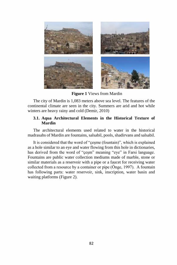
82
Figure 1 Views from Mardin
The city of Mardin is 1,083 meters above sea level. The features of the
continental climate are seen in the city. Summers are arid and hot while
winters are heavy rainy and cold (Demir, 2010)
3.1. Aqua Architectural Elements in the Historical Texture of
Mardin
The architectural elements used related to water in the historical
madrasahs of Mardin are fountains, salsabil, pools, shadirvans and salsabil.
It is considered that the word of “çeşme (fountain)”, which is explained
as a hole similar to an eye and water flowing from this hole in dictionaries,
has derived from the word of “çeşm” meaning “eye” in Farsi language.
Fountains are public water collection mediums made of marble, stone or
similar materials as a reservoir with a pipe or a faucet for receiving water
collected from a resource by a container or pipe (Önge, 1997). A fountain
has following parts: water reservoir, sink, inscription, water basin and
waiting platforms (Figure 2).

83
Figure 2 Historical Mardin Fountain
Salsabils are the most pleasant examples of the garden and water
architecture of palaces, waterside residences and mansions. Salsabils look
like an ornamented fountain at first glance. Water flows from a pipe at the
top in salsabils. The water pours into the bottom basin by flowing as small
waterfalls into the gradually made bowls on the front of the salsabil (Tayla,
2007) (Figure 3).
Figure 3 Historical Mardin Salsabil
Small fountains are little structures built at the outer court of a mosque
mostly at kulliyes. These structures have an appearance facing outward.
Their exterior surfaces are covered by metal bars reflecting the
characteristics of their periods. Small fountains are made up of one room,
and people are offered free water as charity. It is even known that sherbets
were offered in religious festivals and important days (Önge, 1997).
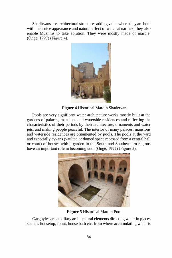
84
Shadirvans are architectural structures adding value where they are both
with their nice appearance and natural effect of water at narthex, they also
enable Muslims to take ablution. They were mostly made of marble.
(Önge, 1997) (Figure 4).
Figure 4 Historical Mardin Shadervan
Pools are very significant water architecture works mostly built at the
gardens of palaces, mansions and waterside residences and reflecting the
characteristics of their periods by their architecture, ornaments and water
jets, and making people peaceful. The interior of many palaces, mansions
and waterside residences are ornamented by pools. The pools at the yard
and especially eyvans (vaulted or domed space recessed from a central hall
or court) of houses with a garden in the South and Southeastern regions
have an important role in becoming cool (Önge, 1997) (Figure 5).
Figure 5 Historical Mardin Pool
Gargoyles are auxiliary architectural elements directing water in places
such as housetop, fount, house bath etc. from where accumulating water is

85
needed to be poured. Water finds its way with a chain. It is used for
accumulating water, especially in regions of insufficient rain (Figure 6).
Figure 6 Historical Mardin Gargoyle
3.2. Historical Madrasahs of Mardin and Their Water Elements
There are madrasahs in Mardin, which are still surviving since the 13th
century. There are seven (7) madrasahs registered at the Mardin provincial
directorate of culture and tourism as follows: Şehidiye Mosque and
Madrasah, Zinciriye Madrasah, Sıttı Radviyye (Hatuniye) Madrasah, Şah
Sultan Hatun Madrasah, Melik Mansur Madrasah, Altunboğa Madrasah,
Kasımiye Madrasah (Url-1, 2019).
The word “Medrese (Madrasah)” comes from the Arabic root of
“derase” and means “a place where it is studied and a building where
students live and study”. The madrasahs are buildings including rooms
dedicated to students studying and they have generally a yard at the middle
and rooms around this yard. Students may live and sleep here and attend
lessons in the mosque. There may be sometimes a shadervan at the middle
of yard of madrasahs, and there is mostly a portico in front of rooms
(Kansu, 1930).
The abundance of historical madrasahs in Mardin shows the importance
given to education in the past in the region. When it is examined in details
in madrasahs of which structural typologies are centred around the yard,
water elements, bringing in sound and life to the structure, are encountered.
The water elements in these madrasahs made of stone have an oasis feature
and take their place in the center of structure.
3.2.1. Şah Sultan Hatun Madrasah
This madrasah, consisting of ground + 1 floor, was built at the end of
the 15th century and the beginning of the 16th century. This structure with
a rectangle plan was built as an addenda to a mosque. Spaces arranged

86
around a yard with portico was built as two-storey. Today, you can see the
spaces in the north and the ruins of upstairs. The yard has a rectangle plan.
It is entered into space with a salsabil and two windows opening to the
yard through a door with a drop arch on which written basmala, at the north
of yard (Yıldız, 2008).
Its entrance is lancet arch and bonded with straight dimension stones.
The water of fountain flows towards the south. It is entered through stairs
to the fountain of which walls are made of ordered rubble stones. Water is
firstly poured to a circular trough and then to the second trough with a
rectangular plan (Figure 7-8).
Figure 7 Şah Sultan Hatun Madrasah Fountain and Trough
(Çağlayan, 2019)
Figure 8 Şah Sultan Madrasah and pool plan- section

87
3.2.2. Zinciriye Madrasah
It was built by Melik Necmeddin İsa Bin Davud in H. 787/AD.1385. It
has ground+1 floor. The building having a rectangular and wide-area
consists of a yard, mosque, tomb and student rooms. It is a two-storey
complex structure including spaces around a double yard (Yıldız, 2008).
Fountain and pool are at the center of yard. In addition, there is a
fountain connected to the street at the exterior facade of the mosque.
Fountains flow towards the south (Figure 9).
Figure 9 Fountain Plan-Section and Writing Arch at the Exterior
Façade of Zinciriye Madrasah (Çağlayan, 2019)
The fountain at the exterior façade of Zinciriye Madrasah provides
service for people on the street. The fountain was made of straight
dimension stones. Top cover of the fountain with an archway is cradle
vault. The plain façade is ornamented with stone network style. There are

88
ornamental writings at the end of arch along niche wall of fountain. This
fountain is out of use, which still survives.
The entrance of salsabil on the north of yard is lancet arch and its top is
covered by cradle vault. The salsabil is in a rectangular planned eyvan.
Salsabil, made of dimension stone material, has a plain façade. Black
stones on the façade and pool were added after restoration. Terraces at both
sides of the rectangular bath basin may also be used as a seat. (Figure 10).
Figure 10 Yard and Salsabils at Zinciriye Madrasah
The water of salsabil flows from pipe to bath basin and then to trough
and then the second trough and is finally accumulated in the pool at the
yard. The water flowing in four stages is in different rhythms and gives
sound to the place.
However, there is not a pool in the original plan of Zinciriye Madrasah.
Water had flown from a little pool at eyvan to a fountain in the street
located at the southern façade of the madrasah. The pool present at the yard
of Zinciriye was added during the restoration in 2007, thus, water flowing
to the fountain was cut (Soyukaya, Özgür, Kaya, 2013). It absorbs sounds
to come to a classroom from outside or other classrooms, therefore, it
enables students to concentrate on their lessons. It is claimed that the water
of fountain represents life while the water flowing from pipe represents
birth, the water from bath basin symbolizes childhood, the water from
trough represents youth, the waterway between trough and pool
symbolizes death, and pool represents heaven and eternal peace. The pool
at the center of the yard not only moisturize the air of madrasah but also
feed green plant around (Figure 11).

89
Figure 11 Plans and Appearances of Pool and Salsabil at Zinciriye
Madrasah
Gargoyle construction elements are generally responsible for throwing
rainwater out of the building. Yet, gargoyles at Zinciriye madrasah let
water come into the yard, and water is collected in the pool at the yard.
This water contributes to the refreshment of this place in Mardin where
there is little rain.
3.2.3. Kasimiye Madrasah
It was built between 1487 - 1502. It has a plan consisting of ordered
spaces around an open yard. It was built as a kulliye including a mosque,

90
tomb and madrasah. It has ground+1 floor on northern, eastern and western
facades while it has only one floor on southern facade (Yıldız, 2008).
The water of fountain in the north of Kasımiye madrasah flows towards
south. The top fountain with an entrance of lancet arch is covered by cradle
vault. The facade was enriched with straight dimension stone in different
colors. There is a fountain niche with a recessed stalactite. There are
ornaments on the lancet arch of fountain niche. The niche arch is placed on
a little pillar. There are two cup pockets on each side of the fountain niche
(Figure 12).
Figure 12 Kasimiye Madrasah Fountain
There is a pool at the center of madrasah. A story is told by local people
on eyvan and pool. It is told that the fountain, from which the water begins
to flow, symbolizes the birth, the beginning of life, this thick channel where
it poured first and the water flowed slowly, and seemed stationary,
represents the ages of babyhood, childhood and youth, the following thin
channel, in which water flows fast, symbolizes old age and the pool in
which water is collected represents the last judgment.
The water channel, beginning with the fountain at the middle of this
eyvan and then reaching the pool, results in an axis dividing the madrasah
into two from its yard.
It is believed that different points of pool symbolize ways to Heaven
and Hell, however, “all water will reach to Mesopotamian plain and every

91
creature dying with the thought that it gives life to a plant will somehow
find life in the plain.
It is known that pools were used in order to follow stars in the
Hellenistic period. (Wycherley, 1993) (Figure 13).
Figure 13 The Pool at the Center of Kasimiye Madrasah
The eyvan with salsabil seen commonly in Mardin architecture was
used not only for air conditioning and visual purposes but also for
educational purposes within the scope of astronomy lessons utilizing
reflections of stars on the pool (Mardin Metropolitan Municipality, 2017).
It is considered that there were pools at madrasahs, engaging in
education and science, for this purpose. Roof gargoyles of madrasahs were
designed so as to let water flow into the yard.
3.2.4. Altınboğa Madrasah (Tumbağa Tomb)
It was built in the middle of the 14th century in the Artuqids period. The
madrasah built by Altınboğa, the Vizier of Melik Mansur Ahmet Küçük,
is located at the end of dead-end street on the east of Zinciriye Madrasah
(Sultan İsa). The madrasah is devastated.
A deep eyvan, used as a fountain, and some other marks are only ruins
of the madrasah. The eyvan is in 2.80 x 4.70 m with a rectangular plan
enlarging from south to north and covered by cradle vault in the same
direction.
The eastern wall of eyvan was enriched by a lancet niche in 0.90 x 2.20
m. There is a door, opening to a water reservoir, in 1.15 m height and 0.90
m width and in rectangular form, on top of pipe. The work was made of
broken stone materials and is plain (Çağlayan, 2019).
After the entrance section remaining high, a deep room at the left
covered by cradle vault and reached by ascending a few stairs is seen. The
eyvan arch takes a step in front of this room and then arrived at the section
descended by two stairs.
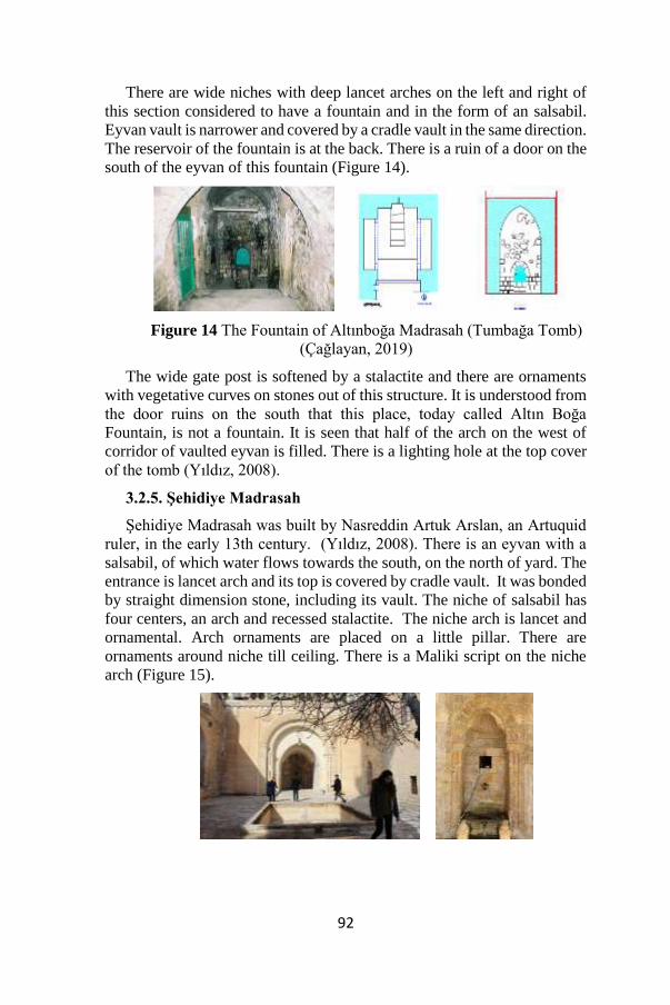
92
There are wide niches with deep lancet arches on the left and right of
this section considered to have a fountain and in the form of an salsabil.
Eyvan vault is narrower and covered by a cradle vault in the same direction.
The reservoir of the fountain is at the back. There is a ruin of a door on the
south of the eyvan of this fountain (Figure 14).
Figure 14 The Fountain of Altınboğa Madrasah (Tumbağa Tomb)
(Çağlayan, 2019)
The wide gate post is softened by a stalactite and there are ornaments
with vegetative curves on stones out of this structure. It is understood from
the door ruins on the south that this place, today called Altın Boğa
Fountain, is not a fountain. It is seen that half of the arch on the west of
corridor of vaulted eyvan is filled. There is a lighting hole at the top cover
of the tomb (Yıldız, 2008).
3.2.5. Şehidiye Madrasah
Şehidiye Madrasah was built by Nasreddin Artuk Arslan, an Artuquid
ruler, in the early 13th century. (Yıldız, 2008). There is an eyvan with a
salsabil, of which water flows towards the south, on the north of yard. The
entrance is lancet arch and its top is covered by cradle vault. It was bonded
by straight dimension stone, including its vault. The niche of salsabil has
four centers, an arch and recessed stalactite. The niche arch is lancet and
ornamental. Arch ornaments are placed on a little pillar. There are
ornaments around niche till ceiling. There is a Maliki script on the niche
arch (Figure 15).

93
Figure 15 The Salsabil Şehidiye Madrasah
There is an eight-strand star on the ground of bath basin. There is a
trough with sixteen-strand and star ornamented at the following section of
bath basin. (Figure 16).
Figure 16 Details of Bath Basin at Şehidiye Madrasah
The water flowing from pipe goes to bath basin and then trough and
finally the second trough. The difference in flow distances of water creates
different rhythms in water sound. The rhythmical water sound from
Salsabil functions as sound insulation (Figure 17).
Figure 17 Details of Trough at Şehidiye Madrasah

94
4. CONCLUSION
Human being needs water, which is vital for people, due to physical,
psychological and architectural purposes. As a result of these needs,
different techniques are applied to water in different fields so as to benefit
from it. In this study, the use of water in madrasahs were emphasized along
with its benefits in educational buildings.
Madrasahs are educational and scientific places. Madrasahs are mostly
considered to have the characteristics of religious structures. When
detailing these buildings, it is seen that they were designed for a functional
education. Since water-related elements generally flow towards south.
The madrasahs, built in the Artuqids period and still surviving, show
the importance given to education by Artuqids. It is not known whether the
reason for the absence of madrasahs belonging to the Ottoman period is
due to the fact that the existing madrasahs were considered sufficient or
because the Ottoman Empire did not attach the necessary importance to
education.
This research concludes that the water architecture was not only
performed for ornamental purposes but also educational, psychological and
physical needs. It is argued in this research carried out on the historical
madrasahs that water may also be used in the same purposes. The water
elements, which are not used sufficiently in today’s educational
institutions, can be used in this respect.
5. References
Cragoe C.D. (2011), How to Read Buildings? / Picture Building Reading
Guide, Yem Publishing, İstanbul.
Çağlayan M. (2019), An Architectural Comparison: Zinciriye and
Kasimiye Madrasahs in Mardin, Traces of History from the Early Ages
to the Modern Period II, Editors Prof. Dr. M. Doğan KARACOŞKUN
Prof. Dr. Osman Köse, Berikan Publishing, ISBN: 978-605-7501-36-3.
Demir M.M. (2010), Mardin City, İstanbul University, Social Sciences
Institute, İs-tanbul.
Demirağ D., Erten A., & Şen M. (2008), Culture coming with Water, İski,
transfer Yüter, F.Z. (2014), Water Architecture and Shadervan
Fountains in Istanbul, Haliç University, Institute Of Natural And
Applied Sciences.

95
Dolabani H. (1972), Mardin in History, Deyrulzafaran Monastery
Publications, pp: 195, İstanbul.
Ertuğrul Ö. (1989), The Aqua Architecture of the Byzantine Period in
Istanbul, Phd Thesis, İstanbul University, Social Science Institute,
İstanbul.
Kansu A.N. (1930), History of Education in Turkey, Muallim Ahmet Halit
Bookstore, İstanbul.
Mardin Travel Guide, (2017). Publication of Mardin Metropolitan
Municipality, Culture Tourism and Social Affairs Department,
November 2017.
Önge Y. (1997), Water Structures in Seljuk and Ottoman Periods in
Turkish Architecture, Turkish History Association, Ankara
Sarı İ. (2016), All Omans Water, Nokta Publishing, İstanbul.
Soyukaya N., Özgür M., Kaya F. (2013), Mardin Cultural Inventory,
Mardin Governorship & Çekül, İstanbul.
Tayla H. (2007), Building Systems and Elements in Traditional Turkish
Architecture, Taç Vakfı Publications, Vol:1 İstanbul.
URL-1. The Ministry of Culture and Tourism of the Republic of Turkey,
Mardin Provincial Culture and Tourism Directorate, Mosque - Madrasa
and islamic-ottoman social complexes,
http://www.mardinkulturturizm.gov.tr/TR,56509/camiimedrese-ve-
kulliyeler.html (E.T. 27 Aralık 2019).
Wycherley R.E. (1993), How Cities were Established in Ancient Times?
Archeology and Art Publications, İstanbul.
Yıldız İ. (2008), Aqua Architecture in Mardin, Yüzüncü Yıl University,
Social Science Institute, Van.
Yüter F.Z. (2014), Water architecture and shadervan fountains in Istanbul,
Master Thesis, Haliç University, Institute Of Natural And Applied
Sciences, İstanbul.

96
CHAPTER VI
SUSTAINABLE URBAN RENEWAL PROCESS AND
ASBESTOS FACTOR
Gülferah ÇORAPÇIOĞLU
(Asst. Prof. Dr.); Istanbul Arel University
e-mail: [email protected]
https://orcid.org/0000-0002-4748-3009
Sabit OYMAEL
(Prof. Dr) Istanbul Arel University
e-mail: [email protected]
https://orcid.org/0000-0003-2632-1139
1. Introduction
Asbestos is a natural mineral with a fibrous structure that is formed
when various silicate minerals are exposed to high pressure, temperature
and chemical impacts. It is medically proven to be cancerogenic, and its
use in especially the shipping, automotive and construction sectors due to
its impermeability and insulating properties constitutes such a serious
problem that it is in Group 1 of the list of Agency for Research on Cancer,
and is defined as carcinogenic (WHO, 2009). According to scientific
findings, the fibers have a low release probability, however when asbestos-
containing materials are subjected to repair, damage or disassembly, and
when weather conditions permit, the spread of asbestos fibers is possible.
When such fibers are released for any reason, the risk of the development
of diseases related to asbestos increases (Üzmezoğlu &Töreyin, 2017).
The first country to restrict the production and use of asbestos was Iceland
(1983), and the United Kingdom completely banned the use of asbestos in
1999 (Akboğa et al., 2017). Its use was banned in the EU member states
after ‘Regulation (EC) No 1907/2006 of the European Parliament of 18
December 2006 concerning the Registration, Evaluation, Authorisation
and Restriction of Chemicals’ came into effect (01.06.2007) (ECHA,
2006). In Turkey, with the revision in 2010 of the Regulation on the
Restrictions Relating to the Production, Supply to the Market and Use of
Certain Hazardous Materials, Products and Goods, published in the
Official Gazette (dated 26.12.2008, No. 27092), the launching, processing,
97
sale, import and production of all types of asbestos and asbestos products
were banned (Resmi Gazete, 2010), although banning asbestos does not
necessarily eliminate the problem. According to research, 500,000 tonnes
of asbestos were used in many products between 1983 and 2010 in Turkey,
and its deleterious effects still pose a threat when there is a need to
maintain, repair, disassemble, demolish and transport these products. As
exposure to this substance increases, so does the likelihood of developing
a disease (Topçu, 2002).
There are two types of asbestos minerals with the Mg3[Si2O5](OH)4
compound – serpentine and amphibole. Minerals from the serpentine group
are defined as chrysotile (white asbestos) CAS No12001-29-5, CAS
No132207-32-0, while minerals from the amphibole group are defined as
crocidolite (blue asbestos) CAS No12172-73-5, amosite (brown asbestos)
CAS No12172-73-5, actinolite (green asbestos) CAS No77536-66-4 and
tremolite (white-gray) CAS No77536-68-6 (Thompson, 1982). It has been
suggested that there are approximately 113 asbestos deposits in Turkey, 65
percent of which are chrysotile, 39 percent are tremolite and 1 percent are
crocidolite (Müller & Fischer, 2000). Asbestos fibers have been used in the
production of many cement composites due to their chemical structure and
their resistance to alkali environments (Ersoy, 2001). Chrysotile (white
asbestos) in particular has a binding characteristic and can absorb such
organic substances as resin and polymer (Akboğa et al., 2017). During our
research, chrysotile (white asbestos) was found in some concrete pipes in
Istanbul.
With the adoption of the Law on Converting of Areas Under Disaster
Risk dated and numbered 16.05.2012/6306 and its related regulation, the
urban renewal process began on 04.08.2012, and this led to the renewal of
old structures in areas where there is a high risk of earthquake. Urban
renewal projects, although aimed at creating healthy and livable cities,
come with adverse environmental problems on national and international
scales. The disassembly of construction components containing asbestos
comes with occupational and non-occupational environmental asbestos
problems. Based on the findings in literature regarding the delay in the
appearance of the consequences of asbestos exposure on human health, it
is apparent that the problem will prevail for years to come, despite the bans
and restrictions.
Contemporary studies aimed at decreasing and managing the adverse
effects of asbestos and other air pollutant wastes resulting from
disassembly and the recycling of hazardous waste have provided useful
perspectives on the matter. In one study it is stated that conducting an
environmental impact assessment (EIA) prior to embarking on the
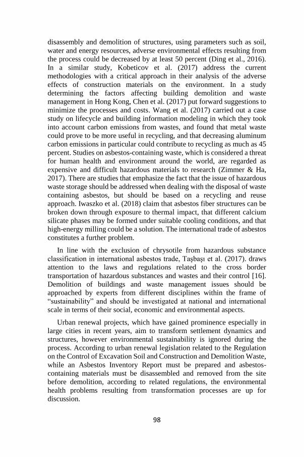
98
disassembly and demolition of structures, using parameters such as soil,
water and energy resources, adverse environmental effects resulting from
the process could be decreased by at least 50 percent (Ding et al., 2016).
In a similar study, Kobeticov et al. (2017) address the current
methodologies with a critical approach in their analysis of the adverse
effects of construction materials on the environment. In a study
determining the factors affecting building demolition and waste
management in Hong Kong, Chen et al. (2017) put forward suggestions to
minimize the processes and costs. Wang et al. (2017) carried out a case
study on lifecycle and building information modeling in which they took
into account carbon emissions from wastes, and found that metal waste
could prove to be more useful in recycling, and that decreasing aluminum
carbon emissions in particular could contribute to recycling as much as 45
percent. Studies on asbestos-containing waste, which is considered a threat
for human health and environment around the world, are regarded as
expensive and difficult hazardous materials to research (Zimmer & Ha,
2017). There are studies that emphasize the fact that the issue of hazardous
waste storage should be addressed when dealing with the disposal of waste
containing asbestos, but should be based on a recycling and reuse
approach. Iwaszko et al. (2018) claim that asbestos fiber structures can be
broken down through exposure to thermal impact, that different calcium
silicate phases may be formed under suitable cooling conditions, and that
high-energy milling could be a solution. The international trade of asbestos
constitutes a further problem.
In line with the exclusion of chrysotile from hazardous substance
classification in international asbestos trade, Taşbaşı et al. (2017). draws
attention to the laws and regulations related to the cross border
transportation of hazardous substances and wastes and their control [16].
Demolition of buildings and waste management issues should be
approached by experts from different disciplines within the frame of
“sustainability” and should be investigated at national and international
scale in terms of their social, economic and environmental aspects.
Urban renewal projects, which have gained prominence especially in
large cities in recent years, aim to transform settlement dynamics and
structures, however environmental sustainability is ignored during the
process. According to urban renewal legislation related to the Regulation
on the Control of Excavation Soil and Construction and Demolition Waste,
while an Asbestos Inventory Report must be prepared and asbestos-
containing materials must be disassembled and removed from the site
before demolition, according to related regulations, the environmental
health problems resulting from transformation processes are up for
discussion.

99
The purpose of this study is to conduct a research based on tangible data
regarding the existence, impact and severity of asbestos in building
demolitions within the scope of urban renewal in Turkey. To this end, an
experimental study is made of residential buildings in the process of
demolition in Istanbul-Kadikoy, where the prevalence of urban renewal
related demolitions and restorations has been increasing rapidly since
2012. In addition, observations are made regarding the compliance of the
demolition, disassembly and waste removal activities with current
regulations.
2. Material and Method
2.1. Examination of legislation
The study contains an analysis of the legislation and regulations related
to urban renewal, building demolition and waste that have been published
in the Official Gazette, including the “Regulation on Environmental
Impact Assessment” dated and numbered 25.11.2014/29186, and the
“Waste Management” regulation, dated and numbered 02.04.2015/ 29314
of the Ministry of Environment and Urban Planning. In addition, current
practices in the Kadikoy district of Istanbul have been evaluated in line
with the regulation on “Health and Safety Measures with respect to
Asbestos”, dated and numbered 25.01.2013/28539, and the regulation on
“Occupational Health and Safety in Construction Work”, dated and
numbered 05.10.2013/28786, of the Ministry of Labor and Social Security
(Resmi Gazete, 2014, 2015, 2013/01, 2013/10).
2.2. Experimental studies
In the experimental study conducted to detect whether the demolition
of buildings containing materials with asbestos content, samples from a
large number of construction materials were collected through a random
sampling method from three residential buildings located on Fahrettin
Kerim Gokay Street in the Zuhtu Pasa neighborhood of the Istanbul-
Kadikoy district, which was built prior to 1970 and is now undergoing
urban renewal. As seen in Appendix A, the number of samples was reduced
to 17, which were then sent to an accredited laboratory in plastic
packaging. The site and environmental conditions during the sampling
were not extraordinary, and sampling was carried out in accordance with
the regulation on “Health and Safety Measures with respect to Asbestos”
and “HSG 248-A2: Asbestos: The Analysts’ Guide for Sampling, Analysis
and Clearance Procedures”. A polarized light microscopy (Nikon/Eclipse,
200 MV POL) was used on all asbestos-type detection analyses for the
solid samples (agt. Vonka Lab). The results of the analysis were evaluated
taking into account the presence and type of asbestos minerals.
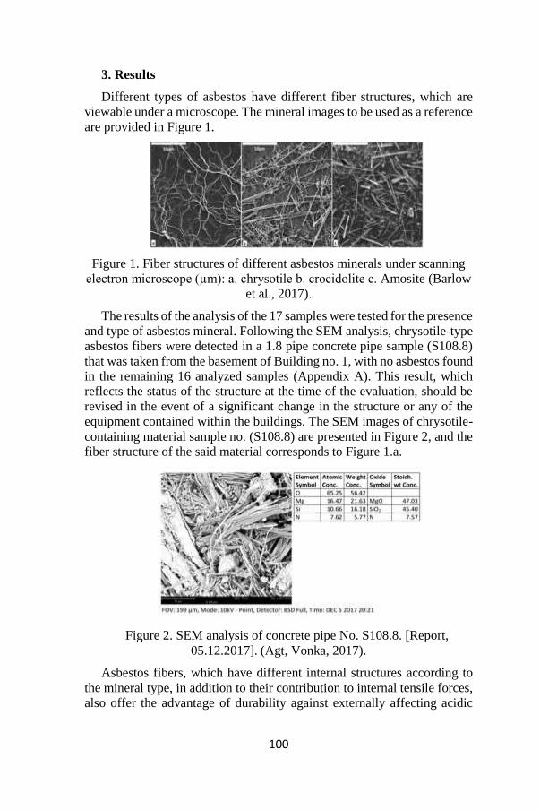
100
3. Results
Different types of asbestos have different fiber structures, which are
viewable under a microscope. The mineral images to be used as a reference
are provided in Figure 1.
Figure 1. Fiber structures of different asbestos minerals under scanning
electron microscope (µm): a. chrysotile b. crocidolite c. Amosite (Barlow
et al., 2017).
The results of the analysis of the 17 samples were tested for the presence
and type of asbestos mineral. Following the SEM analysis, chrysotile-type
asbestos fibers were detected in a 1.8 pipe concrete pipe sample (S108.8)
that was taken from the basement of Building no. 1, with no asbestos found
in the remaining 16 analyzed samples (Appendix A). This result, which
reflects the status of the structure at the time of the evaluation, should be
revised in the event of a significant change in the structure or any of the
equipment contained within the buildings. The SEM images of chrysotile-
containing material sample no. (S108.8) are presented in Figure 2, and the
fiber structure of the said material corresponds to Figure 1.a.
Figure 2. SEM analysis of concrete pipe No. S108.8. [Report,
05.12.2017]. (Agt, Vonka, 2017).
Asbestos fibers, which have different internal structures according to
the mineral type, in addition to their contribution to internal tensile forces,
also offer the advantage of durability against externally affecting acidic

101
and sulfate-based materials. The hazardous chemical materials in question
would have the highest impact on concrete pipes containing cement and
asbestos fibers. In the Kadikoy district, where all the analyzed and sampled
buildings are located, applications for urban renewal compliance
certificates are first directed to the Directorate of Environmental Protection
and Control, and experts from this directorate carry out site controls of the
building to be demolished and collect samples for analysis using statistical
methods. The collected samples are analyzed by laboratories with ISO/IEC
17025 accreditation and an asbestos inventory report is created. The report
includes data of the lab results, building description, analysis method,
location and approximate amounts of asbestos-containing materials. If no
asbestos is identified in the report, a certificate of compliance for urban
renewal is granted to the applicant company, and if asbestos is detected,
the materials must be removed using personal protective equipment in
accordance with the criteria in the Regulation on Health and Safety
Measures with respect to Asbestos. The resulting waste must be packaged
in accordance with the regulation and disposed of with a national waste
transportation form (Kadiköy Belediyesi, 2012). Asbestos is defined as
“asbestos-containing construction materials with code no. 17 06 05” on the
list of waste hierarchy in the Regulation on Hazardous Waste Control of
Ministry of Environment and Forestry, and is a class-1 hazardous waste
that requires systematic storage (Resmi Gazete, 2005).
4. Discussion and Conclusion
According to Kadikoy district regulations, asbestos-containing wastes
are disposed of at a class-1 systematic storage unit located in Sile
Komurcuoda, (İstaç, 2008) meaning that asbestos-containing materials are
expected to become harmless. An Asbestos Inventory Report is required to
be submitted in the event of building demolition in seven municipalities:
Kadikoy, Besiktas, Sisli, Maltepe, Atasehir, Tuzla and Bagcilar, out of the
39 municipalities in İstanbul. According to April 2017 data from the
Kadikoy Municipality, where the implementation is mandatory, 1,517
construction sites have been inspected since the asbestos inspection
process started in 2015, leading to the identification of asbestos-containing
materials in 446 buildings and the disposal of a total of 498.5 tonnes of
asbestos waste.
Looking at the results of the air quality measurements in Kadikoy, it is
observed that the values are much higher than international standards. The
World Health Organization (WHO) states that the 24-hour limit value for
(PM10) is 50 µg/m3 and 25 µg/m3 for (PM2.5); however, the values in
Kadikoy-Fikirtepe have been measured at 145.85 µg/m3 and 91.86 µg/m3,
respectively (Kadıköy Belediyesi, 2017) –much higher than the WHO

102
values – and should be considered as posing a serious threat to human
health. The danger to environmental health associated with asbestos
becomes clearer when it is considered as stated by Ersoy (2001), that
asbestos fibers with a diameter of as little as 0.01 µm. Üzmezoğlu and
Töreyin (2017) found out that when released into the air, can reach the
respiratory tract and accumulate in the lung tissue, and the risk of disease
increases proportional to the amount of asbestos fibers. Asbestos is highly
resistant to temperature, and its adverse environmental effects cannot be
eliminated, even by fire.
Based on the fact that approximately 90 demolition permits are granted
monthly in Kadikoy, and that five or six buildings may be being
demolished on a single city block at the same time, the management of
demolition and hazardous waste needs to be taken much more seriously.
There was no trace of asbestos, aside from the concrete pipe in the S108.8
sample, in the sample analysis carried out within the scope of this study.
As seen in Appendix A, no findings indicating the existence of persistent
organic pollutants – the use of which is banned and limited due to their
adverse effects on environmental and human health – aside from asbestos
were obtained. In line with these results, during the urban renewal process,
it is vital that more comprehensive studies are carried out, not only related
to asbestos, but also on the mitigation of other adverse environmental
impacts on air quality.
There are ongoing studies around the world into such topics as the
mitigation of the adverse environmental effects of building demolition,
waste sorting and recycling, minimizing demolition processes, planned
demolition, waste management and improvements to air quality. In
addition, it is observed that these studies are conducted with higher scale
designs in most countries. The air quality limit values set out in the
Regulation on Air Quality Assessment and Management by the Ministry
of Environment and Urbanization in Turkey are not compatible with those
of the European Union or the World Health Organization, and while these
values are expected to become compatible, it can be observed that the
action plans directed towards this purpose are not being executed and the
current laws are not being enforced due to a lack of inspections. In parallel
to the rapid urban renewal process, it is necessary to keep in mind that
environmental problems should be addressed with a serious approach, and
that this responsibility falls upon the respective ministries and local
administrations.
Opinions and objectives aimed at maintaining economic development
in the world in accordance with sustainable life limits are stated by
international organizations that deal with global environmental issues, such

103
as the United Nations Environment Programme (UNEP) and the European
Union (EU). It is emphasized that studies into this subject should be the
main concern of governments, planners, architects, preservationists and
groups of experts from different disciplines. It should further be kept in
mind that success can only be achieved if urban renewal is handled through
an integrated approach, and with the aim of preserving the entire set of
balances of a city. In this study, asbestos is examined within the context of
the urban renewal process and the environmental effects, and is discussed
within the framework of literature review data, experimental study results,
observations and related legislations. The study is expected to raise
awareness about the subject and to provide data for future studies. It would
be beneficial to take into consideration the following suggestions to ensure
a livable and sustainable environment:
• Creating awareness of living in a healthy environment across the
society, educating future generations on the subject, and conducting joint
activities between non-governmental organizations and public institutions,
• Taking control of the urban renewal process, ensuring compliance
with legislation and putting into force a more effective inspection
mechanism,
• Taking global standards related to demolitions and waste
management as an example, transforming recycling and disposal processes
into production from waste programs,
• Taking the asbestos factor into account in air quality
measurements, and focusing on the sources of pollution,
• Measuring concentrations of asbestos in the air that workers are
exposed to under the “Regulation on the Control of Excavation Soil and
Construction and Demolition Waste”, dated and numbered
18.03.2014/25406, and complying with the criteria that levels do not
exceed 0.1 fiber/cm³ in an 8 hour period,
• Health and environment experts to conduct joint studies to identify
the impact of demolitions as part of urban renewal projects on diseases
caused by asbestos,
• Conducting asbestos scanning of construction materials and
industrial material production sources, industrial buildings, and asbestos-
containing floors rather than buildings, and mapping asbestos sources.

104
References
Agt-Vonka. (2017). SEM Analizi Sonuçları, (Rapor- 05.12.2017). Agt,
Vonka Laboratuarı, İstanbul.
Akboğa-Kale, Ö., Gürcanlı, G. E., Baradan, S. (2017). Kentsel dönüşüm
sürecinde asbest maruziyeti ve alınması gereken önlemler. Pamukkale
Üniversitesi Mühendislik Bilimleri Dergisi, 23(6), 694-706.
Barlow, C. A., Sahmel, J., Paustenbach, D.J., Henshaw, J. L. (2017).
History of knowledge and evolution of occupational health and
regulatory aspects of asbestos exposure: 1900–1975. Journal of
Critical Reviews in Toxicology: 4, 286-316.
Chen, X., Lu, W. (2017). Identifying factors influencing demolition waste
generation in Hong Kong. Journal of Cleaner Production 141, 799-811.
Çevre ve Şehircilik Bakanlığı. (2008). Hava Kalitesi Değerlendirme ve
Yönetimi Yönetmeliği.
https://www.csb.gov.tr/db/cygm/editordosya/YON26898HavaKalitesi.
Ding, Z., Wang, Y., Zou, P.X.W. (2016). An agent based environmental
ımpact assessment of building demolition waste management:
conventional versus gren management. Journal of Cleaner Production
133, 1136-1153.
Ersoy, H.Y. (2001). Kompozit Malzemeler. Literatür Yayıncılık.
European Chemicals Agency. Reach Legislation. (2006).
https://echa.europa.eu/regulations/reach/legislation.
İstaç. Endüstriyel Atık Yönetimi. (2008). http://www.istac.istanbul.
İstanbul Asbest Raporu. (2018). TMMOB Çevre Mühendisleri Odası
İstanbul Şubesi.
https://www.tmmob.org.tr/sites/www.tmmob.org.tr/files/ikk_asbest_ra
poru_sayfalar_baski.pdf.
Kadıköy Belediyesi. Çevre Koruma ve Kontrol Müdürlüğü. (2012).
Binalarda Asbest Atıklarının Kontrolü.
http://www.kadikoy.bel.tr/Kurumsal/Mudurlukler/cevre-koruma-ve-
kontrol-mudurlugu.
Kadıköy Belediyesi. (2017). www.ebelediye.info/.../fikirtepe-deki-hava-
kalitesi-olcum-sonuclari.
Resmi Gazete. (2005). Tehlikeli Atıkların Kontrolü Yönetmeliği.
http://www.resmigazete.gov.tr/eskiler/2005/03/20050314-1.htm.

105
Resmi Gazete. (2010). Bazı Tehlikeli Maddelerin, Müstahzarların ve
Eşyaların Üretimine, Piyasaya Arzına ve Kullanımına İlişkin
Kısıtlamalar Hakkında Yönetmelik.
www.resmigazete.gov.tr/eskiler/2010/08/20100829-3.
Resmi Gazete. (2013). Asbestle Çalışmalarda Sağlık ve Güvenlik
Önlemleri Hakkında Yönetmelik.
www.resmigazete.gov.tr/eskiler/2013/01/20130125-24.htm.
Resmi Gazete. ( 2013). Yapı İşlerinde İş Sağlığı ve Güvenliği Hakkında
Yönetmelik. www.resmigazete.gov.tr/eskiler/2013/10/20131005.htm.
Resmi Gazete. (2014). Çevresel Etki Değerlendirmesi Yönetmeliği.
www.resmigazete.gov.tr/eskiler/2014/11/20141125.htm.
Resmi Gazete. (2015). Atık Yönetimi Yönetmeliği.
http://www.resmigazete.gov.tr/eskiler/2015/04/20150402-2.htm.
Iwaszko, J., Zawada, A., Lubas, M. (2018). Influence of high-energy
milling on structure and microstructure of asbestos-cement materials.
Journal of Molecular Structure, 1155, 51-57.
Kobeticov, K., Cerný, R. (2017). Ecotoxicology of building materials: a
critical review of recent studies. Journal of Cleaner Production, 165,
500-508.
Müller KM, Fischer M. (2000). Malignant pleural mesotheliomas: an
environmental health risk in Southeast Turkey. Journal of Thoracic
Medicine. 67(6), 608-609.
Taşbaşı, A., Sarıca, Y.P., Sabah, S. (2017). Uluslararası asbest ticareti. İş
Sağlığı ve Türkiye, Çalışma ve Toplum Dergisi, 4, 2003-2040.
Thompson, C.S., Levadie, B.(ed). (1982). Consequences of using ımproper
definitions for regulated minerals, definitions for asbestos and other
health-related silicates. ASTM Technical Publication.
Topçu, F. (2002). Asbest ve plevra. Solunum Dergisi (Eurasian Journal of
Pulmonology), 4 (Ek 1), 144-148.
Üzmezoğlu, B., Töreyin, N.Z. & Bayram, H. (Ed). (2017). Asbest nedir?
Asbestin sağlık üzerine etkisi. Türk Toraks Derneği Eğitim Kitapları.
Wang, J., Wu, H., Duan, H., Zillante, G., Zuo, J., Yuan, H. (2017).
Combining life cycle assessment and building ınformation modelling to
account for carbon emission of building demolition waste: a case study.
Journal of Cleaner Production, 1-13.
WHO (World Health Organization). (2009). International agency for
research on cancer, ıarc strengthens ıts findings on several carcinogenic

106
personal habits and household exposures, France.
https://www.iarc.fr/en/mediacentre/pr/2009/.../pr196_E.pdf.
Zimmer, A.T., Ha, H. (2017). People, planet and profit: unintended
consequences of legacy building materials. Journal of Environmental
Management, 204, 472-485.
Appendices
Appendix A. SEM (Scanning Electron Microscope) Analysis Table of
Samples.

107

108

109
CHAPTER VII
A COMPREHENSIVE OPTICAL LOSS ANALYSIS OF A
LINEAR FRESNEL REFLECTOR-PHOTOVOLTAIC
HYBRID SYSTEM WITH COMPUTER AIDED DESIGN
Keziban CALIK
Istanbul Technical University, Energy Institute, [email protected]
Orcid: 0000-0003-1348-3358
Coskun FIRAT
(Dr.); Istanbul Technical University, Energy Institute, [email protected]
Orcid: 0000-0002-2853-8940
1. Introduction
The optical efficiency of a linear Fresnel reflector (LFR) system which
can be defined as the ratio of the amount of solar radiation falling on the
receiver to the incoming solar radiation on the reflectors, is greatly
dependent on the system configuration. Besides the roughness of the mirror
surface, when an LFR system configuration made by considering the
parameters such as the mirror width (W), the distance between the mirrors
(S), the distance of each mirror to the tower (Q), the width of the receiver
(Wr), the height of the receiver (f) is not correct, then a serious decrease in
the overall system efficiency is observed due to optical losses. Optical
losses in LFR systems occur due to the mirrors shading and blocking each
other, the receiver shadow on the mirrors, the end losses and the edge
losses on the receiver. In systems with single axis solar tracking such as
LFRs, the cosine losses (transversal and longitudinal) are inevitable
because the incoming sun rays and the normal of the mirror surfaces might
not be in the same direction and because the mirrors don’t track the sun in
north-south direction as well.
To determine the optical efficiency in terms of the loss mechanisms
before constructing a linear Fresnel reflector system provides a very
important information on an optimum configuration. There are many
studies in the literature on determining the structure and the optical losses
in LFR systems. These studies are either done by using ray tracing software
or geometrical relationships between the optical parameters. The optical
losses are given inside the optical efficiency in most of the studies but not
as the amount of the lost itself. Therefore, to understand the optical losses
in details needs further researches.

110
The detailed expression on optical parameters for LFR systems is done
by Mathur et al. (1991a, 1991b). The LFR systems employing mirror
elements of both varying and equal width for three different absorber
configurations are analyzed in the study. In their study, the distribution of
the local concentration ratio on the surfaces of the absorbers has been
investigated using the ray trace technique. However, no any details about
the optical losses were given. Gouthamraj et al. (2013), have discussed the
design of a rooftop LFR solar concentrator module in terms of geometrical
parameters of the mirrors. However, there was no any detail about the
optical losses. In the study done by Gordon and Ries (1993), it was
proposed a new design concept for secondary concentrators that was
tailored to Fresnel reflector and analyzed the optical parameters however
there was no given detail on optical losses. Beltagy et al. (2017), have
presented a theoretical and experimental study of a prototype using Fresnel
type concentrator. In the study, the power received by the solar field was
calculated by considering the losses of cosine effect, shading of mirrors
and shading of the receiver. The results were verified experimentally
however, there was no detail about the losses. Zhu and Huang (2014) have
proposed a semi-parabolic linear Fresnel reflector solar concentrator. To
avoid the shading and blocking effects of the adjacent mirrors, it was
offered varying width mirrors located on a parabolic shaped base.
However, there was no any given detail for the losses. In the study done by
Hongn et al. (2015), end losses are analyzed analytically by using a simple
least square fitting and they give an expression to estimate the average
annual non-illuminated length and end loss. Chemisana et al. (2013) have
tried to design and test a method to assess the optical quality of solar
concentrators, based on the absorber reflection method. In the study, very
detailed information is given about the errors while the mirrors reflecting
the sun rays. Varying width of mirrors are offered to avoid the shading and
blocking loss, however no any details about the losses. Liu et al. (2014)
have investigated the relations between the structural parameters and the
optical performances of the system. In the study, the structural parameters
(W, S, Q) of the system are obtained and analyzed. However, instead of
giving details about optical parameters, it was focused on the concentrated
radiation distribution on the PV device (receiver) by making use of
software for tracing sun rays. Sallaberry et al. (2015) have focused on the
estimation of long-term optical losses due to the tracking error of a low-
temperature collector using low-concentration optics in their study. Balaji
et al. (2016) have studied on structural and optical parameters of an LFR
system in terms of secondary reflector in the receiver. Although the optical
efficiency was calculated, it was not supplied any details about the losses.
Tsekouras et al. (2018) have dealt with the optical and thermal
investigation of a linear Fresnel collector with trapezoidal cavity receiver.

111
The optical analysis is performed through the development of a ray-tracing
model in their study. Therefore, there was no any detailed information
about the losses individually. Bittencourt et al. (2015) have developed a
numerical model in order to obtain the optical efficiency of a solar collector
with a linear Fresnel concentrator. Their model is built based on the ray-
tracing and Monte Carlo methods.
In this study, optical losses in an LFR-PV hybrid system are analyzed
with the aid of computer by considering 9 realistic mirror-field
configurations. For each of the configuration, the loss because of the mirror
shadowing, mirror blocking, receiver shadowing, spillage and longitudinal
cosine effect (end loss) are calculated hourly for the representative days of
January, April, July and October as the seasonal representative months of
a year and presented as the annual average values. Later on, a relationship
is built in between the losses and the structure parameters of the LFR
system to get a fast understanding about the losses.
2. Precise determination of the optical losses
Besides the inevitable transversal and longitudinal cosine losses, the
optical losses in an LFR system (Fig.1) can occur due to the shadowing
and blocking of the adjacent mirrors, shadow of the receiver on the mirrors
and the edge losses due to the height of the receiver tower.
Figure 1 Demonstration of the optical losses in an LFR system.
When the incoming sun rays on a mirror is blocked by an adjacent
mirror then a shadow is occurred on the mirror which is called as
shadowing loss and when the sun rays reflected by a mirror is blocked by
an adjacent mirror then a blocking loss occurs as it is shown in the Fig.2
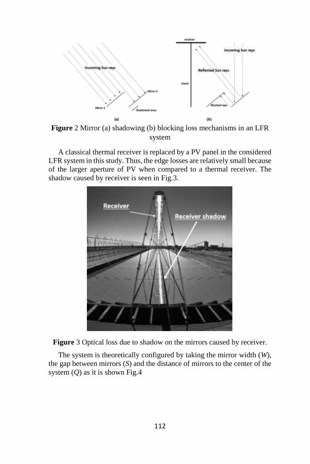
112
Figure 2 Mirror (a) shadowing (b) blocking loss mechanisms in an LFR
system
A classical thermal receiver is replaced by a PV panel in the considered
LFR system in this study. Thus, the edge losses are relatively small because
of the larger aperture of PV when compared to a thermal receiver. The
shadow caused by receiver is seen in Fig.3.
Figure 3 Optical loss due to shadow on the mirrors caused by receiver.
The system is theoretically configured by taking the mirror width (W),
the gap between mirrors (S) and the distance of mirrors to the center of the
system (Q) as it is shown Fig.4

113
Figure 4 Theoretical configuration of the LFR system
The LFR system is assumed to be located at 41.1051o N and 29.0225o
E (Ayazaga Campus of Istanbul Technical University, Turkey). The
monthly average hourly global solar radiation is calculated by using the
ASHRAE algorithm (Maleki et. al, 2017) for the optical calculations. The
months January, April, July and October are selected as the seasonal
representatives to make annual calculations. The radiation for every month
is averaged by taking the representative day of the month into account
(Anis et. al, 2019). To make the calculations, the sun is considered moving
on the transversal and the longitudinal plane of the system as showing in
the Fig.5
Figure 5 Geometrical parameters on the transversal plane of the system
(Çalık and Firat, 2019)

114
Nine different system configurations are considered as variations for
the optical losses. The length of the mirrors is taken as 3 m in all of the
variations. These variations are shown in Table 1.
Table 1 LFR System-configuration variations respect to mirror width
(W), Gap (S) and distance (Q)
VARIATIONS 1 2 3 4 5 6 7 8 9
Mirror width, W (mm) 300 300 300 400 400 400 500 500 500
Gap between mirrors, S, (mm) 100 200 300 100 200 300 100 200 300
Mirror to Center distance, Q, (mm) 400 500 600 500 600 700 600 700 800
Shadowed areas on each of the mirror are calculated with the help of
the computer aided graphics. The hours considered for the calculations are
selected according to the value of the radiation at that time of the day.
Therefore, the hours with low radiation levels are eliminated and this is
why the hours for the shadowing loss calculations are not matched with the
sunrise and sunset hours. For the given location, the solar radiation data for
the month January is given in the Table 2 as sample. The data for the other
months is obtained and calculated in the same way.
Table 2 Solar radiation data for January for the given location.
Local
time
Zenith angle
(degree)
Solar Azimuth
(degree)
Solar altitude
(degree)
Hourly DNI
(W/m2)
09.00 85.1 122.86 4.9 19.71
10.00 76.4 133.87 13.7 159.03
11.00 69.1 146.45 20.9 294.33
12.00 64.1 160.72 25.9 388.34
13.00 61.8 176.27 28.2 430.01
Solar noon 13.14 61.7 179.99 28.3 431.65
14.00 62.6 192.11 27.4 415.03
15.00 66.4 207.08 23.6 345.01
16.00 72.7 220.47 17.3 227.08
17.00 80.8 232.2 9.2 80.58
18.00 89.9 242.56 0.1 0.00
From Table 2, it can be seen that the considerable values of the average
hourly direct solar radiation (HDNI) are in between the hours 10:00 and
17:00 for the representative day of the January. Therefore, this interval of
hours is considered for the shadowing loss calculations. The average HDNI
for January is obtained as 292.43 W for the hours between 10:00 and 17:00.
Similarly, when the months April, July and October is considered as
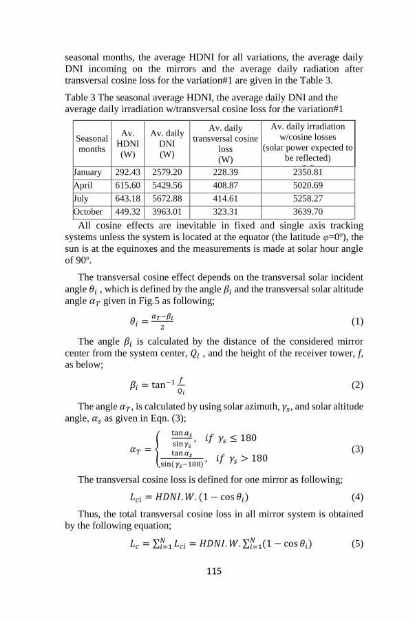
115
seasonal months, the average HDNI for all variations, the average daily
DNI incoming on the mirrors and the average daily radiation after
transversal cosine loss for the variation#1 are given in the Table 3.
Table 3 The seasonal average HDNI, the average daily DNI and the
average daily irradiation w/transversal cosine loss for the variation#1
Seasonal
months
Av.
HDNI
(W)
Av. daily
DNI
(W)
Av. daily
transversal cosine
loss
(W)
Av. daily irradiation
w/cosine losses
(solar power expected to
be reflected)
(W) January 292.43 2579.20 228.39 2350.81
April 615.60 5429.56 408.87 5020.69
July 643.18 5672.88 414.61 5258.27
October 449.32 3963.01 323.31 3639.70
All cosine effects are inevitable in fixed and single axis tracking
systems unless the system is located at the equator (the latitude φ=0o), the
sun is at the equinoxes and the measurements is made at solar hour angle
of 90o.
The transversal cosine effect depends on the transversal solar incident
angle 𝜃𝑖 , which is defined by the angle 𝛽𝑖 and the transversal solar altitude
angle 𝛼𝑇 given in Fig.5 as following;
𝜃𝑖 =𝛼𝑇−𝛽𝑖
2 (1)
The angle 𝛽𝑖 is calculated by the distance of the considered mirror
center from the system center, 𝑄𝑖 , and the height of the receiver tower, f,
as below;
𝛽𝑖 = tan−1 𝑓
𝑄𝑖 (2)
The angle 𝛼𝑇, is calculated by using solar azimuth, 𝛾𝑠, and solar altitude
angle, 𝛼𝑠 as given in Eqn. (3);
𝛼𝑇 = {
tan 𝛼𝑠
sin 𝛾𝑠, 𝑖𝑓 𝛾𝑠 ≤ 180
tan 𝛼𝑠
sin( 𝛾𝑠−180), 𝑖𝑓 𝛾𝑠 > 180
(3)
The transversal cosine loss is defined for one mirror as following;
𝐿𝑐𝑖 = 𝐻𝐷𝑁𝐼. 𝑊. (1 − cos 𝜃𝑖) (4)
Thus, the total transversal cosine loss in all mirror system is obtained
by the following equation;
𝐿𝑐 = ∑ 𝐿𝑐𝑖𝑁𝑖=1 = 𝐻𝐷𝑁𝐼. 𝑊. ∑ (1 − cos 𝜃𝑖)𝑁
𝑖=1 (5)
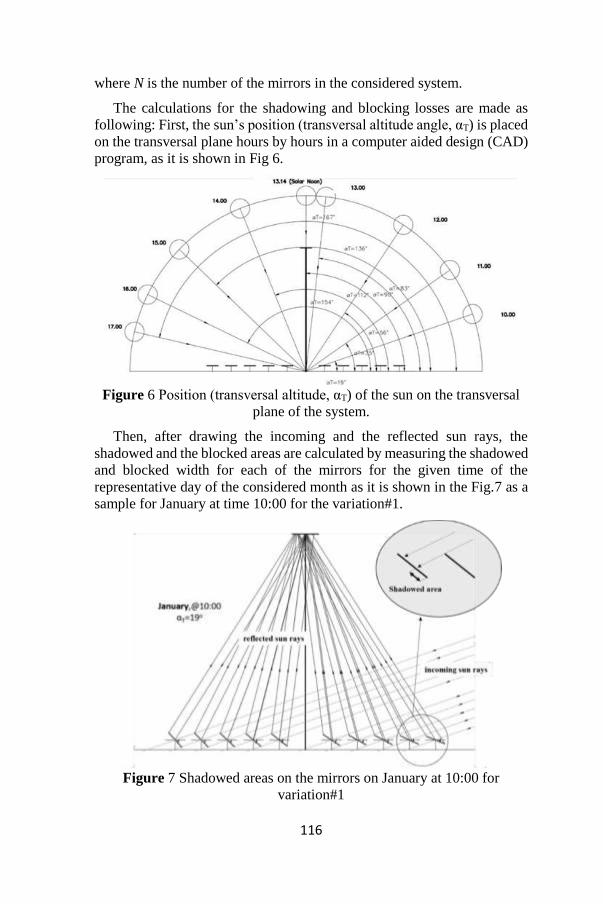
116
where N is the number of the mirrors in the considered system.
The calculations for the shadowing and blocking losses are made as
following: First, the sun’s position (transversal altitude angle, αT) is placed
on the transversal plane hours by hours in a computer aided design (CAD)
program, as it is shown in Fig 6.
Figure 6 Position (transversal altitude, αT) of the sun on the transversal
plane of the system.
Then, after drawing the incoming and the reflected sun rays, the
shadowed and the blocked areas are calculated by measuring the shadowed
and blocked width for each of the mirrors for the given time of the
representative day of the considered month as it is shown in the Fig.7 as a
sample for January at time 10:00 for the variation#1.
Figure 7 Shadowed areas on the mirrors on January at 10:00 for
variation#1

117
As an example, for the representative day of the month January (17th
Jan), there is seen no any blockage however the shadow by the mirror and
the amount of shadow on the 4th left mirror caused by an adjacent mirror is
measured as 104 mm as it is shown in the Fig.8.
Figure 8 The shadowing width for variation#1 on January at 10:00
Therefore, the shadowed area on 4th mirror is calculated as 0.31m2 for
the mirror length of 3m. Similarly, the measurements and the shadowed
and blocked area calculations are made for all of the mirrors for the given
system configuration and the results regarding shadowing area are given in
Table 4.
Table 4 Shadowed area values for each of the mirrors for the
representative day of the month January for variation#1
Local
time 10:00 11:00 12:00 13:00 14:00 15:00 16:00 17:00
Shading (m2) (m2) (m2) (m2) (m2) (m2) (m2) (m2)
Mirror
no
NO SHADING
1 0.38 0.09 0.00 0.00 0.20
2 0.37 0.066 0.021 0.30 0.56
3 0.34 0.033 0.033 0.32 0.58
4 0.31 0.00 0.042 0.33 0.59
5 0.00 0.00 0.048 0.34 0.59
Center
-1 0.00 0.00 0.00 0.25 0.53
-2 0.44 0.147 0.00 0.23 0.51
-3 0.44 0.159 0.00 0.20 0.49

118
-4 0.46 0.171 0.00 0.17 0.47
-5 0.47 0.18 0.00 0.00 0.00
As it is seen from Table 4, there is no any shadowing loss at some
certain hours and for some certain mirrors on the given day. The equivalent
shaded power on each of the mirrors on the representation day of January
for the variation#1 is presented in Table 5 by considering the hourly DNI
values given in Table 2.
Table 5 The lost power due to shadowing for January for variation#1
Local time 10.00 11.00 15.00 16.00 17.00
Mirror No Lost Solar Power due to Shading (W)
1 59.38 25.96 0.00 0.00 15.64
2 57.04 19.04 7.10 66.76 44.30
3 52.83 9.52 11.16 70.77 45.48
4 48.62 0.00 14.20 72.77 46.91
5 0.00 0.00 16.23 75.44 46.67
Center
-1 0.00 0.00 0.00 54.75 41.46
-2 67.79 42.40 0.00 50.07 40.04
-3 67.79 45.86 0.00 45.40 38.85
-4 71.07 49.32 0.00 37.39 37.19
-5 72.94 51.92 0.00 0.00 0.00
In the case of considering the shadowing loss, the total reflected net
solar power coming on the receiver will be obviously lesser than the solar
power expected to be reflected if there was no shadowing loss as it is given
in Table 6 for January for variation #1.
Table 6 Reflected net total solar power from mirrors after the shadowing
loss for the representative day of January for variation#1
Local time
Solar Power
expected to be
reflected
(W)
Power lost due to
mirror shading
(W)
The expected to be
reflected net power
after shadowing loss
(W)
10:00 1119.62 497.47 622.15
11:00 2259.12 244.02 2015.10
12:00 3217.50 - 3217.50
13:00 3720.79 - 3720.79
14:00 3531.20 - 3531.20
15:00 2750.91 48.69 2702.22

119
16:00 1666.18 473.35 1192.83
17:00 541.13 356.53 184.60
Average 2350.81 202.51 2148.30
The expected to be reflected solar power values given in Table 3 are
calculated as the product of the hourly DNI given in Table 2 and the
projective surface area of the tilted mirror (transversal cosine effect) whose
surface is covered with an aluminum lightning sheet with a very high
reflectance rate of 0.98 (ANOLUX, 2021). Similar calculations are
repeated for the representative days of April, July and October to obtain
the annual averaged values for the given LFR system variations as the
expected to be reflected power after mirror shadowing loss. As an example,
the monthly average-hourly solar radiation results for all of the months for
variation#1 are given in Table 7.
Table 7 The monthly average-hourly solar radiation values for
variation#1
Months Reflected power (with
cosine loss), (W)
Power loss due to
mirror shadowing, (W)
Net power to be
reflected, (W)
January 2350.81 202.51 2148.30 April 5020.69 280.07 4740.62 July 5258.27 289.26 4969.01 October 3639.70 248.02 3391.68 Average 4067.37 254.97 3812.40
It can be seen that the annual average-hourly shadowing loss in an LFR
system for the variation#1 is calculated as about 254.97 W. When the
measurements and the calculations are repeated for the other variations, the
results obtained for annual average shadowing loss, expected-reflected
power, net reflected power after shadowing loss and the total area of the
LFR system for given configuration are presented in the Table 8.
Table 8 System and the yearly average hourly solar radiation values for
all variations
Var.s Width
(mm)
Gap
(mm)
Dist.
(mm)
Mirrors
area
(m2)
System
Area
(m2)
Power with
transversal
cosine loss
(W)
Shadowing
loss
(W)
Reflected
Power after
shadowing loss
(W)
1 300 100 400 9 12.9 4067.37 254.97 3812.40
2 300 200 500 9 15.9 3749.17 116.00 3633.17
3 300 300 600 9 18.9 4001.23 59.73 3941.5
4 400 100 500 12 16.2 5380.33 417.94 4962.39
5 400 200 600 12 19.2 5334.97 217.84 5117.13
6 400 300 700 12 22.2 5288.79 127.52 5161.27
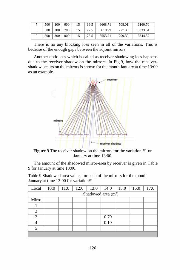
120
7 500 100 600 15 19.5 6668.71 508.01 6160.70
8 500 200 700 15 22.5 6610.99 277.35 6333.64
9 500 300 800 15 25.5 6553.71 209.39 6344.32
There is no any blocking loss seen in all of the variations. This is
because of the enough gaps between the adjoint mirrors.
Another optic loss which is called as receiver shadowing loss happens
due to the receiver shadow on the mirrors. In Fig.9, how the receiver-
shadow occurs on the mirrors is shown for the month January at time 13:00
as an example.
Figure 9 The receiver shadow on the mirrors for the variation #1 on
January at time 13:00.
The amount of the shadowed mirror-area by receiver is given in Table
9 for January at time 13:00.
Table 9 Shadowed area values for each of the mirrors for the month
January at time 13:00 for variation#1
Local
time
10:0
0
11:0
0
12:0
0
13:0
0
14:0
0
15:0
0
16:0
0
17:0
0 Shadowed area (m2)
Mirro
r no
1
2
3 0.79
8
4 0.10
5
5

121
-1 0.90
0
-2
-3
-4
-5 0.71
7
The amount of the loss in terms of power is shown in Table 10.
Table 10 The lost power due to receiver shadowing for January at time
13:00 for variation#1
Local time 12:00 13.00 14.00
Mirror No Lost Power due to Receiver-Shading (W)
1
2
3 324.57
4 42.71
5
Center
-1 379.27
-2
-3
-4
-5 272.87
Total 272.87 379.27 367.28
The longitudinal cosine loss (or the end loss) causes some receiver area
as not illuminated and it is calculated by the longitudinal solar incident
angle which is given with the following equation,
𝜃𝐿 = 𝐴𝑟𝑐𝑡𝑎𝑛(cos 𝛾𝑠 tan 𝜃) (6)
where 𝜃 is the solar incident angle which is defined as below;
cos 𝜃 = sin 𝛿 sin 𝜑 + cos 𝛿 cos 𝜑 cos 𝜔 (7)
𝜑 is the latitude of the system location and the solar declination angle and
the solar hour angle are defined as the following respectively,
𝛿 = 23.45 sin [360
365(𝑑 + 284)] (8)
𝜔 = 15𝑜(𝑡 − 12) (9)

122
d is the day number of the year and t is the local solar hour. The longitudinal
cosine loss is calculated by the Eqn. (10) and the effect is sketched up in
the Fig. 10.
𝐿𝑐𝐿 = 𝐻𝐷𝑁𝐼. 𝐿. 𝑊. (1 − cos 𝜃𝐿)(1 − cos 𝜃𝑖) (10)
Figure 10 The sketch of the longitudinal cosine effect.
It is clear that through the equations (1) to (10), the transversal and the
longitudinal cosine losses include all information about the sun’s position
in the sky, the solar radiation in the location and the mirror’s geometry
regarding to the sun’s position.
As an example, the hourly end loss (longitudinal cosine loss) for the
representative day of January (d=17) for the variation#1 is presented in the
Table 11.
Table 11 The hourly end loss for the representative day of January
(d=17) for the variation#1
Local
time 𝜔
(deg.)
𝛿
(deg.)
𝛾𝑠
(deg.)
𝜃𝐿
(deg.)
Lost
area
(m2)
HDNI
(W)
Long.
cosine
loss (W)
10:00 131.49 -20.68 133.87 35.32 0.15 159.03 23.71
11:00 146.49 -20.67 146.45 30.20 0.11 294.33 32.35
12:00 161.49 -20.67 160.72 24.49 0.07 388.34 28.30
13:00 176.49 -20.66 176.27 20.62 0.05 430.01 22.32
14:00 191.49 -20.65 192.11 22.20 0.06 415.03 24.93
15:00 206.49 -20.64 207.08 27.55 0.09 345.01 31.68

123
16:00 221.49 -20.63 220.47 33.06 0.13 227.08 29.77
17:00 236.49 -20.62 232.20 37.73 0.17 80.58 13.65
Table 11 shows that the average hourly longitudinal cosine loss (end
loss) in January for the variation#1 is just 25.84 W.
Some of the reflected sun rays towards the receiver is not collected by
the receiver and they escape back in to the space (ray-spillage), this causes
an optical loss which is called as edge loss. No edge losses are observed in
variation#1. However, this loss is observed in other variations and is
included in the calculations. In Fig. 11, the edge loss is shown for January
at time 12:00 for the variation#8 as an example.
Figure 11 The end losses for the variation #8 on January at time 12:00.
The amount of the edge loss for the variation#8 is given in Table 12 in
terms of the lost area and the lost solar power for January for the hours
10:00 to 17:00. The lost power is calculated by multiplying the reflected
solar irradiation (W/m2) and the lost area related to ray-spillage.
Table 12 The amount of the edge loss for the representative day of
January for variation#8
Local
time
The length of lost
area (m)
Lost edge area,
(m2)
Power lost due to spillage,
(W) 10:00 0.182 0.55 85.09
11:00 0.226 0.68 195.56
12:00 0.344 1.03 392.75

124
13:00 0.318 0.95 402.03
14:00 0.339 1.02 413.64
15:00 0.344 1.03 348.93
16:00 0.197 0.59 131.52
17:00 0.170 0.51 40.27
All of the optical losses occur on the representative day of July for the
variation#8 is given in Table 13 as an example.
Table 13 The optical losses occur on the representative day of July for the
variation#8
Local
time
Power
with
transversal
cos. loss
(W)
Mirror
shading
loss
(W)
Receiver
shading
loss
(W)
Edge
loss
(W)
End
loss
(W)
Net
power on
the
receiver
(W)
07:00 1418.15 602.23 58.40 60.09 697.42
08:00 3916.92 830.29 184.07 238.12 2664.43
09:00 6682.08 350.28 9.37 6322.44
10:00 9370.21 556.74 242.44 8571.03
11:00 11674.54 692.90 867.38 434.16 9680.09
12:00 13294.03 594.77 925.82 635.59 11137.84
13:00 13988.57 890.48 768.06 12330.03
14:00 13639.41 1119.26 933.19 696.89 10890.07
15:00 12305.30 699.15 751.91 503.55 10350.70
16:00 10199.49 692.64 783.18 309.63 8414.03
17:00 7602.45 416.51 104.65 7081.29
18:00 4825.47 827.67 235.30 405.46 3357.04
19:00 2189.78 937.31 96.65 98.60 1057.22
Direct normal irradiation (DNI), incoming power including transversal
cosine loss (𝑃𝑐), average annual (as the average of the seasonal
representative months of January, April, July and October) optical losses
(the transversal cosine loss, 𝐿𝑐, the mirror shadowing loss, 𝐿𝑚, the receiver
shadowing loss, 𝐿𝑟, the edge loss, 𝐿𝑒, and the longitudinal cosine loss (end
loss), 𝐿𝑐𝐿) and the total optical efficiency, 𝜂𝑜𝑝 , calculated according to
Eq.11 are given in Table 14 for all variations.

125
The total optical efficiency can be calculated as following;
𝜂𝑜𝑝 = 1 −𝐿𝑚+𝐿𝑟+𝐿𝑒+𝐿𝑐𝐿
𝑃𝑐 (11)
Table 14 Average annual optical losses and total optical efficiency of the
system
Variations DNI 𝑃𝑐, (W) 𝐿𝑐,
(W)
𝐿𝑚,
(W)
𝐿𝑟,
(W)
𝐿𝑒 ,
(W)
𝐿𝑐𝐿,
(W)
𝜂𝑜𝑝,
(%)
1 4411.25 4067.36 344 254.97 198 0 92.92 86.58
2 4411.25 4035.25 376 116.00 182 0 101.65 90.10
3 4411.25 4001.23 410 59.73 130 0 109.75 92.52
4 5881.55 5380.33 501 417.94 228 115 134.92 83.34
5 5881.55 5334.97 547 217.84 177 181 147.07 86.45
6 5881.55 5288.79 593 127.52 145 249 159.22 87.12
7 7351.94 6668.71 683 508.01 236 344 183.99 80.93
8 7351.94 6610.99 741 277.35 209 433 200.19 83.06
9 7351.94 6553.71 798 209.39 227 532 216.15 81.93
Hence, it can be built a relationship between the mirror shadowing loss
(𝐿𝑚), the receiver shadowing loss (𝐿𝑟), the edge loss (𝐿𝑒), optical
efficiency (𝜂𝑜𝑝) and the structure parameters width (W) and gap (S) as well
as transversal (𝐿𝑐) and longitudinal cosine losses (𝐿𝑐𝐿) by using a multiple
regression (MR) analysis (Darlington and Hayes, 2017). This relation
might satisfy very useful information about the optical losses and the
structure parameters before constructing an LFR system. Hence, by using
an MR, these relations are obtained as follows respectively:
𝐿𝑚 = −212.89 + 32.26𝑊 − 7.54𝑆 + 3.01𝐿𝑐 − 15.74𝐿𝑐𝐿 (12)
𝐿𝑟 = −39.08 + 16.77𝑊 + 1.39𝑆 − 13.04𝐿𝑐 + 45.24𝐿𝑐𝐿 (13)
𝐿𝑒 = 353.26 − 56.49𝑊 − 14.40𝑆 + 8.60𝐿𝑐 − 15.87𝐿𝑐𝐿 (14)
𝜂𝑜𝑝 = 76.52 + 1.09𝑊 + 0.55𝑆 − 0.20𝐿𝑐 + 0.42𝐿𝑐𝐿 (15)
As an example, the shadowing loss presented in Table 14 and the values
obtained by Eq. (12) are given in the Fig.12. It can be seen a good match
between the values. Therefore, one can calculate all of the optical losses
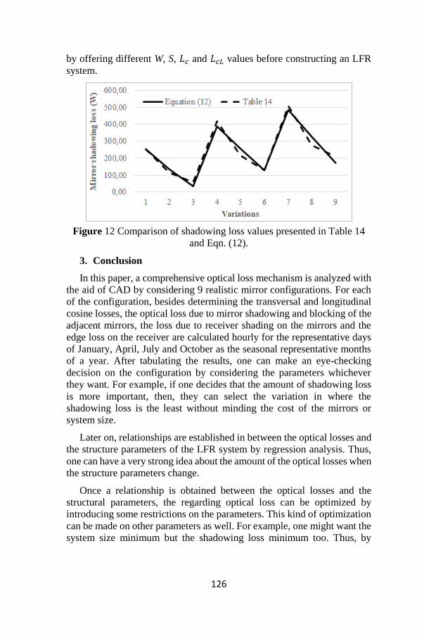
126
by offering different W, S, 𝐿𝑐 and 𝐿𝑐𝐿 values before constructing an LFR
system.
Figure 12 Comparison of shadowing loss values presented in Table 14
and Eqn. (12).
3. Conclusion
In this paper, a comprehensive optical loss mechanism is analyzed with
the aid of CAD by considering 9 realistic mirror configurations. For each
of the configuration, besides determining the transversal and longitudinal
cosine losses, the optical loss due to mirror shadowing and blocking of the
adjacent mirrors, the loss due to receiver shading on the mirrors and the
edge loss on the receiver are calculated hourly for the representative days
of January, April, July and October as the seasonal representative months
of a year. After tabulating the results, one can make an eye-checking
decision on the configuration by considering the parameters whichever
they want. For example, if one decides that the amount of shadowing loss
is more important, then, they can select the variation in where the
shadowing loss is the least without minding the cost of the mirrors or
system size.
Later on, relationships are established in between the optical losses and
the structure parameters of the LFR system by regression analysis. Thus,
one can have a very strong idea about the amount of the optical losses when
the structure parameters change.
Once a relationship is obtained between the optical losses and the
structural parameters, the regarding optical loss can be optimized by
introducing some restrictions on the parameters. This kind of optimization
can be made on other parameters as well. For example, one might want the
system size minimum but the shadowing loss minimum too. Thus, by

127
introducing a restriction on shadowing loss, the system size might be
maximized.
References
Anis MD.S., Jamil B., Ansari MD.A., Bellos E. (2019). “Generalized
models for estimation of global solar radiation based on sunshine
duration and detailed comparison with the existing: A case study for
India”, Sust. Energy Tech. and Asses., 31, 179–198.
ANOLUX Miro Silver, http://anomet.com/reflective-aluminum, (accessed
01/04/2021).
Balaji S., Reddy K.S., Sundararajan T. (2016). “Optical modelling and
performance analysis of a solar LFR receiver system with parabolic and
involute secondary reflectors”, Applied Energy, 179, 1138–1151.
Beltagy H., Semmar D., Lehaut C., Said N. (2017). “Theoretical and
experimental performance analysis of a Fresnel type solar
concentrator”, Ren. Energy, 101, 782-793.
Bittencourt A., Pigozzo V.C., Passos J.C., Cascaes G.M., Burigo A.
(2015). “Geometrical Parametric Analysis to Find Optimum
Configuration of a Solar Concentrator Workbench Using Linear Fresnel
Technology”, ISES Solar World Congress, Daegu, Korea, 08-12
November 2015, DOI:10.18086/swc.2015.10.06.
Calik K., Firat C., (2019). “A Cost-Effective Theoretical Novel
Configuration of Concentrated Photovoltaic System with Linear
Fresnel Reflectors”, J. of Polytechnic, 22:3, 583-589.
Chemisana D., Barrau J., Rosell J.I., Abdel-Mesih B., Souliotis M., Badia
F. (2013). “Optical performance of solar reflective concentrators: A
simple method for optical assessment”, Renewable Energy, 57, 120-
129.
Darlington R.B., Hayes A.F., (2017). Regression Analysis and Linear
Models: Concepts, Applications, and Implementation, The Guilford
Press, New York, USA.
Gordon J. M., Ries H. (1993). “Tailored edge-ray concentrators as ideal
second stages for Fresnel reflectors”, Applied Optics, 32:13, 2243-
2251.

128
Gouthamraj K., Jamuna Rani K., Satyanarayana G. (2013). “Design and
Analysis of Rooftop Linear Fresnel Reflector Solar Concentrator”, Int.
J. of Eng. and Innovative Tech., 2:11, 2013, 66-69.
Hongn M., Flores Larsen S., Gea M., Altamirano M. (2015). “Least square
based method for the estimation of the optical end loss of linear Fresnel
concentrators”, Solar Energy, 111, 264–276.
Liu Y., Hu P., Zhang Q., Chen Z. (2014). “Thermodynamic and optical
analysis for a CPV/T hybrid system with beam splitter and fully tracked
linear Fresnel reflector concentrator utilizing sloped panels”, Solar
Energy, 103, 191– 199.
Maleki S.A.M., Hizam H., Gomes C. (2017). “Estimation of Hourly, Daily
and Monthly Global Solar Radiation on Inclined Surfaces: Models
Revisited”, Energies, 10, 134.
Mathur S.S., Kandpal T.C., Negi B. S. (1991a). “Optical design and
concentration characteristics of linear Fresnel reflector solar
concentrators-I. Mirror elements of varying width”, Energy Conversion
and Management, 31:3, 205-219.
Mathur S.S., Kandpal T.C., Negi B. S. (1991b). “Optical design and
concentration characteristics of linear Fresnel reflector solar
concentrators-II. Mirror elements of equal width”, Energy Conversion
and Management, 31:3, 221-232.
Sallaberry F., García De Jalón A., Torres J., Pujol-Nadal R. (2015).
“Optical losses due to tracking error estimation for a low concentrating
solar collector”, Energy Conv. and Management, 92, 194–206.
Tsekouras P., Tzivanidis C., Antonopoulos K. (2018). “Optical and
thermal investigation of a linear Fresnel collector with trapezoidal
cavity receiver”, App. Thermal Eng., 135, 379–388.
Zhu J., Huang H. (2014). “Design and thermal performances of Semi-
Parabolic Linear Fresnel Reflector solar concentration collector”,
Energy Conv. and Management, 77, 733–737.

129
CHAPTER VIII
AROMATIC COMPOUNDS OF PROTEOLYSIS AND
LIPOLYSIS ORIGIN OCCURRING DURING
FERMENTATION IN MEAT PRODUCTS
Özgür KARADAŞ
(PhD Student ); Tekirdağ Namık Kemal University, Tekirdağ, Turkey
e-mail: [email protected], Orcid ID: 0000-0002-7379-7845
Binnur KAPTAN
(Asst. Prof. Dr. ); Tekirdağ Namık Kemal University, Tekirdağ, Turkey
e-mail: [email protected], Orcid ID: 0000-0002-6268-7245
İsmail YILMAZ
(Prof. Dr. ); Tekirdağ Namık Kemal University, Tekirdağ, Turkey
e-mail: [email protected], Orcid ID: 0000-0003-1116-0934
1. Introduction
Meat, which has been important in terms of our diet from the ancient
times till present day, is the source of minerals, vitamins, proteins and
different bioactive compounds (conjugated linoleic acid, peptides, taurine,
creatine, etc.). Various methods such as smoking, salting, drying, cooking,
sterilization, cooling and freezing have been used in order to preserve the
meat for a long time, and thus, meat products have emerged. Today, meat
products are produced in many countries by applying traditional or modern
technological processes, depending on the differences in preservation
methods and eating habits. Meat products have a longer shelf life as they
contain less water, more protein, spices and various additives compared to
fresh meat due to their production technology. Therefore, meat products
are preferred more compared to fresh meat (Öziş, 2014; Öztan, 1999;
Ulusoy, 2007).
Fermentation is also an old method used to prevent food spoilage, and
is widely used in the meat industry as a preservation method and to benefit
from the specific taste and aroma of meat (Ulusoy, 2007; Yılmaz and
Velioğlu, 2009). While fermentation is carried out naturally with the effect
of bacteria on meat in small production enterprises, it is carried out in a
controlled manner by using starter cultures in industrial enterprises. Meat
products produced through natural fermentation have superior properties
compared to meat products produced through controlled fermentation. This
superiority depends on the quality of the raw meat used, the specific nature

130
of the natural flora, and the characteristics of the technology used.
However, in meat products produced by natural fermentation, taste, aroma,
structure and other features are not always similar, so it is not possible to
reproduce meat products with the same characteristics (Başyiğit et al.,
2007; Macedo et al., 2017).
Fermented meat products constitute an important part of our diet, and
when it comes to fermented meat products in our country, sausage comes
to mind first due to its familiar properties related to its texture, flavor and
color. Fermented sausage is a meat product obtained by mixing the ground
raw meat and fat with salt, spices and additives and filling them into the
intestines, and leaving to maturing and drying at a certain temperature and
humidity. Sausage specific to our country is a product that has an important
share in the market and is popularly consumed (Laslo et al., 2019; Şanes,
2006).
The aroma of the meat and the appearance of the food on the plate affect
acceptability by the consumers. In fermented meat products, texture
(softness, juiciness, fiber, oiliness, etc.), aroma and taste are the main
factors affecting the sensory quality of the product (Resconi et al., 2013).
Fermentation of meat produces a series of physical, biochemical and
microbial changes in the muscle-based product caused by endogenous and
microbial enzymatic activities. Among these changes are acidification
(carbohydrate catabolism), increased solubility and gelation of
myofibrillar and sarcoplasmic proteins, degradation of proteins and lipids,
reduction of nitrate to nitrite, nitrosomioglobin formation, and dehydration
(Ojha et al., 2015). However, the main biochemical reactions in the
formation of flavor or flavor precursors are due to proteolysis and lipolysis
caused by both microbial and endogenous enzymes (Martín-Sánchez et al.,
2011).
Proteolysis is an extremely important biochemical change in fermented
meat products such as sausage, wiener and ham. It affects both the texture
and aroma of meat due to the formation of many low molecular weight
compounds, including peptides, amino acids, aldehydes, organic acids and
amines (Wang et al., 2017). Lipolysis is one of the main processes of
breaking down lipids in fresh meat during processing and is governed by a
number of specific enzymes, namely lipases and phospholipases, leading
to the formation of free fatty acids. Endogenous enzymes of fat cells,
muscle fibers and bacterial enzymes play a role in lipolysis (Gandemer,
2002). Lipolysis is especially necessary for the development of fermented
dry sausage flavor. Lipids are affected by lipolytic and oxidative reactions,
causing the release of fatty acids, carbonyl compounds and other low

131
molecular weight substances important for flavor (Martín-Sánchez et al.,
2011).
Aldehydes, ketones, terpenes, aromatic hydrocarbons, acids, alcohols,
esters, sulfur and nitrogen containing compounds are commonly found in
fermented meat products as aromatic compounds. The purpose of this
review is to examine in detail the effects of proteolysis and lipolysis
reactions on aroma compounds and flavor in fermented meat products.
2. Formation of Aroma Compounds in Fermented Meat Products
The characteristic flavor and aroma of fermented meat products can be
formed as a result of the breakdown of proteins and lipids by microbial and
enzymes (Macedo et al., 2017).
2.1 Proteolysis
Proteolysis is one of the important biochemical reactions that occur
during the production of fermented meat products, and it is the breakdown
of proteins into polypeptides, peptides and amino acids, respectively, by
means of muscle enzymes and enzymes such as microbial protease. The
main importance of proteolysis, which is also defined as protein
degradation briefly, is that free amino acids create different components
such as amine, ketone and organic acid, which have a smaller molecular
weight, through various chemical transformations such as decarboxylation,
deamination and transamination. While these components affect the
sensory properties of foods, they sometimes add undesirable properties to
food (Ercoşkun and Ertaş, 2003; Gökalp et al., 1998; Şanes, 2006; Yetim,
2013). The main stages of proteolysis observed in meat and meat products
are shown in Figure 1 (Toldra, 1998).
Fig. 1 The main stages of proteolysis observed in meat and meat products

132
The formation of flavor and aroma in fermented meat products is
significantly affected by proteolytic breakdown. Proteolysis during
fermentation and maturation causes an increase in non-protein nitrogen
compounds. Optimum conditions are provided for fermented meat
products for the activity of proteolytic enzymes. While the muscle's own
proteolytic enzymes cause the destruction of actin and myosin in the initial
stages of fermentation, proteases belonging to bacteria show activity
during drying. With the use of proteolytic enzymes in fermented meat
products, the proteolysis process accelerates, and the maturing period
required for flavor formation is shortened, thus reducing the storage costs
of the products. In addition, by using proteolytic enzymes, the continuity
of sensory quality in fermented meat products is ensured. However,
excessive proteolysis can cause a bitter and metallic taste by spoiling the
taste in fermented meat products such as sausage and similar fermented
meat products (Serdaroğlu and Tömek, 1995; Şanes, 2006).
2.2 Lipolysis
Lipolysis is the event of the formation of di- and monoglycerides and
free fatty acids as a result of the hydrolysis of lipids, which are the main
component of fermented meat products, with microbial lipase enzymes and
endogenous enzymes. The free fatty acids formed by the hydrolysis of
triglycerides are unsaturated and are the precursors of autooxidation
reactions that affect the final product aroma, and as a result of these
reactions, free fatty acids turn into hydroperoxides and carbonyl
compounds. Volatile compounds with aroma properties are also formed as
a result of the oxidation of fatty acids and microbial catabolism. (Ercoşkun
and Ertaş, 2003; Flores et al., 2006; Şanes, 2006; Toldrá et al., 2001;
Yetim, 2013). The main stages of lipolysis observed in meat and meat
products are shown in Figure 2 (Toldra, 1998).
Fig. 2 The main stages of lipolysis observed in meat and meat products

133
Lipids have a very important effect on the quality of fermented meat
products. A large part of the sensory properties in meat products result
from the properties of the lipids they contain and the lipolytic and oxidative
degradation events that occur during processing in these lipids. Lipid
reactions in fermented meat products depend on the source of the meat,
especially the breed and diet of the animal. In addition, other raw materials,
starter cultures, additives and processing conditions used in the production
process also affect the lipid reactions occurring in the product. During
production, lipids are subjected to hydrolysis by meat lipases, which
remain active during processing, and free fatty acids released as a result of
lipid hydrolysis are oxidized, positively affecting the sensory properties of
the meat product. However, as a result of lipolysis, flavor degradation and
rancidity as well as toxic, carcinogenic, mutagenic, aging-accelerating and
immune system impairing components can also occur in fermented meat
products, and such a meat product becomes unacceptable as a food item
for human consumption. Therefore, it is necessary to keep lipid reactions
at a certain level in order to obtain optimum quality in fermented meat
products (Ercoşkun et al., 2004; Zanardi et al., 2004).
3. Aroma Compounds in Fermented Meat Products
Products of lipolysis and proteolysis breakdown, namely peptides,
amino acids, carbonyls and volatile flavor compounds, contribute to the
characteristic flavor and texture of fermented meats (Casaburi et al., 2008).
The chemical structures of volatile flavor compounds vary widely,
including aldehydes, ketones, terpenes, aromatic hydrocarbons, acids,
alcohols, esters, nitrogen and sulfur-containing compounds. Aromatic
compounds also vary due to the diversity in these chemical structures (Van
Ba et al., 2012). A number of studies have been carried out on various
fermented meat products in order to examine aroma compounds. Volatile
compounds have been identified as a result of the analyses performed by
these studies.
In a study performed by Gök (2006), some quality characteristics of
sausage were examined. In sausage samples, 47 volatile aromatic
compounds were found in the fermentation stage, while 54 volatile
compounds were found in the storage phase. The main ones of these
compounds are aldehydes, ketones, esters, alcohols, acids, sulfur
compounds and terpenes, and among these compounds, terpenes were the
most detected ones.
In a study by Rotsatchakul et al. (2009), a total of 113 volatile
compounds were identified in the Nham samples. These included 9
hydrocarbons, 12 aldehydes, 9 ketones, 19 alcohols, 25 esters, 29 sulphur
compounds, 2 acids, 1 terpene, 1 furan, 2 halogens, and 4 miscellaneous

134
compounds. The most prominent aroma compounds in Nham are ethyl
butanoate (buttery, ripe fruit note) and sulphur-containing compounds
from garlic. Ethyl butanoate had the greatest influence on Nham aroma and
was associated with the fermented aroma attribute. Ethyl 2-methyl
butanoate (fruity), ethyl 2-methyl propanoate (fruity), 3-hydroxy-2-
butanone (yoghurt-like), octanal (fatty-fruity), and hexanal (green) also
contributed to the aroma of Nham.
In the study conducted by Kaban (2010) on sausage samples supplied
from 5 different companies, a total of 92 volatile compounds, including 5
acids, 7 esters, 10 aliphatic hydrocarbons, 7 alcohols, 5 aldehydes, 11
sulfur compounds, 2 ketones, 7 aromatic hydrocarbons, 27 terpenes, 2
nitrogen compounds, 3 phenols and 6 compounds of butyrylcholine, were
identified. It was determined that terpenes (56.11% - 76.32%) were the
most common compounds in the products of 4 companies out of the 5
companies, while acids (31.59%) were the most common compounds in
one company's products. Other important compounds were acids
(especially acetic acid), sulfur compounds (diallyl, disulfide, 1-propene, 3-
thiobis, disulfide methyl 2-phenyl) and aldehydes (p-cumic aldehyde).
Significant differences were identified between brands, and these
differences in the volatile profiles of sausage samples can be explained by
the differences in raw materials, spices, other ingredients and production
conditions.
Kaban and Kaya (2011) identified volatile compounds of pastrami
produced with traditional technology. As a result of this study, 10
aldehydes, 13 aliphatic hydrocarbons, 9 sulfur compounds, 6 esters, 10
alcohols, 4 ketones, 4 aromatic hydrocarbons, 2 acids and 4 terpenes were
identified as volatile compounds in pastrami. The volatile compounds of
pastrami were mainly formed due to lipid oxidation. In general, aldehydes
(17.21% - 43.80%) were found to be predominant in pastrami, and hexanal
was determined as the main compound among them.
In their study, Olivares et al. (2011) investigated the effect of fat
content and maturing time on sensory properties, lipolysis, lipid oxidation
and production of volatile compounds in dry fermented sausages with
different fat content (10%, 20% and 30%). High fat sausages showed the
highest lipolysis and lipid oxidation determined by free fatty acid content,
respectively, and a total of 95 volatile compounds were identified. When
the oil ratio decreased, the formation of lipid-derived volatile compounds
during processing also decreased, while the formation of volatile
compounds produced from bacterial metabolism increased, although it was
in the early stages of processing. In addition, for the aroma and overall
quality of high and medium fat dry sausages associated with hexanal, 2-
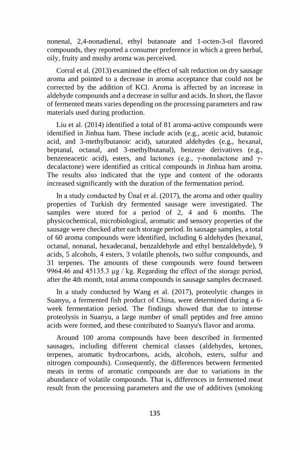
135
nonenal, 2,4-nonadienal, ethyl butanoate and 1-octen-3-ol flavored
compounds, they reported a consumer preference in which a green herbal,
oily, fruity and mushy aroma was perceived.
Corral et al. (2013) examined the effect of salt reduction on dry sausage
aroma and pointed to a decrease in aroma acceptance that could not be
corrected by the addition of KCl. Aroma is affected by an increase in
aldehyde compounds and a decrease in sulfur and acids. In short, the flavor
of fermented meats varies depending on the processing parameters and raw
materials used during production.
Liu et al. (2014) identified a total of 81 aroma-active compounds were
identified in Jinhua ham. These include acids (e.g., acetic acid, butanoic
acid, and 3-methylbutanoic acid), saturated aldehydes (e.g., hexanal,
heptanal, octanal, and 3-methylbutanal), benzene derivatives (e.g.,
benzeneacetic acid), esters, and lactones (e.g., γ-nonalactone and γ-
decalactone) were identified as critical compounds in Jinhua ham aroma.
The results also indicated that the type and content of the odorants
increased significantly with the duration of the fermentation period.
In a study conducted by Ünal et al. (2017), the aroma and other quality
properties of Turkish dry fermented sausage were investigated. The
samples were stored for a period of 2, 4 and 6 months. The
physicochemical, microbiological, aromatic and sensory properties of the
sausage were checked after each storage period. In sausage samples, a total
of 60 aroma compounds were identified, including 6 aldehydes (hexanal,
octanal, nonanal, hexadecanal, benzaldehyde and ethyl benzaldehyde), 9
acids, 5 alcohols, 4 esters, 3 volatile phenols, two sulfur compounds, and
31 terpenes. The amounts of these compounds were found between
9964.46 and 45135.3 µg / kg. Regarding the effect of the storage period,
after the 4th month, total aroma compounds in sausage samples decreased.
In a study conducted by Wang et al. (2017), proteolytic changes in
Suanyu, a fermented fish product of China, were determined during a 6-
week fermentation period. The findings showed that due to intense
proteolysis in Suanyu, a large number of small peptides and free amino
acids were formed, and these contributed to Suanyu's flavor and aroma.
Around 100 aroma compounds have been described in fermented
sausages, including different chemical classes (aldehydes, ketones,
terpenes, aromatic hydrocarbons, acids, alcohols, esters, sulfur and
nitrogen compounds). Consequently, the differences between fermented
meats in terms of aromatic compounds are due to variations in the
abundance of volatile compounds. That is, differences in fermented meat
result from the processing parameters and the use of additives (smoking

136
and seasoning), and the variety of aroma active compounds, such as the
presence of phenolic and terpene compounds (Flores and Olivares, 2015).
3.1 Aldehydes
Aldehydes are one of the most important chemical groups in fermented
sausage aroma and are formed as a result of the breakdown of
hydroperoxides. Aldehydes formed by fatty acid oxidation have a great
influence on the overall aroma of meat products due to the typical aroma
and low scent threshold. In fermented meat products, mainly hexanal, and
generally pentanal, octanal and 2-nonanal compounds are detected
(Ercoşkun et al., 2004; Marco et al., 2007). As the fermentation period
extends, the amount of aldehyde increases, and this compound has an effect
on the aroma of meat even at low concentrations (Kaban and Kaya 2007).
Aldehydes generally add scents of green plants, cut grass and greasy to
foods (Kesen et al., 2014). While 2-heptenal in meat products causes a
dense mold scent, while nonanal, 4-heptenal, 2,4 decadienal lead to oily,
stale, and unpleasant scents. Benzaldehyde compounds support the desired
fermented meat flavor (Ercoşkun and Ertaş, 2003; Flores and Olivares,
2015; Gandemer, 2002; Gök, 2006). The aromatic compounds included in
the aldehydes group in fermented meat products and their sensory
descriptions are given in Table 1 (Flores and Olivares, 2015).
Table 1 The aromatic compounds included in the aldehydes group in
fermented meat products and their sensory descriptions
Aldehyde Sensory descriptors
Hexanal Vegetables, fresh-cut grass, green
2-Hexenal Cooked potatoes, salty meat, meat broth
Pentanal Synthetic, green leaf, rancid
Octanal Geranium, floral, citrus, nettle, dry
Nonanal Herbal, geranium, nettle, dry, soap
2-Nonenal Cucumber, herbal, wood, caramel
2-Heptenal Rancid, dirty
4-Heptenal Nasty bread
2,4-Decadienal Fried, rancid, greasy
Benzaldehyde Fresh, pine, herbal, spices
Acetaldehyde Green
2-Methyl-butanal Bitter cheese, fruity, caramel, rancid
2-Methyl-propanal Fresh
Butanal Sweet, snacks

137
3.2 Ketones
Ketones formed by lipid oxidation are mainly methyl ketones. Possible
origins of methyl ketones are β-oxidation of free fatty acids by bacteria.
Therefore, the choice of starter culture affects the balance between the
oxidation products formed as a result of autoxidation of fatty acids and β-
oxidation. Ketones formed as a result of the oxidation of fats also
significantly affect the aroma in fermented meat products. Besides the
butter aroma produced by 2,3-butanedione (diacetyl), ketones exhibit very
variable flavor characteristics such as fruity, buttery or cheesy. In addition,
the formation of 1-octen-3-one in sausage increases during fermentation.
These compounds also create a metallic or mushroom-like flavor
(Ercoşkun and Ertaş, 2003; Ercoşkun et al., 2004; Flores and Olivares,
2015). The aromatic compounds included in the ketones group in
fermented meat products and their sensory descriptions are given in Table
2 (Flores and Olivares, 2015).
Table 2 The aromatic compounds included in the ketones group in
fermented meat products and their sensory descriptions
Ketones Sensory descriptors
2-Heptanone Nettle, fruity, medicinal
2,3-butanedione (diacetyl) Butter, cheese
2,3-Pentanedione Butter
3-Hydroxy-2-butanone Slight buttery
1-Octen-3-one Mushroom
3-Octen-2-one Mushroom, metali
2-Nonanone Herbal, mushroom, slight fruity
3.3 Terpenes
Terpenes produce herbal aromas such as resin, pine and herb. Limonene
is often found in fermented sausages that contain spices such as peppers,
and among them, linalool has also been described as a strong flavor active
compound. α-terpinen, which is included in the terpenes group and found
in pepper and some other spices, has also been identified in sausage
samples. Other terpenes identified in sausage are α-terpineol, β-pinene, β-
mircene, linalool, α-pinene, felandrene and 3-carene. It is stated that
terpenes constitute a significant part and even more than 50% of the
aromatic compounds obtained in some fermented meat products. For
example, Kaban (2010) states that the proportion of terpenes in sausage
samples varies between 56.11% and 76.32%. As a result of a study
conducted by Sezer Çelebi (2012), 34 terpenic compounds were detected
in sausage samples, and terpenes were found to be higher than other total

138
volatile compounds. The ratio of terpenes varies depending on the sausage
formulation. These differences may arise from the variety and amount of
spices used in production, as well as from the feed the animals eat (Demirel
and Gürler, 2017; Flores and Olivares, 2015; Kaban and Kaya, 2007;
Kaban, 2010). The aromatic compounds included in the terpenes group in
fermented meat products and their sensory descriptions are given in Table
3 (Flores and Olivares, 2015).
Table 3 The aromatic compounds included in the terpenes group in
fermented meat products and their sensory descriptions
Terpenes Sensory descriptors
Limonene Menthol, herbal, fresh, citric, orange
Linalool Intense floral, rose
Terpinene Herbal
Terpineol Green
β-Pinene Pungent
β-Mircene Lemon, fruity, green, herbal, spice
Felandrene Lemon, fruity, green
3-Carene Unpleasant
3.4 Aromatic Hydrocarbons
Phenolic compounds are characteristic in fermented smoked meats. For
this reason, most of the phenolic compounds have been detected in
Hungarian smoked salami. These 2-methoxy phenol (guaiacol) and 4-
methyl phenol are the strongest aromas (Flores and Olivares, 2015).
In fermented sausages, volatile phenol compounds can be of spice
origin. As a result of a study, it was determined that the sausage samples
contained volatile phenols such as methyl eugenol, eugenol and 2,4-bis-
1,1-dimethyl phenol, and their amounts varied between 143.51 and
2338.48 µg / kg (Ünal et al., 2017).
Aliphatic and aromatic hydrocarbons constitute another group of
volatile compounds identified in fermented sausages. In a study by Kaban
(2010), 10 aliphatic (0.14-8.03%) and 7 aromatic hydrocarbons (0.91-
12.17%) were determined in sausage samples. The sources of these
compounds vary widely. Aliphatic hydrocarbons, which are secondary
products of lipid oxidation, do not make a significant contribution to the
aroma due to their high sensory threshold. Aromatic hydrocarbons, on the
other hand, are more effective on aroma. Among aromatic hydrocarbons,
toluene (methyl benzene) can be caused by compounds formed as a result
of lipid breakdown. This compound is also found in herbs used as animal
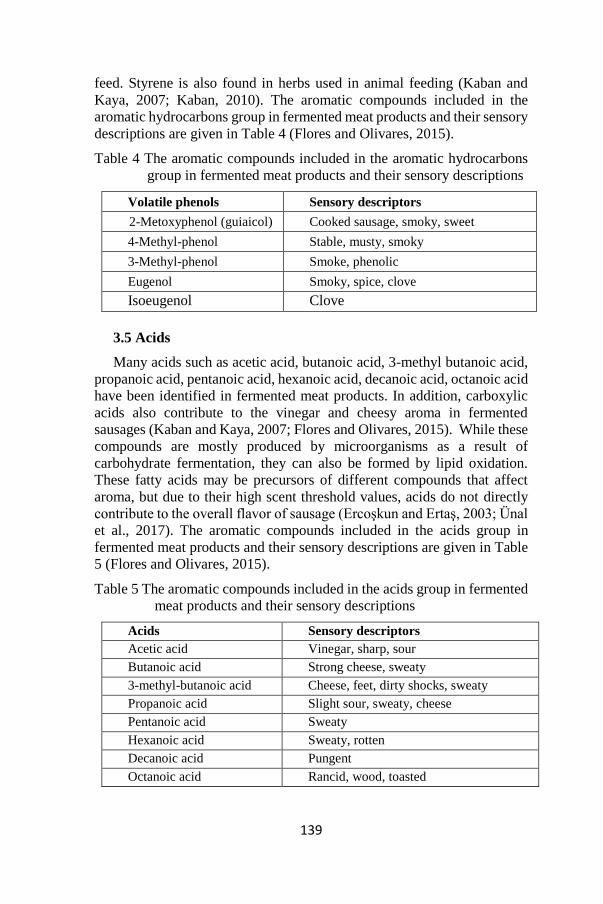
139
feed. Styrene is also found in herbs used in animal feeding (Kaban and
Kaya, 2007; Kaban, 2010). The aromatic compounds included in the
aromatic hydrocarbons group in fermented meat products and their sensory
descriptions are given in Table 4 (Flores and Olivares, 2015).
Table 4 The aromatic compounds included in the aromatic hydrocarbons
group in fermented meat products and their sensory descriptions
Volatile phenols Sensory descriptors
2-Metoxyphenol (guiaicol) Cooked sausage, smoky, sweet
4-Methyl-phenol Stable, musty, smoky
3-Methyl-phenol Smoke, phenolic
Eugenol Smoky, spice, clove
Isoeugenol Clove
3.5 Acids
Many acids such as acetic acid, butanoic acid, 3-methyl butanoic acid,
propanoic acid, pentanoic acid, hexanoic acid, decanoic acid, octanoic acid
have been identified in fermented meat products. In addition, carboxylic
acids also contribute to the vinegar and cheesy aroma in fermented
sausages (Kaban and Kaya, 2007; Flores and Olivares, 2015). While these
compounds are mostly produced by microorganisms as a result of
carbohydrate fermentation, they can also be formed by lipid oxidation.
These fatty acids may be precursors of different compounds that affect
aroma, but due to their high scent threshold values, acids do not directly
contribute to the overall flavor of sausage (Ercoşkun and Ertaş, 2003; Ünal
et al., 2017). The aromatic compounds included in the acids group in
fermented meat products and their sensory descriptions are given in Table
5 (Flores and Olivares, 2015).
Table 5 The aromatic compounds included in the acids group in fermented
meat products and their sensory descriptions
Acids Sensory descriptors
Acetic acid Vinegar, sharp, sour
Butanoic acid Strong cheese, sweaty
3-methyl-butanoic acid Cheese, feet, dirty shocks, sweaty
Propanoic acid Slight sour, sweaty, cheese
Pentanoic acid Sweaty
Hexanoic acid Sweaty, rotten
Decanoic acid Pungent
Octanoic acid Rancid, wood, toasted

140
3.6 Alcohols
Alcohols in fermented meats are usually caused by lipid oxidation.
However, they can also occur as a result of carbohydrate metabolism and
amino acid catabolism. In general, alcohol compounds have not been
identified as important aromatic contributors in fermented sausages. This
may be due to the high detection threshold of alcohol compounds. In his
study, Kaban (2010) detected seven different alcohols in sausage, and the
only alcohol determined in all of the samples examined was
benzenemethanol, 4- (1-methylethyl). Aliphatic linear alcohols generally
are formed by degradation of lipid hydroperoxides. Branched alcohols can
be formed from amino acids by Strecker degradation (Flores and Olivares,
2015; Kaban and Kaya, 2007; Kaban, 2010; Ünal et al., 2017). The
aromatic compounds included in the alcohols group in fermented meat
products and their sensory descriptions are given in Table 6 (Flores and
Olivares, 2015).
Table 6 The aromatic compounds included in the alcohols group in
fermented meat products and their sensory descriptions
Alcohols Sensory descriptors
Ethanol Baker’s bread, yeast
1-Propanol Fresh, herbal
1-Pentanol Toasted, toasted meat, pine
1-Octen-3-ol Mushroom
1-Hexanol Green grass, plastic
2-Heptanol Plastic, pork scratchings
3.7 Esters
Many ester compounds have been identified as responsible for fruity
and caramel aromas in fermented sausages. Most of the esters are ethyl
esters. Among them, the ones with the strongest aromas are ethyl
butanoate, ethyl 2-methyl-butanoate and ethyl pentanoate. The formation
of esters in fermented meat products depends more on microbial factors
compared to other reactions. Due to their low scent thresholds and well-
known effects on the overall flavor of food products, esters are remarkable
aroma compounds that provide sausage samples with a fruity and pleasant
aroma (Ercoşkun and Ertaş, 2003; Flores and Olivares, 2015; Ünal et al.,
2017). The aromatic compounds included in the esters group in fermented
meat products and their sensory descriptions are given in Table 7 (Flores
and Olivares, 2015).

141
Table 7 The aromatic compounds included in the esters group in fermented
meat products and their sensory descriptions
Esters Sensory descriptors
Ethyl butanoate Fruity, caramel, pineapple, strawberry
Ethyl 2-Methyl-butanoate Sweet, pineapple, fruity, strawberry
Ethyl Pentanoate Fruity, strawberry
Ethyl 2-Methyl-propanoate Pineapple, strawberry, fruity, caramel
Propyl acetate Apple, caramel, fruity, floral
Methyl butanoate Fruity, floral
2-methyl-propyl acetate Fruity
3.8 Sulfur and Nitrogen Compounds
Sulfur compounds are characterized by low threshold values and the
characteristic aroma defined as garlic, onion, cooked potatoes and
sometimes cooked meat. The strongest scents reported in fermented meats
are diallyl sulfide, diallyl disulfide, dimethyl disulfide, methional (3-
methylthiopropanal) and methanethiol (Flores and Olivares, 2015).
Compounds containing different proportions and types of sulfur have been
identified in fermented meat products. Kaban (2010) identified 11 sulfur
compounds in sausage in his study and stated that most of these compounds
originated from the spices used in the formulation, especially garlic (Kaban
and Kaya, 2007; Kaban, 2010). The aromatic compounds included in the
sulfur group in fermented meat products and their sensory descriptions are
given in Table 8 (Flores and Olivares, 2015).
Table 8 The aromatic compounds included in the sulfur group in fermented
meat products and their sensory descriptions
Sulfur compounds Sensory descriptors
Diallyl sulfide Garlic
Diallyl disulfide Garlic
Dimethyl disulfide Garlic, caramel, toasted
Methional Cooked potato, brothy, rancid
Methanethiol Rotten eggs, coliflower, unpleasant
Methyl-allyl sulfide Onion, unpleasant, garlic
2-Methyl-3-furyl disulfide Cooked meat
Nitrogenous compounds are commonly defined as small flavor
compounds in cooked meat due to their characteristic fried and nut aroma.
Also, 2-acetyl-pyrroline has been described as one of the strongest aromas
in fermented sausages. Among the nitrogenous compounds, there are
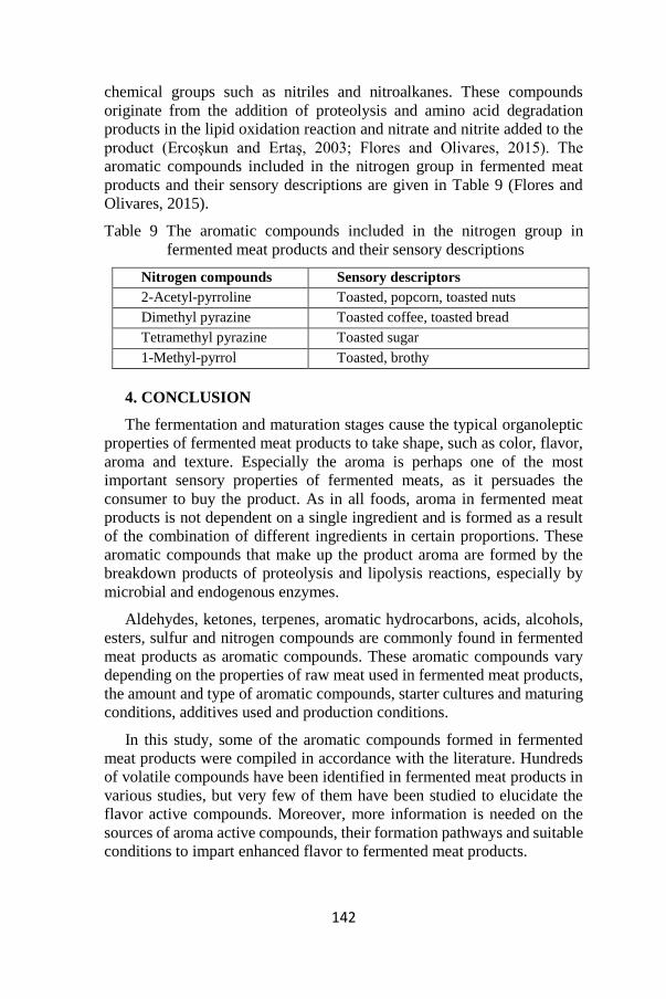
142
chemical groups such as nitriles and nitroalkanes. These compounds
originate from the addition of proteolysis and amino acid degradation
products in the lipid oxidation reaction and nitrate and nitrite added to the
product (Ercoşkun and Ertaş, 2003; Flores and Olivares, 2015). The
aromatic compounds included in the nitrogen group in fermented meat
products and their sensory descriptions are given in Table 9 (Flores and
Olivares, 2015).
Table 9 The aromatic compounds included in the nitrogen group in
fermented meat products and their sensory descriptions
Nitrogen compounds Sensory descriptors
2-Acetyl-pyrroline Toasted, popcorn, toasted nuts
Dimethyl pyrazine Toasted coffee, toasted bread
Tetramethyl pyrazine Toasted sugar
1-Methyl-pyrrol Toasted, brothy
4. CONCLUSION
The fermentation and maturation stages cause the typical organoleptic
properties of fermented meat products to take shape, such as color, flavor,
aroma and texture. Especially the aroma is perhaps one of the most
important sensory properties of fermented meats, as it persuades the
consumer to buy the product. As in all foods, aroma in fermented meat
products is not dependent on a single ingredient and is formed as a result
of the combination of different ingredients in certain proportions. These
aromatic compounds that make up the product aroma are formed by the
breakdown products of proteolysis and lipolysis reactions, especially by
microbial and endogenous enzymes.
Aldehydes, ketones, terpenes, aromatic hydrocarbons, acids, alcohols,
esters, sulfur and nitrogen compounds are commonly found in fermented
meat products as aromatic compounds. These aromatic compounds vary
depending on the properties of raw meat used in fermented meat products,
the amount and type of aromatic compounds, starter cultures and maturing
conditions, additives used and production conditions.
In this study, some of the aromatic compounds formed in fermented
meat products were compiled in accordance with the literature. Hundreds
of volatile compounds have been identified in fermented meat products in
various studies, but very few of them have been studied to elucidate the
flavor active compounds. Moreover, more information is needed on the
sources of aroma active compounds, their formation pathways and suitable
conditions to impart enhanced flavor to fermented meat products.

143
References
Başyiğit, G., Karahan, A.G. and Kılıç, B. (2007). Functional starter
cultures and probiotics in fermented meat products. Turkish Journal of
Hygiene and Experimental Biology, 64 (2), 60-69.
Casaburi, A., Di Monaco, R., Cavella, S., Toldrá, F., Ercolini, D. and
Villani, F. (2008). Proteolytic and lipolytic starter cultures and their
effect on traditional fermented sausages ripening and sensory traits.
Food Microbiology, 25(2), 335-347.
Corral S, Salvador A. and Flores, M. (2013). Salt reduction in slow
fermented sausages affects the generation of aroma active compounds.
Meat Science, 93, 776–785.
Demirel, N.Y. and Gürler, Z. (2017). Investigation of the effect of
microorganism combinations used in fermented sausage production on
flavor development. Eurasian Journal of Veterinary Sciences, 33 (1),
34-39.
Ercoşkun, H. and Ertaş, A.H. (2003). Flavor components and formation of
fermented meat products. Journal of Food Engineering, 7 (16), 38-44.
Ercoşkun, H., Kiralan, M. and Işıksal, S. (2004). Lipid reactions in
fermented meat products. Food Engineering Journal, 8 (18), 38-46.
Flores, M., Soler, C., Aristo, M.C. and Toldra, F. (2006). Effect of brine
thawing/salting for time reduction in spanish dry cured ham
manufacturing on proteolysis and lipolysis during salting and post-
salting periods. Eur. Food Res. Technol., 222, 509-515.
Flores, M. and Olivares, A. (2015). Flavor. F. Toldrá, Y. Hui, I. Astiasarán,
J. Sebranek, R. Talon, Handbook of Fermented Meat and Poultry (
s.217-225), Wiley Online Library.
Gandemer, G. (2002). Lipids in muscles and adipose tissues, changes
during processing and sensory properties of meat products. Meat
Science, 62(3), 309-321.
Gök, V. (2006). Effects of antioxidant use on some quality properties of
fermented sausages (Doctoral Thesis). Ankara University, Institute of
Science, Ankara.
Gökalp, H.Y., Ercoşkun, H. and Çon A.H. (1998). Some biochemical
reactions and effects on aroma in fermented meat products. Pamukkale
University Faculty of Engineering, Journal of Engineering Sciences, 3
(4), 805-811.

144
Kaban, G. and Kaya, M. (2007). Volatile compounds in fermented
sausages. Atatürk University, Faculty of Agriculture, 38 (2), 225-230.
Kaban, G. (2010). Volatile compounds of traditional turkish dry fermented
sausage (sucuk). International Journal of Food Properties, 13(3),525-
534.
Kaban, G. and Kaya, M. (2011). Volatile compounds of traditionally
produced pastırma. Fleıschwırtschaft, 91(4),112-116.
Kesen, S., Kelebek, H. and Selli, S. (2014). Characterization of the key
aroma compounds in Turkish olive oils from different geographic
origins by application of aroma extract dilution analysis (AEDA).
Journal of Agricultural and Food Chemistry, 62(2), 391-401.
Laslo, É., György, É. and Czikó, A. (2019). Meat starter cultures: Isolation
and characterization of lactic acid bacteria from traditional sausages.
Acta Universitatis Sapientiae Alimentaria, 12(1), 54-69.
Liu, X.S., Liu, J.B., Yang, Z. M., Song, H.L., Liu, Y. and Zou, T.T. (2014). Aroma-active compounds in jinhua ham produced with different
fermentation periods. Molecules, 19(11), 19097-19113.
Macedo, R.E.F., Luciano, F.B., Cordeiro, R.P. and Udenigwe, C.C. (2017).
Sausages and other fermented meat products. Starter Cultures in Food
Production, Ed: Speranza, B., Bevilacqua, A., Corbo, M. R.,
Sinigaglia, M. Wiley-Blackwell, Chichester, 324-354.
Marco, A., Navarro, J.L. and Flores, M. (2007). Quantification of selected
odor-active constituents in dry fermented sausages prepared with
different curing salts. Journal of Agricultural and Food Chemistry,
55(8), 3058–3065.
Martín-Sánchez, A.M., Chaves-López, C., Sendra, E., Sayas, E.,
Fenández-López, J. and Pérez-Álvarez, J. Á. (2011). Lipolysis,
proteolysis and sensory characteristics of a Spanish fermented dry-
cured meat product (salchichón) with oregano essential oil used as
surface mold inhibitor. Meat Science, 89(1), 35-44.
Olivares, A., Navarro, J.L. and Flores, M. (2011). Effect of fat content on
aroma generation during processing of dry fermented sausages. Meat
Science, 87(3), 264-273.
Ojha, K.S., Kerry, J.P., Duffy, G., Beresford, T. and Tiwari, B.K. (2015).
Technological advances for enhancing quality and safety of fermented
meat products. Trends in Food Science & Technology, 44(1), 105-116.

145
Öziş, G. (2014). The Effects of some organic acids and their salts on some
properties of fermented sausage (Master Thesis). Abant İzzet Baysal
University, Institute of Science, Bolu.
Öztan, A. (1999). Meat Science and Technology, 3rd Edition, Hacettepe
University Publications, Ankara.
Resconi, V.C., Escudero, A. and Campo, M.M. (2013). The development
of aromas in ruminant meat. Molecules,18(6), 6748-81.
Rotsatchakul, P., Visesanguan, W., Smitinont, T. and Chaiseri, S. (2009).
Changes in volatile compounds during fermentation of nham (Thai
fermented sausage). International Food Research Journal, 16, 391-
414.
Serdaroğlu, M. and Tömek, S. (1995). The importance of proteolytic
enzymes in fermented meat products. Pamukkale University Faculty of
Engineering, Journal of Engineering Sciences, 3(1), 89-94.
Sezer Çelebi, Y. (2012). Determination of the potential use of some lactic
acid bacteria isolated from fermented sausage as starter culture (Master
Thesis). Erciyes University, Institute of Science, Kayseri.
Şanes, A. (2006). Production of functional (diet) sausage with reduced
calories and fat (Master Thesis). Istanbul Technical University, Institute
of Science, Istanbul.
Toldra, F. (1998). Proteolysis and lipolysis in flavour development of dry-
cured meat products. Meat Science, 49(1), 101-110.
Toldra, F., Sanz, Y. and Lores, M. (2001). Meat Fermentation
Technology, In Hui, Y.H. Ed.. Meat Science Applications. Marcel
Dekker Incorporated, New York, USA.
Ulusoy, B.H. (2007). Production of fermented sausage with kefir culture
(PhD Thesis). Istanbul University, Institute of Health Sciences,
Istanbul.
Ünal, E., Erginkaya, Z. and Selli, S. (2017). The effect of
microencapsulated Lactobacillus rhamnosus and storage period on
aroma properties of Turkish dry-fermented sausage (sucuk). Journal Of
Food Measurement And Characterızatıon, 1(1),1-11.
Van Ba, H., Hwang, I., Jeong, D. and Touseef, A. (2012). Principle of meat
aroma flavors and future prospect. Latest research into quality control,
Ed: Akayar, I. Intech Open Access Publisher, London, 145–176.
Wang, W., Xia, W., Gao, P., Xu, Y. and Jiang, Q. (2017). Proteolysis
during fermentation of Suanyu as a traditional fermented fish product
of China. International Journal of Food Properties, 20(1), S166-S176.

146
Yetim, H. (2013). Isolation, identification and determination of important
technological and functional properties of yeast in traditional fermented
sausages for use as starter culture. Erciyes University Scientific
Research Projects Coordination Unit, Kayseri.
Yılmaz, İ. and Velioğlu, H.M. (2009). Fermented meat products. Quality
of Meat and Meat Products. Transworld Research Network, 99-114.
Zanardi, E., Ghidini, S., Battaglia, A. and Chizzolini, R. (2004). Lipolysis
and lipid oxidation in fermented sausages depending on different
processing conditions and different antioxidants. Meat Science, 66 (2),
415-423.
147
CHAPTER IX
BUILDING SCIENCE I EXPERIENCES AS AN APPLIED
COURSE ON EMERGENCY REMOTE TEACHING
(ERT) OF ARCHITECTURE
Seher GÜZELÇOBAN MAYUK
(Asst. Prof. Dr.); Gebze Technical University, Kocaeli, Turkey;
[email protected]; Orcid: 0000-0002-2676-4784
Elif ÖZER YÜKSEL
(Asst. Prof. Dr.); Gebze Technical University, Kocaeli, Turkey;
[email protected]; Orcid: 0000-0002-1041-8748
N. Özge ESENER
(Res. Asst.); Gebze Technical University, Kocaeli, Turkey;
[email protected]; Orcid: 0000-0002-3949-068X
Gizem ASLAN
(Res. Asst.); Gebze Technical University, Kocaeli, Turkey;
[email protected]; Orcid: 0000-0002-0430-5106
Merve ÖZDOĞAN
(Res. Asst.); Gebze Technical University, Kocaeli, Turkey;
[email protected]; Orcid: 0000-0002-6643-1749
Çetin SÜALP
(Res. Asst.); Gebze Technical University, Kocaeli, Turkey;
[email protected]; Orcid: 0000-0002-1227-7774
1. Introduction
The Covid-19 pandemic emerged in mid-March 2020 in Turkey when
were the early days of the spring semester. After this time, all schools and
universities were being announced to close and the rapid transition of
education has started to online and digital education formats for adopting
remote modes of teaching and learning (Green et al., 2020). Well-planned
online learning experiences are meaningfully different from courses
offered online in response to a crisis or disaster (Hodges et al., 2020). As a
frontline emergency service, this educational transition method with

148
remote learning and educational technologies repositioned is named as an
emergency remote teaching (ERT) method (Green et al., 2020).
Yıldırım (2020) said that the remote education had started with letters
in the 1700s. It shows that the embedding of digital technologies as part of
educational practices is neither new nor unique to the global pandemic
(Green et al., 2020). However, it can be said that the use of ERT in
architecture education has no longer time. When the literature is reviewed,
many studies are encountered on subjects such as emergency remote
teaching and distance education (Dikmen and Bahçeci, 2020; Durak et al.,
2020; Green et al., 2020; Hodges et al., 2020; Keskin and Özer Kaya, 2020;
Whittle et al., 2020; Yıldırım, 2020; Yılmaz İnce et al., 2020). Kauser
(2020) can be reached as a resource on emergency remote teaching (ERT)
of architecture. In this sense, it can be said that there is a deficiency in the
literature about teaching with ERT in architecture.
Conventionally architecture education is going by interactive ways.
Especially at design studios, it includes a group working with collaborative
teaching and learning for developing students’ creative skills. Because of
this, the students need to interact or discuss together with their teachers and
other students (Kauser, 2020). For this reason, examining the use of ERT
in architecture education is necessary for these Covid-19 pandemic
conditions. In addition to this, it can be also said that the use of ERT in
applied courses is a difficult method. Building science courses in
architecture education, which are applied courses, have two main parts.
One of them is theory and the other is practice. It can be said that the ERT
method is more suitable for the theory part rather than practice.
On the other hand, the features of the generation gain importance in the
methods to be used in today's learning environment (Güzelçoban Mayuk
and Coşgun, 2020). Generation Z individuals, who were born after 2000s,
take part as learners in building science courses nowadays. Generation Z
is also referred to by various names such as “internet generation, digital
generation, millennium generation” because of their born age’s features.
They are said to be individuals who integrate technology with their lives,
have social network affiliations, have a fondness for virtual games, have
an interest in global issues and have high adaptability. It is also mentioned
that they are open to innovation, optimistic, talented, goal-oriented, well-
educated, self-confident, easily bored and capable of performing multiple
skills simultaneously (Erden, 2017). The individuals of this generation are
stated as individuals who learn knowledge fast, prefer graphic expression,
prioritize winning and are competitive (Ardıç and Altun, 2017). Based on
these features, it can be said that digital learning brought about by the
Covid-19 period is compatible with the educational methods of generation

149
Z. It is known that one of these education methods is learning by doing
method (Güzelçoban Mayuk and Coşgun, 2020). Learning by doing is a
method to facilitate learning activity. In this method, all educational
periods need to look, feel and be done as they are in real life (Erkan Yazıcı
and Töre, 2014).
Within the scope of the study, the methods for the functioning of the
Building Science I (BS I) course in the Covid-19 period were explained.
BS I is a compulsory course in the curriculum of Gebze Technical
University (GTU) Department of Architecture in the spring term and
generation Z individuals take part as learners at this course on 2020 spring
term. For this reason, the learning by doing method is used in this course
on spring. The survey results at the end of the 2020 spring term conducted
with the students taking the course were included in the study and the
opinions of the students about the period and method were evaluated by
this way. About GTU BS I course, the methodology of the course in the
Covid-19 period and the evaluation survey and its results are given as parts
of the study. It is completed with the conclusion part in accordance with
the findings and discussion part.
2. About GTU Building Science I Course
Building Science I (BS I) is an ARCH 142 coded and compulsory
undergraduate course, maintained in the second semester (spring) of the
first year in architecture education at GTU. As of the 2017-2018 academic
year, according to the updated course plan; BS I has 5 ECTS credits and 4
hours (2 hours of theory + 2 hours of practice + 0 hours of laboratory) a
week. The requirement for the student attendance at the course is consisting
of both theory and practice as 80 percentage.
The course requires face-to-face interaction. In the first two hours of
the course, the lecturer gives theoretical information about building
elements. Then he/she gives information about the homework or
assignment (in-class practice work) of the week. Afterwards, the research
assistants of the course help students with drawings and models during the
in-class practice phase of the course. Assignments (in-class works),
homeworks, exams, term projects (models, research projects) done during
the semester are evaluated for the final gradation of course.
BS I is one of the fundamental courses of architectural education in
GTU. In this course, the student learns the building components and the
integration principles of components. Application assignments are
significantly useful in this learning period. Through these assignments, the
student learns to solve the structural problems encountered in project
production phases.

150
The course includes that the explanations and applications of the basic
principles of building science. It also includes the headings of the design
of sub-systems, building foundations, walls, floors and joinery building
elements. In addition to the theoretical explanations on reinforced concrete
skeletal system and masonry building construction systems, wood and steel
structural systems are included in the last weeks of the course.
The course continues with the course of Building Science II in the
following semester at GTU. In BS II, theoretical information and various
application assignments about vertical circulation tools and roof systems
are given.
2.1 The Methodology of the BS I Course
In the past, mainly drawing and model assignments were used in GTU
building science courses, but recently, education has been adapted for
generation Z. In this period, the student is directed to do lots of research.
Considering the close relationship of generation Z with technology, it is
useful to push the student to find the right up-to-date information in the
light of the knowledge he/she gained in the course and let him/her figure
out how to solve the problem. In this way, it is hoped that the student will
be able to develop creative architectural solutions for the problems he/she
encounters in business life with his/her research skills and knowledge.
To adapt the education system to generation Z, the ‘learning by doing’
method has been prioritized. In this method, students are provided to
develop their work with research based on the information they have
acquired in the course and to produce models in desired scales. In this way,
it is aimed for them to learn the theory and practice by experiencing. The
models produced are considered as term projects. Model deliveries are
completed with daily detail workshops. In this way, it is aimed that students
will develop their integrated thinking skills in a more flexible production
environment (Güzelçoban Mayuk and Coşgun, 2020).
Students who have developed problem-solving and integrated thinking
skills can use the knowledge and skills they have learned in the BS I course
in other undergraduate courses as well. Thus, it has been ensured that the
BS I course is also integrated into the Architectural Design Studio course.
For a holistic architectural education, importance has been placed on the
synchronization of these two courses and their feeding each other.
2.2 The Methodology of the Course in the Covid-19 Period at 2019-
20 Spring Semester
Arch 142 Building Science I was conducted in the 2019-2020 Spring
Semester with Covid-19 conditions. The courses are conducted with a

151
group of faculty members, which vary according to the semesters. In the
lessons, theoretical information is conveyed mostly by the lecturer and the
courses are completed with the applications carried out by the research
assistants. The BS I course in the spring semester of 2019-2020 was
conducted with two faculty members and four research assistants; a total
of 78 students attended to the course.
In this context, the education, which was carried out face-to-face in the
first four weeks of the term, was carried out with emergency remote
education until the end of the term after a two-week break due to Covid-19
measures. BS I courses, which consist of theory and practice sections, were
carried out simultaneously and asynchronously with the MS Teams
program during the emergency remote education period. For this reason,
the total number of applications and assignments during the term has been
reduced. The updated workplan for the spring term of the course is
included in Table 1.
The theory section of the course carried out with the presentations made
by lecturers. Meanwhile, presentations were recorded. Thus, in addition to
being able to follow the presentations by students simultaneously and
students were provided to access the theoretical information of the
concerned course at the end. For this purpose, course folders were created
in the general channel where simultaneous courses are conducted in MS
Teams. By this way, the access of all course documents was provided.
The application section of the course was carried out under the control
of research assistants. Before the concerned week of the course, the
theoretical presentation and application files of that week were uploaded
to the application group channels opened in MS Teams by the research
assistant of each group and the students were made ready for the course. In
the education before Covid-19, the applications which in face-to-face were
continued in the class after the theoretical presentations were turned into
weekly assignments during the emergency remote teaching period. At the
end of each simultaneous course, the assessment of the previous week’s
application stage was made and then the desired criteria were explained on
the application of that week. In this stage, it is expected from students to
upload the applications given as an assignment to the concerned folders of
the group channels in MS Teams on the specified day and time. The
assignments of the concerned week were graded in written explanations
according to the required criteria by the research assistants carrying out
each application group and announced to the students through the same
channel. No restrictions were placed on the method of the application
drawings of the students. They were expected to upload photographs of

152
their hand drawings or drawings made by using the other digital platforms
to concerned MS Teams channel in desired formats.
Table 1 The workplan of the course in 2019-20 spring semester.
ARCH 142 BUILDING SCIENCE I
2019-2020 SPRING SEMESTER PLAN
WEEKS CONTENTS METHODS
Week 1
Introduction and general information about the
method and the scope of the lecture, conceptual
definitions.
Face-to-Face Teaching
Week 2
Foundation systems
Practice 1
Assignment 1
Face-to-Face
Teaching
Week 3
Carcass system foundations
Practice 2
Assignment 2
Face-to-Face Teaching
Week 4 Raft foundation, insulation against water and humidity, the elements of carcass system
Practice 3
Face-to-Face
Teaching
Week 5 Break of Covid-19 No Course
Week 6 Break of Covid-19 No Course
Week 7 Online Trial Course Wall sytems
Practice 4 // Assignment 4
Emergency Remote
Teaching (ERT)
Week 8
Floor systems Term Project: Assignment of Research Project and
Groups
Practice 5 // Assignment 5
ERT
Week 9
Arch, vault, dome systems
Practice 6 // Assignment 6
Assessment for the Term Project
ERT
Week 10 Door and window system components
Practice 7 // Assignment 7 ERT
Week 11 Door and window system components
Practice 8 // Assignment 8 ERT
Week 12 Wood and steel construction systems
Practice 9 // Assignment 9
Assessment for the Term Project review
ERT
Week 13 Term Project Presentations- Project Delivery ERT
Week 14 No Course (because of the date) No Course
In addition to drawing the applications given as assignment during the
application period in consultation with the concerned research assistant, it

153
was aimed that the students to research and make a literature review
individually. It is aimed for students to turn the period into an opportunity
and improve their learning skills with this application method emerged due
to Covid-19. In this respect, it was ensured that students experienced the
digital technology as a learning tool, which they started to use in the early
stage of architecture education with the BS I course during the Covid-19.
In the exam stages, that could not carry out face to face, are integrated
into emergency remote teaching in this period, and solutions have been
applied to increase research, experience, and integration. Exams were
conducted as follows:
In the mid-term exam, a research assignment was given to students to
question, consolidate, and develop the information, which they achieved
as a result of theoretical and applied training. In the related assignment; the
students were expected to prepare a report by examining and analyzing
from the site plan to the system details of a building, which they chose, in
groups of 3-5, using the literature review method. In the report, the
examination of the buildings has been requested to be made within the titles
such as; general information about the building, site plan and layout
decisions, construction system, structural elements, evaluation and result
and bibliography. In addition to this report, students were expected to
submit the results of their research as a five-minute video in which they
presented as a group. The prepared video was watched simultaneously, and
an environment was created in which the students would answer the
questions to be asked. Assignments, which submitted on the online
platform until the specified date, were evaluated with the criteria of the
video and simultaneous presentation, the submitted reports and the
suitability of the reports for the assignment.
In the final assignment, it is aimed that the students consolidate the
knowledge they have acquired in the BS I course through the projects
which they produce in the Architectural Design studios. In the assignment
to be done individually, the students were asked to draw a part of their
projects, carried out in the Architectural Design studios in the spring
semester of 2019-2020, at 1/20 scale. Within the extent of the assignment,
it is expected that the site plan, floor plans, sections and elevations will be
submitted to understand their projects designed in studios. In the project of
BS I final assignment, it was requested to submit 1/20 system detail
drawings including plan-section-elevation of the partial sections which are
selected with the lecturers. Grading of the assignments was made
according to the evaluation criteria such as project submission, page layout
and the conformity of the plan-section-elevations in the system detail to
1/20 scale.

154
As a make-up assignment, it was requested to submit a revised and
detailed version of the assignment which made according to the critics
given in the final assignment evaluation. The make-up assessment criteria
were the same as those specified in the final assignment.
3. The Evaluation Survey and Its Results
70 students passed successfully of Arch 142 Building Science I course
from the registered 78 students in the term of spring 2020. At the end of
the semester, an evaluation survey was prepared over MS Teams in order
to identify the deficiencies in lectures and also, to increase the quality of
the course. The acquisitions, positive and negative aspects of the course,
and their suggestions, if any, as well as their satisfaction level and their
remote or face-to-face training preferences were also asked by this survey.
33 students participated that the attendance of 42% in this 6-questioned
survey, which had 4 open-ended and 2 closed-ended questions. One of the
closed-ended questions was a rating scale and the other one was a nominal
question shown in Table 2.
Table 2 Ouestions of the evaluation survey for the BS I Course in
Spring 2020
Question
number
Question
1. Can you convey your ACQUISITIONS from the Spring 2020 term of Arch
142 Building Science I course in three (3) words?
(For example: research skill, teamwork, program planning…etc.)
2. Could you tell us about the POSITIVE aspects of Arch142 Building Science I course about Spring 2020 term in three (3) words?
(For example: lively, actual, lifelike)
3. Could you tell us about the NEGATIVE aspects of Arch 142 Building Science I course about Spring 2020 term in three (3) words?
(For example: none :))
4. Are you satisfied that Arch 142 Building Science I course has been
conducted with remote education in Spring 2020?
(5 very satisfied, 4 satisfied, 3 neutral, 2 unsatisfied, 1 very unsatisfied)
5. Arch 142 Building Science I course will be more efficient for Fall 2020
semester as .........
a. Face-to-face education
b. Remote education
c. Both
6. What are your SUGGESTIONS, if any, of Arch 142 Building Science I course for Spring 2021?

155
The first open-ended question was replied with a rate of 70% by 32
students with 67 of 96 (32x3) statements. ‘Research & report skill’ was the
prevalent opinion with 34% for the first question as an acquisition.
‘Teamwork’, ‘program planning’ and ‘digital drawing skill’ were the
following answers with respectively 21, 16 and 11%. The second open-
ended question was answered with a rate of 54% by 29 students with 47 of
87 (29x3) statements. ‘Instructive and technical’ was the common answer
as a positive aspect with 23%. ‘Attractive and enjoyable’, ‘realistic’ and
‘lecturers taking care of students’ were the following answers with
respectively 13, 11 and 11%. The third open-ended question was replied
with a rate of 48% by 28 students with 40 of 84 (28x3) statements. ‘Info
confusion / can't reach correct info’ was the common answer as a negative
aspect with 20%. ‘Too much course load’, ‘thinks he/she got an undeserved
grade’ and ‘none’ were the following answers with respectively 15, 13 and
10%. Some of the remarkable answers among the others were ‘to be able
to repeat lessons at any time thanks to the recording of lessons’ and
‘Remote education caused a fair environment because of the absence of the
noise in the classroom’.
The fourth open-ended question (the sixth one) was replied by 22
students with 32 suggestions. ‘Applied education should be increased’ was
a common suggestion with 22%. ‘The system that includes both training
methods should be widespread’, ‘syllabus should be updated’ and ‘course
load should be reduced’ were the following answers with respectively 13,
13 and 9%. Additionally, some of them have suggested that ‘online
submissions should be continued’ and ‘final, which was a research and
report homework, should be continued (Fig. 1).
Figure 1 Illustration of the open-ended questions data.
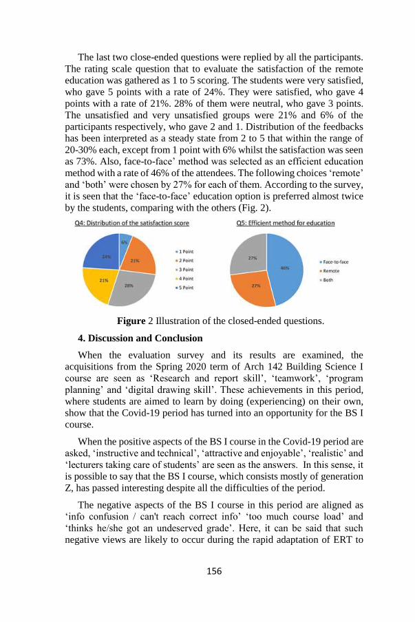
156
The last two close-ended questions were replied by all the participants.
The rating scale question that to evaluate the satisfaction of the remote
education was gathered as 1 to 5 scoring. The students were very satisfied,
who gave 5 points with a rate of 24%. They were satisfied, who gave 4
points with a rate of 21%. 28% of them were neutral, who gave 3 points.
The unsatisfied and very unsatisfied groups were 21% and 6% of the
participants respectively, who gave 2 and 1. Distribution of the feedbacks
has been interpreted as a steady state from 2 to 5 that within the range of
20-30% each, except from 1 point with 6% whilst the satisfaction was seen
as 73%. Also, face-to-face’ method was selected as an efficient education
method with a rate of 46% of the attendees. The following choices ‘remote’
and ‘both’ were chosen by 27% for each of them. According to the survey,
it is seen that the ‘face-to-face’ education option is preferred almost twice
by the students, comparing with the others (Fig. 2).
Figure 2 Illustration of the closed-ended questions.
4. Discussion and Conclusion
When the evaluation survey and its results are examined, the
acquisitions from the Spring 2020 term of Arch 142 Building Science I
course are seen as ‘Research and report skill’, ‘teamwork’, ‘program
planning’ and ‘digital drawing skill’. These achievements in this period,
where students are aimed to learn by doing (experiencing) on their own,
show that the Covid-19 period has turned into an opportunity for the BS I
course.
When the positive aspects of the BS I course in the Covid-19 period are
asked, ‘instructive and technical’, ‘attractive and enjoyable’, ‘realistic’ and
‘lecturers taking care of students’ are seen as the answers. In this sense, it
is possible to say that the BS I course, which consists mostly of generation
Z, has passed interesting despite all the difficulties of the period.
The negative aspects of the BS I course in this period are aligned as
‘info confusion / can't reach correct info’ ‘too much course load’ and
‘thinks he/she got an undeserved grade’. Here, it can be said that such
negative views are likely to occur during the rapid adaptation of ERT to

157
the period. At this point, efforts would be made for the solutions. In
addition, it is pleasing to receive the answer of none in the survey as a
negative opinion for the teachers.
The survey and its results show that there is a satisfaction generally with
the BS I course conducted in the period. In this sense, 73% of students who
score 3 and above appear to be. Some of the notable answers for this
satisfaction were ‘to be able to repeat lessons at any time thanks to the
recording of lessons’ and ‘remote education caused a fair environment
because of the absence of the noise in the classroom’. However, it is
concluded that 46% of the class preferred face-to-face training. It is thought
that the reason for this ratio may be the difficulties experienced in the
period, related to the negative aspects mentioned in the previous questions.
Some suggestions of the students in the evaluation survey for the other
BS courses in this Covid-19 period were specified as: ‘Applied education
should be increased’, ‘the system that includes both training methods
should be widespread’, ‘syllabus should be updated’ and ‘course load
should be reduced’. Additionally, ‘online submissions should be
continued’ and ‘final, which was a research and report homework, should
be continued because of quite instructive’ were some other suggestions.
According to these suggestions and also this study results, new work plans
for BS II courses in the fall term 2020 had been done.
It is also seen from the survey and results that the open-ended questions
asked to the students were answered less. It shows that the generation Z
members respond to optional questions and prefer to report their
suggestions quickly. It can be seen that this situation coincides with the
easily bored feature of generation Z. In order to solve this feature, it may
be useful to direct questions to students.
In conclusion, it can be said that it was determined that the BS I course
was conducted efficiently in the emergency remote teaching period. On the
other hand, face-to-face teaching was preferred by students more in applied
courses. In the Covid-19 period, which is expected to continue, it is
important to receive a lot of feedback as in this study to carry out the
applied lessons more efficiently.
Acknowledgements
We would like to thank all the students who participated to the Building
Science I course and evaluation survey in the 2019-20 spring term at Gebze
Technical University Department of Architecture.
Unless otherwise stated, the figures and tables used in the article belong
to the authors.

158
References
Ardıç, E, & Altun, A. (2017). Dijital Çağın Öğreneni. International Journal
of New Aproaches in Social Studies-IJONASS. 1 (1), pp.12-30.
Retrieved from:
https://dergipark.org.tr/tr/pub/sbyy/issue/34271/374055
Dı̇kmen, S, & Bahçecı̇, F. (2020). Covid-19 Pandemisi Sürecinde
Yükseköğretim Kurumlarının Uzaktan Eğitime Yönelik Stratejileri:
Fırat Üniversitesi Örneği. Turkish Journal of Educational Studies, 7 (2),
pp.78-98. Retrieved from:
https://dergipark.org.tr/tr/pub/turkjes/issue/54378/721685
Durak, G., Çankaya, S., & İzmirli, S. (2020). Examining the Turkish
Universities’ Distance Education Systems during the Covid-19
Pandemic. Necatibey Faculty of Education, Electronic Journal of
Science and Mathematics Education (EFMED). 14 (1), pp.787-809.
Retrieved from: https://dergipark.org.tr/tr/download/article-
file/1187187
Erden, N. S. (2017). Yeni Nesillere Yeni Öğretim Yöntemleri: Z kuşağının
Öğrenme Stilleri ve Yükseköğrenim için Öneriler. International Journal
of Academic Value Studies (Javstudies). 3 (12), pp.249-257. Retrieved
from: https://dergipark.org.tr/tr/pub/usaksosbil/issue/49807/606096
Erkan Yazıcı, Y., & Töre, E. (2014). Mimarlık Eğitiminde Yaparak
Öğrenme: Kentsel Tasarımdan Mimari Tasarıma Yenikapı-İnebey
Örneği. Journal of Education and Science. 39 (175), pp.296-308.
Retrieved from:
http://egitimvebilim.ted.org.tr/index.php/EB/article/view/2534
Green, J. K., Burrow, M. S., & Carvalho, L. (2020). Designing for
transition: Supporting teachers and students cope with emergency
remote education. Springer Nature Postdigital Science and Education.
Retrieved from: https://link.springer.com/article/10.1007/s42438-020-
00185-6
Güzelçoban Mayuk, S., & Coşgun, N. (2020). Learning by Doing in
Architecture Education: Building Science Course Example.
International Journal of Education in Architecture and Design (IJEAD).
1 (1), pp. 2-15. Retrieved from:
https://dergipark.org.tr/tr/pub/ijead/issue/53504/681120
Hodges, C., Moore, S., Lockee, B., Trust, T. & Bond, A. (2020). The
difference between Emergency Remote Teaching and Online Learning.
EDUCAUSE Review. Retrieved from:

159
https://er.educause.edu/articles/2020/3/the-difference-between-
emergency-remote-teaching-and- online-learning
Kauser, N. (2020). Rethinking Architecture Pedagogy in the Era of
Pandemics. Charrette. pp.1-6. Retrieved from:
https://www.researchgate.net/publication/343904568_Rethinking_arc
hitecture_pedagogy_in_the_era_of_pandemics
Keskin, M., & Özer Kaya, D. (2020). Covid-19 Sürecinde Öğrencilerin
Web Tabanlı Uzaktan Eğitime Yönelik Geri Bildirimlerinin
Değerlendirilmesi. İzmir Katip Çelebi University Faculty of Health
Science Journal. 5 (2), pp. 59-67. Retrieved from:
https://dergipark.org.tr/en/pub/ikcusbfd/issue/55773/754174
Whittle, C., Tiwari, S., Yan, S., & Williams, J. (2020). Emergency Remote
Teaching Environment: A Conceptual Framework for Responsive
Online Teaching in Crises. Emerald Insight. Retrieved from:
https://www.emerald.com/insight/content/doi/10.1108/ILS-04-2020-
0099/full/pdf?title=emergency-remote-teaching-environment-a-
conceptual-framework-for-responsive-online-teaching-in-crises
Yıldırım, K. (2020). Lessons from an Exceptional Distance Education
Experience. Critical Reviews in Educational Sciences (CRES). 1 (1),
pp. 7-15. Retrieved from:
https://www.researchgate.net/publication/343737392_Istisnai_Bir_Uz
aktan_Egitim-Ogretim_Deneyiminin_Ogrettikleri
Yılmaz İnce, E., Kabul, A., & Diler, İ. (2020). Distance Education in
Higher Education in the Covid-19 Pandemic Process: A case of Isparta
Applied Sciences University. International Journal of Technology in
Education and Science (IJTES). 4 (4), pp. 343-351. Retrieved from:
https://ijtes.net/index.php/ijtes/article/view/112

159
CHAPTER X
RISK ANALYSIS IN MARITIME LOGISTICS OPERATION
PROCESS BY APPLYING DEMATEL METHOD
Sibel BAYAR
(Asst. Prof. Dr.); Istanbul University- Cerrahpasa, Engineering Faculty
Department of Maritime Transportation Management Engineering, Istanbul,
Turkey
email: [email protected], Orcid: 0000-0002-9169-935X
Ercan AKAN
(Asst. Prof. Dr.); Iskenderun Technical University, Barbaros Hayrettin Naval
Architecture and Maritime Faculty Department of Maritime Transportation
Management Engineering, Iskenderun, Turkey
email: [email protected], Orcid: 0000-0003-0383-8290
1. Introduction
Maritime transportation is frequently used in international trade for
large volumes of cargo due to its suitable cost advantage. Volume of
international maritime trade occurred 11.08 billion ton in 2019.
(UNCTAD, 2020). However, in order to decrease the transportation costs,
the ships' size increases and with the technology, the duration of the ships
and cargoes at the port decreases. For such reasons, maritime logistics
complicates the operational processes and this process needs to be
managed quickly. The complexity and speed of the process also bring
risks in maritime logistics operation processes.
Maritime logistics encompasses maritime transport (shipment and
seaports), traditional logistics functions (e.g., warehousing, providing
distribution center services) and activities of integrated logistics (e.g.,
repair, labeling, assembly) (Nam and Song, 2011). A maritime logistics
occurs primary and secondary activities. The primary activities define
core activities of maritime operators such as shipping lines, port/terminal
operators and freight forwarders. Secondary activities are activities that
assist their primary activities (Radhika, 2014). In this context logistic
risks in CIF (Cost-Insurance-Freight) transportation process, which is one
of the priority activities, were determined and the order of importance of

160
these risks and how they affect each other was analyzed by DEMATEL
(Decision Making Trial and Evaluation Laboratory) method in the study.
In the CIF (Cost-Insurance-Freight) contract, which is an INCOTERMS
agreement to define regulations of responsibilities of buyers and sellers
operating in the international trade system, the goods are deemed to have
been delivered after getting on board. According to the CIF agreement,
the seller is responsible for arranging and paying insurance for the goods
and for all export transactions (Seredyuk, 2017).
2. Literature review
The emergence of the risk management discipline in terms of
academic studies dates back to late 1950; even if risk management dates
back to ancient times, such as the Bottomry method of handling
Babylon's international trade risks in 2250 BC and the Phoenician
merchant marine insurance regulations 3,000 years ago (Mokhtari and
Ren,2014). As in many sectors, risk management is an important issue in
maritime logistics, which includes complex processes. Maritime logistics
and supply chain involves many risks which are operational, financial,
cyber, environmental, social, business etc. in maritime industry such as
seaport, shipping, shipyards (Papastergiou and Polemi, 2017). Therefore,
there are many studies on the risks of maritime logistics processes (Grant
and Elliot, 2018; Kalogeraki et al, 2018; Liu et al, 2019; Roh et al, 2018;
Vilkoa et al, 2019; Yin et al, 2019).
Many methods such as Bayesian, FMEA, Simulation, Kaiser
Normalization, FAHP, DEMATEL have been used in studies on risk
management (Ganguly and Kumar, 2019; Govindan and Chaudhuri,
2016; Laudares et al, 2019; Zimon and Madzik, 2020). Rahman et al.
(2020) analyzed a maritime logistics risk model with a Bayesian network
(BN) at an offshore facility operating. Nguyen (2020) aimed to improve a
quantitative model of operational risks in the context of container
transportation. The risks were then evaluated according to a Fuzzy Rule
Bayes Network (FRBN) model with a 2-level parameter structure before
a meaningful interpretation was obtained with a new risk mapping
approach. Faghih-Roohi et al. (2020), the TOPSIS-based FMEA
approach proposed in an intuitive blurry environment offers the
opportunity to collect the risk assessments of different experts in a
practical and efficient way. Roh et al. (2018) analyzed the maritime
supply chain safety risk in Malaysia's ports and waterways by applying a
risk assessment matrix by developing a risk / loss exposure matrix.
In addition, Govindan and Chaudhuri (2016) analyzed the relationship
between the risks by third-party logistics service providers (3PL) and one
of their customers using DEMATEL. In the study, selection of the

161
appropriate methodology was followed to analyze the input from experts
about the relationship between different logistics risk categories and the
relationship between risk categories was analyzed. Du et al. (2019)
analyzed the risk factor of cross-border e-commerce SMEs and developed
a hybrid method for risk assessment and ranking called Kano-fuzzy
DEMATEL. Different from those studies; in our study, the preferred
logistics risks in maritime transportation were determined according to
CIF (Cost-Insurance-Freight), and the order of importance of these risks
and the risks that affect each other were analyzed with the DEMATEL
method.
3. Risk management in maritime logistics
Both the large/rapid changes in the business environment and the
complex structure of the logistics processes require an effective risk
management of the process. Risk management is a fundamental element
that affects the activities of the businesses excessively. They cause
different risk situations, due to their complex structure (Nikolov and
Tcholakova, 2015). In this context, risk is defined as the product of the
damage potential and the probability of an uncertain future event
(Habegger, 2008).
In the process of risk management, first of all, the scope, context and
criteria of the risk are determined, then the risk assessment phase is
started and risk definition analysis and risk identification are performed.
After the risks are identified, the process of risk treatment is started.
Later, after the monitoring and review phase, recording and reporting are
made at the last stage in risk management (ISO, 2018).
In the risk management process, the organization must first identify
the scope of activities of risk management. The scope should be clear
about the relevant objectives to be considered and the risk management
process in line with corporate objectives. The organization should
indicate the risk type and amount to take or not in relation to the
objectives. It should also identify criteria to assess the importance of risk
and processes of support decision. Risk criteria must reflect the values,
goals and resources of organization and be steady with policies and
statements regarding risk management (ISO, 2018).
Risk assessment consists risk definition, risk analysis and risk
assessment processes. Risk assessment should be done in a systematic,
iterative and collaborative manner, drawing on stakeholders' knowledge
and opinions. The goal of risk identification finds, distinguishes, and
identifies risks' helping and preventing an organization from achieving.
Risk analysis involves consideration of uncertainties, sources of risk,

162
results, possibilities, events, scenarios, controls and their effectiveness in
detail. The aim of risk analysis understands the nature and characteristics
of risk. Risk assessment includes comparing risk analysis results with
defined risk criteria to determine where additional actions are required
(ISO, 2018).
The selection of risk treatment options, another step, should be
realized according to the goals, risk criteria and available resources of
organization. The goal of risk treatment is to select and implement
options to address risk (ISO, 2018).
Continuous monitoring and periodic review and its results is a planned
part of the risk management process in which responsibilities are clearly
defined. The goal of monitoring and review ensure and develop the
effectiveness, and quality of process design, implementation and results.
At the last stage, the risk management process and its results must be
documented and reported (ISO, 2018).
Looking at the risk classification in terms of the logistics sector; risks
can be examined in three parts. These are supply risk, production risk and
transportation risk. Procurement risk (contract) is associated with the
uncertainties that arise during the application process and the
implementation of procurement operations. Production risk is associated
with the decision-making process in the transportation and handling of
material resources between enterprises in the region and in the creation of
industrial infrastructure in the region. Transport risks in the logistics
sector are characterized by the possibility of losses associated with the
production of transport and logistics services, and the possibility of unmet
demand for transport and logistics services undertaken by regional
transport structures (Freydman, 2011).
In this context, the study aimed to analyze the transportation risks in
the logistics sector, and the risks of the CIF (Cost, Insurance & Freight
Prepaid) which mode of transportation of a maritime freight according to
the Incoterms delivery methods were discussed. Incoterms are the rules
that set out the responsibilities of buyer and seller, including the delivery
methods and their status, determined by the International Chamber of
Commerce and last updated in 2020. Incoterms 2020 sets out the rules for
a total of 11 delivery types, 7 for all modes of transport and 4 for
maritime and waterways transportation. In this context, the study requires
the seller to deliver the products on board the ship, and the cost-insurance
freight belongs to the seller, in the form of CIF transportation used only
in maritime and waterways transportation. All risks and responsibilities
before the delivery of the goods on board belong to the seller, and from
this point on, they pass to the buyer (ICC, 2019). The operation processes

163
of CIF and which one is responsible for cost and risk in each of these
processes are shown in Table 1 (Seredyuk, 2017).
The export company, which is a seller, firstly contracts with a logistics
or freight forwarder company to make the transportation contract. In case
of using CIF mode of transport; the company in question assumes the
responsibilities of the seller and serves all logistics operations during this
transportation process. Therefore; the risks of the processes under the
responsibility of the seller are discussed in the study. In this context pre-
transport, export customs, loading, main transport, as well as risks that
may occur during the documentation process and the reservation stage of
the logistics company are also discussed.
Table 1 CIF processes and responsibilities (Seredyuk,2017)
Process Costs Risks
Pre-Transport (including package) Seller Seller
Export Customs Seller Seller
Handling (Loading to ship) Seller Seller &Buyer
Main Transport (Maritime Transportation) Seller Buyer
Shipping Insurance Seller Buyer
Handling (Unloading to ship) Buyer Buyer
Import Customs Buyer Buyer
Last-Transport Buyer Buyer
The logistics firm that the seller has agreed with a CIF transport
contract receives the cargo that needs to go to the port from the seller
first, and perform the pre-packing process according to the agreement.
After being loaded on the front transport vehicle, the vehicle moves
towards the port and is loaded onto the ship after passing through the
export customs clearance process at the port. The cargo is then
transported on the ship. The seller company which is the logistics
company is responsible for all transactions, documentation and cost-
insurance and freight costs in this process. However, the buyer is
responsible for the unloading of the cargo from the ship arriving at the
destination port, import customs clearance and final transportation
processes. Therefore, the risks that may occur in the event of a CIF
transport were determined and the efficiency percentages of the risks
were found by applying the DEMATEL method, and the risks affecting
each other were also determined in the study.
4. DEMATEL method
The DEMATEL method is a method that performs its analysis by
establishing a relationship between the criteria in a structural problem in

164
the context of causality (Wu and Lee, 2007). The DEMATEL method
was developed within the Genoa Battele Institute in 1972-1976 to analyze
the solution of complex problems (Huang et al., 2007). The DEMATEL
method is a method that includes the cause-effect causality relationships
between the criteria and is used to analyze these causality relationships
(Aksakal and Dağdeviren, 2010; Karaoğlan, 2016). In this method, the
comparison of the criteria is performed by the decision-makers, and then
the relationships between the criteria are translated into local priorities.
The weights of the criteria can be calculated, and prioritization can be
made according to the order of importance of these criteria with
DEMATEL method. Among the criteria, the high impact criteria are in an
affecting position and have high priority.
While these criteria are expressed as affecting criteria, they are
expressed as criteria that are affected criteria. Diagrams are used to better
express the causal relationships of the relevant criteria (Seyed-Hosseini
et al., 2006; Liou el al., 2008).
The stages of the DEMATEL method are listed as follows: (Li, 1999;
Tzeng et al., 2007; Wu and Lee; 2007; Karaoğlan, 2016; Tzeng and
Huang, 2011).
Step 1: Determining the criteria and creating the evaluation scale. In
order to determine affecting and affected factors, meaningful
relationships between these factors must be established by experts. In this
step, first of all, the evaluation criteria for the problem are determined by
the decision-makers. The evaluation scale is used in Table 2 for
comparing the relationship between decision makers and criteria.
Table 2 Evaluation scale.
Numeric Value Linguistic Variables
0 No Effect – (No)
1 Very Little Effective – (VL)
2 Less Effective – (L)
3 High Impact – (H)
4 Very High Impact – (VH)
Step 2: Set up a direct relationship matrix. In order to determine the
levels of i | 1, 2, ..., iC C i n relationships between the criteria of
decision makers, a pairwise comparison matrix is created by decision
makers using the scale Table 2. The equation is expressed by (1). If the
decision makers evaluating the binary comparison criteria are from the
decision maker, the arithmetic average is taken in the scoring of the

165
comparisons. The resulting direct relationship matrix is X expressed by
Equation (2).
(1) (2) ( )pX X X
Xp
, (1, 2, ..., )k p , k (1)
11 12 1
21 22 2
1 2
n
n
n n nn
X X X
X X XX
X X X
(2)
Step 3: Determining the normalized direct relationship matrix.
Normalization process is performed with Equation (3) and Equation (4).
Then a normalized Direct Relationship Matrix (T) is created.
T rX (3)
1
1 1
1 1min ,
max maxn ni n
ij ij
i j
r
a a
(4)
Step 4: Creating the total relationship matrix. The Total Relationship
Matrix (F) is calculated by Equation (5), which includes the Normalized
Direct Relationship Matrix (T) and the Unity Matrix (I). F matrix
expresses the total relationship between the system factor pair.
12lim ... w
w ooF T T T T I T
, w (5)
Step 5: The effectiveness and degree of influence of the criteria are
determined. By determining the affecting and affected criteria groups, the
total relationship matrix (F) is determined to calculate the net impact
degrees and the row and column totals are found. Di; means that each
criterion's line total affects other criteria. Ri; refers to the effect of each
criterion on the row total, other criteria. Di+Ri; expresses the importance
of the criterion in the system by expressing the total impact value sent
and received for each criterion. Alive; by expressing the total effect of
each criterion on the system; if it is positive, it is indicated as affecting or
if it is negative, it is indicated as affected.
Step 6: Finding the weights. Using Equation (6) and Equation (7), the
weight of each criterion is calculated.

166
1/2
i i i i iw D R D R , 0i , i R (6)
1
ii n
i
i
wW
w
, 0n , n R (7)
Step 7. Set threshold value and obtain the Network Relation Map by
using Equation (8). N is the elements’s total number in matrix T. (Chiu et
al. 2006, Liou et al. 2007).
1 1
n n
ij
i j
t
N
(8)
Step 8: Impact directional scatter graph is drawn. Criteria above the
threshold are determined as affecting. The situation that any criterion
affects itself is also shown in the diagram.
5. An Application
In this study, according to the CIF (Cost, Insurance & Freight Prepaid)
agreement, the importance levels of the risks and risks in the DEMATEL
method during the marine logistics operation are determined by the
decision makers.
The risks identified are given within the scope of the category in Table
3. Risk criteria were evaluated and determined by expert decision-
makers working in the logistics sector. In the study, the risks were
identified as the dangers that would delay, cancel and endanger the
maritime logistics operation.
Risk criteria were evaluated by 5 expert decision-makers working in
the logistics sector using the binary comparison scale given in Table 2.
Table 3 Risks in the sea logistics operation.
Classification Code Risks Definition
Reservation
R1 Risk of not being able to find a place in the
booking process
R2 Risk of not being able to find empty containers
after booking confirmed
Internal
Transport
R3 Risk of not being able to find a vehicle after the
empty container is provided
R4 Risk of being held at the loading dock after the
vehicle and empty container are taken
R5 Risk of not being able to enter the port if the
factory has not received a shipment at the exit
R6 Risk of not being able to land in port from heavy
tonnage if overloaded

167
Clearance R7 Risk of not being able to load it on board if it
doesn't finish customs clearance by cut off
Loading Port
R8 Risk of a back-up if it enters the port early
R9 Risk of not having scales and VGM
R10 At the port, the loaded container risks not being
able to load the ship for any reason while waiting
for its ship (the ship may be shifted, there may be a
tonnage problem on board, or it may be shifted by
the agent to the next ship)
Ship's
departure
R11 Risk of transferring or dropping the container at
the port and subsequent delay of the cargo after the
ship leaves the port
Documentation R12 Risk of documentation (Once loaded onto the ship,
there may be problems with document tracking or
problems with documents)
The direct relationship matrix between the criteria indicating the risk
importance levels for the 1st decision-maker is given in Table 4.
Table 4 1st direct relationship matrix of the decision maker
R1 R2 R3 R4 R5 R6 R7 R8 R9 R10 R11 R12
R1 0 0 0 0 0 0 0 0 0 1 2 0
R2 4 0 4 0 0 0 0 0 0 0 0 0
R3 3 4 0 0 0 0 0 0 0 0 0 0
R4 2 4 4 0 1 0 0 0 0 0 0 0
R5 0 2 2 3 0 0 0 0 0 1 0 0
R6 0 2 2 1 0 0 0 0 0 1 2 0
R7 3 3 3 4 4 4 0 0 2 1 0 3
R8 2 2 2 0 0 0 0 0 0 0 0 0
R9 2 2 2 3 3 4 3 0 0 1 2 2
R10 1 0 0 1 2 3 3 0 0 0 2 3
R11 2 0 0 0 0 0 0 0 2 2 0 4
R12 0 0 0 0 0 0 0 0 2 4 4 0
The direct relationship matrix between the criteria indicating the risk
importance levels for the 2nd decision-maker is given in Table 5.
Table 5 2nd direct relationship matrix of the decision maker
R1 R2 R3 R4 R5 R6 R7 R8 R9 R10 R11 R12
R1 0 0 0 0 0 0 1 0 2 1 0 0
R2 0 0 0 0 0 0 1 0 1 1 0 0
R3 0 0 0 0 0 0 0 0 0 0 0 0
R4 0 0 0 0 0 0 2 0 0 0 0 3
R5 0 0 0 0 0 0 0 0 0 0 0 3
R6 0 0 0 0 0 0 2 0 0 0 0 1

168
R7 0 2 2 2 3 0 0 0 2 2 0 3
R8 0 0 0 0 0 0 0 0 0 0 0 0
R9 0 0 0 0 2 0 0 0 0 1 0 0
R10 0 0 0 0 3 3 2 0 3 0 0 3
R11 0 0 0 0 0 3 0 0 2 0 0 0
R12 0 0 0 0 3 2 1 0 2 0 1 0
The direct relationship matrix between the criteria indicating the
risk importance levels for the 3rd decision-maker is given in Table 6.
Table 6 3rd direct relationship matrix of the decision maker
R1 R2 R3 R4 R5 R6 R7 R8 R9 R10 R11 R12
R1 0 0 0 0 0 0 0 0 0 0 0 0
R2 4 0 0 0 0 0 0 0 0 0 0 0
R3 4 1 0 0 0 0 0 0 0 0 0 0
R4 4 4 3 0 0 0 0 0 3 0 0 4
R5 0 0 0 0 0 0 0 0 0 0 0 0
R6 0 0 0 0 0 0 0 0 3 0 0 0
R7 4 0 3 3 3 3 0 0 3 0 0 3
R8 0 0 0 0 0 0 0 0 0 0 0 0
R9 0 0 0 0 0 0 0 0 0 0 0 0
R10 0 0 0 0 0 3 4 0 0 0 0 3
R11 0 0 0 0 0 2 0 0 0 0 0 3
R12 0 0 0 0 0 0 0 0 0 0 0 0
The direct relationship matrix between the criteria indicating the
risk importance levels for the 4th decision-maker is given in Table 7.
Table 7 4th direct relationship matrix of the decision maker
R1 R2 R3 R4 R5 R6 R7 R8 R9 R10 R11 R12
R1 0 0 0 0 0 0 0 0 0 0 0 0
R2 4 0 0 0 0 0 0 0 0 0 0 0
R3 4 3 0 0 0 0 0 0 0 0 0 0
R4 4 3 3 0 0 0 0 0 0 0 0 0
R5 4 3 3 4 0 0 0 0 0 0 0 0
R6 4 3 3 4 4 0 0 0 4 0 0 0
R7 4 3 3 4 4 4 0 0 4 3 0 0
R8 4 3 3 0 1 3 0 0 0 4 0 0
R9 4 3 3 4 1 3 1 1 0 1 0 0
R10 4 1 3 1 0 1 3 0 3 0 0 0
R11 4 0 0 0 0 0 1 0 0 3 0 0
R12 1 1 1 0 0 0 0 0 0 0 1 0
The direct relationship matrix between the criteria indicating the
risk importance levels for the 5th decision-maker is given in Table 8.
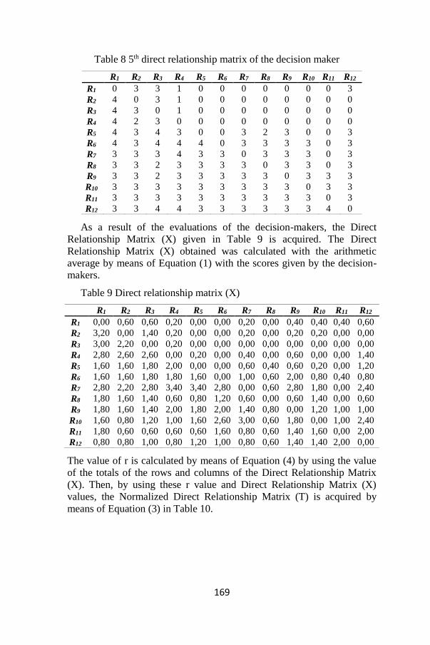
169
Table 8 5th direct relationship matrix of the decision maker
R1 R2 R3 R4 R5 R6 R7 R8 R9 R10 R11 R12
R1 0 3 3 1 0 0 0 0 0 0 0 3
R2 4 0 3 1 0 0 0 0 0 0 0 0
R3 4 3 0 1 0 0 0 0 0 0 0 0
R4 4 2 3 0 0 0 0 0 0 0 0 0
R5 4 3 4 3 0 0 3 2 3 0 0 3
R6 4 3 4 4 4 0 3 3 3 3 0 3
R7 3 3 3 4 3 3 0 3 3 3 0 3
R8 3 3 2 3 3 3 3 0 3 3 0 3
R9 3 3 2 3 3 3 3 3 0 3 3 3
R10 3 3 3 3 3 3 3 3 3 0 3 3
R11 3 3 3 3 3 3 3 3 3 3 0 3
R12 3 3 4 4 3 3 3 3 3 3 4 0
As a result of the evaluations of the decision-makers, the Direct
Relationship Matrix (X) given in Table 9 is acquired. The Direct
Relationship Matrix (X) obtained was calculated with the arithmetic
average by means of Equation (1) with the scores given by the decision-
makers.
Table 9 Direct relationship matrix (X)
R1 R2 R3 R4 R5 R6 R7 R8 R9 R10 R11 R12
R1 0,00 0,60 0,60 0,20 0,00 0,00 0,20 0,00 0,40 0,40 0,40 0,60
R2 3,20 0,00 1,40 0,20 0,00 0,00 0,20 0,00 0,20 0,20 0,00 0,00
R3 3,00 2,20 0,00 0,20 0,00 0,00 0,00 0,00 0,00 0,00 0,00 0,00
R4 2,80 2,60 2,60 0,00 0,20 0,00 0,40 0,00 0,60 0,00 0,00 1,40
R5 1,60 1,60 1,80 2,00 0,00 0,00 0,60 0,40 0,60 0,20 0,00 1,20
R6 1,60 1,60 1,80 1,80 1,60 0,00 1,00 0,60 2,00 0,80 0,40 0,80
R7 2,80 2,20 2,80 3,40 3,40 2,80 0,00 0,60 2,80 1,80 0,00 2,40
R8 1,80 1,60 1,40 0,60 0,80 1,20 0,60 0,00 0,60 1,40 0,00 0,60
R9 1,80 1,60 1,40 2,00 1,80 2,00 1,40 0,80 0,00 1,20 1,00 1,00
R10 1,60 0,80 1,20 1,00 1,60 2,60 3,00 0,60 1,80 0,00 1,00 2,40
R11 1,80 0,60 0,60 0,60 0,60 1,60 0,80 0,60 1,40 1,60 0,00 2,00
R12 0,80 0,80 1,00 0,80 1,20 1,00 0,80 0,60 1,40 1,40 2,00 0,00
The value of r is calculated by means of Equation (4) by using the value
of the totals of the rows and columns of the Direct Relationship Matrix
(X). Then, by using these r value and Direct Relationship Matrix (X)
values, the Normalized Direct Relationship Matrix (T) is acquired by
means of Equation (3) in Table 10.
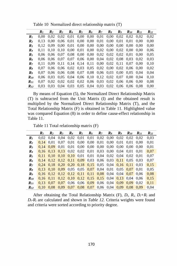
170
Table 10 Normalized direct relationship matrix (T)
R1 R2 R3 R4 R5 R6 R7 R8 R9 R10 R11 R12
R1 0,00 0,02 0,02 0,01 0,00 0,00 0,01 0,00 0,02 0,02 0,02 0,02
R2 0,13 0,00 0,06 0,01 0,00 0,00 0,01 0,00 0,01 0,01 0,00 0,00
R3 0,12 0,09 0,00 0,01 0,00 0,00 0,00 0,00 0,00 0,00 0,00 0,00
R4 0,11 0,10 0,10 0,00 0,01 0,00 0,02 0,00 0,02 0,00 0,00 0,06
R5 0,06 0,06 0,07 0,08 0,00 0,00 0,02 0,02 0,02 0,01 0,00 0,05
R6 0,06 0,06 0,07 0,07 0,06 0,00 0,04 0,02 0,08 0,03 0,02 0,03
R7 0,11 0,09 0,11 0,14 0,14 0,11 0,00 0,02 0,11 0,07 0,00 0,10
R8 0,07 0,06 0,06 0,02 0,03 0,05 0,02 0,00 0,02 0,06 0,00 0,02
R9 0,07 0,06 0,06 0,08 0,07 0,08 0,06 0,03 0,00 0,05 0,04 0,04
R10 0,06 0,03 0,05 0,04 0,06 0,10 0,12 0,02 0,07 0,00 0,04 0,10
R11 0,07 0,02 0,02 0,02 0,02 0,06 0,03 0,02 0,06 0,06 0,00 0,08
R12 0,03 0,03 0,04 0,03 0,05 0,04 0,03 0,02 0,06 0,06 0,08 0,00
By means of Equation (5), the Normalized Direct Relationship Matrix
(T) is subtracted from the Unit Matrix (I) and the obtained result is
multiplied by the Normalized Direct Relationship Matrix (T), and the
Total Relationship Matrix (F) is obtained in Table 11. Highlighted value
was compared Equation (8) in order to define cause-effect relationship in
Table 11.
Table 11 Total relationship matrix (F)
R1 R2 R3 R4 R5 R6 R7 R8 R9 R10 R11 R12
R1 0,02 0,04 0,04 0,02 0,01 0,01 0,02 0,00 0,02 0,02 0,02 0,03
R2 0,14 0,01 0,07 0,01 0,00 0,00 0,01 0,00 0,01 0,01 0,00 0,01
R3 0,14 0,09 0,01 0,01 0,00 0,00 0,00 0,00 0,00 0,00 0,00 0,01
R4 0,16 0,13 0,13 0,02 0,02 0,01 0,03 0,00 0,04 0,01 0,01 0,07
R5 0,11 0,10 0,10 0,10 0,01 0,01 0,04 0,02 0,04 0,02 0,01 0,07
R6 0,14 0,12 0,12 0,11 0,09 0,03 0,06 0,03 0,11 0,05 0,03 0,07
R7 0,24 0,18 0,20 0,20 0,18 0,15 0,05 0,04 0,16 0,11 0,03 0,15
R8 0,13 0,10 0,09 0,05 0,05 0,07 0,04 0,01 0,05 0,07 0,01 0,05
R9 0,16 0,12 0,12 0,12 0,11 0,11 0,08 0,04 0,04 0,07 0,06 0,08
R10 0,16 0,11 0,12 0,10 0,12 0,15 0,15 0,04 0,13 0,04 0,06 0,15
R11 0,13 0,07 0,07 0,06 0,06 0,09 0,06 0,04 0,09 0,09 0,02 0,11
R12 0,10 0,08 0,09 0,07 0,08 0,07 0,06 0,04 0,09 0,08 0,09 0,04
After obtaining the Total Relationship Matrix (F), Di, Ri, Di+Ri and
Di-Ri are calculated and shown in Table 12. Criteria weights were found
and criteria were sorted according to priority degree.
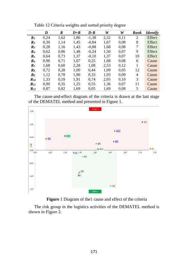
171
Table 12 Criteria weights and sorted priority degree
D R D+R D-R W W Rank Identify
R1 0,24 1,62 1,86 -1,38 2,32 0,11 2 Effect
R2 0,30 1,14 1,45 -0,84 1,67 0,08 8 Effect
R3 0,28 1,16 1,43 -0,88 1,68 0,08 7 Effect
R4 0,62 0,86 1,48 -0,24 1,50 0,07 9 Effect
R5 0,64 0,73 1,37 -0,10 1,37 0,07 10 Effect
R6 0,96 0,71 1,67 0,25 1,68 0,08 6 Cause
R7 1,68 0,60 2,28 1,08 2,53 0,12 1 Cause
R8 0,72 0,28 1,00 0,44 1,09 0,05 12 Cause
R9 1,12 0,78 1,90 0,33 1,93 0,09 4 Cause
R10 1,33 0,59 1,91 0,74 2,05 0,10 3 Cause
R11 0,90 0,35 1,25 0,55 1,36 0,07 11 Cause
R12 0,87 0,82 1,69 0,05 1,69 0,08 5 Cause
The cause-and-effect diagram of the criteria is drawn at the last stage
of the DEMATEL method and presented in Figure 1.
Figure 1 Diagram of the1 cause and effect of the criteria
The risk group in the logistics activities of the DEMATEL method is
shown in Figure 2.
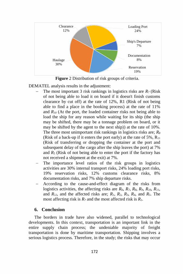
172
Figure 2 Distribution of risk groups of criteria.
DEMATEL analysis results in the adjustment:
The most important 3 risk rankings in logistics risks are R7 (Risk
of not being able to load it on board if it doesn't finish customs
clearance by cut off) at the rate of 12%, R1 (Risk of not being
able to find a place in the booking process) at the rate of 11%
and R10 (At the port, the loaded container risks not being able to
load the ship for any reason while waiting for its ship (the ship
may be shifted, there may be a tonnage problem on board, or it
may be shifted by the agent to the next ship)) at the rate of 10%.
The three most unimportant risk rankings in logistics risks are; R8
(Risk of a back-up if it enters the port early) at the rate of 5%, R11
(Risk of transferring or dropping the container at the port and
subsequent delay of the cargo after the ship leaves the port) at 7%
and R5 (Risk of not being able to enter the port if the factory has
not received a shipment at the exit) at 7%.
The importance level ratios of the risk groups in logistics
activities are 30% internal transport risks, 24% loading port risks,
19% reservation risks, 12% customs clearance risks, 8%
documentation risks, and 7% ship departure risks.
According to the cause-and-effect diagram of the risks from
logistics activities, the affecting risks are R6, R7, R8, R9, R10, R11,
and R12, and the affected risks are; R1, R2, R3, R4, and R5. The
most affecting risk is R7 and the most affected risk is R1.
6. Conclusion
The borders in trade have also widened, parallel to technological
developments. In this context, transportation is an important link in the
entire supply chain process; the undeniable majority of freight
transportation is done by maritime transportation. Shipping involves a
serious logistics process. Therefore, in the study; the risks that may occur
Reservation
19%
Haulage
30%
Clearance
12%Loading Port
24%
Ship's Departure
7%
Documentation
8%

173
during the CIF maritime logistics process, which the seller frequently
chooses in maritime transportation, were determined and the importance
of the risks and the level of impact on each other were determined. In
order to achieve this goal, analyzes were made with the DEMATEL
method, and expert opinions were used to determine the risks and their
importance. While there are many studies on risk management in the
literature, this study contributed to the application area of the literature.
The weights of the risks considered were listed between 5% and 12% in
the study. The highest risk was found to be R7 (Risk of not being able to
load it on board if it doesn't finish customs clearance by cut off) with
12%. The least important risk in logistics risks; it is R8 (Risk of a back-up
if it enters the port early) with a rate of 5%. Ratios of importance level of
risk groups in logistics activities; internal transport risks have a share of
30%; ship departure risks have the lowest share with 7%. According to
the cause-and-effect diagram of the risks arising from logistics activities;
the risk most impacting is R7 (Risk of not being able to load it on board if
it doesn't finish customs clearance by cut off) and the risk most impacted
is R1 (Risk of not being able to find a place in the booking process).
It was ensured that the risks in the operation processes of the logistics
enterprises were determined, their importance levels were listed and their
relations with each other were evaluated with the proposed model. In
future studies, similar approaches can be applied to different application
areas, other operations or other processes of logistics enterprises.
References
Aksakal, E., and Dağdeviren, M., ANP ve DEMATEL Yöntemleri ile
Personel Seçimi Problemine Bütünleşik Bir Yaklaşım, Gazi
Üniversitesi Mühendislik Mimarlık Fakültesi Dergisi, Cilt. 25, No. 4,
(2010), ss. 905-913.
Chiu, Y. J., Chen, H. C., Tzeng, G. H., and Shyu, J. Z., Marketing
strategy based on customer behaviour for the LCD-TV, International
Journal and Decision Making, Vol. 7 No. 2/3 (2006), pp. 143–165.
Du, S., Li, H., and Sun, B., Hybrid Kano-fuzzy-DEMATEL model based
risk factor evaluation and ranking of cross-border e-commerce SMEs
with customer requirement, Journal of Intelligent & Fuzzy
Systems, Vol. 37 No.6 (2019), pp. 8299-8315.
Faghih-Roohi S., Akcay A., Zhang Y., Shekarian E., and Jong E., A
group risk assessment approach for the selection of pharmaceutical
product shipping lanes, International Journal Production Economics,
Vol. 229 (November 2020) 107774.

174
Freydman, O., The role of risk management of the logistic processes in
economic development of the region, Studies of the Industrial
Geography Commission of the Polish Geographical Society, No. 18
(2011), pp. 139-147.
Ganguly K. K., and Kumar G., Supply chain risk assessment: A fuzzy
AHP approach, Operations and Supply Chain Management, Vol. 12
No. 1 (2019), pp. 1 – 13.
Govindan K. and Chaudhuri A., Interrelationships of risks faced by third
party logistics service providers: A DEMATEL based approach,
Transportation Research Part E Vol. 90 (2016), pp. 177–195.
Grant, D. B., and Elliott, M., A proposed interdisciplinary framework for
the environmental management of water and air-borne emissions in
maritime logistics, Ocean & coastal management, Vol. 163 (2018), pp.
162-172.
Habegger B., Risk analysis and management in a dynamic risk landscape,
International Handbook on Risk Analysis and Management
Professional Experiences Edited by Beat Habegger, (2008), pp. 13-32,
ISBN 3-905696-18-5.
Huang, C.Y., Shyu, J.Z.,and Tzeng, G.H., Reconfiguring the innovation
policy portfolios for Taiwan’s SIP Mall industry, Technovation, Vol.
27 No. 12 (2007), pp. 744–765.
ICC., Incoterms 2020, by The International Chamber of Commerce,
(2019), ISBN: 978-92-842-0511-0.
ISO, BS ISO 31000:2018 BSI standards publication risk management —
Guidelines, Second edition (2018) Reference number ISO
31000:2018(E)
Kalogeraki E.M., Papastergiou S., Mouratidis H., and Polemi N. A.,
Novel risk assessment methodology for SCADA maritime logistics
environments, Applied Sciences (2018), 8, 1477.
Karaoğlan S., DEMATEL ve VIKOR Yöntemleriyle Dış Kaynak Seçimi:
Otel İşletmesi Örneği. Akademik Bakış Uluslararası Hakemli Sosyal
Bilimler Dergisi, Sayı.55 (Mayıs Haziran 2016), ss. 9-24.
Laudares A.C., Ricco M.F.F., and Santos R.A.S., When does it end?
Monte Carlo simulation applied to risk management indefense
logistics’ procurement processes, Brazilian Journal of Operations ve
Production Management, Vol.16 No. 1 (2019), pp. 149-156.
Li, R. J., Fuzzy method in group decision making, Computers and
Mathematics with Applications, Vol. 38 No.1 (1999), pp. 91–101.
Liou, J. H., Yen, L., and Tzeng, G. H., Building an effective safety
management system for airlines, Journal of Air Transport
Management, Vol.14, No.1 (2008), pp. 20-26.
175
Liou, J.H., Tzeng, H.G., and Chang, H.C., Airline safety measurement
using a Novel Hybrid Model, Journal of Air Transport Management,
Vol. 13 No. 4 (2007), pp. 243-249.
Liu, J., Zhou, H., and Sun, H., A three-dimensional risk management
model of port logistics for hazardous goods, Maritime Policy &
Management, Vol. 46, No.6 (2019), pp. 715-734.
Mokhtari, K., and Ren, J., A risk management methodology for maritime
logistics and supply chain applications, Ocean Systems
Engineering, Vol. 4 No. 2 (2014), pp. 137-150.
Nam, H. S., and Song, D. W., Defining maritime logistics hub and its
implication for container port, Maritime Policy & Management, Vol.
38 No. 3 (2011), pp. 269-292.
Nguyen S., A risk assessment model with systematical uncertainty
treatment for container shipping operations, Maritime Policy &
Management, Vol. 47 No. 6 (2020), pp. 778-796.
Nikolov, B., and Tcholakova, V., Aspects of risk management in logistics
activities of enterprises, application of fault tree analysis
(fta). Innovations, Vol. 3 No. 2 (2015), pp. 34-38.
Papastergiou, S., and Polemi, D., Securing maritime logistics and supply
chain: the medusa and MITIGATE approaches, Maritime Interdiction
Operation Journal, No.14 (2017), pp. 42-48.
Radhika, D., The role of knowledge management as an innovative
strategy in maritime logistics management, International Journal of
Humanities Social Sciences and Education, Vol.1 No. 9 (2014), pp.
52-57.
Rahman M. S., Khan F., Shaikh A., Ahmed S. and Imtiaz S., A
conditional dependence-based marine logistics support risk model,
Reliability Engineering & System Safety Vol. 193, (January 2020),
106623.
Roh S., Tam J., Lee S.W., and Seo Y. J., Risk assessment of maritime
supply chain security in ports and waterways, International Journal of
Supply Chain Management, Vol. 7, No. 6 (2018),pp. 300-307.
Seredyuk V., Incoterms in practice: hidden risks case study Glaston.
Bachelor’s thesis,Tampere University of Applied Sciences Degree
Programme in International Business School of Business and
Services, (Autumn 2017).
Seyed-Hosseini, S. M., Safaei, N., and Asgharpour, M. J., (2006).
Reprioritization of failures in a system failure mode and effects
analysis by decision making trial and evaluation laboratory technique
eliability. Engineering and System Safety, Vol. 91 No. 8 (2006), pp.
872–881.
176
Tzeng, G. H., and Huang, J. J., Multiple Attribute Decision Making
Methods and Applications. Boca Raton (USA): CRC Press, (2011)
159.
Tzeng, G. H., Chiang, C. H., and Li, C. W., Evaluating intertwined
effects in e-learning programs: A novel hybrid MCDM model based
on factor analysis and DEMATEL, Expert Systems with Applications,
Vol.32 No. 4 (2007), pp. 1028–1044.
UNCTAD, Review of Maritime Transport 2020, (2020), New York:
United Nations Publications. ISBN 978-92-1-112993-9.
Vilkoa J., Ritalaa P., and Hallikasa J., Risk management abilities in
multimodal maritime supply chains: Visibility and control
perspectives. Accident Analysis and Prevention, Vol. 123 (2019), pp.
469–481.
Wu, W. W., and Lee, Y.T., Developing global managers’ competencies
using the fuzzy DEMATEL method, Expert Systems with
Applications, Vol. 32, No. 20 (2007), pp. 499-507.
Yin E., Chen Z., and Xiao Y., Risk perception affecting the performance
of shipping companies: the moderating effect of China and Korea,
Maritime Policy & Management, Vol. 46 No. 3 (2019), pp. 295-308.
Zimon D., and Madzík P., Standardized management systems and risk
management in the supply chain, International Journal of Quality and
Reliability Management Vol. 37 No. 2 (2020), pp. 305-327.