PRACTICE OF A

CARL& A. SMITB. Co

SELECTED TABLES AND FIGURES

TYPICAL RESPONSESCommon input s ignals 1 3Stable and unstable responses 3 4

First-order step response 42First-order ramp response 44

First-order sinusoidal response 4 5Lead-lag step responseLead-lag ramp response 48Second-order step response

TRANSFORMS transforms 1 5

z-transforms and modified z-transforms 607

TUNING FORMULASOn-line quarter decay ratio 306Open-loop quarter decay ratio 320Minimum error integral for disturbance 324Minimum error integral for set point 325Controller synthesis (IMC) rules 345Computer PID control algorithms 666Dead t ime compensation algorithms 675

INSTRUMENTATIONISA standard instrumentation symbols and

labelsControl valve inherent characteristicsControl valve installed characteristicsFlow sensors and their characteristicsTemperature sensors and their

characteristicsClassification of filled-system thermometersThermocouple voltage versus temperatureValve capacity (Cv) coefficients

699-706

211217

724-725736-737

739740

754-755

BLOCK DIAGRAMSRules 98

Feedback loop 254Unity feedback loop 257Temperature control loop 261

Flow control loop 268Pressure control loop 281Level control loop 333Multivariable (2 X 2) control loop 565Decoupled multivariable (2 X 2) system 566Sampled data control loop 630Smith predictor 679Internal Model Control (IMC) 680Dynamic Matrix Control (DMC) 689

Principles and Practice ofAutomatic Process Control

Second Edition

Carlos A. Smith, Ph.D., P.E.University of South Florida

Armando B. Corripio, Ph.D., P.E.Louisiana State University

John Wiley Sons, Inc.New York � Chichester � Weinheim � Brisbane � Singapore � Toronto

This work is dedicated with all our love to The our God,for all his daily blessings made this book possible

The Smiths:Cristina, A. Jr., Tim, Cristina M., and Sophia C. Livingston,and Mrs. Rene M. Smith,

my four grandsons:Nicholas, Robert, Garrett and David

and to our dearest homeland, Cuba

Preface

This edition is a major revision and expansion to the first edition. Several new subjectshave been added, notably the z-transform analysis and discrete controllers, and severalother subjects have been reorganized and expanded. The objective of the book, however,remains the same as in the first edition, “to present the practice of automatic processcontrol along with the fundamental principles of control theory.” A significant numberof applications resulting from our practice as part-time consultants have also been addedto this edition.

Twelve years have passed since the first edition was published, and even though theprinciples are still very much the same, the “tools” to implement the controls strategieshave certainly advanced. The use of computer-based instrumentation and control sys-tems is the norm.

Chapters 1 and 2 present the definitions of terms and mathematical tools used inprocess control. In this edition Chapter 2 stresses the determination of the quantitativecharacteristics of the dynamic response, settling time, frequency of oscillation, anddamping ratio, and de-emphasizes the exact determination of the analytical response.In this way the students can analyze the response of a dynamic system without havingto carry out the time-consuming evaluation of the coefficients in the partial fractionexpansion. Typical responses of first-, second-, and higher-order systems are now pre-sented in Chapter 2.

The derivation of process dynamic models from basic principles is the subject ofChapters 3 and 4. As compared to the first edition, the discussion of process modellinghas been expanded. The discussion, meaning, and significance of process nonlinearitieshas been expanded as well. Several numerical examples are presented to aid in theunderstanding of this important process characteristic. Chapter 4 concludes with a pre-sentation of integrating, inverse-response, and open-loop unstable processes.

Chapter 5 presents the design and characteristics of the basic components of a controlsystem: sensors and transmitters, control valves, and feedback controllers. The presen-tation of control valves and feedback controllers has been expanded. Chapter 5 shouldbe studied together with Appendix C where practical operating principles of somecommon sensors, transmitters, and control valves are presented.

The design and tuning of feedback controllers are the subjects of Chapters 6 and 7.Chapter 6 presents the analysis of the stability of feedback control loops. In this editionwe stress the direct substitution method for determining both the ultimate gain andperiod of the loop. Routh’s test is deemphasized, but still presented in a separate section.In keeping with the spirit of Chapter 2, the examples and problems deal with the de-termination of the characteristics of the response of the closed loop, not with the exactanalytical response of the loop. Chapter 7 keeps the same tried-and-true tuning methodsfrom the first edition. A new section on tuning controllers for integrating processes,and a discussion of the Internal Model Control (IMC) tuning rules, have been added.

Chapter 8 presents the root locus technique, and Chapter 9 presents the frequencyresponse techniques. These techniques are principally used to study the stability ofcontrol systems.

V

vi Preface

The additional control techniques that supplement and enhance feedback control havebeen distributed among Chapters 10 through 13 to facilitate the selection of their cov-erage in university courses. Cascade control is presented first, in Chapter 10, becauseit is so commonly a part of the other schemes. Several examples are presented to helpunderstanding of this important and common control technique.

Chapter 11 presents different computing algorithms sometimes used to implementcontrol schemes. A method to scale these algorithms, when necessary, is presented. Thechapter also presents the techniques of override, or constraint, control, and selectivecontrol. Examples are used to explain the meaning and justification of them.

Chapter 12 presents and discusses in detail the techniques of ratio and feedforwardcontrol. Industrial examples are also presented. A significant number of new problemshave been added.

Multivariable control and loop interaction are the subjects of Chapter 13. The cal-culation and interpretation of the relative gain matrix (RGM) and the design ofcouplers, are kept from the first edition. Several examples have been added, and thematerial has been reorganized to keep all the dynamic topics in one section.

Finally Chapters 14 and 15 present the tools for the design and analysis of data (computer) control systems. Chapter 14 presents the z-transform and its use toanalyze sampled-data control systems, while Chapter 15 presents the design of basicalgorithms for computer control and the tuning of sampled-data feedback controllers.The chapter includes sections on the design and tuning of dead-time compensationalgorithms and model-reference control algorithms. Two examples of Dynamic MatrixControl (DMC) are also included.

As in the first edition, Appendix A presents some symbols, labels, and other notationscommonly used in instrumentation and control diagrams. We have adopted throughoutthe book the ISA symbols for conceptual diagrams which eliminate the need to differ-entiate between pneumatic, electronic, or computer implementation of the various con-trol schemes. In keeping with this spirit, we express all instrument signals in percentof range rather than in or psig. Appendix B presents several processes to providethe student/reader an opportunity to design control systems from scratch.

During this edition we have been very fortunate to have received the help and en-couragement of several wonderful individuals. The encouragement of our students,especially Daniel Palomares, Denise Farmer, Carl Thomas, Gene Daniel, Samuelbles, Dan Logue, and Steve Hunter, will never be forgotten. Thanks are also due to Dr.Russell Rhinehart of Texas Tech University who read several chapters when they werein the initial stages. His comments were very helpful and resulted in a better book.Professors Ray Wagonner, of Missouri and G. David Shilling, of Rhode Island,gave us invaluable suggestions on how to improve the first edition. To both of themwe are grateful. We are also grateful to Michael R. Benning of Exxon Chemical Amer-icas who volunteered to review the manuscript and offered many useful suggestionsfrom his industrial background.

In the preface to the first edition we said that “To serve as agents in the training anddevelopment of young minds is certainly a most rewarding profession.” This is still ourconviction and we feel blessed to be able to do so. It is with this desire that we havewritten this edition.

Tampa, Florida, 1997

Baton Rouge, Louisiana, 1997

Contents

Chapter 1 Introductionl - l1-21-31-41-5

1-61-7

A Process Control System 1Important Terms and the Objective of Automatic Process ControlRegulatory and Servo Control 4Transmission Signals, Control Systems, and Other Terms 5Control Strategies 61-5.1 Feedback Control 61-5.2 Feedforward Control 7Background Needed for Process Control 9S u m m a r y 9P r o b l e m s 9

3

1

Chapter 2 Mathematical Tools for Control Systems Analysis2-1 The Transform 11

1.1 Definition of Transform 122-1.2 Properties of the Transform 14

2-2 Solution of Differential Equations Using the Transform 212-2.1 Transform Solution Procedure 212-2.2 Inversion by Partial Fractions Expansion 232-2.3 Handling Time Delays 27

2-3 Characterization of Process Response 302-3.1 Deviation Variables 3 12-3.2 Output Response 322 -3 .3 S t ab i l i t y 39

2-4 Response of First-Order Systems 392-4.1 Step Response 412-4.2 Ramp Response 432-4.3 Sinusoidal Response 432-4.4 Response with Time Delay 452-4.5 Response of a Lead-Lag Unit 46

2-5 Response of Second-Order Systems 482-5.1 Overdamped Responses 502-5.2 Underdamped Responses 532-5.3 Higher-Order Responses 57

2-6 Linearization 592-6.1 Linearization of Functions of One Variable 602-6.2 Linearization of Functions of Two or More Variables 622-6.3 Linearization of Differential Equations 65

2-7 Review of Complex-Number Algebra 682-7.1 Complex Numbers 682-7.2 Operations with Complex Numbers 70

11

vi i

viii Contents

2-8 S u m m a r y 7 4Prob lems 74

Chapter 3 First-Order Dynamic Systems 803-13-23-33-4

3-53-6

3-73-83-9

Processes and the Importance of Process CharacteristicsThermal Process Example 82Dead Time 92Transfer Functions and Block Diagrams 953-4.1 Transfer Functions 953-4.2 Block Diagrams 96Gas Process Example 104Chemical Reactors 1093-6.1 Introductory Remarks 1093-6.2 Chemical Reactor Example 111Effects of Process Nonlinearities 114Additional Comments 117Summary 119Problems 120

81

Chapter 4 Higher-Order Dynamic Systems4-1 Noninteracting Systems 135

1.1 Noninteracting Level Process 135 1.2 Thermal Tanks in Series 142

4-2 Interacting Systems 1454-2.1 Interacting Level Process 1454-2.2 Thermal Tanks with Recycle 1514-2.3 Nonisothermal Chemical Reactor 154

4-3 Response of Higher-Order Systems 1644-4 Other Types of Process Responses 167

4-4.1 Integrating Processes: Level Process 1684-4.2 Open-Loop Unstable Process: Chemical Reactor 1724-4.3 Inverse Response Processes: Chemical Reactor 179

4-5 Summary 1814-6 Overview of Chapters 3 and 4 182

Prob lems 183

Chapter 5 Basic Components of Control Systems5-1 Sensors and Transmitters 1975-2 Control Valves 200

5-2.1 The Control Valve Actuator 2005-2.2 Control Valve Capacity and Sizing 2025-2.3 Control Valve Characteristics 2105-2.4 Control Valve Gain and Transfer Function 2165-2.5 Control Valve Summary 222

5-3 Feedback Controllers 2225-3.1 Actions of Controllers 223

1 3 5

1 9 7

Contents ix

5-4

5-3.2 Types of Feedback Controllers 2255-3.3 Modifications to the PID Controller and Additional Comments5-3.4 Reset Windup and Its Prevention 2415-3.5 Feedback Controller Summary 244Summary 244Prob lems 245

238

Chapter 6 Design of Single-Loop Feedback Control Systems 2526-1 The Feedback Control Loop 252

1.1 Closed-Loop Transfer Function 2556-1.2 Characteristic Equation of the Loop 2636-1.3 Steady-State Closed-Loop Gains 270

6-2 Stability of the Control Loop 2746-2.1 Criterion of Stability 2746-2.2 Direct Substitution Method 2756-2.3 Effect of Loop Parameters on the Ultimate Gain and Period 2836-2.4 Effect of Dead Time 2856-2.5 Routh’s Test 287

6-3 Summary 290Prob lems 290

Chapter 7 Tuning of Feedback Controllers 3037-17-2

7-3

7-4

7-5

7-6

Quarter Decay Ratio Response by Ultimate Gain 304Open-Loop Process Characterization 3087-2.1 Process Step Testing 3107-2.2 Tuning for Quarter Decay Ratio Response 3197-2.3 Tuning for Minimum Error Integral Criteria 3217-2.4 Tuning Sampled-Data Controllers 3297-2.5 Summary of Controller Tuning 330Tuning Controllers for Integrating Processes 3317-3.1 Model of Liquid Level Control System 3317-3.2 Proportional Level Controller 3347-3.3 Averaging Level Control 3367-3.4 Summary 337Synthesis of Feedback Controllers 3377-4.1 Development of the Controller Synthesis Formula 3377-4.2 Specification of the Closed-Loop Response 3387-4.3 Controller Modes and Tuning Parameters 3397-4.4 Summary of Controller Synthesis Results 3447-4.5 Tuning Rules by Internal Model Control (IMC) 350Tips for Feedback Controller Tuning 3517-5.1 Estimating the Integral and Derivative Times 3527-5.2 Adjusting the Proportional Gain 354Summary 354Problems 355

x Contents

Chapter 8 Root Locus 3688-18-28-38-4

Some Definitions 368Analysis of Feedback Control Systems by Root LocusRules for Plotting Root Locus Diagrams 375Summary 385Prob lems 386

370

Chapter 9 Frequency Response Techniques9-1 Frequency Response 389

1.1 Experimental Determination of Frequency Response 3899-1 .2 Bode P lo t s 398

9-2 Frequency Response Stability Criterion 4079-3 Polar Plots 4199-4 Nichols Plots 4279-5 Pulse Testing 427

9-5.1 Performing the Pulse Test 4289-5.2 Derivation of the Working Equation 4299-5.3 Numerical Evaluation of the Fourier Transform Integral 431

9-6 Summary 434Prob lems 434

Chapter 10 Cascade Control10-1 A Process Example 43910-2 Stability Considerations 44210-3 Implementation and Tuning of Controllers 445

10-3.1 Two-Level Cascade Systems 44610-3.2 Three-Level Cascade Systems 449

10-4 Other Process Examples 45010-5 Further Comments 452

Summary 453Prob lems 454

Chapter 11 Override and Selective Control11-1 Computing Algorithms 460

1 1 1.1 Scaling Computing Algorithms 4641 l-l.2 Physical Significance of Signals 469

11-2 Override, or Constraint, Control 47011-3 Selective Control 47511-4 Summary 479

Prob lems 479

Chapter 12 Ratio and Feedforward Control12-1 Ratio Control 48712-2 Feedforward Control 494

389

4 3 9

460

4 8 7

Chapter 13 Multivariable Process Control 5 4 513-1 Loop Interaction 54513-2 Pairing Controlled and Manipulated Variables 550

13-2.1 Calculating the Relative Gains for a 2 X 2 System 55413-2.2 Calculating the Relative Gains for an X System 561

13-3 Decoupling of Interacting Loops 56413-3.1 Decoupler Design from Block Diagrams 56513-3.2 Decoupler Design for X Systems 57313-3.3 Decoupler Design from Basic Principles 577

13-4 Multivariable Control vs. Optimization 57913-5 Dynamic Analysis of Multivariable Systems 580

13-5.1 Signal Flow Graphs (SFG) 58013-5.2 Dynamic Analysis of a 2 X 2 System 58513-5.3 Controller Tuning for Interacting Systems 590

13-6 Summary 592Prob lems 592

Contents xi

12-2.1 The Feedforward Concept 49412-2.2 Block Diagram Design of Linear Feedforward Controllers 49612-2.3 Lead/Lag Term 50512-2.4 Back to the Previous Example 50712-2.5 Design of Nonlinear Feedforward Controllers from Basic Process

Pr inc ip l e s 51112-2.6 Some Closing Comments and Outline of Feedforward Controller

D e s i g n 5 1 512-2.7 Three Other Examples 518

12-3 Summary 526Prob lems 527

Chapter 14 Mathematical Tools for Computer Control Systems 5 9 914-114-2

14-3

14-4

14-5

Computer Process Control 600The z-Transform 60114-2.1 Definition of the z-Transform 60114-2.2 Relationship to the Transform 60514-2.3 Properties of the 60914-2.4 Calculation of the Inverse z-Transform 613Pulse Transfer Functions 61614-3.1 Development of the Pulse Transfer Function 61614-3.2 Steady-State Gain of a Pulse Transfer Function 62014-3.3 Pulse Transfer Functions of Continuous Systems 62114-3.4 Transfer Functions of Discrete Blocks 62514-3.5 Simulation of Continuous Systems with Discrete Blocks 627Sampled-Data Feedback Control Systems 62914-4.1 Closed-Loop Transfer Function 63014-4.2 Stability of Sampled-Data Control Systems 632Modified z-Transform 63814-5.1 Definition and Properties of the Modified z-Transform 639

xii Contents

14-6

14-5.2 Inverse of the Modified z-Transform 64214-5.3 Transfer Functions for Systems with Transportation LagSummary 645Prob lems 645

643

Chapter 15 Design of Computer Control Systems15-1 Development of Control Algorithms 650

1.1 Exponential Filter 651 1.2 Lead-Lag Algorithm 653 1.3 Feedback (PID) Control Algorithms 655

15-2 Tuning of Feedback Control Algorithms 66215-2.1 Development of the Tuning Formulas 66215-2.2 Selection of the Sample Time 672

15-3 Feedback Algorithms with Dead-Time Compensation 67415-3.1 The Dahlin Algorithm 67415-3.2 The Smith Predictor 67715-3.3 Algorithm Design by Internal Model Control 68015-3.4 Selection of the Adjustable Parameter 685

15-4 Automatic Controller Tuning 68715-5 Model-Reference Control 68815-6 Summary 695

Prob lems 696

Appendix A Instrumentation Symbols and Labels

Appendix B Case Studies 7 0 7Case 1: Ammonium Nitrate Prilling Plant Control System 707Case 2: Natural Gas Dehydration Control System 709Case 3: Sodium Hypochlorite Bleach Preparation Control System 710Case 4: Control Systems in the Sugar Refining Process 711Case 5: CO, Removal from Synthesis Gas 712Case 6: Sulfuric Acid Process 716Case 7: Fatty Acid Process 717

Appendix C Sensors, Transmitters, and Control ValvesC-l Pressure Sensors 721c-2 Flow Sensors 723c-3 Level Sensors 733c-4 Temperature Sensors 734c-5 Composition Sensors 742C-6 Transmitters 743

C-6.1 Pneumatic Transmitter 743C-6.2 Electronic Transmitter 745

C-7 Types of Control Valves 745C-7.1 Reciprocating Stem 745C-7.2 Rotating Stem 750

650

699

721

Contents xiii

c-9

Control Valve Actuators 750Pneumatically Operated Diaphragm Actuators 750

C-8.2 Piston Actuators 750C-8.3 Electrohydraulic and Electromechanical Actuators 751C-8.4 Manual-Handwheel Actuators 751Control Valve Accessories 752C-9.1 Positioners 752C-9.2 Boosters 753C-9.3 Limit Switches 753Control Valves-Additional Considerations 753C- 10.1 Viscosity Corrections 753C-lo.2 Flashing and Cavitation 756Summary 760

Index 7 6 3

Chapter 1

Introduction

The purpose of this chapter is to present the need for automatic process control and tomotivate you, the reader, to study it. Automatic process control is concerned withmaintaining process variables, temperatures, pressures, flows, compositions, and thelike at some desired operating value. As we shall see, processes are dynamic in nature.Changes are always occurring, and if appropriate actions are not taken in response, thenthe important process variables-those related to safety, product quality, and produc-tion rates-will not achieve design conditions.

This chapter also introduces two control systems, takes a look at some of their com-ponents, and defines some terms used in the field of process control. Finally, the back-ground needed for the study of process control is discussed.

In writing this book, we have been constantly aware that to be successful, the engineermust be able to apply the principles learned. Consequently, the book covers the prin-ciples that underlie the successful practice of automatic process control. The book isfull of actual cases drawn from our years of industrial experience as full-time practi-tioners or part-time consultants. We sincerely hope that you get excited about studyingautomatic process control. It is a very dynamic, challenging, and rewarding area ofprocess engineering.

l-l A PROCESS CONTROL SYSTEM

To illustrate process control, let us consider a heat exchanger in which a process streamis heated by condensing steam; the process is sketched in Fig. 1-1.1. The purpose ofthis unit is to heat the process fluid from some inlet temperature up to a certaindesired outlet temperature T(t). The energy gained by the process fluid is provided bythe latent heat of condensation of the steam.

In this process there are many variables that can change, causing the outlet temper-ature to deviate from its desired value. If this happens, then some action must be takento correct the deviation. The objective is to maintain the outlet process temperature atits desired value.

One way to accomplish this objective is by measuring the temperature T(t), compar-ing it to the desired value, and, on the basis of this comparison, deciding what to do tocorrect any deviation. The steam valve can be manipulated to correct the deviation.That is, if the temperature is above its desired value, then the steam valve can be

1

2 Chapter 1 Introduction

C o n d e n s a t ereturn

Figure 1-1.1 Heat exchanger.

throttled back to cut the steam flow (energy) to the heat exchanger. If the temperatureis below the desired value, then the steam valve can be opened more to increase thesteam flow to the exchanger. All of this can be done manually by the operator, and theprocedure is fairly straightforward. However, there are several problems with suchmanual control. First, the job requires that the operator look at the temperature fre-quently to take corrective action whenever it deviates from the desired value. Second,different operators make different decisions about how to move the steam valve, andthis results in a less than perfectly consistent operation. Third, because in most processplants there are hundreds of variables that must be maintained at some desired value,manual correction requires a large number of operators. As a result of these problems,we would like to accomplish this control automatically. That is, we would like to havesystems that control the variables without requiring intervention from the operator. Thisis what is meant by automatic process control.

To achieve automatic process control, a control system must be designed and imple-mented. A possible control system for our heat exchanger is shown in Fig. 1-1.2.

Steam

returnFigure l-l.2 Heat exchanger control system.

1-2 Important Terms and the Objective of Automatic Process Control 3

pendix A presents the symbols and identifications for different devices.) The first thingto do is measure the outlet temperature of the process stream. This is done by a sensor(thermocouple, resistance temperature device, filled system thermometer, thermistor, orthe like). Usually this sensor is physically connected to a transmitter, which takes theoutput from the sensor and converts it to a signal strong enough to be transmitted to acontroller. The controller then receives the signal, which is related to the temperature,and compares it with the desired value. Depending on the result of this comparison, thecontroller decides what to do to maintain the temperature at the desired value. On thebasis of this decision, the controller sends a signal to the final control element, whichin turn manipulates the steam flow. This type of control strategy is known as feedbackcontrol.

Thus the three basic components of all control systems are

1. Sensor/transmitter Also often called the primary and secondary elements.2. Controller The “brain” of the control system.3. Final control element Often a control valve but not always. Other common final

control elements are variable-speed pumps, conveyors, and electric motors.

These components perform the three basic operations that must be present in everycontrol system. These operations are

1. Measurement(M) Measuring the variable to be controlled is usually done by thecombination of sensor and transmitter. In some systems, the signal from the sensorcan be fed directly to the controller, so there is no need for the transmitter.

2. Decision On the basis of the measurement, the controller decides what to doto maintain the variable at its desired value.

3. Action (A) As a result of the controller’s decision, the system must then take anaction. This is usually accomplished by the final control element.

These three operations, M, D, and A, are always present in every type of controlsystem, and it is imperative that they be in a loop. That is, on the basis of the mea-surement a decision is made, and on the basis of this decision an action is taken. Theaction taken must come back and affect the measurement; otherwise, it is a majorin the design, and control will not be achieved. When the action taken does not affectthe measurement, an open-loop condition exists and control will not be achieved. Thedecision making in some systems is rather simple, whereas in others it is more complex;we will look at many systems in this book.

1-2 IMPORTANT TERMS AND THE OBJECTIVE OF AUTOMATICPROCESS CONTROL

At this time it is necessary to define some terms used in the field of automatic processcontrol. The controlled variable is the variable that must be maintained, or controlled,at some desired value. In our example of the heat exchanger, the process outlet tem-perature, T(t), is the controlled variable. Sometimes the term process variable is alsoused to refer to the controlled variable. The set point (SP) is the desired value of thecontrolled variable. Thus the job of a control system is to maintain the controlledvariable at its set point. The manipulated variable is the variable used to maintain thecontrolled variable at its set point. In the example, the steam valve position is the

4 Chapter 1 Introduction

manipulated variable. Finally, any variable that causes the controlled variable to deviatefrom the set point is known as a disturbance or upset. In most processes there are anumber of different disturbances. In the heat exchanger shown in Fig. 1-1.2, possibledisturbances include the inlet process temperature, the process flow, the en-ergy content of the steam, ambient conditions, process fluid composition, and fouling.It is important to understand that disturbances are always occurring in processes. Steadystate is not the rule, and transient conditions are very common. It is because of thesedisturbances that automatic process control is needed. If there were no disturbances,then design operating conditions would prevail and there would be no need to “monitor”the process continuously.

The following additional terms are also important. Manual control is the conditionin which the controller is disconnected from the process. That is, the controller is notdeciding how to maintain the controlled variable at set point. It is up to the operator tomanipulate the signal to the final control element to maintain the controlled variable atset point. Closed-loop control is the condition in which the controller is connected tothe process, comparing the set point to the controlled variable and determining andtaking corrective action.

Now that we have defined these terms, we can express the objective of an automaticprocess control system meaningfully: The objective of an automatic process controlsystem is to adjust the manipulated variable to maintain the controlled variable at itsset point in spite of disturbances.

Control is important for many reasons. Those that follow are not the only ones, butwe feel they are the most important. They are based on our industrial experience, andwe would like to pass them on. Control is important to

1. Prevent injury to plant personnel, protect the environment by preventing emissionsand minimizing waste, and prevent damage to the process equipment. SAFETYmust always be in everyone’s mind; it is the single most important consider-ation.

2. Maintain product quality (composition, purity, color, and the like) on a continuousbasis and with minimum cost.

3. Maintain plant production rate at minimum cost.

Thus process plants are automated to provide a safe environment and at the same maintain desired product quality, high plant throughput, and reduced demand on

human labor.

1-3 REGULATORY AND SERVO CONTROL

In some processes, the controlled variable deviates from set point because of distur-bances. Systems designed to compensate for these disturbances exert regulatorycontrol. In some other instances, the most important disturbance is the set point itself.That is, the set point may be changed as a function of time (typical of this is a batchreactor where the temperature must follow a desired profile), and therefore the con-trolled variable must follow the set point. Systems designed for this purpose exert servocontrol.

Regulatory control is much more common than servo control in the process

1-4 Transmission Signals, Control Systems, and Other Terms

tries. However, the same basic approach is used in designing both. Thus the principlesin this book apply to both cases.

1-4 TRANSMISSION SIGNALS, CONTROL SYSTEMS, AND OTHERTERMS

Three principal types of signals are used in the process industries. The pneumatic signal,or air pressure, normally ranges between 3 and 15 psig. The usual representation forpneumatic signals in process and instrumentation diagrams is The electrical signal normally ranges between 4 and 20 Less often, a range of to 50 1 to 5 V, or 0 to 10 V is used. The usual representation for this signal in

is a series of dashed lines such as The third type of signal is the digital,or discrete, signal (zeros and ones). In this book we will show such signals as (see Fig. which is the representation proposed by the Instrument Society ofAmerica (ISA) when a control concept is shown without concern for specific hardware.The reader is encouraged to review Appendix A, where different symbols and labelsare presented. Most times we will refer to signals as percentages instead of using psigor That is, 0%- 100% is equivalent to 3 to 15 psig or 4 to 20

It will help in understanding control systems to realize that signals are used by de-vices-transmitters, controllers, final control elements, and the like-to communicate.That is, signals are used to convey information. The signal from the transmitter to thecontroller is used by the transmitter to inform the controller of the value of the controlledvariable. This signal is not the measurement in engineering units but rather is apsig, volt, or any other signal that is proportional to the measurement. The relationshipto the measurement depends on the calibration of the sensor/transmitter. The controlleruses its output signal to tell the final control element what to do: how much to open ifit is a valve, how fast to run if it is a variable-speed pump, and so on.

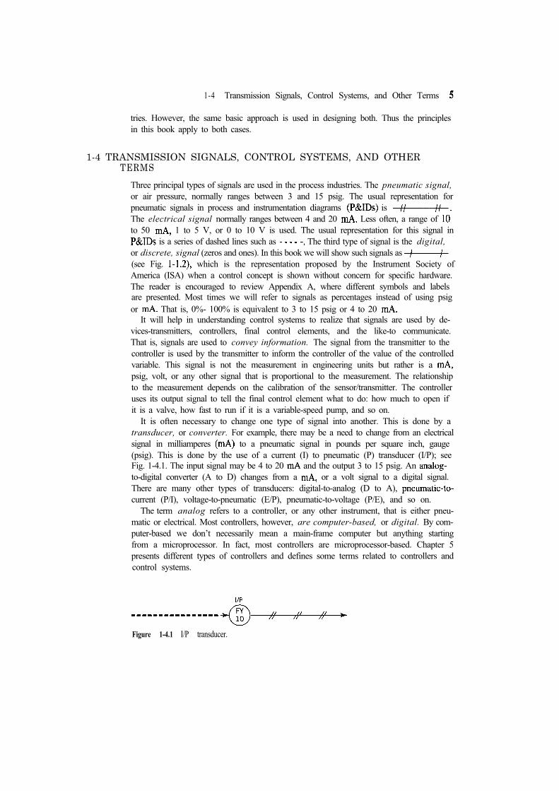
It is often necessary to change one type of signal into another. This is done by atransducer, or converter. For example, there may be a need to change from an electricalsignal in milliamperes to a pneumatic signal in pounds per square inch, gauge(psig). This is done by the use of a current (I) to pneumatic (P) transducer (I/P); seeFig. 1-4.1. The input signal may be 4 to 20 and the output 3 to 15 psig. An to-digital converter (A to D) changes from a or a volt signal to a digital signal.There are many other types of transducers: digital-to-analog (D to A),current (P/I), voltage-to-pneumatic (E/P), pneumatic-to-voltage (P/E), and so on.

The term analog refers to a controller, or any other instrument, that is either pneu-matic or electrical. Most controllers, however, are computer-based, or digital. By com-puter-based we don’t necessarily mean a main-frame computer but anything startingfrom a microprocessor. In fact, most controllers are microprocessor-based. Chapter 5presents different types of controllers and defines some terms related to controllers andcontrol systems.

Figure 1-4.1 I/P transducer.

6 Chapter 1 Introduction

1-5 CONTROL STRATEGIES

1-5.1 Feedback Control

The control scheme shown in Fig. l-l.2 is referred to as feedback control and is alsocalled afeedback control loop. One must understand the working principles of feedbackcontrol to recognize its advantages and disadvantages; the heat exchanger control loopshown in Fig. l-l.2 is presented to foster this understanding.

If the inlet process temperature increases, thus creating a disturbance, its effect mustpropagate through the heat exchanger before the outlet temperature increases. Once thistemperature changes, the signal from the transmitter to the controller also changes. Itis then that the controller becomes aware that a deviation from set point has occurredand that it must compensate for the disturbance by manipulating the steam valve. Thecontroller signals the valve to close and thus to decrease the steam flow. Fig. 1-5.1shows graphically the effect of the disturbance and the action of the controller.

It is instructive to note that the outlet temperature first increases, because of theincrease in inlet temperature, but it then decreases even below set point and continuesto oscillate around set point until the temperature finally stabilizes. This oscillatoryresponse is typical of feedback control and shows that it is essentially a trial-and-erroroperation. That is, when the controller “notices” that the outlet temperature has in-creased above the set point, it signals the valve to close, but the closure is more thanrequired. Therefore, the outlet temperature decreases below the set point. Noticing

Fraction of valve openingFigure 1-5.1 Response of a heat exchanger to a disturbance: feedback control.

1-5 Control Strategies 7

the controller signals the valve to open again somewhat to bring the temperature backup. This trial-and-error operation continues until the temperature reaches and remainsat set point.

The advantage of feedback control is that it is a very simple technique that compen-sates for all disturbances. Any disturbance affects the controlled variable, and once thisvariable deviates from set point, the controller changes its output in such a way as toreturn the temperature to set point. The feedback control loop does not know, nor doesit care, which disturbance enters the process. It tries only to maintain the controlledvariable at set point and in so doing compensates for all disturbances. The feedbackcontroller works with minimum knowledge of the process. In fact, the only informationit needs is in which direction to move. How much to move is usually adjusted by trialand error. The disadvantage of feedback control is that it can compensate for a distur-bance only after the controlled variable has deviated from set point. That is, the dis-turbance must propagate through the entire process before the feedback control schemecan initiate action to compensate for it.

The job of the engineer is to design a control scheme that will maintain the controlledvariable at its set point. Once this is done, the engineer must adjust, or tune, the con-troller so that it minimizes the amount of trial and error required. Most controllers haveup to three terms (also known as parameters) used to tune them. To do a creditable job,the engineer must first know the characteristics of the process to be controlled. Oncethese characteristics are known, the control system can be designed and the controllertuned. Process characteristics are explained in Chapters 3 and 4, Chapter 5 presents themeaning of the three terms in the controllers, and Chapter 7 explains how to tune them.

14.2 Feedforward ControlFeedback control is most common control strategy in the process industries. Itssimplicity accounts for its popularity. In some processes, however, feedback controlmay not provide the required control performance. For these processes, other types ofcontrol strategies may have to be designed. Chapters 10, 11, 12, 13, and 15 presentadditional control strategies that have proved profitable. One such strategy is ward control. The objective of feedforward control is to measure disturbances andcompensate for them before the controlled variable deviates from set point. When forward control is applied correctly, deviation of the controlled variable is minimized.

A concrete example of feedforward control is the heat exchanger shown in Fig.1-1.2. Suppose that “major” disturbances are the inlet temperature, and process

To implement feedforward control, these two disturbances must first be mea-sured, and then a decision must be made about how to manipulate the steam valve tocompensate for them. Fig. 1-5.2 shows this control strategy. The feedforward controllermakes the decision about how to manipulate the steam valve to maintain the controlledvariable at set point, depending on the inlet temperature and process flow.

In Section 1-2 we learned that there are a number of different disturbances. Thefeedforward control system shown in Fig. 1-5.2 compensates for only two of them. Ifany of the others enter the process, this strategy will not compensate for it, and theresult will be a permanent deviation of the controlled variable from set point. To avoidthis deviation, some feedback compensation must be added to feedforward control; thisis shown in Fig. 1-5.3. Feedforward control now compensates for the “major”

Chapter 1 Introduction

S P

Steam

Feedforwardcontroller

TT1 0

stream

T

YCondensate

return

Figure l-S.2 Heat exchanger feedforward control system.

while feedback control compensates for all other disturbances. Chapter 12 pre-sents the development of the feedforward controller. Actual industrial cases are used todiscuss this important strategy in detail.

It is important to note that the three basic operations, M, D, A, are still present inthis more “advanced” control strategy. Measurement is performed by the sensors andtransmitters. Decision is made by both the feedforward and the feedback controllers.Action is taken by the steam valve.

The advanced control strategies are usually more costly than feedback control in

returnFigure 1-5.3 Heat exchanger feedforward control with feedback compensation.

Problems 9

hardware, computing power, and the effort involved in designing, implementing, andmaintaining them. Therefore, the expense must be justified before they can be imple-mented. The best procedure is first to design and implement a simple control strategy,keeping in mind that if it does not prove satisfactory, then a more advanced strategymay be justifiable. It is important, however, to recognize that these advanced strategiesstill require some feedback compensation.

1-6 BACKGROUND NEEDED FOR PROCESS CONTROLTo be successful in the practice of automatic process control, the engineer must firstunderstand the principles of process engineering. Therefore, this book assumes that thereader is familiar with the basic principles of thermodynamics, fluid flow, heat transfer,separation processes, reaction processes, and the like.

For the study of process control, it is also fundamental to understand how processesbehave dynamically. Thus it is necessary to develop the set of equations that describesdifferent processes. This is called modeling. To do this requires knowledge of the basicprinciples mentioned in the previous paragraph and of mathematics through differentialequations. transforms are used heavily in process control. This greatly simpli-fies the solution of differential equations and the dynamic analysis of processes andtheir control systems. Chapter 2 of this book is devoted to the development and use ofthe transforms, along with a review of complex-number algebra. Chapters 3and 4 offer an introduction to the modeling of some processes.

1-7 SUMMARYIn this chapter, we discussed the need for automatic process control. Industrial pro-cesses are not static but rather very dynamic; they are continuously changing as aresult of many types of disturbances. It is principally because of this dynamic naturethat control systems are needed to continuously and automatically watch over the var-iables that must be controlled.

The working principles of a control system can be summarized with the three lettersM, D, and A. M refers to the measurement of process variables. D refers to the decisionmade on the basis of the measurement of those process variables. Finally, A refers tothe action taken on the basis of that decision.

The fundamental components of a process control system were also presented: sensor/transmitter, controller, and final control element. The most common types of pneumatic, electrical, and digital-were introduced, along with the purpose of trans-ducers.

Two control strategies were presented: feedback and feedforward control. The ad-vantages and disadvantages of both strategies were briefly discussed. Chapters 6 and 7present the design and analysis of feedback control loops.

PROBLEMS

l-l. For the following automatic control systems commonly encountered in daily life,identify the devices that perform the measurement (M), decision (D), and action

10 Chapter 1 Introduction

(A) functions, and classify the action function as “On/Off’ or “Regulating.” Alsodraw a process and instrumentation diagram (P&ID), using the standard ISA sym-bols given in Appendix A, and determine whether the control is feedback or forward.(a) House air conditioning/heating(b) Cooking oven(c) Toaster(d) Automatic sprinkler system for fires(e) Automobile cruise speed control

Refrigerator1-2. Instrumentation Diagram: Automatic Shower Temperature Control. Sketch the

process and instrumentation diagram for an automatic control system to controlthe temperature of the water from a common shower-that is, a system that willautomatically do what you do when you adjust the temperature of the water whenyou take a shower. Use the standard ISA instrumentation symbols given in Ap-pendix A. Identify the measurement (M), decision (D), and action (A) devices ofyour control system.

Chapter

Tools forControl Systems Analysis

This chapter presents two mathematical tools are particularly useful for analyzingprocess dynamics and designing automatic control systems: transforms andlinearization. Combined, these two techniques allow us to gain insight into the dynamicresponses of a wide variety of processes and instruments. In contrast, the technique ofcomputer simulation provides us with a more accurate and detailed analysis of thedynamic behavior of specific systems but seldom allows us to generalize our findingsto other processes.

transforms are used to convert the differential equations that represent thedynamic behavior of process output variables into algebraic equations. It is possibleto isolate in resulting algebraic equations what is characteristic of the process, the

from what is characteristic of the input forcing functions. Becausethe differential equations that represent most processes are nonlinear, linearization isrequired to approximate nonlinear differential equations with linear ones that can thenbe treated by the method of transforms.

The material in this chapter is not just a simple review of transforms but isa presentation of the tool in the way it is used to analyze process dynamics and todesign control systems. Also presented are the responses of some common processtransfer functions to some common input functions. These responses are related to theparameters of the process transfer functions so that the important characteristics of theresponses can be inferred directly from the transfer functions without having toinvert them each time. Because a familiarity with complex numbers is required to workwith transforms, we have included a brief review of complex-number algebraas a separate section. We firmly believe that a knowledge of transforms isessential for understanding the fundamentals of process dynamics and control systemsdesign.

2-1 THE TRANSFORM

This section reviews the definition of the transform and its properties.11

12 Chapter 2 Mathematical Tools for Control Systems Analysis

2-1.1 Definition of the Transform

In the analysis of process dynamics, the process variables and control signals are func-tions of time, The transform of a function of time, f(t), is defined by theformula

= = (2-1.1)

where

F(s) = the transform off(t) = the transform variable, time-’

The transform changes the function of time, into a function in the transform variable, F(s). The limits of integration show that the transformcontains information on the function for positive time only. This is perfectly ac-ceptable, because in process control, as in life, nothing can be done about the past(negative time); control action can affect the process only in the future. The followingexample uses the definition of the transform to develop the transforms of a fewcommon forcing functions.

The four signals shown in Fig. 2-1.1 are commonly applied as inputs to processes andinstruments to study their dynamic responses. We now use the definition of the transform to derive their transforms.

(a) UNIT STEP FUNCTIONThis is a sudden change of unit magnitude as sketched in Fig. Its algebraicrepresentation is

=0

Substituting into Eq. 2-1.1 yields

=0 0

2-1 The Transform 13

1 .0 H

I -1.0 , It = T

0

I I I I II

Figure 2-1.1 Common input signals for the study of control system response. (a) Unit stepfunction, u(t). (b) Pulse. (c) Unit impulse function, (d) Sine wave, sin

A PULSE OF MAGNITUDE HAND DURATION TThe pulse sketched in Fig. 2-1.1 b is represented by

t t T

Substituting into Eq. 2-1.1 yields

= dt = He-“’ dt0

H= 0

-

H=

A UNIT IMPULSE FUNCTIONThis function, also known as the Dirac delta function and represented by is

14 Chapter 2 Mathematical Tools for Control Systems Analysis

sketched in Fig. It is an ideal pulse with zero duration and unit area. All ofits area is concentrated at time zero. Because the function is zero at all times exceptat zero, and because the term in Eq. 1.1 is equal to unity at = 0, the transform is

dt 1

Note that the result of the integration, is the area of the impulse. The same resultcan be obtained by substituting = l/T in the result of part (b), so that HT = 1,and then taking limits as T goes to zero.

A SINE WAVE OF UNITY AMPLITUDE AND FREQUENCYThe sine wave is sketched in Fig. 2-1. and is represented in exponential form by

sin =2 i

where i = is the unit of imaginary numbers. Substituting into Eq. 1.1 yields

1 - - +2 i 1 0

1 O - l - - + o - 12 i + 11 2iw2i +

+

The preceding example illustrates some algebraic manipulations required to derivethe transform of various functions using its definition. Table 1.1 contains ashort list of the transforms of some common functions.

2-1.2 Properties of the Transform

This section presents the properties of transforms in order of their usefulnessin analyzing process dynamics and designing control systems. Linearity and the realdifferentiation and integration theorems are essential for transforming differential equa-tions into algebraic equations. The final value theorem is useful for predicting the final