engineering critical assessment for a sandwich pipe field
TRANSCRIPT
1
Engineering Critical Assessment for a Sandwich Pipe Field Joint
Ikechukwu Onyegiri, Maria Kashtalyan*
Centre for Micro- and Nanomechanics (CEMINACS), School of Engineering, University of Aberdeen,
Fraser Noble Building, Aberdeen AB24 3UE
*Corresponding author: [email protected]
Abstract
This paper seeks to apply a combination of techniques with the aim of outlining a finite element (FE)
based methodology for carrying out Engineering Critical Assessment on the swage weld for J-lay
installation. The critical potential defect position during installation is identified and its severity is
evaluated using the Stress Concentration Factor (SCF). Closed-form parametric equations for
quantifying the geometric SCF as a function of the swage weld dimensions are derived using large-
scale parametric studies and statistical analysis for the joint under tension. The maximum allowable
defect size for a swaged weld under potential installation loadings is evaluated by two proposed FE-
based fracture mechanics methodologies. In the absence of tearing resistance data, the influence of
the filler resin stiffness, loading type and material response on the acceptability of a defect size is
studied and the conservative nature of brittle fracture design for the fracture assessment of carbon
steel pipelines with significant ductility is illustrated.
Keywords
Swage weld; J-lay installation; finite element modelling; stress concentration; closed-form equation
2
1. Introduction
The qualification of field joints and end fittings for any offshore pipeline project involves the
determination of limit states for the joint assembly prior to its installation. Experimental and numerical
setups are used to conduct full-scale tests to this effect. Typical tests include the limit state testing for
joint bending, hydrostatic pressure, internal pressure, thermal expansion and fatigue loads. Most
setups accommodate the combination of loadings to simulate live operation scenarios. Experimental
procedures are usually developed and standardized after design optimisation has been carried out by
the means of Finite Element Analysis (FEA). Experimental procedures are cost intensive and represent
a leap to full practicability of the modelled joint whilst being a tool of comparison for numerical
models. This comparison helps in refining numerical methods to be more reliable in view of setting up
a “virtual testing laboratory” for the analysis of pipe joints (Vitali et al., 1999). This ensures that the
operator is fully aware of the critical loading regimes that can affect the integrity of the pipeline
system.
Some forms of analytical solutions exist for predicting pipeline joint limit states for use in fracture
assessments. These closed form analytical solutions tend to be very conservative and most likely not
represent the true nature of the limit states for a pipeline joint, with the margin of error increasing
with the complexity in joint geometry and number of components (Bai et al., 2005). To account for
the limit states of a sandwich pipe joint, one would need to apply more advance modelling techniques,
which will provide flexibility to predicting the effects of a small change to joint profile on the
mechanical response, and as such derive limit states from such models. Industry wide, FEA has been
utilised to meet this challenge, having a good track record (DNVGL-RP-F108, 2017) (Mallik et al., 2013).
For swaged joints, a qualification plan for testing any design must be developed and qualified in
compliance with (DNV-RP-A203, 2011). Research into the mechanics of this joint type proves that the
integrity of the swaged weld ensures the structure integrity of the whole pipe-in-pipe as well as its
thermal properties (Mallik et al., 2013). Non-destructive examination of all welds used to make-up the

3
joint assembly could include procedures such as sizing accuracy and point of detection that forms the
criterion by which the fitness for purpose criteria is determined (BS 7910, 2013). Due to the swage
weld geometry, FEA-based Engineering Critical Assessment (ECA) approach is considered more
appropriate; analytical approach conventionally employed for girth and fillet welds is not applicable
(Jones et al., 2013). The outline of FEA-based ECA is shown in Figure 1.
Figure 1 FEA-based ECA
Fracture assessment is the primary tool used to establish weld repair criteria based on static and
dynamic loads that may contribute to crack growth whilst ensuring that the crack dimensions do not
exceed set critical points that translate to a fracture toughness requirement above that which the
material possesses. In other words, fracture assessment seeks to define the fracture limit state based
on the stresses applied to a structure and the crack (defect) dimensions. Pipeline girth welds are
usually a preferred site for fracture due to stress concentration caused by misalignment, material
mismatch, residual stresses as well as and weld flaws (Pisarski, 2011); with focus on circumferentially
aligned defects in girth welds, as the loading direction during installation creates stresses normal to
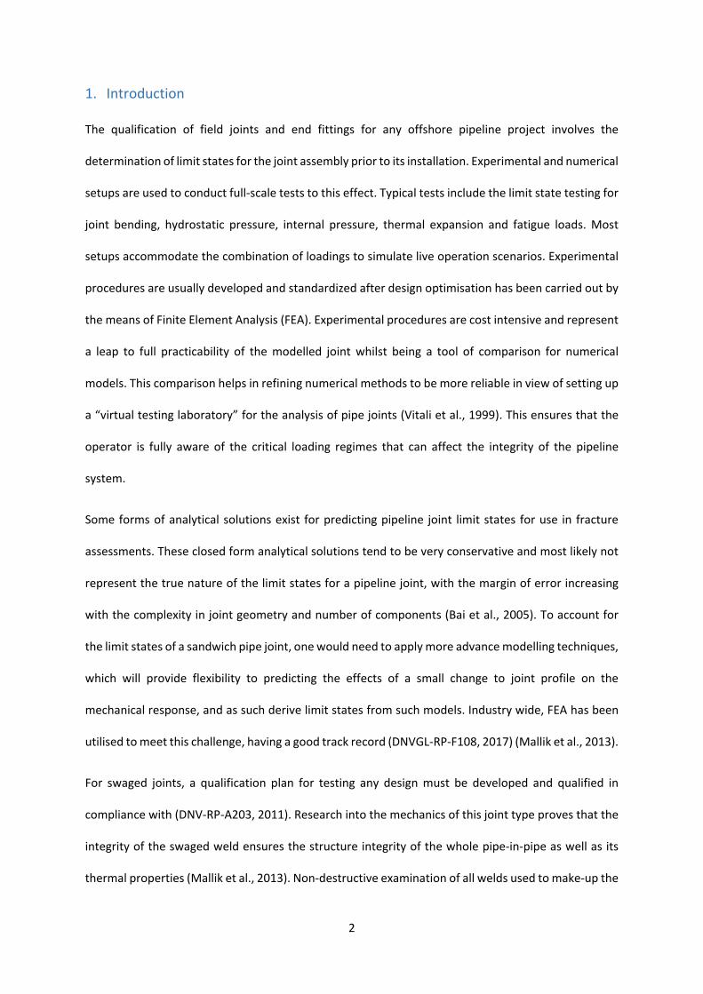
the crack face. Figure 2 outlines some of the typical installation loads.
Sensitivity analysis to
determine the worst-load case
in FEAApproach: FEA
uncracked model
Determine the severity of
defects; select the defect
positions on which ECA to
be performed.Approach: FEA
uncracked model
For each defect position,
deduce stress concentration
factor and reference
stressApproach: FEA cracked model
For each defect position, deduce
maximum acceptable
initial defect size
Approach: DNVGL-RP-F108 + FEA
Next defect position
4
2. Theory and Motivation
The fracture mechanics approach is widely used to ascertain the fracture limit state for cracks in
pipelines and pipeline girth welds. The applicability of fracture mechanics assessments can be
summarised as, firstly, deriving weld defect acceptance criteria and, secondly, evaluating fitness-for-
purpose based on the fracture limit state for both installation and operational scenarios. For pipeline
girth welds with circumferential defect, the local stress/strain state at the joint should be determined
especially in the longitudinal direction as the crack opening is primarily driven in mode I (DNVGL-RP-
F108, 2017). This means that a suitable approach must be able to account for the effect of mechanical
and geometric factors that affect the stress/strain state at the field joint. This effect can be determined
using stress/strain concentration factor solutions as stipulated in (BS 7910, 2013) or by using FEA
(Bjerke et al., 2011).
To carry out a generic fracture assessment for monotonic loading using the fracture mechanics
approach, as a basic requirement, we need to know some inputs such as: primary membrane and
bending stress, pipe/weld dimensions and tolerances, tensile properties (engineering stress-strain
curve) of pipe and weld material, critical fracture toughness, stress/strain concentration factor,
P: Hydrostatic pressure. T: Tension due to pipe weight. M: Moment due to the sagbend curvature
Figure 2 Typical loads on the pipeline during J-lay installation (Kyriakides and Corona, 2007)

5
maximum acceptable stable crack extension and residual stresses. The required inputs vary depending
on the pipeline geometry, loading scenario, environmental conditions and proposed lifetime of the
pipeline. Another important consideration is as to whether the approach is defined for load-based or
displacement-based installation conditions. Generally, scenarios where the maximum longitudinal
stress in the pipe exceeds 90% of the yield stress (0.9𝜎𝜎𝑦𝑦) are classified as strain-based and below
0.9𝜎𝜎𝑦𝑦, are classified as stress-based.
Assessment is generally made by means of a Failure Assessment Diagram (FAD) based on the principles
of fracture mechanics. The FAD (Figure 3) assesses a flaw size against a failure assessment curve,
signifying if the flaw is acceptable or not for a particular loading case. The assessment points are
plotted using the fracture ratio 𝐾𝐾𝑟𝑟 as the abscissa and the load ratio 𝐿𝐿𝑟𝑟 as the ordinate, derived for
the particular load case. The fracture ratio compares the applied loading and can be written explicitly
as:
𝐾𝐾𝑟𝑟 =𝐾𝐾𝑒𝑒𝑒𝑒𝑒𝑒𝐾𝐾𝑚𝑚𝑚𝑚𝑚𝑚
where 𝐾𝐾𝑒𝑒𝑒𝑒𝑒𝑒 is the effective stress intensity factor and 𝐾𝐾𝑚𝑚𝑚𝑚𝑚𝑚 and is the fracture toughness of the
material. The effective stress intensity factor is computed from the stress intensity factor solutions
derived from FEA as
𝐾𝐾𝑒𝑒𝑒𝑒𝑒𝑒 = �𝐾𝐾I2 + 𝐾𝐾II2 +𝐾𝐾III2
(1 − 𝜈𝜈2)
where 𝐾𝐾I,𝐾𝐾II and 𝐾𝐾III represent the Stress Intensity Factors (SIF) corresponding to mode I, II and III
respectively.
The load ratio 𝐿𝐿𝑟𝑟 is computed as:
𝐿𝐿𝑟𝑟 =𝜎𝜎𝑟𝑟𝑒𝑒𝑒𝑒𝜎𝜎𝑦𝑦
where 𝜎𝜎𝑟𝑟𝑒𝑒𝑒𝑒 is the reference stress and 𝜎𝜎𝑦𝑦 is the material yield stress. The reference stress 𝜎𝜎𝑟𝑟𝑒𝑒𝑒𝑒 is an
important parameter that allows for the prevention of plastic collapse in a given geometry under
certain loading conditions. For static loading, the reference stress is the representative stress for the
(2.1)
(2.2)
(2.3)

6
annular region from which the Stress Intensity Factor (SIF) solutions are computed and that can be
calculated analytically for a number of geometries (BS 7910, 2013), capturing the influence of the
primary membrane and bending stresses, flaw dimensions and structure size. For the swaged weld,
the reference stress is the equivalent longitudinal stress due to maximum potential loading during
installation and can only be computed using FEA.
In order to derive the failure assessment curve, detailed stress-strain data is required especially for
strains below 1%. The ordinate of the failure assessment curve points is the load ratio that is computed
as the ratio of the engineering stress to the yield stress. The required engineering stress is equivalent
to the reference stress in Eqn. (2.3) and is derived from the stress-strain data as a function of the
selected load ratio. As a minimum, 𝐿𝐿𝑟𝑟 values should be selected at 0.7, 0.9, 0.98, 1.0 and 1.02. The
abscissa of the failure assessment curve points can be derived using the expression for the “Option 2”
curve (BS 7910, 2013):
𝑓𝑓(𝐿𝐿𝑟𝑟) = �𝐸𝐸𝜀𝜀𝑟𝑟𝑒𝑒𝑒𝑒𝐿𝐿𝑟𝑟𝜎𝜎𝑦𝑦
+𝐿𝐿𝑟𝑟3𝜎𝜎𝑦𝑦
2𝐸𝐸𝜀𝜀𝑟𝑟𝑒𝑒𝑒𝑒�−0.5
𝑓𝑓𝑓𝑓𝑓𝑓 𝐿𝐿𝑟𝑟 < 𝐿𝐿𝑟𝑟,𝑚𝑚𝑚𝑚𝑚𝑚
𝑓𝑓(𝐿𝐿𝑟𝑟) = 0 for 𝐿𝐿𝑟𝑟 ≥ 𝐿𝐿𝑟𝑟,𝑚𝑚𝑚𝑚𝑚𝑚
where 𝜀𝜀𝑟𝑟𝑒𝑒𝑒𝑒 is the true strain at the true stress computed from 𝐿𝐿𝑟𝑟𝜎𝜎𝑦𝑦 for the load ratios considered and
𝐿𝐿𝑟𝑟,𝑚𝑚𝑚𝑚𝑚𝑚 =𝜎𝜎𝑢𝑢 + 𝜎𝜎𝑦𝑦
2𝜎𝜎𝑦𝑦
where 𝜎𝜎𝑢𝑢 is the ultimate tensile strength. The “Option 2” curve is suitable for all metals regardless of
the stress-strain behaviour as it captures the non-linearity in the stress-strain curve.
In the absence of tearing resistance data for the swage weld geometry, the methodology described
above can only be applied when using the Linear Elastic Fracture Mechanics (LEFM) theory and
assumptions (Sun and Jin, 2012). In other words, the small-scale yielding assumption is valid for this
approach. Small-scale yielding simply implies that the region of inelastic deformation at the crack tip
is well within the zone dominated by the LEFM asymptotic solution. This allows for the
characterisation of the local crack-tip stress field using solely the elastic stress intensity factor 𝐾𝐾, which
is a function of the applied stress, the location and size of the crack and the geometry of the pipe joint
(2.4)
(2.5)
(2.6)

7
(Zehnder, 2012). In other words, 𝐾𝐾 defines a stress profile near the crack tip that upon reaching a
critical state signifies a small crack extension and subsequent material failure. This critical state is
denoted by a value 𝐾𝐾𝑚𝑚𝑚𝑚𝑚𝑚, also known as the fracture toughness of a material (critical value of 𝐾𝐾
required to initiate crack growth). This theory works well for brittle materials; as for ductile materials,
we know that the fracture toughness is a function of the crack extension and we would need a tearing
resistance curve, where the crack driving force is a function of the crack extension, to appropriately
predict stable tearing (Pisarski et al., 2006).
Determining the material fracture toughness measured by J-methods, 𝐽𝐽𝑚𝑚𝑚𝑚𝑚𝑚 of a material (Zhu and
Joyce, 2012) allows us to obtain the critical fracture toughness for a linear elastic material under quasi-
static conditions and plane strain (gives the practical minimum value):
𝐾𝐾𝑚𝑚𝑚𝑚𝑚𝑚 = �𝐽𝐽𝑚𝑚𝑚𝑚𝑚𝑚𝐸𝐸1 − 𝑣𝑣2
where 𝐸𝐸 and 𝜈𝜈 are the elastic modulus and Poisson’s ratio respectively.
Calculations for a flaw provide the co-ordinates either of an assessment point or, in the case of crack
growth, a locus of points. These points are then compared with the failure assessment curve to
determine the acceptability of the flaw. A simple illustration of this methodology for a circumferential
crack (of depth 𝑎𝑎) in a pipe in tension is shown in Figure 3(a), where defects corresponding to
assessment points that lie outside the failure assessment curve are deemed unacceptable. For a
surface crack in a plate under axial loading, the elastic SIF solutions from FEA show good agreement
with analytical solutions (BS 7910, 2013) as illustrated in Figure 3(b).
(2.7)

8
Figure 3 (a) FAD assessment points and a failure assessment curve (FAC) for a pipe with circumferential crack in tension;
(b) Elastic SIF comparison
For pipeline girth welds and tubular fillet welds there exist, in form of codes and standards (BS 7910,
2013, API-579-1/ASME-FFS-1, 2016), a compendium of detailed reference stress and SIF solutions. For
the specific geometry of the swage weld, the SIF and reference stress inputs required for the ECA can
only be obtained by FEA and as such, the studies carried out in this paper utilise only FEA
methodologies. Several studies have applied the FEA approach to arrive at unique solutions to
“standard-exempted” problems. In (Bjerke et al., 2011), a simplified procedure was introduced for
performing more accurate prediction of the crack driving force based on (DNV-OS-F101, 2007) by using
3D FEA. In (O�stby, 2005), an equation was derived to calculate the applied crack driving force in terms
of J-integral or crack tip opening displacement for pipes with surface cracks based on 2D and 3D FEA;
taking into account the effect of biaxial loading, yield stress mismatch and misalignment. Using large-
scale 3D FEA-based parametric studies, in (Kibey et al., 2010) closed-form strain capacity equations
were derived, which were then utilised for strain based design ECA procedures for welded pipelines.
In response to the geometric limitations of the stress intensity factor and reference stress solutions as
documented for pipe joint types in recommended practice standards, finite element fracture
mechanics methods have been long utilised to capture the stress state for different combinations of
0
0.5
1
1.5
2
2.5
3
0 0.5 1 1.5 2
Kr
Lr
FAC
a=1mm
a=2mm
a=3mm
a=4mm
(a)0
100
200
300
400
500
600
0 2 4 6 8 10
SIF
(N/m
m3/
2 )Defect depth (mm)
FEA
Analytical
(b)
Unacceptable
Acceptable

9
defects in unique joint types (Arun et al., 2014, Kibey et al., 2010, Bell et al., 1985). In addition, it is
used to confirm the validity and hence conservatism of analytical procedures (Bjerke et al., 2011). No
documentation of the utilization of finite element fracture mechanics for the swaged weld has been
published and the influence of the core and filler resin load-carrying capacity on the fracture
assessment outcomes of the swage weld remains unknown.
This paper seeks to apply a combination of techniques with the aim of outlining a FEA-based
methodology for carrying out ECA on the swage weld for J-lay installation. In the first section, in other
to avoid carrying out ECA on all potential defect positions, the stress profile at the swaged weld is
examined to determine the most severe defect position as a function of the stress concentration.
Closed-form parametric equations for quantifying the geometric Stress Concentration Factor (SCF) as
a function of the swage weld dimensions are derived using large-scale parametric studies and
statistical analysis for the joint under tension. For unique joint types, FEA methodologies can indeed
be used to derive such equations (Morgan and Lee, 1998), and such solutions can be considered
adequate in the absence of full experimental results. The FEA methodology to determine the crack
driving force and the acceptable flaw size for the swage weld in a sandwich pipe joint is outlined based
on procedures in (DNVGL-RP-F108, 2017) and (API-579-1/ASME-FFS-1, 2016).
3. Analysis of critical defect position
The distribution of stress about the swage weld toe is known to be a major consideration in both the
fracture and fatigue assessment of swaged jointed pipe-in-pipe systems (Mallik et al., 2013). During
offshore installation, the sandwich pipe joint would have to withstand the reaction force from the
tensioner due to the weight of the submerged part of the pipe assembly and a bending moment at
the sagbend just before being laid on the seabed. With respect to these loadings, stress concentration
around the swaged weld toe is expected due to the change in geometry and strength mismatch
between the weld metal and the pipe metal, all which cause stress discontinuities.

10
For the sandwich pipe swage joint the geometrically induced stress concentration can be quantified
using the so-called Stress Concentration Factor (SCF) defined as:
SCF =maximum stress in region of interest
stress in component without stress riser
The geometry of the connection and swaged weld is shown in Figure 4 for a discontinuous annulus
joint type (meaning there is no continuous transfer of load between two adjacent outer pipes, only
through the swage weld).
Figure 4 Configuration of a sandwich pipe field joint
The regions must first be classified in order of stress severity under loadings to determine the worst
scenario model. For this, a base model is built with properties as stated in Table 1.
Table 1 Properties of base model
Young’s modulus
𝐸𝐸 (GPa)
Poisson’s ratio
𝜈𝜈
Radius
𝑓𝑓 (mm)
Thickness
𝑡𝑡 (mm)
Inner pipe 205 0.3 109.55 12.7
Outer pipe 205 0.3 161.95 12.7
Swaged weld 207 0.3 n/a n/a
Filler resin
Outer pipe
Annular core
Swaged weld
Inner pipe
(3.1)

11
The entire analysis is based on linear elastic deformation only. Considering a model of the swaged
weld joint in tension, we can express a consistent statistical through thickness stress distribution in
terms of a membrane component 𝜎𝜎𝑚𝑚 and a bending component 𝜎𝜎𝑏𝑏 as seen in Figure 5(a), which add
up to give the nominal stress 𝜎𝜎𝑛𝑛. The peak stress 𝜎𝜎𝑝𝑝𝑒𝑒𝑚𝑚𝑝𝑝 can be described as the product of the
geometric SCF and 𝜎𝜎𝑛𝑛. This represents a local through-thickness normal and shear stress distribution
at the swaged weld toe. The potential defect positions as highlighted by (Mallik et al., 2013) are
marked in Figure 5(b).
Figure 5 (a) Geometry of the swage weld; (b) Locations for potential defects
Similar studies carried out on a conventional pipe-in-pipe subjected to J-lay installation loads revealed
that the weld toe (location A) would experience the highest stress concentration relative to the other
locations (Dixon et al., 2003). In preliminary fracture assessment, this location is recognised to be a
potential failure location in the presence of fabrication imperfections and is usually taken as the limit
region for the joint. This is the first step in the ECA, and for an installation case, the fracture assessment
is of more concern to us. Indeed having an idea of the stress distribution and peak stresses that would
occur at the swaged weld toe would be a great first step to understanding just how the fracture
assessment criteria will be established.
𝜎𝜎𝑛𝑛 𝜎𝜎𝑝𝑝𝑒𝑒𝑚𝑚𝑝𝑝
𝜏𝜏(𝑦𝑦)
𝜎𝜎𝑚𝑚 𝜎𝜎𝑏𝑏
F
M
(a)
A B F
(b)

12
Figure 6 Axisymmetric finite element model
The finite element software ABAQUS (ABAQUS, 2014) was used for all load cases in this study. Under
axial loading, the base model was subjected to 60% of its axial capacity as described in (API-RP-1111,
2015), with perfect bonding assumed between the interlayers of the sandwich pipe. Since the
geometry and loading of the given case satisfy rotational symmetry, axisymmetric models with CAX4
elements (4-node bilinear axisymmetric quadrilaterals) were used to capture this behaviour. In view
of the perfect bonding assumption between the interlayers, one would be able to define the
installation tension as an equally distributed force acting at the pipe ends as seen in Figure 6.
Geometric partitions were made about the potential defect locations and mesh refinement applied.
The partition length 𝑝𝑝𝑙𝑙 = �𝑓𝑓𝑚𝑚𝑡𝑡1 was chosen as the meridional length for local stress classification as
specified in (ASME BPVC-VIII-2, 2015) where 𝑓𝑓𝑚𝑚 and 𝑡𝑡1 are the inner pipe mid surface radius and
thickness respectively. A generic mesh convergence study was carried out to ascertain the change in
the peak stress with mesh density as seen in Figure 7(a). Since the measure of “stress” as we limit the
X-symm B.C Y-symm B.C
axis of rotational symmetry
X
Y
𝒕𝒕𝟏𝟏
𝒑𝒑𝒍𝒍
600mm
250mm

13
mesh size to infinitesimal values in elastic analysis will approach infinity and thus unrealistic, an
instability criterion was defined in ABAQUS to calculate the Load Proportionality Factor (LPF) at the
first instability at the swaged weld region. The mesh density was normalised by its lowest value in the
sample set. A typical result can be seen in Figure 7(b), showing the stress distributions around the
swaged weld.
Figure 7 (a) Variation of peak stress with normalised mesh density; (b) Stress contour plot of swage weld (red contour: peak stress)
The stress linearization technique outlined in (ASME BPVC-VIII-2, 2015) was utilised via the stress
classification line. The stress classification line for each potential defect position was chosen to be
perpendicular to its mode I opening direction. The longitudinal membrane plus bending stress
component was computed and compared with results obtained by (Mallik et al., 2013) where the
stress severity ranking by location was A, B, C, D. The results obtained in this study can be seen in
Table 2.
0.00
1.00
2.00
3.00
4.00
5.00
6.00
7.00
8.00
9.00
0
5
10
15
20
25
0 5 10
LPF
Peak
stre
ss, %
diff
eren
ce
Normalised mesh density(a) (b)
14
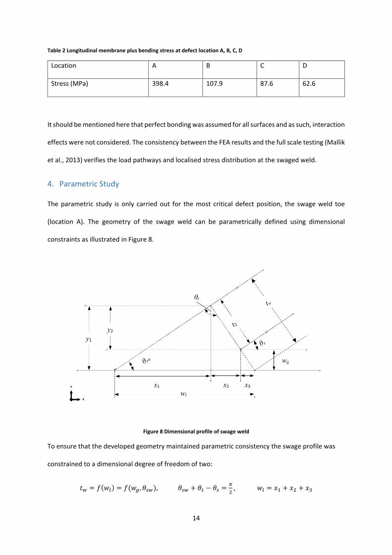
Table 2 Longitudinal membrane plus bending stress at defect location A, B, C, D
Location A B C D
Stress (MPa) 398.4 107.9 87.6 62.6
It should be mentioned here that perfect bonding was assumed for all surfaces and as such, interaction
effects were not considered. The consistency between the FEA results and the full scale testing (Mallik
et al., 2013) verifies the load pathways and localised stress distribution at the swaged weld.
4. Parametric Study
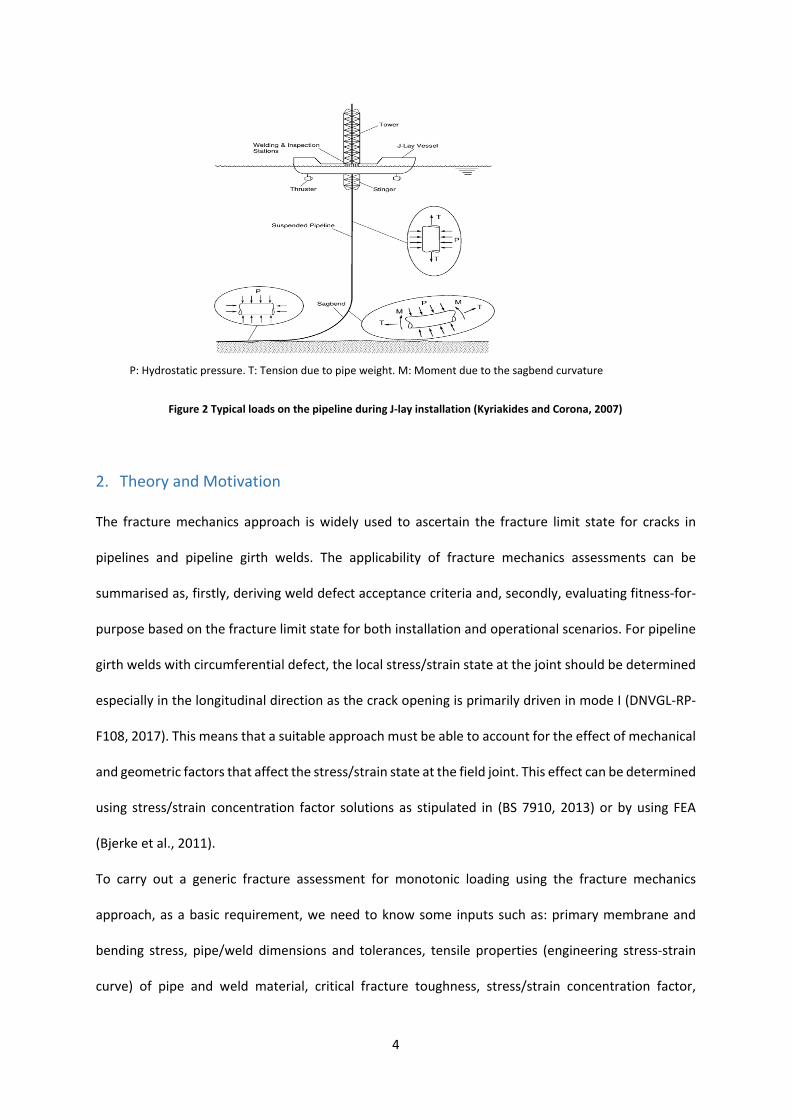
The parametric study is only carried out for the most critical defect position, the swage weld toe
(location A). The geometry of the swage weld can be parametrically defined using dimensional
constraints as illustrated in Figure 8.
Figure 8 Dimensional profile of swage weld
To ensure that the developed geometry maintained parametric consistency the swage profile was
constrained to a dimensional degree of freedom of two:
𝑡𝑡𝑤𝑤 = 𝑓𝑓(𝑤𝑤𝑙𝑙) = 𝑓𝑓(𝑤𝑤𝑔𝑔, 𝜃𝜃𝑠𝑠𝑤𝑤), 𝜃𝜃𝑠𝑠𝑤𝑤 + 𝜃𝜃𝑚𝑚 − 𝜃𝜃𝑠𝑠 = 𝜋𝜋2
, 𝑤𝑤𝑙𝑙 = 𝑥𝑥1 + 𝑥𝑥2 + 𝑥𝑥3
wg
x2 x3 wl
x1
θt
y1 y2

15
The resulting geometric equations then become input functions for the parametric scripts
𝑦𝑦1 = 𝑤𝑤𝑔𝑔 + sin �𝜋𝜋2− 𝜃𝜃𝑠𝑠� 𝑡𝑡2 (4.1)
𝑥𝑥1 = 𝑦𝑦1tan𝜃𝜃𝑠𝑠𝑠𝑠
(4.2)
𝑥𝑥2 = 𝑡𝑡2 cos �𝜋𝜋2− 𝜃𝜃𝑠𝑠� (4.3)
𝑥𝑥3 = 𝑤𝑤𝑔𝑔
tan�𝜋𝜋2−𝜃𝜃𝑠𝑠� (4.4)
𝑤𝑤𝑙𝑙 =𝑤𝑤𝑔𝑔+sin�𝜋𝜋2−𝜃𝜃𝑠𝑠�𝑚𝑚2
tan𝜃𝜃𝑠𝑠𝑠𝑠+ 𝑡𝑡2 cos �𝜋𝜋
2− 𝜃𝜃𝑠𝑠� + 𝑤𝑤𝑔𝑔
tan�𝜋𝜋2−𝜃𝜃𝑠𝑠� (4.5)
𝑡𝑡𝑤𝑤 = 𝑡𝑡2 + 𝑤𝑤𝑔𝑔
sin�𝜋𝜋2−𝜃𝜃𝑠𝑠�= 𝑤𝑤𝑙𝑙 sin(𝜃𝜃𝑠𝑠𝑤𝑤) (4.6)
The selected range of material and geometric parameters used for parametric study can be found in
Table 3. The range of 𝐸𝐸𝑐𝑐𝑝𝑝 (core-to-pipe elastic modulus ratio), 𝐸𝐸𝑟𝑟𝑝𝑝 (resin-to-pipe elastic modulus
ratio) and 𝐸𝐸𝑤𝑤𝑝𝑝 (weld-to-pipe elastic modulus ratio) was chosen based on upper and lower bound
limits that are practically applicable. The range of 𝑤𝑤𝑙𝑙 (swaged weld length) and 𝑤𝑤𝑔𝑔 (swaged weld
gap) was chosen based on reported samples as fabricated by (Mallik et al., 2013).
Table 3 Range of parameters used in the parametric study
𝐸𝐸𝑐𝑐𝑝𝑝 𝐸𝐸𝑟𝑟𝑝𝑝 𝐸𝐸𝑤𝑤𝑝𝑝 𝑤𝑤𝑙𝑙 (mm) 𝑤𝑤𝑔𝑔 (mm) 𝑡𝑡1 𝑓𝑓1⁄
0.001 0.001 0.8 25 3 0.12
0.005 0.005 0.9 30 6 0.15
0.01 0.01 1.0 35 9 0.17
0.05 0.05 1.1 40 12 0.20
0.1 0.1 1.2 45 15

16
4.1. Influence of swage weld length
The swage weld length 𝑤𝑤𝑙𝑙 is the main design parameter that determines just how much weld metal
is deposited to form the connection and is a direct function of the angular difference between the
outer pipe swage angle and the swage weld angle. Two different sets of core and resin stiffness are
examined with the weld gap fixed in all design models. Figure 9 shows the influence of the swage
weld length on the SCF. It can be seen that increasing the weld length reduces the SCF at the swage
weld toe. This is directly related to the increased surface area of the weld, meaning it will be able to
carry more load. This is obviously a simplistic approach as other fabrication, inspection and
geometric tolerances would constrain the actual weld length that can be utilised for a swage
connection.
(a) (b)
Figure 9 Influence of weld length 𝒘𝒘𝒍𝒍 on SCF for a range of resin-to-pipe elastic modulus ratios 𝑬𝑬𝒓𝒓𝒑𝒑:
(a) Continuous annulus; (b) Discontinuous annulus
4.2. Influence of swage weld gap
The weld gap 𝑤𝑤𝑔𝑔 directly influences the evolution of compressive stresses at the throat of the swage
weld. These compressive stresses are magnified as the weld gap reduces and have an inverse
relationship with the tensile stresses at the swage weld toe. Therefore, as the weld gap increases, the
compressive stresses at the throat decreases and this amplifies the tensile stresses around the swage
0
0.2
0.4
0.6
0.8
1
1.2
1.4
20 30 40 50
SCF
Weld length (mm)
Erp=0.001Erp=0.01Erp=0.1
0
0.5
1
1.5
2
2.5
3
3.5
20 30 40 50
SCF
Weld length (mm)
Erp=0.001Erp=0.01Erp=0.1

17
weld toe (Figure 10). The welding residual stresses would definitely have a significant effect on the
stress distribution around the swage weld and should be considered during detailed design of the
joint.
Figure 10 Influence of weld gap 𝒘𝒘𝒈𝒈 on SCF for a range of resin-to-pipe modulus ratios 𝑬𝑬𝒓𝒓𝒑𝒑:
(a) Continuous annulus (b) Discontinuous annulus
4.3. Influence of thickness to radius ratio
We can see from Figure 11(a) that the influence of the inner pipe thickness to radius ratio 𝑡𝑡1 𝑓𝑓1⁄ on
the SCF is as expected. As 𝑡𝑡1 𝑓𝑓1⁄ increases, the SCF reduces for all sampled weld lengths, because the
pipe’s cross sectional area increases also. The stiffer the weld metal, the higher the SCF will be simply
due to the preferential deformation of the inner pipe at the interface with the weld (Figure 11(b)). The
advantage of having continuous load transfer between adjacent outer pipes can be seen from the
results for continuous and discontinuous annulus type joints as the SCF is always lower for continuous
annulus joints. Although this requires additional weld connections being made during installation,
which subsequently increases the offshore time and the installation cost.
0
0.2
0.4
0.6
0.8
1
1.2
1.4
0 5 10 15 20
SCF
Weld gap (mm)
Erp=0.001Erp=0.01Erp=0.1
(a)0
0.5
1
1.5
2
2.5
3
0 5 10 15 20
SCF
Weld gap (mm)
Erp=0.001Erp=0.01Erp=0.1
(b)

18
Figure 11 (a) Influence of the inner pipe thickness-to-radius ratio 𝒕𝒕𝟏𝟏 𝒓𝒓𝟏𝟏⁄ on SCF for a range of weld lengths 𝒘𝒘𝒍𝒍 (discontinuous annulus);
(b) Influence of weld-to-pipe elastic modulus ratio 𝑬𝑬𝒘𝒘𝒑𝒑 on SCF for a range of resin-to-pipe elastic modulus ratios 𝑬𝑬𝒓𝒓𝒑𝒑 (continuous annulus)
4.4. SCF Correlations
Considering the wide range of geometric parameters involved in the analysis of the stress state at
the swage weld, it would be cumbersome to try to develop simple equations that can accurately
predict the SCF at the weld toe for all possible configurations. Using the results from 12500 FE
models, a set of fitted correlations were derived to predict the SCF at the weld toe and quantify the
geometrically induced stress magnification. This approach is only applicable for elastic analysis and
axial load cases (e.g. tension due to pipe weight during installation). The below listed correlations
exclusively quantify the influence of the geometric and elastic material properties on the SCF and as
such the accuracy is not a function of the remote axial loads as long as there is no plastic
deformation. In addition, the perfect adhesion assumption holds true for these correlations, hence
the transfer of load between pipe-core, pipe-weld and pipe-resin is continuous.
The models were automatically generated using a script file with the geometric parameters shown in
Figure 8 and given in Eqns. (4.1) – (4.6) and parameter values listed in Table 3. To arrive at the full
model sets, each parameter value in Table 3 is used in combination with other parameters for the
0
0.5
1
1.5
2
2.5
3
3.5
0.1 0.12 0.14 0.16 0.18 0.2 0.22
SCF
Inner pipe thickness-to-radius ratio
wl=25mm wl=30mmwl=35mm wl=40mmwl=45mm
0
0.2
0.4
0.6
0.8
1
1.2
0.8 0.9 1 1.1 1.2
SCF
Weld-to-pipe elastic modulus ratio
Erp=0.001Erp=0.005Erp=0.01Erp=0.05Erp=0.1
(b)

19
four sampled values of 𝑡𝑡1 𝑓𝑓1⁄ yielding (4 × 55) = 12500 model sets. A python script file was utilized
for the automated model input file generation, creation of an array of input files that varied one
parameter against the others and submission of the analysis jobs. A SLURM script (Yoo et al., 2003)
was then utilised to run the python script file on a supercomputer cluster. Afterwards, the maximum
longitudinal stress values at the swaged weld toe were extracted from the output database file using
a predefined node set embedded in a modified python file (compatibility was not a problem as the
mesh was the same for all models) run in the python development environment of ABAQUS. The
extracted results were then copied to the analysis module of (SigmaPlot, 2014) where the data was
fitted to yield correlations to the FE results and generate shared parameters between data sets
which are then used to generate scaling factors as a function of the sampled parameter.
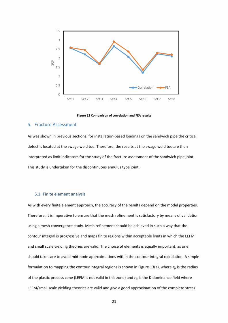
Results from the correlations proposed below were compared with results from finite element
analysis. To capture the variation of the input parameters extensively, a parameter randomization
function was incorporated in the script used to generate the model input files. The variation in both
results is seen in Figure 12 for eight random parameter datasets.
The following equations are valid for 1.0 ≤ 𝑤𝑤𝐿𝐿 𝑡𝑡𝑤𝑤⁄ ≤ 2.0 , 0 < 𝑤𝑤𝑔𝑔 𝑡𝑡𝑤𝑤⁄ ≤ 0.5:
SCF = 𝑎𝑎𝑎𝑎𝑎𝑎𝑒𝑒(1 + 𝑤𝑤𝑙𝑙𝑚𝑚𝑠𝑠
)−𝑑𝑑 (4.7)
𝑎𝑎 = −3.53 − 2.466 ln(𝐸𝐸𝑟𝑟𝑝𝑝 + 0.01018) (4.8)
𝑎𝑎 = 𝑏𝑏(𝑖𝑖)
𝑏𝑏∗ (4.9)
where
𝑎𝑎∗ = 3.7776 �𝑤𝑤𝑙𝑙𝑚𝑚𝑠𝑠�−0.631
(4.10)
𝑎𝑎(𝑖𝑖) = 𝑎𝑎′ �𝑤𝑤𝑙𝑙𝑚𝑚𝑠𝑠�−𝑏𝑏′′
(4.11)
𝑎𝑎′ = 3.097 − 0.1702 ln(𝐸𝐸𝑐𝑐𝑝𝑝 + 0.00831) (4.12)

20
𝑎𝑎′′ = 0.3264 − 0.0777 ln(𝐸𝐸𝑐𝑐𝑝𝑝 + 0.009829) (4.13)
𝑎𝑎 = 0.7683(1.941)𝑠𝑠𝑔𝑔𝑡𝑡𝑠𝑠 (4.14)
𝑑𝑑 = 1.0233exp�−9.526𝐸𝐸𝑟𝑟𝑝𝑝� (4.15)
𝑒𝑒 = 0.2304exp �11.976 𝑚𝑚2𝑟𝑟2� �𝑚𝑚1
𝑟𝑟1��1.0525𝑡𝑡2𝑟𝑟2
−0.2726� (4.16)
Through thickness variation
The equation is valid for 1.0 ≤ 𝑤𝑤𝑙𝑙 𝑡𝑡𝑤𝑤⁄ ≤ 2.0, 𝑓𝑓𝑖𝑖 ≥ 𝑓𝑓𝑚𝑚, 𝜑𝜑 = 1 for 𝑓𝑓𝑖𝑖 = 𝑓𝑓𝑚𝑚 for all 𝑤𝑤𝑙𝑙 𝑡𝑡𝑤𝑤⁄ . Parameter 𝜑𝜑
defines a stress decay parameter, where the stress at a point 𝑓𝑓𝑚𝑚 is
𝜎𝜎𝑟𝑟𝑚𝑚 = 𝜑𝜑 ∗ SCF ∗ remotely applied stress
𝜑𝜑 =−1.025+�𝑟𝑟𝑚𝑚𝑟𝑟𝑖𝑖
�
−𝑒𝑒+𝑔𝑔�𝑟𝑟𝑚𝑚𝑟𝑟𝑖𝑖�ℎ (4.17)
𝑓𝑓 = 3.8737 �𝑚𝑚1𝑟𝑟1�0.2124
(4.18)
𝑔𝑔 = 3.8513 �𝑚𝑚1𝑟𝑟1�0.2145
(4.19)
ℎ = �0.2995 �𝑤𝑤𝑙𝑙𝑚𝑚𝑠𝑠� + 0.4765�+0.707ln �𝑟𝑟𝑚𝑚
𝑟𝑟𝑖𝑖� (4.20)
21
Figure 12 Comparison of correlation and FEA results
5. Fracture Assessment
As was shown in previous sections, for installation-based loadings on the sandwich pipe the critical
defect is located at the swage weld toe. Therefore, the results at the swage weld toe are then
interpreted as limit indicators for the study of the fracture assessment of the sandwich pipe joint.
This study is undertaken for the discontinuous annulus type joint.
5.1. Finite element analysis
As with every finite element approach, the accuracy of the results depend on the model properties.
Therefore, it is imperative to ensure that the mesh refinement is satisfactory by means of validation
using a mesh convergence study. Mesh refinement should be achieved in such a way that the
contour integral is progressive and maps finite regions within acceptable limits in which the LEFM
and small scale yielding theories are valid. The choice of elements is equally important, as one
should take care to avoid mid-node approximations within the contour integral calculation. A simple
formulation to mapping the contour integral regions is shown in Figure 13(a), where 𝑓𝑓𝑝𝑝 is the radius
of the plastic process zone (LEFM is not valid in this zone) and 𝑓𝑓𝑝𝑝 is the K-dominance field where
LEFM/small scale yielding theories are valid and give a good approximation of the complete stress
0
0.5
1
1.5
2
2.5
3
3.5
Set 1 Set 2 Set 3 Set 4 Set 5 Set 6 Set 7 Set 8
SCF
Correlation FEA

22
field (ABAQUS, 2014). To avoid conservatism, one can define the contour integrals in such a way that
it is progressive and bound between these two zones. The FE package ABAQUS was used to undergo
all case studies. It offers three different criteria for isotropic linear elastic materials namely: the
maximum tangential stress criterion, the maximum energy release rate criterion and the 𝐾𝐾II = 0
criterion. Although these criteria, like most general loading theories, assume that crack extension
occurs with 𝐾𝐾II = 0, they do vary slightly with the prediction of crack initiation angle (Dassault
Systèmes, 2012). The simplest estimation of the plastic zone size can be obtained from the elastic
solution of the sharp crack problem. For characteristic crack length 𝑎𝑎, the definition of a finite zone
𝑓𝑓𝑝𝑝 in which K-field dominates needs to satisfy the criterion (Dassault Systèmes, 2012):
𝑎𝑎5
> 𝑓𝑓𝑝𝑝 > 3𝑓𝑓𝑝𝑝 ≈12�𝐾𝐾IC𝜎𝜎𝑦𝑦�2
where 𝐾𝐾IC is the critical stress intensity factor for mode I fracture and 𝜎𝜎𝑦𝑦 is the material yield stress.
The computed plastic zone size is based on Irwin’s suggestion for mode I fracture (Irwin, 1961).
The J-integral method is also achievable using FE analysis, where for linear elastic materials; the J-
value can be used to represent the energy release rate 𝐺𝐺, associated with crack growth. Applying
small scale yielding assumptions, the contour for the J-integral (𝜆𝜆) will fall within the region in which
LEFM is valid as shown in Figure 13(a). Thus, for a linear elastic material the following is valid (plane
strain):
𝐽𝐽 = 𝐺𝐺 =1 − 𝑣𝑣2
𝐸𝐸𝐾𝐾I2
The theory behind the FE computation of the SIF and J-integral is detailed in (ABAQUS, 2014).
Modelling of the crack within the pipe can be done using a defined seam for sharp cracks with
infinitesimal length in the axial direction or a blunt semi-elliptical crack with open geometry as
shown in Figure 13(b) for a pipeline girth weld with misalignment. Sharp cracks are best suited for
small-strain analysis and care should be taken in interpreting the singularity behaviour at the crack
(5.1)
(5.2)

23
tip. On the other hand, blunted cracks are best suited for finite-strain analysis, and depending on the
defined crack tip profile, non-singular behaviour is possible. In a case where non-linear material
response is considered, the results become more sensitive to the mesh profile and as such, it is
advisable to use finer mesh profiles. The contour integral grows outwards from the crack tip to a
finite region within the pipe depending on the number of output requests, and as such, it is
important to read off the results from a contour that falls within the K-dominance zone. At the crack
tip, the elements represented by degenerated quads should be utilised for sharp cracks. The
degeneration is controlled by collapsing one side of the second-order quad elements to a single
point at the crack tip and then adjusting the mid-side nodes to move closer to the crack tip by a
parameter 𝑡𝑡; arriving at a mesh that allows for accurate prediction of the stress singularity at the
crack tip. Since the mid-side node parameter actively adjust the nodes on the seam elements, care
should be taken when choosing its value. To avoid producing screwed elements (especially for FE 3D
fracture mechanics analyses), a sensitivity study should be carried out to ascertain the minimal value
for 𝑡𝑡 that would not lead to analysis errors. Results outside this zone usually show inconsistency and
as such should be avoided (Dassault Systèmes, 2012). It is well known that there exist an angular
dependence for the stress/strain field around the crack tip and as such, we require a reasonable
number of elements to obtain a good angular resolution. Subtend angles in the range of 10° − 20°
around the crack tip were found to accurately obtain reasonable results for LEFM.

24
Figure 13 (a) Dominance fields (b) Validation model
5.2. Model Validation
To validate the proposed finite element methodology, a pipeline girth welded joint was modelled to
replicate the analytical SIF and crack driving force solutions as outlined in DNV-GL F108 and BS 7910.
Different crack depths were studied whilst also taking into consideration the influence of a 1 mm high-
low characterising radial misalignment at the weld. The crack was positioned at the middle of the
weld, extending through thickness as shown in Figure 13(b). The crack driving force was calculated
using the expression:
crack driving force = 𝐾𝐾I2(1 − 𝑣𝑣2)
𝐸𝐸. 𝑓𝑓(𝐿𝐿𝑟𝑟)
Where 𝐾𝐾I represents the mode I stress intensity factor for the flaw size and geometry considered and
𝑓𝑓(𝐿𝐿𝑟𝑟) is defined as in Eqn. (2.3) making it dependent on the material stress-strain curve (Figure 14b).
Figure 14(a) shows the comparison between the FEA and analytical results for a full circumferential
rp
λ
rk Annular bounds for K-dominance
Transition zone
(a) (b) High-low
Contour rings
Crack tip
Sharp crack
Blunt crack
(5.3)

25
crack in a pipe. From the results, we see that the analytical method and FEA method differ mainly in
the prediction of the misalignment effect. The linear relationship between the crack driving force and
the crack depth signifies that the reference stress solution remained within the elastic limit of the
material for the analytical method. In addition, the analytical method does not capture the varying
effect of the misalignment on the reference stress whereas the FEA method does. This explains the
disparities in the results, as the FEA method captures the increased influence of the misalignment on
the reference stress as the crack depth increases.
Figure 14 (a) Comparison of crack driving force results (b) Stress-strain curve
As this study focuses on installation loads, each load variant will be analysed (for SIF solutions)
separately as monotonic load. The load case description are as follows:
• Full Pipe Tension (FPT): Both pipes bear the tension due to their respective submerged
weights.
• Full Pipe Moment (FPM): Curvature control for sagbend.
• Installation Case (IC): External pressure, tension due to pipe weight and moment due to
installation curvature; all applied as individual monotonic loads.
0
2
4
6
8
10
12
14
16
18
20
0 2 4 6 8 10 12
Crac
k dr
ivin
g fo
rce
(N/m
m)
Crack depth (mm)
FEA
DNVGL-F108
0
100
200
300
400
500
600
700
800
900
0 0.05 0.1 0.15 0.2
Stre
ss (M
Pa)
Strain
Engineering stress/strain
True stress/strain
(a) (b)

26
5.3. Swage Weld Model
The mesh profile for typical fully embedded circumferential seam crack located at the swage weld toe
is presented in Figure 15. To obtain accurate contour integral results for a crack in three-dimensional
analysis, care has to be taken to ensure that the mesh conforms to the cracked geometry, the crack
front is explicitly defined and the appropriate virtual crack extension direction is chosen (ABAQUS,
2014). The crack front is defined as a node set and the virtual crack extension direction is specified to
be orthogonal to the crack front tangent and the normal to the crack plane. Due to symmetry, only a
quarter of the joint assembly was modelled. Wedge elements are created along the crack tip and a
partitioning strategy ensured that the contour integral could be properly mapped within the limits for
LEFM. The crack growth direction was specified to be normal to the theta plane, to ensure that the
displacement vectors were captured within the rotational symmetry. C3D20 elements were used to
model the joint assembly with crack line element mid-side nodes moved one-fourth points along the
edge plane. Using these elements automatically implies that no mid-side nodes exist at the mid-plane
and as such, no singularity would be represented within the element, which creates differences in
interpolation between the mid-plane and edge planes leading to local oscillation of J-integral values
along the crack line.
Figure 15 Swage joint mesh profile
Wedge element Tubular domain integral along crack front

27
Base case installation loading on a sandwich pipe for a typical J-lay and other fixed design parameters
are listed in Table 4. As mentioned earlier the loads are treated as monotonic loads applied to the
joint assembly. Figure 16 shows the influence of the core-to-pipe and resin-to-pipe stiffness ratios (𝐸𝐸𝑐𝑐𝑝𝑝
and 𝐸𝐸𝑟𝑟𝑝𝑝) on the SIF and corresponding J-value for a sharp crack positioned at the swage weld toe of a
joint assembly located at the apex of the sagbend. The J-integral and SIFs are computed directly in
ABAQUS about five contour intervals and the reported values are the average of the last three
intervals as the first two intervals produced significantly undulating values and as such not path
independent. The contour for the extraction of the J-value (𝜆𝜆 in Figure 13a) was chosen to fall entirely
within the annular region for K-dominance.
For the modelling of isotropic materials with the perfect adhesion assumption, the load bearing
capacity of the sandwich pipe joint under elastic bending load is simply the combination of the load
bearing capacities of the layers. Therefore, at constant load, the influence of the core and filler resin
stiffness on the elastic SIF for a crack located at the swaged weld toe can be simply quantified by the
variation in stress state in the K-field domain around the crack tip. The better the load bearing
properties of the annular materials, the lesser the stress state at constant load, and the lesser the
elastic SIF.
The close to logarithmic relationship is expected as perfect adhesion was assumed between contacting
surfaces meaning that for this ideal case of LEFM, the relative displacement of the crack faces leading
to mode I, II and III opening is arrested by the consolidated interlayer stresses which are a direct
function of the resin stiffness. It was also discovered, that for mode I and mode II, the elastic SIF is
highest for a relatively stiffer core due to the bending stiffness mismatch effect (Onyegiri and
Kashtalyan, 2017) which is more significant for discontinuous annulus type joints.

28
Table 4 Base case installation parameters
Parameter Value Unit Comments
𝑊𝑊𝑑𝑑 3000 m Water depth
𝑊𝑊𝑠𝑠 156.32 kg/m Total submerged weight
𝑇𝑇 5479 kN Required top tension (Bai and Bai, 2005)
𝑘𝑘𝑠𝑠𝑚𝑚𝑔𝑔𝑏𝑏𝑒𝑒𝑛𝑛𝑑𝑑 0.003491 1/m Sagbend curvature (Bai and Bai, 2005)
𝑡𝑡1, 𝑡𝑡2 12.7 mm Required wall thickness for collapse check for
𝐸𝐸𝑟𝑟𝑝𝑝 = 𝐸𝐸𝑐𝑐𝑝𝑝 = 0.01 (Arjomandi and Taheri, 2011)
(𝑓𝑓1, 𝑓𝑓2) (109.55,161.95) mm Inner and outer pipe radius
𝜎𝜎𝑦𝑦 552 MPa Pipe yield stress
𝐾𝐾𝑚𝑚𝑚𝑚𝑚𝑚 65 MPa(m)1/2 Critical SIF
0
2
4
6
8
10
12
14
16
18
20
0
10
20
30
40
50
60
70
0.001 0.01 0.1
J (KN
.m)
SIF
(MPa
√m)
Resin-to-pipe elastic modulus ratio
Keff
J-value
0
10
20
30
40
50
60
70
0.001 0.01 0.1
SIF
(MPa
√m)
Resin-to-pipe elastic modulus ratio
Ecp=0.001
Ecp=0.01
Ecp=0.1
(a) (b)

29
Figure 16 Influence of resin-to-pipe elastic modulus ratio 𝑬𝑬𝒓𝒓𝒑𝒑 for a range of core-to-pipe elastic modulus ratios 𝑬𝑬𝒄𝒄𝒑𝒑 on:
(a) the 𝑲𝑲𝒆𝒆𝒆𝒆𝒆𝒆 and J-integral (b) 𝑲𝑲𝐈𝐈 (c) 𝑲𝑲𝐈𝐈𝐈𝐈 (d) 𝑲𝑲𝐈𝐈𝐈𝐈𝐈𝐈
For the fully circumferential crack, the angular dependence of the J-integral can be seen in Figure 17
for a full pipe moment and full pipe tension case. For the moment case, Figure 17a, we can clearly
see the symmetry about the 90o point corresponding with the typical bending stress distribution in a
pipe about its neutral axis. This goes further to show that the J-value for elastic analysis is directly
proportional to the crack front stress-state within the J-integral contour domain. For the tension
case, Figure 17b, it is observed that the J-value remains constant as the joint assembly is subject to
the uniform weight of the submerged pipe. These results prove J-integral consistency for an isotropic
homogenous material evaluated using LEFM as the J-value is directly proportional to the square of
the load effect, see Eqn. (5.2).
0
5
10
15
20
25
0.001 0.01 0.1
SIF
(MPa
√m)
Resin-to-pipe elastic modulus ratio
Ecp=0.001
Ecp=0.01
Ecp=0.1
0
2
4
6
8
10
12
14
16
18
0.001 0.01 0.1
SIF
(MPa
√m)
Resin-to-pipe elastic modulus ratio
Ecp=0.001
Ecp=0.01
Ecp=0.1
(c) (d)

30
Figure 17 Angular dependence of the J-integral at different crack depths: (a) Applied moment (b) Applied tension
6. Acceptable defect criteria
To the best of the authors’ knowledge, there exists no documented reference stress and stress
intensity solutions for the swage weld configuration and as such, two different approaches are
utilised to illustrate how an ECA can be carried out for the swage weld. The first approach is as
documented in both (DNVGL-RP-F108, 2017) and (BS 7910, 2013) using the Fracture Assessment
Diagram (FAD). This approach utilises a failure assessment curve to ascertain if crack growth will
become unstable under a given loading condition. This approach may be used for both stress-based
conditions (especially in the elastic regime) and strain-based conditions well into the plastic regime.
The second approach involves using the J-integral to determine both the geometric factor and
reference stress solutions of a specific crack configuration as a function of the nominal load applied;
this is stipulated in Section 9G.4 of (API-579-1/ASME-FFS-1, 2016) and can be used for elastic-plastic
analysis. Both approaches require the use of FEA for the swage weld joint type.
0.0
1.0
2.0
3.0
4.0
5.0
6.0
7.0
8.0
9.0
0 90 180
J (kN
/m)
Angle (degrees)
2mm 4mm 6mm 8mm
0.0
5.0
10.0
15.0
20.0
25.0
30.0
35.0
0 90 180
J (kN
/m)
Angle (degrees)
2mm 4mm 6mm 8mm
(b) (a)

31
6.1. FAD approach for LEFM
The FAD approach was applied for the previously mentioned load cases (Section 5.2) for elastic
analysis. The SIF solutions derived from the FEA are inputted in Eqn. (2.2) to compute the effective
SIF, 𝐾𝐾𝑒𝑒𝑒𝑒𝑒𝑒. The load ratio 𝐿𝐿𝑟𝑟 is derived from the ratio of the reference stress 𝜎𝜎𝑟𝑟𝑒𝑒𝑒𝑒 to the pipe yield
stress 𝜎𝜎𝑦𝑦. For the reference stress solution, a global pipeline model is utilised with the appropriate
loading condition. The reference stress is computed as the maximum longitudinal stress averaged
across K-dominance field (where the elastic SIF solutions are computed).
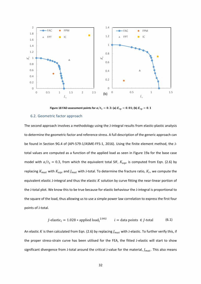
Figure 18 shows the influence of the loading condition on the acceptability of a defect using the FAD
approach for a sandwich pipe swage joint. The assessment points are displayed for a circumferential
crack with crack-to-thickness ratio, 𝑎𝑎 𝑡𝑡1⁄ = 0.3 and the influence of the filler resin stiffness is shown.
We see that the stiffness of the filler resin can alter the acceptability of an assessment point under
the perfect adhesion assumption for this approach applied based on LEFM. The crack and loading
conditions analogous to the points that lie within the failure assessment curve are deemed
acceptable, as they would not lead to unstable crack growth. As can be inferred, this approach is
better suited for brittle materials as it does not take into consideration the elastic-plastic behaviour
of the pipe material.
32
Figure 18 FAD assessment points for 𝒂𝒂 𝒕𝒕𝟏𝟏 = 𝟎𝟎.𝟑𝟑⁄ : (a) 𝑬𝑬𝒓𝒓𝒑𝒑 = 𝟎𝟎.𝟎𝟎𝟏𝟏; (b) 𝑬𝑬𝒓𝒓𝒑𝒑 = 𝟎𝟎.𝟏𝟏
6.2. Geometric factor approach
The second approach involves a methodology using the J-integral results from elastic-plastic analysis
to determine the geometric factor and reference stress. A full description of the generic approach can
be found in Section 9G.4 of (API-579-1/ASME-FFS-1, 2016). Using the finite element method, the J-
total values are computed as a function of the applied load as seen in Figure 19a for the base case
model with 𝑎𝑎 𝑡𝑡1⁄ = 0.3, from which the equivalent total SIF, 𝐾𝐾𝑒𝑒𝑒𝑒𝑒𝑒 is computed from Eqn. (2.6) by
replacing 𝐾𝐾𝑚𝑚𝑚𝑚𝑚𝑚 with 𝐾𝐾𝑒𝑒𝑒𝑒𝑒𝑒 and 𝐽𝐽𝑚𝑚𝑚𝑚𝑚𝑚 with J-total. To determine the fracture ratio, 𝐾𝐾𝑟𝑟, we compute the
equivalent elastic J-integral and thus the elastic 𝐾𝐾 solution by curve fitting the near-linear portion of
the J-total plot. We know this to be true because for elastic behaviour the J-integral is proportional to
the square of the load, thus allowing us to use a simple power law correlation to express the first four
points of J-total.
𝐽𝐽-elastic𝑖𝑖 = 1.028 ∗ applied loadi2.002 𝑖𝑖 = data points ∈ 𝐽𝐽-total
An elastic 𝐾𝐾 is then calculated from Eqn. (2.6) by replacing 𝐽𝐽𝑚𝑚𝑚𝑚𝑚𝑚 with J-elastic. To further verify this, if
the proper stress-strain curve has been utilised for the FEA, the fitted J-elastic will start to show
significant divergence from J-total around the critical J-value for the material, 𝐽𝐽𝑚𝑚𝑚𝑚𝑚𝑚. This also means
0
0.2
0.4
0.6
0.8
1
1.2
1.4
1.6
1.8
2
0 0.5 1 1.5 2 2.5
Kr
Lr
FAC FPM
FPT IC
0
0.2
0.4
0.6
0.8
1
1.2
1.4
0 0.5 1 1.5
Kr
Lr
FAC FPM
FPT IC
(b)
(6.1)

33
that, as plasticity increases at the crack front, the divergence increases, inferring that J-total is a
function of the load and crack dimension. The method specific fracture ratio 𝐾𝐾𝑟𝑟∗, is then expressed as
the ratio between the elastic 𝐾𝐾 and 𝐾𝐾𝑒𝑒𝑒𝑒𝑒𝑒 and plotted against the applied load as seen in Figure 19b.
We then derive the material specific 𝐾𝐾𝑟𝑟 value (similar to 𝐾𝐾𝑟𝑟 at 𝐿𝐿𝑟𝑟 = 1 from material specific FAC in (BS
7910, 2013) from the (API-579-1/ASME-FFS-1, 2016) equation 9G.3:
𝐾𝐾𝑟𝑟𝐿𝐿𝑟𝑟=1 = ��1 +
0.002𝐸𝐸𝜎𝜎𝑦𝑦
+ 0.5�1 +0.002𝐸𝐸𝜎𝜎𝑦𝑦
�−1
�
−1
Figure 19 (a) J-total, J-elastic for 𝒂𝒂 𝒕𝒕𝟏𝟏⁄ = 𝟎𝟎.𝟑𝟑 under axial loading (b) Nominal load at material specific 𝑲𝑲𝒓𝒓
The intersection of 𝐾𝐾𝑟𝑟𝐿𝐿𝑟𝑟=1 with 𝐾𝐾𝑟𝑟∗ gives us the nominal load 𝜎𝜎𝑛𝑛 unique to this joint configuration and
crack dimension from which we derive the geometric factor 𝐹𝐹𝑟𝑟𝑒𝑒𝑒𝑒 using:
𝐹𝐹𝑟𝑟𝑒𝑒𝑒𝑒 =𝜎𝜎𝑦𝑦𝜎𝜎𝑛𝑛
Furthermore, we see that the geometric factor is a function of the crack dimensions and allows us to
calculate the reference stress for any specific load 𝜎𝜎𝑑𝑑 applied to the sandwich pipe joint using:
𝜎𝜎𝑟𝑟𝑒𝑒𝑒𝑒 = 𝐹𝐹𝑟𝑟𝑒𝑒𝑒𝑒𝜎𝜎𝑑𝑑
0
50
100
150
200
0 100 200 300
J (KN
/m)
Axial load (MPa)
J-total
J-elastic
0
0.2
0.4
0.6
0.8
1
1.2
0 100 200 300
K r*
Axial load (MPa)
KrLr=1
σn
(a) (b)
(6.3)
(6.4)
(6.2)
34
The advantage of this approach is its capability to be used for a variety of structural geometries and
crack locations, even more so in scenarios where existing reference stress and stress intensity
solutions are not available (Thorwald and Vargas, 2017). Figure 20a shows the influence of the crack
to pipe thickness ratio (𝑎𝑎 𝑡𝑡1⁄ ) on 𝐹𝐹𝑟𝑟𝑒𝑒𝑒𝑒 for a circumferential swage weld toe crack in a sandwich joint
assembly. In contrast, for the loading cases, we can see that 𝐹𝐹𝑟𝑟𝑒𝑒𝑒𝑒 shows stronger dependence on 𝑎𝑎 𝑡𝑡1⁄
for isolated monotonic loads. The simulated installation case (a combination of monotonic load steps)
shows lesser dependence mainly due to the hydrostatic loading. This is because it is assumed that the
friction between the pipe and seabed is large enough to restrict lateral and longitudinal movement at
the touchdown point, which means the hydrostatic pressure acting on the joint assembly will induce
compressive stresses on the inner pipe. These stresses are further relieved by the axial stress induce
due to the pipe’s weight and bending stress at tensile side of the sagbend. It should be mentioned
here that the isolated load cases give a geometric factor at an equivalent stress value where we can
extract the nominal load for the lowest studied 𝑎𝑎 𝑡𝑡1⁄ value. For example, for the curvature control
load step (FPM case), we can see that an equivalent bending stress value of 322MPa needs to be
attained whereas an equivalent axial stress of 245MPa needs to be attained for the tension load case.
The influence of material plasticity on the acceptability of an assessment point is shown in Figure 20b
as contrasted with the failure assessment curve (BS 7910, 2013) from the elastic analysis. Four
different assessment points are considered at constant bending moment applied to the joint
assembly. It can be seen that if we consider plasticity in the development of the failure assessment
curve, the 𝑎𝑎 𝑡𝑡1⁄ = 0.63 assessment point would be deemed acceptable. In the absence of any code or
standard, that provides procedural guidance for the fracture toughness testing and fatigue crack
growth rate testing of the sandwich pipe swage joint geometry, the ECA via FE elastic-plastic analysis
provides the general assessment procedure.

35
Figure 20 (a) Influence of the crack depth/inner pipe thickness ratio on the geometric factor; (b) Influence of plasticity on the acceptability criteria for assessment points
7. Conclusions
Sandwich pipes have been shown to be a viable solution to both the thermal insulation and weight
requirement constraints for deepwater installation. To ensure these benefits, the integrity of the
sandwich pipe swage welds need to be preserved and this calls for, in most cases, bespoke solutions
due to the geometry and loading type. This also means that a certified non-destructive examination
procedure needs to be developed that adequately covers practical areas for sandwich pipe
utilisation.
This paper has focused on the engineering critical assessment of the swaged weld of a sandwich pipe
joint. It follows a fitness-for-purpose acceptance criteria based on FE fracture mechanics analysis, with
the main conclusions being:
• For a defect free model, the swaged weld was shown to be a stress raiser and the stress
distribution around the swage weld was visualized using finite element models. For the range
of elastic modulus ratios studied, results showed the weld toe to be the location of the
greatest stress discontinuity and thus the critical defect location under installation type
loading.
0
1
2
3
4
5
0.00 0.20 0.40 0.60 0.80
F ref
a/t1
FPT @245MPaFPM @322MPaIC @270MPa
0.16
0.31
0.470.63
0
0.2
0.4
0.6
0.8
1
1.2
0.0 0.5 1.0 1.5
Kr
Lr
FAC:BS 7910
FPM
FAC:J-integral
(a) (b)
36
• For elastic analysis, parametric studies showed that the swaged weld dimensions are critical
design variables that influence the stress distribution around the joint. The stress
concentration factor at the swaged weld toe has a direct proportional relationship to the weld
gap 𝑤𝑤𝑔𝑔 and weld-to-pipe elastic modulus ratio 𝐸𝐸𝑤𝑤𝑝𝑝 and an inverse relationship to the weld
length 𝑤𝑤𝑙𝑙 and thickness-to-radius ratio 𝑡𝑡1 𝑓𝑓1⁄ .
• A set of parametric correlations are derived from results of 12500 FE models to express the
relationship between the swage weld dimensions, elastic material properties and SCF for an
axial loading case with perfect adhesion between all layers. Another set of parametric
correlations were derived for the through thickness stress profile at the weld toe. Random
design sets of model parameters were used to check the accuracy of the fitted equations to
the FE models, with the largest error being 13.9% within the validity of the correlations.
• The FE fracture mechanics analysis is ideal for determining the acceptable defect size for the
swage weld. Reference stress solutions can be extracted by the direct stress linearization of
FEA results at the location of interest. The FE fracture mechanics analysis has the added
advantage over analytical solutions, in that it captures the direct influence of a stress raiser
(e.g high-low) on the stress distribution around the defect. It also captures how this
influence varies due to the proximity of the stress raiser and the defect dimensions.
• For the modelling of isotropic materials with the perfect adhesion assumption, the better
the load bearing properties of the annular materials, the lesser the stress state at constant
load, and the lesser the elastic stress intensity factor for a swaged weld toe defect. J-value
computation for elastic analysis is a directly proportional to the crack front stress-state
within the contour domain.
• For design against plastic collapse, the FE fracture mechanics assessment outlined in
(DNVGL-RP-F108, 2017) can be adopted for the swaged weld; with the aid of FEA to
accurately predict the reference stress due to maximum potential loading during installation
and a FAD to assess the maximum acceptable defect sizes. The methodology is also

37
applicable for elastic-plastic analysis, where it was shown that designing with plasticity
considerations (e.g. strain-based design) indeed has an influence on the acceptability of a
defect size. This sheds light to the conservative nature of brittle fracture design for materials
with significant ductility.
• For elastic-plastic fracture assessment, the FE fitness-for-service approach for components
with cracks outlined in (API-579-1/ASME-FFS-1, 2016) yields geometric factors for the
swaged weld geometry and load case which can is used to compute the reference stress
solution. The geometric factor for the swaged weld toe increases as a t1⁄ increases for all
potential load cases during installation.
A conservative form of assessment has been applied for the two approaches mainly because of the
weighty analysis involved in arriving at correlations for the unique swage joint. Further works are
encouraged especially in quantifying the influence of the core and filler properties on the fracture
mechanics inputs needed to carry out an engineering critical assessment for the joint. In addition, the
influence of the interlayer properties between the pipe/core and pipe/resin is unknown as all studies
were carried out assuming perfect adhesion. Although we know from theory that high welding
residual stress can exist in joints, and in-play, modify the reference stress and stress profile at the
crack tip, the effect of welding residual stress was not captured in this study. In addition, the study
only considers monotonic loads for an installation case and further works into fatigue loading are
highly recommended.
Acknowledgements
The authors would like to acknowledge the financial support of the University of Aberdeen, through
the Elphinstone PhD Studentship, and the support of the Maxwell computer cluster funded by the
University of Aberdeen.

38
References
ABAQUS 2014. ABAQUS User's and Theory Manuals. Version 6.14 ed.: Dassault.Systèmes. API-579-1/ASME-FFS-1 2016. Fitness-For-Service. Annex 9G, Section 9G-4, Finite Element Analysis of
Components with Cracks. Washington D.C 20005: API Publishing Services. API-RP-1111 2015. Design, Construction, Operation and Maintenance of Offshore Hydrocarbon
Pipelines (Limit State Design) 5th Edition. American Petroleum Institute: API Publishing Services.
ARJOMANDI, K. & TAHERI, F. 2011. A new look at the external pressure capacity of sandwich pipes. Marine Structures, 24, 23-42.
ARUN, S., SHERRY, A. H., SMITH, M. C. & SHEIKH, M. 2014. Finite Element Simulation of a Circumferential Through-Thickness Crack in a Cylinder. V003T03A086-C1 - Volume 3: Design and Analysis.
ASME BPVC-VIII-2 2015. Rules for Construction of Pressure Vessels Division 2-Alternative Rules. NY, USA: American Society of Mechanical Engineers, ASME.
BAI, Y. & Q., B. 2005. Limit-state based Strength Design. In: Y., B. & Q., B. (eds.) Subsea Pipelines and Risers. Oxford: Elsevier Science Ltd.
BAI, Y. & BAI, Q. 2005. Installation Design. In: Y, B. & Q, B. (eds.) Subsea Pipelines and Risers. Oxford: Elsevier Science Ltd.
BELL, R., CANADA CENTRE FOR MINERAL AND ENERGY, T. & CARLETON UNIVERSITY. FACULTY OF, E. 1985. Determination of Stress Intensity Factor for Weld Toe Defects, Phase II: Final Report, Carleton University, Faculty of Engineering.
BJERKE, S. L., SCULTORI, M. & WÄSTBERG, S. 2011. DNV’s Strain-based Fracture Assessment Approach for Pipeline Girth Welds. International Offshore and Polar Engineering Conference. Maui, Hawaii, USA: ISOPE.
BS 7910 2013. Guide to Methods for Assessing the Acceptability of Flaws in Metallic Structures. Assessment for Fatigue;Assessment for Fracture Resistance British Standards Publication.
DASSAULT SYSTÈMES 2012. Modeling Cracks & Fracture Analysis, MA, USA, Dassault Systèmes Americas Corp.
DIXON, M., JACKSON, D. & EL CHAYEB, A. 2003. Deepwater Installation Techniques for Pipe-in-Pipe Systems Incorporating Plastic Strains. Offshore Technology Conference. Houston, Texas: Offshore Technology Conference.
DNV-OS-F101 2007. Submarine pipeline systems. Appendix A: Structural Integrity of Pipeline Girth Welds in Offshore Pipelines Det Norske Veritas AS.
DNV-RP-A203 2011. Qualification of New Technology. Norway: DNV, Det Norske Veritas AS. DNVGL-RP-F108 2017. Assessment of flaws in pipeline and riser girth welds. Use of Finite Element
Fracture Mechanics Analyses to Assess Maximum Allowable Flaw Sizes. DNV GL AS. IRWIN, G. R. 1961. Plastic zone near a crack and fracture toughness. In: Mechanical and metallurgical
behavior of sheet materials. 7th Sagamore Ordnance Materials Research, 63-78. JONES, R. L., GEERTSEN, C., BOOTH, P., MAIR, J. A., SRISKANDARAJAH, T. & RAO, V. 2013. Pipe-in-
Pipe Swaged Field Joint for Reel Lay. Offshore Technology Conference. Houston, Texas, USA: OTC.
39
KIBEY, S., WANG, X., MINNAAR, K., MACIA, M. L., FAIRCHILD, D. P., KAN, W. C., FORD, S. J. & NEWBURY, B. 2010. Tensile Strain Capacity Equations for Strain-Based Design of Welded Pipelines. 355-363
C1 - 2010 8th International Pipeline Conference, Volume 4. KYRIAKIDES, S. & CORONA, E. 2007. 2 - Offshore Facilities and Pipeline Installation Methods. In:
CORONA, S. K. (ed.) Mechanics of Offshore Pipelines. Oxford: Elsevier Science Ltd. MALLIK, A., ATIN, C., WANG, J., DELEYE, X. & LEGRAS, J.-L. 2013. Control of the Integrity of Swaged
Weld on Insulated Pipe-in-Pipe. Offshore Technology Conference. Houston, Texas, USA: OTC. MORGAN, M. R. & LEE, M. M. K. 1998. Parametric equations for distributions of stress concentration
factors in tubular K-joints under out-of-plane moment loading. International Journal of Fatigue, 20, 449-461.
ONYEGIRI, I. & KASHTALYAN, M. 2017. Finite element analysis of a sandwich pipe joint. Ocean Engineering, 146, 363-374.
O�STBY, E. 2005. Fracture Control — Offshore Pipelines: New Strain-Based Fracture Mechanics Equations Including the Effects of Biaxial Loading, Mismatch, and Misalignment. 649-658. C1 - 24th International Conference on Offshore Mechanics and Arctic Engineering: Volume 3.
PISARSKI, H. 2011. Assessment of Flaws in Pipe Girth Welds. CBMM-TMS International Conference on Welding of High Strength Pipeline Steels. Araxá, Brasil.
PISARSKI, H., XU, G. & SMITH , S. 2006. Fracture mechanics assessment of flaws in pipeline girth welds. International Seminar on Application of High Strength Line Pipe And Integrity Assessment of Pipeline. Xi'an, China: HSLP-IAP.
SIGMAPLOT 2014. Version 13 ed. San Jose, CA, USA: Systat Software Inc. SUN, C. T. & JIN, Z. H. 2012. Chapter 3 - The Elastic Stress Field around a Crack Tip. In: SUN, C. T. &
JIN, Z. H. (eds.) Fracture Mechanics. Boston: Academic Press. THORWALD, G. & VARGAS, P. 2017. Cylinder Axial Crack Reference Stress Comparison Using Elastic-
Plastic FEA 3D Crack Mesh J-Integral Values. V03BT03A031-C1 - Volume 3B: Design and Analysis.
VITALI, L., BRUSCHI, R., MORK, K. J., LEVOLD, E. & VERLEY, R. 1999. Hotpipe Project: Capacity of Pipes Subject to Internal Pressure, Axial Force And Bending Moment. International Society of Offshore and Polar Engineers.
YOO, A. B., JETTE, M. A. & GRONDONA, M. SLURM: Simple Linux Utility for Resource Management. In: FEITELSON, D., RUDOLPH, L. & SCHWIEGELSHOHN, U., eds. Job Scheduling Strategies for Parallel Processing, 2003// 2003 Berlin, Heidelberg. Springer Berlin Heidelberg, 44-60.
ZEHNDER, A. T. 2012. Fracture Mechanics, Dordrecht, Netherlands, Springer. ZHU, X.-K. & JOYCE, J. A. 2012. Review of fracture toughness (G, K, J, CTOD, CTOA) testing and
standardization. Engineering Fracture Mechanics, 85, 1-46.