engineering design 2
TRANSCRIPT

chapter 11: Mater ia ls Select ion 501
11
With the removal of lead compounds from gasoline has come an easing of the high-
temperature corrosion problems that cause burning, but a new problem has arisen. The
combustion products of lead-free gasoline lack the lubricity characteristics of those of
fuels that contain lead. As a result, the wear rates at the valve seating surfaces have in-
creased signiI cantly. The solution has been to harden the cast-iron cylinder head to im-
prove its wear resistance or install a wear-resistant insert. Unless one or the other is done,
the wear debris will weld to the valve seat and cause extensive damage. With increased
use of hard-alloy inserts, it is becoming more common to hard-face the valve seat with a
Stellite alloy.
E X A M P L E 1 1 . 7 Material Substitution
This design example illustrates the common problem of substituting a new material for
one that has been used for some time. It illustrates that material substitution should not be
undertaken unless appropriate design changes are made. Also, it illustrates some of the
practical steps that must be taken to ensure that the new material and design will perform
adequately in service.
Aluminum alloys have been substituted for gray cast iron 27 in the external supporting
parts of integral-horsepower induction motors (Fig. 11.13). The change in materials was
brought about by increasing cost and decreasing availability of gray-iron castings. There
has been a substantial reduction in gray-iron foundries, partly because of increased costs
resulting from the more stringent environmental pollution and safety regulations imposed
in recent years by governmental agencies. The availability of aluminum castings has in-
creased owing to new technology to increase the quality of aluminum castings. Also, with
aluminum castings there are fewer problems in operating an aluminum foundry, which
operates at a much lower temperature than those required for cast iron.
There are a variety of aluminum casting alloys. 28 Among the service requirements
for this application, strength and corrosion resistance were paramount. The need to pro-
vide good corrosion resistance to water vapor introduced the requirement to limit the
27. T. C . Johnson and W. R . Morton , IEEE Conference Record 76CH1 109-8-IA, Paper PCI-76-14, Gen-
eral Electric Company Report GER-3007 .
28. Metals Handbook: Desk Edition , 2d ed., “Aluminum Foundry Products,” ASM International , 1998 .
pp. 484–96 .
FIGURE 11.14 Horizontal aluminum alloy motor.
(Courtesy of General Electric Company.)
die37039_ch11.indd 501 2/25/08 6:58:30 PM

502 engineering design
11
copper content to an amount just sufI cient to achieve the necessary strength. Actual al-
loy selection was dependent on the manufacturing processes used to make the part. That
in turn depended chieh y (see Chap. 13) on the shape and the required quantity of parts.
Table 11.9 gives details on the alloys selected for this application.
Since the motor frame and end-shield assemblies have been made successfully from
gray cast iron for many years, a comparison of the mechanical properties of the alumi-
num alloys with cast iron is important (Table 11.10).
The strength properties for the aluminum alloys are approximately equal to or exceed
those of gray cast iron. If the slightly lower yield strength for alloy 356 cannot be tolerated,
it can be increased appreciably by a solution heat treatment and aging (T6 condition) at a
slight penalty in cost and corrosion resistance. Since the yield and shear strength of the
aluminum alloys and gray cast iron are about equal, the section thickness of aluminum to
withstand the loads would be the same. However, since the density of aluminum is about
one-third that of cast iron, there will be appreciable weight saving. The complete alumi-
num motor frame is 40 percent lighter than the equivalent cast iron design. Moreover, gray
cast iron is essentially a brittle material, whereas the cast-aluminum alloys have enough
malleability that bent cooling I ns can be straightened without breaking them.
The aluminum alloys are inferior to cast iron in compressive strength. In aluminum,
as with most alloys, the compressive strength is about equal to the tensile strength, but
in cast iron the compressive strength is several times the tensile strength. That becomes
important at bearing supports, where, if the load is unbalanced, the bearing can put an
appreciable compressive load on the material surrounding and supporting it. That leads to
excessive wear with an aluminum alloy end shield.
TABLE 11.9
Aluminum Alloys Used in External Parts of Motors
Composition
Part Alloy Cu Mg Si Casting Process
Motor frame 356 0.2 max 0.35 7.0 Permanent mold
End shields 356 0.2 max 0.35 7.0 Permanent mold
Fan casing 356 0.2 max 0.35 7.0 Permanent mold
Conduit box 360 0.6 max 0.50 9.5 Die casting
TABLE 11.10
Comparison of Typical Mechanical Properties
MaterialYield
Strength, ksiUltimate Tensile
Strength, ksiShear
Strength, ksiElongation in 2 in, percent
Gray cast iron 18 22 20 0.5
Alloy 356 (as cast) 15 26 18 3.5
Alloy 360 (as cast) 25 26 45 3.5
Alloy 356-T61 28 38 5
(solution heat-treated
and artiI cially aged)
die37039_ch11.indd 502 2/25/08 6:58:32 PM

chapter 11: Mater ia ls Select ion 503
11
To minimize the problem, a steel insert ring is set into the aluminum alloy end shield
when it is cast. The design eliminates any clearance I t between the steel and aluminum,
and the steel insert resists wear from the motion of the bearing just as the cast iron always
did. The greater ease of casting aluminum alloys permits the use of cooling I ns thinner
and in greater number than in cast iron. Also, the thermal conductivity of aluminum is
about three times greater than that of cast iron. Those factors result in more uniform
temperature throughout the motor, and this results in longer life and higher reliability.
Because of the higher thermal conductivity and larger surface area of cooling I ns, less
cooling air is needed. With the air requirements thus reduced, a smaller fan can be used,
also resulting in a small reduction of noise.
The coefI cient of expansion of aluminum is greater than that of cast iron, and that
makes it easier to ensure a tight I t of motor frame to the core. Only a moderate tempera-
ture rise is needed to expand the aluminum frame sufI ciently to insert the core, and on
cooling the frame contracts to make a tight bond with the core. That results in a tighter
I t between the aluminum frame and the core and better heat transfer to the cooling I ns.
Complete design calculations need to be made when aluminum is substituted for cast iron
to be sure that clearances and interferences from thermal expansion are proper.
Since a motor design that had many years of successful service was being changed
in a major way, it was important to subject the redesigned motor to a variety of simulated
service tests. The following were used:
Vibration test Navy shock test (MIL-Std-901) Salt fog test (ASTM B 1 17-57T) Axial and transverse strength of end shield Strength of integral cast lifting lugs Tests for galvanic corrosion between aluminum alloy parts and steel bolts
This example illustrates the importance of considering design and manufacturing
together in a material substitution situation.
11.11 RECYCLING AND MATERIALS SELECTION
The heightened public awareness of environmental issues has resulted in signiI cant legislation and regulation that provide new constraints on design. For example, in Germany a law requires manufacturers to take back all packaging used in the trans-port and distribution of a product, and in the Netherlands old or broken appliances must be returned to the manufacturer for recycling. Traditionally the recycling and re-use of materials was dictated completely by economics. Those materials like steel, and more recently aluminum cans, that can be collected and reprocessed at a proI t were recycled. However, with widespread popular support for improving the environment, other beneI ts of recycling are being recognized.
The complete life cycle of a material is shown in Fig. 1.6. The materials cycle starts with the mining of a mineral or the drilling for oil or the harvesting of an agri-cultural I ber like cotton. These raw materials must be processed to reI ne or extract bulk material (e.g., a steel ingot) that is further processed into a I nished engineering
●
●
●
●
●
●
die37039_ch11.indd 503 2/25/08 6:58:32 PM

504 engineering design
11
material (e.g., a steel sheet). At this stage an engineer designs a product that is manu-factured from the material, and the product is put into useful service. Eventually the product wears out or is made obsolete because a better product comes on the market. At this stage our tendency has been to junk the product and dispose of it in some way, like a landI ll, that eventually returns the material to the earth. However, society is more and more mindful of the dangers to the environment of such haphazard prac-tices. As a result, more emphasis is being placed on recycling of the material directly back into the materials cycle.
11.11.1 BeneG ts from Recycling
The obvious beneI ts of materials recycling are the contribution to the supply of ma-terials, with corresponding reduction in the consumption of natural resources, and the reduction in the volume of solid waste. Moreover, recycling contributes to environ-mental improvement through the amount of energy saved by producing the material from recycled (secondary) material rather than primary sources (ore or chemical feed-stock). Recycled aluminum requires only 5 percent of the energy required to produce it from the ore. Between 10 and 15 percent of the total energy used in the United States is devoted to the production of steel, aluminum, plastics, or paper. Since most of this is generated from fossil fuels, the saving from carbon dioxide and particulate emissions due to recycling is appreciable.
Recycling of materials also directly reduces pollution. For example, the use of steel scrap in making steel bypasses the blast furnace at a considerable economic ben-eI t. Bypassing the blast furnace in processing eliminates the pollution associated with it, particularly since there is no longer a need for the production of coke, which is an essential ingredient for blast furnace smelting.
An alternative to recycling is remanufacturing . Instead of the product being dis-assembled for recycling, remanufacturing restores it to near new condition by cleaning and replacement of worn parts. We have long been familiar with rebuilt automotive parts, like alternators and carburetors, but now remanufacture has moved to appli-ances such as copiers and printers, and to large engineered products like diesel en-gines and construction equipment.
11.11.2 Steps in Recycling
The steps in recycling a material are (1) collection and transport, (2) separation, and (3) identiI cation and sorting. 29
Collection and Transport
Collection for recycling is determined by the location in the material cycle where the discarded material is found. Home scrap is residual material from primary
29. “Design for Recycling and Life Cycle Analysis,” Metals Handbook, Desk Edition , 2d ed., ASM In-
ternational, Materials Park, OH , 1998 , pp. 1196–99 .
die37039_ch11.indd 504 2/25/08 6:58:32 PM

chapter 11: Mater ia ls Select ion 505
11
material production, like cropped material from ingots or sheared edges from plates, which can be returned directly to the production process. Essentially all home scrap is recycled. Prompt industrial scrap or new scrap is that generated during the manufac-ture of products, for example, compressed bundles of lathe turnings or stamping dis-card from sheets. This is sold directly in large quantities by the manufacturing plant to the material producer. Old scrap is scrap generated from a product which has com-pleted its useful life, such as, a scrapped automobile or refrigerator. These products are collected and processed in a scrap yard and sold to material producers. The collec-tion of recycled material from consumers can be a more difI cult proposition because it is widely distributed. Materials can be economically recycled only if an effective collection system can be established, as with aluminum cans. Collection methods in-clude curbside pickup, buy-back centers (for some containers), and resource recovery centers where solid waste is sorted for recyclables and the waste is burned for energy.
Separation
Separation of economically proI table recyclable material from scrap typically follows one of two paths. In the I rst, selective dismantling takes place. Toxic mate-rials like engine oil or lead batteries are removed I rst and given special treatment. High-value materials like gold and copper are removed and segregated appropriately. Dismantling leads naturally to sorting of materials into like categories. The second separation route is shredding, in which the product is subjected to multiple high-energy impacts to batter it into small, irregular pieces. For example, automobile hulks are routinely processed by shredding. Shredding creates a material form that assists in separation. Ferrous material can be removed with large magnets, leaving behind a debris that must be disposed off, sometimes by incineration.
IdentiG cation and Sorting
The economic value of recycling is largely dependent on the degree to which ma-terials can be identiI ed and sorted into categories. Material that has been produced by recycling is generally called secondary material . The addition of secondary ma-terial to “virgin material” in melting or molding can degrade the properties of the resultant material if the chemical composition of the secondary material is not care-fully controlled. Generally this is less of a problem with metals than with plastics. In metallic alloys, there is generally a limit on “tramp elements” that inh uence critical mechanical properties or workability or castability. Some alloys are restricted to the use of virgin material. There also are aluminum casting alloys that have been speciI -cally designed to be tolerant of large amounts of secondary metal. In steel, more than 0.20% copper or 0.06% tin cause cracking in hot working. As more and more steel is recycled through scrap, there is concern about a buildup in these critical elements. Thus, the price of metal scrap depends on its freedom from tramp elements, which is determined by the effectiveness of the identiI cation and separation process.
Degradation of plastics from secondary materials is more critical than that of metals, since it is often difI cult to ensure that different types of polymers were not mixed together. Only thermoplastic polymers can be recycled. Thermosets, which are degraded by high temperature, cannot be recycled. Often, recycled material is used for a less critical application than its original use. There is an intensive effort to improve
die37039_ch11.indd 505 2/25/08 6:58:33 PM
506 engineering design
11
the recycling of plastics, and it is claimed that under the best of conditions engineered plastics can be recycled three or four times without losing more than 5 to 10 percent of their original strength. Other materials that may not be economically recycled are zinc-coated steel (galvanized), ceramic materials (except glass), and parts with glued identiI cation labels made from a different material than the part. Composite mate-rials consisting of mixtures of glass and polymer represent an extreme problem in recycling.
Metals are identiI ed by chemical spot testing or by magnetic or h uorescence anal-ysis. Different grades of steel can be identiI ed by looking at the sparks produced by a grinding wheel. IdentiI cation of plastics is more difI cult. Fortunately, most manufac-turers have adopted the practice of molding or casting a standard Society for the Plas-tic Industry identiI cation symbol into the surface of plastic parts. This consists of a triangle having a number in the middle to identify the type of plastic. 30 Much effort is being given to developing devices that can identify the chemical composition of plastic parts at rates of more than 100 pieces per second, much like a bar-code scanner.
Ferrous metals are separated from other materials by magnetic separation. For nonferrous metals, plastics, and glass, separation is achieved by using such methods as vibratory sieving, air classiI cation, and wet h otation. However, much hand sorting is used.
After sorting, the recycled material is sold to a secondary materials producer. Metals are remelted into ingots; plastics are ground and processed into pellets. These are then introduced into the materials stream by selling the recycled material to part manufacturers.
11.11.3 Design for Recycling
There are several steps that the designer can take to enhance the recyclability of a product.
Make it easier to disassemble the product, and thus enhance the yield of the separa-tion step.
Minimize the number of different materials in the product to simplify the identiI -cation and sorting issue.
Choose materials that are compatible and do not require separation before recycling.
Identify the material that the part is made from right on the part. Use the identiI ca-tion symbols for plastics.
These guidelines can lead to contradictions that require serious trade-offs. Minimiz-ing the number of materials in the original product may require a compromise in performance from the use of a material with less-than-optimum properties. Heavily galvanized steel can lead to unacceptable zinc buildup in steel scrap, yet the galvanized
●
●
●
●
30 . The following is the identiI cation scheme: 1, polyethylene; 2, high-density polyethylene; 3, vinyl;
4, low-density polyethylene; 5, polypropylene; 6, polystyrene; 7, other.
die37039_ch11.indd 506 2/25/08 6:58:33 PM

chapter 11: Mater ia ls Select ion 507
11
undercoat has greatly reduced corrosion on automobile bodies. A clad metal sheet or chromium-plated metal provides the desired attractive surface at a reasonable cost, yet it cannot be readily recycled. In the past, decisions of this type would be made exclusively on the basis of cost. Today, we are moving toward a situation where the customer may be willing to pay extra for a recyclable design, or the recyclable design may be mandated by government regulations. Decision making on recycling requires input from top management in consultation with material recycling experts.
E X A M P L E 1 1 . 8
Terne-coated steel (8 percent tin-lead coating) has been the traditional material selection
for automotive gas tanks. 31 A number of federal laws have mandated radical changes in au-
tomotive design. Chief among these is the act which mandates the Corporate Average Fuel
Economy, which creates an incentive for weight reduction to increase gas mileage. The
Alternative Motor Fuels Act of 1988 and the Clear Air Act Amendments of 1990 created
a need to prepare for the wider use of alternative-fuel vehicles to reduce oil imports and
to increase the use of U.S. sourced renewable fuels such as ethanol. Tests have shown that
neither painted nor bare terne-coated steel will resist the corrosive effects of alcohol for
the 10-year expected life of the fuel tank. In addition, the EPA has introduced fuel-perme-
ation standards that challenge the designs and materials used in automotive fuel tanks.
In the selection of a material for an automotive fuel tank, the following factors
are most important: manufacturability/cost/weight/corrosion resistance/permeability
resistance/ recyclability. Another critical factor is safety and the ability to meet crash
requirements.
Two new competing materials have emerged to replace terne steel: electrocoated
zinc-nickel steel sheet and high-density polyethylene (HDPE). The steel sheet is painted
on both sides with an aluminum-rich epoxy. The epoxy is needed to provide exterior pro-
tection from road-induced corrosion. Stainless steel performs admirably for this applica-
tion but at nearly I ve times the cost. HDPE is readily formed by blow-molding into the
necessary shape, and if has long-term structural stability, but it will not meet the perme-
ability requirement. Two approaches have been used to overcome this problem. The I rst
is multilayer technology, in which an inner layer of HDPE is adhesively joined to a barrier
layer of polyamide. The second approach is a barrier to permeability that involves treating
the HDPE with h uorine.
The I rst step in arriving at a material selection decision is to make a competitive
analysis, laying out the advantages and disadvantages of each candidate.
Steel
Terne-coated steel Advantages: low cost at high volumes, modest material cost, meets perme-
ability requirement Disadvantages: shape h exibility, poor corrosion protection from alcohol fu-
els, lead-containing coating gives problems with recycling or disposal Electrocoated Zn-Ni steel
Advantages: low cost at high volumes, effective corrosion protection, mate-rial cost, meets permeability requirement
31. P. J . Alvarado , “Steel vs. Plastics: The Competition for Light-Vehicle Fuel Tanks,” JOM, July 1996 ,
pp. 22–25 .
die37039_ch11.indd 507 2/25/08 6:58:33 PM

508 engineering design
11
Disadvantages: weldability, shape h exibility Stainless steel
Advantages: high corrosion resistance, recyclable, meets permeability re-quirements
Disadvantages: cost at all volumes, formability, weldability
Plastics
HDPE (high-density polyethylene) Advantages: shape h exibility, low tooling costs at low volumes, weight, cor-
rosion resistance Disadvantages: high tooling costs at high volumes, high material cost, does
not meet permeability and recyclability requirements Multilayer and barrier HDPE
Advantages: same as HDPE plus meets permeability requirement Disadvantages: higher tooling costs at high volume, higher material cost,
hard to recycle
The next step would be to use one of the matrix methods discussed in Sec. 11.9 to arrive
at the decision. Two of the Big Three automobile producers are changing to some variant
of the Zn-Ni coated steel. The other is going with HDPE fuel tanks. The fact that there is
not a clear superior choice demonstrates the complexity of selection decisions in the mod-
ern day when there often are so many competing issues.
11.11.4 Material Selection for Eco-attributes
The material performance index developed by Ashby (Sec. 11.8) can be extended to consider the environmental attributes of the material. 32 The following stages of the materials cycle must be considered: (1) material production, (2) product manufacture, (3) product use, and (4) product disposal.
Energy and Emissions Associated with Material Production
The greatest amount of environmental damage is done in producing a material. Most of the energy used in this process is obtained from fossil fuels: oil, gas, and coal. In many cases the fuel is part of the production process, in other cases it is I rst converted to electricity that is used in production. The pollution produced during ma-terial production takes the form of undesirable gas emissions, chieh y CO 2 , NO x , SO x , and CH 4 . For each kilogram of aluminum produced from fossil fuels there is created12 kg of CO 2 , 40 g of NO x , and 90 g of SO x . Also, individual processes may create toxic wastes and particulates that should be treated at the production site.
The fossil-fuel energy required to make one kilogram of material is called its pro-
duction energy. Table 11.11 lists some typical values of production energy, H p, as well as data on the production of CO 2 per kg of material produced.
32. M. F . Ashby , op. cit, Chap. 16.
die37039_ch11.indd 508 2/25/08 6:58:34 PM

chapter 11: Mater ia ls Select ion 509
11
Energy and Emissions Associated with Product Manufacture
The energy involved in manufacturing the product is at least an order of magnitude smaller than that required for producing the material. The energy for metal defor-mation processes like rolling or forging are typically in the range 0.01 to 1 MJ/kg. Polymer molding processes are 1 to 4 MJ/kg, while metal casting processes are 0.4 to 4 MJ/kg. While saving energy in manufacturing is important, of greater con-cern ecologically is eliminating any toxic wastes and polluted discharges created in manufacturing.
Energy Associated with Product Use
The energy consumed in product use is determined by the mechanical, thermal, and electrical efI ciencies achieved by the design of the product. Fuel efI ciency in a motor vehicle is achieved chieh y by reducing the mass of the vehicle, along with im-proving mechanical efI ciency of the transmission and minimizing aerodynamic losses.
Energy and Environmental Issues in Product Disposal
It is important to realize that some of the energy used in producing a material is stored in the material and can be reused in the recycling or disposal process. Wood and paper products can be burned in an incinerator and energy recovered. While some
TABLE 11.11
Values for Production Energy and Amount of CO 2 Produced
MaterialProduction Energy ( H p )
MJ/kgCO 2 Burden, [CO 2 ] kg/kg
Low-carbon steels 22.4 – 24.8 1.9 – 2.1
Stainless steels 77.2 – 80.3 4.8 – 5.4
Aluminum alloys 184 – 203 11.6 – 12.8
Copper alloys 63.0 – 69.7 3.9 – 4.4
Titanium alloys 885 – 945 41.7 – 59.5
Borosilicate glass 23.8 – 26.3 1.3 – 1.4
Porous brick 1.9 – 2.1 0.14 – 0.16
CFRP composites 259 – 286 21 – 23
PVC 63.5 – 70.2 1.85 – 2.04
Polyethylene (PE) 76.9 – 85 1.95 – 2.16
Nylons (PA) 102 – 113 4.0 – 4.41
From M.F . Ashby , Materials Selection in Mechanical Design, 3d ed. (Used
with permission of Butterworth-Heinemann.)
die37039_ch11.indd 509 2/25/08 6:58:34 PM

510 engineering design
11
energy is required for recycling, it is much less than H p . Recycled aluminum requires much less energy to melt it than is required to extract it from its ore.
Important information to know when selecting a material is:
Is there an economically viable recycling market for the material? This can be de-termined by checking websites for recycled materials, and by the fraction of the market for the material that is made from recycled materials.
It is important to know how readily the material can be added to virgin material without deleterious effects on properties. This is true recycling. Some materials can only be recycled into lower-grade materials.
Some materials can be disposed of by biodegradation in landI lls, while the bulk of materials that are not recycled go into landI lls. However, some materials like lead, cadmium, and some of the heavy metals are toxic, especially in I nely divided form, and must be disposed of by methods used for hazardous materials.
Material Performance Indices
Some of these environmental issues can be readily incorporated into the material performance index, Sec. 11.8. Suppose we wanted to select a material with minimum production energy to provide a given stiffness to a beam. We know from Sec. 11.8 that the minimum mass beam would be given by the largest value of M 5 E 1/2 /r from among the candidate materials. To also accommodate production energy in this deci-sion the material performance index would be written as
ME
Hp
=1 2/
ρ (11.13)
and to select a material with minimum CO 2 production for a beam of given bending strength
Mf
=[ ]
σ
ρ
2 3/
CO2 (11.14)
Production energy, H p , or CO 2 produced in smelting the material could be included in any of the material performance indices listed in Table 11.6. These terms are placed in the denominator because convention requires that high values of M determine the material selection.
11.12 SUMMARY
This chapter has shown that there are no magic formulas for materials selection. Rather, the solution of a materials selection problem is every bit as challenging as any other aspect of the design process and follows the same general approach of prob-
●
●
●
die37039_ch11.indd 510 2/25/08 6:58:34 PM

chapter 11: Mater ia ls Select ion 511
11
lem solving. Successful materials selection depends on the answers to the following questions.
Have performance requirements and service environments been properly and com-pletely deI ned? Is there a good match between the performance requirements and the material properties used in evaluating the candidate materials? Has the material’s properties and their modiI cation by subsequent manufacturing processes been fully considered? Is the material available in the shapes and conI gurations required and at an ac-ceptable price?
The steps in materials selection are:
DeI ne the functions that the design must perform and translate these into required materials properties, and to business factors such as cost and availability. DeI ne the manufacturing parameters such as number of parts required, size and complexity of the part, tolerances, quality level, and fabricability of the material. Compare the needed properties and process parameters with a large materials da-tabase to select a few materials that look promising for the application. Use several screening properties to identify the candidate materials. Investigate the candidate materials in greater detail, particularly in terms of trade-offs in performance, cost, and fabricability. Make a I nal selection of material. Develop design data and a design speciI cation.
Materials selection can never be totally separated from the consideration of how the part will be manufactured. This large topic is covered in Chap. 12. The Ashby charts are very useful for screening a wide number of materials at the conceptual design stage, and should be employed with materials performance indices. Computer screen-ing of materials databases is widely employed in embodiment design. Many of the evaluation methods that were introduced in Chap. 7 are readily applied to narrowing down the materials selection. The Pugh selection method and weighted decision ma-trix are most applicable. Failure analysis data (see Chap. 13) are an important input to materials selection when a design is modiI ed. The value analysis technique has broad implications in design, but it is especially useful for materials selection when a design review on a new product is being conducted or an existing product is being redesigned. Life-cycle issues should always be considered, especially those having to do with recycling and disposal of materials.
1.
2.
3.
4.
1.
2.
3.
4.
5.
NEW TERMS AND CONCEPTS
Anisotropic property Defect structure Scaled property
ASTM Go-no go material property Secondary material
Composite material Material performance index Structure-sensitive property
Crystal structure Polymer Thermoplastic material
Damping capacity Recycling Weighted property index
die37039_ch11.indd 511 2/25/08 6:58:35 PM

512 engineering design
11
BIBLIOGRAPHY
Ashby , M. F .: “Materials Selection in Mechanical Design,” 3d ed., Elsevier, Butterworth-
Heinemann, Oxford, UK , 2005 .
“ ASM Handbook,” vol. 20, “Materials Selection and Design,” ASM International, Materials
Park, OH , 1997 .
Budinski , K. G .: “ Engineering Materials: Properties and Selection,” 7th ed., Prentice Hall,
Upper Saddle River, NJ , 2002 .
Charles , J. A ., F. A. A . Crane , and J. A. G . Furness : “ Selection and Use of Engineering Materi-
als,” 3d ed., Butterworth Heinemann, Boston , 1997 .
Farag , M. M .: “ Materials Selection for Engineering Design, ” Prentice-Hall, London , 1997 .
Kern , R. F ., and M. E . Suess : “ Steel Selection, ” John Wiley, New York , 1979 .
Lewis , G .: “ Selection of Engineering Materials, ” Prentice-Hall, Englewood Cliffs, NJ , 1990 .
Mangonon , P. L .: “The Principles of Materials Selection for Engineering Design, ” Prentice-
Hall, Upper Saddle River, NJ , 1999 .
PROBLEMS AND EXERCISES
11.1 Think about why books are printed on paper. Suggest a number of alternative materi-
als that could be used. Under what conditions (costs, availability, etc.) would the alter-
native materials be most attractive?
11.2 Consider a soft drink can as a materials system. List all the components in the system
and consider alternative materials for each component.
11.3 Which material property would you select as a guide in material selection if the chief
performance characteristic of the component was: (a) strength in bending; (b) resis-
tance to twisting; (c) the ability of a sheet material to be stretched into a complex cur-
vature; (d) ability to resist fracture from cracks at low temperatures; (e) ability to resist
shattering if dropped on the h oor; (f) ability to resist alternating cycles of rapid heating
and cooling.
11.4 Rank-order the following materials for use as an automobile radiator: copper, stainless
steel, brass, aluminum, ABS, galvanized steel.
11.5 Select a tool material for thread-rolling mild-steel bolts. In your analysis of the prob-
lem you should consider the following points: (1) functional requirements of a good
tool material, (2) critical properties of a good tool material, (3) screening process for
candidate materials, and (4) selection process.
11.6 Table 11.3 gives a range of tensile properties for aluminum alloy 6061. Look up infor-
mation about this alloy and write a brief report about what processing steps are used
to achieve these properties. Include a brief discussion of the structural changes in the
material that are responsible for the change in tensile properties.
die37039_ch11.indd 512 2/25/08 6:58:35 PM

chapter 11: Mater ia ls Select ion 513
11
11.7 Determine the material performance index for a light, stiff beam. The beam is simply
supported with a concentrated load at midlength.
11.8 Determine the material performance indices for a connecting rod in a high-
performance engine for a racing car. The most likely failure modes are fatigue failure
and buckling at the critical section, where the thickness is b and the width is w. Use
the CES software to identify the most likely candidates in a material selection at the
conceptual design stage.
11.9 Use the information in Example 11.10 to construct a Pugh concept selection matrix to
aid in deciding which material to select.
11.10 Two materials are being considered for an application in which electrical conductivity
is important.
Material Working Strength MN/m 2 Electrical Conductance %
A 500 50
B 1000 40
The weighting factor on strength is 3 and 10 for conductance. Which material is pre-
ferred based on the weighted property index?
11.11 An aircraft windshield is rated according to the following material characteristics. The
weighting factors are shown in parentheses.
Resistance to shattering (10) The candidate materials are:
Fabricability (2)
Weight (8) A plate glass
Scratch resistance (9) B PMMA
Thermal expansion (5) C tempered glass
D a special polymer laminate
The properties are evaluated by a panel of technical experts, and they are expressed as
percentages of maximum achievable values.
Candidate Material
Property A B C D
Resistance to shattering 0 100 90 90
Fabricability 50 100 10 30
Weight 45 100 45 90
Scratch resistance 100 5 100 90
Thermal expansion 100 10 100 30
Use the weighted property index to select the best material.
11.12 A cantilever beam is loaded with force P at its free end to produce a deh ection d 5
PL 3 /3 EI . The beam has a circular cross section, I 5 π r 4 /4. Develop a I gure of merit for
die37039_ch11.indd 513 2/25/08 6:58:35 PM

514 engineering design
11
selecting a material that minimizes the weight of a beam for a given stiffness ( P /d).
By using the following material properties, select the best material (a) on the basis of
performance and (b) on the basis of cost and performance.
E
Material GNm 2 ksi R 1 Mgm 3 Approx. Cost, $/ton (1980)
Steel 200 29 x 10 3 7.8 450
Wood 9–16 1.7 x 10 3 0.4–0.8 450
Concrete 50 7.3 x 10 3 2.4–2.8 300
Aluminum 69 10 x 10 3 2.7 2,000
Carbon-I ber-
reinforced plastic
(CFRP)
70–200 15 x 10 3 1.5–1.6 200,000
11.13 Select the most economical steel plate to construct a spherical pressure vessel in which
to store gaseous nitrogen at a design pressure of 100 psi at ambient weather conditions
down to a minimum of 220°F. The pressure vessel has a radius of 138 in. Your selec-
tion should be based on the steels listed in the following table and expressed in terms
of cost per square foot of material. Use a value of 489 lb/ft 3 for the density of steel.
die37039_ch11.indd 514 2/25/08 6:58:36 PM

515
12
DESIGN WITH MATERIALS
12.1INTRODUCTION
This chapter deals with topics of material performance that are not usually covered in courses in strength of materials or machine design, but with which the mechanical designer needs to be familiar. Speci; cally we consider the following topics:
Design for Brittle Fracture (Sec. 12.2) Design for Fatigue Failure (Sec. 12.3) Design for Corrosion Resistance (Sec. 12.4) Design for Wear Resistance (Sec. 12.5) Designing with Plastics (Sec. 12.6)
While this chapter on materials in design is quite comprehensive, it does not con-sider all of the failure mechanisms that can befall materials and cause them to fail. The most prominent omissions when predicting design performance are high tem-perature creep and rupture, 1 oxidation, 2 and a variety of embrittling mechanisms. 3 The environmental conditions that cause these failure mechanisms occur less frequently in general engineering practice then those considered in the rest of this chapter, but if one is designing heat power equipment then they de; nitely need ; rst-order consider-ation. It is expected that the references given to broad review articles will provide an entrance to the needed information.
●
●
●
●
●
12
1 . D. A . Woodford , “Design for High-Temperature Applications,” ASM Handbook, Vol. 20, pp. 573–88 ,
ASM International, Materials Park, OH , 1997 . 2 . J. L . Smialek , C. A . Barrett , and J. C . Schaeffer , “Design for Oxidation Resistance,” ASM Handbook,
Vol. 20, pp. 589–602 , 1997 . 3 . G. H . Koch , “Stress-Corrosion Cracking and Hydrogen Embrittlement,” ASM Handbook, Vol. 19,
pp. 483–506 , 1997 .
die37039_ch12.indd 515 2/25/08 6:58:55 PM

516 engineering design
12
12.2 DESIGN FOR BRITTLE FRACTURE
Brittle fracture is fracture that occurs with little accompanying plastic deformation and energy absorption. It generally starts at a small f aw that occurs during fabrication or develops from fatigue or corrosion. The f aw propagates slowly as a crack, often un-detected, until it reaches a critical size depending on the loading conditions, at which it propagates rapidly as a catastrophic failure.
An important property of a material is toughness , the ability to absorb energy without failure. In a simple tension test loaded slowly, toughness is the area under the stress-strain curve. Notch toughness is the ability of a material to absorb energy in the presence of the complex stress state created by a notch. Conventionally, notch tough-ness is measured with the Charpy V-notch impact test, which has been very useful in delineating the transition from ductile-to-brittle behavior in steels and other materials as the test temperature decreases. However, this test does not readily lend itself to quantitative analysis. An important advance in engineering knowledge has been the ability to predict the inf uence of cracks and cracklike defects on the brittle fracture of materials through the science of fracture mechanics . 4 Fracture mechanics had its origin in the ideas of A. A. Grif; ths, who showed that the fracture strength of a brittle material, like glass, is inversely proportional to the square root of the crack length. G. R. Irwin proposed that fracture occurs at a fracture stress, s f , corresponding to a critical value of crack-extension force, G c , according to
σπf
cEG
a=
1 2/
(12.1)
where G c is the crack extension force, lb/in. 2 E is the modulus of elasticity of the material, lb/in. 2
a is the length of the crack, inches An important conceptualization was that the elastic stresses in the vicinity of a crack tip (Fig. 12.1a) could be expressed entirely by a stress ; eld parameter K called the stress intensity factor .
The equations for the stress ; eld at the end of the crack can be written
σπ
θ θ θ
σπ
x
y
K
r
K
= −
=
2 21
2
3
5
2
cos sin sin
rr
TK
rxy
cos sin sin
sin
θ θ θ
π
21
2
3
2
2
+
= θθ θ θ2 2
3
2cos cos
(12.2)
4. J. F . Knott , Fundamentals of Fracture Mechanics, John Wiley & Sons, New York , 1973 ; S. T . Rolfe
and J. M . Barsom , Fracture and Fatigue Control in Structures, 2d ed., Prentice Hall, Englewood Cliffs,
NJ , 1987 ; T. L . Anderson , Fracture Mechanics Fundamentals and Applications, 3d ed., Taylor &
Francis, Boca Raton, FL , 1991 ; R.J . Sanford , Principles of Fracture Mechanics, Prentice Hall, Upper
Saddle River, NJ , 2003 ; A . Shukia , Practical Fracture Mechanics in Design, 2d ed., Marcel Dekker,
New York , 2002 .
die37039_ch12.indd 516 2/25/08 6:58:55 PM

chapter 12: Design with Mater ia ls 517
12
Equations (12.2) show that the elastic normal and elastic shear stresses in the vicinity of the crack tip depend only on the radial distance from the tip r , the orientation u, and K . Thus, the magnitudes of these stresses at a given point are dependent completely on the stress intensity factor K . However, the value of K depends on the type of loading (tension, bending, torsion, etc.), the con; guration of the stressed body, and the mode of crack displacement. Figure 12.1 b shows the three modes of fracture that have been identi; ed: Mode I (opening mode where the crack opens in the y direction and propa-gates in the x - z plane), mode II (shearing in the x direction), or type III (tearing in the x - z plane). Mode I is caused by tension loading in the y direction while the other two modes are caused by shearing in different directions. Most brittle fracture problems in engineering are caused by tension stresses in mode I crack propagation. At some criti-cal stress state given by K Ic a f aw or crack in the material will suddenly propagate as a fast-moving brittle crack, according to Eq. (12.3).
For a crack of length 2 a centered in an in; nitely wide thin plate subjected to a uniform tensile stress s, the stress intensity factor K is given by
K a GE= =σ π (12.3)
where K is in units of ksi in or m. MPa and s is the nominal stress based on the gross cross section. Values of K have been determined for a variety of situations by using the theory of elasticity, often combined with numerical methods and experimen-tal techniques. 5 For a given type of loading, Eq. (12.3) usually is written as
FIGURE 12.1
(a) Model for equations for stress at a point near a crack. (b) The basic modes of crack surface
displacement.
W
y
t
r
z
x
u
2a
(a) (b)
z x
y
Mode I
Mode III
Mode II
5. G. G . Sih , Handbook of Stress Intensity Factors, Institute of Fracture and Solid Mechanics, Lehigh
University, Bethlehem, PA , 1973 ; Y . Murakami et al., (eds.), Stress Intensity Factors Handbook, (2 vols.),
Pergamon Press, New York , 1987 ; H . Tada , P. C . Paris , and G. R . Irwin , The Stress Analysis of Cracks
Handbook, 3d ed., ASME Press, New York , 2000 ; A . Liu , “Summary of Stress-Intensity Factors,” ASM
Handbook, Vol. 19, Fatigue and Fracture, pp. 980–1000 , ASM International, Materials Park, OH , 1996 .
die37039_ch12.indd 517 2/25/08 6:58:56 PM
518 engineering design
12
K a= ασ π (12.4)
where a is a parameter that depends on the specimen, crack geometry, and type of loading. For example, for a plate of width w containing a central through thickness
crack of length 2 a (Fig. 12.1 a ),
Kw
a
a
wa=
π
π σ πtan
/1 2
(12.5)
For a plate containing a single surface crack of length a in a plate of width w ,
K a w
a w
a w= −( ) +
+ ( )−( )
0 265 1
0 857 0 265
1
4
3 2. /
. . /
//
σ πa
(12.6)
To visualize this situation, imagine that the crack in Fig. 12.1 a is moved to the left surface of the plate.
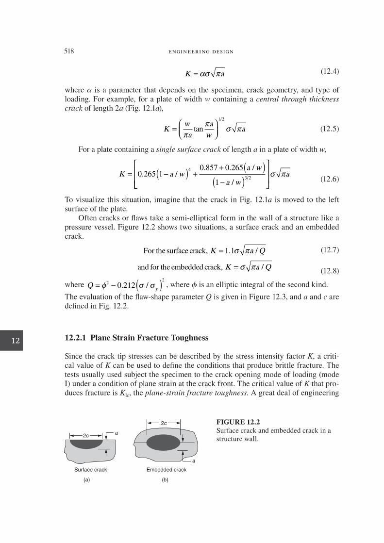
Often cracks or f aws take a semi-elliptical form in the wall of a structure like a pressure vessel. Figure 12.2 shows two situations, a surface crack and an embedded crack.
For thesurface crack, K a Q= 1 1. /σ π (12.7)
and for the embedded crack, K a Q= σ π /
(12.8)
where Qy
= − ( )φ σ σ22
0 212. / , where f is an elliptic integral of the second kind.
The evaluation of the f aw-shape parameter Q is given in Figure 12.3, and a and c are de; ned in Fig. 12.2.
12.2.1 Plane Strain Fracture Toughness
Since the crack tip stresses can be described by the stress intensity factor K , a criti-cal value of K can be used to de; ne the conditions that produce brittle fracture. The tests usually used subject the specimen to the crack opening mode of loading (mode I) under a condition of plane strain at the crack front. The critical value of K that pro-duces fracture is K Ic , the plane-strain fracture toughness . A great deal of engineering
Surface crack Embedded crack
2c
2c
a
a
(a) (b)
FIGURE 12.2
Surface crack and embedded crack in a
structure wall.
die37039_ch12.indd 518 2/25/08 6:58:56 PM

chapter 12: Design with Mater ia ls 519
12
research has gone into standardizing tests for measuring fracture toughness. 6 If a c is the critical crack length at which failure occurs, then
K acIc
= ασ π (12.9)
This is the same as Eq. (12.4), only now a 5 a c and K 5 K Ic , the stress intensity factor required to trigger the fast-moving brittle fracture.
K Ic is a basic material property called plane-strain fracture toughness or often called just fracture toughness . Some typical values are given in Table 12.1.
Note the large difference in K Ic values between the metallic alloys and the poly-mers and the ceramic material silicon nitride. Also, note that the fracture toughness and yield strength vary inversely for the alloy steel and the aluminum alloys. This is a general relationship: as yield strength increases, fracture toughness decreases. It is one of the major constraints in selecting materials for high-performance mechanical applications.
Although K Ic is a basic material property, in the same sense as yield strength, it changes with important variables such as temperature and strain rate. The K Ic of ma-terials with a strong temperature and strain-rate dependence usually decreases with decreased temperature and increased strain rate. The K Ic of a given alloy is strongly dependent on such variables as heat treatment, texture, melting practice, impurity level, and inclusion content.
Equation 12.9 contains the three design variables that must be considered in designing against fracture of a structural component—the fracture toughness, the
FIGURE 12.3
Flaw shape parameter Q for elliptical cracks.
0.5
0.4
a
a
0.3
0.2a/2
c r
atio
0.1
00.7 1.0 1.5
Flaw shape parameter Q
where Q 2 .212
2c 2c
2 A complex flaw
shape parameter
/0 0
/0 0.4
/0 0.6
/0 0.8
/0 1.0
0
2.0 2.5
2
6 . J. D . Landes , “Fracture Toughness Testing,” ASM Handbook, Vol. 8, Mechanical Testing and Evalua-
tion, ASM International , 2000 , pp. 576–85 ; The basic procedure for K Ic testing is ASTM Standard E 399,
“Standard Test Method for Plane Strain Fracture Toughness of Metallic Materials.”
die37039_ch12.indd 519 2/25/08 6:58:57 PM

520 engineering design
12
FIGURE 12.3
Relation between fracture toughness and
allowable stress and crack size.
Crack length a
Allo
wa
ble
str
ess,
=KIc
High KIc
Low KIc
a!
imposed stress, and the crack or f aw size. Figure 12.3 shows the relationship between them. If K Ic is known because the material has been selected, then it is possible to compute the maximum allowable stress to prevent brittle fracture for a given f aw size. Generally the f aw size is determined by actual measurement or by the small-est detectable f aw for the nondestructive inspection method that is available for use. 7 As Fig. 12.3 shows, the allowable stress in the presence of a crack of a given size is directly proportional to K Ic , and the allowable crack size for a given stress is propor-tional to the square of the fracture toughness. Therefore, increasing K Ic has a much larger inf uence on allowable crack size than on allowable stress.
To obtain a proper value of K Ic it must be measured under plane-strain conditions to obtain a maximum constraint or material brittleness. Figure 12.4 shows how the
7. Crack detection sensitivity can vary from 0.5 mm for magnetic particle methods to 0.1 mm for eddy
current, acoustic emission, and liquid penetrant methods. ASM Handbook, Vol. 17, p. 211.
TABLE 12 .1
Some Typical Values of Plane-Strain Fracture
Toughness at Room Temperature
K Ic Yield Strength
MPa m ksi in. MPa ksi
Plain carbon steel AISI 1040 54.0 49.0 260 37.7
Alloy steel AISI 4340
Tempered @ 500°F 50.0 45.5 1500 217
Tempered @ 800°F 87.4 80.0 1420 206
Aluminum alloy 2024-T3 44.0 40.0 345 50
Aluminum alloy 7075-T651 24.0 22.0 495 71
Nylon 6/6 3.0 2.7 50 7.3
Polycarbonate (PC) 2.2 2.0 62 9.0
Polyvinyl chloride (PVC) 3.0 2.2 42 6.0
Silicon nitride—hot pressed 5.0 4.5 800 116
die37039_ch12.indd 520 2/25/08 6:58:57 PM
chapter 12: Design with Mater ia ls 521
12
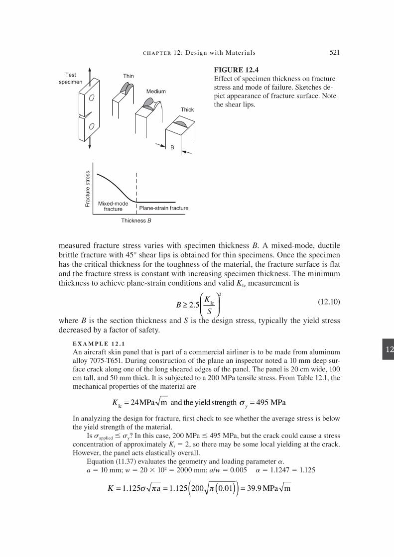
measured fracture stress varies with specimen thickness B . A mixed-mode, ductile brittle fracture with 45° shear lips is obtained for thin specimens. Once the specimen has the critical thickness for the toughness of the material, the fracture surface is f at and the fracture stress is constant with increasing specimen thickness. The minimum thickness to achieve plane-strain conditions and valid K Ic measurement is
BK
S≥
2 5
2
. Ic (12.10)
where B is the section thickness and S is the design stress, typically the yield stress decreased by a factor of safety.
EXAMPLE 1 2 . 1
An aircraft skin panel that is part of a commercial airliner is to be made from aluminum
alloy 7075-T651. During construction of the plane an inspector noted a 10 mm deep sur-
face crack along one of the long sheared edges of the panel. The panel is 20 cm wide, 100
cm tall, and 50 mm thick. It is subjected to a 200 MPa tensile stress. From Table 12.1, the
mechanical properties of the material are
KyIc
MPa m and the yield strength MPa= =24 495σ
In analyzing the design for fracture, ; rst check to see whether the average stress is below
the yield strength of the material.
Is s applied # s y ? In this case, 200 MPa # 495 MPa, but the crack could cause a stress
concentration of approximately K t 5 2, so there may be some local yielding at the crack.
However, the panel acts elastically overall.
Equation (11.37) evaluates the geometry and loading parameter a.
a 5 10 mm; w 5 20 3 10 2 5 2000 mm; a / w 5 0.005 a 5 1.1247 5 1.125
K a= = ( )( ) =1 125 1 125 200 0 01 39 9. . . .σ π π MPa m
FIGURE 12.4
Effect of specimen thickness on fracture
stress and mode of failure. Sketches de-
pict appearance of fracture surface. Note
the shear lips.
Medium
Thick
B
ThinTest
specimen
Thickness B
Mixed-modefracture Plane-strain fracture
Fra
ctu
re s
tre
ss
die37039_ch12.indd 521 2/25/08 6:58:57 PM

522 engineering design
12
Since K $ K Ic , that is, 39.8 $ 24, the panel is expected to fail by a rapid brittle fracture, especially since at 250°F at high altitude the value of K Ic is likely to be much lower than the room temperature value used here.
Solution
Switch to the lower-strength but tougher aluminum alloy 2024 with KIc
MPa m= 44 . For 2024 alloy the yield strength is 345 MPa. This is above the 200 MPa general applied stress, so gross section yielding will not occur. The greater ductility of this alloy will al-low more local plastic deformation at the crack and blunt the crack so the stress concen-tration will not be severe.
As a P nal check we use Eq. (12.10) to see if the plane-strain condition holds for the panel.
BK
y
≥
=
= =2 5 2 5
44
3450 041
2 2
. . .Ic mσ
441mm
This says that the thickness of the panel must be greater than 41 mm to maintain the maximum constraint of the plane-strain condition. A panel with a thickness of 50 mm exceeds this condition.
Another way to look at the problem is to determine the critical crack size at which the crack would propagate to fracture at an average stress of 200 MPa. From Eq. (12.9), and using a value of a 5 1.125, the critical crack length a c is 3.6 mm for the 7075 alumi-num alloy and 12.2 mm for the 2024 alloy . This means that a 7075 alloy sheet with a 10 mm long surface crack would fail in brittle fracture when the 200 MPa stress was applied because its critical crack size is less than 10 mm. However, a 10 mm crack will not cause fracture in the tougher 2024 alloy with a critical crack size of 12.2 mm.
12.2.2 Limitations on Fracture Mechanics
The fracture mechanics concept is strictly correct only for linear elastic materials, that is, under conditions in which no yielding occurs. However, reference to Eqs. (12.2) shows that as r approaches zero, the stress at the crack tip approaches inP nity. Thus, in all but the most brittle material, local yielding occurs at the crack tip and the elastic solution should be modiP ed to account for crack tip plasticity. However, if the plastic zone size r y at the crack tip is small relative to the local geometry, for example, if r y / t or r y / a # 0.1, crack tip plasticity has little effect on the stress intensity factor. That lim-its the strict use of fracture mechanics to high-strength materials. Moreover, the width restriction to obtaining valid measurements of K Ic , as described by Eq. (12.10), makes the use of linear elastic fracture mechanics (LEFM) impractical for low-strength ma-terials. The criterion for LEFM behavior is given by 8
a w a hK
y
, ,−( ) = ≥
42
π σ (12.11)
8. N. E . Dowling , Mechanical Behavior of Materials, 2d ed., Prentice Hall, Upper Saddle River, NJ , 1999 , p. 333.
die37039_ch12.indd 522 2/25/08 6:58:58 PM

chapter 12: Design with Mater ia ls 523
12
where a is the crack length, w is the specimen width, so ( w 2 a ) is the uncracked width and h is the distance from the top of the specimen to the crack. Each of these parameters must satisfy Eq. (12.11). Otherwise the situation too closely approaches gross yielding with the plastic zone extending to one of the boundaries of the speci-men. A value of K determined beyond the applicability of LEFM underestimates the severity of the crack.
Considerable activity has gone into developing tests for measuring fracture tough-ness in materials that have too much ductility to permit the use of LEFM testing methods. 9 The best approach uses the J -integral, which is obtained by measurements of the load versus the displacement of the crack. 10 These tests result in a valid measure of fracture toughness J Ic which serves in the same way as K Ic does for linear elastic materials.
12.3 DESIGN FOR FATIGUE FAILURE
Materials subjected to repetitive or l uctuating stress cycles will fail at a stress much lower than that required to cause fracture on a single application of load. Failures oc-curring under conditions of l uctuating stresses or strains are called fatigue failures . 11 Fatigue accounts for the majority of mechanical failures in machinery.
A fatigue failure is a localized failure that starts in a limited region and propa-gates with increasing cycles of stress or strain until the crack is so large that the part cannot withstand the applied load, and it fractures. Plastic deformation processes are involved in fatigue, but they are highly localized. 12 Therefore, fatigue failure occurs without the warning of gross plastic deformation. Failure usually initiates at regions of local high stress or strain caused by abrupt changes in geometry (stress concentra-tion), temperature differentials, residual stresses, or material imperfections. Much ba-sic information has been obtained about the mechanism of fatigue failure, but at pres-ent the chief opportunities for preventing fatigue lie at the engineering design level. Fatigue prevention is achieved by proper choice of material, control of residual stress, and minimization of stress concentrations through careful design.
Basic fatigue data are presented in the S-N curve, a plot of stress, 13 S, versus the number of cycles to failure, N . Figure 12.5 shows the two typical types of behavior. The curve for an aluminum alloy is characteristic of all materials except ferrous met-als (steels). The S-N curve is chiel y concerned with fatigue failure at high numbers of cycles ( N . 10 5 cycles). Under these conditions the gross stress is elastic, although
9. A . Saxena , Nonlinear Fracture Mechanics for Engineers, CRC Press, Boca Raton, FL , 1998 . 10 . ASTM Standard E 1820. 11. G. E . Dieter , Mechanical Metallurgy, 3d ed., Chap. 12, McGraw-Hill, New York , 1986 ; S . Suresh , Fatigue of Materials, 2d ed., Cambridge University Press, Cambridge , 1998 ; N. E . Dowling , Mechanical
Behavior of Materials, 2d ed., Chaps, 9, 10, 11, Prentice Hall, Englewood Cliffs, NJ , 1999 ; ASM Hand-
book, Vol. 19, Fatigue and Fracture, ASM International, Materials Park, OH , 1996 .
13. It is conventional to denote nominal stresses in fatigue by S rather than s.
12 . ASM Handbook, Vol. 19, Fatigue and Fracture, pp. 63–109 , ASM International, Materials Park, OH , 1996 .
die37039_ch12.indd 523 2/25/08 6:58:58 PM

524 engineering design
12
fatigue failure results from highly localized plastic deformation. Figure 12.5 shows the number of cycles of stress that a material can withstand before failure increases with decreasing stress. For most materials, the S-N curve slopes continuously down-ward toward increasing cycles of stress to failure with decreasing stress. At any stress level there is some large number of cycles that ultimately causes failure. This is called the fatigue strength . For steels in the absence of a corrosive environment, however, the S-N curve becomes horizontal at a certain limiting stress. Below that stress, called the fatigue limit or endurance limit , the steel can withstand an inP nite number of cycles.
12.3.1 Fatigue Design Criteria
There are several distinct strategies concerning design for fatigue that must be under-stood to put this vast subject into proper perspective.
In! nite-life design: This design criterion is based on keeping the stresses below some fraction of the fatigue limit of the steel. This is the oldest fatigue design phi-losophy. It has largely been supplanted by the other strategies discussed below. However, for situations in which steel parts are subjected to very large cycles of uniform stress it is a valid design criterion.
Safe-life design : Safe-life design is based on the assumption that the part is initially l aw-free and has a P nite life in which to develop a critical crack. In this approach to design one must consider that fatigue life at a constant stress is subject to large amounts of statistical scatter. For example, the Air Force historically designed air-craft to a safe life that was one-fourth of the life demonstrated in full-scale fatigue tests of production aircraft. The factor of 4 was used to account for environmen-tal effects, material property variations, and variations in as-manufactured qual-ity. Bearings are another good example of parts that are designed to a safe-life
●
●
FIGURE 12.5
Typical fatigue curves for ferrous and nonferrous metals.
Mild steel
Fatigue limit
Aluminum alloy
105 106
Number of cycles to failure, N
107 108 1090
10
20
30
Ca
lcu
late
d b
en
din
g s
tre
ss,
10
00
psi
40
50
60
die37039_ch12.indd 524 2/25/08 6:58:59 PM

chapter 12: Design with Mater ia ls 525
12
criterion. For example, the bearing may be rated by specifying the load at which 90 percent of all bearings are expected to withstand a given lifetime. Safe-life design also is common in pressure vessel and jet engine design.
Fail-safe design : In fail-safe design the view is that fatigue cracks are likely to oc-cur. Therefore, the structure is designed so that cracks will not lead to failure before they can be detected and repaired. This design philosophy developed in the aircraft industry, where the weight penalty of using large safety factors could not be toler-ated but neither could danger to life from very small safety factors be allowed. Fail-safe designs employ multiple-load paths and crack stoppers built into the structure along with rigid regulations and criteria for inspection and detection of cracks.
Damage-tolerant design : This design philosophy is an extension of the fail-safe approach. In damage-tolerant design, the assumption is that fatigue cracks will ex-ist in an engineering structure. The techniques of fracture mechanics are used to determine whether the cracks will grow large enough to cause failure before they are sure to be detected during a periodic inspection. The emphasis in this design approach is on using materials with high fracture toughness and slow crack growth. The success of the design approach depends upon having a reliable nondestructive evaluation (NDE) program and in being able to identify the damage-critical areas in the design.
Much progress has been made in designing for fatigue, especially through the merger of fracture mechanics and fatigue. Nevertheless, the interaction of many vari-ables that is typical of real fatigue situations makes it inadvisable to depend on a de-sign based solely on analysis. Full-scale prototype testing, often called simulated ser-
vice testing, 14 should be part of all critical designs for fatigue . The failure areas not recognized in design will be detected by these tests. Simulating the actual service loads requires great skill and experience. Often it is necessary to accelerate the test, but doing so may produce misleading results. For example, when time is compressed in that way, the full inl uence of corrosion or fretting is not measured, or the overload stress may appreciably alter the residual stresses. It is common practice to eliminate many small load cycles from the load spectrum, but they may have an important inl u-ence on fatigue crack propagation.
12.3.2 Fatigue Parameters
Typical cycles of stress that produce fatigue failure are shown in Fig. 12.6. Figure 12.6 a illustrates a completely reversed cycle of stress of sinusoidal form. This is the type of fatigue cycle for which most fatigue property data is obtained in laboratory testing. 15 It is found in service by a rotating shaft operating at constant speed without overloads. For this type of stress cycle the maximum and minimum stresses are equal. In keeping with convention, the minimum stress is the lowest algebraic stress in the
●
●
14 . R. M . Wetzel (ed.)., Fatigue Under Complex Loading, Society of Automotive Engineers, Warren-dale, PA , 1977 . 15 . Common types of fatigue testing machines are described in many references in this section and in ASM Handbook, Vol. 8, pp. 666–716 , ASM International , 2000 .
die37039_ch12.indd 525 2/25/08 6:58:59 PM

526 engineering design
12
cycle. Tensile stress is considered positive, and compressive stress is negative. Figure 12.6 b illustrates a repeated stress cycle in which the maximum stress smax and mini-mum stress smin are not equal. In this illustration they are both tension, but a repeated stress cycle could just as well contain maximum and minimum stresses of opposite signs or both in compression. Figure 12.6 c illustrates a complicated stress cycle that might be encountered in a part such as an aircraft wing, which is subjected to periodic unpredictable overloads due to wind gusts.
A l uctuating stress cycle can be considered to be made up of two components, a mean , or steady, stress, s m , and an alternating , or variable, stress, s a . We must also consider the range of stress, s r . As can be seen from Fig. 12.6 b , the range of stress is the algebraic difference between the maximum and minimum stress in a cycle.
σ σ σr
= −max min (12.12)
The alternating stress, then, is one-half of the range of stress.
σσ σ σ
a
r= =−
2 2max min (12.13)
The mean stress is the algebraic mean of the maximum and minimum stress in the cycle.
σσ σ
m=
+max min
2 (12.14)
FIGURE 12.6
Typical fatigue stress cycles: (a) reversed stress; (b) repeated stress; (c) irregular or random stress cycle.
Cycles
2 C
om
pre
ssio
nStr
ess
Str
ess
Te
nsio
n 1
0
1
2
1
2
(a)
!a
!r
!max
!f
!m
!z
!min
Cycles
(c)
Cycles
(b)
die37039_ch12.indd 526 2/25/08 6:58:59 PM

chapter 12: Design with Mater ia ls 527
12
A convenient way to denote the fatigue cycle is with the stress ratio , R .
R = σ σmin max
/ (12.15)
For a completely reversed stress cycle, s max 5 2s min , R 5 21, and s m 5 0. For a fully tensile repeated stress cycle with s min 5 0, R 5 0. The inl uence of mean stress on the S-N diagram can be expressed by the Goodman equation.
σ σσσa e
m
uts
= −
1 (12.16)
where s e is the endurance limit in a fatigue test with a completely reversed stress cycle, and s uts is the ultimate tensile strength.
Fatigue is a complex material failure process. The fatigue performance of a com-ponent depends on the following important engineering factors:
Stress Cycle
Repeated or random applied stress Mean stress. Most fatigue test data has been obtained under completely repeated stress with a mean stress of zero.
Combined stress state Stress concentration. Most fatigue cracks start at points of elevated stress. This is expressed by a stress concentration factor (for the geometry) and a notch sensitivity
factor for the material’s sensitivity for stress concentrations. Statistical variation in fatigue life and fatigue limit. There is more scatter in fatigue life than in any other mechanical property of materials.
Cumulative fatigue damage. The conventional fatigue test subjects a specimen to a P xed amplitude of stress until the specimen fails. However, in practice there are many situations where the cyclic stress does not remain constant, but instead there are periods when the stress is either above or below some average design level. Tak-ing into consideration irregular stress versus cycle issues is an important area of fatigue design for which additional concepts are needed.
Component or Specimen-Related Factors
Size effect. The larger the section size of the part, the lower its fatigue properties. This is related to the higher probability of P nding a critical crack-initiating l aw in a larger volume of material.
Surface P nish. Most fatigue cracks start at the surface of a component. The smoother the surface roughness, the higher is the fatigue property.
Residual stress. Residual stresses are locked-in stresses that are present in a part when it is not subjected to loads, and which add to the applied stresses when un-der load. The formation of a compressive residual distribution on the surface of a part is the most effective method of increasing fatigue performance. The best way of doing this is shot blasting or rolling of the surface to cause localized plastic deformation.
Surface treatment. As noted above, surface treatments that increase the compres-sive residual stresses at the surface are beneP cial. Increasing the surface hardness
●
●
●
●
●
●
●
●
●
●
die37039_ch12.indd 527 2/25/08 6:58:59 PM

528 engineering design
12
by carburizing or nitriding often improves the fatigue performance of steel parts. However, losing carbon from the surface of steel by poor heat treatment practice is detrimental to fatigue properties.
Environmental Effects
Corrosion fatigue. The simultaneous action of cyclic stress and chemical attack is known as corrosion fatigue . Corrosive attack without superimposed stress often produces pitting of metal surfaces. The pits act as notches and produce a reduc-tion in fatigue strength. However, when corrosive attack occurs simultaneously with fatigue loading, a very pronounced reduction in fatigue properties results that is greater than that produced by prior corrosion of the surface. When corrosion and fatigue occur simultaneously, the chemical attack greatly accelerates the rate at which fatigue cracks propagate. Steels that have a fatigue limit when tested in air at room temperature show no indication of a fatigue limit in corrosion fatigue.
Fretting fatigue. Fretting is the surface damage that results when two surfaces in contact experience slight periodic relative motion. The phenomenon is more related to wear than to corrosion fatigue. However, it differs from wear by the facts that the relative velocity of the two surfaces is much lower than is usually encountered in wear and that since the two surfaces are never brought out of contact, there is no chance for the corrosion products to be removed. Fretting is frequently found on the surface of a shaft with a press-P tted hub or bearing. Surface pitting and deteriora-tion occur, usually accompanied by an oxide debris (reddish for steel and black for aluminum). Fatigue cracks often start in the damaged area.
Space precludes further discussion of these factors. The reader is referred to the basic references at the beginning of this section for details on how the factors control fatigue.
12.3.3 Information Sources on Design for Fatigue
There is a considerable literature on design methods to prevent fatigue failure. Most machine design texts devote a chapter to the subject. In addition, the following spe-cialized texts add a great deal of detail.
Fatigue design for inP nite life is considered in:
R. C. Juvinall, Engineering Consideration of Stress, Strain, and Strength, McGraw-Hill, New York, 1967. Chapters 11 to 16 cover fatigue design in con-siderable detail.
L. Sors, Fatigue Design of Machine Components, Pergamon Press, New York, 1971. Translated from the German, this presents a good summary of European fatigue design practice.
C. Ruiz and F. Koenigsberger, Design for Strength and Production, Gordon & Breach Science Publishers, New York, 1970. Pages 106 to 120 give a concise discussion of fatigue design procedures.
●
●
die37039_ch12.indd 528 2/25/08 6:59:00 PM

chapter 12: Design with Mater ia ls 529
12
Detailed information on stress concentration factors and the design of machine details to minimize stress can be found in:
W. D. Pilkey, Peterson’s Stress Concentration Factors, 2d ed., John Wiley & Sons, New York, 1997.
R. B. Heywood, Designing Against Fatigue of Metals, Reinhold, New York, 1967.
C. C. Osgood, Fatigue Design, 2d ed., Pergamon Press, New York, 1982.
The most complete books on fatigue design, including the more modern work on safe-life design and damage-tolerant design, are:
H. O. Fuchs and R. I. Stephens, Metal Fatigue in Engineering, John Wiley & Sons, New York, 1980.
Fatigue Design Handbook, 3d ed., Society of Automotive Engineers, Warrendale, PA, 1997.
E. Zahavi, Fatigue Design, CRC Press, Boca Raton, FL, 1996.
A useful web site for fatigue data and helpful calculators is www.fatiguecalculator.com
Several design examples are presented in the next few sections.
12.3.4 InC nite Life Design 16
This section considers the design for fatigue of components that are assumed to be able to withstand an inP nite number of stress cycles if the maximum stress is kept below the fatigue (endurance) limit. For materials that do not have a deP ned fatigue limit, such as the aluminum alloy shown in Fig. 12.5, the design is based on fatigue
strength , deP ned as the stress amplitude that the material can support for at least 10 8 fatigue cycles.
E X A M P L E 1 2 . 2
A steel shaft heat-treated to a Brinell hardness of 200 has a major diameter of 1.5 in. and a small diameter of 1.0 in. There is a 0.10-in. radius at the shoulder between the diameters. The shaft is subjected to completely reversed cycles of stress of pure bending. The fatigue limit determined on polished specimens of 0.2-in. diameter is 42,000 psi. The shaft is produced by machining from bar stock. What is the best estimate of the fatigue limit of the shaft?
Since an experimental value for fatigue limit is known, we start with it, recogniz-ing that tests on small, unnotched polished specimens represent an unrealistically high value of the fatigue limit of the actual part. 17 The procedure, then, is to factor down the idealized value. We start with the stress concentration (notch) produced at the shoulder
16 . Based on design procedures described by R. C . Juvinall , Engineering Consideration of Stress,
Strain, and Strength, McGraw-Hill, New York , 1967 . 17. If fatigue property data are not given, they must be determined from the published literature or estimated from other mechanical properties of the material; see H. O . Fuchs and R. I . Stephens , Metal
Fatigue in Engineering, pp. 156–160 , John Wiley & Sons, New York , 1980 ; ASM Handbook, Vol. 19, 1996 , pp. 589–955 .
die37039_ch12.indd 529 2/25/08 6:59:00 PM

530 engineering design
12
18. R. C . Juvinall , op. cit., p. 234 . 19. G . Castleberry , Machine Design, pp. 108–110 , Feb. 23, 1978 .
between two diameters of the shaft. A shaft with a P llet in bending is a standard situation covered in all machine design books. If D 5 1.5, d 5 1.0, and r 5 0.10, the important ratios are D / d 5 1.5 and r / d 5 0.1 . Then, from standard curves, the theoretical stress
concentration factor is K t 5 1.68. However, K t is determined for a brittle elastic solid, and most ductile materials exhibit a lesser value of stress concentration when subjected to fa-tigue. The extent to which the plasticity of the material reduces K t is given by the fatigue
notch sensitivity q .
qK
Kf
t
=−−
1
1 (12.17)
where K t 5 theoretical stress concentration factor
Kf
= =fatigue notch factorfatigue limit unnotched
ffatigue limit notched
From design charts we P nd that a steel with a Brinell hardness of 200 has a q of 0.8. From Eq. (12.17), K f is 1.54. This information will be used later in the design.
Returning to the fatigue limit for a small polished specimen, S e 5 42,000 psi, we need to reduce this value because of size effect, surface P nish, and type of loading and for statistical scatter
S S C C C C
C
C
S F L Z
S
F
e e′ =
=where factor for size effect
===
factor for surface finish
factor for typeCL
oof loading
factor for statistical scatterCZ
=
(12.18)
Increasing the specimen size increases the probability of surface defects, and hence the fatigue limit decreases with increasing size. Typical values of C S are given inTable 12.2. In this example we use C S 5 0.9.
Curves for the reduction in fatigue limit due to various surface P nishes are available in standard sources. 18 For a standard machined P nish in a steel of BHN 200, C F 5 0.8.
Laboratory fatigue data (as opposed to simulated service fatigue tests) commonly are determined in a reversed bending loading mode. Other types of loading, such as axial and torsional, generate different stress gradients and stress distributions and do not produce the same fatigue limit for the same material. Thus, fatigue data generated in reversed bending must be corrected by a load factor C L , if the data are to be used in a different loading mode. Table 12.3 gives typical values. Since the bending fatigue data are used for an application involving bending, C L 5 1.0.
Fatigue tests show considerable scatter in results. Fatigue limit values are normally distributed with a standard deviation that can be up to 8 percent of the mean value. If the test or literature value is taken as the mean value of fatigue limit (which in itself is a big assumption), then this value is reduced by a statistical factor 19 according to the reliability level that is desired (Table 12.4).
die37039_ch12.indd 530 2/25/08 6:59:00 PM
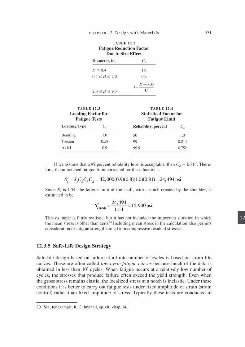
chapter 12: Design with Mater ia ls 531
12
If we assume that a 99 percent reliability level is acceptable, then C Z 5 0.814. There-fore, the unnotched fatigue limit corrected for these factors is
′ = = =S S C C Ce e S F Z
42 000 0 9 0 8 1 0 0 81 24, ( . )( . )( . )( . ) ,,494 psi
Since K f is 1.54, the fatigue limit of the shaft, with a notch created by the shoulder, is estimated to be
′ = =Se,
,
.,
notchpsi
24 494
1 5415 900
This example is fairly realistic, but it has not included the important situation in which the mean stress is other than zero. 20 Including mean stress in the calculation also permits consideration of fatigue strengthening from compressive residual stresses.
12.3.5 Safe-Life Design Strategy
Safe-life design based on failure at a P nite number of cycles is based on strain-life curves. These are often called low-cycle fatigue curves because much of the data is obtained in less than 10 5 cycles. When fatigue occurs at a relatively low number of cycles, the stresses that produce failure often exceed the yield strength. Even when the gross stress remains elastic, the localized stress at a notch is inelastic. Under these conditions it is better to carry out fatigue tests under P xed amplitude of strain (strain control) rather than P xed amplitude of stress. Typically these tests are conducted in
TABLE 12 . 3
Loading Factor for
Fatigue Tests
Loading Type C L
Bending 1.0
Torsion 0.58
Axial 0.9
TABLE 12 .4
Statistical Factor for
Fatigue Limit
Reliability, percent C Z
50 1.0
99 0.814
99.9 0.752
TABLE 12 .2
Fatigue Reduction Factor
Due to Size Effect
Diameter, in. C S
D # 0.4 1.0
0.4 # D # 2.0 0.9
2.0 # D # 9.0 1
0 03
15− −D .
20. See, for example, R. C . Juvinall , op. cit., chap. 14.
die37039_ch12.indd 531 2/25/08 6:59:01 PM

532 engineering design
12
push-pull tension. Figure 12.7 shows the stress-strain loop that is produced by strain control cycling. The strain amplitude is given by
ε ε ε εa
e p= = +∆ ∆ ∆2 2 2
(12.19)
where the total strain ∆e is the sum of the elastic and plastic strains and the strain am-plitude is one-half of the total strain.
A plot of the stress at the tip of the stress-strain loop (point B ) for various strain amplitudes yields a cyclic true stress-strain curve. When plotted on log-log coordi-nates this yields a straight line for strain amplitudes beyond the dynamic yield stress (point C ). The stress amplitude is given by
∆ ∆σ ε2 2
= ′
′
kp
n
(12.20)
where k 9 is the cyclic strength coef! cient (the intercept of the line on the stress axis) and n 9 , the slope of the line, is the cyclic strain hardening exponent . Substituting into Eq. (12.19) from Eq. (12.20) gives
∆ ∆ ∆ε σ σ2 2 2
1
= +′
′
E k
n/
(12.21)
Equation (12.21) allows the calculation of the cyclic stress-strain curve. Values of the material properties E , k9 and n 9 are available in the literature. 21
The strain-life curve plots the total strain amplitude versus the number of strain
reversals to failure, Fig 12.8. Both the elastic and plastic curves are approximated as straight lines. At small strains or long lives, the elastic strain predominates, and at large strains or short lives the plastic strain is predominant. The plastic curve has a
21. ASM Handbook, Vol. 19, pp. 963–79.
FIGURE 12.7
Typical cyclic stress-strain loop.
2
!
re"ee"
e
e
"
O
A
C
B
2
!"
2
!"2
e"
die37039_ch12.indd 532 2/25/08 6:59:01 PM

chapter 12: Design with Mater ia ls 533
12
negative slope of c and an intercept at 2 N 5 1. The elastic curve has a negative slope of b and an intercept of ′σ
fE/ . The equation for the elastic line is
log log logˆ∆ ∆ε σ
e f
fE
b N2
2
=
′
+ ( )or
εε σe f
f
b
EN
22=
′ ( )
Similarly, the plastic line is given by ∆ε εp
f f
c
N2
2= ′ ( ) . But, from Eq. (12.19),
ε ε σε
a
f
f
b
f f
c
EN N= =
′ ( ) + ′ ( )∆2
2 2 (12.22)
The exponent b ranges from about 20.06 to 20.14 for different materials, and a typi-cal value is 20.1. The exponent c ranges from about 20.5 to 20.7, and 20.6 is a rep-resentative value. The term e9f , called the fatigue ductility coef! cient , is approximately equal to the true fracture strain measured in the tension test. Likewise, the fatigue
strength coef! cient s9f is approximated by the true fracture stress. An important use of the low-cycle fatigue approach is to predict the life to crack
initiation at notches in machine parts where the nominal stresses are elastic but the local stresses and strain at the notch root are plastic. When there is plastic deforma-tion, both a strain concentration Ke and a stress concentration K s must be considered. Neuber’s rule relates these by22
K K Kf
= ( )σ ε
1 2/ (12.23)
where K f is the fatigue notch factor.
FIGURE 12.8
Typical strain-life curve for mild steel.
efe9
f!9
E
c
b
100 101 102 103
Reversals to failure, 2Nf
log scale
Str
ain
am
plit
ud
e,
"
/2
log
sca
le
Plastic
Total = elastic and plastic
Elastic
2Nt
104 105 106 107
22 . The number of strain reversals equals twice the number of strain cycles.
die37039_ch12.indd 533 2/25/08 6:59:02 PM

534 engineering design
12
The situation is described in Fig. 12.9, where ∆S and ∆e are the elastic stress and strain increments at a location remote from the notch and ∆s and ∆e are the local stress and strain at the root of the notch.
KS
Keσ ε
σ ε= =∆∆
∆∆
and
KS e
E
S Ef=
=
∆ ∆∆ ∆
∆ ∆∆ ∆
σ ε σ εε
1 2 1 2/ /
and K S eE Ef
∆ ∆ ∆ ∆( ) = ( )1 2 1 2/ /
σ ε (12.24)
For nominally elastic loading, ∆ S 5 ∆ eE and
K S Ef∆ ∆ ∆= ( )σ ε
1 2/ (12.25)
Thus, Eq. (12.25) allows stresses remotely measured from the notch to be used to predict stress and strain at the notch. Rearranging Eq. (12.25) gives
∆ ∆∆
σ ε =( )
=K S
E
f
2
constant (12.26)
which is the equation of a rectangular hyperbola (Fig. 12.9 c ). If a nominal stress S 1 is applied to the notched specimen (Fig. 12.9b), then the right side of Eq. (12.26) is known provided K f is known. The cyclic stress-strain curve also is plotted in Fig. 12.9 c (solid curve), and its intersection with Eq. (12.26) gives the local stress and strain at the notch root.
The use of Neuber’s analysis to P nd the stress and strain at a notch in conjunc-tion with the strain-life curve (Fig. 12.8) is a widely accepted approach to predicting the number of fatigue cycles to the initiation of a crack. The basic assumption is that
FIGURE 12.9
Stress analysis at a notch using Neuber’s analysis.
P
P
(a) (b)
S
S
S
"
"
SK( )
E=
"
S"e"
e"
(c)
2
1
!
"! "e
"!"e
"ee
!
1f
die37039_ch12.indd 534 2/25/08 6:59:02 PM
chapter 12: Design with Mater ia ls 535
12
the local fatigue response at the critical region, usually at a l aw or geometric notch, is similar to the fatigue response of a small, smooth laboratory specimen subjected to the same cyclic strains and stresses as the critical region.
To use the prediction model it is necessary to
Compute with FEA the local stresses and strains, including mean stress and stress range.
Count the cycles and corresponding mean and range values of stress and strain. Nonzero mean cycles must be converted to equivalent completely reversed cycles. Have appropriate material properties to compute fatigue damage during each cycle.
Sum the damage to give the prediction of the number of cycles to crack initiation.
E X A M P L E 1 2 . 3 Use of Neuber Analysis and Strain-Life Curve.
A hot-rolled 4340 steel plate has the following mechanical properties: s ult 5 826 MPa;
s y 5 634 MPa; E 5 206 GPa 5 206 3 10 3 MPa; ′ = = − = − ′ =εf
b c n0 53 0 10 0 56 0 17. ; . ; . ; . ;
′ = ′ =kf
1384 1232MPa MPa.; σ The plate is loaded in tension by a completely reversed
axial force of 500,000 N. The plate has a single edge notch with a fatigue stress con-centration factor of K f 5 1.8. At the notch the plate is 20 mm thick and the net width is 101.6 mm.
The nominal stress amplitude is SP
Aa
= =×
= =500 000
20 101 6246 246
,
.N/mm MPa.2 Thus,
the nominal stress range is ∆S Sa
= = =2 2 246 492( ) MPa, from Fig. 12.7. From Eq. (12.26)
∆ ∆σ ε = ××
=( . ).
1 8 492
206 103 8
2
2MPa
From the relationship for the cyclic stress-strain curve, Eq. (12.21),
∆ ∆ ∆∆
∆ ∆∆
ε σ εε
σ εε2 2 206 10 2 13843
1 0
=×
+×
( )
/ .117
3 8
and since has been found above
to be MPa,
∆ ∆σ ε
.
∆∆∆ ∆
εε ε
=×
+
3 8
206 10
12
3 8
2 1384
13
5 88
. .
( )
.
Using iteration to solve for ∆e, the strain range is found to be 4.026 3 10 23 mm/mm.
Now we can use the equation for the strain-life curve, Eq. (12.22), to estimate the number of cycles to initiate a fatigue crack, N i . Substituting the parameters for the strain-life curve,
4 026 10
2
1232
206 102 0 53 2
3
3
0 10..
.× =×
( ) + ( )−
−N N
i i
−−
− − − −× = × +
0 56
3 3 0 102 013 10 5 580 10 0 360
.
.. . .N Ni i
00 56
0 10 0 560 361 64 5
0 366 6
.
. .. .
.
and
N N
N
i i
i
− −= −
= − 55 5 0 561 0 10
. ./ .
Ni
− −( )
●
●
●
●
●
die37039_ch12.indd 535 2/25/08 6:59:02 PM

536 engineering design
12
Solving the preceding equation by iteration, the number of cycles to initiate a crack about 1 mm long is 2.104 3 10 5 cycles.
Using this method in more realistic design situations would require correcting the results for the presence of mean stress, and for treating less regular cycles of fatigue stress. 23 Strain-life analysis has found broad acceptance in the automotive and aero-space industries for component design in the early stages of embodiment design. It allows reasonable prediction of fatigue life in design before components are available for actual fatigue resting, which results in a reduction in the number of design itera-tions and a speedup in the PDP cycle. A number of specialized computer programs are available to assist in the design analysis.
12.3.6 Damage-Tolerant Design Strategy
Damage-tolerant design starts with the premise that the part contains a fatigue crack of known dimensions and geometry and predicts how many cycles of service are available before the crack will propagate to a catastrophic size that will cause failure, N p . Thus, the emphasis is on fatigue crack growth. Figure 12.10 shows the process of crack propagation from an initial crack of length a 0 to a crack of critical l aw size a cr . The crack growth rate da / dN increases with the cycles of repeated load.
An important advance in fatigue design was the realization that the fatigue crack growth rate da / dN can be related to the range of the stress intensity factor; ∆ K 5 K max 2 K min , for the fatigue cycle. Since the stress intensity factor K a= ασ π is unde-P ned in compression, K min is taken as zero if s min is compression in the fatigue cycle.
Figure 12.11 shows a typical plot of rate of crack growth versus ∆ K . The typical curve is sigmoidal in shape with three distinct regions. Region I contains the thresh-old value ∆ K th below which there is no observable crack growth. Below ∆ K th, fatigue cracks behave as nonpropagating cracks. The threshold starts at crack propagation
rates of around l0 28 in./cycle and at very low values of K , for example 8 ksi in. for stress. Region II exhibits essentially a linear relation between log da / dN and log K , which results in
da
dNA K
n
n= ( )
=
∆
where slopeof the curve in region II
AA = coefficient found by extending the line tto ksi in.∆K = 1
(12.27)
Region III is a region of rapid crack growth that is soon followed by fracture. The relation between fatigue crack growth ∆ K and expressed by Eq. (12.27) ties
together fatigue design 24 and linear elastic fracture mechanics (LEFM). The elastic stress intensity factor is applicable to fatigue crack growth even in low-strength, high-
23. Y-L Lee , J . Pan ., R . Hathaway , and M . Barkey , Fatigue Testing and Analysis, Chap. 5, Elsevier, Boston , 2005 .
24. R. P . Wei , Trans. ASME, Ser. H., J. Eng. Materials Tech., vol. 100, pp. 113–20 , 1978 ; A. F . Liu , Structural Life Assessment Methods, ASM International, Materials Park, OH , 1998 .
die37039_ch12.indd 536 2/25/08 6:59:03 PM
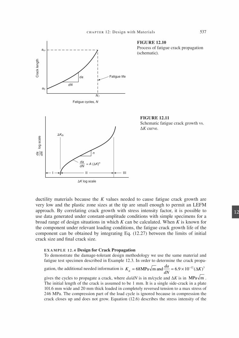
chapter 12: Design with Mater ia ls 537
12
ductility materials because the K values needed to cause fatigue crack growth are very low and the plastic zone sizes at the tip are small enough to permit an LEFM approach. By correlating crack growth with stress intensity factor, it is possible to use data generated under constant-amplitude conditions with simple specimens for a broad range of design situations in which K can be calculated. When K is known for the component under relevant loading conditions, the fatigue crack growth life of the component can be obtained by integrating Eq. (12.27) between the limits of initial crack size and P nal crack size.
E X A M P L E 1 2 . 4 Design for Crack Propagation
To demonstrate the damage-tolerant design methodology we use the same material and fatigue test specimen described in Example 12.3. In order to determine the crack propa-
gation, the additional needed information is Kda
dNK
Ic= = × −68 6 9 10 12 3MPa m and . ( )∆
gives the cycles to propagate a crack, where da / dN is in m/cycle and ∆ K is in MPa m . The initial length of the crack is assumed to be 1 mm. It is a single side-crack in a plate 101.6 mm wide and 20 mm thick loaded in completely reversed tension to a max stress of 246 MPa. The compression part of the load cycle is ignored because in compression the crack closes up and does not grow. Equation (12.6) describes the stress intensity of the
FIGURE 12.10
Process of fatigue crack propagation (schematic).
Fatigue life
Fatigue cycles, N
Cra
ck le
ng
th
acr
a0
da
dN
N f
FIGURE 12.11
Schematic fatigue crack growth vs. ∆K curve.
da
dN
log
sca
le
"K log scale
da
dN
n
= A ("K)n
"Kth
die37039_ch12.indd 537 2/25/08 6:59:03 PM

538 engineering design
12
crack and is evaluated to be K a= 1 15. .σ π From Eq. (12.9) the P nal crack length at fracture, a f , is
a aK
c f= =
=
× 1
1 15
1 68
1 15 246
2
π σ πIc
. .max = =
2
0 018 18. m mm
Now use the equation for the propagation of a crack in region II in a 4340 steel plate. Also,
∆
∆
K K K a
da
dNK
= − =
= × =−
max min .
. ( ) .
1 15
6 9 10 6 912 3
σ π
×× ×
= ×
−
−
10 1 15 246
868 10
12 3 3 2 3 2
1 5
6
( . ) ( ) / /
.
π a
da
addN
a daa
a
a f −
=
= − +
∫ =− +
1 5
0 001
0 0181 5 1
0 1 5 1
.
.
..
. 0..001
0.018 = ×
−−
−
−
868 10
0 018
0 5
0 001
6
0
0 5
N NP
.
.
.. −−−
−
−= ×
=×
= ×
0 56
6
0 5868 10
48 338
868 105 56
.
.
..
N
N
P
P 1104 cycles
The total fatigue life to failure, N f , is the sum of the number of cycles to initiate a crack, N i , and the cycles to grow the crack until complete fracture occurs, N p . For the problem given in Examples 12.3 and 12.4, N f 5 N i 1 N p 5 2.104 3 10 5 1 5.56 3 10 4 5 2.660 3 10 5 cycles. Note that under the given conditions the crack initiation stage is about one order of magnitude larger than the crack propagation stage.
12.3.7 Further Issues in Fatigue Life Prediction
The three preceding examples have illustrated the major approaches for dealing with fatigue failure in design. The presentation has been necessarily brief and basic. Using these design strategies most likely will require further study of topics such as:
Accounting for geometric stress concentrations and stress gradients Making allowance for the presence of compressive residual stresses that are either purposely introduced to improve fatigue performance or harmful tensile residual stresses that are introduced by manufacturing processes
Further consideration of the case when the mean stress is not zero Calculation for situations of two- or three-dimensional states of fatigue stresses Accounting for nonregular stress cycles, and for random cycles of stress.
The many references given in this section will be helpful in gaining this knowledge, while computer design software for fatigue will remove some of the drudgery inherent in these kinds of calculations.
●
●
●
●
●
die37039_ch12.indd 538 2/25/08 6:59:03 PM

chapter 12: Design with Mater ia ls 539
12
12.4 DESIGN FOR CORROSION RESISTANCE
Failure of metal components by corrosion is as common as failure due to mechani-cal causes, such as brittle fracture and fatigue. The National Institute of Standards and Technology estimates that corrosion annually costs the United States $70 billion, of which at least $10 billion could be prevented by better selection of materials and design procedures. Although corrosion failures are minimized by proper materials selection and careful attention to control of metallurgical structure through heat treat-ment and processing, many corrosion-related failures can be minimized by proper understanding of the interrelation of the fundamental causes of corrosion and design details. 25
12.4.1 Basic Forms of Corrosion
Corrosion of metals is driven by the basic thermodynamic force of a metal to return to the oxide or sulP de form, but it is more related to the electrochemistry of the reac-tions of a metal in an electrolytic solution (electrolyte). There are eight basic forms of corrosion. 26
Uniform attack. The most common form of corrosion is uniform attack. It is char-acterized by a chemical or electrochemical reaction that proceeds uniformly over the entire exposed surface area. The metal becomes thinner, leading to eventual failure.
Galvanic corrosion. The potential difference that exists when two dissimilar metals are immersed in a corrosive or conductive solution is responsible for galvanic corrosion. The less-resistant (anodic) metal is corroded relative to the cathodic metal. Table 12.5 gives a brief galvanic series for some commercial alloys immersed in sea-water. In this table, for any two metals or alloys in contact in seawater, the metal that is more anodic (lower in the series) will be corroded. Note that the relative position in a galvanic series depends on the electrolytic environment as well as the metal’s sur-face chemistry (presence of passive surface P lms).
Use pairs of metals that are close together in the galvanic series to minimize galvanic corrosion and avoid situations in which a small anodic area of metal is con-nected to a larger surface area of more noble metal. If two metals far apart in the series must be used in contact, they should be electrically insulated from each other. Do not coat the anodic surface to protect it, because most coatings are susceptible to pinholes. The coated anode surface would corrode rapidly in contact with a large cathodic area. When a galvanic couple is unavoidable, consider utilizing a third metal that is anodic and sacriP cial to both of the other metals.
25. V. P . Pludek , Design and Corrosion Control, John Wiley & Sons, New York , 1977 . 26. M. G . Fontana and N. D . Greene , Corrosion Engineering, 3d ed., McGraw-Hill, New York , 1986 .
die37039_ch12.indd 539 2/25/08 6:59:04 PM

540 engineering design
12
Crevice corrosion. An intense localized corrosion frequently occurs within crev-ices and other shielded areas on metal surfaces exposed to corrosive attack. This type of corrosion usually is associated with small volumes of stagnant liquid trapped in design features such as holes, gasket surfaces, lap joints, and crevices under bolt and rivet heads.
Pitting. Pitting is a form of extremely localized corrosive attack that produces holes in the metal. It is an especially insidious form of corrosion because it causes equipment to fail after exposure to only a small percentage of the designed-for weight loss.
Intergranular corrosion. Localized attack along the grain boundaries with only slight attack of the grain faces is called intergranular corrosion. It is especially com-mon in austenitic stainless steel that has been sensitized by heating to the range 950 to 1450°F. It can occur either during heat treatment for stress relief or during welding. When it occurs during welding it is known as weld decay .
Selective leaching. The removal of one element from a solid-solution alloy by corrosion processes is called selective leaching. The most common example of it is the selective removal of zinc from brass (dezinciP cation), but aluminum, iron, cobalt, and chromium also can be removed. When selective leaching occurs, the alloy is left in a weakened, porous condition.
TABLE 12 .5
A Brief Galvanic Series for Commercial
Metals and Alloys
Noble (cathodic) Platinum
Gold
Titanium
Silver
316 stainless steel
304 stainless steel
410 stainless steel
Nickel
Monel
Cupronickel
Cu-Sn bronze
Copper
Cast iron
Steel
Active (anodic) Aluminum
Zinc
Magnesium
die37039_ch12.indd 540 2/25/08 6:59:04 PM

chapter 12: Design with Mater ia ls 541
12
Erosion-corrosion. Deterioration at an accelerated rate is caused by relative movement between a corrosive l uid and a metal surface; it is called erosion- corrosion. Generally the l uid velocity is high and mechanical wear and abrasion may be involved, especially when the l uid contains suspended solids. Erosion destroys protective sur-face P lms and exacerbates chemical attack. Design plays an important role in erosion control by creating form alterations to reduce l uid velocity, eliminating situations in which direct impingement occurs, and minimizing abrupt changes in the direction of l ow. Some erosion situations are so aggressive that neither selection of a suitable ma-terial nor design can ameliorate the problem. Here the role of design is to provide for easy detection of damage and for quick replacement of damaged components.
A special kind of erosion-corrosion is cavitation , which arises from the formation and collapse of vapor bubbles near the metal surface. Rapid bubble collapse can pro-duce shock waves that cause local deformation of the metal surface.
Another special form of erosion-corrosion is fretting corrosion . It occurs between two surfaces under load that are subjected to cycles of relative motion. Fretting pro-duces breakdown of the surface into an oxide debris and results in surface pits and cracks that usually lead to fatigue cracks.
Stress-corrosion cracking. Cracking caused by the simultaneous action of a tensile stress and contact with a speci! c corrosive medium is called stress-corrosion cracking (SCC). The stress may be a result of applied loads or “locked-in” residual stress. Only speciP c combinations of alloys and chemical environments lead to stress-corrosion cracking. However, many occur commonly, such as aluminum alloys and seawater, copper alloys and ammonia, mild steel and caustic soda, and austenitic steel and salt water. 27 Over 80 combinations of alloys and corrosive environments are known to cause stress-corrosion cracking. Design against stress-corrosion cracking involves selecting an alloy that is not susceptible to cracking in the service environ-ment; but if that is not possible, then the stress level should be kept low. The concepts of fracture mechanics have been applied to SCC.
12.4.2 Corrosion Prevention
Material Selection. Selecting a material with a low rate of corrosion in the en-vironment of concern is the obvious P rst step to preventing corrosion. In general, the more noble the metal the slower it will corrode (see Table 12.5). The brief discussion of the corrosion mechanisms in Sec. 12.4.1 provides some insight, but there is a vast literature on corrosion, much of it compiled in handbook form 28 and in databases. 29
27. G. H . Koch , ASM Handbook, Vol. 19, pp. 483–506 , ASM International, Materials Park, OH , 1996 . 28. ASM Handbooks, Vol. 13: Vol. 13A, Corrosion Fundamentals, Testing, and Protection; Vol. 13B, Corrosion: Materials ( provides extensive data on corrosion performance of metals and nonmetals); Vol. 13C, Corrosion: Environments and Industries (focuses on corrosion in speciP c environments and in speciP c industries). The Cambridge Engineering Selector software is a good place to do a P rst screen for corrosion properties. 29. For an excellent compilation of sources, see ASM Handbook, Vol. 13A, pp. 999–1001 .
die37039_ch12.indd 541 2/25/08 6:59:04 PM

542 engineering design
12
Metals are the most susceptible to corrosion, while plastics in general have much cor-rosion resistance. Some polymers absorb moisture, which causes swelling and degra-dation of mechanical properties.
While some aspects of material selection for corrosion are straightforward—for example, avoiding materials that are attacked in the corrosive environment of interest or are subject to SCC in the environment—other aspects of corrosion can be quite subtle. Microscopic galvanic cells can be created in metallic alloys due to such things as microsegregation of alloying elements (especially at grain boundaries), local cold-worked regions, or differences in galvanic potential between phases in multiphase alloys. The behavior of a material in a corrosive environment can be signiP cantly changed by seemingly small changes in the corrosive environment. Such change fac-tors are temperature, the amount of dissolved oxygen, or impurities in the liquid.
Cathodic Protection. Cathodic protection reduces galvanic corrosion by supply-ing electrons to the anodic metal that needs to be protected. This can be done by con-necting the anodic metal to a sacriP cial anode of an even more anodic potential, such as Mg or Zn. The sacriP cial anode must be in close proximity to the protected metal. It will be gradually corroded away, so it must be replaced periodically. Alternatively, cathodic protection can be achieved by applying a DC voltage to the corrosion site that will oppose the one caused by the electrochemical reaction of galvanic corrosion.
Corrosion Inhibitors. SpeciP c chemical compounds can be added to the cor-rosive solution to reduce the diffusion of ions to the metal-electrolyte interface. In many cases the inhibitor forms an impervious, insulating P lm covering either the an-ode or cathode. The chromate salts added as inhibitors to radiator antifreeze are good examples. Other inhibitors act as scavengers to reduce the amount of dissolved oxygen in the electrolyte.
Protective Coatings. A common way to minimize corrosion is to provide a pro-tective coating to the metal to provide a barrier to the corrosive environment. Com-mon examples are porcelain enamel, paint, and polymer coating. Electroplated metal coatings such as chromium are used both for corrosion protection and for decorative purposes. Grease, oil, and wax are used as temporary coatings during shipment or storage. The most common problem with coatings is incomplete coverage of the an-ode, usually due to “pinholes” in the coating, or subsequent damage to the coating in service. This results in an unfavorable ratio of anode to cathode area, which then causes more rapid corrosion at the penetrated sites in the coating.
A special form of protective coating is the passive layers that form in some metals in certain environments. Al 2 O 3 forms on aluminum alloys subjected to the weather, and this can be improved by subjecting the aluminum to a high corrosion potential to form a thick and tough anodized layer. The excellent corrosion resistance of stainless steel is believed to be due to the formation of very thin but protective oxide layers.
Corrosion Prevention by Design
Some of the more obvious design rules for preventing corrosion failure have been discussed previously. The essential strategy is to prevent a corrosive solution from
die37039_ch12.indd 542 2/25/08 6:59:05 PM

chapter 12: Design with Mater ia ls 543
12
coming in contact with a vulnerable surface. Tanks and containers should be designed for easy draining and easy cleaning. Welded rather than riveted tanks will provide less opportunity for crevice corrosion. When possible, design to exclude air; if oxygen is eliminated, corrosion can often be reduced or prevented. Exceptions to that rule are titanium and stainless steel, which are more resistant to acids that contain oxidizers than to those that do not.
An important factor in the design of metal parts to resist corrosion is the ratio of the area of the anode to the cathode. To minimize corrosion of the anode, its sur-face area should be as large as possible in comparison with the surface area of the cathode. This will result in lower current density at the anode, and a lower corrosion rate. For example, in galvanized steel the zinc coating (anode ) on the steel (cathode) will give protection to the steel, even if the zinc is scratched to the bare steel, because the area of the anode remains much larger than the cathode. However, if the steel is protected by a copper cladding, according to Table 12.5 the copper would be cathodic to the steel, and the scratch would lead to a high current density in the steel, with accelerated corrosion.
Great attention needs to be given to minimizing the ways that the electrolyte can come in contact with the metal. This can occur by direct immersion, by exposure to spray or mist, by alternate periods of wetting and drying, as when it rains, by contact with moist earth, or by humidity in the atmosphere. It is important that design details minimize crevices, and that pipes drain out all liquids so there is no residual liquid to cause corrosion. Unavoidable crevices should be sealed with an elastomeric material. Surfaces that are smooth collect less l uid and corrode less than rough surfaces.
Allow provisions in the design to clean equipment exposed to such things as mud, dirt, corrosive atmospheres, and salt spray. Combinations of corrosives with dirt or mud can cause galvanic action.
The severity of corrosion increases exponentially with temperature. Steep tempera-ture gradients and high l uid velocities can also increase corrosion severity.
Designing with a corrosion allowance is another strategy. In many situations, as in chemical plant design, it is more economical to select a material with poorer cor-rosion resistance than a more expensive material with better corrosion resistance and to make the part with larger dimensions (corrosion allowance). The part is kept in service until a critical dimension, such as the wall thickness, has corroded to a predetermined limit, and then it is replaced. This design approach requires that the design provides for easy replacement, and that a rigorous inspection and mainte-nance program is in effect.
Many examples of design details for corrosion prevention are given by Pludek 30 and Elliott. 31
●
●
●
●
●
30. V. R . Pludek , op. cit. 31. P . Elliott , “ Design Details to Minimize Corrosion ,” in Metals Handbook, Vol. 13A, Corrosion, pp. 910–28 , ASM International, Metals Park, OH , 1987 .
die37039_ch12.indd 543 2/25/08 6:59:05 PM

544 engineering design
12
32. For more detail see ASM Handbook, Vol. 18, Friction, Lubrication, and Wear Technology, ASM , 2002 , pp. 199–235 . 33. ASM Handbook, Vol. 18, pp. 257–62 . 34. ASM Handbook, Vol. 18, pp. 242–56 .
12.5 DESIGN AGAINST WEAR
Wear is a mechanically induced surface damage that results in progressive removal of material. Wear usually results in a progressive loss of weight and change of di-mensions over time. In severe situations it can result in fracture, usually from a sur-face-originated fatigue crack. Wear typically occurs when two solid materials are in close contact with each other, either in a sliding or rotational motion. The wear of a material is closely associated with the friction of the sliding surfaces, and its degree of damage is strongly inl uenced by the presence of a lubricant. For example, the wear rate for an unlubricated bearing can be 10 5 times greater than that of a properly lu-bricated bearing. The scientiP c study of friction, wear, and lubrication is known as tribology , and the mechanics analysis of wear problems is called contact mechanics . Wear, along with corrosion and fatigue, are the largest contributors to the failure of machine components.
Wear is not a material property. It is a characteristic of a tribological system con-sisting of the contacting materials, their geometrical parameters (shape, size, surface roughness), the relative motion and the magnitude of the applied load, the type of lubrication, and the environment.
12.5.1 Types of Wear
As in corrosion, there are many types of wear. In designing for wear it is P rst impor-tant to identify the main type of wear that is operative in a particular design, although often a given wear mechanism gives way to a different mechanism as wear progresses, or several mechanisms act together. There are four predominant situations where wear occurs:
Adhesive wear occurs when two solid bodies are in contact and move relative to each other. The motion can be either sliding, rolling, or by impact.
Abrasive wear occurs when hard particles slide or roll across the surface under pressure.
Erosion is the loss of material from a solid surface due to the interaction of that sur-face with a l uid. The l uid may be a multicomponent l uid like steam, or a stream of solid particles. 32
Surface fatigue is a form of surface damage in which particles of metal are de-tached from a surface under cyclic stresses, causing pitting or spalling. The most common occurrences of surface fatigue are in rolling-contact systems. 33 , as in gear teeth and bearings, and fretting fatigue where there is small-amplitude oscillating motion between the surfaces. 34
●
●
●
●
die37039_ch12.indd 544 2/25/08 6:59:05 PM

chapter 12: Design with Mater ia ls 545
12
In this section we limit the discussion to only adhesive and abrasive wear, the two most common types of wear.
Adhesive Wear
Adhesive wear is localized bonding between contacting solids leading to material transfer or loss. Figure 12.12 shows the two contacting surfaces at high magniP cation. The surfaces meet at asperities, leading to high contact stresses and local bonding. As the surfaces slide across one another a bonded junction in Fig. 12.12a is torn away (b) by the shearing to form a wear debris particle , Fig. 12.12c. This particle is lost from the surface, or alternatively, it may be transferred to the opposing surface. Either way, the integrity of the surface has been damaged.
The degree of wear damage, as determined by visual or microscopic examina-tion of the wear surface, is usually described as mild or severe. Mild adhesive wear would be characterized by microscopic scratches aligned with the direction of motion. Severe wear is usually called scoring or scuf! ng, where the surface shows deP nite roughening and patches of solid-phase welding. This is an indication of an unaccept-able wear rate. Extreme adhesive wear is called galling . The material actually l ows up from the surface, eventually stopping the relative motion by seizure . When severe wear is observed it calls for immediate action, such as changing the material or modi-fying design parameters such as load or shape to achieve mild wear behavior. Note that the transition from mild to severe wear behavior is often sharp as load, speed, or temperature is increased.
Abrasive Wear
Abrasive wear is caused by a hard, sharp particle imposed on and moving on a softer surface. Some abrasive wear is intentional. An example is the wear between an abrasive grinding wheel and a steel workpiece to produce a smooth, high-tolerance surface. This is an example of two-body abrasion . The most common form of abra-sive wear is three-body abrasion , where hard and sharp particles, comprising the third body, are trapped between the contact surfaces.
Abrasive wear is usually divided into low-stress and high-stress abrasive wear. In low-stress wear, the particles plow wear scars like shallow furrows or scratches, but they do not fracture off chips. In high-stress abrasive wear the stress is sufP cient to
FIGURE 12.12
Schematic description of the mechanism of adhesive wear.
(a) (b) (c)Sheared asperityBoldface arrows indicate
directions of sliding
Bonded junction Sheared asperity
Wear-debris particle
die37039_ch12.indd 545 2/25/08 6:59:06 PM

546 engineering design
12
cause the abrasive particles to fracture or crush, producing many sharp edges that re-move material by plowing the surface into deep scratches. Generally, abrasive wear is accompanied by adhesive wear, but the presence of abrasive particles results in higher wear rates (volume of material removed per unit time).
12.5.2 Wear Models
Many models have been proposed for wear processes. The most general relationship expresses wear by the volume of wear debris created, V .
V kFS
H= (12.28)
where V is the wear volume, mm 3 k is a dimensionless proportionality constant, called the wear coefP cient F is the compressive normal force, N S is the sliding distance, mm H is the hardness 35 of the softer member in contact, kg/mm 2
This model is applicable for both adhesion and abrasive wear. However, for the latter type of wear, Eq. (12.28) would be multiplied by a geometric term to account for the sharpness of the particles. Equation (12.28) shows that the wear volume is propor-tional to the normal force and the sliding distance, or what is equivalent to the sliding velocity. The wear volume is inversely proportional to the hardness 36 of the material that is undergoing wear. In general, the harder the wear surface the lower the wear. Typical materials used in wear applications are tempered-martensitic steels, steels surface hardened by carburizing, and cobalt alloys and ceramic materials applied as surface layers.
Wear models are useful in designing against wear. 37 However, the level of detail involved precludes further examples here. The design starts with a thorough under-standing of the wear system, including the nature of the motion, the likely loads and determination of contact stresses, the temperature, and environment (whether there is corrosion or erosion). This allows determination of the most likely types of wear, which permits the choice of a wear model. An important determination at this stage is the allowable wear, and the criterion of failure.
Determining the nature of the wear mechanism, its degree of severity, and the characteristics of the wear process allows for the selection of an appropriate wear model. Since these equations all involve empirical coefP cients that are material and environment dependent, it is necessary to conduct wear tests on candidate materials under conditions that approximate the design environment. Then the model is used to
37. R. G . Bayer , “Design for Wear Resistance,” ASM Handbook, Vol. 20, 1997 , pp. 604–14 ; R. G . Bayer , Engineering Design for Wear, 2d ed., Marcel Dekker, New York , 2004 .
35. Brinell, Vickers, and Knoop (microhardness) measurements are in kg/mm 2 . To convert to MPa mul-tiply by 9.81.
36 . Hardness for metals is proportional to the yield strength, H y≈ 3σ .
die37039_ch12.indd 546 2/25/08 6:59:06 PM

chapter 12: Design with Mater ia ls 547
12
determine the appropriate loads and dimensions in the design. In the case of adhesive wear in sliding, the contact stresses should be less than 0.5 of the yield strength. For rolling contact the stresses can be higher. The primary design criterion should be that the design should result in mild wear at an acceptable wear rate. The P nal validation is the testing of the prototype for a sufP cient period to assure that wear is within ac-ceptable limits.
12.5.3 Wear Prevention
Design guidelines used to minimize wear can be divided into analysis methods, de-sign details of the product, the use of lubricants, and appropriate materials selection.
Analysis methods ● In identifying of the type of wear that can be expected, look carefully at the
surface damage from wear failures from similar situations. 38 Examine the wear surface with a scanning electron microscope. Microscopic examination of the wear debris, and spectrographic analysis of lubricants, which may contain wear debris, can shed light on the nature of the wear processes that are taking place.
● Modeling can provide much insight in design for wear mitigation.
Design details ● The overall aim in designing against wear should be to minimize contact
stresses. One way to achieve this is to add details that help maintain good alignment between contact surfaces.
● Rolling contact is preferred to sliding contact. Avoid designs that lead to fret-ting motions.
● When satisfactory wear life cannot be achieved by other means, use a sacriP -cial design where one contact element is softer than the other and is intended to be replaced periodically.
● It is important to minimize the chance of buildup of abrasive particles in ma-chines by giving proper attention to the design of oil P lters, air cleaners, dust covers, and seals.
Lubrication ● The most general solution to excessive wear is lubrication. Lubrication provides
a barrier between the contact surfaces that reduces both friction and wear. Lu-bricants are usually liquids, sometimes polymer solids, and rarely gases.
● There are several regimes of lubrication: the most common are boundary lubri-cation (each surface is covered by a chemically bonded l uid that may not give continuous coverage) and elastohydrodynamic lubrication, in which the fric-tion and P lm thickness are determined by the elastic properties of the moving surfaces and the viscous properties of the lubricant.
38. “Surface Damage,” ASM Handbook, Vol. 18, pp. 176–83 .
die37039_ch12.indd 547 2/25/08 6:59:06 PM

548 engineering design
12
● When a design depends on lubrication to control wear, a lubricant failure can be disastrous. Lubricant failure can occur because of chemical breakdown or contamination, change in properties due to excessive heat, or loss of lubricant.
Materials ● The higher the ratio of the surface hardness to the elastic modulus, the greater
is the resistance to adhesive wear. Avoid unlubricated sliding between similar materials, especially metals.
● Sliding between a hard metal surface and a softer metal surface will produce more wear on both members than if both surfaces were hard. A hard steel (BHN 650) coupled with a soft steel (BHN 250) will not protect the hard mem-ber from wear.
● The lowest metal-to-metal adhesive wear and resistance to galling is achieved with two hard surfaces (BHN . 650).
● Hard materials usually have low fracture toughness. An effective and eco-nomical approach is to provide a high hardness layer on the surface of a lower- hardness material. Depending on the base material, this is achieved by diffu-sion treatments, surface hardening (in steels), hard facing, and thermal spray coatings. 39
● Diffusion treatments are usually applied to steels. The surface of low-carbon steel can be made hard and wear resistant by diffusing carbon atoms ( carbu-
rizing ) or nitrogen atoms ( nitriding ) into the surface of a part. These surface treatment processes have been widely adopted in the automotive industry.
● Diffusion treatments require hours at high temperature for the diffusion of at-oms to produce a case depth of 0.010–0.020 in. The change in surface com-position leads to a minor change in dimensions. Steels can also be surface hardened by selective hardening in which only the outer surface of the part is heated into the austenitic range for hardening, and then rapidly quenched to produce a hard martensitic layer on a soft, tough core. For large parts, heating is accomplished by heating with a gas torch ( " ame hardening ), while heating with an induction coil or laser beam is used for smaller parts and greater preci-sion in control of the depth of the surface layer.
● Hardfacing is the application of surface coatings using welding techniques. Surface layers of 1/8 in. are common. Typical materials applied by hardfacing are tool steels, iron chromium alloys for resistance against high-stress abrasive wear, and cobalt-based alloys for applications involving galling.
● Thermal spraying builds up a surface layer by melting the material into drop-lets and depositing them on the surface at high velocity. The droplets cool very rapidly and form an interlocking layer of splats . Typical processes are l ame spraying and plasma arc spraying. These can deposit all wear-resistant metallic materials, and the higher-velocity spray processes can deposit ceramic mate-rials such as chromium and aluminum oxide and tungsten carbide. Thermal spray processes can also be used to build up and repair worn parts.
39. ASM Handbook, Vol. 5, Surface Engineering, 1994 .
die37039_ch12.indd 548 2/25/08 6:59:07 PM

chapter 12: Design with Mater ia ls 549
12
12.6 DESIGN WITH PLASTICS
Most mechanical design is taught with the implicit assumption that the part will be made from a metal. However, plastics are increasingly P nding their way into design applications because of their light weight, attractive appearance, freedom from corro-sion, and the ease with which many parts may be manufactured from polymers.
Polymers are sufP ciently different from metals to require special attention in de-sign. 40 With respect to mechanical properties, steel has about 100 times the Young’s modulus of a polymer and about 10 times the yield strength. Also, the strength prop-erties of polymers are time-dependent at or near room temperature, which imposes a different way of looking at allowable strength limits. On the other hand, polymers are 1/7th as dense as metals, but their thermal conductivity is 1/200th that of steel and their thermal expansion is 7 times greater. These last two properties inl uence their processing (see Sec. 13.10). Therefore, these differences in properties must be allowed for in design with plastics.
12.6.1 ClassiC cation of Plastics and Their Properties
The majority of plastics are synthetic materials characterized by having a carbon-carbon backbone modiP ed by other organic side groups. Plastics are made up of tens of thousands of small molecular units (mers) that are polymerized into long-chain macromolecules, hence the scientiP c term polymers . The polymer chains, depending on composition and processing, can take many conP gurations (coiled, cross-linked, crystalline) to change the polymer properties. 41
Polymers are divided into two general classes: thermoplastics (TP) and thermo-
sets (TS). The difference between these two classes of plastics lies in the nature of bonding and their response to increases in temperature. When a TP is heated to a suf-P ciently high temperature it will become viscous and pliable. In this condition it can be formed into useful shapes and will retain these shapes when cooled to room tem-perature. If reheated to the temperature, it again becomes viscous and then can be re-shaped and retains the shape when cooled. When a TS polymer is heated, or a catalyst is added, covalent bonding occurs between the polymer chains, resulting in a rigid, cross-linked structure. This structure is “set in place,” so that if the TS is reheated
40 . “Engineering Plastics,” Engineered Materials Handbook, Vol. 2, ASM International, Materials Park, OH , 1988; M. L . Berins , ed., Plastics Engineering Handbook of the Society of Plastics Industry, 5th ed., Van Nostrand Reinhold, New York , 1991 ; E. A . Muccio , Plastic Part Technology, ASM Inter-national, Materials Park, OH , 1991 ; Dominic V . Rosato , Donald V. Rosato, and Marles G . Rosato , Plas-
tics Design Handbook , Kluwer Academic Publishers, Boston , 2001 ; G . Erhard , Designing with Plastics, Hanser Gardner Publications, Cincinnati , 2006 .
41. A. B . Strong , Plastics: Materials and Processing, Prentice Hall, Englewood Cliffs, NJ , 1996 ; G . Gruenwald , Plastics: How Structure Determines Properties, Hanser Publishers, New York , 1993 ; C. P . MacDermott and A. V . Shenoy , Selecting Thermoplastics for Engineering Applications, 2d ed., Marcel Dekker, New York , 1997 .
die37039_ch12.indd 549 2/25/08 6:59:07 PM

550 engineering design
12
from a cooled state it will not return to the l uid viscous state but instead degrades and chars on continued heating.
Few polymers are used in their pure form. Copolymers are made by polymerizing two or more different mers so that the repeating unit in the polymer chain is not just a single mer. Think of these as polymer alloys. Styrene-acrylonitrile copolymer (SAN) and acrylonitrile-butadiene-styrene copolymer (ABS) are common examples. Blends are combinations of polymers that are mechanically mixed. They do not depend on chemical bonding, like copolymers, but they need chemical compatibilizer additions to keep the components of the blend from separating. Copolymers and blends are de-veloped to improve upon one or more property of a polymer, like impact resistance, without degrading its other properties.
About three-quarters of the plastics sold are thermoplastics. Therefore, we will concentrate on this category of plastics. For commercial purposes TP plastics can be divided into commodity plastics and engineering plastics . Commodity plastics are gen-erally used in low–load-bearing applications like packaging, house siding, water pipes, toys, and furniture. Polyethylene (PE), polystyrene (PS), polyvinyl chloride (PVC), and polypropylene (PP) are good examples. These plastics generally compete with glass, paper, and wood. Engineering TPs compete with metals, since they can be designed to carry signiP cant loads for a long period of time. Examples are polyoxymethylene or acetal (POM), polyamides or nylon (PA), polyamide-imide (PAl), polycarbonates (PC), polyethylene terephthalate (PET), and polyetheretherketones (PEEK).
Figure 12.13 compares the tensile stress-strain curve for polycarbonate with a soft mild steel and a high-carbon steel. We note that the level of strength is much lower and that yielding and fracture occur at much larger strains. The level of the stress-strain curve is strongly dependent on the strain rate (rate of loading). Increas-ing the strain rate raises the curve and decreases the ductility. Table 12.7 lists some short-time mechanical properties of metals and plastics at room temperature. Because many polymers do not have a truly linear initial portion of the stress-strain curve, it may be difP cult to specify a yield strength, so the tensile strength usually is reported. Also, because of the initial curvature of the stress-strain curve, the modulus of elas-ticity is usually determined by the secant modulus . 42 Some polymers are brittle at room temperature because their glass-transition temperature is above room tempera-ture. Brittleness is measured by the impact test. Note the marked improvement when glass P bers are introduced. The data in Table 12.7 are aimed at illustrating the differ-ence in properties between metals and polymers. They should not be used for design purposes. Moreover, it should be recognized that the mechanical properties of plastics are more subject than metals to variations due to blending and processing.
Tests other than the tensile and impact tests are frequently made on plastics and reported in the producer’s literature as an aid in selecting polymers. One is a " exure
test , in which the plastic is bent as a beam until it fractures. The load at failure is mea-sured for a plain beam and a beam with a V-notch with a 0.010 notch radius and the same beam height under the notch. 43 Then the ductility ratio is determined by divid-
42 . Draw a straight line from the origin to a given point on the curve. The secant modulus is the slope of the line. 43. G. G . Trantina , “Designing with Plastics,” ASM Handbook, Vol. 20, pp. 639–47 , 1997 .
die37039_ch12.indd 550 2/25/08 6:59:07 PM
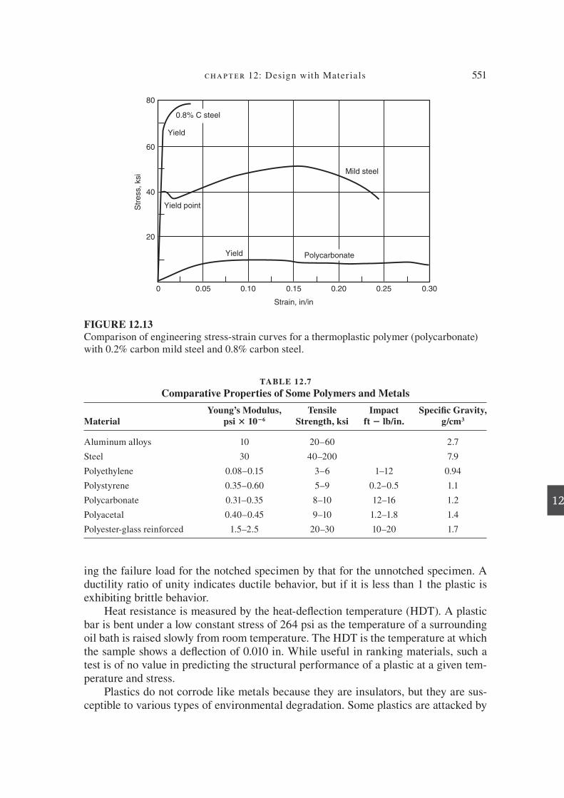
chapter 12: Design with Mater ia ls 551
12
ing the failure load for the notched specimen by that for the unnotched specimen. A ductility ratio of unity indicates ductile behavior, but if it is less than 1 the plastic is exhibiting brittle behavior.
Heat resistance is measured by the heat-del ection temperature (HDT). A plastic bar is bent under a low constant stress of 264 psi as the temperature of a surrounding oil bath is raised slowly from room temperature. The HDT is the temperature at which the sample shows a del ection of 0.010 in. While useful in ranking materials, such a test is of no value in predicting the structural performance of a plastic at a given tem-perature and stress.
Plastics do not corrode like metals because they are insulators, but they are sus-ceptible to various types of environmental degradation. Some plastics are attacked by
FIGURE 12.13
Comparison of engineering stress-strain curves for a thermoplastic polymer (polycarbonate) with 0.2% carbon mild steel and 0.8% carbon steel.
Yield
Yield pointStr
ess,
ksi
Yield
Mild steel
Polycarbonate
0.8% C steel
0 0.05
20
40
60
80
0.10 0.15
Strain, in/in
0.20 0.25 0.30
TABLE 12 .7
Comparative Properties of Some Polymers and Metals
Material
Young’s Modulus,
psi 3 10 6
Tensile
Strength, ksi
Impact
ft lb/in.
SpeciC c Gravity,
g/cm 3
Aluminum alloys 10 20–60 2.7
Steel 30 40–200 7.9
Polyethylene 0.08–0.15 3–6 1–12 0.94
Polystyrene 0.35–0.60 5–9 0.2–0.5 1.1
Polycarbonate 0.31–0.35 8–10 12–16 1.2
Polyacetal 0.40–0.45 9–10 1.2–1.8 1.4
Polyester-glass reinforced 1.5–2.5 20–30 10–20 1.7
die37039_ch12.indd 551 2/25/08 6:59:08 PM

552 engineering design
12
organic solvents and gasoline. Some are highly susceptible to the absorption of wa-ter vapor, which degrades mechanical properties and causes swelling. Many plastics are affected by ultraviolet radiation, causing cracking, fading of the color, or loss of transparency.
Many additives are compounded with the polymer to improve its properties. Fill-ers like wood l our, silica l our, or P ne clay are sometimes added as extenders to de-crease the volume of plastic resin used, and therefore the cost, without severely de-grading properties. Chopped glass P ber is commonly added to increase the stiffness and strength of plastics. Plasticizers are used to enhance l exibility and melt l ow dur-ing processing. Flame retardants are added to reduce the l ammability of plastics, but some of these are proving to be toxic. Colorants such as pigments and dyes are used to impart color. Ultraviolet light absorbers are used to stabilize the color and lengthen the life of the product when exposed to sunlight. Antistatic agents are used to reduce the buildup of electrostatic charges on an insulating plastic surface.
A category of plastics that is growing in importance as a material for engineered structures is plastic matrix composite materials . In these materials high-modulus, strong but often brittle P bers are embedded in a matrix of thermosetting plastic. 44 The P bers most often used are graphite or glass. Because of the high cost of materials and the complexity of fabrication, composite structures are used where a high premium is placed on lightweight, strong structures. Composite structures represent the ulti-mate in materials design in that the structure is laid up layer upon layer. Because the strength and stiffness reside in the P bers, and these are highly directional, great atten-tion must be paid to directional properties in the design.
12.6.2 Design for Stiffness
Young’s modulus is low for plastics when compared with metals, so resistance to de-l ection (stiffness) is often a concern regarding the use of plastics. The stiffness of a structure is dependent upon the elastic modulus of the material and the part geometry. For example, the maximum del ection of a cantilever beam of length L , loaded with a concentrated load P at its end, is
δmax
= =PL
EII
bhb
3 3
3 12where and is the beam width andd is its thickness.h (12.29)
Equation (12.29) shows that increasing the stiffness (i.e., reducing the del ection) can be achieved by either increasing the elastic modulus E or increasing the moment of inertia I , or both. Table 12.7 shows that the addition of short glass P bers to a nylon molding polymer can increase the elastic modulus. The addition of long glass P bers to an epoxy polymer matrix to make a composite material can increase the modulus much more, but at the complication of introducing extreme directionality (anisotropy) in properties.
44. ASM Handbook, Vol. 21, Composites, ASM International, Materials Park, OH , 2001 ; D . Hull , An
Introduction to Composite Materials, Cambridge University Press, Cambridge , 1981 ; R. J . Diefendorf , “Design with Composites,” ASM Handbook, Vol. 20, pp. 648–65 , 1997 .
die37039_ch12.indd 552 2/25/08 6:59:08 PM

chapter 12: Design with Mater ia ls 553
12
The second way to increase the stiffness of the cantilever beam is to increase the value of the moment of inertia, I . An obvious way to do this is to increase the value of the thickness h that appears in Eq. (12.29) raised to the third power. If a polymer has E 5 300,000 psi and a metal E 5 10,000,000 psi, the polymer beam will have to be more than three times thicker to have the same l exural rigidity as the aluminum beam. This introduces problems in addition to the extra cost of the additional mate-rial that must be used. Polymers have low thermal conductivity, so there are issues in cooling thick sections fast enough in production forming machines like injection molding. In fact, the limit on wall thickness is around 8 to 10 mm.
However, signiP cant increases in I can be achieved through modiP cation of the shape of the cross section to move material far away from the neutral axis. This is ex-pressed by the shape factor . The structural elements usually employed for this purpose are ribs or corrugation, Fig. 12.14. While corrugated surfaces provide greater stiffness, for equal weight and thickness, by a factor of about 1.8, they usually are avoided for aesthetic reasons and for the fact that they result in higher mold costs than do ribs. 45
In their simplest form, reinforcing ribs are beam-like structures. 46 Generally they are placed inside of the part attached to the load-bearing surface of a part and are oriented to run in the direction of maximum stress and del ection. As shown in Fig. 12.15, they can run the full length of the part or stop part way. When they do not intersect a vertical wall they should be tapered down gradually to aid in polymer melt l ow and to avoid stress concentration. A short rib used to support a wall is often called a gusset plate . The ribs should be tapered slightly (draft) to aid in ejection from the mold, and they should be designed with a generous radius where they attach to the plate to avoid stress concentration.
12.6.3 Time-Dependent Part Performance
The mechanical properties of plastics are viscoelastic . 47 This means that they vary with time under load, the rate of loading, and the temperature. This material behavior shows itself most prominently in the phenomena of creep and stress relaxation. Creep is the permanent deformation of a material over time, under constant load, and at con-
FIGURE 12.14
Examples of structural stiffening elements.
Rib Corrugation
45. G . Erhard , Designing with Plastics, Chap. 10, Hanser Gardner Publications, Cincinnati, OH , 2006 .
46. For a methodology with which to determine the value of I, see R. A . Malloy , Plastic Part Design for
Injection Molding, Hanser Gardner Publications, Cincinnati, OH , 1994 , pp. 213–30 . 47. J. G . Williams , Stress Analysis of Polymers, 2d ed., John Wiley-Halsted Press, New York , 1980 ; A.S . Wineman and K. R . Rajagopal , Mechanical Response of Polymers, Cambridge University Press, New York , 2000 .
die37039_ch12.indd 553 2/25/08 6:59:08 PM

554 engineering design
12
stant temperature. Stress relaxation measures the decreasing stress required to cause a constant strain at a constant temperature. For example, the loosening of a snap P t with time, or the loosening of a self-tapping screw, is a result of stress relaxation.
The calculation of stress and strain from viscoelastic equations that describe the creep of plastics is an advanced topic. However, design engineers have developed use-ful and simpler methods for designing with plastics. The procedure is as follows:
Determine the maximum service temperature and the time for which a constant load will be applied.
Calculate the maximum stress in the design using normal mechanics of material equations.
From a creep curve of strain versus time, P nd the strain from the appropriate tem-perature and stress.
Divide these values of strain into stress to determine an apparent creep modulus . This creep modulus can be used in mechanics of materials equations to determine deformation or del ection.
E X A M P L E 1 2 . 5 Design for Creep of Plastics
A simple beam of polyethylene terephthalate (PET) reinforced with 30 volume percent of short glass P bers is statically loaded with 10 lb in the middle of the beam. The beam is 8 in. long, 1 in. thick, and has a moment of inertia of I 5 0.0025 in. 4 For a beam loaded at midspan the bending moment is
MPL= = =4
10 8
420
3in. lb
The bending stress at the center of the beam at its outer P ber is
σ = = × =Mc
I
20 0 5
0 00254000
.
.psi
Figure 12.16 shows the l exural creep curves (log-log plot) for 30 percent GF PET. Since we are interested in long-term behavior, we look for the creep strain at 1000 h with the
●
●
●
●
●
FIGURE 12.15
Typical rib designs used to increase the stiffness of an injection molded plate.
RibsGusset plate
Partial
rib
Load 5 bearing surface
die37039_ch12.indd 554 2/25/08 6:59:09 PM
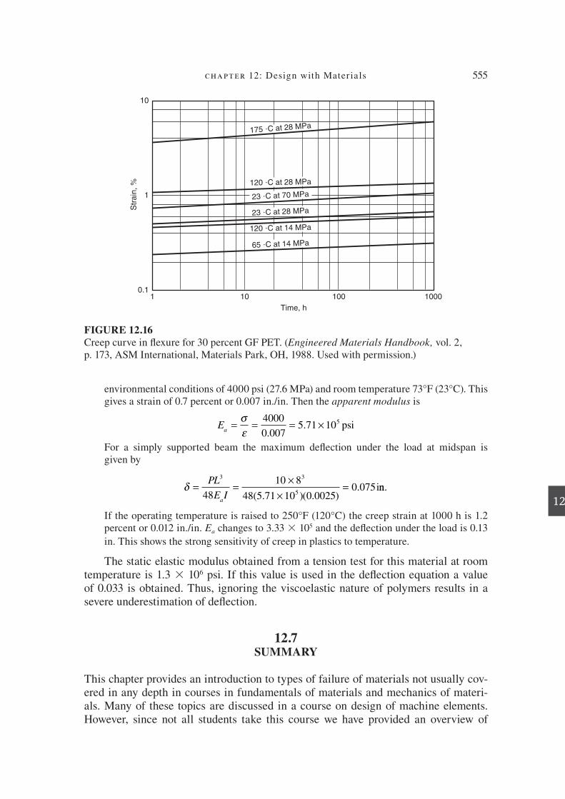
chapter 12: Design with Mater ia ls 555
12
environmental conditions of 4000 psi (27.6 MPa) and room temperature 73°F (23°C). This gives a strain of 0.7 percent or 0.007 in./in. Then the apparent modulus is
Ea
= = = ×σε
4000
0 0075 71 105
.. psi
For a simply supported beam the maximum del ection under the load at midspan isgiven by
δ = = ××
=PL
E Ia
3 3
548
10 8
48 5 71 10 0 00250 075
( . )( . ). inn.
If the operating temperature is raised to 250°F (120°C) the creep strain at 1000 h is 1.2 percent or 0.012 in./in. E a changes to 3.33 3 10 5 and the del ection under the load is 0.13
in. This shows the strong sensitivity of creep in plastics to temperature.
The static elastic modulus obtained from a tension test for this material at room temperature is 1.3 3 10 6 psi. If this value is used in the del ection equation a value of 0.033 is obtained. Thus, ignoring the viscoelastic nature of polymers results in a severe underestimation of del ection.
12.7 SUMMARY
This chapter provides an introduction to types of failure of materials not usually cov-ered in any depth in courses in fundamentals of materials and mechanics of materi-als. Many of these topics are discussed in a course on design of machine elements. However, since not all students take this course we have provided an overview of
FIGURE 12.16
Creep curve in l exure for 30 percent GF PET. ( Engineered Materials Handbook, vol. 2,p. 173, ASM International, Materials Park, OH, 1988. Used with permission.)
100.1
1
10
Str
ain
, %
1 100
Time, h
65 ?C at 14 MPa
120 ?C at 14 MPa
23 ?C at 28 MPa
23 ?C at 70 MPa
120 ?C at 28 MPa
175 ?C at 28 MPa
1000
die37039_ch12.indd 555 2/25/08 6:59:09 PM

556 engineering design
12
methods for design against the most common ways that machine elements fail. The approach is at a rather elementary level and does not consider failure in situations of combined stress. Ample references are given to sources where the student can extend their knowledge. The excellent text by Norman Dowling should be particularly help-ful, as will be the various volumes of the ASM Handbook that are referenced.
NEW TERMS AND CONCEPTS
Abrasive wear Endurance limit Notch sensitivity factor Adhesive wear Failsafe design Plane-strain fracture toughness Apparent modulus Fatigue failure Stress corrosion fracture Creep failure Fracture mechanics Viscoelastic behavior Damage tolerant design Low-cycle fatigue Wear
BIBLIOGRAPHY
ASM Handbook, Vol. 19, Fatigue and Fracture, ASM International, Materials Park, OH , 1996 .
ASM Handbook, Vol. 20, Materials Selection and Design, ASM International, Materials Park, OH , 1997 .
Budynas, R. G., and J. K. Nisbett: Shigley’s Mechanical Engineering Design, 8th ed., McGraw-Hill, New York, 2008.
Derby , B ., D. A . Hills , and C . Ruiz : Materials for Engineering: A Fundamental Design Ap-
proach, John Wiley & Sons, New York , 1992 . Dieter , G. E .: Mechanical Metallurgy, 3d ed., McGraw-Hill, New York , 1986 . Dowling , N. E .: Mechanical Behavior of Materials, 3d ed., Prentice Hall, Englewood Cliffs,
NJ , 2006 . Edwards , K. S ., and R. B . McKee : Fundamentals of Mechanical Component Design, McGraw-
Hill, New York , 1991 . Jones , D. R. H .: Engineering Materials 3: Materials Failure Analysis, Pergamon Press,
Oxford , 1993 .
PROBLEMS AND EXERCISES
12.1 Compare steels A and B for the construction of a pressure vessel 30 in. inside diameter and 12 ft long. The pressure vessel must withstand an internal pressure of 5000 psi. Use a factor of safety of 2 on the yield strength. For each steel, determine (a) critical l aw size and (b) l aw size for a leak-before-break condition. This is the situation where the crack penetrates the wall thickness before brittle fracture occurs.
Steel Yield Strength, ksi KIc, ksi in.
A 260 80
B 110 170
die37039_ch12.indd 556 2/25/08 6:59:09 PM

chapter 12: Design with Mater ia ls 557
12
12.2 A high-strength steel has a yield strength of 100 ksi and a fracture toughness . By the use of a certain nondestructive evaluation technique, the smallest-size l aw that can be de-tected routinely is 0.3 in. Assume that the most dangerous crack geometry in the structure
is a single-edge notch so that KIc
= 150 ksi in. The structure is subjected to cyclic
fatigue loading in which s max 5 45 ksi and s min 5 25 ksi. The crack growth rate for the steel is given by da / dN 5 0.66 3 10 28 (∆ K ) 2.25 . Estimate the number of cycles of fatigue stress that the structure can withstand.
12.3 A 3-inch-diameter steel shaft is rotating under a steady bending load. The shaft is re-duced in diameter at each end to P t in the bearings, which gives a theoretical stress concentration factor at this radius of 1.7. The fatigue limit of the steel in a rotating beam test is 48,000 psi. Its fatigue notch sensitivity factor is 0.8. Since the fatigue limit is close to a 50 percent survivability value, we want to design this beam to a 99 percent reliability. What point in the beam will be the likely point for a failure, and what is the maximum allowable stress at that point?
12.4 A 1.50-inch-diameter steel bar is subjected to a cyclical axial load of P max 5 75,000 lb in tension and 25,000 lb in compression. The fatigue limit (endurance limit) for a stress cycle with R 5 21.0 is 75 ksi. The ultimate tensile strength is 158 ksi and the yield strength is 147 ksi.
(a) Equation (12.16) expresses the relationship between alternating stress and the mean stress in fatigue known as the Goodman line. Plot Eq. (12.6) on coordinates of s a (y-axis) versus s m (x-axis) and label the critical points on this graph.
(b) To what value would the endurance limit be reduced by the stress cycle given here?
12.5 A high-carbon steel is used to make a leaf spring for a truck. The service loads the truck will experience can be approximated by an alternating stress from a maximum load to a zero load in tension ( R 5 0). In the heat-treated condition the leaf spring has a fatigue limit of 380 MPa based on laboratory tests made under completely reversed fatigue loading. The surface P nish of the leaf spring is expected to reduce this value by 20 percent. The ultimate tensile strength of the steel is 1450 MPa. Before assembly the leaf spring is shotpeened to introduce a surface compressive residual stress that is estimated to be 450 MPa. Find the maximum stress amplitude that the surface of the spring could be expected to withstand for an inP nite number of fatigue cycles.
12.6 A blastic beam (6 in. diameter) used to haul small loads into a loft extends 8 ft in the horizontal plane from the building. If the beam is made from glass-reinforced PET, how much would the beam del ect on a 23°C day when hauling up a 900 lb load?
12.7 Stress-corrosion failures that occur in the 304 and 316 stainless-steel recirculation pip-ing have been a major problem with boiling-water nuclear reactors (BWR). What are the three conditions necessary for stress-corrosion cracking? Suggest remedies for the cracking.
12.8 What are the chief advantages and disadvantages of plastic gears? Discuss how material structure and processing are utilized to improve performance.
die37039_ch12.indd 557 2/25/08 6:59:10 PM
13
13
DESIGN FOR MANUFACTURING
13.1
ROLE OF MANUFACTURING IN DESIGN
Producing the design is a critical link in the chain of events that starts with a creative idea and ends with a successful product in the marketplace. With modern technology the function of production no longer is a mundane activity. Rather, design, materials selection, and processing are inseparable, as shown in Fig. 11.1.
There is confusion of terminology concerning the engineering function called manufacturing . Materials engineers use the term materials processing to refer to the conversion of semi? nished products, like steel blooms or billets, into ? nished products, like cold-rolled sheet or hot-rolled bar. A mechanical, industrial, or manu-facturing engineer is more likely to refer to the conversion of the sheet into an au-tomotive body panel as manufacturing . Processing is the more generic term, but manufacturing is the more common term. Production engineering is a term used in Europe to describe what we call manufacturing in the United States. We will use the term manufacturing in this text to refer to converting a design into a ? nished product.
The ? rst half of the 20th century saw the maturation of manufacturing opera-tions in the western world. Increases in the scale and speed of operations brought about increases in productivity, and manufacturing costs dropped while wages and the standard of living rose. There was a great proliferation of available materials as basic substances were tailor-made to have selectively improved properties. One of the major achievements of this era was the development of the production line for mass-producing automobiles, appliances, and other consumer goods. Because of the preeminence in manufacturing that developed in the United States, there has been a recent tendency to take the production function for granted. Manufacturing has been downplayed in the education of engineers. Manufacturing positions in indus-try have been considered routine and not challenging, and as a result they have not
558
die37039_ch13.indd 558 2/25/08 6:59:37 PM
chapter 13: Design for Manufactur ing 559
13
attracted their share of the most talented engineering graduates. Fortunately, this situ-ation is improving as the rapid rise of manufacturing in Asia has threatened jobs for a large segment of the workforce in the western world. The nature and perception of manufacturing is being changed by increasing automation and computer-aided manufacturing.
Peter Drucker, the prominent social scientist and management expert, has termed the current manufacturing situation “the third industrial revolution.” The use of power, whether generated by falling water or a steam engine, determined the ? rst industrial revolution. The second industrial revolution began roughly a century ago when machines were ? rst driven directly by fractional-horsepower motors. Before machines were direct-driven by electric motors, they were driven by belts and pul-leys, which meant that the equipment had to be very close to the source of power. Thus, the second industrial revolution brought [ exibility and economy to manu-facturing. The third industrial revolution combines information processing capa-bilities with machines and tools. It is converting production into a knowledge-based operation.
A serious problem facing manufacturing companies has been the tendency to separate the design and manufacturing functions into different organizational units. Barriers between design and manufacturing decision making can inhibit the close interaction that the two engineering functions should have, as discussed previously under concurrent engineering (Sec. 2.4.4). When technology is sophisticated and fast-changing, a close partnership between the people in research, design, and manufactur-ing is very necessary.
That has been demonstrated best in the area of solid-state electronic devices. As semiconductor devices replaced vacuum tubes, it became apparent that design and processing could no longer be independent and separable functions. Design using vacuum-tube technology was essentially a linear process in which specialists in materi-als passed on their input to specialists in components who passed on their input to circuit designers who, in turn, communicated with system designers. With the advent of tran-sistors, the materials, device construction, and circuit design functions became closely coupled. Then, with the microelectronics revolution of large-scale integrated circuits, the entire operation from materials to system design became interwoven, and manu-facturing became inseparable from design. The result was a situation of rapid techni-cal advance requiring engineers of great creativity, [ exibility, and breadth. The payoff in making the personal computer and workstations a reality has been huge. Never has productivity been enhanced as rapidly as during the microelectronics revolution. This should serve as a model of the great payoff that can be achieved by closer integration of research, design, and manufacturing.
The need to break down barriers between design and manufacturing is widely recognized today and is accomplished by the use of concurrent engineering and the involvement of manufacturing engineers in product design and development teams. Also, focus on improving the link between manufacturing and design has increased emphasis on codifying a set of practices that designers should follow to make their designs easier to manufacture. This topic, design for manufacture (DFM), is the em-phasis of this chapter.
die37039_ch13.indd 559 2/25/08 6:59:38 PM

560 engineering design
13
13.2
MANUFACTURING FUNCTIONS
More conventional manufacturing is divided into the following functions: (1) process engineering, (2) tool engineering, (3) work standards, (4) plant engineering, and (5) administration and control. Process engineering is the development of a step-by-step sequence of operations for production. The overall product is subdivided into its com-ponents and subassemblies, and the steps required to produce each component are arranged in logical sequence. An important part of process engineering is to specify the related tooling. Vital parameters in process engineering are the rate of production and the cost of manufacturing a component. Tool engineering is concerned with the design of tools, jigs, > xtures, and gages to produce the part. Jigs both hold the part and guide the tool during manufacture, while ! xtures hold a part to be joined, assem-bled, or machined. Tools do the machining or forming, gages determine whether the dimensions of the part are within speci> cation. Work standards are time values as-sociated with each manufacturing operation that are used to determine standard costs to make the part. Other standards that need to be developed in manufacturing are tool standards and materials standards. Plant engineering is concerned with providing the plant facilities (space, utilities, transportation, storage, etc.) needed to carry out the manufacturing process. Administration and control deals with production planning, scheduling, and supervising to assure that materials, machines, tools, and people are available at the right time and in the quantities needed to produce the part.
During the last century modern manufacturing was typi> ed by the automotive assembly line. Now mass production manufacturing systems account for less than 25 percent of components manufactured. In fact, 75 percent of the parts manufactured are produced in lots of fewer than 50 pieces. About 40 percent of the employment in manufacturing is in such job-shop operations. Studies of batch-type metal-cutting production shops have shown that, on the average, a workpiece in such a shop is on a machine tool being productively processed only 5 percent of the time. Ninety-> ve percent of the time the workpiece is in the shop, it is waiting in an inventory of un> n-ished parts. Moreover, of the very small fraction of time the part is being worked on, it is being cut by the tool only about 30 percent of the time. The remaining 70 percent of the time is taken up by loading and unloading, positioning the workpiece, gaging the part, and other activities. Thus, there is a major opportunity for greatly increasing manufacturing productivity in small-lot manufacture.
Computer-automated machine tool systems, which include industrial robots and computer software for scheduling and inventory control, have demonstrated the abil-ity to increase machine utilization time from an average of 5 percent to as much as 90 percent. The introduction of computer-controlled machining centers that can perform many operations in a single machine greatly increases the productivity of the machine tool. The computer-automated factory—in which all steps in part manufacturing will be optimized by computer software systems, the machine tools will be under com-puter control, and at least half of the machines will be part of a versatile manufactur-ing system that features multiple machining capability and automatic parts handling between workstations—has been demonstrated at many plant sites. This automated factory differs from the automotive transfer line in that it is a R exible manufacturing
die37039_ch13.indd 560 2/25/08 6:59:38 PM

chapter 13: Design for Manufactur ing 561
13
system capable of producing a wide variety of parts under computer control. This broad-based effort throughout industry to link computers into all aspects of manufac-
turing is called computer-integrated manufacturing (CIM). Figure 13.1 shows the broad spectrum of activities that are encompassed by man-
ufacturing. It begins in step 4, when design engineering turns the complete informa-tion for the design over to the process planners. As mentioned earlier, many tasks of process planning are done concurrently with the detail design phase. Process selection and design of tooling are major functions in this step. Step 5 involves > ne-tuning a process, often by computer modeling or optimization processes, to improve through-put or improve yield (reduce defects) or decrease cost. Actual part manufacturing, step 6, involves production team training and motivation. In many instances a consider-able amount of materials handling is required. The many issues involved with step 7 are vital for an effective manufacturing operation. Finally, in step 8, the product is shipped and sold to the customer. Customer service, step 9, handles warranty and re-pair issues, and eventually the product is retired from service, hopefully by recycling.
4 Process planning
group technology
process selection
process design
process parameters
tools and dies
parts programming
jigs and fixtures
quality control
5 Process R & D
process choice
optimization
modeling
environmental etc.
considerations
6 Processing
parts manufacturing
sensing and corrective action
storing, moving, handling:
materials
parts
tooling
jigs and fixtures
assembly
7
CA
DCAM
Production control
routing
scheduling
production tracking
machine load monitoring
inventory:
parts
materials
in-process
purchasing
receiving
maintenance
quality assurance
standards
inspection
stat. proc. contr.
3 Production preparation
assembly drawings
part drawings
make/buy decisions
bill of materials
2 Product design
industrial design
mechanical
electrical
materials
product R & D
design
and
analysis
1 Sales (order processing)
Product concept
Market forecast
Market research
9 Customer
service
10 Recycling
Disposal
8
COMMON
DATABASE
FOR CIM
MR
P
Shipping
inventory
invoicing
accounting
FIGURE 13.1Spectrum of activities that are encompassed by manufacturing.
die37039_ch13.indd 561 2/25/08 6:59:38 PM

562 engineering design
13
The information gathered from customer service operations is fed back into the design of new products, step 2; the cycle is completed.
13.3 CLASSIFICATION OF MANUFACTURING PROCESSES
It is not an easy task to classify the tremendous variety of manufacturing processes. We start with the hierarchical classi> cation of business and industry shown in Fig. 13.2. The service industries consist of enterprises, such as education, banking, insurance, communication, and health care that provide important services to mod-ern society but do not create wealth by converting raw materials. The producing in-dustries acquire raw materials (minerals, natural products, or petroleum) and process them, through the use of energy, machinery, and brainpower, into products that serve the needs of society. The distribution industries, such as merchandising and transpor-tation, make those products available to the general public.
A characteristic of modern industrialized society is that an increasingly smaller percentage of the population produces the wealth that makes our afR uent society pos-sible. Just as the past century saw the United States change from a predominantly agrarian society to a nation in which only 3 percent of the population works in ag-riculture, so we are becoming a nation in which an ever-decreasing percentage of the workforce is engaged in manufacturing. In 1947 about 30 percent of the work-force was in manufacturing; in 1980 it was about 22 percent. By the year 2004 about 15 percent of U.S. workers were engaged in manufacturing.
The producing industries can be divided conveniently into raw materials produc-ers (mining, petroleum, agriculture), producers of discrete products (autos, consumer electronics, etc.), and industries engaged in continuous processing (gasoline, paper, steel, chemicals, etc.). Two major divisions of discrete products are construction (buildings, roads, bridges, etc.) and manufacturing. Under manufacturing we recog-nize batch (low-volume) manufacturing and mass production as categories.
Business and industry
Producing industryService industry Distribution industry
Discrete productsRaw materials Continuous processing
Construction Manufacturing
Batch manufacturing Mass production
FIGURE 13.2A simple hierarchical classi> cation of business and industry.
die37039_ch13.indd 562 2/25/08 6:59:38 PM

chapter 13: Design for Manufactur ing 563
13
13.3.1 Types of Manufacturing Processes
A manufacturing process converts a material into a > nished part or product. The changes that take place occur with respect to part geometry, or they can affect the internal microstructure and therefore the properties of the material. For example, a sheet of brass that is being drawn into the cylindrical shape of a cartridge case is also being hardened and reduced in ductility by the process of dislocation glide on slip planes.
Recall from Chap. 6 that the functional decomposition of a design was described initially in terms of energy, material, and information R ows. These same three factors are present in manufacturing. Thus, a manufacturing process requires an energy R ow to cause the material R ow that brings about changes in shape. The information R ow, which consists of both shape and material property information, depends on the type of material, the process used—that is, whether mechanical, chemical, or thermal—the characteristics of the tooling used, and the pattern of movement of the material rela-tive to the tooling.
A natural division among the hundreds of manufacturing processes is whether the process is mass conserving or mass reducing . In a mass conserving process the mass of the starting material is approximately equal to the mass of the > nal part. Most processes are of this type. A shape replication process is a mass conserving process in which the part replicates the information stored in the tooling by being forced to assume the shape of the surface of the tool cavity. Casting, injection molding, and closed-die forging are examples. In a mass reducing process, the mass of the starting material is greater than the mass of the > nal part. Such processes are shape-genera-
tion processes because the part shape is produced by the relative motion between the tool and the workpiece. Material removal is caused by controlled fracture, melting, or chemical reaction. A machining process, such as milling, is an example of controlled fracture.
A different way of dividing manufacturing processes is to classify them into three broad families: (1) primary processes, (2) secondary processes, and (3) > nishing processes.
Primary processes take raw materials and create a shape. The chief categories are casting processes, polymer processing or molding processes, deformation pro-cesses, and powder processes.
Secondary processes modify shape by adding features such as keyways, screw threads, and grooves. Machining processes are the main type of secondary pro-cesses. Other important categories are joining processes that fasten parts together, and heat treatment to change mechanical properties.
Finishing processes produce the > nal appearance and feel of a product by pro-cesses such as coating, painting, or polishing.
The taxonomy structure used to classify materials in Sec. 11.2.1 can be applied to manufacturing processes. For example, the Family of Shaping Processes can be divided into the Classes of Casting, Polymer Molding, Deformation, and Powder pro-cesses. The class Deformation Processes can, in turn, be broken into many Member processes such as rolling, drawing, cold forming, swaging, sheet metal forming, and
●
●
●
die37039_ch13.indd 563 2/25/08 6:59:39 PM

564 engineering design
13
spinning. Then, for each process we would need to determine Attributes or process
characteristics (PC) such as its applicability to certain ranges of part size, the mini-mum thickness that can be consistently produced by the process, the typical tolerance on dimensions and surface roughness produced by the process, and its economical batch size.
13.3.2 Brief Description of the Classes of Manufacturing Processes
This section provides further understanding of the major classes of manufacturing processes. 1
Casting (solidi> cation) processes: Molten liquid is poured into a mold and solidi-> ed into a shape de> ned by the contours of the mold. The liquid > lls the mold by R ow under its own weight or with a modest pressure. Cast shapes are designed so the liquid R ows to all parts of the mold cavity, and solidi> cation occurs progres-sively so there are no trapped liquid pockets in a solidi> ed shell. This requires a low-viscosity liquid, so casting is usually done with metals and their alloys. The various casting processes, and their costs differ chieR y according to the expense and care used to prepare the mold. Great progress has been made using computer models to predict and control the R ow and solidi> cation of the liquid material, thereby minimizing casting defects. Polymer processing (molding): The wide use of polymers has brought about the de-velopment of processes tailored to their high viscosity. In most of these processes a hot viscous polymer is either compressed or injected into a mold. The distinc-tion between casting and molding is the viscosity of the material being worked. Molding can take such extreme forms as compression molding plastic pellets in a hot mold, or blowing a plastic tube into the shape of a milk bottle against a mold wall. Deformation processes: A material, usually metal, is plastically deformed hot or cold to give it improved properties and change its shape. Deformation processes are also called metal-forming processes. Typical processes of this type are forging, rolling, extrusion, and wire drawing. Sheet-metal forming is a special category in which the deformation occurs in a two-dimensional stress state instead of three dimensions. Powder processing: This rapidly developing manufacturing area involves the con-solidation of particles of metal, ceramics, or polymers by pressing and sintering, hot compaction, or plastic deformation. It also includes the processing of compos-ite materials. Powder metallurgy is used to make small parts with precision dimen-sions that require no machining or > nishing. Powder processing is the best route for materials that cannot be cast or deformed, such as very high melting point met-als and ceramics.
1.
2.
3.
4.
1. A six-page taxonomy of manufacturing processes leading to many illustrated descriptions of processes is given at http://en.wikipedia.org/wiki/Taxonomy_of_manufacturing_processes. Also see http://www.designsite.dk/Processes. Accessed January 7, 2007.
die37039_ch13.indd 564 2/25/08 6:59:39 PM
chapter 13: Design for Manufactur ing 565
13
Material removal or cutting (machining) processes: Material is removed from a workpiece with a hard, sharp tool by a variety of methods such as turning, milling, grinding, and shaving. Material removal occurs by controlled fracture, produc-ing chips. Machining is one of the oldest manufacturing processes, dating back to the invention of the power lathe early in the Industrial Revolution. Essentially any shape can be produced by a series of machining operations. Because a machining operation starts with a manufactured shape, such as bar stock, casting, or forging, it is classi> ed as a secondary process. Joining processing: Included in joining processing are all categories of welding, brazing, soldering, diffusion bonding, riveting, bolting, and adhesive bonding. These operations attach the parts to one another. Fastening occurs in the assembly step of manufacturing. Heat treatment and surface treatment: This category includes the improvement of mechanical properties by thermal heat treatment processes as well as the im-provement of surface properties by diffusion processes like carburizing and ni-triding or by alternative means such as sprayed or hot-dip coatings, electroplat-ing, and painting. The category also includes the cleaning of surfaces preparatory to surface treatment. This class of processes can be either secondary or > nishing processes. Assembly processes: In this, usually the > nal step in manufacturing, a number of parts are brought together and combined into a subassembly or > nished product.
13.3.3 Sources of Information on Manufacturing Processes
In this book we cannot describe the many processes used in modern manufacturing in detail. Table 13.1 lists several readily available texts that describe the behavior of the material, the machinery, and the tooling to present a good understanding of how each process works.
13.3.4 Types of Manufacturing Systems
There are four general types of manufacturing systems: job shop, batch, assembly line, and continuous R ow. 2 The characteristics of these production systems are listed in Table 13.2. The job shop is characterized by small batches of a large number of dif-ferent part types every year. There is no regular work R ow, so work-in-process must often wait in a queue for its turn on the machine. Hence, it is dif> cult to specify job shop capacity because it is highly dependent on the product mix. Batch " ow , or de-coupled R ow line, is used when the product design is relatively stable and produced in periodic batches, but the volume for an individual product is not suf> cient to warrant the cost of specialized, dedicated equipment. Examples are the production of heavy equipment or ready-to-wear clothing. With assembly-line production, the equipment
5.
6.
7.
8.
2. G . Chryssolouris , Manufacturing Systems, 2d ed., Springer, New York , 2006 .
die37039_ch13.indd 565 2/25/08 6:59:39 PM

566 engineering design
13
TABLE 13.1
Basic Texts on Manufacturing Processes
DeGarmo, E. P., J. T. Black, and R. Kohser, Materials and Processes in Manufacturing, 9th ed., John Wiley & Sons, New York, 2003.
Groover, M. P., Fundamentals of Modern Manufacturing, 2d ed., John Wiley & Sons, New York, 2002.
Kalpakjian, S., and S. R. Schmid, Manufacturing Engineering and Technology, 5th ed., Pearson Pren-tice Hall, Upper Saddle River, NJ, 2006.
Schey, J. A., Introduction to Manufacturing Processes, 3d ed., McGraw-Hill, New York, 2000.
Also, Section 7, Manufacturing Aspects of Design, in ASM Handbook Vol. 20 gives an overview of each major process from the viewpoint of the design engineer.
The most important reference sources giving information on industrial practices are Tool and Manu-
facturing Engineers Handbook, 4th ed., published in nine volumes by the Society of Manufacturing Engineers, and various volumes of ASM Handbook published by ASM International devoted to spe-ci> c manufacturing processes, see Table 13.5. More books dealing with each of the eight classes of manufacturing processes are listed below. Most of these books give more advanced treatments than the texts listed in Table 13.1.
Casting Processes
M. Blair and T. L. Stevens, eds., Steel Castings Handbook, 6th ed., ASM International, Materials Park, OH, 1995.
J. Campbell, Casting, Butterworth-Heinemann, Oxford, UK, 1991.
H. Fredriksson and U. Åkerlind, Material Processing During Casting, John Wiley & Sons, Chichester, UK, 2006.
S. P. Thomas, ed., Design and Procurement of High-Strength Structural Aluminum Castings, American Foundrymen’s Society, Cleveland, 1995.
Casting, ASM Handbook, Vol. 15, ASM International, Materials Park, OH, 1988.
Polymer Processing
E. A. Muccio, Plastics Processing Technology, ASM International, Materials Park, OH, 1994.
A. B. Strong, Plastics: Materials and Processing, 3d ed., Prentice Hall, Upper Saddle River, NJ, 2006.
Plastics Parts Manufacturing, Tool and Manufacturing Engineers Handbook, Vol. 8, 4th ed., Society of Manufacturing Engineers, Dearborn, MI, 1995.
J. F. Agassant, P. Avenas, J. Sergent, and P. J. Carreau, Polymer Processing: Principles and Modeling, Hanser Gardner Publications, Cincinnati, OH 1991.
Z. Tadmor and C. G. Gogas, Principles of Polymer Processing, 2d ed., Wiley-Interscience, Hoboken, NJ, 2006.
Deformation Processes
W. A. Backofen, Deformation Processing, Addison-Wesley, Reading, MA, 1972.
W. F. Hosfortd and R. M. Caddell, Metal Forming: Mechanics and Metallurgy, 2d ed., Prentice Hall, Upper Saddle River, NJ, 1993.
E. Mielnik, Metalworking Science and Engineering, McGraw-Hill, New York, 1991.
R. H. Wagoner and J-L Chenot, Metal Forming Analysis, Cambridge University Press, Cambridge, UK, 2001.
K. Lange, ed., Handbook of Metal Forming, Society of Manufacturing Engineers, Dearborn, MI, 1985.
R. Pearce, Sheet Metal Forming, Adam Hilger, Bristol, UK, 1991.
Metalworking: Bulk Forming, ASM Handbook, Vol. 14A, ASM International, Materials Park, OH 2005.
Metalworking: Sheet Forming. ASM Handbook, Vol. 14B, ASM International, Materials Park, OH 2006.
die37039_ch13.indd 566 2/25/08 6:59:40 PM

chapter 13: Design for Manufactur ing 567
13
Z. Marciniak and J. L. Duncan, The Mechanics of Sheet Metal Forming, Edward Arnold, London, 1992.
Powder Processing
R. M. German, Powder Metallurgy Science, Metal Powder Industries Federation, Princeton, NJ, 1985.
R. M. German, Powder Metallurgy of Iron and Steel, John Wiley & Sons, New York, 1998.
ASM Handbook, Vol. 7, Powder Metal Technologies and Applications, ASM International, Materials Park, OH, 1998.
Powder Metallurgy Design Manual, 2d ed., Metal Powder Industries Federation, Princeton, NJ, 1995.
Material Removal Processes
G. Boothroyd and W. W. Knight, Fundamentals of Machining and Machine Tools, 3d ed., Taylor & Francis, Boca Raton, FL, 2006.
T. C. Childs, K. Maekowa, T. Objkawa, and T. Yamada, Metal Cutting Theory and Applications, John Wiley & Sons, New York, 2002.
W. R. DeVries, Analysis of Metal Removal Processes, Springer-Verlag, New York, 1992.
S. Malkin, Grinding Technology: Theory and Applications, Ellis Horwood, New York, 1989.
M. C. Shaw, Metal Cutting Principles, 4th ed., Oxford University Press, New York, 1984.
Machining, Tool and Manufacturing Engineers Handbook, Vol. 1, 4th ed., Society of Manufacturing Engineers, Dearborn, MI, 1983.
ASM Handbook, Vol. 16, Machining, ASM International, Materials Park, OH, 1989.
Joining Processes
S. Kuo, Welding Metallurgy, John Wiley & Sons, New York, 1987.
R. W. Messler, Principles of Welding, John Wiley and Sons, New York, 1999.
Engineered Materials Handbook, Vol. 3, Adhesives and Sealants, ASM International, Materials Park, OH, 1990.
R. O. Parmley, ed., Standard Handbook for Fastening and Joining, 3d ed., McGraw-Hill, New York, 1997.
ASM Handbook, Vol. 6, Welding, Brazing, and Soldering, ASM International, Materials Park, OH, 1993.
Welding Handbook, 9th ed., American Welding Society, Miami, FL, 2001.
Heat Treatment and Surface Treatment
Heat Treating, ASM Handbook, Vol. 4, ASM International, Materials Park, OH, 1991.
ASM Handbook, Vol. 5, Surface Engineering, ASM International, Materials Park, OH, 1994.
Tool and Manufacturing Engineers Handbook, Vol. 3, Materials, Finishing, and Coating, 4th ed., Soci-ety of Manufacturing Engineers, Dearborn, MI, 1985.
Assembly Processes
G. Boothroyd, Assembly Automation and Product Design, Marcel Dekker, New York, 1992.
E. K. Henriksen, Jig and Fixture Design, Industrial Press, New York, 1973.
P. H. Joshi, Jigs and Fixtures Design Manual, McGraw-Hill, New York, 2003.
A. H. Redford and J. Chal, Design for Assembly, McGraw-Hill, New York, 1994.
Fundamentals of Tool Design, 5th ed., Society of Manufacturing Engineers, Dearborn, MI, 2003.
Tool and Manufacturing Engineers Handbook, Vol. 9, Assembly Processes, 4th ed., Society of Manu-facturing Engineers, Dearborn, MI, 1998.
TABLE 13.1
(continued)
die37039_ch13.indd 567 2/25/08 6:59:40 PM

568 engineering design
13
is laid out in the sequence of usage. The large number of assembly tasks is divided into small subsets to be performed at successive workstations. Examples are the pro-duction of automobiles or power hand tools. Finally, a continuous-" ow process is the most specialized type. The equipment is highly specialized, laid out in a circuit, and usually automated. The material R ows continuously from input to output. Examples are a gasoline re> nery or a paper mill.
A process is said to be mechanized when it is being carried out by powered ma-chinery and not by hand. Nearly all manufacturing processes in developed countries are mechanized. A process is automated when the steps in the process, along with the movement of material and inspection of the parts, are automatically performed or controlled by self-operating devices. Automation involves mechanization plus sensing and controlling capabilities (programmable logic controllers and PCs). Hard automa-tion is hard-linked and hard-wired, while R exible automation includes the added capa-bility of being reprogrammed to meet changing conditions.
13.4 MANUFACTURING PROCESS SELECTION
The factors that inR uence the selection of a process to make a part are:
Quantity of parts required Complexity—shape, size, features Material
●
●
●
TABLE 13.2
Characteristics of Production Systems
Characteristic Job Shop Batch Flow Assembly Line Continuous Flow
Equipment and Physical Layout
Batch size Low (1–100 units)
Moderate (100–10,000 units)
Large (10,000–millions/year)
Large. Measured in tons, gals., etc.
Process R ow Few dominant R ow patterns
Some R ow patterns Rigid R ow patterns
Well de> ned and inR exible
Equipment General-purpose
Mixed Specialized Specialized
Setups Frequent Occasional Few and costly Rare and expensive
Process changes for new products
Incremental Often incremental Varies Often radical
Information and Control
Production informa-tion requirements
High Varies Moderate Low
Raw material inventory
Small Moderate Varies; frequent deliveries
Large
Work-in-process Large Moderate Small Very small
die37039_ch13.indd 568 2/25/08 6:59:40 PM

chapter 13: Design for Manufactur ing 569
13
Quality of part Cost to manufacture Availability, lead time, and delivery schedule
As emphasized in Chap. 11, there is a close interdependance between material selec-tion and process selection.
The steps in selecting a manufacturing process are:
Based on the part speci> cation, identify the material class, the required number of parts, and the size, shape, minimum thickness, surface > nish, and tolerance on critical dimensions of the part. These constitute constraints on the selection of the process.
Decide what the objective of the process selection process is. Generally, the objec-tive is to minimize the cost of the manufactured part. However, it might be to maxi-mize the quality of the part, or to minimize the time to make it.
Using the identi> ed constraints, screen a large number of processes to eliminate the processes incapable of meeting them. This can be done using the information sources given in this chapter, or the screening charts found in M. F. Ashby, Materi-
als Selection in Mechanical Design, 3d ed., Butterworth-Heinemann, Oxford, UK, 2005. The Cambridge Engineering Selector v. 4 software from Granta Design Ltd., Cambridge, UK, 2006 greatly facilitates this process. It links material selection with possible processes and provides extensive data about each process. Figure 13.3 shows an example of the information provided about a process.
Having narrowed the possible processes to a smaller number, they should be ranked based on manufacturing cost. A quick ranking can be based on the economic batch size (Sec. 13.4.1), but a cost model is needed (Sec. 13.4.6) for making the > nal decision. However, before making this decision it is important to seek supporting information from among the references given in Sec. 13.3.3 and elsewhere in this chapter. Look for case studies and examples of industry practice that will lend cred-ibility and support your decision.
Each factor affecting the selection of a manufacturing process for a particular part is discussed in the following sections.
13.4.1 Quantity of Parts Required
Two important factors in the choice of processes are the total number of parts to be produced and the rate of production, in units per time period. All manufacturing pro-cesses have a minimum number of pieces (volume) that must be made to justify their use. Some processes, like an automatic screw machine, are inherently high-volume processes, in that the setup time is long relative to the time needed to produce a single part. Others, like the hand layup of a > berglass plastic boat, are low-volume processes. Here the setup time is minimal but the time to make a part is much longer.
The total volume of production often is insuf> cient to keep a production machine continuously occupied. As a result, production occurs in batches or lots representing a fraction of the number of parts needed for a year of product production. The batch size is inR uenced by the cost and inconvenience of setting up for a new production run
●
●
●
●
●
●
●
die37039_ch13.indd 569 2/25/08 6:59:41 PM

13
570
FIGURE 13.3Typical process data sheet from CES EduPack, 2006 Granta Design Limited, Cambridge, UK, 2006.
Nozzle
Cylinder
Heater
Physical Attributes
Adjacent section ratio 1 2 2
Aspect ratio 1 2 250
Mass range 0.02205 2 55.12 lb
Minimum hole diameter 0.02362 2 in
Minimum corner radius 0.05906 2 in
Range of section thickness 0.01575 2 0.248 in.
Roughness 7.874e-3 2 0.06299 mil
Quality factor (1210) 1 2 6
Tolerance 3.937e-3 2 0.03937 in.
Econonic Attributes
Economic batch size (mass) 1.102e4 2 1.102e6 Ib
Economic batch size (units) 1e4 2 1e6
Cost Modelling
Relative cost index (per unit) 18.16 2 113.3
Capital cost 3.77e4 2 8.483e5 USD
Lead time 4 2 6 week(s)
Material utilization fraction 0.6 2 0.9
Production rate (mass) 66.14 2 2205 lb/hr
Production rate (units) 60 2 3000 /hr
Tool life (mass) 1.102e4 2 1.102e6 Ib
Tool life (units) 1e4 2 1e6
Supporting Information
Design guidelines
Complex shapes are possible. Thick sections or large changes in section are not
recommended. Small reentrant angles are possible.
Technical nodes
Most thermoplastics can be injection moulded. Some high melting point polymers (e.g.,
PTFE) are not suitable. Thermoplastic based composites (short fibre and particulate filled)
are also processed.
Injection-moulded parts are generally thin-walled.
Typical uses
Extremely varied. Housings, containers, covers, knobs, tool handles, plumbing fittings,
lenses, etc.
The economics
Tooling cost range covers small, simple to large, complex moulds. Production rate depends
on complexity of component and number of mould cavities.
The environment
Thermoplastic sprues can be recycled. Extraction may be required for volatile fumes.
Significant dust exposures may occur in the formulation of the resins. Thermostatic
controller malfunctions can be extremely hazardous.
Process Schematic
Screw
Granular PolymerMould
Parameters: Material Cost = 4.309USD/lb, component Mass 5 2.205lb, Batch size 5 1000,
INJECTION MOLDING of thermoplastics is the equivalent of pressure die casting of
metals. Molten polymer is injected under high pressure into a cold steel mold. The polymer
solidifies under pressure and the molding is then ejected.
Various types of injection molding machines exist, but the most common in use today is the
reciprocating screw machine (shown schematically). Capital and tooling costs are very high.
Production rate can be high, particularly for small moldings. Multicavity molds are often
used. The process is used almost exclusively for large-volume production. Prototype
moldings can be made using cheaper single-cavity molds of cheaper materials. Quality can
be high but may be traded off against production rate. The process may also be used with
thermosets and rubbers. Some modifications are required—this is dealt with separately.
Complex shapes are possible, though some features (e.g., undercuts, screw threads, inserts)
may result in increased tooling costs.
die37039_ch13.indd 570 2/25/08 6:59:41 PM
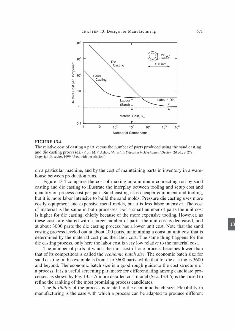
chapter 13: Design for Manufactur ing 571
13
on a particular machine, and by the cost of maintaining parts in inventory in a ware-house between production runs.
Figure 13.4 compares the cost of making an aluminum connecting rod by sand casting and die casting to illustrate the interplay between tooling and setup cost and quantity on process cost per part. Sand casting uses cheaper equipment and tooling, but it is more labor intensive to build the sand molds. Pressure die casting uses more costly equipment and expensive metal molds, but it is less labor intensive. The cost of material is the same in both processes. For a small number of parts the unit cost is higher for die casting, chieR y because of the more expensive tooling. However, as these costs are shared with a larger number of parts, the unit cost is decreased, and at about 3000 parts the die casting process has a lower unit cost. Note that the sand casting process leveled out at about 100 parts, maintaining a constant unit cost that is determined by the material cost plus the labor cost. The same thing happens for the die casting process, only here the labor cost is very low relative to the material cost.
The number of parts at which the unit cost of one process becomes lower than that of its competitors is called the economic batch size . The economic batch size for sand casting in this example is from 1 to 3600 parts, while that for die casting is 3600 and beyond. The economic batch size is a good rough guide to the cost structure of a process. It is a useful screening parameter for differentiating among candidate pro-cesses, as shown by Fig. 13.5. A more detailed cost model (Sec. 13.4.6) is then used to re> ne the ranking of the most promising process candidates.
The " exibility of the process is related to the economic batch size. Flexibility in manufacturing is the ease with which a process can be adapted to produce different
FIGURE 13.4 The relative cost of casting a part versus the number of parts produced using the sand casting and die casting processes. (From M. F . Ashby , Materials Selection in Mechanical Design , 2d ed., p. 278 , Copyright Elsevier, 1999 . Used with permission.)
Die
104
103
102
10
1
0.11 10 102 103 104 105 106
Sand
Casting 150 mm
Casting
Re
lative
Co
st
pe
r C
om
po
ne
nt
Labour
(Sand)
Labour (Die)
Material Cost, Cm
Number of Components
die37039_ch13.indd 571 2/25/08 6:59:41 PM
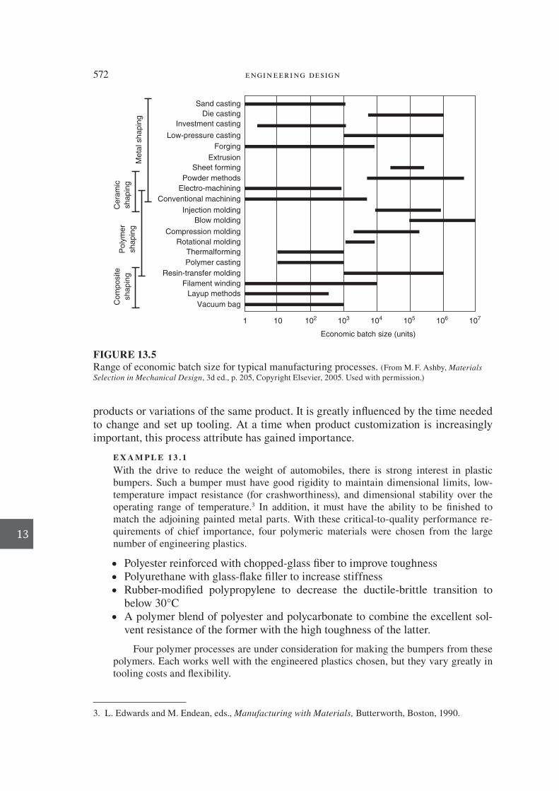
572 engineering design
13
products or variations of the same product. It is greatly inR uenced by the time needed to change and set up tooling. At a time when product customization is increasingly important, this process attribute has gained importance.
E X A M P L E 1 3 . 1
With the drive to reduce the weight of automobiles, there is strong interest in plastic bumpers. Such a bumper must have good rigidity to maintain dimensional limits, low- temperature impact resistance (for crashworthiness), and dimensional stability over the operating range of temperature. 3 In addition, it must have the ability to be > nished to match the adjoining painted metal parts. With these critical-to-quality performance re-quirements of chief importance, four polymeric materials were chosen from the large number of engineering plastics.
Polyester reinforced with chopped-glass > ber to improve toughness Polyurethane with glass-R ake > ller to increase stiffness Rubber-modi> ed polypropylene to decrease the ductile-brittle transition to
below 30°C A polymer blend of polyester and polycarbonate to combine the excellent sol-
vent resistance of the former with the high toughness of the latter.
Four polymer processes are under consideration for making the bumpers from these polymers. Each works well with the engineered plastics chosen, but they vary greatly in tooling costs and R exibility.
●
●
●
●
FIGURE 13.5Range of economic batch size for typical manufacturing processes. (From M. F. Ashby, Materials
Selection in Mechanical Design, 3d ed., p. 205, Copyright Elsevier, 2005. Used with permission.)
Sand casting
Die casting
Investment casting
Low-pressure casting
Forging
Extrusion
Sheet forming
Powder methods
Electro-machining
Conventional machining
Injection molding
Blow molding
Compression molding
Rotational molding
Thermalforming
Polymer casting
Resin-transfer molding
Filament winding
Layup methods
Vacuum bag
Economic batch size (units)
10 102 103 104 105 106 1071
Co
mp
osite
sh
ap
ing
Ce
ram
ic
sh
ap
ing
Po
lym
er
sh
ap
ing
Me
tal sh
ap
ing
3. L . Edwards and M . Endean , eds., Manufacturing with Materials, Butterworth, Boston , 1990 .
die37039_ch13.indd 572 2/25/08 6:59:42 PM

chapter 13: Design for Manufactur ing 573
13
Then, the part cost is the sum of the mold cost per part plus the labor input, neglecting the material cost, which is roughly the same for each.
Note how the unit part cost varies greatly with the quantity of parts required. The hand layup process of contact molding is the least expensive for a low part volume, while the low-cycle-time injection molding process excels at the highest part volume. Assuming that the material cost for the bumper is $30 per part, we see how material cost represents the largest fraction of the total cost as the part volume increases.
13.4.2 Shape and Feature Complexity
The complexity of a part refers to its shape and type and number of features that it contains. One way of expressing the complexity of a component is through its infor-mation content I, expressed in number of digital bits of information.
I nl
l=
∆
log2 (13.1)
where n 5 number of dimensions of the component
l l l l ln
n
=( )1 2 3
1• • ...
/is thegeometricmean dimenssion
is thegeometri∆ = ∆ ∆ ∆ ∆( )l l l l ln
n
1 2 3
1• • ...
/ccmeanof the tolerance
log2 xx( )=
( )(
log
log10
10 2)) Simple shapes contain only a few bits of information. Complex shapes, like integrated circuits, contain very many. A cast engine block might have 10 3 bits of information, but after machining the various features the complexity increases by both adding new dimensions ( n ) and improving their precision (reducing ∆l ).
Most mechanical parts have a three-dimensional shape, although sheet metal fab-rications are basically two-dimensional. Figure 13.6 shows a useful shape classi> ca-
Process Mold cost Labor input/unit
Injection molding $450,000 3 min 5 $1
Reaction injection molding $90,000 6 min 5 $2
Compression molding $55,000 6 min 5 $2
Contact molding $20,000 1 h 5 $20
Cost per part
Process 1000 parts 10,000 parts 100,000 parts 1,000,000 parts
Injection molding $451 $46 $5.50 $1.45
Reaction injection molding $92 $11 $2.90 $2.09
Compression molding $57 $7.50 $2.55 $2.06
Contact molding $40 $22 $20.20 $20.02
die37039_ch13.indd 573 2/25/08 6:59:42 PM

574 engineering design
13
tion system. In this schema a shape of uniform cross section is given a complexity rating of 0.
The shape complexity increases from left to right in Fig. 13.6 with the addition of greater geometric complexity and added features, that is, greater information content. Note that a small increase in information content can have major signi> cance in process selection for making a part. Moving from the solid shape R0 (shape in column 0 of the Round row) to the hollow shape T0 (shape in column 0 of the Tube row) adds only one additional dimension (the hole diameter), but the change excludes some processes as the best choice for making the part or adds an additional operation step in other processes.
Different manufacturing processes vary in their limitations for producing complex shapes. For example, there are many processes that do not allow the making of under-
cuts , shown in the bottom row in Fig. 13.6. Undercuts make it impossible to extract the part from the mold without complicated and expensive tooling. Other processes have limitations on how thin the wall thickness can be, or require the part to have uniform wall thickness. Extrusion processes require a part that is axially symmetric. Powder metallurgy cannot make parts with sharp corners or acute angles because the unsin-tered powder will crumble when transferring from the die. Lathe turning requires a part with cylindrical symmetry. Table 13.3 associates the shapes de> ned in Fig. 13.6 with the ability of various manufacturing processes to create them.
FIGURE 13.6A classi> cation system for basic shapes in design. (J. A. Schey, Introduction to Manufacturing
Processes, 3d ed. McGraw-Hill, 2000)
AbbreviationUniform
cross section
0Change at
end
1Change at
center
2Spatial
curve
3Closed
one end
4Closed
both ends
5Transverse
element
6Irregular
(complex)
7
R(ound)
B(ar)
S(ection, open)
SS(emiclosed)
T(ube)
F(lat)
Sp(herical)
U(ndercut)
Increasing spatial complexity
die37039_ch13.indd 574 2/25/08 6:59:42 PM

chapter 13: Design for Manufactur ing 575
13
TABLE 13.3
Ability of Manufacturing Processes to Produce Shapes in Fig. 13.6
Process Capability for producing shapes
Casting processes
Sand casting Can make all shapes
Plaster casting Can make all shapes
Investment casting Can make all shapes
Permanent mold Can make all shapes except T3, T5; F5; U1, U5, U7
Die casting Same as permanent mold casting
Deformation processes
Open-die forging Best for R0 to R3; all B shapes; T1; F0; Sp6
Hot impression die forging Best for all R, B, and S shapes; T1, T2; Sp
Hot extrusion All 0 shapes
Cold forging/ cold extrusion Same as hot die forging or extrusion
Shape drawing All 0 shapes
Shape rolling All 0 shapes
Sheet-metal working processes
Blanking F0 to F2; T7
Bending R3; B3; S0, S2, S7; T3; F3, F6,
Stretching F4; S7
Deep drawing T4; F4, F7
Spinning T1, T2, T4, T6; F4, F5
Polymer processes
Extrusion All 0 shapes
Injection molding Can make all shapes with proper coring
Compression molding All shapes except T3, T5, T6, F5, U4
Sheet thermoforming T4, F4, F7, S5
Powder metallurgy processes
Cold press and sinter All shapes except S3, T2, T3, T5, T6, F3, F5, all U shapes
Hot isostatic pressing All shapes except T5 and F5
Powder injection molding All shapes except T5, F5, U1, U4
PM forging Same shape restrictions as cold press and sinter
Machining processes
Lathe turning R0, R1, R2, R7; T0, T1, T2; Sp1, Sp6; U1, U2
Drilling T0, T6
Milling All B, S, SS shapes; F0 to F4; F6, F7, U7
Grinding Same as turning and milling
Honing, lapping R0 to R2; B0 to B2; B7; T0 to T2, T4 to T7; F0 to F2; Sp
Based on data from J.A. Schey, Introduction to Manufacturing Processes.
die37039_ch13.indd 575 2/25/08 6:59:43 PM

576 engineering design
13
13.4.3 Size
Parts vary considerably in size. Because of the nature of the equipment used in a manufacturing process, each process has a range of part sizes for which it is economi-cal to use that process. Figure 13.7 shows this.
Note that machining processes (i.e., removal of metal by cutting) span the com-plete range of sizes, and that machining, casting, and forging are able to produce the largest mass objects. However only a limited number of plants in the world can make very large parts. Therefore, to make very large products like aircraft, ships, and pres-sure vessels, it is necessary to assemble them from many parts using joining methods such as welding and riveting.
A limiting geometric factor in process selection often is section thickness. Figure 13.8 displays capabilities for achieving thickness according to process. Gravity-fed castings have a minimum wall thickness that they can produce due to surface ten-sion and heat R ow considerations. This can be extended by using pressure die casting. The availability of press tonnage and the occurrence of friction in metal deforma-tion processes create a similar restriction on minimum section thickness. In injec-
FIGURE 13.7Process selection chart. Process versus range of size (mass). (From M. F. Ashby, Materials Selection
in Mechanical Design, 3d ed., p. 199, Copyright Elsevier, 2005. Used with permission.)
Sand casting
Die casting
Investment casting
Low pressure casting
Forging
Extrusion
Sheet forming
Powder methods
Electro-machining
Conventional machining
Injection molding
Blow molding
Compression molding
Rotational molding
Thermal forming
Polymer casting
Resin-transfer molding
Filament winding
Layup methods
Vacuum bag
Adhesives
Welding. metals
Welding. polymers
Fasteners
Mass (kg)
10221023 10 102 103 10410.1
Co
mp
osite
sh
ap
ing
Jo
inin
g
Ce
ram
ic
sh
ap
ing
Po
lym
er
sh
ap
ing
Me
tal sh
ap
ing
die37039_ch13.indd 576 2/25/08 6:59:43 PM

chapter 13: Design for Manufactur ing 577
13
tion molding there must be suf> cient time for the polymer to harden before it can be ejected from the molding machine. Because high production rates are desired, the slow rate of heat transfer severely limits the maximum thickness that can be obtained.
13.4.4 InV uence of Material on Process Selection
Just as shape requirements limit the available selection of processes, the selection of a material also places certain restrictions on the available manufacturing processes. The melting point of the material and its level of deformation resistance and ductility are the chief factors. The melting point of the material determines the casting processes that can be employed. Low-melting-point metals can be used with a wide number of casting processes, but as the melting point rises, problems with mold reaction and at-mosphere contamination limit the available processes. Some materials, like ceramics, may be too brittle for shape creation by deformation processes, while others are too reactive to have good weldability.
Figure 13.9 shows a matrix laying out the manufacturing processes generally used with the most common classes of engineering materials. The table is further divided with respect to the quantity of parts needed for economical production. Use this matrix as a way to narrow down the possibilities to a manageable few processes for > nal evaluation and selection. This table is part of the PRocess Information MAps
FIGURE 13.8Range of available section thickness provided by different processes. (From M. F. Ashby, Materials
Selection in Mechanical Design, 3d ed., p. 200, Copyright Elsevier, 2005. Used with permission.)
Sand casting
Die casting
Investment casting
Low pressure casting
Forging
Extrusion
Sheet forming
Powder methods
Electro-machining
Conventional machining
Injection molding
Blow molding
Compression molding
Rotational molding
Thermal forming
Polymer casting
Resin-transfer molding
Filament winding
Layup methods
Vacuum bag
Section thickness (mm)
1 10 100 10000.1
Co
mp
osite
sh
ap
ing
Ce
ram
ic
sh
ap
ing
Po
lym
er
sh
ap
ing
Me
tal sh
ap
ing
die37039_ch13.indd 577 2/25/08 6:59:43 PM

13
578
FIG
UR
E 1
3.9
PR
IMA
sel
ecti
on m
atri
x sh
owin
g w
hich
mat
eria
ls a
nd p
roce
sses
are
usu
ally
use
d to
geth
er. b
ased
on
com
mon
pra
ctic
e. (F
rom
K. G
. Sw
ift a
nd J
. D .
Boo
ker,
Pro
cess
Sel
ecti
on
, 2d
ed.,
p. 2
3 , C
opyr
ight
Els
evie
r, 2
003 .
Use
d w
ith
perm
issi
on.)
LO
W T
O M
ED
IUM
1,0
00 T
O 1
0,0
00
VE
RY
LO
W
1 T
O 1
00
LO
W
100 T
O 1
,000
ME
DIU
M T
O H
IGH
10,0
00 T
O 1
00,0
00
HIG
H
100,0
00+
[1.5
] [1
.6]
[1.7
] [4
.M]
[1.5
] [1
.7]
[3.1
0]
[4.M
]
[5.1
] [5
.5]
[5.6
]
[1.1
] [1
.5] [1
.7]
[3.1
0]
[4.M
]
[5.1
] [5
.5]
[5.6
] [5
.7]
[1.6
] [1
.7] [3
.7]
[3.1
0]
[4.M
]
[5.1
] [5
.5] [5
.6]
MA
TE
RIA
L
QU
AN
TIT
Y
IRO
NS
ST
EE
L
(carb
on
)
ST
EE
L
(to
ol, a
llo
y)
STA
INL
ES
S
ST
EE
L
CO
PP
ER
& A
LL
OY
S
AL
UM
INIU
M
& A
LL
OY
S
MA
GN
ES
IUM
& A
LL
OY
S
ZIN
C
& A
LL
OY
S
TIN
& A
LL
OY
S
PRECIOUS METALS
LE
AD
& A
LL
OY
S
NIC
KE
L
& A
LL
OY
S
TIT
AN
IUM
& A
LL
OY
S
THERMOPLASTICS
THERMOSETS
FR COMPOSITES
REFRACTORY
METALS
[1.5
] [1
.7]
[3.6
] [4
.M]
[5.1
]
[1.5
] [1
.7]
[3.7
] [3
.10
]
[4.M
] [5
.5]
[1.6
] [1
.7]
[3.1
0]
[4.M
]
[5.1
][5
.5]
[1.1
] [1
.7]
[3.1
0]
[4.M
]
[5.5
]
[1.1
] [1
.7]
[3.1
0]
[4.M
]
[5.5
]
[1.5
] [1
.7]
[3.1
0]
[4.M
]
[5.1
] [5
.5] [5
.6]
[1.1
] [1
.6]
[3.7
] [3
.10
]
[4.M
] [5
.1]
[5.5
] [5
.6] [5
.7]
[1.1
] [3
.10
]
[4.M
] [5
.5]
[2.5
]
[2.7
]
[2.5
]
[3.7
]
[2.2
]
[2.6
]
[5.7
]
[1.5
]
[5.1
]
[5.5
]
[5.6
]
[5.7
]
[1.1
]
[5.7
]
[5.7
]
[5.5
]
[1.2
] [1
.5]
[1.6
] [1
.7]
[4.M
]
[5.3
] [5
.4]
[1.2
] [1
.6]
[1.7
] [1
.10
]
[4.M
] [5
.1]
[5.3
] [5
.4] [5
.5]
[1.1
] [1
.2] [1
.7]
[4.M
] [5
.1]
[5.3
] [5
.4]
[5.5
] [5
.6] [5
.7]
[1.2
] [1
.7]
[3.7
] [3
.10
]
[4.M
] [5
.1]
[5.3
] [5
.4] [5
.5]
[1.2
] [1
.3] [1
.5]
[1.7
] [1
.8] [3
.3]
[3.6
] [4
.M] [5
.1]
[5.3
] [5
.4]
[1.2
] [1
.5] [1
.7]
[1.8
] [3
.7] [3
.10
]
[4.M
] [5
.3]
[5.4
] [5
.5]
[1.6
] [1
.7]
[1.8
] [3
.10
]
[4.M
] [5
.5]
[1.1
] [1
.7]
[1.8
] [3
.10
]
[4.M
] [5
.5]
[1.1
] [1
.7]
[1.8
] [3
.10
]
[4.M
] [5
.5]
[1.2
] [1
.5] [1
.7]
[3.1
0]
[4.M
]
[5.1
] [5
.3]
[5.4
] [5
.5] [5
.6]
[1.1
] [1
.6] [3
.7]
[3.1
0]
[4.M
] [5
.1]
[5.3
] [5
.4] [5
.5]
[5.6
] [5
.7]
[1.1
] [1
.8]
[3.1
0]
[4.M
]
[5.5
]
[2.3
]
[2.5
]
[2.7
]
[2.2
]
[2.3
]
[2.6
]
[5.7
]
[2.2
]
[2.3
]
[5.1
]
[5.3
]
[5.5
]
[5.6
]
[5.7
]
[5.5
]
[1.2
] [1
.3]
[1.5
] [1
.6]
[1.7
] [3
.11
]
[4.A
] [5
.2]
[1.2
] [1
.3] [1
.5]
[1.7
] [3
.1] [3
.3]
[3.1
0]
[3.1
1]
[4
.A]
[5.2
] [5
.3]
[5.4
] [5
.5]
[1.2
] [1
.5] [1
.7]
[3.1
] [3
.4] [3
.11
]
[4.A
] [5
.2] [5
.3]
[5.4
] [5
.5]
[1.2
] [1
.5] [1
.7]
[3.1
] [3
.2] [3
.7]
[3.1
0]
[3.1
1]
[4.A
.] [5
.2] [5
.3]
[5.4
] [6
.0]
[1.2
] [1
.3] [1
.5]
[1.8
] [3
.1] [3
.2]
[3.1
0]
[3.1
1]
[4.A
]
[5.2
] [5
.3] [5
.4]
[1.2
] [1
.3] [1
.4]
[1.5
] [3
.1] [3
.3]
[3.7
] [3
.10
] [3
.11
]
[4.A
] [5
.3] [5
.4] [5
.5]
[1.3
] [1
.5]
[1.8
] [3
.1]
[3.3
] [3
.4] [3
.10
]
[4.A
] [5
.5]
[1.2
] [1
.3] [1
.5]
[1.7
] [3
.1] [3
.2]
[3.1
1]
[4.A
] [5
.1]
[5.3
] [5
.4] [5
.5]
[3.1
0]
[3.1
] [3
.7]
[3.1
0]
[3.1
1]
[4.A
] [5
.2]
[5.3
] [5
.4] [5
.5]
[2.3
]
[2.5
]
[2.6
]
[2.7
]
[1.3
] [1
.8]
[3.3
] [3
.10
]
[4.A
] [5
.5]
[1.3
] [1
.5]
[3.2
] [3
.10
]
[1.3
] [1
.5]
[3.3
] [3
.10
]
[2.2
]
[2.3
]
[2.4
]
[2.1
]
[2.2
]
[2.3
]
[5.2
]
[5.3
]
[5.4
]
[5.5
]
[5.5
]
[1.0
] [2
.1] [3
.3]
[3.4
] [3
.5]
[3.1
1]
[3.1
2]
[4.A
] [5
.2] [5
.5]
[1.2
] [1
.4] [1
.8]
[3.1
] [3
.3]
[3.4
] [3
.5] [3
.11
]
[3.1
2]
[4.A
]
[1.2
] [1
.3] [1
.4]
[1.8
] [3
.1] [3
.3]
[3.4
] [3
.5] [3
.11
]
[3.1
2]
[4.A
] [5
.5]
[1.3
] [1
.4]
[3.1
] [3
.3]
[3.4
] [3
.5]
[3.1
2]
4.A
]
[2.1
]
[2.3
]
[2.6
]
[2.7
]
[2.8
]
[1.2
] [1
.3]
[3.1
1] [4
.A]
[3.1
] [3
.4] [3
.5]
[3.1
1]
[3.1
2]
[4.A
] [5
.2]
[4.A
]
[1.0
] [3
.1]
[1.9
] [3
.2]
[3.3
] [4
.A]
[3.3
] [3
.4]
[3.5
] [3
.11]
[3.1
2] [4
.A]
[1.3
] [1
.4]
[3.3
] [3
.4]
[3.5
] [3
.12]
[4.A
]
[1.3
] [1
.4]
[3.3
] [3
.4]
[3.1
2]
[1.3
] [1
.4]
[3.3
] [3
.4]
[3.8
] [3
.12
]
[4.A
]
[3.1
] [3
.3] [3
.5]
[3.4
] [3
.11
]
[3.1
2]
[4.A
]
[5.2
] [5
.5]
[3.1
] [3
.4]
[3.1
1]
[3.1
2]
[4.A
] [5
.2] [5
.5]
[2.1
]
[2.3
]
[2.9
]
[2.1
]
[2.3
][3
.11
][3
.12
][3
.5]
[3.5
][1
.2] [1
.3]
[3.1
1]
[4.A
]
[1.9
] [3
.1]
[3.2
] [3
.3]
[3.4
] [3
.5]
[3.1
2]
[4.A
]
[1.2
] [1
.M] [3
.1]
[3.2
] [3
.3] [3
.4]
[3.5
] [3
.7] [3
.8]
[3.1
1] [3
.12] [4
.A]
[1.2
] [1
.3] [1
.4]
[1.6
] [3
.1] [3
.2]
[3.3
] [3
.4] [3
.5]
[3.8
] [3
.12
] [4
.A]
[1.3
] [1
.4]
[3.1
] [3
.3] [3
.4]
[3.8
] [3
.12
] [4
.A]
[1.4
] [3
.2]
[3.3
] [3
.4]
[3.5
] [4
.A]
[1.4
] [3
.3]
[3.4
] [4
.A]
[1.4
] [3
.2]
[3.3
] [3
.4]
[4.A
]
[3.2
] [3
.3]
[4.A
][4
.A]
[3.5
]
[2.1
]
[2.6
]
[2.8
]
[2.1
]
[2.3
]
[2.4
][2
.9]
[3.7
]
[3.1
1]
AL
L Q
UA
NT
ITIE
S[1
.1] [1
.6]
[3.6
] [3
.8]
[3.9
] 5
.5]
[1.1
][1
.1] [1
.5]
[3.0
] [3
.0]
[3.0
]
[1.6
] [3
.6]
[1.1
] [1
.6]
[3.6
] [3
.8] [3
.9]
[1.1
] [1
.6]
[3.4
] [3
.5]
[3.6
]
[1.1
] [3
.5]
[3.6
] [3
.8]
[3.6
] [3
.8]
[3.9
]
[1.1
] [1
.6]
[3.4
] [3
.5]
[3.8
]
[3.8
] [3
.9]
[5.5
][1
.5]
[1.6
]
KE
Y T
O M
AN
UF
AC
TU
RIN
G P
RO
CE
SS
PR
IMA
SE
LE
CT
ION
MA
TR
IX:
CA
ST
ING
PR
OC
ES
SE
S
[1.1
] S
AN
D C
AS
TIN
G
[1.2
] S
HE
LL M
OU
LD
ING
[1.3
] G
RA
VIT
Y D
IE C
AS
TIN
G
[1.4
] P
RE
SS
UR
E D
IE C
AS
TIN
G
[1.5
] C
EN
TR
IFU
GA
L C
AS
TIN
G
[1.6
] IN
VE
ST
ME
NT
CA
ST
ING
[1.7
] C
ER
AM
IC M
OU
LD
CA
ST
ING
[1.8
] P
LA
ST
ER
MO
ULD
CA
ST
ING
[1.9
] S
QU
EE
ZE
CA
ST
ING
PL
AS
TIC
& C
OM
PO
SIT
E P
RO
CE
SS
ING
[2.1
] IN
JE
CT
ION
MO
ULD
ING
[2.2
] R
EA
CT
ION
IN
JE
CT
ION
MO
ULD
ING
[2.3
] C
OM
PR
ES
SIO
N M
OU
LDIN
G
[2.4
] T
RA
NS
FE
R M
OU
LD
ING
[2.5
] V
AC
UU
M M
OU
LD
ING
[2.6
] B
LO
W M
OU
LD
ING
[2.7
] R
OTAT
ION
AL M
OU
LD
ING
[2.8
] C
ON
TA
CT
MO
ULD
ING
[2.9
] C
ON
TIN
UO
US
EX
TR
US
ION
(P
LA
ST
ICS
)
FO
RM
ING
PR
OC
ES
SE
S
[3.1
] C
LO
SE
D D
IE F
OR
GIN
G
[3.2
] R
OLLIN
G
[3.3
] D
RA
WIN
G
[3.4
] C
OLD
FO
RM
ING
[3.5
] C
OL
D H
EA
DIN
G
[3.6
] S
WA
GIN
G
[3.7
] S
UP
ER
PLA
ST
IC F
OR
MIN
G
[3.8
] S
HE
ET
-ME
TA
L S
HE
AR
ING
[3.9
] S
HE
ET
-ME
TA
L F
OR
MIN
G
[3.1
0] S
PIN
NIN
G
[3.1
1] P
OW
DE
R M
ET
ALLU
RG
Y
[3.1
2] C
ON
TIN
UO
US
EX
TR
US
ION
(
ME
TA
LS
)
MA
CH
ININ
G P
RO
CE
SS
ES
[4.A
] A
UT
OM
AT
IC M
AC
HIN
ING
[4.M
] M
AN
UA
L M
AC
HIN
ING
(TH
E A
BO
VE
HE
AD
ING
S C
OV
ER
A
BR
OA
D R
AN
GE
OF
MA
CH
ININ
G
PR
OC
ES
SE
S A
ND
LE
VE
LS
OF
CO
NTR
OL T
EC
HN
OLO
GY
. FO
R
MO
RE
DE
TA
IL, TH
E R
EA
DE
R IS
RE
FE
RR
ED
TO
TH
E IN
DIV
IDU
AL
PR
OC
ES
SE
S.)
NT
M P
RO
CE
SS
ES
[5.1
] E
LE
CT
RIC
AL D
ISC
HA
RG
E M
AC
HIN
ING
(E
DM
)
[5.2
] E
LE
CT
RO
CH
EM
ICA
L M
AC
HIN
ING
(E
CM
)
[5.3
] E
LE
CT
RO
N B
EA
M M
AC
HIN
ING
(E
BM
)
[5.4
] L
AS
ER
BE
AM
MA
CH
ININ
G (
LB
M)
[5.5
] C
HE
MIC
AL
MA
CH
ININ
G (
CM
)
[5.6
] U
LT
RA
SO
NIC
MA
CH
ININ
G (
US
M)
[5.7
] A
BR
AS
IVE
JE
T M
AC
HIN
ING
(A
JM
)
CERAMICS
die37039_ch13.indd 578 2/25/08 6:59:44 PM
chapter 13: Design for Manufactur ing 579
13
(PRIMA) methodology for manufacturing process selection. 4 The PRIMA method is discussed in greater detail in Sec. 13.4.8.
Steels, aluminum alloys, and other metallic alloys can be purchased in a variety of metallurgical conditions other than the annealed (soft) state. Examples are quenched and tempered steel bars, solution-treated and cold-worked and aged aluminum alloys, or cold-drawn and stress-relieved brass rods. It may be more economical to have the metallurgical strengthening produced in the workpiece by the material supplier than to heat-treat each part separately after it has been manufactured.
When parts have very simple geometric shapes, as straight shafts and bolts have, the form in which the material is obtained and the method of manufacture are readily apparent. However, as the part becomes more complex in shape, it becomes possible to make it from several forms of material and by a variety of manufacturing methods. For example, a small gear may be machined from bar stock or, perhaps more econom-ically, from a precision-forged gear blank. The selection of one of several alternatives is based on overall cost of a > nished part (see Chap. 16 for details of cost evaluation). Generally, the production quantity is an important factor in cost comparisons, as was shown in Fig. 13.4. There will be a break-even point beyond which it is more eco-nomical to invest in precision-forged preforms in order to produce a gear with a lower unit cost than to machine it from bar stock. As the production quantity increases, it becomes easier economically to justify a larger initial investment in tooling or special machinery to lower the unit cost.
13.4.5 Required Quality of the Part
The quality of the part is de> ned by three related sets of characteristics: (1) freedom from external and internal defects, (2) surface > nish, and (3) dimensional accuracy and tolerance. To a high degree, the achievement of high quality in these areas is in-R uenced by the workability or formability of the material. 5 While different materials exhibit different workability in a given process, the same material may show different workability in different processes. For example, in deformation processing, the work-ability increases with the extent that the process provides a condition of hydrostatic compression. Thus, steel has greater workability in extrusion than in forging, and even less in drawing, because the hydrostatic component of the stress state decreases in the order of the processes listed. An approximate evaluation of overall workability of materials is given in Fig. 13.17.
Defects
Defects may be internal to the part or concentrated mainly at the surface. Internal defects are such things as voids, porosity, cracks, or regions of different chemical-composition (segregation). Surface defects can be surface cracks, rolled-in oxide, ex-treme roughness, or surface discoloration or corrosion. The amount of material used
5. G. E . Dieter , H. A . Kuhn , and S. L . Semiatin , Handbook of Workability and Process Design, ASM International, Materials Park, OH , 2003 .
4. K. G . Swift and J. D . Booker , Process Selection, 2d ed., Butterworth-Heinemann, Oxford, UK , 2003 .
die37039_ch13.indd 579 2/25/08 6:59:44 PM
580 engineering design
13
to make the part should be just enough larger than the > nal part to allow for removal of surface defects by machining or another surface conditioning method. Thus, extra material in a casting may be needed to permit machining the surface to a speci> ed > nish, or a heat-treated steel part may be made oversized to allow for the removal of a decarburized layer. 6
Often the manufacturing process dictates the use of extra material, such as sprues and risers in castings and R ash in forgings and moldings. At other times extra mate-rial must be provided for purposes of handling, positioning, or testing the part. Even though extra material removal is costly, it usually is cheaper to purchase a slightly larger workpiece than to pay for a scrapped part.
Computer-based process modeling is being used effectively to investigate the de-sign of tooling and the R ow of material to minimize defect formation. Also, improved nondestructive inspection methods make more certain the detection of defects before a part is placed into service. Defects such as voids can often be eliminated by subject-ing the part to a high hydrostatic pressure, such as 15,000 psi, at elevated temperature, in a process called hot-isostatic pressing (HIP). 7 HIPing has been used effectively with investment casting to replace parts previously made by forging.
Surface Finish
The surface > nish of a part determines its appearance, affects the assembly of the part with other parts, and may inR uence its resistance to corrosion and wear. The surface roughness of a part must be speci> ed and controlled because of its inR uence on fatigue failure, friction and wear, and assembly with other parts.
No surface is smooth and R at like the straight line we make on an engineering drawing. When viewed on a highly magni> ed scale it is rough, as sketched in Fig. 13.10. Surface roughness is measured with a pro> lometer, a precision instrument that traverses a line(typically a travel of 1 mm) with a very > ne-tipped stylus. Several pa-rameters are used to describe the state of surface roughness. 8
R t is the height measured from maximum peak to the deepest trough. It is not the most commonly used measure of surface roughness, but it is an important value when roughness needs to be removed by polishing.
R a is the arithmetic average based on the absolute value of the deviations from the mean surface line. The mean surface is drawn such that the area under the peaks and valleys is equal. This measure of roughness is also called the center-line average.
Ry y y y
na
n=+ + + ⋅⋅ ⋅ +1 2 3 (13.2)
7. H. V . Atkinson and B. A . Rickinson , Hot Isostatic Pressing, Adam Huger, Bristol, UK , 1991 . 8 . See Surface texture, ANSI Standard B46.1, ASME, 1985.
6. For photographs and discussion of the formation of defects in deformation processing, see ASM
Handbook, Vol. 11, Failure Analysis and Prevention, pp. 81–102, ASM International, Materials Park, OH , 2002 .
die37039_ch13.indd 580 2/25/08 6:59:44 PM
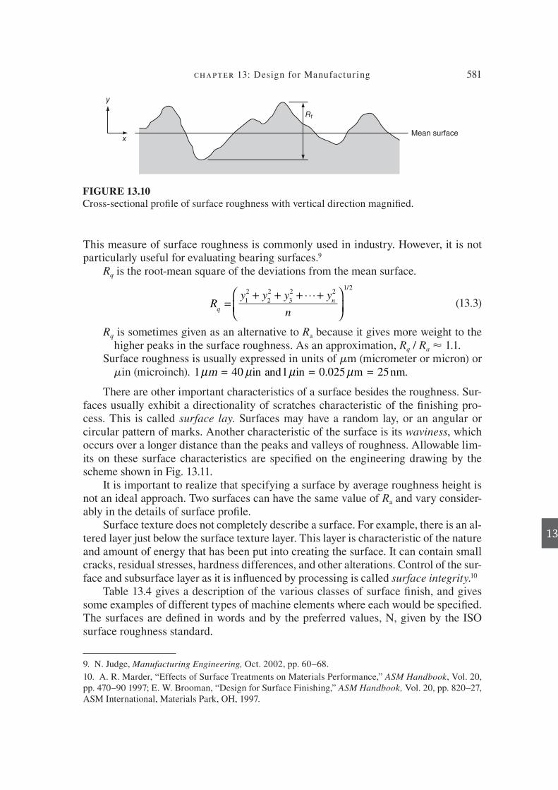
chapter 13: Design for Manufactur ing 581
13
9. N . Judge , Manufacturing Engineering, Oct. 2002 , pp. 60–68.
This measure of surface roughness is commonly used in industry. However, it is not particularly useful for evaluating bearing surfaces. 9
R q is the root-mean square of the deviations from the mean surface.
Ry y y y
nq
n=+ + + ⋅⋅ ⋅ +
12
22
32 2
1 2/
(13.3)
R q is sometimes given as an alternative to Ra because it gives more weight to the higher peaks in the surface roughness. As an approximation, Rq / Ra < 1.1.
Surface roughness is usually expressed in units of mm (micrometer or micron) or min (microinch) . 1 40µ µ µ µm = in and1 in = 0.025 m = 25nm.
There are other important characteristics of a surface besides the roughness. Sur-faces usually exhibit a directionality of scratches characteristic of the > nishing pro-cess. This is called surface lay . Surfaces may have a random lay, or an angular or circular pattern of marks. Another characteristic of the surface is its waviness , which occurs over a longer distance than the peaks and valleys of roughness. Allowable lim-its on these surface characteristics are speci> ed on the engineering drawing by the scheme shown in Fig. 13.11.
It is important to realize that specifying a surface by average roughness height is not an ideal approach. Two surfaces can have the same value of R a and vary consider-ably in the details of surface pro> le.
Surface texture does not completely describe a surface. For example, there is an al-tered layer just below the surface texture layer. This layer is characteristic of the nature and amount of energy that has been put into creating the surface. It can contain small cracks, residual stresses, hardness differences, and other alterations. Control of the sur-face and subsurface layer as it is inR uenced by processing is called surface integrity . 10
Table 13.4 gives a description of the various classes of surface > nish, and gives some examples of different types of machine elements where each would be speci> ed. The surfaces are de> ned in words and by the preferred values, N, given by the ISO surface roughness standard.
10. A. R . Marder , “Effects of Surface Treatments on Materials Performance,” ASM Handbook , Vol. 20, pp. 470–90 1997 ; E. W . Brooman , “Design for Surface Finishing,” ASM Handbook, Vol. 20, pp. 820–27 , ASM International, Materials Park, OH , 1997 .
y
x
Rt
Mean surface
FIGURE 13.10 Cross-sectional pro> le of surface roughness with vertical direction magni> ed.
die37039_ch13.indd 581 2/25/08 6:59:44 PM

582 engineering design
13
Dimensional Accuracy and Tolerances
Processes differ in their ability to meet close tolerances. Generally, materials with good workability can be held to closer tolerances. Achieving dimensional accuracy depends on both the nature of the material and the process. Solidi> cation processes must allow for the shrinkage that occurs when a molten metal solidi> es. Polymer pro-cesses must allow for the much higher thermal expansion of polymers than metals, and hot working processes for metals must allow for oxidation of the surface.
FIGURE 13.11Symbols used to specify > nish characteristics on an engineering drawing. Roughness given in microinches.
Maximum waviness height
Maximum waviness width
Roughness width cutoff
Maximum roughness width
Symbols for lay
Perpendicular toline representing
Parallel to line
Crossed
Random
Circular
Approximate radial
X
M
C
R
Roughness height (Ra): maximum 63
minimum 16
0.002 - 2
0.030
0.020X
Lay
TABLE 13.4
Typical Values for Surface Roughness
Description N-value R a , Min R a , Mm Typical Application in Design
Very rough N11 1000 25.0 Nonstressed surface; rough cast surface
Rough N10 500 12.5 Noncritical components; machined
Medium N9 250 6.3 Most common surface for components
Average smooth N8 125 3.2 Suitable for mating surfaces without motion
Better than avg. N7 63 1.6 Use for close-> tting sliding surfaces an stressed parts except for shafts and vibra-tion conditions.
Fine N6 32 0.8 Use where stress concentration is high; gears, etc.
Very > ne N5 16 0.4 Use for fatigue-loaded parts; precision shafts
Extremely > ne N4 8 0.2 High-quality bearings; requires honing/ polishing
Super> nish N3 4 0.1 For highest precision parts; requires lapping
die37039_ch13.indd 582 2/25/08 6:59:45 PM

chapter 13: Design for Manufactur ing 583
13
FIGURE 13.12 Approximate values of surface roughness and tolerance on dimensions typically obtained with different manufacturing processes. (J. A. Schey, Introduction to Manufacturing Processes, 3d ed.
McGraw-Hill, 2000)
Each manufacturing process has the capability of producing a part to a certain sur-face > nish and tolerance range without incurring extra cost. Figure 13.12 shows this general relationship. The tolerances apply to a 1-inch dimension and are not necessarily scalable to larger and smaller dimensions for all processes. For economical design, the loosest possible tolerances and coarsest surface > nish that will ful> ll the function of the design should be speci> ed. As Fig. 13.13 shows, processing cost increases nearly expo-nentially as the requirements for tolerances and surface > nish are made more stringent.
13.4.6 Cost to Manufacture
The manufacturing cost of the > nished product is the most important factor in deter-mining the selection of the manufacturing process and the material. 11 We did not pres-ent this topic > rst in this section because you > rst needed a better understanding of the other factors that inR uence process selection. An even more detailed consideration of cost is given in Chapter 16.
11. A. M. K . Esawi and M. F . Ashby , “Cost Estimates to Guide Pre-Selection of Processes,” Materials
and Design , vol. 24, pp. 605–616 , 2003 .
1 2 40.5 8 16 32 63 125 250 500 1000 2000
N10.025
N20.05
N30.1
N40.2
N50.4
N60.8
N71.6
N83.2
N96.3
N1012.5
N1125
N1250
ISO No. m!
in!
0.0001
0.001
0.010
0.100
0.005
0.01
0.1
0.5
1.0
2.0
0.05
Permanent m
old
Powder met.
Plaster
ShellSand c
ast
Zn die
Hot roll,
extru
de, forg
e
Polymers
(any
surface
finish)
Al-die ca
st
Inve
stment c
ast
Cold extrude, r
oll
Cold draw
Precision blank
Drill, p
unch
Finish mill
Shape, pla
ne, rough m
ill
Broach
, ream
ECM–EDM
Finish grind
Finish turn, b
ore
Rough grin
d, turn
Polish, lap, hone
mm
To
lera
nce
ra
ng
e,
in.
Surface roughness Ra
die37039_ch13.indd 583 2/25/08 6:59:45 PM

584 engineering design
13
The cost to manufacture a part is made up of the cost of the material C M , the wages of the persons who make the parts and assemble the product, C L , the capitalized cost of the equipment, C C , the cost of tooling, C T , and a cost of overhead, C OH , that lumps together many necessary costs, like plant maintenance, general engineering, and ac-counting, that cannot be directly associated with each unit of product produced.
The > rst cost component of the unit cost , C U, of a part is the weight of material m times the cost of material C M . This must be adjusted by the fraction of material that ends up as scrap, f , due to the sprues and risers that must be cut from castings and molding, or the chips made in machining, or parts that are rejected for defects of some kind.
CC
1 =−( )
m
f
M
1 (13.4)
Next we have the labor cost to make the part, expressed as labor cost (wages and bene> ts) per unit time. If n is the production rate, the number of parts produced per unit time, the labor cost, is given by
CC
2 = L
n& (13.5)
The tooling (dies, molds, > xtures, etc.) that is directly involved with the making a particular part has a cost C T .
CC
3 =k
n
T (13.6)
FIGURE 13.13InR uence of tolerance on processing costs (schematic).
±0.015
Incre
ase
in
co
st,
%
Castor
forged
Roughmachine
Finishmachine
Grind Hone
±0.010 ±0.003 ±0.001 ±0.0005 ±0.00025 Tolerance, in.±0.030
100
200
300
400
0
die37039_ch13.indd 584 2/25/08 6:59:46 PM
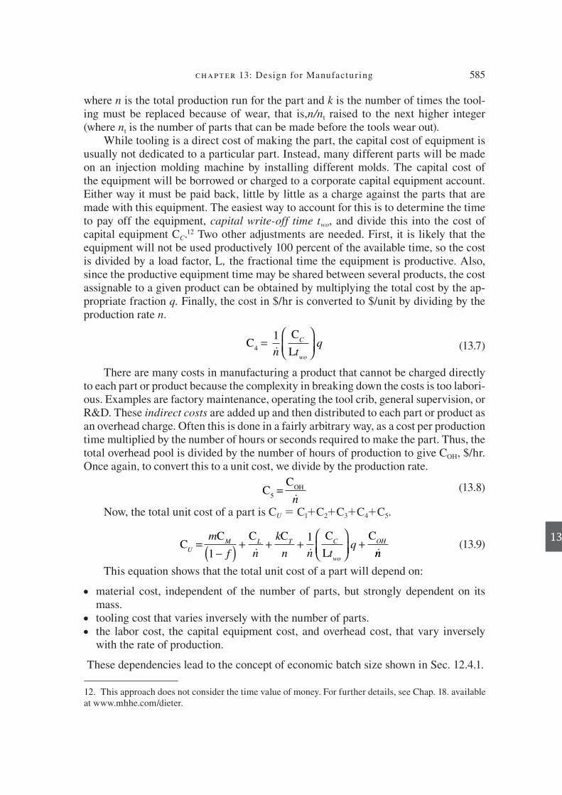
chapter 13: Design for Manufactur ing 585
13
12 . This approach does not consider the time value of money. For further details, see Chap. 18. available at www.mhhe.com/dieter.
where n is the total production run for the part and k is the number of times the tool-ing must be replaced because of wear, that is, n/n t raised to the next higher integer (where n t is the number of parts that can be made before the tools wear out).
While tooling is a direct cost of making the part, the capital cost of equipment is usually not dedicated to a particular part. Instead, many different parts will be made on an injection molding machine by installing different molds. The capital cost of the equipment will be borrowed or charged to a corporate capital equipment account. Either way it must be paid back, little by little as a charge against the parts that are made with this equipment. The easiest way to account for this is to determine the time to pay off the equipment, capital write-off time two , and divide this into the cost of capital equipment C C . 12 Two other adjustments are needed. First, it is likely that the equipment will not be used productively 100 percent of the available time, so the cost is divided by a load factor, L, the fractional time the equipment is productive. Also, since the productive equipment time may be shared between several products, the cost assignable to a given product can be obtained by multiplying the total cost by the ap-propriate fraction q. Finally, the cost in $/hr is converted to $/unit by dividing by the production rate n .
CC
L4 =
1&n t
qC
wo
(13.7)
There are many costs in manufacturing a product that cannot be charged directly to each part or product because the complexity in breaking down the costs is too labori-ous. Examples are factory maintenance, operating the tool crib, general supervision, or R&D. These indirect costs are added up and then distributed to each part or product as an overhead charge. Often this is done in a fairly arbitrary way, as a cost per production time multiplied by the number of hours or seconds required to make the part. Thus, the total overhead pool is divided by the number of hours of production to give C OH , $/hr. Once again, to convert this to a unit cost, we divide by the production rate.
CC
5OH=&n
(13.8)
Now, the total unit cost of a part is C U 5 C 1 1C 2 1C 3 1C 4 1C 5 .
CC C C C
L
CU
M L T C
wo
OHm
f n
k
n n tq=
−( ) + + +
+
1
1& & &nn
(13.9)
This equation shows that the total unit cost of a part will depend on:
material cost, independent of the number of parts, but strongly dependent on its mass.
tooling cost that varies inversely with the number of parts. the labor cost, the capital equipment cost, and overhead cost, that vary inversely with the rate of production.
These dependencies lead to the concept of economic batch size shown in Sec. 12.4.1.
●
●
●
die37039_ch13.indd 585 2/25/08 6:59:46 PM

586 engineering design
13
13.4.7 Availability, Lead Time, and Delivery
Next to cost, a critical business factor in selecting a manufacturing process is the avail-ability of the production equipment, the lead time to make tooling, and the reliability of the expected delivery date for parts made by outside suppliers. Large structural parts, such as rotors for electrical generators, or the main structural forgings for mili-tary aircraft, can be made in only a few factories in the world because of equipment requirements. Careful scheduling with the design cycle may be needed to mesh with the production schedule. Complex forging dies and plastic injection molding dies can have lead times of a year. These kinds of issues clearly affect the choice of the manu-facturing process and demand attention during the embodiment design phase.
13.4.8 Further Information for Process Selection
The book by Schey 13 and the handbook chapter by the same author 14 are particularly helpful in the way they compare a wide spectrum of manufacturing processes. A com-parison of manufacturing processes is given in Table 13.5. This is based on a series of data cards published by the Open University. 15
This table is useful in two ways. First, it gives a quick way to screen for some broad process characteristics.
Shape—the nature of the shapes that can be produced by the process Cycle time—time for a machine cycle to produce one part (1/ n
. ) Flexibility—time to change tooling to make a different part Material utilization—percent of input material that does not end up in > nished part
Quality—level of freedom from defects and ability to hold dimensions to drawing Equipment/tooling costs—level of equipment charges and tooling costs.
The rating scale for ranking processes according to these factors is in Table 13.6. (An-other rating system using a more detailed listing of process characteristics is given by Schey. 16 )
A second useful feature of Table 13.5 is the references to the extensive series of ASM Handbooks (AHB) and Engineered Materials Handbooks (EMH), which give many practical details on the processes.
The Manufacturing Process Information Maps (PRIMA) give much informa-tion that is useful for an initial selection of process. 17 The PRIMA selection matrix
●
●
●
●
●
●
14. J. A. Schey, “Manufacturing Processes and Their Selection,” ASM Handbook, Vol. 20, pp. 687–704, ASM International, Materials Park, OH, 1997.
17. K. G . Swift and J. D . Booker , Process Selection, 2d ed., Butterworth-Heinemann, Oxford, UK , 2003 .
16. J. A . Schey , “Manufacturing Processes and Their Selection,” ASM Handbook, Vol. 20, pp. 687–704 , ASM International, Materials Park, OH , 1997 .
13. J. A. Schey, Introduction to Manufacturing Processes, 3d ed., McGraw-Hill, New York, 2000.
15. Data cards to accompany L. Edwards and M. Endean, eds., Manufacturing with Materials, Butter-worth, Boston, 1990.
die37039_ch13.indd 586 2/25/08 6:59:46 PM

chapter 13: Design for Manufactur ing 587
13
(Fig. 13.9) gives a set of 5 to 10 possible processes for different combinations of mate-rial and quantity of parts. Each PRIMA then gives the following information, which is a good summary of the information needed to make an intelligent decision on the manufacturing process:
Process description Materials: materials typically used with the process Process variations: common variants of the basic process Economic factors: cycle time, minimum production quantity, material utilization, tooling costs, labor costs, lead times, energy costs, equipment costs
Typical applications: examples of parts commonly made with this process Design aspects: general information on shape complexity, size range, minimum thickness, draft angles, undercuts, and limitations on other features
Quality issues: describes defects to watch out for, expected range of surface > n-ish, and process capability charts showing dimensional tolerances as a function of dimension
The book Process Selection is an excellent resource for process selection if the Cam-bridge Selection software is not available.
E X A M P L E 1 3 . 2 The selection of materials for an automobile fan, Example 11.3, was done with the as-sumption that the manufacturing costs for each material would be approximately equal since they were either casting or molding processes. The top-ranked materials were (1) an aluminum casting alloy, (2) a magnesium casting alloy, and (3) nylon 6/6 with 30 percent chopped glass > ber to increase the fracture toughness of the material. Casting or molding were given high consideration since we expect to be able to manufacture the component with the fan blades integrally attached to the fan hub.
Now we need to think more broadly about possible processes for making 500,000 parts per year. Figure 13.9 and Table 13.5 are used to perform a preliminary screening for potential processes before making a > nal decision based on costs calculated from Eq. (13.9). Table 13.7 shows the processes suggested in Fig. 13.9 for an aluminum alloy, a magnesium alloy, and the thermoplastic nylon 6/6.
In interpreting Table 13.7, the > rst consideration was whether Fig. 13.9 indicated that the process was suitable for one of the materials. The matrix of possible processes versus materials shows the greatest number of potential processes for an aluminum alloy, and the fewest for nylon 6/6. The > rst round of screening is made on the basis of the predominant shapes produced by each process. Thus, blow molding was eliminated because it pro-duces thin, hollow shapes, extrusion and drawing because they produce straight shapes with high length-to-diameter ratios and because the blades must have a slight degree of twist. Sheet metal processes were eliminated because they create only 2-D shapes. Ma-chining was declared too costly by management edict. The preliminary screening left the following processes for further consideration:
●
●
●
●
●
●
●
Aluminum alloy Magnesium alloy Nylon 6/6
Shell molding Gravity die casting Injection moldingGravity die casting Pressure die casting
Pressure die casting Closed die forging
Squeeze casting Squecze casting
Closed die forging
die37039_ch13.indd 587 2/25/08 6:59:47 PM

588 engineering design
13
Process ShapeCycle Time Flexibility
Material Utilization Quality
Equipment Tooling Costs
Handbook Reference
Casting
Sand casting 3-D 2 5 2 2 1 AHB, vol. 15
Evaporative foam 3-D 1 5 2 2 4 AHB, vol. 15, p. 230
Investment casting 3-D 2 4 4 4 3 AHB, vol. 15, p. 253
Permanent mold casting
3-D 4 2 2 3 2 AHB, vol. 15, p. 275
Pressure die casting 3-D solid 5 1 4 2 1 AHB, vol. 15, p. 285
Squeeze casting 3-D 3 1 5 4 1 AHB, vol. 15, p. 323
Centrifugal casting
3-D hollow 2 3 5 3 3 AHB, vol. 15, p. 296
Injection molding 3-D 4 1 4 3 1 EMH, vol. 2, p. 308
Reaction injection molding (RIM)
3-D 3 2 4 2 2 EMH, vol. 2, p. 344
Compression molding
3-D 3 4 4 2 3 EMH, vol. 2, p. 324
Rotational molding
3-D hollow 2 4 5 2 4 EMH, vol. 2, p. 360
Monomer casting contact molding
3-D 1 4 4 2 4 EMH, vol. 2, p. 338
Forming
Forging, open die 3-D solid 2 4 3 2 2 AHB, vol. 14A, p. 99
Forging, hot closed die
3-D solid 4 1 3 3 2 AHB, vol. 14A, p. 111, 193
Sheet metal forming
3-D 3 1 3 4 1 AHB, vol. 14B, p. 293
Rolling 2-D 5 3 4 3 2 AHB, vol. 14A, p. 459
Extrusion 2-D 5 3 4 3 2 AHB, vol. 14A, p. 421
Superplastic forming
3-D 1 1 5 4 1 AHB, vol. 14B, p. 350
Thermoforming 3-D 3 2 3 2 3 EMH, vol. 2, p. 399
Blow molding 3-D hollow 4 2 4 4 2 EMH, vol. 2, p. 352Pressing and
sintering3-D solid 2 2 5 2 2 AHB, vol. 7, p. 326
Isostatic pressing 3-D 1 3 5 2 1 AHB, vol. 7, p. 605
Slip casting 3-D 1 5 5 2 4 EMH, vol. 14, p. 153
Machining
Single-point cutting
3-D 2 5 1 5 5 AHB, vol. 16
Multiple-point cutting
3-D 3 5 1 5 4 AHB, vol. 16
Table 13.5 Rating of Characteristics of Common Manufacturing Processes
die37039_ch13.indd 588 2/25/08 6:59:47 PM

chapter 13: Design for Manufactur ing 589
13
Grinding 3-D 2 5 1 5 4 AHB, vol. 16, p. 421
Electrical discharge machining
3-D 1 4 1 5 1 AHB, vol. 16, p. 557
Joining
Fusion welding All 2 5 5 2 4 AHB, vol. 6, p. 175
Brazing/soldering All 2 5 5 3 4 AHB, vol. 6, p. 328, 349
Adhesive bonding All 2 5 5 3 5 EMH, vol. 3
Fasteners 3-D 4 5 4 4 5 . . .
Surface treatment
Shot peening All 2 5 5 4 5 AHB, vol. 5, p. 126
Surface hardening All 2 4 5 4 4 AHB, vol. 5, p. 257
CVD/PVD All 1 5 5 4 3 AHB, vol. 5, p. 510
Rating scheme: 1, poorest; 5, best. From ASM Handbook, Vol. 20, p. 299, ASM International. Used with permission.
Table 13.5 (continued)
TABLE 13.6
Rating Scale for Ranking Manufacturing Processes
Rating Cycle time FlexibilityMaterial Utilization Quality
Equipment Tooling Costs
1 .15 min Changeover very dif> cult
Waste .100% of > nished part
Poor quality High machine and tool-ing costs
2 5 to 15 min Slow changeover Waste 50 t0 100% Average quality Tooling and machines costly
3 1 to 5 min Avg, changeover and setup time
Waste 10 to 50% Average to good quality
Tooling and machines relatively inexpensive
4 20 s to 1 min
Fast changeover Waste , 10% > nished part
Good to excellent
Tooling costs low
5 ,20 s No setup time No appreciable waste
Excellent quality
Equip. and tool very low
Rating scale; 1–poorest; 5–best
It is clear that injection molding is the only feasible process for the thermoplastic ny-lon 6/6. The available processes for aluminum or magnesium alloy come down to several casting processes and closed die forging. These remaining processes are compared using the selection criteria given in Table 13.5 and enumerated at the beginning of Sec.13.3.7. Investment casting is added as an additional process because it is known to make high-quality castings. Data for shell molding is not listed in Table 13.5, but its entry in
Process ShapeCycle Time Flexibility
Material Utilization Quality
Equipment Tooling Costs
Handbook Reference
die37039_ch13.indd 589 2/25/08 6:59:48 PM

590 engineering design
13
TABLE 13.7
Initial Screening of Candidate Processes
Aluminum Alloy Magnesium Alloy Nylon 6/6Reason for Elimination
Possible ProcessYes or
No? Reject?Yes or
No? Reject?Yes or
No? Reject?
1.2 Shell molding Y N N
1.3 Gravity die casting Y Y N
1.4 Pressure die casting Y Y N
1.9 Squeeze casting Y Y N
2.1 Injection molding N N Y
2.6 Blow molding N N Y RUsed for 3-D hollow
shapes
2.9 Plastic extrusion N N Y R Need to twist the blades
3.1 Closed die forging Y Y N
3.2 Rolling Y N N2-D process for making
sheet
3.3 Drawing Y R Y R N Makes shapes with
high L/D
3.4 Cold forming Y R Y R NUsed for hollow 3-D
shapes
3.5 Cold heading Y R N R N Used for making bolts
3.8 Sheet shearing Y R Y R N A 2-D forming process
3.12 Metal extrusion Y R Y R N Need to twist the blades
4A Automatic machining
Y R Y R NMachining is ruled out by edict.
Table 13.8 was constructed from data given in Process Selection. The gravity die casting process is most commonly found under the name of permanent mold casting, and the data for permanent mold casting from Table 13.5 was used in Table 13.8. The rating for each criterion is totaled for each process, as seen in Table 13.8.
The results of this process ranking are not very discriminating. All casting processes rank 13 or 14, except investment casting. The ranking for hot forging is slightly lower at 12. Moreover, designing a forging die to produce a part with 12 blades integrally attached to the fan hub is more dif> cult than designing a casting mold for the same shape. For this application there appears to be no advantage of forging over casting, and since the com-pany does not have in-house forging capability, the forged fan component would have to be provided by an outside supplier. The next step in deciding on the manufacturing process is to compare the esti-
mated cost to manufacture a part using Eq. (13.9). The following processes will be compared: injection molding for nylon 6/6, and low-pressure permanent mold casting, investment casting, and squeeze casting for metal alloys. Squeeze casting is included because it has the potential to produce low-porosity, > ne detail castings when com-pared to shell molding and pressure die casting.
die37039_ch13.indd 590 2/25/08 6:59:48 PM
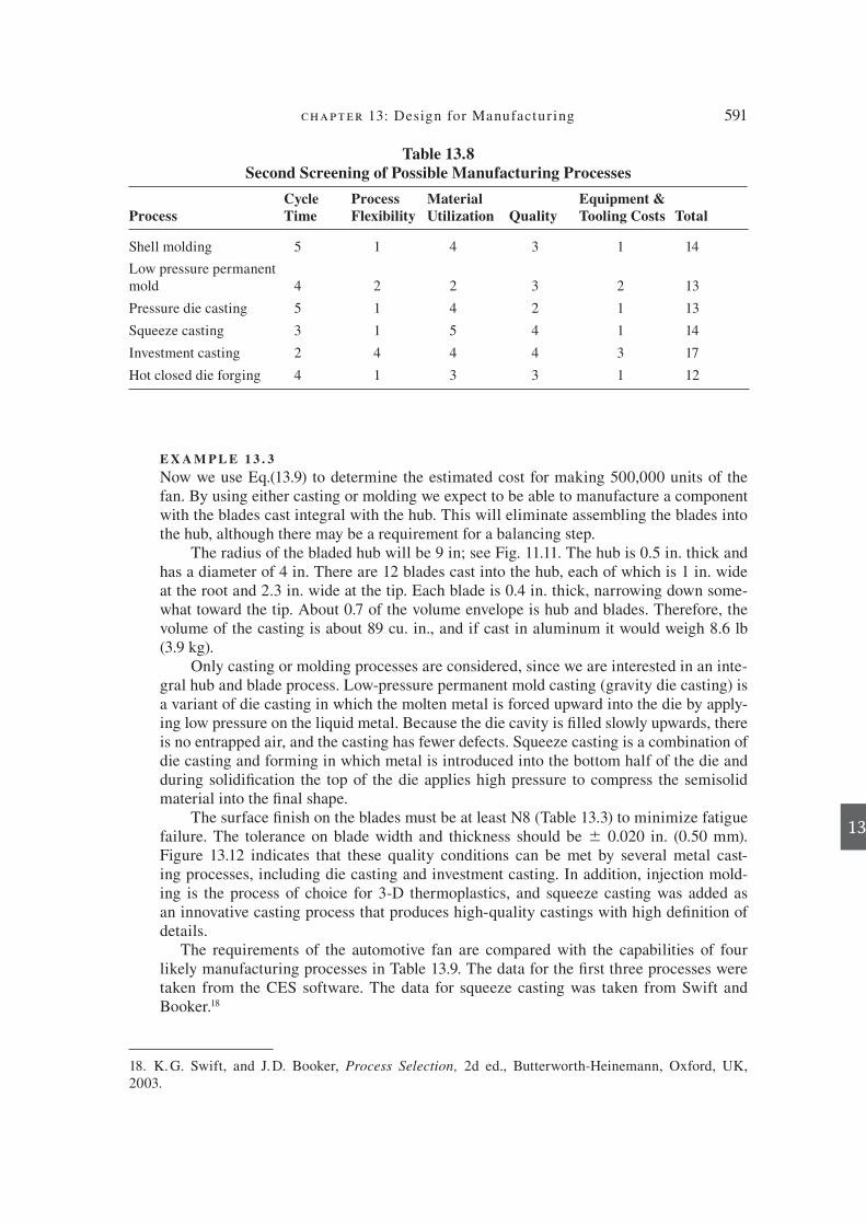
chapter 13: Design for Manufactur ing 591
13
E X A M P L E 1 3 . 3
Now we use Eq.(13.9) to determine the estimated cost for making 500,000 units of the fan. By using either casting or molding we expect to be able to manufacture a component with the blades cast integral with the hub. This will eliminate assembling the blades into the hub, although there may be a requirement for a balancing step.
The radius of the bladed hub will be 9 in; see Fig. 11.11. The hub is 0.5 in. thick and has a diameter of 4 in. There are 12 blades cast into the hub, each of which is 1 in. wide at the root and 2.3 in. wide at the tip. Each blade is 0.4 in. thick, narrowing down some-what toward the tip. About 0.7 of the volume envelope is hub and blades. Therefore, the volume of the casting is about 89 cu. in., and if cast in aluminum it would weigh 8.6 lb (3.9 kg).
Only casting or molding processes are considered, since we are interested in an inte-gral hub and blade process. Low-pressure permanent mold casting (gravity die casting) is a variant of die casting in which the molten metal is forced upward into the die by apply-ing low pressure on the liquid metal. Because the die cavity is > lled slowly upwards, there is no entrapped air, and the casting has fewer defects. Squeeze casting is a combination of die casting and forming in which metal is introduced into the bottom half of the die and during solidi> cation the top of the die applies high pressure to compress the semisolid material into the > nal shape.
The surface > nish on the blades must be at least N8 (Table 13.3) to minimize fatigue failure. The tolerance on blade width and thickness should be " 0.020 in. (0.50 mm). Figure 13.12 indicates that these quality conditions can be met by several metal cast-ing processes, including die casting and investment casting. In addition, injection mold-ing is the process of choice for 3-D thermoplastics, and squeeze casting was added as an innovative casting process that produces high-quality castings with high de> nition of details.
The requirements of the automotive fan are compared with the capabilities of four likely manufacturing processes in Table 13.9. The data for the > rst three processes were taken from the CES software. The data for squeeze casting was taken from Swift and Booker. 18
Table 13.8 Second Screening of Possible Manufacturing Processes
ProcessCycle Time
Process Flexibility
Material Utilization Quality
Equipment & Tooling Costs Total
Shell molding 5 1 4 3 1 14
Low pressure permanent mold 4 2 2 3 2 13
Pressure die casting 5 1 4 2 1 13
Squeeze casting 3 1 5 4 1 14
Investment casting 2 4 4 4 3 17
Hot closed die forging 4 1 3 3 1 12
18. K. G . Swift , and J. D . Booker , Process Selection, 2d ed., Butterworth-Heinemann, Oxford, UK , 2003 .
die37039_ch13.indd 591 2/25/08 6:59:49 PM

592 engineering design
13
Each of the candidate processes is capable of producing symmetrical 3-D shapes. The screening parameter examined > rst was the economic batch size. Since it is expected that 500,000 units will be produced per year, investment casting was eliminated as a pos-sibility because the economic batch size is less than 1000 units. Several of the other pro-cesses have borderline issues with respect to process capability, but they do not disqualify them from further analysis. For example, it may not be possible to obtain the maximum thickness of 13 mm with injection molding of nylon. This de> ciency could be overcome by a different design of the hub using thinner sections and stiffening ribs; see Sec. 12.6.2 There is also a possibility that low-pressure permanent mold casting may not be able to achieve the required tolerance on critical dimensions. Experiments with process variables such as melt temperature and cooling rate will determine whether this proves to be a problem.
Now that we have narrowed the selection of a manufacturing process down to three alternatives, the > nal selection is based on the estimate of the cost to make one unit of the integral hub–blade fan using the cost model described in Sec. 13.4.6.
Calculations show that two machines operating three shifts for 50 weeks per year will be required to produce 500,000 units per year. This is reR ected in the tooling and capital costs. Labor cost is based on one operator per machine. For the permanent mold casting and squeeze casting processes the material is A357 aluminum alloy. For injec-tion molding the material used is nylon 6/6 reinforced with 30 percent chopped glass > bers.
It is clear from Table 13.10 that the cost of the material is the major cost category. It varies from 54% to 69% of total unit cost for the three processes studied. The production rate is also an important process parameter. It accounts for the higher cost of squeeze casting over permanent mold casting in the categories of labor cost and overhead. Process engineering studies using some of the TQM methods discussed in Chap. 4 might be able to increase the rate of production. However, there are physical limits to increasing this rate very greatly since all three processes are limited by the heat transfer rate that de-termines the time required to solidify the part suf> ciently that it can be ejected from the mold.
TABLE 13.9
Comparison of Characteristics of Each Process with Requirements of the Fan
Process RequirementsFan
Design
Low-Pressure Permanent
Mold CastingInvestment
CastingInjection Molding
Squeeze Casting
Size range, max mass (kg) (Fig. 13.7)
3.9 80 30 4.5
Section thickness, max (mm) (Fig. 13.8)
13 120 8 200
Section thickness, min (mm) . . . (Fig. 13.8)
7.5 3 0.6 6
Tolerance ("mm) 0.50 0.5 0.1 0.3
Surface roughness ( mm) Ra 3.2 4 0.2 1.6
Economic batch size, units (Fig. 13.5)
5 3 105 .103 ,103 .105 .104
die37039_ch13.indd 592 2/25/08 6:59:49 PM
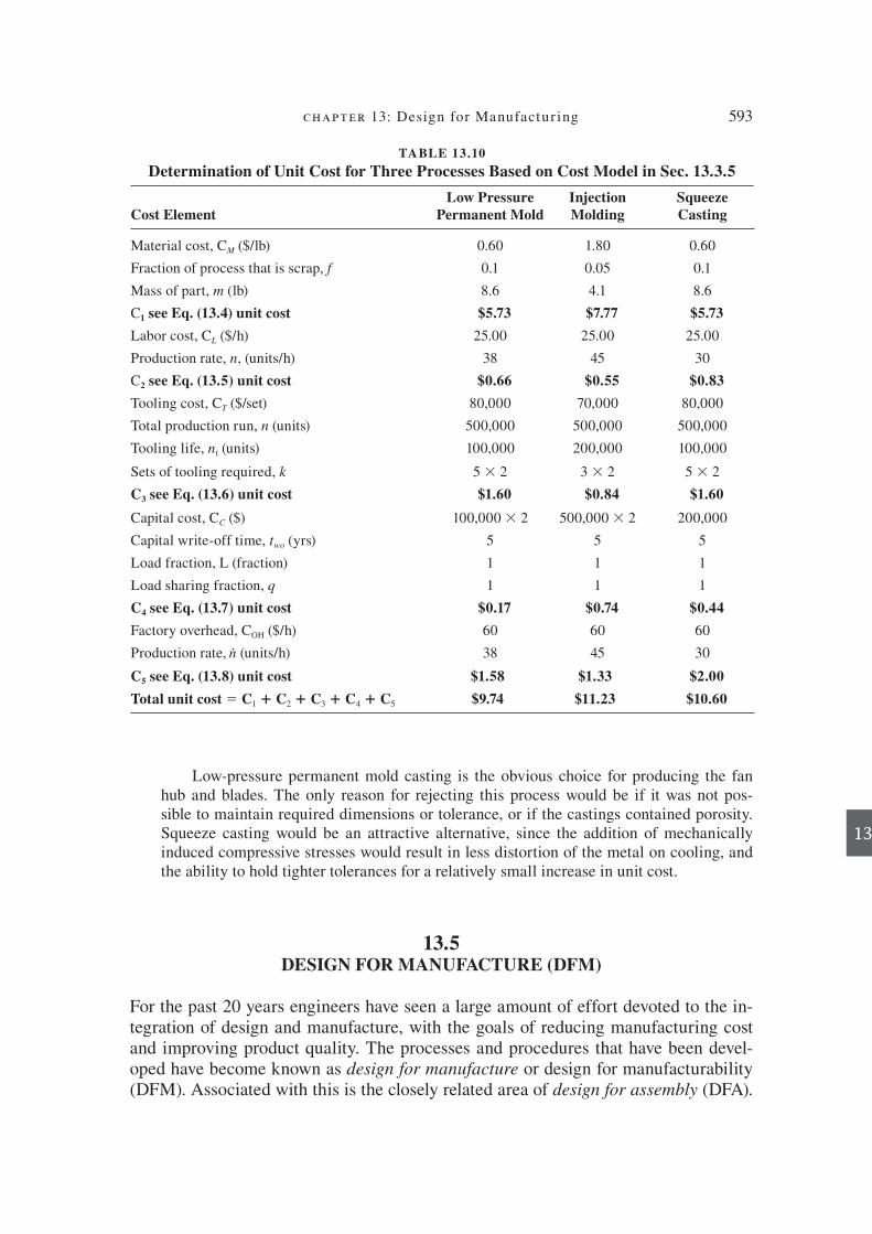
chapter 13: Design for Manufactur ing 593
13
Low-pressure permanent mold casting is the obvious choice for producing the fan hub and blades. The only reason for rejecting this process would be if it was not pos-sible to maintain required dimensions or tolerance, or if the castings contained porosity. Squeeze casting would be an attractive alternative, since the addition of mechanically induced compressive stresses would result in less distortion of the metal on cooling, and the ability to hold tighter tolerances for a relatively small increase in unit cost.
13.5 DESIGN FOR MANUFACTURE (DFM)
For the past 20 years engineers have seen a large amount of effort devoted to the in-tegration of design and manufacture, with the goals of reducing manufacturing cost and improving product quality. The processes and procedures that have been devel-oped have become known as design for manufacture or design for manufacturability (DFM). Associated with this is the closely related area of design for assembly (DFA).
TABLE 13.10
Determination of Unit Cost for Three Processes Based on Cost Model in Sec. 13.3.5
Cost ElementLow Pressure
Permanent MoldInjection Molding
Squeeze Casting
Material cost, CM ($/lb) 0.60 1.80 0.60
Fraction of process that is scrap, f 0.1 0.05 0.1
Mass of part, m (lb) 8.6 4.1 8.6
C1 see Eq. (13.4) unit cost $5.73 $7.77 $5.73
Labor cost, CL ($/h) 25.00 25.00 25.00
Production rate, n, (units/h) 38 45 30
C2 see Eq. (13.5) unit cost $0.66 $0.55 $0.83
Tooling cost, CT ($/set) 80,000 70,000 80,000
Total production run, n (units) 500,000 500,000 500,000
Tooling life, nt (units) 100,000 200,000 100,000
Sets of tooling required, k 5 3 2 3 3 2 5 3 2
C3 see Eq. (13.6) unit cost $1.60 $0.84 $1.60
Capital cost, CC ($) 100,000 3 2 500,000 3 2 200,000
Capital write-off time, two (yrs) 5 5 5
Load fraction, L (fraction) 1 1 1
Load sharing fraction, q 1 1 1
C4 see Eq. (13.7) unit cost $0.17 $0.74 $0.44
Factory overhead, COH ($/h) 60 60 60
Production rate, . n (units/h) 38 45 30
C5 see Eq. (13.8) unit cost $1.58 $1.33 $2.00
Total unit cost 5 C1 C2 C3 C4 C5 $9.74 $11.23 $10.60
die37039_ch13.indd 593 2/25/08 6:59:49 PM

594 engineering design
13
The > eld is often simply described by the abbreviation DFM/DFA or DFMA. DFMA methods should be applied during the embodiment stage of design.
Design for manufacture represents an awareness of the importance of design as the time for thoughtful consideration of all steps of production. To achieve the goals of DFM requires a concurrent engineering team approach (Sec. 2.4.4) in which appro-priate representatives from manufacturing, including outside suppliers, are members of the design team from the start.
13.5.1 DFM Guidelines
DFM guidelines are statements of good design practice that have been empirically derived from years of experience. 19 Using these guidelines helps narrow the range of possibilities so that the mass of detail that must be considered is within the capability of the designer.
Minimize total number of parts: Eliminating parts results in great savings. A part that is eliminated costs nothing to make, assemble, move, store, clean, in-spect, rework, or service. A part is a good candidate for elimination if there is no need for relative motion, no need for subsequent adjustment between parts, and no need for materials to be different. However, part reduction should not go so far that it adds cost because the remaining parts become too heavy or complex.
The best way to eliminate parts is to make minimum part count a requirement of the design at the conceptual stage of design. Combining two or more parts into an integral design architecture is another approach. Plastic parts are particularly well suited for integral design. 20 Fasteners are often prime targets for part reduc-tion. Another advantage of making parts from plastics is the opportunity to use snap-> ts instead of screws, Fig. 13.14a. 21 Standardize components: Costs are minimized and quality is enhanced when standard commercially available components are used in design. The bene> ts also occur when a company standardizes on a minimum number of part designs (sizes, materials, processes) that are produced internally in its factories. The life and reli-ability of standard components may have already been established, so cost reduc-tion comes through quantity discounts, elimination of design effort, avoidance of equipment and tooling costs, and better inventory control. Use common parts across product lines: It is good business sense to use parts in more than one product. Specify the same materials, parts, and subassem-blies in each product as much as possible. This provides economies of scale that drive down unit cost and simplify operator training and process control. Product
1.
2.
3.
21. P. R . Bonnenberger , The First Snap-Fit Handbook, 2d ed., Hanser Gardener Publications Cincinnati, OH , 2005 .
20. W . Chow , Cost Reduction in Product Design, chap. 5, Van Nostrand Reinhold, New York , 1978 .
19. H. W. Stoll, Appl. Mech. Rev, Vol. 39, No. 9, pp. 1356–64, 1986; J.R. Bralla, Design for Manufactur-
ability Handbook, 2d ed., McGraw-Hill, New York, 1999; D. M. Anderson, Design for Manufacturabil-
ity,, 2d ed., CIM Press, Cambria, CA, 2001.
die37039_ch13.indd 594 2/25/08 6:59:50 PM

chapter 13: Design for Manufactur ing 595
13
data management (PDM) systems can be used to facilitate retrieval of similar designs. Standardize design features. Standardizing on design features like drilled hole sizes, screw thread types, and bend radii minimizes the number of tools that must be maintained in the tool room. This reduces manufacturing cost. Aim to keep designs functional and simple: Achieving functionality is para-mount, but don’t specify more performance than is needed. It is not good engi-neering to specify a heat-treated alloy steel when a plain carbon steel will achieve the performance with a little bit more careful analysis. When adding features to the design of a component, have a > rm reason for the need. The product with the fewest parts, the least intricate shapes, the fewer precision adjustments, and the lowest number of manufacturing steps will be the least costly to manufac-ture. Also, the simplest design will usually be the most reliable and the easiest to maintain. Design parts to be multifunctional: A good way to minimize part count is to design such that parts can ful> ll more than one function, leading to integral architecture. For example, a part might serve as both a structural member and a spring, Fig. 13.14 b . The part might be designed to provide a guiding, aligning, or self-> xturing feature in assembly. This rule can cancel out guideline 5 and break guideline 7 if it is carried too far.
4.
5.
6.
FIGURE 13.14Some examples of applying DFM. (a) This product utilizes snap-> t principles to attach the cover, eliminating the need for screw fasteners. Since the cover is molded from plastic mate-rial and because of the taper of the snap-> t elements, it also illustrates compliance. (b) This illustrates a multifunctional part. By incorporating a spring function in the lever, the need for a separate coil spring is eliminated.
Plastic cover
Lever
Spring featureSpring
(b)
(a)
die37039_ch13.indd 595 2/25/08 6:59:50 PM
596 engineering design
13
Design parts for ease of fabrication: As discussed in Chap. 11, the least costly material that satis> es the functional requirements should be chosen. It is often the case that materials with higher strength have poorer workability or fabricability. Thus, one pays more for a higher-strength material, and it also costs more to pro-cess it into the required shape. Since machining to shape tends to be costly, manu-facturing processes that produce the part to near net shape are preferred whenever possible so as to eliminate or minimize machining.
It is important to be able to visualize the steps that a machine operator will use to make a part so that you can minimize the manufacturing operations needed to make the part. For example, clamping a part before machining is a time-consuming activity, so design to minimize the number of times the operator will be required to reorient the part in the machine to complete the machining task. Reclamping also is a major source of geometric errors. Consider the needs for the use of > xtures and provide large solid mounting surfaces and parallel clamping surfaces.
Rough evaluations for how easily speci> c materials can be processed by dif-ferent manufacturing methods are given in Fig. 13.17. Guidelines for speci> c pro-cesses are given in Secs. 13.11 to 13.19. Avoid excessively tight tolerances: Tolerances must be set with great care. Specifying tolerances that are tighter than needed results in increased cost; recall Fig. 13.13. These come about from the need for secondary > nishing operations like grinding, honing, and lapping, from the cost of building extra precision into the tooling, from longer operating cycles because the operator is taking > ner cuts, and from the need for more skilled workers. Before selecting a manufacturing process, be sure that it is capable of producing the needed tolerance and surface > nish.
As a designer, it is important to maintain your credibility with manufactur-ing concerning tolerances. If in doubt that a tolerance can be achieved in produc-tion, always communicate with manufacturing experts. Never give a verbal agree-ment to manufacturing that they can loosen a tolerance without documentation and making the change on the part drawing. Also, be careful about how the statement for blanket tolerances on the drawing is worded and might be misinterpreted by manufacturing. Minimize secondary and d nishing operations: Minimize secondary operations such as heat treatment, machining, and joining and avoid > nishing operations such as deburring, painting, plating, and polishing. Use only when there is a functional reason for doing so. Machine a surface only when the functionality requires it or if it is needed for aesthetic purposes. Utilize the special characteristics of processes: Be alert to the special design features that many processes provide. For example, molded polymers can be pro-vided with “built-in” color, as opposed to metals that need to be painted or plated. Aluminum extrusions can be made in intricate cross sections that can then be cut to short lengths to provide parts. Powder-metal parts can be made with controlled porosity that provides self-lubricating bearings.
These rules are becoming the norm in every engineering design course and in engineering practice.
7.
8.
9.
10.
die37039_ch13.indd 596 2/25/08 6:59:51 PM

chapter 13: Design for Manufactur ing 597
13
13.5.2 Specid c Design Rules
A number of DFM rules for design, more speci> c than the preceding guidelines, have been developed. 22
Space holes in machined, cast, molded, or stamped parts so they can be made in one operation without tooling weakness. This means that there is a limit on how close holes may be spaced due to strength in the thin section between holes. Avoid generalized statements on drawings, like “polish this surface” or “toolmarks not permitted,” which are dif> cult for manufacturing personnel to interpret. Notes on engineering drawings must be speci> c and unambiguous. Dimensions should be made from speci> c surfaces or points on the part, not from points in space. This greatly facilitates the making of gages and > xtures. The use of GD&T methods makes this point moot. Dimensions should all be from a single datum surface rather than from a variety of points to avoid overlap of tolerances. The design should aim for minimum weight consistent with strength and stiffness requirements. While material costs are minimized by this criterion, there also will usually be a reduction in labor and tooling costs. Whenever possible, design to use general-purpose tooling rather than special dies, form cutters, and similar tools. An exception is high-volume production where special tooling may be more cost-effective. Use generous > llets and radii on castings and on molded, formed, and machined parts. Parts should be designed so that as many operations as possible can be performed without requiring repositioning. This promotes accuracy and minimizes handling.
It is valuable to have manufacturing engineers and specialists involved in design deci-sion making so that these guidelines and others they bring can inform the process.
13.6 DESIGN FOR ASSEMBLY (DFA)
Once parts are manufactured, they need to be assembled into subassemblies and products. The assembly process consists of two operations, handling , which involves grasping, orienting, and positioning, followed by insertion and fastening . There are three types of assembly, classi> ed by the level of automation. In manual assembly a human operator at a workstation reaches and grasps a part from a tray, and then moves, orients, and pre-positions the part for insertion. The operator then places the parts together and fastens them, often with a power tool. In automatic assembly, han-dling is accomplished with a parts feeder, like a vibratory bowl, that feeds the cor-
1.
2.
3.
4.
5.
6.
7.
8.
22. J. R . Bralla , Design for Manufacturability Handbook, 2d ed., McGraw-Hill, New York , 1999 .
die37039_ch13.indd 597 2/25/08 6:59:51 PM

598 engineering design
13
rectly oriented parts for insertion to an automatic workhead, which in turn inserts the part. 23 In robotic assembly, the handling and insertion of the part is done by a robot arm under computer control.
The cost of assembly is determined by the number of parts in the assembly and the ease with which the parts can be handled, inserted, and fastened. Design can have a strong inR uence in both areas. Reduction in the number of parts can be achieved by elimination of parts (e.g., replacing screws and washers with snap or press > ts, and by combining several parts into a single component). Ease of handling and insertion is achieved by designing so that the parts cannot become tangled or nested in each other, and by designing with symmetry in mind. Parts that do not require end-to-end orientation prior to insertion, as a screw does, should be used if possible. Parts with complete rotational symmetry around the axis of insertion, like a washer, are best. When using automatic handling it is better to make a part highly asymmetric if it can-not be made symmetrical.
For ease of insertion, a part should be made with chamfers or recesses for ease of alignment, and clearances should be generous to reduce the resistance to assembly. Self-locating features are important, as is providing unobstructed vision and room for hand access. Figure 13.15 illustrates some of these points.
13.6.1 DFA Guidelines
The guidelines for design for assembly can be grouped into three classes: general, handling, and insertion.
General Guidelines
Minimize the total number of parts: A part that is not required by the design is a part that does not need to be assembled. Go through the list of parts in the assembly and identify those parts that are essential for the proper functioning of the product. All others are candidates for elimination. The criteria for an essential
part , also called a theoretical part, are: ● The part must exhibit motion relative to another part that is declared essential. ● There is a fundamental reason that the part be made from a material different
from all other parts. ● It would not be possible to assemble or disassemble the other parts unless this
part is separate, that is it is an essential connection between parts. ● Maintenance of the product may require disassembly and replacement of a
part. ● Parts used only for fastening or connecting other parts are prime candidates for
elimination.
1.
23. G . Boothroyd , Assembly Automation and Product Design, 2d ed., CRC Press, Boca Raton, FL , 2005 ; “Quality Control and Assembly,” Tool and Manufacturing Engineers Handbook , Vol. 4, Society of Manufacturing Engineers, Dearborn, MI 1987 .
die37039_ch13.indd 598 2/25/08 6:59:51 PM

chapter 13: Design for Manufactur ing 599
13
Designs can be evaluated for ef> ciency of assembly with Eq. (13.10), where the time taken to assemble a “theoretical” part is taken as 3 seconds. 24
Designassembly efficiency“theoretical” m
=×3 iinimum number of parts
total assembly timefor aall parts (13.10)
A theoretical part is one that cannot be eliminated from the design because it is needed for functionality. Typical > rst designs have assembly ef> ciencies of 5 to 10 percent, while after DFA analysis it is typically around 20 to 30 percent.
Minimize the assembly surfaces: Simplify the design so that fewer surfaces need to be prepared in assembly, and all work on one surface is completed before mov-ing to the next one.
2.
FIGURE 13.15Some design features that improve assembly.
Difficult to orientate
small chamfer on chip
with mechanical tooling
Non-functional
longitudinal feature
simplifies orientation
Component does not
have a stable orientation
Flats on the sides make
it easy to orientate with
respect to small holes
Straight slot will tangle
Provide guide on
surfaces to aid
component placing
Crank slot will not tangle
Poor Assembly Improved Assembly
24. For small parts such as those found in household and electronic products, the assembly time runs from 2 to 10 seconds. On an automobile assembly line, times of 45 to 60 seconds are more typical.
die37039_ch13.indd 599 2/25/08 6:59:52 PM

600 engineering design
13
Use subassemblies: Subassemblies can provide economies in assembly since there are fewer interfaces in > nal assembly. Subassemblies can also be built and tested elsewhere and brought to the > nal assembly area. When subassemblies are pur-chased they should be delivered fully assembled and tested. Products made from subassemblies are easier to repair by replacing the defective subassembly. Mistake-proof the design and assembly: An important goal in design for as-sembly is to ensure that the assembly process is unambiguous so that the opera-tors cannot make mistakes in assembling the components. Components should be designed so that they can only be assembled one way. The way to orient the part in grasping it should be obvious. It should not be capable of being assembled in the reverse direction. Orientation notches, asymmetrical holes, and stops in assembly > xtures are common ways to mistake-proof the assembly process. For more on mistake-proo> ng, see Sec. 13.8.
Guidelines for Handling
Avoid separate fasteners or minimize fastener costs: Fasteners may amount to only 5 percent of the material cost of a product, but the labor they require for proper handling in assembly can reach 75 percent of the assembly costs. The use of screws in assembly is expensive. Snap > ts should be used whenever possible. When the design permits, use fewer large fasteners rather than several small ones. Costs associated with fasteners can be minimized by standardizing on a few types and sizes of fasteners, fastener tools, and fastener torque settings. When a product is assembled with a single type of screw fastener it is possible to use auto-feed power screwdrivers. Minimize handling in assembly: Parts should be designed to make the required position for insertion or joining easy to achieve. Since the number of positions required in assembly equates to increased equipment expense and greater risk of defects, quality parts should be made as symmetrical as their function will allow. Orientation can be assisted by design features that help to guide and locate parts in the proper position. Parts that are to be handled by robots should have a R at, smooth top surface for vacuum grippers, or an inner hole for spearing, or a cylin-drical outer surface for gripper pickup.
Guidelines for Insertion
Minimize assembly direction: All products should be designed so that they can be assembled from one direction. Rotation of an assembly requires extra time and motion and may require additional transfer stations and > xtures. The best situa-tion in assembly is when parts are added in a top-down manner to create a z-axis stack. Provide unobstructed access for parts and tools: Not only must the part be de-signed to > t in its prescribed location, but there must be an adequate assembly path for the part to be moved to this location. This also includes room for the operator’s arm and tools, which in addition to screwdrivers, could include wrenches or weld-ing torches. If a worker has to go through contortions to perform an assembly op-eration, productivity and possibly product quality will suffer after a few hours of work.
3.
4.
5.
6.
7.
8.
die37039_ch13.indd 600 2/25/08 6:59:52 PM

chapter 13: Design for Manufactur ing 601
13
Maximize compliance in assembly: Excessive assembly force may be required when parts are not identical or perfectly made. Allowance for this should be made in the product design. Designed-in compliance features include the use of generous tapers, chamfers, and radii. If possible, one of the components of the product can be designed as the part to which other parts are added (part base) and as the as-sembly > xture. This may require design features that are not needed for the prod-uct function.
13.7 ROLE OF STANDARDIZATION IN DFMA
In Section 1.7 the important role of codes and standards in engineering design was in-troduced. There the emphasis was on the role of standards in protecting public safety and assisting the designer in performing high-quality work. In this section we extend these ideas about standardization to show the important role that part standardization can play in DFMA.
Part proliferation is an endemic problem in manufacturing unless steps are taken to prevent it from happening. One large automotive manufacturer found that in one model line alone it used 110 different radiators, 1200 types of R oor carpet, and 5000 different fasteners. Reducing the variety of parts that achieve the same function can have many bene> ts to the product development enterprise. Firm numbers on the cost of part proliferation are dif> cult to obtain, but estimates are that about half of manu-facturing overhead costs are related to managing too many part numbers.
13.7.1 Bened ts of Standardization
The bene> ts of standardization occur in four areas: cost reduction, quality improve-ment, production R exibility, and manufacturing responsiveness. 25 The speci> cs of bene> ts in each area are outlined here.
Cost Reduction
Purchasing costs. Standardization of parts and the subsequent reduction in part numbers 26 will result in large savings in procurement costs in outsourcing because parts will be bought in larger quantities. This allows for quantity discounts, R exible delivery schedules, and less work for the purchasing department.
Reduce costs through raw material standardization. Cost for in-house produc-tion of parts can be reduced if raw materials can be standardized to a single size of bar stock, tubing, and sheet metal. Also, metal casting and plastic molding opera-tions can each be limited to a single material. These standardization efforts allow for increased use of automated equipment with a minimum of cost for tool and > xture changing and setup.
9.
●
●
25. D. M. Anderson, Design for Manufacturability, 2d ed., Chap. 5 CIM Press, Cambria, CA, 2001. 26 . A part number is the identi> cation for a part (often a drawing number) and is not to be confused with the number of parts.
die37039_ch13.indd 601 2/25/08 6:59:52 PM

602 engineering design
13
Feature standardization. Part features such as drilled, reamed, or threaded holes and bend radii in sheet metal all require special tools. Unless there is a dedicated machine for each size, the tools need to be changed for different dimensions, with the corresponding setup charge. Designers often specify an arbitrary hole size, when a standard size would do just as well. If the speci> cation of radii in lathe turning or milling is not standardized it can cause a requirement for the shop to maintain a large inventory of cutting tools.
Reduction of inventory and V oor space requirements. The preceding cost reduc-tion tactics assist in decreasing inventory costs either as incoming parts inventory, or the work-in-progress inventory, through fewer machine setups. Standardiza-tion makes building-on-demand more of a possibility, which will greatly decrease > nished goods inventory. Reducing inventory has the advantage of reducing the required factory R oor space. All of these issues, reduction of inventory and R oor space, tooling costs, and purchasing and other administrative costs result in a de-crease in overhead costs.
Quality Improvement
Product quality. Having fewer parts of a given type greatly reduces the chance of using the wrong part in an assembly.
Prequalid cation of parts. The use of standard parts means that there is much greater cumulative experience with using the particular part. This means that stan-dard parts can be prequali> ed for use in a new product without the requirement for extensive testing.
Supplier reduction means improved quality. Standardization of parts means there will be fewer outside suppliers of parts. Those suppliers remaining should be those with a record of producing quality parts. Giving more business to fewer sup-pliers will be an incentive for developing stronger supplier relationships.
Production Flexibility
Material logistics. The R ow of parts within the plant will be easier with fewer parts to order, receive, stock, issue, assemble, test, and reorder.
Reliable delivery of standard low-cost parts. These parts can be restocked di-rectly to points of use in the plant by parts suppliers using long-term purchase agreements, much as food is delivered to a supermarket. This reduces overhead costs for purchasing and materials handling.
Flexible manufacturing. Eliminating setup operations allows products to be made in any batch size. This allows the products to be made to order or to mass custom-
ize the product. This eliminates > nished goods inventory and lets the plant make only the products for which it has an order.
Manufacturing Responsiveness
Parts availability. Fewer part types used in greater volume will mean less chance of running out of parts and delaying production.
Quicker supplier deliveries. Standardization of parts and materials should speed up deliveries. Suppliers will have the standard tools and materials in their inventory.
●
●
●
●
●
●
●
●
●
●
die37039_ch13.indd 602 2/25/08 6:59:53 PM

chapter 13: Design for Manufactur ing 603
13
Financially stronger suppliers. Part suppliers to OEMs have seen their pro> t mar-gins narrow, and many have gone out of business. With larger volume orders and fewer part types to make, they can rationalize their business model, simplify their supply chain management, and reduce overhead costs. This will give them the re-sources to improve the quality and ef> ciency of their operations.
While the bene> ts from standardization seem very compelling, it may not always be the best course of action. For example, the compromises required by standardization may restrict the design and marketing options in undesirable ways. Stoll 27 presents pros and cons about part standardization.
13.7.2 Achieving Part Standardization
Many engineers do not realize that regardless of the cost of a part, there is real cost in ordering, shipping, receiving, inspecting, warehousing, and delivering the part to where it will be used on the assembly line. Thus, it is just as important to be con-cerned with standardization of inexpensive parts like fasteners, washers, and resistors as it is with more intricate molded parts. Young engineers need to be made aware of the importance of part standardization, and, they should understand that they are not free to make arbitrary decisions when sizing parts. Early in their careers they should be made aware of the company standard part list, and if one does not exist they should work with their colleagues to develop one. 28
A common misconception is that the way to achieve a minimum-cost design is to create a minimum-weight design. Certainly this may be true in aircraft and space-craft design where weight is very important, but for most product design this design philosophy should not be followed if it means using nonstandard parts. The most eco-nomical approach is to select the next larger standard size of motor, pump, or angle iron to achieve adequate strength or functionality. Special sizes are justi> ed only in very special situations.
A common reason for the existence of part duplication is that the designer is not aware of the existence of an identical part. Even if she knows of its existence, it may be more dif> cult to > nd the part number and part drawing than it is to create a new part. This issue is discussed in Sec. 13.7.3.
13.7.3 Group Technology
Group technology (GT) is a methodology in which similar parts are grouped together in order to take advantage of their common characteristics. Parts are grouped into part families in terms of commonality of design features (see Fig. 13.6), as well as manufacturing processes and processing steps. Table 13.11 lists typical design and manufacturing characteristics that would be considered.
●
27. H. W . Stoll , Product Design Methods and Practices, Chaps. 9 & 10, Marcel Dekker, New York , 1999 . 28. See D. M . Anderson , op. cit, for a detailed description of how to generate a standard part list.
die37039_ch13.indd 603 2/25/08 6:59:53 PM

604 engineering design
13
Bened ts of Group Technology
GT makes possible standardization of part design and elimination of part duplica-tion. Since only about 20 percent of design is original design, new designs can be developed using previous similar designs, with a great saving in cost and time.
By being able to access the previous work of the designer and the process planner, new and less experienced engineers can quickly bene> t from that experience.
Process plans for making families of parts can be standardized and retained for future use. Therefore, setup times are reduced and more consistent quality is ob-tained. Also, since the tools and > xtures are often shared in making a family of parts, unit costs are reduced.
With production data aggregated in this way, cost estimates based on past experi-ence can be made more easily, and with greater precision.
Another advantage of group technology addresses the trend among consumers for greater variety in products. This has pushed most consumer products from being mass produced products to batch production. Batch manufacturing facilities are typi-cally organized in a functional layout , in which processing machines are arranged by common type, that is, lathes are arranged together in a common area, as are milling machines, grinders, and so on. Parts are moved from area to area as the sequence of machining operations dictates. The result is delays because of the need for tool-ing changes as part types change, or the machine stands idle waiting for a new batch of parts to be delivered. A functional layout is hardly a satisfactory arrangement for batch production.
A much better arrangement is using a manufacturing cell layout. This arrange-ment exploits the similarities provided by a part family. All the equipment necessary to produce a family of parts is grouped into a cell. For example, a cell could be a lineup of a lathe, milling machine, drill press, and cylindrical grinder, or it could be a CNC machining center that is equipped to do all of these machining operations, in turn, on a single computer-controlled machine. Using a cell layout, the part is trans-ferred with minimum movement and delay from one unit of the cell to another. The machines are kept busy because GT analysis has insured that the part mix among the products made in the factory provides an adequate volume of work to make the cell layout economically viable.
●
●
●
●
TABLE 13.11
Design and Man ufacturing Characteristics that Are Typically Considered in GT Classid cation
Design Characteristics of Part Manufacturing Characteristics of Part
External shape Part function External shape Annual production
Internal shape Type of material Major dimensions Tooling and > xtures used
Major dimensions Tolerances Length/diameter ratio Sequence of operations
Length/diameter ratio Surface > nish Primary process used Tolerances
Shape of raw material Heat treatment Secondary processes Surface > nish
die37039_ch13.indd 604 2/25/08 6:59:53 PM
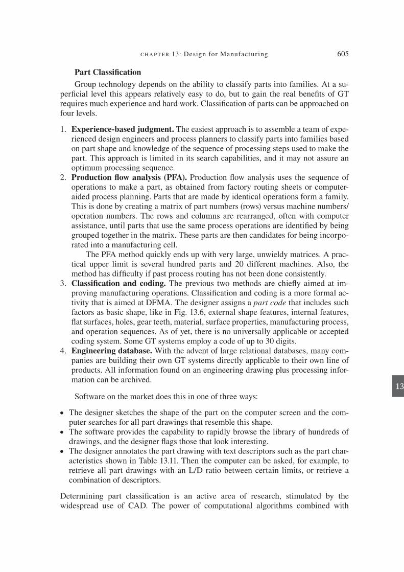
chapter 13: Design for Manufactur ing 605
13
Part Classid cation
Group technology depends on the ability to classify parts into families. At a su-per> cial level this appears relatively easy to do, but to gain the real bene> ts of GT requires much experience and hard work. Classi> cation of parts can be approached on four levels.
Experience-based judgment. The easiest approach is to assemble a team of expe-rienced design engineers and process planners to classify parts into families based on part shape and knowledge of the sequence of processing steps used to make the part. This approach is limited in its search capabilities, and it may not assure an optimum processing sequence. Production V ow analysis (PFA). Production R ow analysis uses the sequence of operations to make a part, as obtained from factory routing sheets or computer-aided process planning. Parts that are made by identical operations form a family. This is done by creating a matrix of part numbers (rows) versus machine numbers/operation numbers. The rows and columns are rearranged, often with computer assistance, until parts that use the same process operations are identi> ed by being grouped together in the matrix. These parts are then candidates for being incorpo-rated into a manufacturing cell.
The PFA method quickly ends up with very large, unwieldy matrices. A prac-tical upper limit is several hundred parts and 20 different machines. Also, the method has dif> culty if past process routing has not been done consistently. Classid cation and coding. The previous two methods are chieR y aimed at im-proving manufacturing operations. Classi> cation and coding is a more formal ac-tivity that is aimed at DFMA. The designer assigns a part code that includes such factors as basic shape, like in Fig. 13.6, external shape features, internal features, R at surfaces, holes, gear teeth, material, surface properties, manufacturing process, and operation sequences. As of yet, there is no universally applicable or accepted coding system. Some GT systems employ a code of up to 30 digits. Engineering database. With the advent of large relational databases, many com-panies are building their own GT systems directly applicable to their own line of products. All information found on an engineering drawing plus processing infor-mation can be archived.
Software on the market does this in one of three ways:
The designer sketches the shape of the part on the computer screen and the com-puter searches for all part drawings that resemble this shape.
The software provides the capability to rapidly browse the library of hundreds of drawings, and the designer R ags those that look interesting.
The designer annotates the part drawing with text descriptors such as the part char-acteristics shown in Table 13.11. Then the computer can be asked, for example, to retrieve all part drawings with an L/D ratio between certain limits, or retrieve a combination of descriptors.
Determining part classi> cation is an active area of research, stimulated by the widespread use of CAD. The power of computational algorithms combined with
1.
2.
3.
4.
●
●
●
die37039_ch13.indd 605 2/25/08 6:59:53 PM

606 engineering design
13
the capabilities of CAD systems assure that there will be continual improvement in the automation of part classi> cation.
13.8 MISTAKE-PROOFING
An important element of DFMA is to anticipate and avoid simple human errors that occur in the manufacturing process by taking preventive action early in the prod-uct design process. Shigeo Shingo, a Japanese manufacturing engineer, developed this idea in 1961 and called it poka-yoke .29 In English this is usually referred to as mistake-proo! ng or error proo! ng . A basic tenet of mistake-proo> ng is that human errors in manufacturing processes should not be blamed on individual operators but should be considered to be system errors due to incomplete engineering design. Mistake-proo> ng aims at reaching a state of zero defects, where a defect is de> ned as any variation from design or manufacturing speci> cation.
Common mistakes in manufacturing operations are:
Mistakes setting up workpieces and tools in machines or in > xtures Incorrect or missing parts in assemblies Processing the wrong workpiece Improper operations or adjustment of machines
Note that mistakes can occur not only in manufacturing but in design and purchasing as well. An infamous design mistake occurred with the 1999 orbiter to Mars, when it crashed on entering the Martian atmosphere. The contractor to NASA used conven-tional U.S. units instead of the speci> ed SI units in designing and building the control rockets, and the error was never detected by those who designed the control system in SI units.
13.8.1 Using Inspection to Find Mistakes
A natural response to eliminating mistakes is to increase the degree of inspection of parts by machine operators and of products by assembly line workers. However, as shown by Example 13.4, even the most rigorous inspection of the process output can-not eliminate all defects caused by mistakes.
E X A M P L E 1 3 . 4 Screening with Self-Checks and Successive Checks Assume a part is being made with a low average defect rate of 0.25% (0.0025). In an at-tempt to reduce defects even further, 100 percent inspection is employed. Each operator self-checks each part, and then the operator next in line checks the work of the previous operator.
A defect rate of 0.25% represents 2500 defects in each million parts produced (2500 ppm). If an operator has a 3% error rate in self inspection, and two operators inspect each part in succession, then the number of defective parts that pass through two successive
●
●
●
●
29 . Pronounced POH-kah YOH-kay.
die37039_ch13.indd 606 2/25/08 6:59:54 PM

chapter 13: Design for Manufactur ing 607
13
inspections is 2500(0.03)(0.03) 5 2.25 ppm. This is a very low level of defective parts. In fact it is below the magic percentage of defects of 3.4 ppm for achieving the Six Sigma level of quality (see Sec. 15.4).
However, the product is an assemblage of many parts. If each product consists of 100 parts, and each part is 999,998 ppm defect free, then a product of 100 parts has (0.999998) 100 or 999,800 ppm that are defect free. This leaves 200 ppm of assembled products that are defective. If the product has 1000 parts there would be 1999 defective products out of a million made. However, if the product has only 50 parts the defective products would decrease to 100 ppm.
This simple example shows that even with extreme and expensive 100 percent in-spection, it is dif> cult to achieve high levels of defect-free products, even when the prod-uct is not very complex. The example also shows that decreasing product complexity (part count) is a major factor in reducing product defects. As Shingo showed, 30 a different ap-proach from inspection is needed to achieve low levels of defects.
13.8.2 Frequent Mistakes
There are four categories of mistakes in part production. They are design mistakes, defective material mistakes, manufacturing mistakes, and human mistakes.
The following are mistakes attributable to the design process:
Providing ambiguous information on engineering drawings or speci> cations: Fail-ure to properly use GD&T dimensions and tolerances.
Incorrect information: Mistake in conversion of units or just plain wrong calculations.
A poorly developed design concept that does not fully provide the needed functional-ity. Hastily made design decisions that result in poorly performing products with low reliability, or with dangers to the safety of humans or hazards for the environment.
Defective material is another category of mistakes. These mistakes include:
Material that is poorly chosen because not all performance requirements have been considered in the selection. Most commonly these involve long-term properties such as corrosion or wear.
Material that does not meet speci> cations but gets into production, or purchased components that are not up to quality standards.
Parts with hard-to-detect R aws such as internal porosity or > ne surface cracks because of poorly designed dies or molds, or improper processing conditions (e.g., tempera-ture, rate of deformation, poor lubrication) for the material that is being processed.
The most common mistakes in manufacturing parts or their assembly are listed below, in decreasing order of frequency. 31
Omitted operations: Failure to perform a required step in the process plan. Omitted part: Forgetting to install a screw, gasket, or washer.
●
●
●
●
●
●
●
●
30. S . Shingo , Zero Quality Control: Source Inspection and the Poka-yoke System, Productivity Press, Portland, OR , 1986 . 31. C. M . Hinckley , Make No Mistake, Productivity Press, Portland, OR , 2000 .
die37039_ch13.indd 607 2/25/08 6:59:54 PM

608 engineering design
13
Wrong orientation of part: A part is inserted in the proper location but in the wrong orientation.
Misaligned part: Alignment is not suf> ciently accurate to give proper > t or function.
Wrong location of part: Part is oriented properly but in wrong location. Example: The short bolt is put in the location for the long bolt.
Selection of wrong parts: Many parts look very much alike. Example: A 1-inch bolt is used instead of 1¼ inch bolt.
Misadjustments: An operation is incorrectly adjusted. Commit a prohibited action: Often this is an accident, like dropping a wrench, or a safety violation, like failure to lock-out a power panel before hooking up a motor.
Added material or parts: Failure to remove materials. e.g., leaving on protective cover, or cores in a casting. Adding extra parts, e.g., dropping a screw into the assembly.
Misread, mismeasure, or misinterpret: Error in reading instruments, measuring di-mensions, or understanding correct information.
Some generic human mistakes, and safeguards that can be used against commit-ting these mistakes, are given in Table 13.12.
Constructive checking and correction, along with training and work standardiza-tion, are the best ways to limit human mistakes. However, the ultimate way to elimi-nate mistakes is to engineer them out of the system through improved product design and manufacturing. This process is outlined in Sec. 13.8.3.
13.8.3 Mistake-Prood ng Process
The steps in a mistake-proo> ng process follow a general problem-solving process:
Identify the problem. The nature of the mistake is not always obvious. There is a natural human tendency to conceal mistakes. Work hard to develop a culture of openness and quality consciousness. Normal inspection by sampling will not give suf> cient sample size of defects in a short time to identify the parts and processes causing the problem. Instead, use 100 percent inspection when looking for the cause of an error.
Prioritize. Once the sources of mistakes have been identi> ed, classify them with a Pareto chart to > nd the issues with the highest frequency of occurrence and which have the greatest impact on company pro> ts.
●
●
●
●
●
●
●
●
●
●
Table 13.12 Causes of Human Mistakes and Suggested Safeguards
Human Mistakes Safeguard
Inattentiveness Discipline; work standardization; work instructions
Forgetfulness Checking at regular intervals
Inexperience Skill enhancement; work standardization
Misunderstanding Training; checking in advance; standard work practices
Poor identi> cation Training; attentiveness; vigilance
die37039_ch13.indd 608 2/25/08 6:59:54 PM

chapter 13: Design for Manufactur ing 609
13
Use cause d nding methods. To identify the root cause of the mistake use the TQM tools of cause-and-effect diagram, why-why chart, and interrelationship digraph (presented in Sec. 4.7) to identify the root cause of the mistake.
Identify and implement solutions. General approaches for generating mistake-proo> ng solutions are discussed in Sec.13.8.4. Many solutions will reduce the defect rate in manufacturing parts and reduce the mistake rate in assembling the parts. However, the greatest impact will occur in the initial design of the part if DFMA guidelines are rigorously followed during embodiment design.
Evaluate. Determine if the problem has been solved. If the solution is ineffective, revisit the mistake-proo> ng process.
13.8.4 Mistake-Prood ng Solutions
In the broadest sense, mistake-proo> ng is about introducing controls to prevent mis-takes, detect mistakes, or detect defects arising from mistakes. Clearly it is better to prevent mistakes through appropriate design and operational controls than to only take action once a mistake has occurred.
Mistake-proo> ng operates in three areas of control.
Control of variability, as when a part diameter varies from piece to piece as parts are made in a manufacturing process. Control of variability is vital to making a quality product. This topic is covered in some detail in Chap. 15 under the topic of robust design.
Control of complexity is addressed chieR y through DFMA guidelines and can of-ten be traced back to issues arising with product architecture decisions in embodi-ment design.
Control of mistakes is implemented chieR y through the design and use of mistake-proo> ng devices 32 as were > rst suggested by the poka-yoke methodology.
Mistake-proo> ng devices can be grouped into > ve broad classi> cations:
Checklists. These are written or computer-based lists of process steps or tasks that need to be done for completeness of operation. The checklist that a commercial aircraft pilot goes through before take-off is a good example. To catch errors in operations, duplication of actions, as when you enter a computer password twice, is sometimes used. In manual assembly processes, instructions must be accompa-nied by clear pictures. Guide pins, guide ways, and slots. These design features are used in assembly to ensure that parts are located and oriented properly. It is important that guides should align parts before critical features mate. Specialized d xtures and jigs. These devices deal with a broader case of geom-etries and orientation issues. They typically are intended to catch any errors be-tween steps in the manufacturing process. Limit switches. Limit switches or other sensors detect mistakes in location, or the absence of a problem. These sensors trigger warnings, shut down the process,
●
●
●
●
●
●
1.
2.
3.
4.
32 . 200 examples of mistake-proo> ng devices are described in the Appendix A to C. M. Hinckley, op. cit.
die37039_ch13.indd 609 2/25/08 6:59:55 PM

610 engineering design
13
or enable it to continue. Sensors typically are interlocked with other processing equipment. Counters. Counters, either mechanical, electrical, or optical are used to verify that the proper number of machine operations or parts have been carried out. Tim-ers are used to verify the duration of a task.
Although the methods and examples of mistake-proo> ng have been given in the context of manufacturing processes, the methods can be implemented in areas such as sales, order entry, and purchasing, where the cost of mistakes is probably higher than the cost of errors that occur in manufacturing. A very similar, but more formalized process called Failure Modes and Effects Analysis (FMEA) is used to identify and improve upon potential failure modes in design; see Sec. 14.5.
13.9 EARLY ESTIMATION OF MANUFACTURING COST
The decisions about materials, shape, features, and tolerances that are made in the conceptual design and embodiment design phases determine the manufacturing cost of the product. It is not often possible to get large cost reductions once production has begun because of the high cost of change at this stage of the product life cycle. There-fore, we need a way of identifying costly designs as early as possible in the design process.
One way to achieve this goal is to include knowledgeable manufacturing personnel on the product design team. The importance of this is unassailable, but it is not always possible from a practical standpoint due to conR icts in time commitments, or even be-cause the design and manufacturing personnel may not be in the same location.
The method presented in Sec.13.4.6 is useful for selecting between alternative possible processes on the basis of estimated unit part cost. While considerable infor-mation is used, the level of detail is not suf> cient to do much better than give a relative ranking of competing manufacturing processes.
A system that is useful for cost estimation early in the design process was devel-oped at the University of Hull. 33 It is based on data obtained from British automotive, aerospace, and light manufacturing companies. It allows for the reasonable calcula-tion of part cost as changes are made in design details or for changes in part cost as different processes are used to manufacture the part. An important extension of the method in Sec. 13.4.6 is that the factor of part shape complexity is considered. Suf-> cient > gures are given below so that an example can be followed, but the book by Swift and Booker is required to obtain the full range of needed information. 34
The process starts with the identi> cation of a small number of materials and pro-cesses using Fig. 13.9. Comparison between alternatives is based on estimated unit manufacturing cost, C u .
5.
33. K. G . Swift and J. D . Booker, Process Selection, 2d ed., Butterworth-Heinemann, Oxford, UK , 2003 ; also A. J . Allen and K. G. Swift, Proc. Instn. Mech. Engrs., Vol. 204, pp. 143–48 , 1990 . 34 . The > gures in this section are from the > rst edition. They are used because the method can be shown with fewer > gures than the more expanded version in the second edition.
die37039_ch13.indd 610 2/25/08 6:59:55 PM

chapter 13: Design for Manufactur ing 611
13
CU 5 VCnn 1 PcRc (13.11)
Cnn 5 cost of material per unit volumeV 5 volume of material input to the process Pc 5 basic processing cost of an ideal part shapeRc = cost coef> cient for the part design that takes into account shape complex-
ity, material workability, section thickness, surface > nish, and tolerance.
Equation 13.11 shows that unit cost is estimated by > rst > nding the material cost and then adding the cost based on the general relationship between the process cost and the annual production volume, Fig. 13.16, for estimates of an “ideal” part design. This cost is then increased by all of the factors represented by Rc. The basic unit processing cost Pc is a composite cost representing capital equipment costs, operating costs (labor cost, and overhead), tooling cost, and rate of production. When plotted as in Fig. 13.16 it shows the basic relationship between the cost of different processes and the eco-nomic batch size for each process. These plots are based on average data for one shift per day and a 2-year payback for equipment and tooling.
The design-dependent factors are included in the R c term of Eq. (13.11).
Rc 5 Cmp 3 Cc 3 Cs 3 Cft (13.12)
where Cmp 5 relative cost associated with material-process suitability (workability or
fabricability)Cc 5 relative cost associated with shape complexityCs 5 relative cost associated with achieving minimum section thicknessCft 5 the higher of the costs to achieve a speci> ed surface > nish or tolerance, but
not both
For the design of the ideal part, each of the coef> cients in Eq. (13.12) is unity. As the design moves away from this situation, one or more of the coef> cients will increase in value, thereby increasing the unit manufacturing cost in Eq. (13.11).
Figure 13.17 shows the suitability rating of the material-process combinations that result in C mp . Note that many of the combinations are inadmissible for technical or economic reasons.
The shape complexity factor C c is based on the classi> cation system shown in Fig. 13.18. This system divides shapes into three basic categories: (A) solids of revolu-tion, (B) prismatic solids, and (C) R at or thin-wall section components. Within each category the complexity increases from 1 to 5. Shape classi> cation is based on the > n-ished shape of the part. C c is the most important coef> cient in Eq. (13.12). Therefore, careful study of the category de> nitions is important. Once the shape subcategory has been established, a set of curves for the process is entered (Fig. 13.19) and the coef> -cient is picked off. Figure 13.20 shows the curves for obtaining the section coef> cient C s . If the required section thickness falls to the left of the black vertical line, addi-tional secondary processing (machining or grinding) is likely to be necessary. This cost is included in the value of the coef> cient.
Curves for tolerances C t and surface > nish C f are given in Fig. 13.21. In using these charts, identify the most severe tolerance requirement in the part, and note
die37039_ch13.indd 611 2/25/08 6:59:55 PM

612 engineering design
13 whether it applies on one or more than one plane. The same applies for the surface > nish requirements. Note that the value for either C t or C f is used, depending on which coef> cient is larger. Costs estimated this way have been shown to be within at least 15 percent of the actual cost. Note that the Swift and Booker method uses a factor to ac-count for shape complexity, which is not considered at all in determining an estimate of manufacturing cost discussed in Sec.13.4.6.
E X A M P L E 1 3 . 5
We wish to estimate the cost of manufacturing the part shown at the top of A3 in Fig. 13.18. Its dimensions are as follows: large diameter 1 in. small diameter 0.25 in. length of long cylinder 2 in. length of short cylinder 1 in. The diameter of the cross-bore is such that the wall thickness is 5 mm. The tolerance on this bore diameter is 0.005 in. The sur-face > nish is 5 mm. We expect to need 10,000 parts per year. For strength reasons the part will be made from a quenched and tempered medium alloy steel.
3,0
00
,00
02
,00
0,0
00
1,0
00
,00
0
10
0,0
00
10
,00
0
10
00
10
0
10
0.1
1
10
100
Ba
sic
pro
ce
ssin
g c
ost
(Pc)
(pe
nce
)
1000
Quantity per annum (N)
10,000
50,000
Sheet metal-work
Impact extrusion
Pressure die
casting/injection molding
Automatic machine
Forging
Powder metallurgy
Manual
machine
Sand casting
FIGURE 13.16Average curves of P versus N for selected manufacturing processes. (From K. G. Swift and J. D. Booker, Process Selection, p. 175 Arnold, London. Used with permission.)
die37039_ch13.indd 612 2/25/08 6:59:56 PM

chapter 13: Design for Manufactur ing 613
13
Figure 13.9 suggests we look at whether the part should be made by sand casting, machining, or powder metallurgy. Using the charts reproduced in this section we estimate the coef> cients for Eq. (13.12) to be:
Process C mp C c C s C t C f R c P c P c R c
Sand casting 1.3 1.3 1.2 1.9 1.9 3.85 10.5 p 40 p
Machining 2.5 3.0 1.0 1.0 1.0 7.50 5 p 38 p
Powder metallurgy 1.1 2.4 1.0 1.0 1.0 2.64 60 p 158 p
FIGURE 13.17 Relative cost of material-process suitability, C mp . (From K. G . Swift , and J. D . Booker, Process Selection , p. 178, Arnold, London . Used with permission.)
Material
ProcessImpact
extrusion
Thermoplastic
Thermoset
Elastomers
1.1
1.2
1.1
1
1
1.5
Cast iron 1 1.2 1.6
Low carbon steel 1.3 1.2 1 1.2 1.4 1.2
Alloy steel 2 1.3 2 1.5 2.5 1.1
Stainless steel 2 1.5 2 1.5 4 1.1
Copper alloy 1 1 3 1 1 1.1 1
Aluminum alloy 1 1 1.5 1 1 1 1
Zinc alloy 1 1 1.2 1 1 1.1 1
Sand
casting
Pressure
die
casting
ForgingSheet
metal-
working
MachiningPowder
metallurgy
Injection
molding
Multiplying coef> cients according to Eq. (13.12) gives R c . Note how machining car-ries the greatest penalty because of the poor machinability of alloy steel and the geometry complexity. However, the basic processing cost P c is relatively low. The required number of parts is not suf> cient to pay back the tooling costs of powder metallurgy processing.
Turning now to Eq. (13.11), the volume of the part is 0.834 in 3 . The cost of alloy steel is about $1.25 per lb. Since the density of steel is 0.283 lb/in. 3 , C mv is $0.354 per in 3 and VC mv is $0.30. The rest of Eq. (13.11) is in pence ( p ). There are 100 pence to the pound (£), and l£ < $1.65. Therefore, VC mv 5 $0.30 /1.65 ($/£) 5 £0.182 5 18 p . The es-timated unit manufacturing cost is: sand casting 5 58 p ; machining 5 56 p , and powder metallurgy 5 176 p .
For this batch size machining is the preferred process over sand casting because the surface > nish and tolerances will be better. At 10,000 parts per year powder metallurgy is ruled out because of high tooling costs. However, experienced designers would have recognized that molding in a cross-bore is not good practice in powder metallurgy. The design guidelines in Table 13.3 should have warned us that a shape like A3 is not easily obtainable with powder metallurgy.
die37039_ch13.indd 613 2/25/08 6:59:56 PM
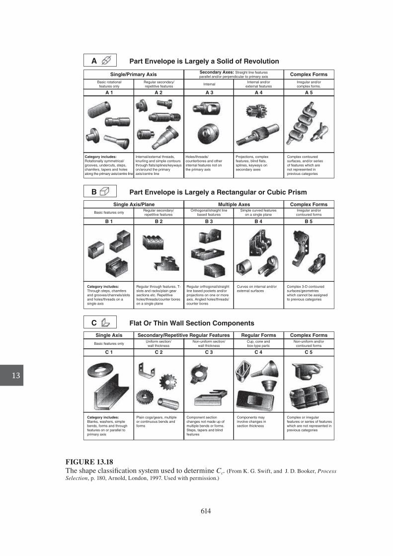
13
A Part Envelope is Largely a Solid of Revolution
Part Envelope is Largely a Rectangular or Cubic Prism
Flat Or Thin Wall Section Components
B
C
Category includes:
Rotationally symmetrical/
grooves, undercuts, steps,
chamfers, tapers and holes
along the primary axis/centre line
Internal/external threads,
knurling and simple contours
through flats/splines/keyways
on/around the primary
axis/centre line
Category includes:
Through steps, chamfers
and grooves/channels/slots
and holes/threads on a
single axis
Regular through features, T-
slots and racks/plain gear
sections etc. Repetitive
holes/threads/counter bores
on a single plane
Regular orthogonal/straight
line based pockets and/or
projections on one or more
axis. Angled holes/threads/
counter bores
Curves on internal and/or
external surfaces
Complex 3-D contoured
surfaces/geometries
which cannot be assigned
to previous categories
Holes/threads/
counterbores and other
internal features not on
the primary axis
Projections, complex
features, blind flats,
splines, keyways on
secondary axes
Complex contoured
surfaces, and/or series
of features which are
not represented in
previous categories
Single/Primary Axis Complex Forms
A 5A 1 A 4
Irregular and/or
complex forms.
Internal and/or
external featuresInternal
Regular secondary/
repetitive features
Basic rotational
features only
Secondary Axes: Straight line features
parallel and/or perpendicular to primary axis
A 3A 2
B 3 B 4 B 5B 2B 1
Multiple Axes Complex FormsSingle Axis/PlaneOrthogonal/straight line
based features
Simple curved features
on a single plane
Irregular and/or
contoured forms
Regular secondary/
repetitive featuresBasic features only
Category includes:
Blanks, washers, simple
bends, forms and through
features on or parallel to
primary axis
Plain cogs/gears, multiple
or continuous bends and
forms
Component section
changes not made up of
multiple bends or forms.
Steps, tapers and blind
features
Components may
involve changes in
section thickness
Complex or irregular
features or series of features
which are not represented in
previous categories
C 3 C 4 C 5C 2C 1
Secondary/Repetitive Regular Features Complex FormsRegular FormsSingle AxisNon-uniform section/
wall thickness
Cup, cone and
box-type parts
Non-uniform and/or
contoured forms
Uniform section/
wall thicknessBasic features only
FIGURE 13.18 The shape classi> cation system used to determine C c . (From K. G . Swift , and J. D . Booker, Process
Selection , p. 180, Arnold, London, 1997. Used with permission.)
614
die37039_ch13.indd 614 2/25/08 6:59:57 PM
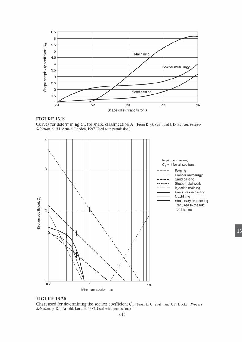
13
615
FIGURE 13.19Curves for determining Cc, for shape classi> cation A. (From K. G. Swift,and J. D. Booker, Process
Selection, p. 181, Arnold, London, 1997. Used with permission.)
A1 A2
Sh
ap
e c
om
ple
xity c
oe
ffic
ien
t, C
c
A3
Sand casting
Powder metallurgy
Machining
Shape classifications for ‘A’
A4 A51
1.5
2
2.5
3
3.5
4
4.5
5
5.5
6
6.5
FIGURE 13.20Chart used for determining the section coef> cient Cs. (From K. G. Swift, and J. D. Booker, Process
Selection, p. 184, Arnold, London, 1987. Used with permission.)
0.2 1
Minimum section, mm
Se
ctio
n c
oe
ffic
ien
t, C
s
1
2
3
4
10
Forging
Powder metallurgy
Sand casting
Sheet metal-work
Injection molding
Pressure die casting
Machining
Secondary processing
required to the left
of this line
Impact extrusion,
Cs = 1 for all sections
die37039_ch13.indd 615 2/25/08 6:59:57 PM

13
0.0
02
0.0
10
.1
To
lera
nce
, m
m
Sa
nd
Ca
stin
g
Tolerance coefficient, Ct
15
1
10
0.0
02
0.0
1
To
lera
nce
, m
m
Po
wd
er
Me
tallu
rgy
Tolerance coefficient, Ct
0.0
20
.03
1
10
0.0
02
0.0
10
.1
To
lera
nce
, m
m
Ma
ch
inin
g
Tolerance coefficient, Ct
0.2
1
10
0.1
10
Su
rfa
ce
fin
ish
,
mR
a!
Sa
nd
Ca
stin
g
Surface finish coefficient, Cf
15
01
10
0.1
Su
rfa
ce
fin
ish
,
mR
a!
Po
wd
er
Me
tallu
rgy
Surface finish coefficient, Cf
12
1
10
0.1
Su
rfa
ce
fin
ish
,
mR
a!
Ma
ch
inin
g
Surface finish coefficient, Cf
12
1
10
FIGURE 13.21 Charts used to determine C t (top row) and C f (bottom row). — 1 plane, —— 2 planes,——— 3 planes (From K. G . Swift, and J. D . Booker, Process Selection , Arnold, London, 1997. Used with permission.)
616
die37039_ch13.indd 616 2/25/08 6:59:57 PM

chapter 13: Design for Manufactur ing 617
13
13.10 COMPUTER METHODS FOR DFMA
The design for assembly methodology (DFA) was developed prior to formal DFM methodology, although DFM guidelines as “rules of thumb” have existed for centu-ries. DFA on the entire product assembly and its emphasis on reducing part count serves as a driver for DFM. DFM focuses more on the individual part and how to reduce the cost of manufacture. The objective is to quickly provide information on costs while the design is still R uid. While DFM and DFA methods can be done manu-ally on paper, the use of computerized methods greatly aids the designer by provid-ing prompts and help screens, providing access to data that is often scattered in the literature, and making it easy to quickly see the effect of design changes. The use of DFMA software also teaches good design practice. Whatever the method, a major bene> t from performing a DFMA analysis is that the rigor of using a formal analysis scheme invariably leads to asking better questions, and therefore to better solutions.
13.10.1 DFA Analysis
The most widely used design for assembly methodology is the Boothroyd-Dewhurst DFA method. 35 The method uses a step-by-step application of the DFA guidelines, like those given in Sec.13.6.1, to reduce the cost of manual assembly. The method is di-vided into an analysis phase and a redesign phase. In the > rst phase, the time required to handle and insert each part in the assembly is found from data tables based on time and motion study experiments. These values are derived from a part’s size, weight, and geometric characteristics. If the part requires reorienting after being handled, that time is also included. Also, each part is identi> ed as being essential or “theoretical,” (whether it is a candidate for elimination in a redesign phase). The decision on the minimum number of theoretical parts is determined by applying the criteria listed un-der Guideline 1 in Sec.13.6.1. Then the estimated total minutes to put together the as-sembly is determined. With this information the Design Assembly Ef> ciency can be determined using Eq. (13.10). This gives the designer an indication of how easily the design can be assembled, and how far the redesign phase should progress to increase assembly ef> ciency.
E X A M P L E 1 3 . 6
A design is needed for a motor-drive assembly that moves vertically on two steel guide rails. 36 The motor must be fully enclosed and have a removable cover for access to the po-sition sensor. The chief functional requirement is that there be a rigid base that supports the motor and the sensor and moves up and down on the rails. The motor must be fully enclosed and have a removable cover so the position detection sensor can be adjusted.
35. G. Boothroyd, P. Dewhurst and W. Knight, Product Design for Manufacture and Assembly, 2d ed., Marcel Dekker, New York, 2002. DFA and DFM software is available from Boothroyd-Dewhurst, Inc. www.dfma.com. 36. G . Boothroyd , “Design for Manufacture and Assembly,” ASM Handbook, Vol. 20, p. 676, ASM In-ternational, Materials Park, OH , 1997 .
die37039_ch13.indd 617 2/25/08 6:59:57 PM

618 engineering design
13 Figure 13.22 shows the initial design of the motor-drive assembly. The rigid base
is designed to slide up and down the steel guide rails (not shown). It also supports the linear motor and the position sensor. Two brass bushings are pressed into the base to provide suitable friction and wear characteristics for sliding on the steel rails. The end plate is > tted with a plastic grommet through which pass the connecting wires to the motor and the sensor. The box-shaped cover slides over the whole assembly from below the base and is held in place by four cover screws, two attached to the base and two passing into the end plate. In addition there are two stand-off rods that support the end plate and assorted screws to make a total of eight main parts and nine screws, for a total of 17 parts. The motor and sensor are outsourced subassemblies. The two guide rails are made from 0.5 in. diameter cold drawn steel bar stock. Because they are clearly essential components of the design, and there is no apparent substitute, they are not involved in the analysis.
We now use the DFA criteria to identify the theoretical parts, those that cannot be eliminated, and the parts that are candidates for replacement, Sec. 13.6.1.
Motor
(2.75 diam 3 4.75)
2 End-plate screws
(0.2 diam 3 0.5)
End plate (low-carbon steel,
painted, 4.5 3 2.25 3 1.3)
Grommet (plastic injection
molding, 0.7 diam 3 0.4)
2 Standoffs (low-carbon
steel, machined, 0.5 diam 3 2)
2 Bushings (brass, machined,
0.5 diam 3 0.8)
Base (aluminum,
machined, 4 3 2.2 3 1)
4 Cover screws
(0.12 diam 3 0.3)
Cover (16-gage low-carbon
steel with soldered seams
and painted, 4.5 3 2.75 3 2.4)
Set screw
(0.06 diam 3 0.12)
Sensor
(0.187 diam 3 1)
2 Motor screws
(0.2 diam 3 0.6)
FIGURE 13.22Initial design of the motor-drive assembly. (ASM Handbook, Vol. 20, p. 680, ASM Interna-tional, Materials Park, OH, 1997. Used with permission.)
die37039_ch13.indd 618 2/25/08 6:59:58 PM

chapter 13: Design for Manufactur ing 619
13
The base is clearly an essential part. It must move along the guide rails, which is a “given” for any redesign. However, by changing the material for the base from aluminum to some other material there could be a savings in part count. Aluminum sliding on steel is not a good combination. The bushings are part of the base and are included in the design to provide the function of low sliding friction. However, it is known that nylon (a thermoplastic polymer) has a much lower sliding coef> -cient of friction against steel than aluminum. Using nylon for the base would permit the elimination of the two brass bushings.
Now we consider the stand-off rods. We ask the question, “are they only there to connect two parts?” Since the answer is yes, they are candidates for elimination. However, if eliminated the end plate would have to be redesigned.
The end plate functions to protect the motor and sensor. This is a vital function, so the redesigned end plate is a cover and is a theoretical part. It must also be removable to allow access for servicing. This suggests that the cover could be a plastic molded part that would snap onto the base. This will eliminate the four cover screws. Since it will be made from a plastic, there is no longer a need for the grommet that is in the design to prevent fraying of the electrical leads entering the cover.
Both the motor and the sensor are outside of the part elimination process. They are clearly essential parts of the assembly, and their assembly time and cost of assem-bly will be included in the DFA analysis. However, their purchase cost will not be considered because they are purchased from outside vendors. These costs are part of the material costs for the product.
Finally, the set screw to hold the sensor in place and the two screws to secure the motor to the base are not theoretically required.
The time for manual assembly is determined by using lookup tables or charts 37 to estimate (1) the handling time, which includes grasping and orienting, and (2) the time for insertion and fastening. For example, the tables for handling time list different val-ues depending on the symmetry, thickness, size, and weight of the part, and whether it requires one hand or two to grasp and manipulate the part. Extra time is added for parts with handling dif> culties such as tangling, R exibility, or slipperiness, the need for optical magni> cation, or the need to use tools. For a product with many parts this can be a laborious procedure. The use of DFA software can be a substantial aid not only in reducing the time for this task, but in providing prompts and questions that as-sist in the decision process.
Tables for insertion time differentiate whether the part is secured immediately or whether other operations must take place before it can be secured. In the latter case it differentiates whether or not the part requires holding down, and how easy it is to align the part.
Table 13.13 shows the results of the DFA analysis of the initial design. As dis-cussed previously, the base, motor, sensor, and end plate are found to be essential parts, so the theoretical part count is 4 out of a total of 19 parts. Therefore, according to Eq. (13.10), the design ef> ciency for the assembly is quite low, 7.5 percent, indicat-ing that there should be ample opportunity for part elimination.
●
●
●
●
●
37. G. Boothroyd, et. al., op. cit., Chap. 3.
die37039_ch13.indd 619 2/25/08 6:59:58 PM

620 engineering design
13
In Table 13.13 the cost of assembly is determined by multiplying the total assem-bly time by the hourly cost of assembly. In this example it is $30/h.
The results of the DFA analysis for the redesigned motor-drive assembly, Fig. 13.23, are given in Table 13.14. Note that the part count has been reduced from 19 to 7, with an increase in the assembly ef> ciency from 7.5% to 26%. There is a com-mensurate reduction in the cost of assembly from $1.33 to $0.384. The three nonessen-tial parts are all screws that theoretically could be eliminated but have been retained for reliability and quality reasons. The next step is to do a design for manufacture analysis to determine whether the changes made in material and design have carried over to reduced part costs.
This example shows the importance of DFA in design. Even though assembly fol-lows part manufacturing, the DFA analysis contributes much more than reducing the cost of assembly, which rarely exceeds 20 percent of the product cost. A major contri-bution of DFA is that it forces the design team to think critically about part elimination through redesign. A part eliminated is a part that does not require manufacturing.
13.10.2 Concurrent Costing with DFM
The DFM Concurrent Costing software 38 allows the real-time cost estimation of parts using much more detail than the methods discussed previously in Sec. 13.4.6 and 13.9. Typically the program starts by downloading a CAD > le for the part that is to be
TABLE 13.13
Results of DFA Analysis for the Motor-Drive Assembly (Initial Design)
Part No. Theoretical Part Count
Assembly Time, s
Assembly Cost, ¢
Base 1 1 3.5 2.9
Bushing 2 0 12.3 10.2
Motor subassembly 1 1 9.5 7.9
Motor screw 2 0 21.0 17.5
Sensor subassembly 1 1 8.5 7.1
Setscrew 1 0 10.6 8.8
Stand-off 2 0 16.0 13.3
End plate 1 1 8.4 7.0
End-plate screw 2 0 16.6 13.8
Plastic bushing 1 0 3.5 2.9
Thread leads . . . . . . 5.0 4.2
Reorient . . . . . . 4.5 3.8
Cover 1 0 9.4 7.9
Cover screw 4 0 31.2 26.0
Total 19 4 160.0 133.0Design ef> ciency for assembly 5 (4 3 3)/160 5 7.5%
38 . Boothroyd-Dewhurst, Inc., www.dfma.com.
die37039_ch13.indd 620 2/25/08 6:59:58 PM
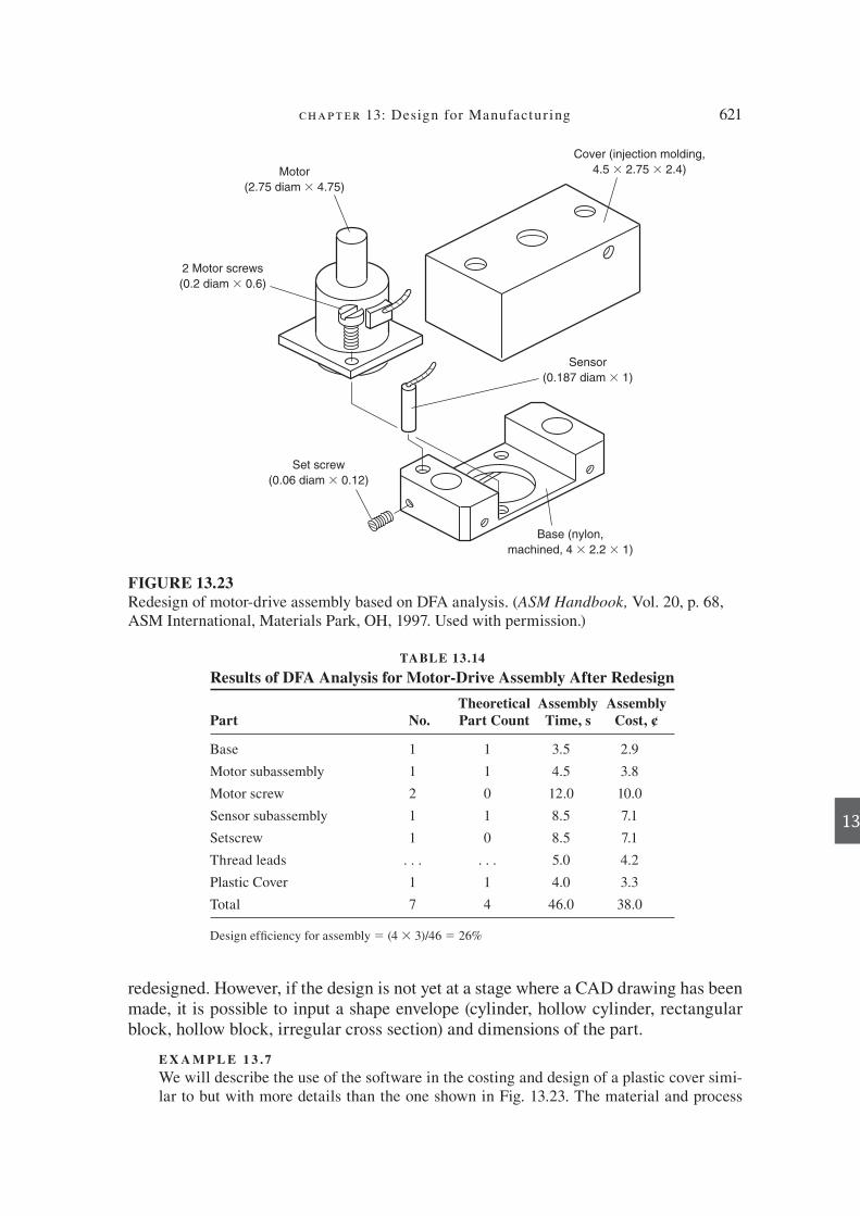
chapter 13: Design for Manufactur ing 621
13
redesigned. However, if the design is not yet at a stage where a CAD drawing has been made, it is possible to input a shape envelope (cylinder, hollow cylinder, rectangular block, hollow block, irregular cross section) and dimensions of the part.
E X A M P L E 1 3 . 7 We will describe the use of the software in the costing and design of a plastic cover simi-lar to but with more details than the one shown in Fig. 13.23. The material and process
FIGURE 13.23Redesign of motor-drive assembly based on DFA analysis. (ASM Handbook, Vol. 20, p. 68, ASM International, Materials Park, OH, 1997. Used with permission.)
Motor
(2.75 diam 3 4.75)
Cover (injection molding,
4.5 3 2.75 3 2.4)
Base (nylon,
machined, 4 3 2.2 3 1)
Set screw
(0.06 diam 3 0.12)
Sensor
(0.187 diam 3 1)
2 Motor screws
(0.2 diam 3 0.6)
TABLE 13.14
Results of DFA Analysis for Motor-Drive Assembly After Redesign
Part No. Theoretical Part Count
Assembly Time, s
Assembly Cost, ¢
Base 1 1 3.5 2.9
Motor subassembly 1 1 4.5 3.8
Motor screw 2 0 12.0 10.0
Sensor subassembly 1 1 8.5 7.1
Setscrew 1 0 8.5 7.1
Thread leads . . . . . . 5.0 4.2
Plastic Cover 1 1 4.0 3.3
Total 7 4 46.0 38.0
Design ef> ciency for assembly 5 (4 3 3)/46 5 26%
die37039_ch13.indd 621 2/25/08 6:59:59 PM

622 engineering design
13
are selected from drop-down menus. Generally this starts with a menu of materials and processes, and selection of a class of materials gives the designer the option of selecting a speci> c material. Selecting the material greatly limits the choice of processes. Injection molding is the obvious choice for the hollow rectangle made from the thermoplastic ABS.
Figure 13.24 shows the computer screen after the material and process have been selected. The values are determined by the part geometry that is entered as a drawing, and default values for the injection molding process. Because this is a molding process, much of the cost is determined by the cost of the mold. The DFM input will be concerned chieR y with how decisions on design details are reR ected in the cost to make the tooling.
Following down the list of design parameters we come to part complexity. Part com-plexity is measured by the number of surface patches needed to describe both the inner and outer surface of the part. The inner surface of the cover is ribbed and contains bosses used for making screw connections, so the patches add up to a considerable value. The next two sections ask for input that further de> nes the mold cost.
Tolerances: The tightness of the tolerance determines the care needed in machining the mold cavity.
Appearance: If the part is transparent, the mold surface will need to be polished to a high degree.
Texture: If the surface needs to have a grain or leather appearance, this will require > ne engraving of the mold surface.
Parting line: The parting line refers to the shape of the surface across which the mold separates to eject the part. A straight parting plane is the least costly, but if the part design requires a stepped or curved surface, the mold cost will be signi> cantly increased.
Mold construction: A two-plate mold, a stationary cavity plate, and a moving core plate is the least complex mold system.
Runner system: For high rates of production a heated runner is designed into the > xed plate. This also eliminates the need to separate the runners and sprues from the part. This mold feature adds cost to the mold.
Mold material: This choice will determine the life of the mold. Number of cavities: Depending on the size of the part, it is possible to make more than
one part per shot. This requires several cavities, which increases the productivity, . n,
but also increases the machining time and the mold cost. Devices in one cavity: If it is necessary to mold depressions or undercuts on the inside
of the part, it requires building the core pin retraction device inside the core plate. This is dif> cult and very expensive.
Users of the software need some knowledge of the construction and operation of injection molds to go beyond the basic default values and link the part design with mold construc-tion costs. 39
Note that the preliminary piece part cost and the tooling cost allocated to each part are given at the bottom left in Fig. 13.24. Any of the parameters in this table can be changed, and the costs will be recalculated quickly to show the effect of the change. For example, we might decide that using 30 percent of recycled (regrind) plastic resin would degrade the properties of the part, so this value is set at 10 percent. This change increases the material cost. Next, we decide that the part size is small enough that two parts can be made in a single mold. The number of cavities is changed from 1 to 2. This increases the
●
●
●
●
●
●
●
●
●
39. G . Boothroyd , et. al., op. cit., Chap. 8; H . Rees and B . Catoen , Selecting Injection Molds, Hanser Gardner Publications, Cincinnati, OH , 2005 .
die37039_ch13.indd 622 2/25/08 6:59:59 PM
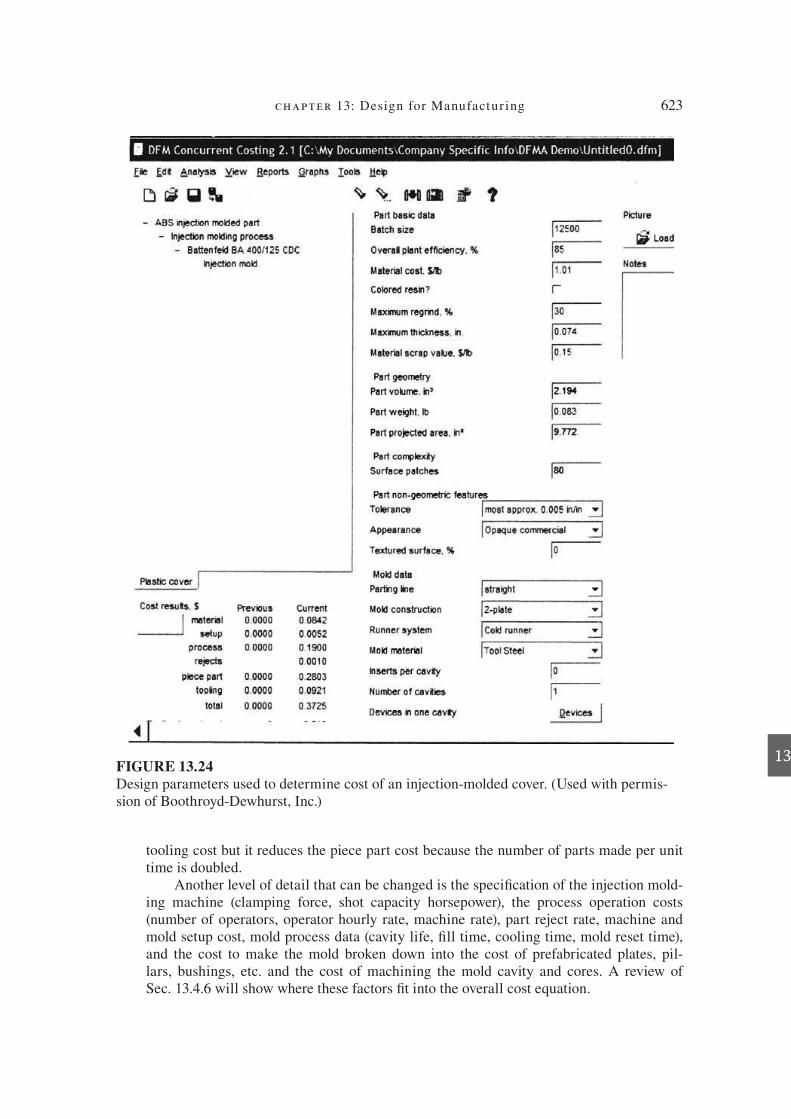
chapter 13: Design for Manufactur ing 623
13
tooling cost but it reduces the piece part cost because the number of parts made per unit time is doubled.
Another level of detail that can be changed is the speci> cation of the injection mold-ing machine (clamping force, shot capacity horsepower), the process operation costs (number of operators, operator hourly rate, machine rate), part reject rate, machine and mold setup cost, mold process data (cavity life, > ll time, cooling time, mold reset time), and the cost to make the mold broken down into the cost of prefabricated plates, pil-lars, bushings, etc. and the cost of machining the mold cavity and cores. A review of Sec. 13.4.6 will show where these factors > t into the overall cost equation.
FIGURE 13.24 Design parameters used to determine cost of an injection-molded cover. (Used with permis-sion of Boothroyd-Dewhurst, Inc.)
die37039_ch13.indd 623 2/25/08 6:59:59 PM

624 engineering design
13
This example shows the level of detail that is needed for a reliable determination of part cost, especially the cost of tooling and process operations. The degree of de-sign complexity and interaction with process parameters is such that a computer-based cost model is the only way to do this quickly and consistently. Design details made at the con> guration design step can be explored in a “what-if” mode for their impact on tooling costs before an actual commitment to purchase tooling is made. The sections that follow give more information on design details pertinent to particular processes.
13.10.3 Process Modeling and Simulation
Advances in computer technology and > nite element analysis have led to industry’s widespread adoption of computer process models. Just as > nite element and > nite difference analyses and CFD have made possible re> ned design for performance of components that have reduced the cost of prototype testing, so have computer process models 40 reduced the development time and cost of tooling. The greatest application of process models has been with casting, injection molding, closed-die forging, and sheet metal forming processes.
Since most manufacturing processes use large equipment and expensive tooling, it is costly and time consuming to do process improvement development. A typical type of problem is making re> nements to the mold to achieve complete material R ow in all regions of a component made by casting or injection molding. In deformation processes like forging or extrusion, a typical problem is to modify the dies to prevent cracking in regions of high stress in the part. Today, these types of problems and many others can be solved quickly using commercially available simulation software. The results of the analysis can be seen as a series of color maps of a process parameter, such as tempera-ture. Animations showing the actual solidi> cation of the metal over time are common-place. References to common process modeling software will be given as we describe the DFM guidelines for several processes in subsequent sections of this chapter.
13.11DESIGN OF CASTINGS
One of the shortest routes from raw material to > nished part is a casting process. In casting, a molten metal is poured into a mold or cavity that approximates the shape of the > nished part (Fig. 13.25). Heat is extracted through the mold (in this case a sand mold), and the molten metal solidi> es into the > nal solid shape. The chief design issues for the mold are (1) to provide an entry for the molten metal into the mold that creates laminar R ow through the sprue and runner, (2) to provide a source of molten metal, suitably located in the mold so that it stays molten until all of the casting has been > lled, and (3) that cores are suitably placed to provide hollow features for the part.
40. J. A. Dantzig, and C. T. Tucker III, Modeling in Materials Processing, Cambridge University Press, Cambridge, UK, 2001.
die37039_ch13.indd 624 2/25/08 7:00:00 PM
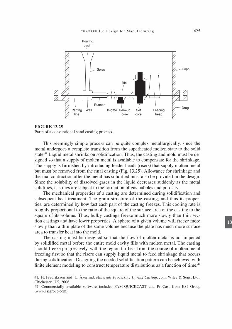
chapter 13: Design for Manufactur ing 625
13
This seemingly simple process can be quite complex metallurgically, since the metal undergoes a complete transition from the superheated molten state to the solid state. 41 Liquid metal shrinks on solidi> cation. Thus, the casting and mold must be de-signed so that a supply of molten metal is available to compensate for the shrinkage. The supply is furnished by introducing feeder heads (risers) that supply molten metal but must be removed from the > nal casting (Fig. 13.25). Allowance for shrinkage and thermal contraction after the metal has solidi> ed must also be provided in the design. Since the solubility of dissolved gases in the liquid decreases suddenly as the metal solidi> es, castings are subject to the formation of gas bubbles and porosity.
The mechanical properties of a casting are determined during solidi> cation and subsequent heat treatment. The grain structure of the casting, and thus its proper-ties, are determined by how fast each part of the casting freezes. This cooling rate is roughly proportional to the ratio of the square of the surface area of the casting to the square of its volume. Thus, bulky castings freeze much more slowly than thin sec-tion castings and have lower properties. A sphere of a given volume will freeze more slowly than a thin plate of the same volume because the plate has much more surface area to transfer heat into the mold.
The casting must be designed so that the R ow of molten metal is not impeded by solidi> ed metal before the entire mold cavity > lls with molten metal. The casting should freeze progressively, with the region farthest from the source of molten metal freezing > rst so that the risers can supply liquid metal to feed shrinkage that occurs during solidi> cation. Designing the needed solidi> cation pattern can be achieved with > nite element modeling to construct temperature distributions as a function of time. 42
FIGURE 13.25Parts of a conventional sand casting process.
Sprue
Rib
Pouring
basin
Parting
line
Well
Runner
In-gate Ram-up
core
Set
core
Feeding
head
Drag
Cope
41. H . Fredriksson and U . Åkerlind , Materials Processing During Casting, John Wiley & Sons, Ltd., Chichester, UK , 2006 . 42 . Commercially available software includes PAM-QUICKCAST and ProCast from ESI Group (www.esigroup.com).
die37039_ch13.indd 625 2/25/08 7:00:00 PM

626 engineering design
13
The FEA can predict shrinkage regions due to lack of feeding and grain size (prop-erty) distribution in the casting.
There are a large number of casting processes, which can be classi> ed best with respect to the type of mold that is employed (Fig. 13.26). The two broad categories are expendable mold casting, in which the mold is destroyed after making each part, and permanent mold casting , for which many parts are made in each mold. A brief description of each process is given at www.mhhe.com/dieter.
13.11.1 Guidelines for the Design of Castings
Proper attention to design details can minimize casting problems and lead to lower costs. 43 Therefore, close collaboration between the designer and the foundry engineer is important. The use of computer-based solidi> cation modeling in this design col-laboration is recommended.
The chief consideration is that the shape of the casting should allow for orderly solidi> cation by which the solidi> cation front progresses from the remotest parts to-ward the points where molten metal is fed in. Whenever possible, section thickness should be uniform. Large masses of metal lead to hot spots, where freezing is delayed, and a shrinkage cavity is produced when the surrounding metal freezes > rst.
Figure 13.27 illustrates some design features that can eliminate the shrinkage cavity problem. A transition between two sections of different thicknesses should be made gradually (a). As a rule of thumb, the difference in thickness of adjoining sec-tions should not exceed 2 to 1. Wedge-shaped changes in wall thickness should not have a taper exceeding 1 to 4. The thickness of a boss or pad (b) should be less than the thickness of the section the boss adjoins, and the transition should be gradual. The local heavy section caused by omitting the outer radius at a corner (c) should be elimi-nated. The radius for good shrinkage control should be from one-half to one-third of
FIGURE 13.26Classi> cation of casting processes.
Casting processes
Expendable mold
Permanent pattern Expendable pattern
Permanent mold
Sand moldingGreenCO2
Investment casting
Permanentmold casting
Shell molding Resin
MetalGraphite
Plaster mold
Die casting
Centrifugal casting
43. Casting Design Handbook, American Society for Metals, 1962; ASM Handbook , Vol. 15, American Society for Metals, Materials Park, OH , 1988 ; T. S . Piwonka , “Design for Casting,” ASM Handbook , Vol. 20, pp. 723–29 , ASM International, Materials Park, OH , 1997 .
die37039_ch13.indd 626 2/25/08 7:00:00 PM

chapter 13: Design for Manufactur ing 627
13
the section thickness. A strong hot spot is produced when two ribs cross each other (d). These areas solidify after the thinner sections surrounding the junction so that the shrinkage cannot be fed with liquid metal, resulting in a shrinkage cavity. This prob-lem can be eliminated by offsetting the ribs as shown in (d). A good way to evaluate where hot spots brought about by a large mass of molten metal, occur is to inscribe a circle in the cross section of the part. The larger the diameter of the circle, the greater the thermal mass effect, and the more the concern with shrinkage cavity formation.
Castings must be designed to ensure that the pattern can be removed from the mold and the casting from a permanent mold. A draft , or taper, of from 6 to 3 degrees is required on vertical surfaces so the pattern can be removed from the mold. Project-ing details or undercuts should be avoided, as these require extra cores. Molds made with extensive use of cores cost more money, so castings should be designed to mini-mize the use of cores. Also, provisions must be made for placing cores in the mold cavity and holding them in place when the metal R ows into the mold.
Solidi> cation stresses can occur when different sections of the casting solidify at different times and rates. If this happens while the alloy is cooling through the tem-perature range where both liquid and solids coexist, it can result in internal fracture called hot tearing . Uneven cooling as the temperature continues to drop can result in severe distortion or warping of the casting.
Some casting processes like die casting, permanent mold casting and investment casting produce parts with excellent dimensional accuracy and smooth surfaces. Parts made with these processes are net shape parts that require no machining before using. Sand-cast parts always require machining after casting in order to attain the required dimensions and surface > nish. Therefore, it is necessary to provide extra material in the casting as a machining allowance .
13.11.2 Producing Quality Castings
Casting offers exceptional design R exibility of shape at reasonable cost. It is an an-cient metalworking process that has not always enjoyed a reputation for producing high-quality parts. A point not always understood by designers is that in a part made by casting, its mechanical properties depend on the design of the part because the properties depend on the size and shape of the grains. This depends on the solidi> ca-tion rate, which in turn depends on the thickness of different sections of the part. Fur-thermore, most casting processes are carried out in the atmosphere so that hot liquid metal can react with air to form oxide > lms and inclusions. Inclusions are nonmetallic particles formed by interaction with the mold or from chemical reactions among the constituents of the molten metal. These can serve as sites for crack initiation, and oxide > lms themselves can act like cracks.
Porosity of various origins can be present in a cast part. We have already dis-cussed the macroporosity 44 produced by inadequate feeding of liquid while the cast-ing is cooling. This is solved by modi> cations to the part geometry combined with better placement of risers in the casting. The use of solidi> cation computer models is
44 . Macroporosity is large enough to be seen with the unaided eye on radiographic inspection. Micropo-rosity refers to pores that are not visible without magni> cation.
die37039_ch13.indd 627 2/25/08 7:00:01 PM

628 engineering design
13
highly effective in identifying possible sites for macroporosity. The second type of po-rosity, microporosity, is more dif> cult to eliminate. As the metal solidi> es it tends to form small, interlocking, tree-like structures called dendrites. When these approach 40 percent solid material by volume, the passages for further R uid inR ow become blocked, leaving a > ne porosity network. A second mechanism for pore formation arises from the fact that the solubility of gases in liquid metal decreases strongly with falling temperature. Thus, the dissolved gases are expelled from the liquid metal, and they form bubbles that grow into sizeable pores.
Microporosity can be minimized by the choice of alloy, but it is not something the designer can affect by the part design. It can be nearly eliminated by melting and pouring in the absence of air (vacuum melting), as is done for aircraft turbine blades, but this is very expensive. Another possibility is to use hot isostatic pressing (HIP) to close up any residual porosity. This process consists of enclosing the parts in a pres-sure vessel and subjecting them to a hydrostatic pressure of argon at 15 to 25 ksi at an elevated temperature for several hours. This will eliminate nearly all vestiges of microporosity, but again it is not an inexpensive secondary process.
The complexity of successfully casting parts with high-quality metallurgical properties requires the designer to be able to predict the solidi> cation of the part and the metallurgical structure of the > nal part. At a minimum this means being able to determine how the part will solidify before a casting is poured, and to make design alterations until a casting is obtained without macroporosity. It would be highly desir-able to be able to map the temperature-time curve at critical points in the casting. To do this requires teaming up with a progressive foundry with an experienced foundry engineer who is skilled in using solidi> cation software. The most advanced software is capable of predicting grain size and structure, and therefore being able to infer mechanical properties. This software is also capable of predicting the distortions that occur during casting.
FIGURE 13.27Some design details to minimize shrinkage cavity formation.
Poor
Shrinkage
cavity
Poor
GoodGood
Poor
Good
Poor
Good
(d)(b) (c)(a)
die37039_ch13.indd 628 2/25/08 7:00:01 PM
chapter 13: Design for Manufactur ing 629
13
Obtaining quality castings requires working with a foundry that is up-to-date on the latest casting technology. 45 Much of this newer technology deals with minimizing defects in castings. A high-tech foundry will be knowledgeable about and practicing such things as:
The proper way to prepare the melt to minimize the level of inclusions and level of dissolved gas
Design of sprue, runner, and ingate so as to minimize the distance the liquid metal falls or prevent molten metal from spilling into un> lled regions of the casting
Mold design to keep the liquid metal front moving at all times Design to eliminate bubbles of entrained air in the liquid metal Design to avoid the need to feed metal uphill against gravity Finding out whether feeding requirements are established by calculation or guesswork
Design to prevent convection problems by ensuring that thermal gradients act with rather than against gravity
The use of > lters to reduce inclusions in the casting
This knowledge area is not that of the part designer, but he should at least be aware of the issues so as to be able to evaluate the technical capability of his casting supplier.
Using casting simulation software to design the part and mold, and using a part supplier that employs modern casting operations concepts, will produce parts that per-form admirably in many applications. Reducing the level of defects will result in parts with more reproducible mechanical properties than are usually expected from castings. This is important in allowing designers to gain con> dence that castings can be used in applications where forgings were previously the process of choice. This has happened in aircraft engine applications like jet turbine blades, where the highly alloyed metals needed to resist creep at high temperatures are very dif> cult to shape by deformation processes like forging. The quality casting technology that has been developed for these types of applications is > nding its way into less demanding applications.
13.12 DESIGN OF FORGINGS
Forging processes are among the most important means of producing parts for high- performance applications. Forging is typical of a group of bulk deformation processes in which a solid billet is forced under high pressure by the use of a press to undergo extensive plastic deformation into a > nal near-to-> nished shape. 46 Other examples of deformation processes are extrusion , in which a long object with a high L/D ratio is produced by pushing a metal billet through a die, drawing , in which a billet is pulled through a die, and rolling, in which a slab is passed through rolls to make a thin sheet.
●
●
●
●
●
●
●
●
45. M . Jolly , “Professor John Campbell’s Ten Rules for Making Reliable Castings,” JOM , May 2005, pp. 19–28; J . Campbell , Castings Practice: The Ten Rules of Castings, 2d ed., Butterworth-Heinemann, Oxford, UK , 2004 . 46. B. L . Ferguson , “Design for Deformation Processes,” ASM Handbook, Vol. 20, pp. 730–44 , ASM International, Materials Park, OH , 1997 . To see animations of various types of forging processes, go to www.deform.com and click on Applications.
die37039_ch13.indd 629 2/25/08 7:00:01 PM

630 engineering design
13
Forging usually is carried out on a hot workpiece, but other deformation pro-cesses such as cold extrusion or impact extrusion may be conducted cold, depending upon the material. Because of the extensive plastic deformation that occurs in forging, the metal undergoes metallurgical changes. Any porosity is closed up, and the grain structure and second phases are deformed and elongated in the principal directions of working, creating a “> ber structure.” The forging billet has an axial > ber structure due to hot working, but this is redistributed depending upon the geometry of the forg-ing (Fig. 13.28).
The mechanical > bering due to the preferred alignment of inclusions, voids, segre-gation, and second-phase particles in the direction of working introduces a direction-ality (anisotropy) to structure-sensitive properties such as ductility, fatigue strength, and fracture toughness. The principal direction of working (such as the long axis of a bar) is de> ned as the longitudinal direction. The long-transverse direction is perpen-dicular to the longitudinal direction. The variation of reduction of area in the tensile test (the most sensitive measure of ductility) with the angle that the specimen axis makes with the forging axis is shown in Fig. 13.29. This shows that structure-sensitive mechanical properties like reduction of area, fatigue limit, and fracture toughness ex-hibit anisotropy as a result of closing up of porosity and alignment of second-phase particles produced by the plastic deformation. The designer needs to realize that some properties may not be the same in all directions of the forging. Therefore, in design-ing a forging, the direction of maximum plastic deformation (longitudinal) should be aligned with the direction of the part that needs to carry the maximum stress.
Forgings are classi> ed into open- or closed-die forgings. Open dies, usually R at dies, are used to impose localized forces for deforming billets progressively into simple shapes, much as the blacksmith does with his hammer and anvil. Closed-die forging or impression die forging uses mechanical presses or hammers to force the metal to R ow into a closed cavity to produce complex shapes to close dimensional tolerances. A wide variety of shapes, sizes, and materials can be made in forging. Table describing the advantages of the common forging processes can be found at www.mhhe.com/dieter. With proper forging die design, grain R ow is controlled to give the best properties at the critically stressed regions.
FIGURE 13.28The redistribution of the > ber structure direction during the forging of a part.
Original
billet
Forged
blank
die37039_ch13.indd 630 2/25/08 7:00:02 PM
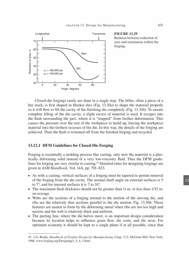
chapter 13: Design for Manufactur ing 631
13
Closed-die forgings rarely are done in a single step. The billet, often a piece of a bar stock, is > rst shaped in blocker dies (Fig. 13.30 a ) to shape the material properly so it will R ow to > ll the cavity of the > nishing die completely (Fig. 13.30 b ). To ensure complete > lling of the die cavity, a slight excess of material is used. It escapes into the R ash surrounding the part, where it is “trapped” from further deformation. This causes the pressure over the rest of the workpiece to build up, forcing the workpiece material into the farthest recesses of the die. In this way, the details of the forging are achieved. Then the R ash is trimmed off from the > nished forging and recycled.
13.12.1 DFM Guidelines for Closed-Die Forging
Forging is essentially a molding process like casting, only now the material is a plas-tically deforming solid instead of a very low-viscosity R uid. Thus the DFM guide-lines for forging are very similar to casting. 47 Detailed rules for designing forgings are given in ASM Handbook, Vol. 14A, pp. 701–823.
As with a casting, vertical surfaces of a forging must be tapered to permit removal of the forging from the die cavity. The normal draft angle on external surfaces is 5 to 7°, and for internal surfaces it is 7 to 10°.
The maximum R ash thickness should not be greater than ¼ in. or less than 1/32 in. on average.
Webs are the sections of a forging normal to the motion of the moving die, and ribs are the relatively thin sections parallel to the die motion, Fig. 13.30 b . These features are easiest to form by the deforming metal when ribs are not too high and narrow and the web is relatively thick and uniform.
The parting line, where the die halves meet, is an important design consideration because its location helps to inR uence grain R ow, die costs, and die wear. For optimum economy it should be kept to a single plane if at all possible, since that
●
●
●
●
47. J. G . Bralla , Handbook of Product Design for Manufacturing, Chap. 3.13, McGraw-Hill, New York , 1986 ; www.forging.org\Design\pg3_5_4_1.html
FIGURE 13.29Relation between reduction of area and orientation within the forging.
Longitudinal Transverse
Max
Min
Re
du
ctio
n o
f a
rea
, %
0 20 4020
30
40
50
60
70
Angle, degrees
#u = 166,000 psi
0 = 146,000 psi
60 80
die37039_ch13.indd 631 2/25/08 7:00:02 PM

632 engineering design
13
will make die sinking, forging, and trimming less costly. Figure 13.30 shows that the C ash occurs at the parting line. Because the forging F ber structure is unavoid-ably cut through when the C ash is trimmed, the parting line is best placed where the minimum stresses arise in the service of the forging.
Whenever possible in the design of forgings, as in the design of castings, it is desir-able to keep the thickness of adjacent sections as uniform as possible. Rapid changes in section thickness should be avoided. Laps 48 and cracks are most likely to occur where metal C ow changes because of large differences in the bulk of the sections. To prevent these defects, generous radii must be provided at those locations.
Most forging is done at elevated temperature where the C ow (yield) stress of the material is much lower than at room temperature. This signiF cantly reduces the pressure that must be produced in the dies, but it also causes oxidation of the sur-face. The machining envelope is the excess metal that must be removed to bring the forging to the F nished size and surface F nish. The ultimate in precision forg-ing is the net-shape forging , in which the machining allowance is zero. Generally, however, allowance must be made for removing surface scale (oxide), correcting for warpage and mismatch (where the upper and lower dies shift parallel to the parting plane), and for dimensional mistakes due to thermal contraction or die wear.
13.12.2 Computer-Aided Forging Design
To predict the sequence of shapes to go from a piece of bar stock to a complex, defect-free forged shape requires great skill on the part of the die designer. This complex engineering task has been greatly aided by 30 years of research in applying FEA to
●
●
3 to 5°7 to 10°
Land
Flash
gutter
R
Rb
h
Flash
FIGURE 13.30
Schematic of closed-die forging. (a) Blocker die; (b) F nishing die. (After J.A. Schey.)
48 . A lap is a surface defect caused by metal being forded over and then forged into the surface without being welded. Laps often cause fatigue cracks.
die37039_ch13.indd 632 2/25/08 7:00:03 PM

chapter 13: Design for Manufactur ing 633
13
the analysis of deformation processes. Currently, software is available for the desktop computer 49 that allows the designer to accurately determine not only press loads and die stresses but also such signiF cant parameters as stress, strain, and temperature dis-tribution throughout the deforming workpiece and free surface proF le. An important feature of the software is the ability to visualize the geometrical changes in the work-piece as the dies close in each step of the process. The designer can make changes in the tooling design and observe on subsequent simulations whether these led to im-provement in the material C ow and eliminated C ow defects like laps or incomplete die F ll. The savings in the cost of reworking dies and trying out reworked dies have led to broad industry adoption of deformation processing simulation software. Comple-mentary software models the change in grain size as the part undergoes forging at elevated temperature.
13.13 DESIGN FOR SHEET-METAL FORMING
Sheet metal is widely used for industrial and consumer parts because of its capacity for being bent and formed into intricate shapes. Sheet-metal parts comprise a large fraction of automotive, agricultural, and aircraft components. Successful sheet-metal forming depends on the selection of a material with adequate formability, the proper design of the part and the tooling, the surface condition of the sheet, the selection and application of lubricants, and the speed of the forming press.
13.13.1 Sheet Metal Stamping
The cold stamping of a strip or sheet of metal with dies can be classiF ed as either a cutting or a forming operation. 50 Cutting operations are designed to punch holes in sheets or to separate entire parts from sheets by blanking . A blanked shape may be either a F nished part or the F rst stage in a forming operation in which the F nal shape is created by plastic deformation.
The sheared edge that is produced when sheet metal is punched or blanked is neither perfectly smooth nor perpendicular to the sheet surface. Simple blank contours should be used whenever possible since the die cost depends upon the length and the intricacy of the contour of the blank. It may be less expensive to construct a compo-nent from several simple parts than to make an intricate blanked part. Blanks with sharp corners are expensive to produce. The layout of the blanks on the sheet should be such as to minimize scrap loss.
Notching a blank along one edge results in an unbalanced force that makes it dif-F cult to control dimensions as accurately as with blanking around the entire contour. The usual tolerances on blanked parts are !0.003 in.
49 . DEFORM® from ScientiF c Forming Technologies, Columbus, OH. 50. ASM Handbook, Vol.14B, Metalworking: Sheet Forming, ASM International, Materials Park, OH , 2006 ; J. A . Schey , Introduction to Manufacturing Processes, 3d ed., Chap. 10, McGraw-Hill, New York , 2000 .
die37039_ch13.indd 633 2/25/08 7:00:03 PM

634 engineering design
13
When holes are punched in metal sheet, only part of the metal thickness is sheared cleanly; that is, a hole with partially tapered sides is created. If the hole is to be used as a bearing surface, then a subsequent operation will be required to obtain parallel walls. Diameters of punched holes should not be less than the thickness of the sheet or a minimum of 0.025 in. Smaller holes result in excessive punch breakage and should be drilled. The minimum distance between holes, or between a hole and the edge of the sheet, should be at least equal to the sheet thickness. If holes are to be threaded, the sheet thickness must be at least one-half the thread diameter.
13.13.2 Sheet Bending
Bending is a common sheet-forming operation. Bending along a straight line is done by wiping , Fig. 13.31a . The sheet is held down with a pressure pad and is wiped over the die radius with a wiping die. Long, straight bends are made in a press-brake, which is a type of press in which the sheet is placed between two dies. Thick sheet and plate are bent using a three-roll bender, Fig. 13.31b . The radius of curvature of the bend can be changed by varying the distance between the rolls. Long shapes like garage door channels are made by roll forming.
A sheet metal part that is bent must undergo plastic deformation if it is to re-tain its bent shape. When this happens the bend region elongates a small amount and the sheet thins slightly to maintain a constant volume. The bend allowance, LBA , the length of the neutral axis in the bend, is given by
L R ktBA b
= +( )α (13.13)
where a is the bend angle in radians, R b is the bend radius (measured to the inside of the bend), and t is the thickness of the sheet. If R b .2t the neutral axis is in the center of the sheet thickness and k 5 0.5. However, if R b ,2t (a sharp bend) the neutral axis is located about one-third of the distance from the inner bend surface, k 5 0.33.
Pressure
Pad Wiping
die
Adjust for
curvature
Die
RR
h
FIGURE 13.31
Sheet bending with a (a) wiping die, and (b) bending rolls.
die37039_ch13.indd 634 2/25/08 7:00:03 PM

chapter 13: Design for Manufactur ing 635
13
During bending, the contour of the part matches that of the dies; but upon release of the load, the elastic forces are released. Consequently, the bent material springs back, and both the angle of the bend and the bend radius increase. Therefore, to com-pensate for springback , the metal must be bent to a smaller angle and sharper radius so that when the metal springs back, it is at the desired values. Another way to deal with springback is to advance the punch beyond what is required to bend the radius. This compresses the metal and plastically deforms it in the bend region. Springback becomes more severe with increasing yield strength and section thickness.
The ability to bend a metal without cracking at the bend improves when the bend is made across the “metal grain” (i.e., the line of the bend is perpendicular to the roll-ing direction of the sheet). The largest possible bend radius should be used in design to prevent cracking, and the bend radius should not be less than the sheet thickness t. The formability of sheet in bending is expressed in multiples of the sheet thickness; thus a 2 t material has a greater formability than a sheet metal whose minimum bend radius is 4 t .
13.13.3 Stretching and Deep Drawing
Metal sheets are often formed into large contoured shapes such as the roof or fender of an automobile. To form such shapes requires a combination of stretching and deep drawing. In stretching, the sheet is clamped around its periphery and subjected to tension forces that elongate it and thin the sheet at the same time. The limit of defor-mation is the formation of a localized region of thinning (necking) in the sheet. This behavior is governed by the uniform elongation of the material in a tension test. The greater the capacity of the material to undergo strain hardening, the greater its resis-tance to necking in stretching.
The classic example of sheet drawing is deep drawing , as in the formation of a cup. 51 In deep drawing, the blank is “drawn” with a punch into a die, Fig. 13.32. In
51. J. A . Schey , op. cit., pp. 408–19.
Punch
Holddown
ring
(a) (b)
P
Dp
Rp
Do
hoDieRd
FIGURE 13.32
Deep drawing of a cylindrical cup (a) before drawing; (b) after drawing .
die37039_ch13.indd 635 2/25/08 7:00:04 PM

636 engineering design
13
deep drawing the circumference of the blank is decreased when the blank is forced to conform to the smaller diameter of the punch. The resulting circumferential compres-sive stresses cause the blank to thicken and also to wrinkle at its outer circumference unless sufF cient pressure is provided by the holddown ring or binder. However, as the metal is drawn into the die over the die radius, it is bent and then straightened while being subjected to tension. That results in substantial thinning of the sheet in the region between the punch and the die wall. The deformation conditions in deep drawing are substantially different from those in stretching. Success in deep drawing is enhanced by factors that restrict sheet thinning: a die radius about 10 times the sheet thickness, a liberal punch radius, and adequate clearance between the punch and die. Of consider-able importance is the crystallographic texture of the sheet. If the texture is such that the slip mechanisms favor deformation in the width direction over slip in the thickness direction of the sheet, then deep drawing is facilitated. This property of the material can be measured in tension test on the sheet from the plastic strain ratio r.
r =strain in width direction of tension specimen
sstrain in thickness direction=
εε
w
t
(13.14)
The best deep-drawing sheet steels have an r of about 2.0. An important tool in developing sheet-forming operations is the Keeler-Goodman
forming limit diagram (Fig. 13.33). It is experimentally determined for each sheet material by placing a grid of circles on the sheet before deformation. When the sheet is deformed, the circles distort into ellipses. The major and minor axes of an ellipse represent the two principal strain directions in the stamping. Strains at points where the sheet just begins to crack are measured. The largest strain, e 1 , is plotted on the y-axis and the smaller strain, e 2 , is plotted along the x-axis. The strains are measured at points of failure for different stampings with different geometries to F ll out the dia-gram. Strain states above the curve cause failure, and those below do not cause failure. The tension-tension sector is essentially stretching, whereas the tension-compression
FIGURE 13.33
Example of the use of the Keeler- Goodwin forming limit diagram.
Failure
AB
AK steel
Safe
–40 –20
Ma
jor
str
ain
1
, %
20
40
60
80
100
120
0 20 40 60 80 100
1
Minor strain 2, %
1
2
2
die37039_ch13.indd 636 2/25/08 7:00:04 PM

chapter 13: Design for Manufactur ing 637
13
sector is closer to deep drawing. As an example of how to use the diagram, suppose point A represents the critical strains in a particular sheet metal stamping. This failure could be eliminated by changing the metal C ow by either design changes to the die or the part to move the strain state to B . Alternatively, a material of greater formability in which the forming limit diagram was at higher values could be substituted.
13.13.4 Computer-Aided Sheet Metal Design
Several computer-aided design tools for designing dies for parts to be made by sheet metal forming 52 are used extensively by the automotive industry. 53 Another software, 54 PAM-STAMP 2G, provides a completely integrated sheet metal forming simulation for a wide range of applications. The CAD model for the part is imported into the Diemaker Module where a parametric geometric model, of a die is created in a mat-ter of minutes. Next the Quikstamp Module takes the geometric model, and using elastic-plastic models of different steel and aluminum sheet materials it determines the feasibility of the formability of the design. This is done using forming limit dia-grams similar to Fig. 13.33. After possibly several die design changes or changes of sheet material, the ability to make the part is veriF ed. Then the design passes to the Autostamp Module, where a virtual die tryout is conducted in detail. The simulation can show the location of defects like splits and wrinkles and shows where drawbeads should be placed to alter metal deformation C ow. Operating parameters such as the die cushion force and sheet lubrication can be changed to observe their effects on formability. Built-in springback prediction enables the designer to make changes in tooling geometry before any expensive tooling has been built. This software, and the others mentioned previously, allow the development of tooling in a few days, whereas with conventional “cut and try” methods it may take several months.
13.14 DESIGN OF MACHINING
Machining operations represent the most versatile of common manufacturing pro-cesses. Practically every part undergoes some kind of machining operation in its F nal stages of manufacture. Parts that are machined may have started out as castings or forgings and require only a few drilled holes and F nishing, or they may be machined completely from bar stock or plate when only a small number of parts are needed.
There is a wide variety of machining processes with which the design engineer should be familiar. 55 Machining processes can be categorized by whether the tool
52. C-Y . Sa , “Computer-Aided Engineering in Sheet Metal Forming,” ASM Handbook, , Vol. 14B, pp. 766–90 . 53 . www.autoform.com; www.dynaform.com 54. www.csi-group.com 55. For examples see ASM Handbook, Vol. 16, ASM International, Materials Park, OH , 1989 ; E. P . DeGarmo , J. T . Black , and R . Kohser, Materials and Processes in Manufacturing, 9th ed., Chaps. 21–30, John Wiley & Sons, New York , 2003 .
die37039_ch13.indd 637 2/25/08 7:00:04 PM

638 engineering design
13
translates or rotates or is stationary while the workpiece rotates. The classiF cation of machining processes based on this system is shown in Fig. 13.34.
All machining operations produce a shape by cutting a succession of small chips from the workpiece with a hard, sharp cutting tool. There are many ways of remov-ing material by chip formation. Some processes use a tool with a single cutting edge (e.g., lathe, shaper, planer), but most use a multipoint tool (milling, drilling, sawing, grinding). Two very different approaches to machining are forming and generating. A shape is formed when a cutting tool possessing the F nished contour of the shape is fed (plunged) directly into the workpiece. The workpiece may be moving or stationary, as in drilling a hole.
FIGURE 13.34
ClassiF cation of metal-cutting processes.
Tool translates
Broach PlanerShaper
Tool rotates
Vertical
machines
Drill
press
Milling
machine
Milling
machine
Horizontal
boring
machine
Horizontal
machines
Workpiece rotates
Vertical
machines
Vertical
boring
machine
Vertical
turret
lathe
Lathe Multiple
spindle
lathes
Bar
automatic
Automatic
chucker
Turret
lathe
Engine
lathe
Bar
machine
Shaft-type
machine
Chucking
machine
Horizontal
machines
Tool
die37039_ch13.indd 638 2/25/08 7:00:05 PM

chapter 13: Design for Manufactur ing 639
13
Most machining processes generate a shape by relative motion between the tool and the workpiece. The primary motion moves the cutting tool into the workpiece, and the feed motion moves the point of engagement of the tool along the workpiece. Fig. 13.35 shows some examples.
In Fig. 13.35 a, the workpiece is a cylinder rotating in a lathe. The tool is set to a depth of cut and the primary turning motion produces the chip. At the same time the feed motion parallel to the longitudinal axis of the cylinder generates a cylinder of smaller diameter in this lathe turning process. If the workpiece axis and the feed mo-tion are at an angle, a cone (tapered cylinder) is generated, Fig. 13.35b .
If the tool moves relative to a stationary workpiece (shaping) or the workpiece relative to a stationary tool (planing), with feed normal to the primary motion, a C at surface is generated, Fig. 13.35c . If the workpiece were given a feed motion by rotat-ing it around its axis parallel to the tool motion, a cylinder would be produced. If the workpiece axis could be set at an angle, then a hyperboloid with cylindrical symmetry would be generated, Fig. 13.35d .
Figure 13.35e shows the common process of cutting a pocket with an end mill. Primary motion comes from the rotating end mill, while the feed motion can be any-
FIGURE 13.35
Programmed tool motion (feed) is necessary in generating a shape: (a) turning a cylinder and (b) a cone; (c) shaping (planing) a C at and (d) a hyperboloid; (e) milling a pocket; and (f) grinding a C at (principal motions are marked with hollow arrows, feed motions with solid arrows).
Chip
(a) (c)
(b) (d)
(e)
(f)
Or
Or
Depth of cut
Feed
Feed
Feed
f
Feed
die37039_ch13.indd 639 2/25/08 7:00:05 PM

640 engineering design
13
where in the x-y plane. In Fig. 13.35 f the primary motion comes from a rotating grind-ing wheel to produce a C at-ground surface.
13.14.1 Machinability
Most metals and plastics can be machined, but they vary a great deal in the ease with which they can be machined, that is, their machinability . Machinability is a complex technological property that is difF cult to deF ne precisely. The machinability of a ma-terial is usually measured relative to a standard material in a particular machining process. A material has good machinability if the tool wear is low, the cutting forces are low, the chips break into small pieces instead of forming long snarls, and the sur-face F nish is acceptable.
Machinability is a system property that depends on the workpiece material, the cutting tool material and its geometry, the type of machining operation, and its op-erating conditions. 56 Table 13.15 lists metallic alloys by decreasing order of machin-ability. The right column in this table lists various machining processes in decreasing order of machinability. For example, for any material, grinding is generally possible when other machining processes give poor results, and milling is easier to accomplish than generation of gear teeth.
Nothing has greater impact on machining costs and quality of machined parts than the machinability of the work material. Therefore, choose the material of highest machinability for the machining process you need to make the part. The one gener-alization that can be applied to machinability is that the higher the hardness of the workpiece material, the poorer the machinability. Therefore, steel parts are usually machined in the annealed condition and then heat-treated and F nished by grind-ing. It is necessary to leave a grinding allowance to remove any distortion from heat treatment
13.14.2 DFM Guidelines for Machining
The following are general guidelines for designing parts that will be made by machining. 57
An important factor for economy in machining is to specify a machined surface only when it is needed for the functioning of the part. Two design examples for reducing the amount of machined area are shown in Fig. 13.36.
In designing a part, the sequence by which the part would be machined must be kept in mind so the design details that make machining easy are incorporated. 58
●
●
57. G . Boothroyd , and W. A . Knight, Fundamentals of Machining and Machine Tools, 2d ed., Chap. 13, Marcel Dekker, New York , 1989; “Simplifying Machining in the Design Stage,” Tool and Manufactur-
ing Engineers Handbook Vol. 6, Design for Manufacturability SME, Dearborn, MI , 1992 .
56. D. A . Stephenson and J. S . Agapiou, Metal Cutting Theory and Practice, 2d ed., Chaps. 2, 11, and 13, CRC Press, Boca Raton, FL , 2006 .
58 . See the virtual machine shop, http://jjjtrain.kanabco.com/vms/library.html
die37039_ch13.indd 640 2/25/08 7:00:05 PM
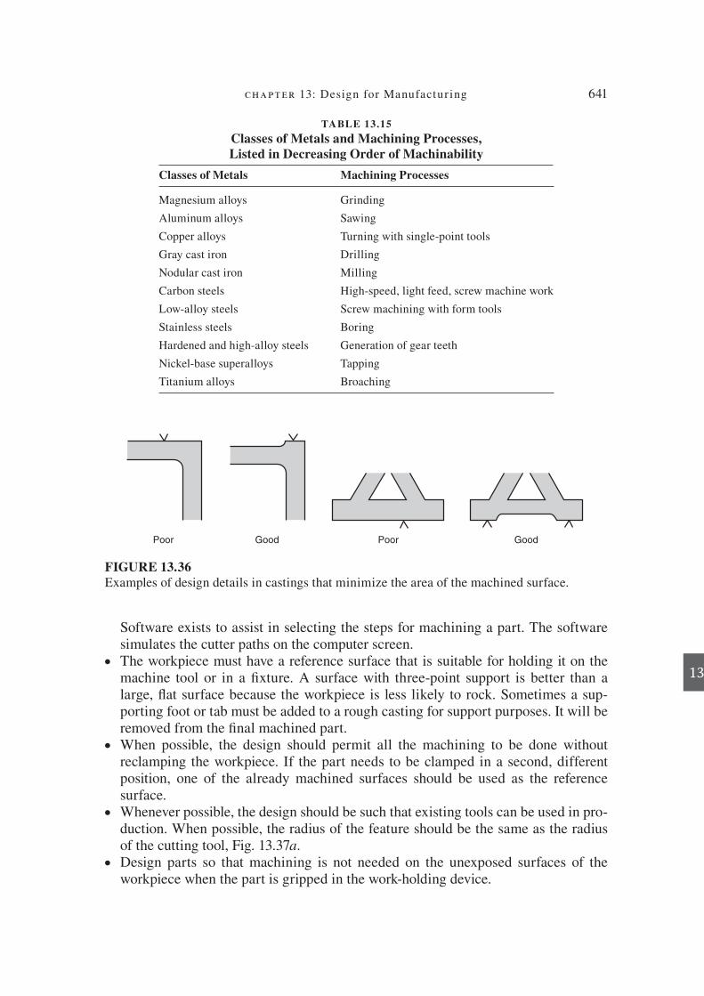
chapter 13: Design for Manufactur ing 641
13
Software exists to assist in selecting the steps for machining a part. The software simulates the cutter paths on the computer screen.
The workpiece must have a reference surface that is suitable for holding it on the machine tool or in a F xture. A surface with three-point support is better than a large, C at surface because the workpiece is less likely to rock. Sometimes a sup-porting foot or tab must be added to a rough casting for support purposes. It will be removed from the F nal machined part.
When possible, the design should permit all the machining to be done without reclamping the workpiece. If the part needs to be clamped in a second, different position, one of the already machined surfaces should be used as the reference surface.
Whenever possible, the design should be such that existing tools can be used in pro-duction. When possible, the radius of the feature should be the same as the radius of the cutting tool, Fig. 13.37 a .
Design parts so that machining is not needed on the unexposed surfaces of the workpiece when the part is gripped in the work-holding device.
●
●
●
●
TABLE 13.15
Classes of Metals and Machining Processes,
Listed in Decreasing Order of Machinability
Classes of Metals Machining Processes
Magnesium alloys Grinding
Aluminum alloys Sawing
Copper alloys Turning with single-point tools
Gray cast iron Drilling
Nodular cast iron Milling
Carbon steels High-speed, light feed, screw machine work
Low-alloy steels Screw machining with form tools
Stainless steels Boring
Hardened and high-alloy steels Generation of gear teeth
Nickel-base superalloys Tapping
Titanium alloys Broaching
FIGURE 13.36
Examples of design details in castings that minimize the area of the machined surface.
GoodPoorGoodPoor
die37039_ch13.indd 641 2/25/08 7:00:05 PM
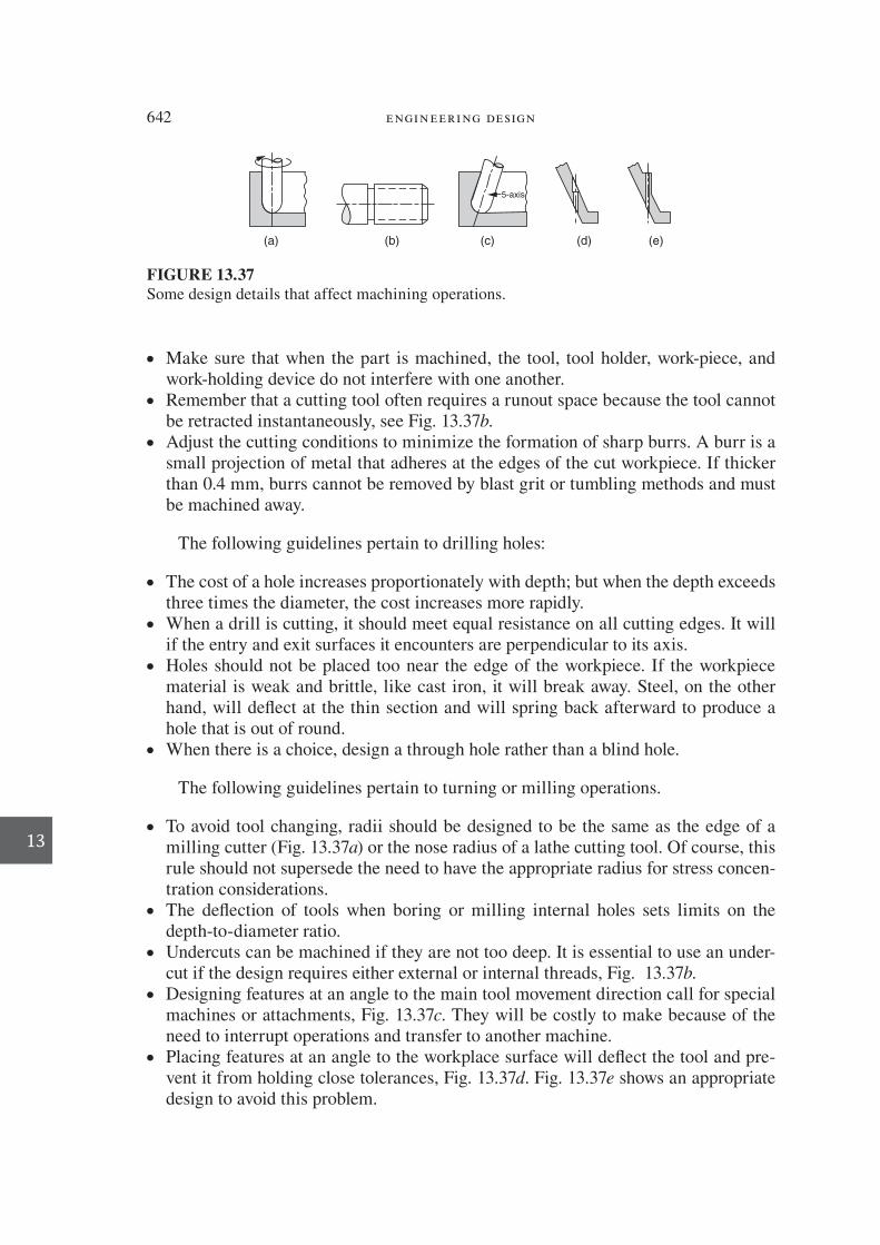
642 engineering design
13
Make sure that when the part is machined, the tool, tool holder, work-piece, and work-holding device do not interfere with one another.
Remember that a cutting tool often requires a runout space because the tool cannot be retracted instantaneously, see Fig. 13.37 b .
Adjust the cutting conditions to minimize the formation of sharp burrs. A burr is a small projection of metal that adheres at the edges of the cut workpiece. If thicker than 0.4 mm, burrs cannot be removed by blast grit or tumbling methods and must be machined away.
The following guidelines pertain to drilling holes:
The cost of a hole increases proportionately with depth; but when the depth exceeds three times the diameter, the cost increases more rapidly.
When a drill is cutting, it should meet equal resistance on all cutting edges. It will if the entry and exit surfaces it encounters are perpendicular to its axis.
Holes should not be placed too near the edge of the workpiece. If the workpiece material is weak and brittle, like cast iron, it will break away. Steel, on the other hand, will deC ect at the thin section and will spring back afterward to produce a hole that is out of round.
When there is a choice, design a through hole rather than a blind hole.
The following guidelines pertain to turning or milling operations.
To avoid tool changing, radii should be designed to be the same as the edge of a milling cutter (Fig. 13.37 a ) or the nose radius of a lathe cutting tool. Of course, this rule should not supersede the need to have the appropriate radius for stress concen-tration considerations.
The deC ection of tools when boring or milling internal holes sets limits on the depth-to-diameter ratio.
Undercuts can be machined if they are not too deep. It is essential to use an under-cut if the design requires either external or internal threads, Fig. 13.37 b .
Designing features at an angle to the main tool movement direction call for special machines or attachments, Fig. 13.37 c . They will be costly to make because of the need to interrupt operations and transfer to another machine.
Placing features at an angle to the workplace surface will deC ect the tool and pre-vent it from holding close tolerances, Fig. 13.37 d . Fig. 13.37 e shows an appropriate design to avoid this problem.
●
●
●
●
●
●
●
●
●
●
●
●
FIGURE 13.37
Some design details that affect machining operations.
(a) (b) (c) (d) (e)
5-axis
die37039_ch13.indd 642 2/25/08 7:00:06 PM

chapter 13: Design for Manufactur ing 643
13
13.15 DESIGN OF WELDING
Welding is the most prominent process for joining large components into complex as-semblies or structures. It is an important area of the wider topic of joining parts into assemblies.
13.15.1 Joining Processes
Technology has created a myriad of joining processes, Fig. 13.38. They can be con-veniently divided into permanent and nonpermanent joints. Nonpermanent joints are used when the assembly must be taken apart for maintenance, repair, or recycling.
Bolts and screws 59 and snap F ts 60 (especially in plastic parts) are most common. Other nonpermanent joining methods are shrink and press F ts, snap rings, pins, and various types of mechanical quick-release mechanisms like clamps and clips.
Permanent mechanical joining methods include riveting, stitching, and stapling of thin materials, and seams produced in sheet metal by making tight bends. Sometimes a sealer such as polymer or solder is used to make the seam impermeable.
The majority of processes for making permanent joints involve melting, either the melting (fusion) of two metals at a joint (welding) or the addition of a molten material at a temperature where the metals at the joint have not melted (brazing. soldering, and adhesive bonding).
An extensive PRIMA selection matrix and data sheets have been developed for joining processes. 61
13.15.2 Welding Processes
Brief descriptions of the most common welding processes 62 follow, starting with the left side of Fig. 13.38.
Solid-State Welding
In solid-state welding, welding is carried out without melting either of the mate-rials to be joined. The oldest welding process is the solid-state method called forge
welding . It is the technique used by the blacksmith in which two pieces of steel or iron are heated and forged together under point contact. Slag and oxides are squeezed out, and interatomic bonding of the metal results. In the modern version of forge welding,
59. The design of bolts and screws is typically covered in machine design texts; see R. G . Budynas and J. K . Nisbet Shigley’s Mechanical Engineering Design, 8 th ed., Chap. 8, McGraw-Hill, New York , 2008 . 60. P. R . Bonenberger , The First Snap-Fit Handbook, 2d ed., Hanser Gardner Publications, Cincinnati, OH , 2005 . 61. K.G . Swift and J. D . Booker, Process Selection, 2d ed., pp. 31–34 and pp. 190–239 , Butterworth-Heinemann, Oxford, UK , 2003 . 62. ASM Handbook, Vol. 6, Welding, Brazing, and Soldering, ASM International, Materials Park, OH , 1993 .
die37039_ch13.indd 643 2/25/08 7:00:06 PM

644 engineering design
13
steel pipe is produced by forming sheet into a cylinder and welding the edges together by forge-seam welding in which either the sheet is pulled through a conical die or the hot strip is passed between shaped rolls.
As the name implies, cold-welding processes are carried out at room temperature without any external heating of the metal. The surfaces must be very clean, and the local pressure must be high enough to produce substantial cold-working. The harmful effect of interface F lms is minimized when there is considerable relative movement of the surfaces to be joined. The movement is achieved by passing the metal through a rolling mill or subjecting the interface to tangential ultrasonic vibration. In explosive bonding there is very high pressure and extensive vorticity at the interfaces. Diffu-sion bonding takes place at a temperature high enough for diffusion to occur readily across the bond zone. Hot roll bonding is a combination of diffusion bonding and roll bonding.
Friction welding (inertia welding) utilizes the frictional heat generated when two bodies slide over each other. In the usual way of doing friction welding, one part is held F xed and the other part (usually a shaft or cylinder) is rotated rapidly and, at the
FIGURE 13.38
ClassiF cation of joining processes.
Joining processes
Nonpermanent
Mechanical
Cold welding Diffusion
Nonconsumable electrode Consumable electrode Consumable workpiece
Hot welding Friction Electron beam
Laser beam
Brazing
Soldering
Adhesive
bonding
Solid-state
Electric arc High-energy- ThermalResistance
welding welding weldingbeam welding
Liquid-state (fusion) Liquid-solid
Permanent
Screw
Snap
Shrink
Rivet
Stitch
Staple
Lap-seam
Pressure
Roll
Explosion
Ultrasonic
Pressure Forge
Roll
Gas-W arc (TIG)
Plasma arc
Carbon arc
Gas-metal arc (MIG)
Shielded metal arc
Flux-cored
Submerged arc
Electroslag
Electrogas
Stud
Capacitor discharge
Percussion
welding
Spot
Projection
Seam
Flash-upset
High-frequency
HF induction
Gas
Thermite
die37039_ch13.indd 644 2/25/08 7:00:06 PM

chapter 13: Design for Manufactur ing 645
13
same time, forced axially against the stationary part. The friction quickly heats the abutting surfaces and, as soon as the proper temperature is reached, the rotation is stopped and the pressure is maintained until the weld is complete. The impurities are squeezed out into a C ash, but essentially no melting takes place. The heated zone is very narrow, and therefore dissimilar metals are easily joined.
Liquid-State Welding (Fusion Welding)
In the majority of welding processes a bond between the two materials is produced by melting, usually with the addition of a F ller metal. In welding, the workpiece mate-rials and the F ller material in the joint have similar compositions and melting points. By contrast, in soldering and brazing, the F ller material has a much different compo-sition that is selected to have a lower melting point than the workpiece materials.
Resistance welding utilizes the heat generated at the interface between two metal parts when a high current is passed through the parts. Spot welding is used exten-sively to join metal sheets by melting them at discrete points (spots) under pressure from the electrodes. Rather than produce a series of spots, an electrode in the form of a roller often is used to produce a seam weld. If the part to be welded contains small embossed projections, they are easily softened under the electrode and pushed back to produce the weld nugget.
Heat for welding comes from chemical sources or high-energy beams. Gas weld-ing, especially the reaction between oxygen and acetylene to produce an intense C ame, has been used for many years. Thermite welding uses the reaction between Fe 2 O 3 and Al, which produces Fe and an intense heat. The process is used to weld heavy sections such as rails. Energy from a laser beam is used to produce welds in sheet metal. Its ad-vantage over an electron beam is that a vacuum is not required. Each form of energy is limited in power, but it can be carefully controlled. Laser beam and electron beam welding lend themselves to welding thin gauges of hardened or high- temperature materials.
The thermal energy produced from an electric arc has been utilized extensively in welding. Most electric arc welding is done with an arc struck between a consumable electrode (the F ller or weld rod) and the workpiece. A coating is applied to the outside surface of the metal electrode to provide a protective atmosphere around the weld pool. The electrode coating also acts as a C ux to remove impurities from the molten metal and as an ionizing agent to help stabilize the arc. This is the commonly used shielded metal arc process . Since the electrode coating is brittle, only straight stick electrodes can be used. That restricts the process to a slow hand operation. If the C ux coating is placed inside a long tube, the electrode can be coiled, and then the shielded arc process can be made continuous and automatic. In the submerged arc process the consumable electrode is a bare F ller wire, and the C ux is supplied from a separate hopper in a thick layer that covers the arc and the weld pool. In the electroslag process the electrode wire is fed into a pool of molten slag that sits on top of the molten weld pool. Metal transfer is from the electrode to the weld pool through the molten slag. This process is used for welding thick plates and can be automated. In the gas metal
arc (MIG) process the consumable metal electrode is shielded by an inert gas such as argon or helium. Because there is no C ux coating, there is no need to remove the slag deposit from the weld bead after each pass.
die37039_ch13.indd 645 2/25/08 7:00:07 PM

646 engineering design
13
In nonconsumable electrode welding an inert tungsten electrode is used. Depend-ing on the weld design, a F ller rod may be required. In gas tungsten arc welding (TIG welding), argon or helium is used. The process produces high-quality welds in almost any material, especially in thinner-gauge sheet. The two most common welding meth-ods are the metal arc process for welding large structures like ships, pipelines, and bridges, and TIG welding for smaller machine structures and thin sheet.
Liquid-Solid-State Welding
In this class of welding processes the temperature generated is not high enough to melt the metals to be joined. Brazing uses low-melting-point alloys of copper, gold, or silver to bond steel, cast iron, and aluminum alloys. Low-melting-point solders are used in joining copper and aluminum wires and in joining electronic components in printed circuit boards. To create a good bond in either brazing or soldering, a C ux must be added to clean oxide F lms from the metal surfaces, prevent further oxida-tion during heating, and assist in the wetting of the metal surfaces. The materials used in brazing and soldering are much weaker than the base metals they join. They can only create a strong bond if there is excellent bonding of the F ller metal with the base metal, and if the joint thickness is the proper amount. To achieve good bonding, the base metal must be free of oxides and organics, and the F ller metal must com-pletely wet the base metal surfaces. Since F ller metal is inherently weaker than the base metal, it gets its strength from the constraint imposed by the thicker and stronger base metal plates. If the F ller layer is too thick, the F ller metal properties will control and the joint strength will be weak. If the F ller layer is too thin, then there may be dif-F culty drawing in the liquid by capillary action. Typically the optimum joint thickness is about 5 to 10 mm.
Adhesive bonding uses a liquid polymer as the F ller material. It can be used to join plastics, metals, or ceramics in applications where the stresses are rather low. Adhesive bonding depends solely on adhesion forces to provide the bond. Thus, the surfaces must be very clean, although some surface roughness can be advantageous to increase the surface area. The adhesive must completely wet the surface to give complete coverage, and as with soldering and brazing, the joint gap must be small and well controlled. The technology of adhesive bonding has advanced rapidly and today is used to bond surfaces in aircraft and automotive products.
13.15.3 Welding Design
To design a weldment, consideration must be given to the selection of materials, the joint design, the selection of the welding process, and the stresses that must be re-sisted by the design. The welding process subjects the workpiece at the joint to a tem-perature that exceeds the melting point of the material. Heat is applied locally and rapidly to create a miniature casting in the weld pool. Often successive weld passes are laid down. The base metal next to the weld bead, the heat-affected zone (HAZ), is subjected to rapid heating and cooling, so the original microstructure and prop-erties of the base metal are changed, Fig. 13.39. The F gure shows coarse columnar grains characteristic of a casting in the weld joint. Into the base metal the elongated
die37039_ch13.indd 646 2/25/08 7:00:07 PM

chapter 13: Design for Manufactur ing 647
13
cold-worked grains have recrystallized and formed a large grain size near the original joint boundary, falling off in grain size throughout the region of the HAZ because of the difference in temperature and time that they have seen. Considerable opportunity for defects exists unless the welding process is properly carried out.
Material Behavior and Selection
Since fusion welding is a melting process, controls appropriate to producing qual-ity castings must be applied. Reactions with the atmosphere are prevented by sealing off the molten pool with an inert gas or a slag or by carrying out the welding in a vac-uum chamber. The surfaces of the weld joint should be cleaned of scale or grease be-fore welding is undertaken. The thermal expansion of the weld structure upon heating, followed by solidiF cation shrinkage, can lead to high internal tensile stresses that can produce cracking and/or distortion. Rapid cooling of alloy steels in welding can result in brittle martensite formation and consequent crack problems: see Fig. 13.43a. As a result, it is common to limit welding to carbon steels with less than 0.3 percent car-bon or to alloy steels in which the carbon equivalent 63 is less than 0.3 percent carbon. When steels with 0.3 to 0.6 percent carbon must be used because their high strength is required, welding without martensite cracking can be performed if the weld joint is preheated before welding and postheated after the weld bead has been deposited. These thermal treatments decrease the rate of cooling of the weld and heat-affected zone, and they reduce the likelihood of martensite formation.
Material selection for welding involves choosing a material with high weldability. Weldability, like machinability, is a complex technological property that combines many more basic properties. The melting point of the material, together with the spe-ciF c heat and latent heat of fusion, will determine the heat input necessary to pro-duce fusion. A high thermal conductivity allows the heat to dissipate and therefore requires a higher rate of heat input. Metals with higher thermal conductivity result in more rapid cooling and more problems with weld cracking. Greater distortion results from a high thermal expansion, with higher residual stresses and greater danger of weld cracking. There is no absolute rating of weldability of metals because different
FIGURE 13.39
Sketch showing the grain structure in a section through an electric arc weld in two rolled metal plates.
Original
workpiece
edge
Melt
boundary Coarse Recrystallized
grains
Original
cold-worked
grains
HAZ
Fine
63. C CMn
6
Cr + Mo + V
5
Ni + Cueq
= + + +15
die37039_ch13.indd 647 2/25/08 7:00:07 PM
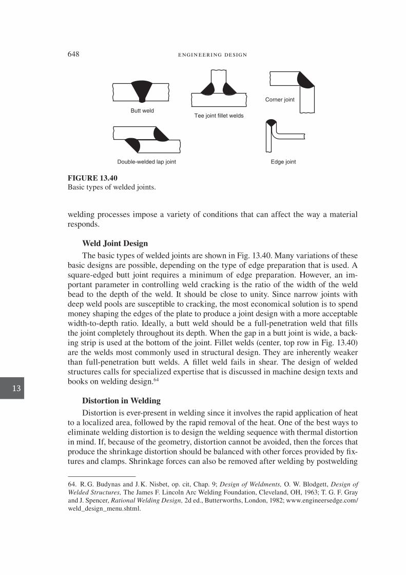
648 engineering design
13
welding processes impose a variety of conditions that can affect the way a material responds.
Weld Joint Design
The basic types of welded joints are shown in Fig. 13.40. Many variations of these basic designs are possible, depending on the type of edge preparation that is used. A square-edged butt joint requires a minimum of edge preparation. However, an im-portant parameter in controlling weld cracking is the ratio of the width of the weld bead to the depth of the weld. It should be close to unity. Since narrow joints with deep weld pools are susceptible to cracking, the most economical solution is to spend money shaping the edges of the plate to produce a joint design with a more acceptable width-to-depth ratio. Ideally, a butt weld should be a full-penetration weld that F lls the joint completely throughout its depth. When the gap in a butt joint is wide, a back-ing strip is used at the bottom of the joint. Fillet welds (center, top row in Fig. 13.40) are the welds most commonly used in structural design. They are inherently weaker than full-penetration butt welds. A F llet weld fails in shear. The design of welded structures calls for specialized expertise that is discussed in machine design texts and books on welding design. 64
Distortion in Welding
Distortion is ever-present in welding since it involves the rapid application of heat to a localized area, followed by the rapid removal of the heat. One of the best ways to eliminate welding distortion is to design the welding sequence with thermal distortion in mind. If, because of the geometry, distortion cannot be avoided, then the forces that produce the shrinkage distortion should be balanced with other forces provided by F x-tures and clamps. Shrinkage forces can also be removed after welding by postwelding
FIGURE 13.40
Basic types of welded joints.
Double-welded lap joint
Butt weldTee joint fillet welds
Corner joint
Edge joint
64. R. G . Budynas and J. K . Nisbet , op. cit, Chap. 9; Design of Weldments, O. W . Blodgett , Design of
Welded Structures, The James F. Lincoln Arc Welding Foundation, Cleveland, OH , 1963 ; T. G. F . Gray and J . Spencer , Rational Welding Design, 2d ed., Butterworths, London , 1982 ; www.engineersedge.com/weld_design_menu.shtml.
die37039_ch13.indd 648 2/25/08 7:00:08 PM

chapter 13: Design for Manufactur ing 649
13
annealing and stress-relief operations. Distortion can be minimized by specifying in the design only the amount of weld metal that is absolutely required. Overwelding adds not only to the shrinkage forces but also to the costs.
DFM Guidelines for Welding
The following are some general considerations applicable in designing a welded part.
Welded designs should reC ect the C exibility and economy inherent in the welding process. Do not copy designs based on casting or forging.
In the design of welded joints, provide for straight force C owlines. Avoid the use of welded straps, laps, and stiffeners except as required for strength. Use the mini-mum number of welds.
Weld together parts of equal thickness whenever possible. Locate the welds at areas in the design where stresses and/or deC ections are least critical.
Carefully consider the sequence with which parts should be welded together and include that information as part of the engineering drawing.
Make sure that the welder or welding machine (for automatic welding) has unob-structed access to the joint so that a quality weld can be produced. Whenever pos-sible, the design should provide for welding in the C at or horizontal position, not overhead.
13.15.4 Cost of Joining
We can adapt the cost of manufacture model presented in Sec.13.4.6 to cover the cost of joining parts. This supplements the method of estimating assembly costs that was outlined in Sec. 13.10.1. The cost of joining per unit assembly or subassembly, C join , is given by 65
C C C tC
n
C
LtC t
L process
t o
join com
wo
OH= + × + +
pprocess
setup
batch
t
n+
all joinnts
n
∑ (13.15)
where C com is the cost of consumable materials such as weld rod, C ux, adhesives, or fasteners C t is the cost of dedicated jigs and F xtures n is the number of joints to be made in the entire production run t process is the time to create a single weld or adhesive joint, or to insert and torque a single fastener
The other symbols in Eq. (13.15) have the same meaning as given in Sec. 13.3.
●
●
●
●
●
●
65. A. M. K . Esawi and M. F . Ashby , Materials and Design, Vol. 24, pp. 605–16 , 2003 .
die37039_ch13.indd 649 2/25/08 7:00:08 PM

650 engineering design
13
13.16 RESIDUAL STRESSES IN DESIGN
Residual stresses are the system of stresses that can exist in a part when the part is free from external forces. They are sometimes referred to as internal stresses or locked-in stresses. 66 They arise from nonuniform plastic deformation of a solid, chieC y as a re-sult of inhomogeneous changes in volume or shape that occur during manufacturing processes.
13.16.1 Origin of Residual Stresses
Residual stresses are developed due to nonuniform deformation. To understand how, consider an assembly that is made by joining a core and a tight-F tting tube 67 (Fig. 13.41 a ). Both components are made from the same material and have equal cross-sectional areas. The core was longer than the tube, so before they were joined by welding the core was compressed by a F xture to the same length as the tube, (Fig. 13.41 b ). After making the weld, the F xture compressing the core was removed and the assembly assumed a new length somewhere between the original lengths of
FIGURE 13.41
Example of the formation of residual stresses due to inhomogeneous deformation.
Atube
l tub
e
l cu
be
Acube
(a) (b)
(1) Tensile
(2) Compressive
(c)
66. W. B . Young, ed. , Residual Stresses in Design, Process and Materials Selection, ASM Interna-tional, Materials Park, OH , 1987 ; U . Chandra, “Control of Residual Stresses,” ASM Handbook, Vol. 20, pp. 811–19 , ASM International, Materials Park, OH , 1997 . 67. J. A . Schey , Introduction to Manufacturing Processes, 3d ed., pp. 105–6, McGraw-Hill, New York , 2000 .
die37039_ch13.indd 650 2/25/08 7:00:08 PM

chapter 13: Design for Manufactur ing 651
13
the two components. Now the core wants to expand to its original length, and the tube wants to return to its original length, but they are now joined as a single assembly and the individual components cannot move. The tube has extended relative to its original length so it is subjected to tensile residual stresses. The core has been compressed relative to its original length so it is subjected to compressive residual stresses. Even though there is no external load on the assembly it has a tensile stress at its surface and a compressive stress in its core (Fig. 13.41 c ). Because the areas of tube and core are equal, the stresses are equal and uniform in each region. The residual stress system existing in the assembly after reaching its F nal state (c) must be in static equilibrium. Thus, the total force acting on any plane through the body and the total moment of forces on any plane must be zero. For the longitudinal stress pattern in Fig. 13.41 this means that the area subjected to compressive residual stresses must balance the area subjected to tensile residual stresses.
The situation regarding residual stress generation is not quite so simple as is pic-tured in Fig. 13.41. Often residual stresses in deformation processes arise from having regions of heavy plastic deformation contiguous to regions of light deformation. The boundaries between these regions are not as simple nor are the volumes of the regions the same as in the previous example, but the results are the same. Regions of the part that have been required to deform in tension will upon unloading develop compres-sive residual stresses, and vice versa. In some cases the residual stresses acting in the three principal directions need to be known. The state of residual stress at any point is a combined stress derived from the residual stresses in the three principal directions. Frequently, because of symmetry, only the residual stress in one direction need be considered. A complete determination of the state of residual stress in three dimen-sions is a considerable undertaking.
Residual stresses cannot exceed the value of the yield stress of the material. A stress in excess of that value, with no external force to oppose it, will relieve itself by plastic deformation until it reaches the value of the yield stress. Residual stress and stresses from applied forces add algebraically, so long as their sum does not exceed the yield stress of the material. For example, if the maximum applied stress due to ap-plied loads is 60,000 psi tension and the part already contains a tensile residual stress of 40,000 psi, the total stress at the critically stressed region is 100,000 psi. However if the residual stress is a compressive 40,000 psi produced by shot peening, then the actual stress is 20,000 psi.
In Fig. 13.41, if the weld holding together the two components was machined away, each component would be free to assume its original length. The assembly would undergo distortion from its intended shape. The same thing happens in parts with more complex residual stress distributions. If they are machined, removing ma-terial alters the residual stress distribution and the new balance of forces may cause distortion of the part.
Any process, whether mechanical, thermal, or chemical, that produces a perma-nent nonuniform change in shape or volume creates a residual stress pattern. Prac-tically, all cold-working operations develop residual stresses because of nonuniform plastic C ow. In surface-working operations, such as shot peening, surface rolling, or polishing, the penetration of the deformation is very shallow. The distended surface layer is held in compression by the less-worked interior.
die37039_ch13.indd 651 2/25/08 7:00:09 PM

652 engineering design
13
A surface compressive residual stress pattern is highly effective in reducing the incidence of fatigue failure.
Residual stresses arising from thermal processes may be classiF ed as those due to a thermal gradient alone or to a thermal gradient in conjunction with a phase trans-formation, as in heat-treating steel. These stresses arise most frequently in quenching during heat treatment, or in heating and cooling experienced in casting and welding.
The control of residual stresses starts with understanding the fundamental source of the stress and identifying the parameters in the manufacturing process that inC u-ence the stress. Then, experiments are performed in varying the process parameters to produce the desired level of stress. FEA modeling has been used effectively in pre-dicting how residual stresses can be reduced. 68
13.16.2 Residual Stress Created by Quenching
The case of greatest practical interest involves the residual stresses developed dur-ing the quenching of steel for hardening. The residual stress pattern created is due to thermal volume changes plus volume changes resulting from the transformation of austenite to martensite. The simpler situation, in which the stresses are due only to thermal volume changes, will be considered F rst. This is the situation encountered in the quenching of a metal that does not undergo a phase change on cooling, like cop-per. This condition is also present when steel is quenched from a tempering tempera-ture below the A 1 critical temperature.
The distribution of residual stress over the diameter of a quenched bar in the lon-gitudinal, tangential, and radial directions is shown in Fig. 13.42 a for the most com-mon situation of a metal that contracts on cooling. Figure 13.42 c shows that the oppo-site residual stress distribution is obtained if the metal expands on cooling (this occurs for only a few materials). The sequence of events producing the stress pattern shown in Fig. 13.42a is as follows: The relatively cool surface of the bar tends to contract into a ring that is both shorter and smaller in diameter than it was originally. This tends to extrude the hotter, more plastic center into a cylinder that is longer and thinner than it was originally. If the inner core were free to change shape independently of the outer region of the bar, it would change dimensions to a shorter and thinner cylinder on cooling. Mechanics of materials principles require that continuity must be maintained throughout the bar. Thus, the outer ring is drawn in (compressed) in the longitudinal, tangential, and radial directions at the same time the inner core is extended in the same directions. The stress pattern shown in Fig. 13.42 a results.
The magnitude of the residual stresses produced by quenching depends on the stress-strain relationship for the metal and the degree of strain mismatch produced by the quenching operation. For a given strain mismatch, the higher the elastic modulus of the metal the higher the residual stress. Further, since the residual stress cannot ex-ceed the yield stress, the higher the yield stress the higher the possible residual stress. The yield stress–temperature curve for the metal also is important. If the yield stress
68. U . Chandra , op. cit.
die37039_ch13.indd 652 2/25/08 7:00:09 PM

chapter 13: Design for Manufactur ing 653
13
decreases rapidly with increasing temperature, the strain mismatch will be small at high temperatures because the metal can accommodate to thermally produced volume changes by plastic C ow. Metals that have a high yield strength at elevated tempera-tures, like nickel base superalloys, will develop strain mismatches in quenching, lead-ing to high residual stresses.
The following physical properties will lead to high mismatch strains on quenching:
Low thermal conductivity, k High speciF c heat, c High density, r High coefF cient of thermal expansion, a
The F rst three factors can be combined into the thermal diffusivity D 5 k /r c . Low values of thermal diffusivity lead to high strain mismatch. Other process conditions that produce an increase in the temperature difference between the surface and cen-ter of the bar promote high quenching stresses. They are (1) a large diameter of the cylinder, (2) a large temperature difference between the initial temperature and the temperature of the quenching bath, and (3) rapid heat transfer at the metal-liquid interface.
In the quenching of steels, austenite (the high-temperature form of steel) begins to transform to martensite whenever the local temperature of the bar reaches the M s temperature. Since an increase in volume accompanies the phase transformation,
●
●
●
●
L
R
T
Longitudinal
L = longitudinal
T = tangential
R = radial
+
–
Longitudinal
Tangential Tangential
Radial Radial
(a) (c)(b)
FIGURE 13.42
Residual stress patterns found in quenched bars and due to thermal strains (schematic). (a) For metal that contracts on cooling; (b) orientation of directions; (c) for metal that expands on cooling.
die37039_ch13.indd 653 2/25/08 7:00:09 PM

654 engineering design
13
the metal expands as the martensite reaction proceeds on cooling from the M s to M f temperature. 69 This produces a residual stress distribution of the type shown in Fig. 13.42 c . The residual stress distribution in a quenched steel bar is the resultant of the competing processes of thermal contraction and volume expansion due to martensite formation. The resulting stress pattern depends upon the transformation characteris-tics of the steel, as determined chieC y by composition and hardenability, 70 the heat-transfer characteristics of the system, and the severity of the quench.
Figure 13.43 illustrates some of the possible residual stress patterns that can be produced by quenching steel bars. On the left side of the F gure is an isothermal trans-formation diagram for the decomposition of austenite. To form martensite the bar must cool fast enough to avoid entering the area where soft pearlite forms. The cool-ing rates of the outside, midradius, and center of the bar are indicated on the diagram by the curves marked o , m , and c . In Fig. 13.43 a the quenching rate is rapid enough to convert the entire bar to martensite. By the time the center of the bar reaches the M s temperature, the transformation has been essentially completed at the surface. The surface layers try to contract against the expanding central core, and the result is ten-sile residual stresses at the surface and compressive stresses at the center of the bar (Fig. 13.43 b ). However, if the bar diameter is rather small and the bar has been dras-tically quenched in brine so that the surface and center transform at about the same time, the surface will arrive at room temperature with compressive residual stresses. If the bar is slack-quenched so that the outside transforms to martensite while the middle and center transform to pearlite (Fig. 13.43 c ), there is little restraint offered by the hot, soft core during the time when martensite is forming on the surface, and the core readily accommodates to the expansion of the outer layers. The middle and center pearlite regions then contract on cooling in the usual manner and produce a re-sidual stress pattern consisting of compression on the surface and tension at the center (Fig. 13.43 d ).
13.16.3 Other Issues Regarding Residual Stresses
The two previous sections were concerned with residual stresses produced by inhomo-geneous plastic deformation due to mechanical forces or constraints, due to thermal expansion, or due to volume changes as a result of solid-state transformations. In this section we brieC y discuss several additional important issues about residual stresses.
The residual stresses in castings are often modeled by a quenched cylinder. How-ever, the situation in castings is made more complicated by the fact that the mold acts as a mechanical restraint to the shrinking casting. Moreover, the casting de-sign may produce greatly different cooling rates at different locations that are due to variations in section size and the introduction of chills. Chills are metal plates added to a sand mold to produce an artiF cially rapid cooling rate.
●
69 . M s and M f are the temperatures at which martensite starts to form and F nishes forming, respectively, on quenching. 70 . Hardenability is an engineering measurement of the depth of hardening in a steel as a result of quenching into a speciF c medium.
die37039_ch13.indd 654 2/25/08 7:00:09 PM

chapter 13: Design for Manufactur ing 655
13
Appreciable residual stresses are developed in welding, even in the absence of a phase transformation. As the weld metal and heat-affected zone shrink on cooling, they are restricted by the cooler surrounding plate. The result is that the weld re-gion contains tensile residual stresses, which are balanced by compressive stresses in a region of the plate outside of the heat-affected zone. Because thermal gradients tend to be high in welding, the residual stress gradients also tend to be high. Re-sidual stresses in welds are often involved in weld cracking.
Chemical processes such as oxidation, corrosion, and electroplating can generate large surface residual stresses if the new surface material retains coherency with the underlying metal surface. Other surface chemical treatments such as carburiz-ing and nitriding cause local volume changes by the diffusion of an atomic species into the surface, and this can result in residual stresses.
●
●
FIGURE 13.43
Transformation characteristics of a steel (a and c), and resulting residual stress distributions (b and d).
Austenite
Pearlite
Martensite
0
0
0
+
–
log time
(a) (b)
Te
mp
era
ture
o m
T
R
L
c
Ms
Austenite
Pearlite
Martensite
0
0
0
+
–
log time
(c) (d)
Te
mp
era
ture
o
m
T
R
L
c
Ms
die37039_ch13.indd 655 2/25/08 7:00:10 PM
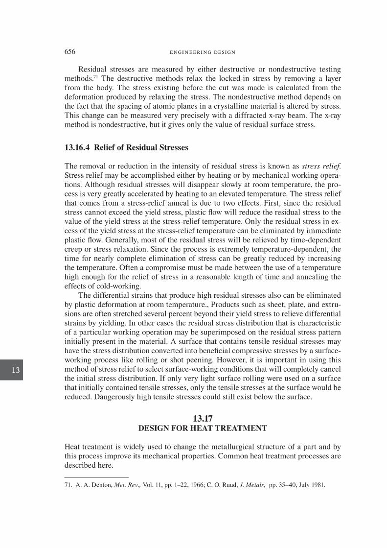
656 engineering design
13
Residual stresses are measured by either destructive or nondestructive testing methods. 71 The destructive methods relax the locked-in stress by removing a layer from the body. The stress existing before the cut was made is calculated from the deformation produced by relaxing the stress. The nondestructive method depends on the fact that the spacing of atomic planes in a crystalline material is altered by stress. This change can be measured very precisely with a diffracted x-ray beam. The x-ray method is nondestructive, but it gives only the value of residual surface stress.
13.16.4 Relief of Residual Stresses
The removal or reduction in the intensity of residual stress is known as stress relief . Stress relief may be accomplished either by heating or by mechanical working opera-tions. Although residual stresses will disappear slowly at room temperature, the pro-cess is very greatly accelerated by heating to an elevated temperature. The stress relief that comes from a stress-relief anneal is due to two effects. First, since the residual stress cannot exceed the yield stress, plastic C ow will reduce the residual stress to the value of the yield stress at the stress-relief temperature. Only the residual stress in ex-cess of the yield stress at the stress-relief temperature can be eliminated by immediate plastic C ow. Generally, most of the residual stress will be relieved by time-dependent creep or stress relaxation. Since the process is extremely temperature-dependent, the time for nearly complete elimination of stress can be greatly reduced by increasing the temperature. Often a compromise must be made between the use of a temperature high enough for the relief of stress in a reasonable length of time and annealing the effects of cold-working.
The differential strains that produce high residual stresses also can be eliminated by plastic deformation at room temperature., Products such as sheet, plate, and extru-sions are often stretched several percent beyond their yield stress to relieve differential strains by yielding. In other cases the residual stress distribution that is characteristic of a particular working operation may be superimposed on the residual stress pattern initially present in the material. A surface that contains tensile residual stresses may have the stress distribution converted into beneF cial compressive stresses by a surface-working process like rolling or shot peening. However, it is important in using this method of stress relief to select surface-working conditions that will completely cancel the initial stress distribution. If only very light surface rolling were used on a surface that initially contained tensile stresses, only the tensile stresses at the surface would be reduced. Dangerously high tensile stresses could still exist below the surface.
13.17 DESIGN FOR HEAT TREATMENT
Heat treatment is widely used to change the metallurgical structure of a part and by this process improve its mechanical properties. Common heat treatment processes are described here.
71. A. A . Denton , Met. Rev., Vol. 11, pp. 1–22, 1966 ; C. O . Ruud, J. Metals, pp. 35–40 , July 1981 .
die37039_ch13.indd 656 2/25/08 7:00:10 PM

chapter 13: Design for Manufactur ing 657
13
Annealing is heating a metal or alloy to an elevated temperature, holding at tem-perature for enough time to allow a desired metallurgical change to occur, and then cooling slowly to room temperature. It is used to relieve residual stresses, to ho-mogenize a cast structure so that chemical segregation is minimized, or to remove the hardening effects of cold working and through the generation of new strain-free grains (recrystallization) create a structure that has adequate ductility to allow ad-ditional working.
Quenching of steels to produce hard but brittle martensite has been described in the previous section. Quenching must be followed by heating below the transforma-tion temperature ( A 1 ) to temper the martensite into a precipitation of F ne carbides. Quenched and tempered (Q&T) steels are the engineering materials with the best combination of readily achievable strength and toughness.
Many nonferrous alloys, especially aluminum alloys, are strengthened by F rst heat-ing to solution treatment temperature to put the alloying elements into solid solu-tion, and then cooling rapidly to an aging temperature. The alloy is held (aged) for a sufF cient time to allow the formation of a F ne precipitate that hardens the alloy.
13.17.1 Issues with Heat Treatment
Processing by heat treatment requires energy. It also requires a protective atmosphere or surface coating on the metal to prevent the part from oxidizing or otherwise react-ing with the furnace atmosphere. During long exposure at elevated temperatures, metal parts soften, creep, and eventually sag. Therefore, parts may require special F xtures to support them during heat treatment. Since heat treatment is a secondary processing step, it would be advantageous to eliminate the need whenever possible. Sometimes a part made from a cold-worked sheet or bar can be substituted for a heat-treated part to achieve the needed strength properties. Usually the C exibility and/or superior proper-ties that result from heat treatment make it the preferred choice in manufacturing.
The best combination of high strength and high toughness is produced in a steel by F rst heating within the austenite temperature region (1400 to 1650°F) and then quenching rapidly enough that hard and brittle martensite is formed (see Fig. 13.43). The part is then reheated below the austenite region to allow the martensite to break down (temper) into a F ne precipitation of carbides in a soft ferrite (iron) matrix. Achieving a proper quenched and tempered microstructure depends on cooling fast enough that pearlite or other nonmartensitic phases are not formed. This requires a balance between the heat transfer from the part (as determined chieC y by geometry), the cooling power of the quenching medium (brine, water, oil, or air), and the trans-formation kinetics of the steel (as controlled by the alloy chemistry). These factors are interrelated by the property called hardenability. 72
In heating for austenitization, care should be taken to subject the parts to uniform temperature in the furnace. Long, thin parts are especially prone to distortion from
●
●
●
72. ASM Handbook, Vol. 4, Heat Treating, ASM International, Materials Park, OH , 1991 ; C. A . Siebert , D. V . Doane , and D. H . Breen, The Hardenability of Steels, ASM International, Materials Park, OH , 1977 .
die37039_ch13.indd 657 2/25/08 7:00:10 PM
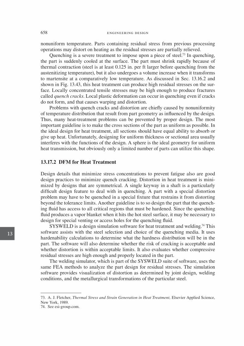
658 engineering design
13
nonuniform temperature. Parts containing residual stress from previous processing operations may distort on heating as the residual stresses are partially relieved.
Quenching is a severe treatment to impose upon a piece of steel. 73 In quenching, the part is suddenly cooled at the surface. The part must shrink rapidly because of thermal contraction (steel is at least 0.125 in. per ft larger before quenching from the austenitizing temperature), but it also undergoes a volume increase when it transforms to martensite at a comparatively low temperature. As discussed in Sec. 13.16.2 and shown in Fig. 13.43, this heat treatment can produce high residual stresses on the sur-face. Locally concentrated tensile stresses may be high enough to produce fractures called quench cracks . Local plastic deformation can occur in quenching even if cracks do not form, and that causes warping and distortion.
Problems with quench cracks and distortion are chieC y caused by nonuniformity of temperature distribution that result from part geometry as inC uenced by the design. Thus, many heat-treatment problems can be prevented by proper design. The most important guideline is to make the cross sections of the part as uniform as possible. In the ideal design for heat treatment, all sections should have equal ability to absorb or give up heat. Unfortunately, designing for uniform thickness or sectional area usually interferes with the functions of the design. A sphere is the ideal geometry for uniform heat transmission, but obviously only a limited number of parts can utilize this shape.
13.17.2 DFM for Heat Treatment
Design details that minimize stress concentrations to prevent fatigue also are good design practices to minimize quench cracking. Distortion in heat treatment is mini-mized by designs that are symmetrical. A single keyway in a shaft is a particularly difF cult design feature to deal with in quenching. A part with a special distortion problem may have to be quenched in a special F xture that restrains it from distorting beyond the tolerance limits. Another guideline is to so design the part that the quench-ing C uid has access to all critical regions that must be hardened. Since the quenching C uid produces a vapor blanket when it hits the hot steel surface, it may be necessary to design for special venting or access holes for the quenching C uid.
SYSWELD is a design simulation software for heat treatment and welding. 74 This software assists with the steel selection and choice of the quenching media. It uses hardenability calculations to determine what the hardness distribution will be in the part. The software will also determine whether the risk of cracking is acceptable and whether distortion is within acceptable limits. It also evaluates whether compressive residual stresses are high enough and properly located in the part.
The welding simulator, which is part of the SYSWELD suite of software, uses the same FEA methods to analyze the part design for residual stresses. The simulation software provides visualization of distortion as determined by joint design, welding conditions, and the metallurgical transformations of the particular steel.
73. A. J . Fletcher , Thermal Stress and Strain Generation in Heat Treatment, Elsevier Applied Science, New York , 1989. 74 . See esi-group.com.
die37039_ch13.indd 658 2/25/08 7:00:11 PM

chapter 13: Design for Manufactur ing 659
13
13.18 DESIGN FOR PLASTICS PROCESSING
The manufacturing processes used with plastics must accommodate to the unique C ow properties of polymers. Compared to metals, the C ow stress of a plastic part is much lower and highly strain rate dependent, the viscosity is much higher than liquid metal, and the formability is much greater. See Sec. 12.6 for a discussion of how the proper-ties of plastics affect their use in design. Plastics divide broadly into (1) thermoplastic polymers (TP) that soften on heating and harden when cooled and can be remelted repeatedly; (2) thermosetting polymers (TS) that set or cross-link upon heating in an irreversible way; and (3) polymer composites that have either a TS or TP matrix rein-forced with F bers of glass or graphite. TP polymers are polymerized in their primary manufacturing step and enter plastics processing as a granule or pellet resin. TS poly-mers are polymerized during the processing step, usually by the addition of a catalyst or simply by the addition of heat.
The plastic manufacturing processes considered in this section are:
Injection molding (mostly TP) Extrusion (TP) Blow molding (TP) Rotational molding (TP) Thermoforming (TP) Compression molding (mostly TS) Casting (mostly TS) Composite processing (mostly TS)
Plastic manufacturing processes excel in producing parts with good surface F nish and F ne detail. 75 By adding dyes and colorants, the part can be given a color that elimi-nates a secondary painting operation. However, the cycle time is usually longer than for metal-working processes. Depending on the plastic process, the cycle time can vary from 10 s to 10 h. Generally plastics manufacturing is the preferred method for producing small- to medium-sized parts for consumer and electronic products where mechanical stresses in parts are not too high.
13.18.1 Injection Molding
Injection molding is a process in which plastic granules are heated and forced under pressure into a die cavity (see Fig. 13.2). It is a fast process (10 to 60 s cycle time) that is economical for production runs in excess of 10,000 parts. It is well suited for
●
●
●
●
●
●
●
●
75. Tool and Manufacturing Engineers Handbook, Vol. 8, Plastic Part Manufacturing, Society of Man-ufacturing Engineers, Dearborn, MI , 1996 ; “Engineering Plastics,” Engineered Materials Handbook Vol. 2, Sec. 3, ASM International, Materials Park, OH , 1988 ; E. A . Muccio , “Design for Plastics Process-ing,” ASM Handbook, Vol. 20, pp. 793–803 , 1997 .
die37039_ch13.indd 659 2/25/08 7:00:11 PM
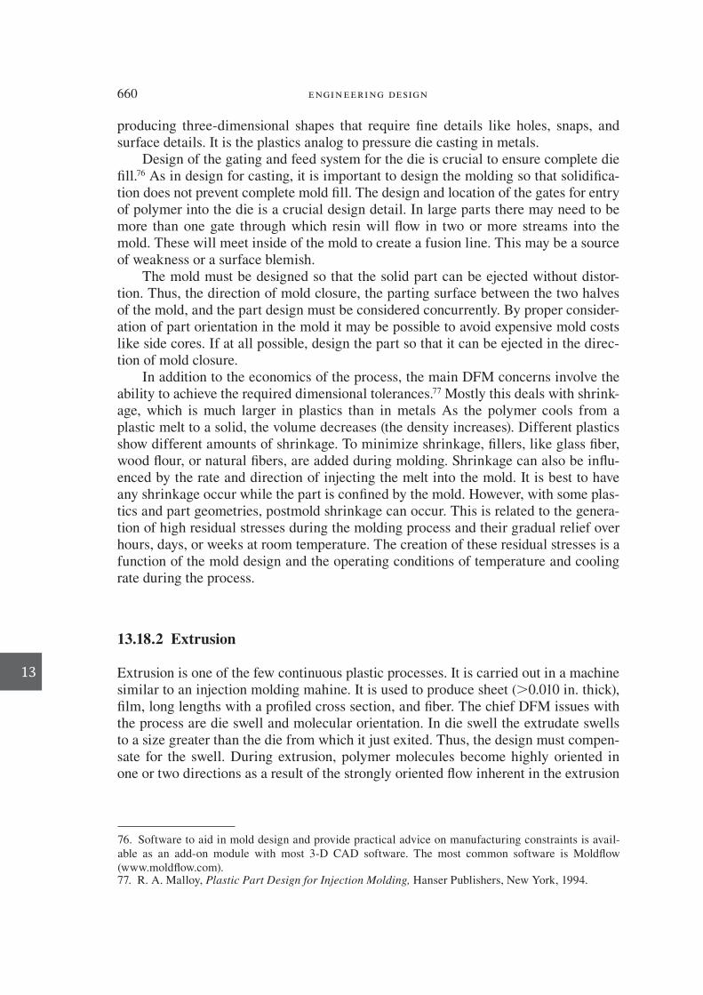
660 engineering design
13
producing three-dimensional shapes that require F ne details like holes, snaps, and surface details. It is the plastics analog to pressure die casting in metals.
Design of the gating and feed system for the die is crucial to ensure complete die F ll. 76 As in design for casting, it is important to design the molding so that solidiF ca-tion does not prevent complete mold F ll. The design and location of the gates for entry of polymer into the die is a crucial design detail. In large parts there may need to be more than one gate through which resin will C ow in two or more streams into the mold. These will meet inside of the mold to create a fusion line. This may be a source of weakness or a surface blemish.
The mold must be designed so that the solid part can be ejected without distor-tion. Thus, the direction of mold closure, the parting surface between the two halves of the mold, and the part design must be considered concurrently. By proper consider-ation of part orientation in the mold it may be possible to avoid expensive mold costs like side cores. If at all possible, design the part so that it can be ejected in the direc-tion of mold closure.
In addition to the economics of the process, the main DFM concerns involve the ability to achieve the required dimensional tolerances. 77 Mostly this deals with shrink-age, which is much larger in plastics than in metals As the polymer cools from a plastic melt to a solid, the volume decreases (the density increases). Different plastics show different amounts of shrinkage. To minimize shrinkage, F llers, like glass F ber, wood C our, or natural F bers, are added during molding. Shrinkage can also be inC u-enced by the rate and direction of injecting the melt into the mold. It is best to have any shrinkage occur while the part is conF ned by the mold. However, with some plas-tics and part geometries, postmold shrinkage can occur. This is related to the genera-tion of high residual stresses during the molding process and their gradual relief over hours, days, or weeks at room temperature. The creation of these residual stresses is a function of the mold design and the operating conditions of temperature and cooling rate during the process.
13.18.2 Extrusion
Extrusion is one of the few continuous plastic processes. It is carried out in a machine similar to an injection molding mahine. It is used to produce sheet (.0.010 in. thick), F lm, long lengths with a proF led cross section, and F ber. The chief DFM issues with the process are die swell and molecular orientation. In die swell the extrudate swells to a size greater than the die from which it just exited. Thus, the design must compen-sate for the swell. During extrusion, polymer molecules become highly oriented in one or two directions as a result of the strongly oriented C ow inherent in the extrusion
76 . Software to aid in mold design and provide practical advice on manufacturing constraints is avail-able as an add-on module with most 3-D CAD software. The most common software is MoldC ow (www.moldC ow.com). 77. R. A . Malloy , Plastic Part Design for Injection Molding, Hanser Publishers, New York , 1994 .
die37039_ch13.indd 660 2/25/08 7:00:11 PM

chapter 13: Design for Manufactur ing 661
13
process. When molecular orientation is controlled, it can improve the properties of the material.
13.18.3 Blow Molding
Blow molding produces hollow products. A heated thermoplastic tube (called a pari-son) is held inside a mold and is expanded under air pressure to match the inner con-tour of the mold. The part cools, hardens, and is ejected from the mold. The process produces a part that is dimensionally deF ned on its external dimensions, but the inte-rior surfaces are not controlled. Examples are milk bottles and automotive fuel tanks. The process does not lend itself to incorporating design details such as holes, sharp corners, or narrow ribs.
13.18.4 Rotational Molding
Like blow molding, rotational molding produces a hollow part. Rotational molding uses a F ne TP powder that is placed inside a hollow, heated metal mold. The mold is slowly rotated about two perpendicular axes. Gravity rather than centrifugal force causes even coating of the mold surface. While still rotating, the mold is cooled and the part solidiF es and hardens. Rotational molding can produce large parts, like tanks up to 500 gal capacity. Since it is a low-pressure process and the plastic is not forced through narrow channels, rotational molding does not induce a signiF cant amount of residual stress. Therefore, parts made by rotational molding exhibit a high degree of dimensional stability.
13.18.5 Thermoforming
Thermoforming, or vacuum forming, is a sheet forming process in which a TP sheet is clamped to a mold and heated to soften it, and a vacuum is applied to draw the sheet into the contour of the mold. When the sheet cools, it will retain the shape of the mold. Traditionally, thermoforming is done with only a single mold, but for more precise control of dimensions, two matching mold halves are used, as is done in sheet metal forming.
13.18.6 Compression Molding
The oldest plastics process is compression molding. It is similar to powder metallurgy. A preform of polymer, usually TS, is placed in a heated mold cavity and a plunger applies pressure to force the polymer to F ll the mold cavity. The plastic is allowed to cure and is then ejected from the mold. Because the amount of C ow is much less than in injection molding or extrusion, the level of residual stress in the part is low.
die37039_ch13.indd 661 2/25/08 7:00:12 PM

662 engineering design
13
A variation of compression molding is transfer molding . In this process the plas-tic is preheated in a transfer mold and then “shot” into the mold as a viscous liquid with a transfer ram. The ram holds the plastic under pressure until it begins to cure. Then the ram retracts, and the part completes its cure cycle and is ejected. Compres-sion molding has a cycle time of 40 to 300 s, while for transfer molding the cycle time is 30 to 150 s. Also, because a liquid plastic enters the mold in transfer molding it is possible to mold in inserts or to encapsulate parts. However, parts made this way have sprues and runners which must be trimmed and which result in lower yield of material.
13.18.7 Casting
Plastics are cast much less frequently than metals. The oldest applications are the cast-ing of sheets and rods of acrylics and the “potting” of electrical components in epoxy. The development of a wider range of casting resins has led to consideration of cast-ing as a way to make prototypes and low-volume production parts. Casting produces parts with low residual stress and a high degree of dimensional stability. Because of the high viscosity (low C uidity) of polymers it is difF cult to F ll molds by gravity alone and get F ne detail without applying pressure, as in injection molding.
13.18.8 Composite Processing
The most common composite materials are plastics reinforced with glass, metal, or carbon F bers. 78 The reinforcement may be in the form of long, continuous F laments, short F bers, or C akes. TS polymers are the most common matrix materials. Except for F lament winding, as in making a rocket motor case, the F ber and the matrix are combined in some preliminary form prior to processing. Molding compounds consist of TS resin with short, randomly dispersed F bers. Sheet molding compound (SMC) is a combination of TS resin and chopped F bers rolled into a sheet about 1/4 in. thick. Bulk molding compound (BMC) consists of the same ingredients made in billet form instead of sheet. SMC is used in the lay up of large structures. BMC is used in com-pression molding. Prepreg consists of long F bers in partially cured TS resin. Prepregs are available as tape or cross-plied sheets or fabrics.
Composites are made by either open-mold or closed-mold processes. In hand la-yups, successive layers of resin and F ber are applied to the mold by hand, with the resin being rolled into the F ber. An alternative is an open-mold process in which the liquid resin and chopped glass F bers are sprayed into the surface of the mold. In bag molding, a plastic sheet or elastomer bag is clamped over the mold and pressure is ap-plied either by drawing a vacuum or with compressed air.
Closed-mold composite processing closely follows the compression molding pro-cess. Variations have evolved to better place and orient the F bers in the composite. In
78. ASM Handbook, Vol. 21, Composites, ASM International, Materials Park, OH , 2001 .
die37039_ch13.indd 662 2/25/08 7:00:12 PM

chapter 13: Design for Manufactur ing 663
13
resin transfer molding (RTM) a glass preform or mat is placed in the mold and a TS resin is transferred into the cavity under moderate pressure to impregnate the mat.
13.18.9 DFM Guidelines for Plastics Processing
The issues of designing with plastics have been discussed in Sec. 12.6. These issues chieC y result from the lower strength and stiffness of polymers compared with metals. This limits plastic parts to applications where stresses are low, and to parts designed with many internal stiffening features. In considering DFM it must be recognized that (1) polymers have much higher coefF cients of thermal expansion and (2) much lower thermal conductivity than metals. The F rst issue means that molds must be carefully designed to achieve tight tolerances. The second issue means that because of slower heat conduction, the time for the part to cool from the melt to a solid object that can be ejected from the mold is too long to result in a desirably short cycle time. This drives the design for many plastic parts to have thin walls, usually less than 10 mm.
Since many of the design for manufacturing guidelines are common to all plastics processes, we have consolidated them here.
The wall is the most important design feature of the plastic part. The wall thickness should not vary greatly within the part. The nominal wall thickness will vary from about 4 to 30 mm depending on the process and the plastic. The rate of change of the thickness of the nominal wall should be gradual to ensure mold F lling. Avoid thick walls. They require more plastic, but more importantly, they reduce the cycle time by requiring longer time until the part is rigid enough to be ejected from the mold.
The typical projections from the inside surface of a molded wall are ribs, webs, and bosses. Ribs and webs are used to increase stiffness rather than increasing wall thickness. A rib is a piece of reinforcing material between two other features that are more or less perpendicular. A web is a piece of bracing material between two features that are more or less parallel. A boss is a short block of material protruding from a wall which is used to drive a screw through or to support something in the design. Ribs should be made slightly thinner than the walls they reinforce in order to avoid sink marks (depressions) on the outside wall.
It is important to design into a part as many features (e.g., holes, countersinks to re-ceive fasteners, snap F ts, and living hinges) as are needed rather than adding them as secondary operations. A big part of the attractiveness of plastic manufacture is that it minimizes the need for secondary operations.
Part design and process selection affect the residual stresses formed in the part. These stresses arise from inhomogeneous C ow as the polymer molecules C ow through the passages of the mold. Generous radii, higher melt temperatures (which result in longer cycle time), and processes which minimize polymer C ow result in lower residual stresses. Lower residual stresses lead to better dimensional stability.
Plastic parts are often used in consumer products where appearance is of great im-portance. An attractive feature of plastics is that they can be colored by adding color concentrates when compounding the polymer resin. The surface roughness of a molded part will reproduce the surface F nish of the mold. By etching the surface
●
●
●
●
●
die37039_ch13.indd 663 2/25/08 7:00:12 PM

664 engineering design
13
of the mold, letters or logos that protrude about 0.01 mm above the surface of the part can be produced. It is much more expensive to mold depressed letters on the part, and this should be avoided if possible.
As in forging and casting, the parting line should be chosen to avoid unnecessary complexity of the mold. Perfect mating of the parting surfaces is difF cult to achieve when they are not C at. This results in a small C ash all of the way around the perim-eter of the part. If the C ash is small due to good placement of the parting line it may be removed by tumbling, rather than a more expensive machining process. Avoid undercuts since they will require expensive movable inserts and cores.
Tight radii can be molded but generous radii allow for better polymer C ow, lon-ger mold life, and lower stress concentrations. The minimum radii should be 1 to 1.5 mm. However, large radii lead to hot spots and sinks.
Molded parts require a taper (draft angle) to remove the parts. The draft on exterior surfaces is a modest 0.5 to 2 degrees, with larger allowance on ribs and bosses.
Metal inserts are often molded in plastic parts to provide functions such as screw attachments or electrical binding posts. The C ow in these regions of the mold must be carefully designed to prevent weld lines. A weld line is formed when the fronts of two or more melt streams meet each other and fail to achieve complete intermo-lecular penetration. Often there is air trapped by the meeting of the C ow streams. This reduces the mechanical properties in the region and affects the appearance of the surface of the part. Since there is no adhesion between the surface of metals and plastics, it is important to provide mechanical locking features, like knurling, for metal inserts in plastics.
13.19
SUMMARY
This chapter completes the core theme of the book that design, materials selection, and processing are inseparable. Decisions concerning the manufacturing of parts should be made as early as possible in the design process-certainly in embodiment design. We recognize that there is a great deal of information that the designer needs to intelligently make these decisions. To aid in this the chapter provides:
An overview of the most commonly used manufacturing processes, with emphasis on the factors that need to be considered in design for manufacture
References to a carefully selected set of books and handbooks that will provide both in-depth understanding of how the processes work and detailed data needed for design
An introduction to several simple methodologies for ranking manufacturing pro-cesses on a unit cost basis that can be used early in the design process
Reference to some of the most widely used computer simulation tools for design for assembly and design for manufacturing
A material and a process for making a part must be chosen at the same time. The overall factor in deciding on the material and the manufacturing process is the cost to
●
●
●
●
●
●
●
●
die37039_ch13.indd 664 2/25/08 7:00:12 PM

chapter 13: Design for Manufactur ing 665
13
make a quality part. When making a decision on the material, the following factors must be considered:
Material composition: grade of alloy or plastic Cost of material Form of material: bar, tube, wire, strip, plate, pellet, powder, etc. Size: dimensions and tolerance Heat-treated condition Directionality of mechanical properties (anisotropy) Quality level: control of impurities, inclusions, cracks, microstructure, etc. Ease of manufacture: workability, weldability, machinability, etc. Ease of recycling
The decision on the manufacturing process will be based on the following factors:
Unit cost of manufacture Life cycle cost per unit Quantity of parts required Complexity of the part, with respect to shape, features, and size Compatibility of the process for use with candidate materials Ability to consistently make a defect-free part Economically achievable surface F nish Economically achievable dimensional accuracy and tolerances Availability of equipment Lead time for delivery of tooling Make-buy decision. Should we make the part in-house or purchase from a supplier?
Design can decisively inC uence manufacturing cost. That is why we must adopt methods to bring manufacturing knowledge into the embodiment design. An inte-grated product design team that contains experienced manufacturing people is a very good way of doing this. Design for manufacture guidelines is another way. Some gen-eral DFM guidelines are:
Minimize total number of parts in a design. Standardize components. Use common parts across product lines. Design parts to be multifunctional. Design parts for ease of manufacture. Avoid too-tight tolerances. Avoid secondary manufacturing and F nishing operations. Utilize the special characteristics of a process.
Experience has shown that a good way to proceed with DFM is to F rst do a rigor-ous design for assembly (DFA) analysis in an attempt to reduce part count. This will trigger a process of critical examination that can be followed up by what-if exercises on critical parts to drive down manufacturing cost. Use manufacturing simulation software to guide part design in improving parts for ease of manufacture and reducing tooling costs.
●
●
●
●
●
●
●
●
●
●
●
●
●
●
●
●
●
●
●
●
●
●
●
●
●
●
●
●
die37039_ch13.indd 665 2/25/08 7:00:13 PM
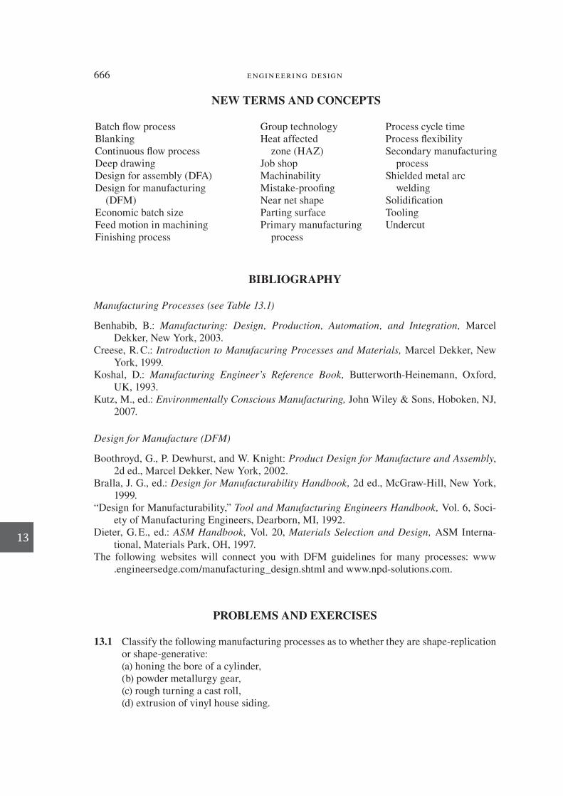
666 engineering design
13
BIBLIOGRAPHY
Manufacturing Processes (see Table 13.1)
Benhabib , B .: Manufacturing: Design, Production, Automation, and Integration, Marcel Dekker, New York , 2003 .
Creese , R. C .: Introduction to Manufacuring Processes and Materials, Marcel Dekker, New York , 1999 .
Koshal , D .: Manufacturing Engineer’s Reference Book, Butterworth-Heinemann, Oxford, UK , 1993 .
Kutz , M ., ed.: Environmentally Conscious Manufacturing, John Wiley & Sons, Hoboken, NJ , 2007 .
Design for Manufacture (DFM)
Boothroyd , G ., P . Dewhurst , and W . Knight : Product Design for Manufacture and Assembly , 2d ed., Marcel Dekker, New York , 2002 .
Bralla , J. G ., ed.: Design for Manufacturability Handbook, 2d ed., McGraw-Hill, New York , 1999 .
“Design for Manufacturability ,” Tool and Manufacturing Engineers Handbook, Vol. 6, Soci-ety of Manufacturing Engineers, Dearborn, MI , 1992 .
Dieter , G. E ., ed.: ASM Handbook, Vol. 20, Materials Selection and Design, ASM Interna-tional, Materials Park, OH , 1997 .
The following websites will connect you with DFM guidelines for many processes: www.engineersedge.com/manufacturing_design.shtml and www.npd-solutions.com.
PROBLEMS AND EXERCISES
13.1 Classify the following manufacturing processes as to whether they are shape- replication or shape-generative:
(a) honing the bore of a cylinder, (b) powder metallurgy gear, (c) rough turning a cast roll, (d) extrusion of vinyl house siding.
NEW TERMS AND CONCEPTS
Batch C ow process Group technology Process cycle time Blanking Heat affected Process C exibilityContinuous C ow process zone (HAZ) Secondary manufacturing Deep drawing Job shop process Design for assembly (DFA) Machinability Shielded metal arcDesign for manufacturing Mistake-prooF ng welding (DFM) Near net shape SolidiF cationEconomic batch size Parting surface Tooling Feed motion in machining Primary manufacturing Undercut Finishing process process
die37039_ch13.indd 666 2/25/08 7:00:13 PM

chapter 13: Design for Manufactur ing 667
13
13.2 A small hardware F tting is made from free-machining brass. For simplicity, consider that the production cost is the sum of three terms: (1) material cost, (2) labor costs, and (3) overhead costs. Assume that the F tting is made in production lots of 500, 50,000, and 5 3 10 6 pieces by using, respectively, an engine lathe, a tracer lathe, and an au-tomatic screw machine. Schematically plot the relative distribution of the cost due to materials, labor, and overhead for each of the production quantities.
13.3 Product cycle time is the time it takes for raw materials to be transformed into a F nished product. A F rm makes 1000 products per day. Before it is sold, each product represents $200 in materials and labor.
(a) If the cycle time is 12 days, how many dollars are tied up with in-process inven-tory? If the company’s internal interest rate is 10 percent, what is the annual cost due to in-process inventory?
(b) If the cycle time is reduced to 8 days as a result of process improvement, what is the annual cost saving?
13.4 You are the designer of a crankshaft for an automotive engine. You have decided to make this part from nodular cast iron using a casting process. During design you con-sult frequently with an experienced manufacturing engineer from the foundry where the part will be made. What design factors determine the manufacturing cost? Which of the costs are chieC y determined by the foundry and which by the designer?
13.5 Determine the shape complexity for a part with shape R0 in Fig. 13.6, and compare with shape R2. For shape R0 the diameter is 10 mm and the length is 30 mm. For shape R2 the overall length is 30 mm and the length of each shoulder is 10 mm. The large diameter is 10 mm and the small diameter is 6 mm. Use Eq. (13.1) to determine shape complexity. The tolerance on each dimension is !0.4 mm.
13.6 Give four metrics that could be used to measure the complexity of an assembly operation.
13.7 Examine the processes in Example 13.2. One of the processes that was rejected in the second round of decision making has great potential for making the integral bladed hub for the fan from an aluminum alloy. This process selection would have required a creative design for the die that might have required considerable development time and cost. Identify the process, and brieC y describe what technical issues prevented its selection.
Another approach is to abandon the concept that the hub and blades should be made as an integral piece. Instead, think about making the part as separate pieces to be assembled. What manufacturing processes does this open up for consideration?
13.8 Make an early design stage estimate of the manufacturing cost of the cylinder with the conical end shown in category Al in Fig. 13.18. This part must be resistant to mild sul-furic acid attack to a temperature of 200°F. It must withstand 90 psi internal pressure. The wall thickness is 0.80 !0.01 mm. The surface F nish is 0.5 mm. A total of 1000 parts is needed annually.
13.9 Make a brief literature study of the hot isostatic process (HiP). Discuss the mechanics of the process, its advantages, and its disadvantages. Think broadly about how HIPing can improve more conventional processes, and how it can impact design.
die37039_ch13.indd 667 2/25/08 7:00:13 PM

668 engineering design
13
13.10 The limiting draw ratio, the ratio of the diameter of the blank to the diameter of the deep drawn cup, is generally less than 2 for metal sheets. How then is a two-piece soft drink can made? A two-piece can is one that does not have a soldered longitudinal seam. The two parts of the can are the cylindrical can body and the top.
13.11 A manufacturing process to make a product consists of 10 separate processes. A mis-take occurs in each process on average of once every 10,000 part produced. What is the product defect rate, expressed in parts per million (ppm)?
13.12 What kind of mistake-prooF ng device or assembly method would you suggest using the following situations?
(a) A check that the required number of bolts are available for assembling a product.
(b) A count that the proper number of holes has been drilled in a plate.
(c) Insurance that three wires are connected to the proper terminals.
(d) A simple method to ensure that a product identiF cation label has not been glued upside down.
(e) A simple method to ensure that a plug is inserted in the proper orientation in an electrical plug.
13.13 As a team project, create a table comparing the plastic processing processes listed in Sec. 13.18. Develop your own list of process characteristics that are generic to all plastic processing processes. Include a clear schematic drawing of the equipment and tooling, along with a description of how the process works.
die37039_ch13.indd 668 2/25/08 7:00:13 PM

14
669
14
14
RISK, RELIABILITY, AND SAFETY
14.1 INTRODUCTION
We start this chapter by de0 ning terms that are often confused in the public mind but actually have precise technical meanings. A hazard is the potential for human, prop-erty, or environmental damage. A cracked steering linkage, a leaking fuel line, or a loose step all represent hazards. Another term for a hazard is an unsafe condition, a condition which, if not corrected, can reasonably be expected to result in failure and/or injury. A hazard is not a function of probability. It is a function of the consequence of the causal factors.
A risk is the likelihood, expressed either as a probability or as a frequency, of a hazard’s materializing. Risk is part of our individual existence and that of society as a whole. As young children we were taught about risks. “Don’t touch the stove.” “Don’t chase the ball into the street.” As adults we are made aware of the risks of society in our everyday newspaper and newscast. Thus, depending upon the particular week, the news makes us concerned about the risk of all-out nuclear war, a terrorist attack, or an airplane crash. The list of risks in our highly complex technological society is endless.
Table 14.1 lists the six classes of hazards to which society is subject. We can see that categories 3 and 4 are directly within the realm of responsibility of the engineer and categories 2, 5, and possibly 6 provide design constraints in many situations. Risk exists only when a hazard exists and something of value is exposed to the hazard.
Risk assessment has become increasingly important in engineering design as the complexity of engineering systems has increased. The risks associated with en-gineering systems do not arise because risk avoidance procedures were ignored in the design. One category of risks arises from external factors that were considered acceptable at the time of design but which subsequent research has revealed to be a health or safety hazard. A good example is the extensive use of sprayed asbestos coat-ing as an insulation and 0 re barrier before the toxicity of asbestos 0 bers was known.
die37039_ch14.indd 669 2/25/08 7:01:04 PM

670 engineering design
14
A second category of risks comes from abnormal conditions that are not a part of the basic design concept in its normal mode of operation. Usually these abnormal events stop the operation of the system without harming the general public, although there may be danger to the operators. Other systems, such as passenger aircraft or a nuclear power plant, pose a potential risk and cost to the larger public. Risks in engineering systems are often associated with operator error. Although these should be designed for using mistake-proo0 ng methods, Sec. 13.8, it is dif0 cult to anticipate all possible future events. This topic is discussed in Secs. 14.4 and 14.5. Finally, there are the risks associated with design errors and accidents. Clearly, these should be eliminated, but since design is a human activity, errors and accidents will occur. 1
Most reasonable people will agree that society is not risk-free and cannot be made so. 2 However, an individual’s reaction to risk depends upon three main factors: (1) whether the person feels in control of the risk or whether the risk is imposed by some outside group, (2) whether the risk involves one big event (like an airplane crash) or many small, separate occurrences, and (3) whether the hazard is familiar or is some strange, puzzling risk like a nuclear reactor. Through the medium of mass communi-cations the general public has become better informed about the existence of risks in society, but they have not been educated concerning the need to accept some level of risk and to balance risk avoidance against cost. It is inevitable that there will be con-b ict between various special-interest groups when trying to decide on what constitutes an acceptable risk.
Reliability is a measure of the capability of a part or a system to operate without failure in the service environment. It is always expressed as a probability; e.g., a reli-ability of 0.999 implies that there is probability of failure of 1 part in every 1000. The mathematics of reliability is introduced in Sec. 14.3.
Safety is relative protection from exposure to hazards. A thing is safe if its risks are judged to be acceptable. 3 Therefore, two different activities are involved in determining
TABLE 14.1
Classi+ cation of Societal Hazards
Category of Hazard Examples
1. Infections and degenerative diseases Inb uenza, heart disease, AIDS
2. Natural disasters Earthquakes, b oods, hurricanes
3. Failure of large technological systems Failure of dams, power plants, aircraft, ships, buildings
4. Discrete small-scale accidents Automotive accidents, power tools, consumer and sport
goods
5. Low-level, delayed-effect hazards Asbestos, PCB, microwave radiation, noise
6. Sociopolitical disruption Terrorism, nuclear weapons proliferation, oil embargo
From W. W. Lowrance, in R. C. Schwing and W. A. Albus (eds.), Social Risk Assessment, Plenum Press, New
York, 1980.
1. T . Kletz , An Engineer’s View of Human Error, 3d ed., Taylor & Francis, New York , 2006 . 2. E . Wenk , Tradeoffs: Imperatives of Choice in a High-Tech World, Johns Hopkins University Press,
Baltimore , 1986 .
3. W. W . Lowrance , Of Acceptable Risk, William Kaufman, Inc., Los Altos, CA , 1976 .
die37039_ch14.indd 670 2/25/08 7:01:05 PM

chapter 14: Risk, Rel iabil ity, and Safety 671
14
how safe a design is: (1) a risk assessment, which is a probabilistic activity, and (2) a judgment of the acceptability of that risk, which is a societal value judgment.
14.1.1 Regulation as a Result of Risk
In a democracy, when the public perception of a risk reaches suf0 cient intensity, legis-lation is enacted to control the risk. That usually means the formation of a regulatory commission that is charged with overseeing the regulatory act. In the United States the 0 rst regulatory commission was the Interstate Commerce Commission (ICC). The fol-lowing federal organizations have a major role to play in some aspects of technical risk:
Consumer Product Safety Commission (CPSC) Environmental Protection Agency (EPA) Federal Aviation Agency (FAA) Federal Highway Administration (FHA) Federal Railway Administration (FRA) Nuclear Regulatory Commission (NRC) Occupational Safety and Health Administration (OSHA)
Some of the federal laws concerning product safety are listed in Table 14.2. The rapid acceleration of interest in consumer safety legislation is shown by the dates of enactment of these regulatory laws. Once a federal regulation becomes of0 cial it has the force of law. In the United States, some 60 federal agencies issue more than 1800 regulations a year; the Code of Federal Regulations (CFR), contains more than 130,000 pages. 4
TABLE 14.2
A Sample of Federal Laws Concerning
Produc t Safety
Year Legislation
1893 Railroad Appliance Safety Act
1938 Food, Drug, and Cosmetic Act
1953 Flammable Fabrics Act
1960 Federal Hazardous Substance Act
1966 National Traf0 c and Motor Vehicle Safety Act
1968 Fire Research and Safety Act
1969 Child Protection and Toy Safety Act
1970 Poison Prevention Packaging Act
1970 Lead-Based Paint Poison Prevention Act
1970 Occupational Safety and Health Act
1971 Federal Boat Safety Act
1972 Consumer Product Safety Act
4. The Economist, Aug. 2, 1997, p. 2; for CFR at www.gpo.gov/nara/cfr/incex.html
die37039_ch14.indd 671 2/25/08 7:01:05 PM

672 engineering design
14
Legislation has the important result that it charges all producers of a product with the cost of complying with the product safety regulations. Thus, we are not faced with the situation in which the majority of producers spend money to make their product safe but an unscrupulous minority cuts corners on safety to save on cost. However, in complex engineering systems it may be very dif0 cult to write regulations that do not conb ict with each other and work at cross purposes. The automobile is a good ex-ample. 5 Here, separate agencies have promulgated regulations to inb uence fuel econ-omy, exhaust emissions, and crash safety. The law to control emissions also reduces fuel ef0 ciency by 7.5 percent, but the fuel ef0 ciency law has forced the building of smaller cars that have increased crash fatalities by an additional 1400 per year. The need for a strong technical input into the regulatory process should be apparent from this example.
A common criticism of the regulatory approach is that decisions are often made arbitrarily. That is understandable when we consider that a regulatory agency often has a congressional mandate to protect the public from “unreasonable risk.” Since there usually are no widely agreed-on de0 nitions of unreasonable risk, the regulators are accused of being hostile to or soft on the regulated industry, depending upon the individual’s point of view. Sometimes the regulating agency speci0 es the technology for meeting the target level of risk. This removes the incentive for innovation in devel-oping more effective methods of controlling the risk.
14.1.2 Standards
Design standards were 0 rst considered in Sec. 1.7. Here we discussed the difference between a code and a standard, the different kinds of standards, and the types of organizations that develop standards. In Sec. 5.8 standards were discussed for their value as sources of information. In this section we consider standards and codes more broadly from the viewpoint of the role they play in minimizing risk. Standards are among the most important ways in which the engineering profession makes sure that society receives a minimum level of safety and performance.
The role that standards play in protecting public safety was 0 rst shown in the United States in the middle of the 19th century. This was a time of rapid adoption of steam power on railroads and in ships. The explosion of steam boilers was an all-too-frequent occurrence, until the ASME developed the Boiler and Pressure Vessel Code that prescribed detailed standards for materials, design, and construction. The ASME Boiler Code was quickly adopted as law by the individual states. Other examples of public safety standards are 0 re safety and structural codes for buildings and codes for the design, construction, maintenance, and inspection of elevators.
Other standards protect the general health and welfare. Examples are emission standards for cars and power plants to protect public health by minimizing air pollu-tion, and standards on the discharge of efb uents into rivers and streams.
5. L. B . Lave , Science , vol. 212, pp. 893–99 , May 22, 1981 .
die37039_ch14.indd 672 2/25/08 7:01:05 PM
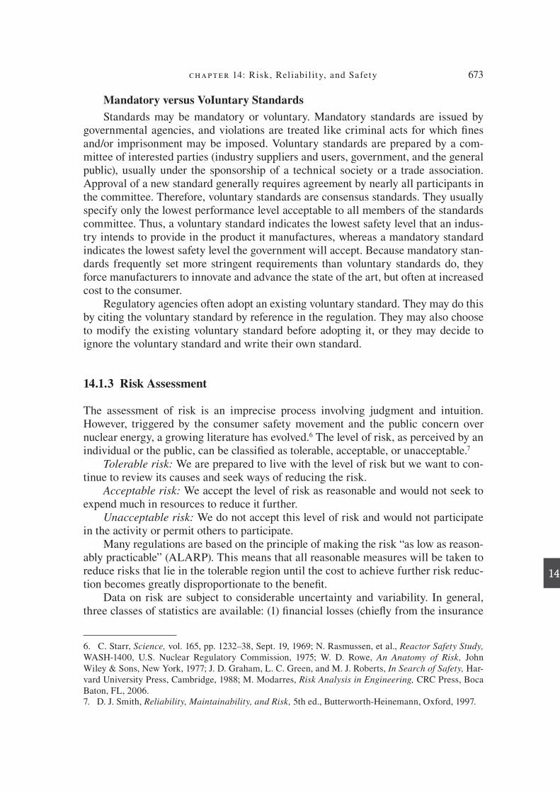
chapter 14: Risk, Rel iabil ity, and Safety 673
14
Mandatory versus VoIuntary Standards
Standards may be mandatory or voluntary. Mandatory standards are issued by governmental agencies, and violations are treated like criminal acts for which 0 nes and/or imprisonment may be imposed. Voluntary standards are prepared by a com-mittee of interested parties (industry suppliers and users, government, and the general public), usually under the sponsorship of a technical society or a trade association. Approval of a new standard generally requires agreement by nearly all participants in the committee. Therefore, voluntary standards are consensus standards. They usually specify only the lowest performance level acceptable to all members of the standards committee. Thus, a voluntary standard indicates the lowest safety level that an indus-try intends to provide in the product it manufactures, whereas a mandatory standard indicates the lowest safety level the government will accept. Because mandatory stan-dards frequently set more stringent requirements than voluntary standards do, they force manufacturers to innovate and advance the state of the art, but often at increased cost to the consumer.
Regulatory agencies often adopt an existing voluntary standard. They may do this by citing the voluntary standard by reference in the regulation. They may also choose to modify the existing voluntary standard before adopting it, or they may decide to ignore the voluntary standard and write their own standard.
14.1.3 Risk Assessment
The assessment of risk is an imprecise process involving judgment and intuition. However, triggered by the consumer safety movement and the public concern over nuclear energy, a growing literature has evolved. 6 The level of risk, as perceived by an individual or the public, can be classi0 ed as tolerable, acceptable, or unacceptable. 7
Tolerable risk: We are prepared to live with the level of risk but we want to con-tinue to review its causes and seek ways of reducing the risk.
Acceptable risk: We accept the level of risk as reasonable and would not seek to expend much in resources to reduce it further.
Unacceptable risk: We do not accept this level of risk and would not participate in the activity or permit others to participate.
Many regulations are based on the principle of making the risk “as low as reason-ably practicable” (ALARP). This means that all reasonable measures will be taken to reduce risks that lie in the tolerable region until the cost to achieve further risk reduc-tion becomes greatly disproportionate to the beneB t.
Data on risk are subject to considerable uncertainty and variability. In general, three classes of statistics are available: (1) B nancial losses (chieH y from the insurance
6. C . Starr , Science, vol. 165, pp. 1232–38 , Sept. 19, 1969 ; N . Rasmussen , et al., Reactor Safety Study,
WASH-1400, U.S. Nuclear Regulatory Commission, 1975 ; W. D . Rowe , An Anatomy of Risk, John
Wiley & Sons, New York , 1977 ; J. D . Graham , L. C . Green , and M. J . Roberts , In Search of Safety, Har-
vard University Press, Cambridge , 1988 ; M . Modarres , Risk Analysis in Engineering , CRC Press, Boca
Baton, FL , 2006 . 7. D. J . Smith , Reliability, Maintainability, and Risk, 5th ed., Butterworth-Heinemann, Oxford , 1997 .
die37039_ch14.indd 673 2/25/08 7:01:06 PM

674 engineering design
14
industry), (2) health information, and (3) accident statistics. Usually the data are dif-ferentiated between fatalities and injuries. Risk is usually expressed as the probability of the risk of a fatality per person per year. A risk that exceeds 10 23 fatalities per per-son per year is generally considered unacceptable, while a rate that is less than 10 25 is not of concern to the average person. 8 The range 10 23 to 10 25 is the tolerable range. However, an individual’s perception of risk depends upon the circumstances. If the risk is voluntarily assumed, like smoking or driving a car, then there is a greater ac-ceptance of the risk than if the risk was assumed involuntarily, as with traveling in a train or breathing secondhand smoke. There is a large difference between individual risk and societal risk. While 10 23 is the boundary where unacceptable risk begins for a single voluntary death, the acceptable fatality rate shifts to about 10 25 if 100 deaths are involved. Table 14.3 gives some generally accepted fatality rates for a variety of risks.
14.2 PROBABILISTIC APPROACH TO DESIGN
Conventional engineering design uses a deterministic approach. It disregards the fact that material properties, the dimensions of the parts, and the externally applied loads vary statistically. In conventional design these uncertainties are handled by applying a factor of safety. In critical design situations such as aircraft, space, and nuclear ap-plications, it is often necessary to use a probabilistic approach to better quantify un-certainty and thereby increase reliability. 9
TABLE 14. 3
Fatality Rate
Cause of Fatality Fatality per Person per Year
Smoking (20 per day) 5 3 1023
Cancer, in general 3 3 1023
Race car driving 1 3 1023
Motor vehicle driving 3 3 1024
Fires 4 3 1025
Poison 2 3 1025
Industrial machinery 1 3 1025
Air travel 9 3 1026
Railway travel 4 3 1026
California earthquake 2 3 1026
Lightning 5 3 1027
9. E. B . Haugen , Probabilistic Mechanical Design, Wiley-Interscience, Hoboken, NJ , 1980 ; J. N . Siddal ,
Probabilistic Engineering Design, Marcel Dekker, New York , 1983 .
8. D. J . Smith , Reliability, Maintainability, and Risk, 5th ed., Butterworth-Heinemann, Oxford , 1997 .
die37039_ch14.indd 674 2/25/08 7:01:06 PM

chapter 14: Risk, Rel iabil ity, and Safety 675
14
There are three approaches for incorporating probabilistic effects in design. In order of increasing sophistication they are: the use of a factor of safety, the use of the absolute worst case design, and the use of probability in design. We will present the probabilistic approach B rst, and then show how the other approaches can be folded in.
14.2.1 Basic Probability Using the Normal Distribution
Many physical measurements follow the symmetrical, bell-shaped curve of the nor-mal, or Gaussian frequency distribution. The distributions of yield strength, tensile strength, and reduction of area from the tension test follow the normal curve to a suit-able degree of approximation. The equation of the normal curve is
f xx( ) = −
−
1
2
1
2
2
σ π
µσ
exp (14.1)
where f ( x ) is the height of the frequency curve corresponding to an assigned value x , m is the mean of the population, and s is the standard deviation of the population. 10 The normal distribution extends from x 5 2` to x 5 1` and is symmetrical about the population mean m. The existence of negative values and long “tails” makes the normal distribution a poor model for certain engineering problems.
In order to place all normal distributions on a common basis in a standardized way, the normal curve frequently is expressed in terms of the standard normal vari-
able or the z variable.
zx
=− µσ
(14.2)
Now, the equation of the standard normal curve becomes
f zz( ) = −
1
2 2
2
πexp (14.3)
Figure 14.1 shows this standardized normal curve, where m 5 0 and s 5 1. The total area under the curve is unity. The probability of a value of z falling between z 5 2` and a speciB ed value of z is given by the area under the curve. Probability is the numerical measure of likelihood of an event. The probability, P , is bounded be-tween P 5 0 (an impossible event) and P 5 1 (a certain event).
The area under the curve from 2` to z 5 21.0 is 0.1587, so the probability of a value falling into that interval is P 5 0.l587, or 15.87 percent. Since the curve is sym-metric, the probability of a value falling into the interval z 5 2l to z 5 l or m ! s is 1.0000 22(0.1587) 5 0.6826. In a similar way it can be shown that m ! 3s encom-passes 99.73 percent of all values.
Some typical values for the area under the z curve are listed in Table 14.4. More complete values will be found in Appendix B. For example, if z 5 23.0 the prob-ability of a value being less than z is 0.0013 or 0.13 percent. The percentage of values
10 . DeB nitions of statistical terms can be found in Appendix A.
die37039_ch14.indd 675 2/25/08 7:01:06 PM

676 engineering design
14
greater than this z is 100 2 0.13 5 98.87 percent. The fraction of values less than z is 1/0.0013 5 1 in 769. Table 14.4 also shows that if we wanted to exclude the lowest 5 percent of the population values we would set z at 21.645.
E X A M P L E 14 . 1
A highly automated factory is producing ball bearings. The average ball diameter is 0.2152
in. and the standard deviation is 0.0125 in. These dimensions are normally distributed.
(a) What percentage of the parts can be expected to have a diameter less than 0.2500 in.?
Note that up until now we have used m and s to represent the mean and standard devia-
tion of the population. The sample values of the mean and standard deviation are given
TABLE 14.4
Areas Under Standardized Normal Frequency Curve
z 5 x M/S Area z Area
z 02` 1`
23.0 0.0013 23.090 0.001
22.0 0.0228 22.576 0.005
21.0 0.1587 22.326 0.010
20.5 0.3085 21.960 0.025
0.0 0.5000 21.645 0.050
10.5 0.6915 1,645 0.950
11.0 0.8413 1.960 0.975
12.0 0.9772 2.326 0.990
13.0 0.9987 2.576 0.995
3.090 0.999
FIGURE 14.1
Standardized normal frequency
distribution.
P(z)
0.4
0.3
0.2
0.1
z5x2"
#
23 22 21 0 1 2 3
die37039_ch14.indd 676 2/25/08 7:01:07 PM

chapter 14: Risk, Rel iabil ity, and Safety 677
14
by x_
and s . In this example, where we are sampling literally millions of balls, these values
are nearly identical.
Determining the standard normal variable
zx x x
s=
−≈
−=
−=
−µσ
0 2500 0 2512
0 0125
0 0012
0 01
. .
.
.
. 2250 096= − .
From Appendix B, P ( z , 20.09) 5 0,4641 and P ( z , 20.10) 5 0.4602. Interpolating, the
area under the z distribution curve at z 5 20.096 is 0.4618. Therefore, 46.18 percent of
the ball bearings are below 0.2500 in. diameter.
(b) What percentage of the balls are between 0.2574 and 0.2512 in.?
z
z
=−
=
=−
=
0 2512 0 2512
0 01250 0
0 2574 0 2512
0 0125
0 0062
0 012
. .
..
. .
.
.
. 550 50= + .
Area under curvefrom to is 0.5000.− =∞ z 0
Area under curvefrom
to is 0.6915− =∞ z 0 5.
Therefore, percentage of ball diameters in interval 0.2512 to 0.2574 is 0.6915 2 0.5000
5 0.1915 or 19.15 percent.
14.2.2 Sources of Statistical Tables
All statistical texts contain tables for the z distribution, the conB dence limits of the mean, and the t and f distributions, but tables of more esoteric statistics often needed in engineering may be more elusive. Here we mention two convenient sources of sta-tistical tables and information.
The Microsoft spreadsheet program Excel provides access to many special math-ematical and statistical functions. To display this menu of functions, click on the In-sert Function button, f x , on the formula bar at the top of a spreadsheet and search in the function box for the special function you might need. Click on the name of the function for a description and example of how to use it. Table 14.5 is a short listing of some of the more useful statistical functions.
Experimental Statistics, edited by M. G. Natrella, and published by the National Bureau of Standards as Handbook 91, August 1963, is a useful compilation of sta-tistical procedures and tables. It is now available on the Internet as Engineering Statistics Handbook at www.itl.nist .gov/div898/handbook .
14.2.3 Frequency Distributions Combining Applied Stress and Material Strength
Consider a structural member subjected to a static load that develops a stress s. The variation in load or sectional area results in the distribution of stress shown in Fig. 14.2, where the mean is –s and the standard deviation 11 of the sample of stress
11 . Note that probabilistic design is at the intersection of two engineering disciplines: mechanical design
and engineering statistics. Thus, confusion in notation is a problem.
die37039_ch14.indd 677 2/25/08 7:01:08 PM

678 engineering design
14
values is s . The yield strength of the material Sy has a distribution of values given by
Sy
and s y . However, the two frequency distributions overlap, and it is possible for s , S y , which is the condition for failure. The probability of failure is given by
P P Sf y
= >( )σ (14.4)
The reliability R is deB ned as
R Pf
= −1 (14.5)
If we subtract the stress distribution from the strength distribution, we get the distri-bution Q 5 S y 2 s shown at the left in Fig. 14.2.
We now need to be able to determine the mean and standard deviation of the distribution Q constructed by performing algebraic operations on two indepen-dent random variables x and y , that is, Q 5 x ! y . Without going into statistical
Sy
sQ = 10Q = 100 Stress, ksi
Q = Sy –
s = 8 = 30
sy = 6Sy = 40
FIGURE 14.2
Distributions of yield strength S y and stress.
TABLE 14.5
Some Statistical Functions Available in Excel
Function Description of Excel Function
NORMDIST Returns the f(x) in Eq. (14.1) for given x, m and s
NORMINV Returns x in Eq. (14.1) for given f(x), m and s
NORMSDIST Returns the area under Eq. (14.3) for a given z (probability)
NORMSINV Returns the std normal variable z, given the probability (area under f(z))
LOGNORMDIST Returns the f(x) for a distribution where 1n x is normally distributed
EXPONDIST Returns the exponential distribution
GAMMADIST Returns values of the Gamma distribution (useful in Weibull distribution)
WEIBULL Returns the Weibull distribution for values of x, and shape and scale parameters
ZTEST Returns the two-tailed probability in a z test
TDIST Returns values of the t distribution
FDIST Returns values of the F distribution
FINV Returns the inverse of the F probability distribution
die37039_ch14.indd 678 2/25/08 7:01:08 PM

chapter 14: Risk, Rel iabil ity, and Safety 679
14
details, 12 the results are as given in Table 14.6. Referring now to Fig. 14.2, and using the results in Table 14.6, we see that the distribution Q 5 S y 2 s has a mean value and
Q Q= − = = + =40 30 10 6 8 102 2and σ . The part of the distribution to the left of Q 5 0 represents the area for which S y 2 s is a negative number, that is, s , S y , and fail-ure occurs. If we transform to the standard normal variable, z 5 ( x 2 m)/s, we get, at Q 5 0,
zQ
Q
=−
= − = −0 10
101 0
σ.
From a table of cumulative normal distribution we B nd that 0.16 of the area falls be-tween 2` and z 5 21. 0. Thus, the probability of failure is P f 5 0.16, and the reliabil-ity is R 5 1 2 0.16 5 0.84. Clearly, this is not a particularly satisfactory situation. If we select a stronger material with S Q
y= =50 20 ksi, and z 5 2.0. The probability of
failure now is about 0.02. Values of z corresponding to various values of failure prob-abilities are given in Table 14.7.
14.2.4 Variability in Material Properties
The mechanical properties of engineering materials exhibit variability. Fracture and fatigue properties show greater variability than the static tensile properties of yield strength and tensile strength (see Table 14.8). Most published mechanical property data do not give mean values and standard deviations. Haugen 13 has presented much of the published statistical data. MMPDS-02 Handbook presents extensive statistical
TABLE 14.6
Mean and Standard Deviation of
Independent Random Variables x and y
Algebraic Functions Mean, Q Std. Deviation
Q = C C 0
Q = Cx C x Csx
Q = x + C x C+ sx
Q = x ± yx y± σ σ
x y
2 2+
Q = xy x y x yy x
2 2 2 2σ σ+
Q = x/y x y/ x y yy x
2 2 2 21 2
2σ σ+( ) /
/
Q 5 1/x 1 / x σx
x/ 2
12. E. B . Haugen , op. cit. , pp. 26–56 . 13. E. B . Haugen , op. cit. , Chap. 8 and App. 10A and 10B.
die37039_ch14.indd 679 2/25/08 7:01:08 PM

680 engineering design
14
data for materials used in aircraft. 14 Much other statistical data resides in the B les of companies and government agencies.
Published mechanical property data without statistical attribution is usually taken to represent a mean value. If a range of values is given, the lower value is often taken to represent a conservative value for design. Although certainly not all mechanical properties are normally distributed, a normal distribution is a good B rst approxima-tion that usually results in a conservative design. When statistical data are not avail-able we can estimate the standard deviation by assuming that the upper x U and lower x L values of a sample are ! three standard deviations from the mean. Thus,
x xx x
U L
U L− = ≈−
66
σ σand s = (14.6)
TABLE 14.7
Value of z to Give Different Levels
of Probability of Failure
Probability of Failure Pf z 5 (x M)/S
1021 21.28
1022 22.33
1023 23.09
1024 23.72
1025 24.26
1026 24.75
TABLE 14.8
Typical Values of CoefS cient of Variation
Variable x Typical D
Modulus of elasticity of metals 0.05
Tensile strength of metals 0.05
Yield strength of metals 0.07
Buckling strength of columns 0.15
Fracture toughness of metals 0.15
Cycles to failure in fatigue 0.50
Design load in mechanical components 0.05–0.15
Design load in structural systems 0.15–0.25
H. R . Millwater and P. H . Wirsching , “Analysis Methods for
Probabilistic Life Assessment,” ASM Handbook, Vol. 17,
p. 251 , ASM International , Materials Park, OH, 2002 .
14. Metallic Materials Properties Development and Standardization Handbook, 5 volumes, 2005 . This
is the successor to MIL-HDBK-5 formerly published by DOD. The last (2003) version of this hand-
book can be viewed at www.mmpds.org. New versions of MMPODS can be purchased from ASM
International .
die37039_ch14.indd 680 2/25/08 7:01:09 PM

chapter 14: Risk, Rel iabil ity, and Safety 681
14
When the range of property values is not given, it is still possible to approximate the standard deviation by using the coef! cient of variation , d, which is a measure of the uncertainty of the value of the mean.
δ =s
x (14.7)
The coefB cient of variation is different for each mechanical property, but it tends to be relatively constant over a range of mean values. Thus, it is a way of estimating the standard deviation. Table 14.8 gives some values of coefB cient of variation.
E X A M P L E 14 . 2
The yield strength of a sample of 50 tensile specimens from an alloy steel is x = 130 1. ksi.
The range of yield strength values is from 115 to 145 ksi. The estimate of standard deviation,
which measures the variability in the strength values, is sx x
U L=−
=−
=6
145 115
65ksi.
Assuming that a normal distribution applies, estimate the value of yield strength which
99 percent of the yield strengths will exceed. From Table 14.4, z 1% 5 22.326, and from
Eq. (14.2)
− =−
=2 326130 1
5118 51.
..%
x and x ksi
1%
Note that if the range of yield strength had not been known, we could estimate the stan-
dard deviation from Table 14.8 and Eq. (14.7).
s x x= = × = =δ 130 1 0 07 9 1 1081
. . . ksi. Thisresults in % ..9ksi
In Example 14.2, sample values of mean and standard deviation were used to determine the probability limits. This is inaccurate unless the sample size n is very large, possibly approaching n 5 1000. This is because the sample values x and s are only estimates of the true population values m and s. The error in using sample values to estimate population values can be corrected if we used tolerance limits . Because we generally are interested in B nding the lower limit of the property, we use the one-sided tolerance limit.
x x k sL R C
= − ( ), (14.8)
To B nd k R,C statistical tables 15 we B rst need to decide on the conB dence level, c. This is usually taken as 95 percent, indicating that we have a 95 percent conB dence that the method will produce a true lower limit on the property. R is our expectation that the value of x L will be exceeded R percent of the time. Usually R is taken at 90, 95 or 99 percent. Table 14.9 gives some values of k R,C for different values of sample size n.
E X A M P L E 14 . 3
Now we redo Example 14.2 using the one-sided tolerance limit. The sample size is n 5
50, so k R,C 5 2.86 at a 95 percent conB dence level and with R 5 0.99. Then, x L 5 130.1 2
2.86(5) 5 115.8 ksi. Note that x L has been decreased from 118.5 to 115.8 ksi when we
corrected for using sample statistics instead of population statistics. If n consisted of only
10 specimens, x L would be 110.2 ksi.
15 . J. Devore and N. Farnum, Table V, Applied Statistics for Engineers and Scientists, Duxbury Press,
PaciB c Grove, CA.
die37039_ch14.indd 681 2/25/08 7:01:09 PM

682 engineering design
14
14.2.5 Probabilistic Design
We illustrate the probabilistic approach to design with the example 16 of a crank that must support a single static load P (Fig. 14.3). The shaft is considered to be a cantile-ver supported beam and is to be made from AISI 4140 steel tubing. Each design vari-able in the problem is a random variable that is assumed to be normally distributed. The mean and standard deviation ( x
_, s) for the parameters are estimated as follows:
Load lb
Yield stress
P
Sy
= ( )=
150 10
12
,
99 3 3 2. , .
,
( )= ( )
ksi
Shaft diameter mad xd d
σ nnufacturing tolerance isassumed to be
σd
x= 0 015.dd
L
L
1
2
6
4 3 32
= ±
= ±
in. 1/4 in.
in. in./
In order to prevent buckling of the tubular shaft, the allowable tube thickness is deter-mined by d / t < 100. We choose the minimum value, t 5 d /100. The moment of inertia of this cross section is I 5 0.003811 d 4 . The polar moment of inertia of the shaft is given by J 5 2 I 5 2 kd 4 .
The critical stress in the tubular shaft, which will determine the outside diameter, occurs at both top and bottom on the outside surface where it connects to the wall. The torsional stress and the bending stress are both maximum at these locations. If the yield strength S y is exceeded, failure will initiate there. Because this is a combined
16. This example is taken from a paper “Introducing Reliability Concepts in Machine Design” by J. R .
Steffen , L. T . Hayes , D. W . Wiedemeir , and S . Tennyson , 1988 ASEE Annual Conference Proceedings,
pp. 902–9 .
TABLE 14.9
One-Sided Tolerance Limit Factors
for 95% ConS dence Level
n k 90,95 k 99,95
5 3.41 5.74
10 2.35 3.98
20 1.93 3.30
50 1.65 2.86
100 1.53 2.68
500 1.39 2.48
` 1.28 2.37
Note: These apply only to normally distributed variables.
die37039_ch14.indd 682 2/25/08 7:01:10 PM

chapter 14: Risk, Rel iabil ity, and Safety 683
14
stress situation, the von Mises yield stress, S 0 , will be the controlling stress. For the geometry of this problem, this is given by
S P kd L L0
3
1
2
2
21 2
4 4 3= ( ) +( )//
The mean value for the von Mises stress is given by
x x kx x x xS P d L L d0 1 2
4 4 3 0 1364 103 2 21 2
6 3= ( ) +( ) = ( )/ . //
The standard deviation of the von Mises stress can be determined from the rela-
tionship σ σf i x
f xi
= ∂ ∂[ ( / ) ( ) ] ,/Σ 2 2 1 2 which holds when the dispersion of each ran-
dom variable, c x= σ / is less than 0.20. For the von Mises stress,
σ σ σS P d
S
P
S
d
S
L0
0
2
2 0
2
2 0
1
∂∂
+
∂∂
+
∂∂
+
∂∂
2
2 0
2
2
2
1 2
1 2
σ σL L
S
L
/
The partial derivatives are computed from the above equation for S 0 .
∂∂
= +( ) = ( )∂∂
= − +
S
PL L kd x
S
dP L L
d
0
1
2
2
21 2
3 3 3
0
1
2
2
4 3 4 0 9090 10
3 4 3
/
/ . /
221 2
4 3 4
0
1
1
3 1
2
2
21 2
4 0 4090 10
4 3
( ) = − ( )∂∂
= +( ) =−
/
/
/ . /kd x
S
L
PL
kdL L
d
117 04 10
3
44 3 8 522 10
3 3
0
2
2
3 1
2
2
21 2
3
. /
. //
( )∂∂
= +( ) = ( )−
x
S
L
PL
kdL L x
d
dd
3
L2
L1
y
z
x
P
FIGURE 14.3
Cantilever supported crank
attached to steel tube. “Re-
printed with permission from
the Proceedings of the 1988
Annual Conference of the
American Society for Engineer-
ing Education.”
die37039_ch14.indd 683 2/25/08 7:01:11 PM

684 engineering design
14
Substituting these four equations and the values for the s terms results in:
σ
S d dx x
0
82 62 10 37 64 10 2 017 106 6 6 6 6= ( ) + ( ) + (. / . / . ))
+ ( ) = ( )
/
. / . //
x
x x
d
d d
6
6 61 2
30 0709 10 11 06 10 33
We can use Fig. 14.2 to visualize the solution. We know the distribution of strength, S
y= 129 3. and s y 5 3.2, and we have just calculated the distribution of
von Mises combined stress, x x xS d S d
0 0
136 4 11 063 3= =. / . / .andσ All values are in ksi. If we set the allowable failure probability at 0.001 the corresponding value of z from Table 14.7 is 23.09. Thus, following the earlier analysis of subtracting the stress dis-tribution from the strength distribution, we get
zx
x
d
d
= − =− −( )
( ) +
3 090 129 3 136 4
3 211 06
3
2
3
21
.. . /
..
// 2
Solving for x x t xd d d
gives in.The tube thickness is then in= = =1 102 100 0 011. / . ..
14.2.6 Safety Factor
The use of a safety factor is far simpler than the preceding method, but with much less information content. Using a safety factor is a form of “derating,” but the extent of reduction from the true capacity is not known. In the usual case for static loading, the safety factor N 0 is the yield strength divided by the working stress, in this example the von Mises stress.
N S S S x
y y S0 0 0= =/ /
We can see that the safety factor is the ratio of the mean capacity to the mean load or demand. If we choose N 0 = 1. 25, then we can calculate the shaft diameter.
1 25 129 3 136 4
1 096
3. . / . /
.
= ( )=
x
x
d
din.
Since we already know the pertinent statistics from the probabilistic design calculation, we can readily determine the probability of failure associated with the choice of safety factor.
zx
x
d
d
=−
( ) + ( )
136 4 129 3
3 2 11 06
3
2 32
1 2
. / .
. . //
and on substituting x_
d 5 1.096 we compute z = 22.858, which corresponds to a fail-ure probability of about 0.002.
die37039_ch14.indd 684 2/25/08 7:01:11 PM

chapter 14: Risk, Rel iabil ity, and Safety 685
14
Some very interesting examples of the calculation of factors of safety have been given by Mischke. 17 An interesting philosophical view on the factor of safety is given by Carter. 18
14.2.7 Worst Case Design
In worst case design (WCD), the variables are set at either the lowest or largest ex-pected values. WCD, like the use of the safety factor, is an approach that accounts for the statistical nature of the design environment in a deterministic way.
Using the previous analysis for the tubular shaft under probabilistic design, fail-ure occurs when the von Mises stress equals the material yield strength, S y . Thus, the shaft diameter can be expressed by
d P kS L L
y= ( ) +( )
//
/
4 4 31
2
2
21 2
1 3
To determine whether each design variable should be at its high or low end for WCD, take the partial derivative of d with respect to that variable. Thus,
∂∂
=
+( )
d
P kSL L
y
1
44 3
1
31
2
2
21 2
1 3
/
/
PP2 3/= positive value
Similarly, we B nd that maximum values should be used for L 1 and L 2 and a minimum value for S y . The bounds on the design variables are given either as a tolerance limit, such as L 1 5 6 ! 1/4 in, or by using the 3s limit as the tolerance, e.g., P 5 150 ! 3(10). Putting the appropriate values into the equation for shaft diameter yields d min .
d =( ) + ( ){ }
( )( )
180 4 6 25 3 4 094
4 0 003811 119 700
2 21 2
. .
. ,
/11 3
1 123
/
.= ln.
Note that while the analysis is easy for WCD, this approach leads to the use of excess material.
14.3 RELIABILITY THEORY
Reliability is the probability that a system, component, or device will perform without failure for a speciB ed period of time under speciB ed operating conditions. The dis-cipline of reliability engineering basically is a study of the causes, distribution, and
17. C. R . Mischke , “ Some Guidance of Relating Factor of Safety to Risk of Failure, ” ASME Paper 86-WA/DE-22.
18. A. D. S. Carter, Mechanical Reliability and Design, pp. 11–16, John Wiley & Sons, New York, 1997.
die37039_ch14.indd 685 2/25/08 7:01:11 PM

686 engineering design
14
prediction of failure. 19 If R ( t ) is the reliability with respect to time t , then F ( t ) is the unreliability (probability of failure) in the same time t . Since failure and nonfailure are mutually exclusive events,
R t F t( ) + ( ) = 1 (14.9)
If N 0 components are put on test, the number surviving to or at time t is N s ( t ), and the number that failed between t 5 0 and t 5 t is N f ( t ).
N t N t Ns f( ) + ( ) =
0 (14.10)
From the deB nition of reliability
R tN t
N
N t
N
s f( ) =( )
= −( )
0 0
1 (14.11)
The hazard rate, or instantaneous failure rate, is the number of failures per unit time per the number of items exposed for the same time.
h tdN t
dt N t
f
s
( ) =( )
( )1
(14.12)
In more statistical terms we also can deB ne the hazard rate h ( t ) as the probability that a given test item will fail between t 1 and t 1 1 dt 1 , when it already has survived to t 1 . Referring to Fig. 14.4,
h tf t
F t
f t
R tP t t t dt t t( ) =
( )− ( ) =
( )( ) = ≤ ≤ + ≥( )
11 1 1
/ (14.13)
1.0
0
R (t)
F (t)f (t)
(b)
t
(a)
Time to failure, t
t1
t1!
FIGURE 14.4
(a) Distribution of time to failure; (b) cumulative distribution of time to failure.
19. J. H. Bompas-Smith, Mechanical Survival, McGraw-Hill, London, 1973; C. O. Smith, Introduction
to Reliability in Design, McGraw-Hill, New York, 1976.
die37039_ch14.indd 686 2/25/08 7:01:12 PM

chapter 14: Risk, Rel iabil ity, and Safety 687
14
From the nature of statistical frequency distributions,
f tdF t
dt
d R t
dt
dR t
dt( ) =
( )=
− ( ) =− ( )1
and
h tf t
R t
dR t
dt R t
dR t
R th t
( ) =( )( ) =
− ( )( )
− ( )( ) = ( )
L
1
ddt
ln R t h t dtt
( ) = − ( )∫0 (14.14)
R t h t dtt( ) = − ( )
∫exp
0 (14.15)
The hazard rate or failure rate is given in terms like 1 percent per 1000 h or 10 25 per hour. Components in the range of failure rates of 10 25 to 10 27 per hour exhibit a good commercial level of reliability.
The general failure curve shown in Fig. 14.5 is the summation of three compet-ing processes: (1) an early failure process, (2) a random failure process, and (3) a wearout process. The three-stage curve shown in Fig. 14.5 a is typical of electronic components. At short time there is a high failure rate due to “infant mortality” aris-ing from design errors, manufacturing defects, or installation defects. This is a period of shakedown, or debugging, of failures. These early failures can be minimized by improving production quality control, subjecting the parts to a proof test before ser-vice, or “running in” the equipment before sending it out of the plant. As these early failures leave the system, failure will occur less and less frequently until eventually the failure rate will reach a constant value. The time period of constant failure rate is a period in which failures can be considered to occur at random from random overloads
Break-in
Constant
failure rate
(a)
Time
(b)
Time
Ha
za
rd r
ate
Wear out
FIGURE 14.5
Forms of the failure curve: (a) three-stage (bath tube) curve typical of electronic equipment;
(b) failure curve more typical of mechanical equipment.
die37039_ch14.indd 687 2/25/08 7:01:12 PM

688 engineering design
14
or random H aws. These failures follow no predictable pattern. Finally, after what is hopefully a long time, materials and components begin to age and wear rapidly and the wearout period of accelerating failure rate begins. Mechanical components (Fig. 14.5 b ) do not exhibit a region of constant failure rate. After an initial break-in period, wear mechanisms operate continuously until failure occurs.
14.3.1 DeS nitions
Following are some deB nitions that are important in understanding reliability. Cumulative time to failure (T): When N 0 components are run for a time t without
replacing or repairing failed components,
T = + + + + −( ) t t t t N k tk1 2 3 0
. . . (14.16)
where t 1 is the occurrence of the B rst failure, etc., and k is the number of failed components.
Mean life: The average life of the N 0 components put on test or in service, mea-sured over the entire life curve out to wearout.
Mean time to failure (MTTF): The sum of the survival time for all of the com-ponents divided by the number of failures. This can be applied to any period in the life of the component. MTTF is used for parts that are not repaired, like light bulbs, transistors, and bearings, or for systems containing many parts, like a printed circuit board or a spacecraft. When a part fails in a nonrepairable system, the system fails; therefore, system reliability is a function of the B rst part failure.
Mean time between failures (MTBF): The mean time between two successive component failures. MTBF is similar to MTTF, but it is applied for components or systems that are repaired.
Table 14.10 gives some rough ideas of average failure rates for different engineer-ing components and systems.
14.3.2 Constant Failure Rate
For the special case of a constant failure rate, h ( t ) 5 l, and Eq. (14.15) can be written
R t dt et
t( ) = −( ) =∫ −exp λ λ
0 (14.17)
The probability distribution of reliability, for this case, is a negative exponential distribution.
λ =
number of failures
number of time units during wwhich all items were exposed to failure
die37039_ch14.indd 688 2/25/08 7:01:13 PM

chapter 14: Risk, Rel iabil ity, and Safety 689
14
The reciprocal of l, T = 1 / ,λ is the mean time between failures (MTBF).
T = =1
λnumber of time units during which all iitems were exposed to failure
number of faillures
so R t e t T( ) = − / (14.18)
Note that if a component is operated for a period equal to MTBF, the probability of survival is 1/ e 5 0. 37.
Although an individual component may not have an exponential reliability distri-bution, in a complex system with many components the overall reliability may appear as a series of random events, and the system will follow an exponential reliability distribution.
E X A M P L E 14 . 4 . If a device has a failure rate of 2 3 10 26 failures/h, what is its reliabil-
ity for an operating period of 500 h? If there are 2000 items in the test, how many failures
are expected in 500 h? Assume that strict quality control has eliminated premature fail-
ures so we can assume a constant failure rate.
R e
N N Rs
500 2 10 500 0 9996 0 001
0
( ) = − × ×( ) = =
=
− −exp . .
tt
N N Nf s
( ) = ( ) =
= − =
2000 0 999 1998
20
.
failures expeected
TABLE 14.10
Average Failure Rates for a Variety of
Components and Systems
Component
Failure Rate: Number of
Failures per 1000 h
Bolts, shafts 2 3 10 27
Gaskets 5 3 10 24
Pipe joints 5 3 10 24
Plastic hoses 4 3 10 22
Valves, leaking 2 3 10 23
Systems:
Centrifugal compressor 1.5 3 10 21
Diesel-driven generator 1.2–5
Refrigerator, household 4–6 3 10 22
Mainframe computer 4–8
Personal computer 2–5 3 10 22
Printed circuit board 7–10 3 10 25
die37039_ch14.indd 689 2/25/08 7:01:13 PM

690 engineering design
14
If the MTBF for the device is 100,000 h, what is the reliability if the operating time
equals 100,000 h?
t T
R t e e et T
= =
( ) = = = =− − −
1
0 3100 000 100 000 1
/
./ , / ,
λ
77
We note that a device has only a 37 percent chance of surviving as long as the MTBF.
If the length of the constant failure rate period is 50,000 h, what is the reliability for
operating for that length of time?
R e50 000 2 10 5 10 0 9056 4 0 1, ..( ) = − × × ×( ) = =− −exp
If the part has just entered the useful life period, what is the probability it will survive
100 h?
R e100 2 10 10 0 99986 2 0 0002( ) = − × ×( ) = =− −exp . .
If the part has survived for 49,900 h, what is the probability it will survive for the next
100 h?
R e100 2 10 10 0 99986 2 0 0002( ) = − × ×( ) = =− −exp . .
We note that the reliability of the device is the same for an equal period of operating time
so long as it is in the constant-failure-rate (useful-life) region.
14.3.3 Weibull Frequency Distribution
The normal frequency distribution is an unbounded symmetrical distribution with long tails extending from 2` to 1`. However, many random variables follow a bounded, nonsymmetrical distribution. The Weibull distribution describes the life of a compo-nent for which all values are positive (there arc no negative lives) and for which there are occasional long-lived results. 20 As seen in Sec. 11.19.1, it is useful for describing the probability of fracture in brittle materials, and also for describing fatigue life at a given stress level.
The two-parameter Weibull distribution function is described by 21
f xm x x
x
m m
( ) =
−
>−
θ θ θ
1
exp 0 (14.19)
where f ( x ) 5 frequency distribution of the random variable x m 5 shape parameter, which is sometimes referred to as the Weibull
modulus u 5 scale parameter, sometimes called the characteristic value
21 . Writers use different symbols for the Weibull parameter. Other uses are a or b for the shape param-
eter and b or h for the scale parameter.
20. W . Weibull , J. Appl. Mech., Vol. 18, pp. 293–97 , 1951 ; Materials Research and Stds., pp. 405–11 ,
May 1962 ; C. R . Mischke , Jnl. Mech. Design, Vol. 114, pp. 29–34 , 1992 .
die37039_ch14.indd 690 2/25/08 7:01:13 PM

chapter 14: Risk, Rel iabil ity, and Safety 691
14
The change in the Weibull distribution for various values of shape parameter is shown in Fig. 14.6, illustrating its H exibility for describing a wide range of situations. The probability of x being less than a value q for a Weibull distribution of given m and u is given by
P x q f x dx eo
q qm
≤( ) = ( ) = −∫ −( )1
/θ (14.20)
The mean of a Weibull distribution can be found from
xm
= +
⋅θ Γ 11
(14.21)
where G is the gamma function. Tables of the gamma function are available in many statistical texts or in Excel. The variance of a Weibull distribution is given by
σ θ2 2
2
12
11
= +
− +
Γ Γ
m m
(14.22)
The cumulative frequency distribution of a Weibull distribution is given by
F xx
m
( ) = − −
1 expθ
(14.23)
f(x)
m 5
m 5 4
m 5 1
m 5 2
x
m 5 8
1
2
FIGURE 14.6
The Weibull distribution for u 5 1 and different values of m .
die37039_ch14.indd 691 2/25/08 7:01:14 PM

692 engineering design
14
Rewriting Eq. (14.23) as
1
1
1
1
− ( ) =
− ( ) =
F x
x
F x
x
m
m
exp
ln
ln ln
θ
θ
11
1 − ( )
= − = −( )
F xm x m m xln lnln lnθ θ (14.24)
This is a straight line of the form y 5 mx 1 c. Special Weibull probability paper is available to assist in the analysis according to Eq. (14.24). When the cumulative prob-ability of failure is plotted against x (life) on Weibull paper, a straight line is obtained (Fig. 14.7). The slope is the Weibull modulus m . The greater the slope, the smaller the scatter in the random variable x .
u is called the characteristic value of the Weibull distribution. If x 5 0, then
F x e( ) = − −
= − = − =−1 1 1
1
2 7180 6321exp
θθ .
.
This same result would be obtained from Eq. (14.20). For any Weibull distribution, the probability of being less than or equal to the characteristic value is 0.632. The value of x at a probability of 63 percent on the Weibull plot is the value of u.
If the data do not plot as a straight line on Weibull graph paper, then either the sample was not taken from a population with a Weibull distribution or it may be that the Weibull distribution has a minimum value x 0 that is greater than x 0 5 0. This leads to the three parameter Weibull distribution .
F xx x
x
m
( ) = − −−−
1 0
0
expθ
(14.25)
For example, in the distribution of fatigue life at a constant stress, it is unrealistic to expect a minimum life of zero. The easiest procedure for B nding x 0 is to use the Weibull probability plot. First, plot the data as in the two-parameter case where x 0 5 0. Then, pick a value of x 0 between 0 and the lowest observed value of x and subtract it from each of the observed values of x . Continue adjusting x 0 and plotting x 2 x 0 until a straight line is obtained on the Weibull graph paper.
14.3.4 Reliability with a Variable Failure Rate
Mechanical failures, and some failures of electronic components, do not exhibit a pe-riod of constant failure rate such as that shown in Fig. 14.5 a but instead have a curve like Fig. 14.5 b. Since the failure rate is a function of time, the simple exponential
die37039_ch14.indd 692 2/25/08 7:01:14 PM

chapter 14: Risk, Rel iabil ity, and Safety 693
14relation for reliability no longer applies. Instead, reliability is expressed by the Weibull distribution, Eq. (14.23). Since reliability is 1 minus the probability of failure,
R t F t et
m
( ) = − ( ) = −( )1
/θ (14.26)
E X A M P L E 14 . 5
For the ball bearings plotted in Fig 14.7, m 5 1.5 and u 5 6 3 10 5 cycles. The propor-
tion of bearings having a life less than one-half million cycles is given by the area un-
der the curve to the left of x 5 5 3 10 5 for a curve like Fig. 14.6 but with m 5 1.5 and
u 5 6 3 10 5.
m 5 1.5
1.0
90
80
70
60
50
40
30
20
1098
7
6
5
4
3
2104 105 1042 3 4 5 6 7 8 9 2 3 4 5 6
Weibull functionLife, cycles
7 8 9
FIGURE 14.7
Weibull plot for life of ball bearings. (From C. Lipman and N. J. Sheth, Statistical Design
and Analysis of Engineering Experiments, p. 41, 1974. Used with the permission of
McGraw-Hill, New York.)
die37039_ch14.indd 693 2/25/08 7:01:14 PM

694 engineering design
14
F t
tm
( ) = − −
= − −××
1 15 10
6 1
5
exp expθ 00
1
11
2 718
5
1 5
0 760
0 76
= −
= −
−
.
.
..
e
001 0 468 0 532( ) = − =. .
Thus, 53 percent of the bearings will fail before 500,000 cycles. The probability of failure
in less than 100,000 cycles is still 8.5 percent. This apparently is a heavily loaded bearing
operating at low speed.
Substituting Eq. (14.25) into Eq. (14.13) gives the hazard rate for the three-parameter
Weibull distribution.
h tm t t
m
( ) =−
−
θ θ0
1
(14.27)
For the special case t 0 5 0 and m 5 1, Eq. (14.27) reduces to the exponential distribution
with u 5 MTBF. When m 5 1, the hazard rate is constant. When m , 1, h ( t ) decreases as
t increases, as in the break-in period of a three-stage failure curve. When 1 , m , 2, h ( t )
increases with time. When m 5 3.2, the Weibull distribution becomes a good approxima-
tion of the normal distribution.
E X A M P L E 14 . 6
Ninety components, N , are tested for a total time of 3830 hours. At various times the tests
are stopped and the number of failed components, n , is recorded. Instead of just plotting
percentage failure versus time, we use the mean rank to estimate F ( t ) 5 n /( N 1 1). 22
(a) Plot the data in Table 14.11 and evaluate the parameters for the Weibull reliability,
Eq. (14.25)
(b) Find the probability of survival for 700 h.
(c) Determine the instantaneous hazard rate from Eq. (14.27).
(a) F ( t ) is plotted against time on Weibull probability paper to give the plot shown
in Fig. 14.8. A straight line drawn through the data shows that the data follow a Weibull
distribution. From Table 14.11, t 5 0 5 t 0 . Thus, R ( t ) 5 exp[2( t /u) m ]. When t 5 u, R ( t ) 5
e 21 5 0.368 and F ( t ) 5 1 2 0.368 5 0.632. Thus, we can B nd the scale parameter u from
the value of t where a horizontal line F ( t ) 5 0.632 intersects the line through the data
points. From Fig. 14.8, u 5 1.7 3 10 3 h. To B nd the shape parameter m we need to B nd the
slope of the line. The line has the equation lnln[1/1 2 F ( t )] 5 m ln( t 2 t 0 ) 2 m lnu. The line
passes through the points (100, 0.04) and (2000, 0.75). Then, its gradient is given by
m =−
−−
ln ln1
ln ln1
ln 2000
1 0 75 1 0 04. .
(( ) − ( )ln 100
22. An alternative plotting metric is the median rank, M 5 ( n 2 0.3)/( N 1 0.4). See C. R . Mischke ,
“Fitting Weibull Strength Data and Applying It to Stochastic Mechanical Design,” Jnl of Mech. Design,
Vol. 114, pp. 35–41 , 1992 .
die37039_ch14.indd 694 2/25/08 7:01:14 PM
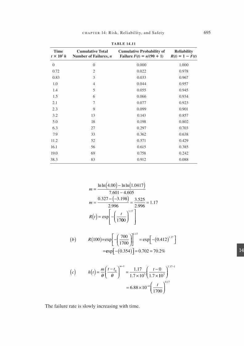
chapter 14: Risk, Rel iabil ity, and Safety 695
14
m
m
=( ) − ( )
−
=
ln ln 4.00 ln ln 1.0417
7 601 4 605
0 327
. .
. −− −( )= =
( ) = −
3 198
2 996
3 525
2 9961 17
17
.
.
.
..
R tt
exp000
1 17
.
b R( ) ( )= −
= −( )
=
100700
1700
1 17
1 17exp exp 0.412
.
.
eexp −( ) = =0 354 0 702 70 2. . . %
c h tm t t t
m
( ) ( ) =−
=
×−×
−
θ θ0
1
3
1 17
1 7 10
0
1 7
.
. . 110
6 88 101700
3
1 17 1
4
0 17
= ×
−
−
.
.
.t
The failure rate is slowly increasing with time.
TABLE 14.11
Time
t 3 10 2 h
Cumulative Total
Number of Failures, n
Cumulative Probability of
Failure F ( t ) 5 n /(90 ! 1)
Reliability
R ( t ) 5 1 F ( t )
0 0 0.000 1.000
0.72 2 0.022 0.978
0.83 3 0.033 0.967
1.0 4 0.044 0.957
1.4 5 0.055 0.945
1.5 6 0.066 0.934
2.1 7 0.077 0.923
2.3 9 0.099 0.901
3.2 13 0.143 0.857
5.0 18 0.198 0.802
6.3 27 0.297 0.703
7.9 33 0.362 0.638
11.2 52 0.571 0.429
16.1 56 0.615 0.385
19.0 69 0.758 0.242
38.3 83 0.912 0.088
die37039_ch14.indd 695 2/25/08 7:01:15 PM

696 engineering design
14
14.3.5 System Reliability
Most mechanical and electronic systems comprise a collection of components. The overall reliability of the system depends on how the individual components with their individual failure rates are arranged.
If the components are so arranged that the failure of any component causes the system to fail, it is said to be arranged in series.
R R R RA B nsystem
= × × ⋅ ⋅ ⋅× (14.28)
It is obvious that if there are many components exhibiting series reliability, the system reliability quickly becomes very low. For example, if there are 20 components each with R 5 0.99, the system reliability is 0.99 20 5 0.818. Most consumer products ex-hibit series reliability.
If we are dealing with a constant-failure-rate system,
R R R e e eA B
t t tA B A B
system= × = × =− − − +( )λ λ λ λ
and the value of l for the system is the sum of the values of l for each component.
0.10
0.20
0.30
0.40
0.50
0.60
0.700.632
0.80
0.90
0.99
0.01103
t, hours
F(t
)
102101
FIGURE 14.8
Plot of F ( t ) vs. time on Weibull
probability paper, for the data in
Table 13.11.
die37039_ch14.indd 696 2/25/08 7:01:15 PM

chapter 14: Risk, Rel iabil ity, and Safety 697
14
A much better arrangement of components is one in which it is necessary for all components in the system to fail in order for the system to fail. This is called parallel reliability.
R R R RA B nsystem
= − −( ) −( ) ⋅ ⋅ ⋅ −( )1 1 1 1 (14.29)
If we have a constant-failure-rate system,
R R R e e
A B
t tA B
system= − −( ) −( ) = − −( ) −( )− −
1 1 1 1 1 1λ λ
== + −− − − +( )e e eA B A Bt t tλ λ λ λ
Since this is not in the form e 2const , the parallel system has a variable failure rate. A system in which the components are arranged to give parallel reliability is said
to be redundant; there is more than one mechanism for the system functions to be carried out. In a system with full active redundancy, all but one component may fail before the system fails.
Other systems have partial active redundancy, in which certain components can fail without causing system failure, but more than one component must remain operat-ing to keep the system operating. A simple example would be a four-engine aircraft that can H y on two engines but would lose stability and control if only one engine were operating. This type of situation is known as an n -out-of- m unit network. At least n units must function normally for the system to succeed rather than only one unit in the parallel case and all units in the series case. The reliability of an n -out-of- m sys-tem is given by a binomial distribution, on the assumption that each of the m units is independent and identical.
Rm
iR R
n mi n
mi m i
=
−( )
=
−∑ 1 (14.30)
where m
i
m
i m i
=
−( )!
! !
E X A M P L E 14 . 7
A complex engineering design can be described by a reliability block diagram as shown
in Fig. 14.9. In subsystem A, two components must operate for the subsystem to function
successfully. Subsystem C has true parallel reliability. Calculate the reliability of each
subsystem and the overall system reliability.
Subsystem A is an n -out-of- m model for which n 5 2 and m 5 4. Using Eq. (14.30),
Ri
R RA
i i
i
=
−( ) −
=∑
41
4
2
4
4
21
4
31
4
4
6 1 2 4
2 2 3 4
2 2
−( ) +
−( ) +
− +( ) +
R R R R R
R R R R33 4
4 3 2 4 3 2
1 1
3 8 6 3 0 92 8 0 92 6 0 92 0 998
−( ) + ( )− + = ( ) − ( ) + ( ) =
R R
R R R . . . .
die37039_ch14.indd 697 2/25/08 7:01:15 PM
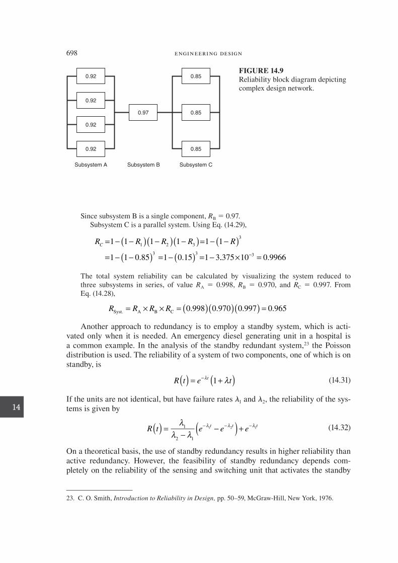
698 engineering design
14
Since subsystem B is a single component, R B 5 0.97.
Subsystem C is a parallel system. Using Eq. (14.29),
R R R R R
C= − −( ) −( ) −( )= − −( )= − −( ) = − ( ) = −
1 1 1 1 1 1
1 1 0 85 1 0 15 1 3
1 2 3
3
3 3. . .. .375 10 0 99663× =−
The total system reliability can be calculated by visualizing the system reduced to
three subsystems in series, of value R A 5 0.998, R B 5 0.970, and R C 5 0.997. From
Eq. (14.28),
R R R RSyst. A B C
= × × = ( )( )( ) =0 998 0 970 0 997 0 965. . . .
Another approach to redundancy is to employ a standby system, which is acti-vated only when it is needed. An emergency diesel generating unit in a hospital is a common example. In the analysis of the standby redundant system, 23 the Poisson distribution is used. The reliability of a system of two components, one of which is on standby, is
R t e tt( ) = +( )−λ λ1 (14.31)
If the units are not identical, but have failure rates l 1 and l 2 , the reliability of the sys-tems is given by
R t e e et t t( ) =
−−( ) +− − −λ
λ λλ λ λ1
2 1
1 2 1 (14.32)
On a theoretical basis, the use of standby redundancy results in higher reliability than active redundancy. However, the feasibility of standby redundancy depends com-pletely on the reliability of the sensing and switching unit that activates the standby
0.92
0.92
0.97
0.92
0.92
0.85
0.85
0.85
Subsystem A Subsystem B Subsystem C
FIGURE 14.9
Reliability block diagram depicting
complex design network.
23. C. O . Smith , Introduction to Reliability in Design, pp. 50–59 , McGraw-Hill, New York , 1976 .
die37039_ch14.indd 698 2/25/08 7:01:16 PM

chapter 14: Risk, Rel iabil ity, and Safety 699
14
unit. When this key factor is considered, the reliability of a standby system is little better than that of an active redundant system.
14.3.6 Maintenance and Repair
An important category of reliability problems deals with maintenance and repair of systems. If a failed component can be repaired while a redundant component has re-placed it in service, then the overall reliability of the system is improved. If compo-nents subject to wear can be replaced before they have failed, then the system reliabil-ity will be improved.
Preventive maintenance is aimed at minimizing system failure. Routine mainte-nance, such as lubricating, cleaning, and adjusting, generally does not have a major positive effect on reliability, although the absence of routine maintenance can lead to premature failure. Replacement before wearout is based on knowledge of the sta-tistical distribution of failure time; components are replaced sooner than they would normally fail. Here a small part of the useful life is traded off for increased reliability. This approach is greatly facilitated if it is possible to monitor some property of the component that indicates degradation toward an unacceptable performance.
Repairing a failed component in a series system will not improve the reliability, since the system is not operating. However, decreasing the repair time will shorten the period during which the system is out of service, and thus the maintainability and availability will be improved.
A redundant system continues to operate when a component has failed, but it may become vulnerable to shutdown unless the component is repaired and placed back in service. To consider this fact we deB ne some additional terms.
MTBF MTTF MTTR= + (14.33)
where MTBF 5 mean time between failures 5 1/l for constant failure rate. MTTF 5 mean time to fail MTTR 5 mean time to repair
If the repair rate r 5 1/MTTR, then for an active redundant system,
MTTF3
=+λ
λr
2 2 (14.34)
As an example of the importance of repair, let r 5 6 h 21 and l 5 10 25 per h. With repair, the MTTF 5 3 3 10 10 h, but without repair it is 1.5 3 10 5 h.
Maintainability is the probability that a component or system that has failed will be restored to service within a given time. The MTTF and failure rate are measures of reliability, but the MTTR and repair rate are measures of maintainability.
M t e ert t( ) = − = −− −1 1 /MTTR (14.35)
where M ( t ) 5 maintainability r 5 repair rate t 5 permissible time to carry out the required repair
die37039_ch14.indd 699 2/25/08 7:01:16 PM
700 engineering design
14
It is important to try to predict maintainability during the design of an engineer-ing system. 24 The components of maintainability include (1) the time required to de-termine that a failure has occurred and to diagnose the necessary repair action, (2) the time to carry out the necessary repair action, and (3) the time required to check out the unit to establish that the repair has been effective and the system is operational. An important design decision is to establish what constitutes the least repairable as-sembly, that is, the unit of the equipment beyond which diagnosis is not continued but the assembly simply is replaced. An important design trade-off is between MTTR and cost. If MTTR is set too short for the labor hours to carry out the repair, then a large maintenance crew will be required at an increased cost.
Availability is the concept that combines both reliability and maintainability; it is the proportion of time the system is working “on line” to the total time, when that is determined over a long working period.
Availability total on-line time
total on-line time total =
+ ddowntime
total on-line time
total on-line time no. of fail=
+ uures MTTR
total on-line time
total on-line time t
×( )
=+ ×λ ootal on-line time MTTR
MTTR
×( )
=+
1
1 λ (14.36)
If MTTF 5 1/l, then
AvailabilityMTTF
MTTF MTTR=
+ (14.37)
14.3.7 Further Topics
In Sec. 14.3 we have mainly covered situations dealing with continuous variables that can take on any value over a considerable range of data. Also, we have not covered in any detail how to examine a mass of data to determine its characteristics of central tendency and variability, or how to determine what frequency distribution best de-scribes the data. Nor have we discussed how to determine with conB dence whether two experimentally determined values are statistically signiB cant from each other. Moreover, we have given scant attention to the statistics of discrete variables other than to mention the binomial and Poisson distributions in passing. For these and
24. B. S . Blanchard , Logistics Engineering and Management, 2d ed., Prentice Hall, Englewood Cliffs,
NJ , 1981 ; C. E . Cunningham and W . Cox , Applied Maintainability Engineering, John Wiley & Sons,
New York , 1972 ; A. K. S . Jardine , Maintenance, Replacement and Reliability, John Wiley & Sons, New
York , 1973 .
die37039_ch14.indd 700 2/25/08 7:01:16 PM
chapter 14: Risk, Rel iabil ity, and Safety 701
14
other topics of engineering we suggest reading beginning texts 25 or a formal course in statistics.
We have just begun to scratch the surface of such a dynamic and rich subject as reliability engineering. Models for realistic situations where reliability varies with time are important. Also, there are models for censored or truncated frequency distri-butions in which a life test is terminated after a speciB ed number of failures have oc-curred. Another extension is models for the case where each element in a system fails by two mutually exclusive failure modes, and the further reB nement where failure is by a common cause. A common cause failure is one where a single event can lead to multiple failures. Often such failure results from the location of a component, as when an aircraft turbine disk shatters and the H ying pieces break several independent hy-draulic control systems of the airplane. Additional complexity yet realism arises when the repairability condition is added to the above reliability models. These topics are beyond the scope of this book. The interested reader is referred to the references in the Bibliography at the end of this chapter.
14.4 DESIGN FOR RELIABILITY
The design strategy used to ensure reliability can fall between two broad extremes. The fail-safe approach is to identify the weak spot in the system or component and provide some way to monitor that weakness. When the weak link fails, it is replaced, just as the fuse in a household electrical system is replaced. At the other extreme is what can be termed “the one-horse shay” approach. The objective is to design all com-ponents to have equal life so the system will fall apart at the end of its useful lifetime just as the legendary one-horse shay did. Frequently an absolute worst-case approach is used; in it the worst combination of parameters is identiB ed and the design is based on the premise that all can go wrong at the same time. This is a very conservative ap-proach, and it often leads to overdesign.
Two major areas of engineering activity determine the reliability of an engineer-ing system. First, provision for reliability must be established during the design con-cept stage, carried through the detailed design development, and maintained during the many steps in manufacture. Once the system becomes operational, it is imperative that provision be made for its continued maintenance during its service. 26
The steps in building reliability into a design are shown in Fig. 14.10. The process starts at the beginning of conceptual design by clearly laying out the criteria for the success of the design, estimating the required reliability, the duty cycle, and carefully considering all of the factors that make up the service environment. In the conB guration
25. W . Navidi , Statistics for Engineers and Scientists, 2d ed., McGraw-Hill, New York , 2008 ; G. P . Box ,
W. G . Hunter , and J. S . Hunter , Statistics for Experimenters, 2d ed., John Wiley & Sons, New York , 2005 .
26. H. P . Bloch and F. K . Gleitner , An Introduction to Machinery Reliability Assessment, 2d ed., Gulf
Publishing Co., Houston, TX , 1994 ; H. P . Bloch , Improving Machinery Reliability, 3d ed., Gulf Publish-
ing Co. , 1998 ; H. P . Bloch , and F. K . Geitner , Machinery Failure Analysis and Troubleshooting, Gulf
Publishing Co., Houston, TX , 1997 .
die37039_ch14.indd 701 2/25/08 7:01:17 PM

702 engineering design
14
step of embodiment design the physical arrangement of components can critically affect reliability. In laying out functional block diagrams, consider those areas that strongly inH uence reliability, and prepare a list of parts in each block. This is the place to consider various redundancies and to be sure that physical arrangement al-lows good access for maintenance. In the parametric step of embodiment design, select components with high reliability. Build and test both computer and physical prototypes. These should be subjected to the widest range of environmental condi-tions. Establish failure modes and estimate the system and subsystem MTBF. Detail design is the place for the B nal revision of speciB cations, for building and testing the preproduction prototype, and the preparation of the B nal production drawings. Once the design is released to the production organization the design organization is not B nished with it. Production models are given further environmental tests, and these help establish the quality assurance program (see Sec. 15.2) and the maintenance schedules. When the product is put into service with customers, there is a steady feed-back concerning B eld failures and MTBFs that helps in redesign efforts and follow-on products.
FIGURE 14.10
Reliability activities throughout design, production, and service.
Design Stage Design Activity
Conceptual design Problem definition:
Estimate reliability requirement
Determine likely service environment
Embodiment design Configuration design:
Investigate redundancy
Provide accessibility for maintenance
Parametric design:
Select highly reliable components
Build and test physical and computer prototypes
Full environment tests
Establish failure modes/FMEA
Estimate MTBF
User trials/modification
Detail design Produce & test preproduction prototype
Final estimate of reliablity
Production Production models:
Further environmental tests
Establish quality assurance program
Service Deliver to customer:
Feedback field failures and MTBFs to designers
Repair and replace
Retirement from service
die37039_ch14.indd 702 2/25/08 7:01:17 PM
chapter 14: Risk, Rel iabil ity, and Safety 703
14
14.4.1 Causes of Unreliability
The malfunctions that an engineering system can experience can be classiB ed into B ve general categories. 27
Design mistakes: Among the common design errors are failure to include all im-portant operating factors, incomplete information on loads and environmental con-ditions, erroneous calculations, and poor selection of materials. Manufacturing defects: Although the design may be free from error, defects intro-duced at some stage in manufacturing may degrade it. Some common examples are (1) poor surface B nish or sharp edges (burrs) that lead to fatigue cracks and (2) decarburization or quench cracks in heat-treated steel. Elimination of defects in manufacturing is a key responsibility of the manufacturing engineering staff, but a strong relationship with the R&D function may be required to achieve it. Manufacturing errors produced by the production work force are due to such fac-tors as lack of proper instructions or speciB cations, insufB cient supervision, poor working environment, unrealistic production quota, inadequate training, and poor motivation. Maintenance: Most engineering systems are designed on the assumption they will receive adequate maintenance at speciB ed periods. When maintenance is neglected or is improperly performed, service life will suffer. Since many consumer products do not receive proper maintenance by their owners, a good design strategy is to design products that do not require maintenance. Exceeding design limits: If the operator exceeds the limits of temperature, speed, or another variable for which it was designed, the equipment is likely to fail. Environmental factors: Subjecting equipment to environmental conditions for which it was not designed, such as rain, high humidity, and ice, usually greatly shortens its service life.
14.4.2 Minimizing Failure
A variety of methods are used in engineering design practice to improve reliability. We generally aim at a probability of failure of P f , 10 26 for structural applications and 10 24 , P f , 10 23 for unstressed applications.
Margin of Safety
We saw in Sec. 14.2.3 that variability in the strength properties of materials and in loading conditions (stress) leads to a situation in which the overlapping statistical distributions can result in failures. The variability in strength of materials has a major impact on the probability of failure, so failure can be reduced with no change in the mean value if the variability of the strength can be reduced.
1.
2.
3.
4.
5.
27. W . Hammer , Product Safety Management and Engineering, Chap. 8, Prentice Hall, Englewood
Cliffs, NJ , 1980 .
die37039_ch14.indd 703 2/25/08 7:01:17 PM

704 engineering design
14
Derating
The analogy to using a factor of safety in structural design is derating electrical, electronic, and mechanical equipment. The reliability of such equipment is increased if the maximum operating conditions (power, temperature, etc.) are derated below their nameplate values. As the load factor of equipment is reduced, so is the failure rate. Conversely, when equipment is operated in excess of rated conditions, failure will ensue rapidly.
Redundancy
One of the most effective ways to increase reliability is with redundancy. In paral-lel redundant designs the same system functions are performed at the same time by two or more components even though the combined outputs are not required. The ex-istence of parallel paths may result in load sharing so that each component is derated and has its life increased by a longer-than-normal time.
Another method of increasing redundancy is to have inoperative or idling standby units that cut in and take over when an operating unit fails. The standby unit wears out much more slowly than the operating unit does. Therefore, the operating strategy of-ten is to alternate units between full-load and standby service. The standby unit must be provided with sensors to detect the failure and switching gear to place it in service. The sensor and/or switching units frequently are the weak link in a standby redundant system.
Durability
The material selection and design details should be performed with the objective of producing a system that is resistant to degradation from such factors as corrosion, erosion, foreign object damage, fatigue, and wear. 28 This usually requires the decision to spend more money on high-performance materials so as to increase service life and reduce maintenance costs. Life cycle costing is the technique used to justify this type of decision.
Damage Tolerance
Crack detection and propagation have taken on great importance since the devel-opment of the fracture mechanics approach to design (Sec. 12.2). A damage-tolerant material or structure is one in which a crack, when it occurs, will be detected soon enough after its occurrence so that the probability of encountering loads in excess of the residual strength is very remote. Figure 14.11 illustrates some of the concepts of damage tolerance. The initial population of very small H aws inherent in the material is shown at the far left. These are small cracks, inclusions, porosity, surface pits, and scratches. If they are less than a 1 , they will not grow appreciably in service. Additional defects will be introduced by manufacturing processes. Those larger than a 2 will be detected by inspection and eliminated as scrapped parts. However, some cracks will be present in the components put into service, and they will grow to a size a 3 that can be detected by the nondestructive evaluation (NDE) techniques that can be used in
28. A. L . Smith (ed.), “Reliability of Engineering Materials,” Butterworth, London , 1984 .
die37039_ch14.indd 704 2/25/08 7:01:18 PM

chapter 14: Risk, Rel iabil ity, and Safety 705
14
service. The allowable design stresses must be so selected that the number of H aws of size a 3 or greater will be small. Moreover, the material should be damage-tolerant so that propagation to the critical crack size a cr is slow.
In conventional fracture mechanics analysis (Sec. 12.2), the critical crack size is set at the largest crack size that might be undetected by the NDE technique used in service. The value of fracture toughness of the material is taken as the minimum rea-sonable value. This is a safe but overly conservative approach. These worst-case as-sumptions can be relaxed and the analysis based on more realistic conditions by using probabilistic fracture mechanics (PFM). 29
Ease of Inspection
The importance of detecting cracks should be apparent from Fig. 14.11. Ideally it should be possible to employ visual methods of crack detection, but special design features may have to be provided in order to do so. In critically stressed structures, special features to permit reliable NDE by ultrasonics or eddy current techniques may be required. If the structure is not capable of ready inspection, then the stress level must be lowered until the initial crack cannot grow to a critical size during the life of the structure. For that situation the inspection costs will be low but the structure will carry a weight penalty because of the low stress level.
Simplicity
SimpliB cation of components and assemblies reduces the chance for error and increases the reliability. The components that can be adjusted by operation or mainte-nance personnel should be restricted to the absolute minimum. The simpler the equip-ment needed to meet the performance requirements the better the design.
a1 a2 a3 acr
Nu
mb
er
of
cra
cks o
r d
efe
cts
Defects inherent
in material
Defect size
Defects introduced
by manufacturingDefects introduced
into service
FIGURE 14.11
Distribution of defects in engineering components.
29. H. R . Millurter and P. H . Wirsching , “Analysis Methods for Probabilistic Life Assessment,” ASM
Handbook, Vol. 11, pp. 250–68 , ASM International, Materials Park, OH , 2002 .
die37039_ch14.indd 705 2/25/08 7:01:18 PM

706 engineering design
14
SpeciS city
The greater the degree of speciB city, the greater the inherent reliability of de-sign. Whenever possible, be speciB c with regard to material characteristics, sources of supply, tolerances and characteristics of the manufacturing process, tests required for qualiB cation of materials and components, and procedures for installation, main-tenance, and use. Specifying standard items increases reliability. It usually means that the materials and components have a history of use so that their reliability is known. Also, replacement items will be readily available. When it is necessary to use a com-ponent with a high failure rate, the design should especially provide for the easy re-placement of that component.
14.4.3 Sources of Reliability Data
Data on the reliability of a product clearly is highly proprietary to its manufacturer. However, the U.S. defense and space programs have created a strong interest in reliabil-ity, and this has resulted in the compilation of a large amount of data on failure rates and failure modes. The Reliability Information Analysis Center (RIAC) 30 , sponsored by the DOD Defense Information Analysis Center, has for many years collected fail-ure data on electronic components. Extensive reliability data on electronic components is available online, for a fee, in 217 Plus, the successor to MIL-HDBK-217. Reliability data on nonelectronic components is available on compact disk NPRD-95. Informa-tion on European sources of reliability data can be found in the book by Moss. 31 Ap-pendix G of this book contains 20 pages of tables on failure rates. Data and failure rate l for a wide selection of mechanical components is given by Fisher and Fisher. 32
14.4.4 Cost of Reliability
Reliability costs money, but the cost nearly always is less than the cost of unreliability. The cost of reliability comes from the extra costs associated with designing and pro-ducing more reliable components, testing for reliability, and training and maintaining a reliability organization. Figure 14.12 shows the cost to a manufacturer of increasing the reliability of a product. The costs of design and manufacture increase with product reliability. Moreover, the slope of the curve increases, and each incremental increase in reliability becomes harder to achieve. The costs of the product after delivery to the customer, chieH y warranty or replacement costs and reputation of the supplier, de-crease with increasing reliability. The summation of these two curves produces the to-tal cost curve, which has a minimum at an optimum level of reliability. 33 Other types of analyses establish the optimum schedule for part replacement to minimize cost. 34
30 . http://quanterion.com/RIAC/index.asp
31. T. R . Moss , The Reliability Data Handbook, ASME Press, New York , 2005 .
32. F. E . Fisher and J. R. Fisher , Probabilistic Applications in Mechanical Design, Appendix D, Marcel
Dekker, New York , 2000 .
33. R. G . Fenton , Trans. ASME, Ser. B, J. Eng. Ind. , vol. 98, pp. 1066–68 , 1976 .
34. N. W . Nelson and K . Hayashi , ibid. , vol. 96, pp. 311–16 , 1974 .
die37039_ch14.indd 706 2/25/08 7:01:18 PM

chapter 14: Risk, Rel iabil ity, and Safety 707
14
14.5 FAILURE MODE AND EFFECTS ANALYSIS (FMEA)
Failure mode and effects analysis (FMEA) is a team-based methodology for identify-ing potential problems with new or existing designs. 35 It is one of the most frequently used hazard-analysis tools. FMEA identiB es the mode of failure of every component in a system and determines the effect on the system of each potential failure. By fail-ure we mean inability to meet a customer’s requirements as opposed to actual cata-strophic material breakage or failure.
Thus, a failure mode is any way that a part could fail to perform its required function. For example, a cable used to lift I-beams could fray from wear, kink from misuse, or actually fracture from excessive load. Note that either fraying or kinking could lead to fracture, but fracture might occur without these events if a design error incorrectly estimated either the strength of the cable or the load it needed to support. Failure modes are discussed in more detail in Sec. 14.6.
There are many variations in detailed FMEA methodology, but they are all aimed at accomplishing three things: (1) predicting what failures could occur; (2) predict-ing the effect of the failure on the functioning of the system; and (3) establishing steps that might be taken to prevent the failure, or its effect on the function. FMEA is useful in identifying critical areas of the design that need redundant components and improved reliability. FMEA is a bottom-up process that starts with the required functions, identiB es the components to provide the functions, and for each component, lists all possible modes of failure.
Co
st
Total cost
Cost of design
and manufactureCosts after delivery
Reliability
FIGURE 14.12
InH uence of reliability on cost.
35. Failure Mode and Effects Analysis Handbook, Ford Motor Company , 1988 ; D. H . Stamatis , Fail-
ure Mode and Effects Analysis: FMEA from Theory to Execution, ASQ Quality Press, Milwaukee,
WI , 1995 ; P . Palady , Failure Modes & Effects Analysis, Practical Applications, Ann Arbor, MI , 1998 ;
MIL-STD-1629.
die37039_ch14.indd 707 2/25/08 7:01:19 PM

708 engineering design
14
Three factors are considered in developing a FMEA.
The severity of a failure. Table 14.12 gives the scale for rating severity. Many or-ganizations require that potential failures with a 9 or 10 rating require immediate redesign. The probability of occurrence of the failure. Table 14.13 gives a scale for prob-ability of occurrence. The probabilities given are very approximate and depend on the nature of the failure, the robustness of the design, and the level of quality developed in manufacturing. The likelihood of detecting the failure in either design or manufacturing, before the product is used by the customer. Table 14.14 gives the scale for detection. Clearly, the rating for this factor depends on the quality review systems in place in the organization.
1.
2.
3.
TABLE 14.12
Rating for Severity of Failure
Rating Severity Description
1 The effect is not noticed by the customer
2 Very slight effect noticed by customer; does not annoy or inconvenience customer
3 Slight effect that causes customers annoyance, but they do not seek service
4 Slight effect, customer may return product for service
5 Moderate effect, customer requires immediate service
6 SigniB cant effect, causes customer dissatisfaction; may violate a regulation or design code.
7 Major effect, system may not be operable; elicits customer complaint; may cause injury
8 Extreme effect, system is inoperable and a safety problem. May cause severe injury.
9 Critical effect, complete system shutdown; safety risk
10 Hazardous; failure occurs without warning; life-threatening
TABLE 14.13
Rating for Occurrence of Failure
Rating Approx. Probability of Failure Description of Occurrence
1 < 1 3 10 –6 Extremely remote
2 1 3 10 –5 Remote, very unlikely
3 1 3 10 –5 Very slight chance of occurrence
4 4 3 10 –4 Slight chance of occurrence
5 2 3 10 –3 Occasional occurrence
6 1 3 10 –2 Moderate occurrence
7 4 3 10 –2 Frequent occurrence
8 0.20 High occurrence
9 0.33 Very high occurrence
10 > 0.50 Extremely high occurrence
die37039_ch14.indd 708 2/25/08 7:01:19 PM

chapter 14: Risk, Rel iabil ity, and Safety 709
14
Usual practice is to combine the rating for the three factors into a risk priority number (RPN).
RPN severity of failure occurrence of f= ( ) × aailure detection rating( ) × ( ) (14.38)
Values of RPN can vary from a maximum of 1000, the greatest risk, to a minimum of 1. Numbers derived from Eq. (14.38) are often used to select the “vital few” problems to work on. This can be done by setting a threshold limit, for example, RPN 5 200, and working on all potential failures above this limit. Another approach is to arrange the RPN values in a Pareto plot and give attention to those potential failures with the highest ratings. The next paragraph suggests an alternative approach.
Decisions on how to use the information provided from the FMEA should not be blindly based on the RPN values. Consider the results of a FMEA analysis shown in Table 14.15.
Compare failure modes A and B. A has nearly four times the RPN of B, yet B has a severity of failure that would cause safety risk and complete system shutdown. Fail-ure by A would cause only a slight effect on product performance. It achieves its high RPN value because it is not possible to detect the defect that is causing the failure. Certainly failure B is more critical than A and should be given prompt attention for design of the product. Failure mode C has over 2 times the RPN of B, but because the
TABLE 14.14
Rating for Detection of Failure
Rating Description of Detection
1 Almost certain to detect
2 Very high chance of detection
3 High chance of detection
4 Moderately high chance of detection
5 Medium chance of detection
6 Low chance of detection
7 Slight chance of detection
8 Remote chance of detection
9 Very remote chance of detection
10 No chance of detection; no inspection
TABLE 14.15
Results of a FMEA Analysis
Failure Mode Severity Occurrence Detection RPN
A 3 4 10 120
B 9 4 1 36
C 3 9 3 81
die37039_ch14.indd 709 2/25/08 7:01:19 PM

710 engineering design
14
severity of the failure is low it should be given lower priority than B even though the occurrence of failure is high.
A rational way to interpret the results of FMEA analysis has been given by Harpster, 36 Fig. 14.13. Often product speciB cations include a requirement that action should be taken if the RPN value exceeds some number like 100 or 200. It may not be rational to require a design change if the reason for the high RPN is due to a very hard-to-detect defect or if detectability scores high because no inspection process is in use. Using a plot such as Fig. 14.13 gives better guidance on which design details (failure modes) require remedial action than simply basing all decisions on the RPN value.
14.5.1 Making a FMEA Analysis
The development of a FMEA is best done as a team effort that employs many of the problem-solving tools presented in Sec. 4.7. FMEA can be done on a design, a manu-facturing process, or a service. While there is no well-deB ned format, as there is for QFD, a FMEA is usually developed in a spreadsheet format. 37 First you must clearly identify the system or subassembly that you are investigating. Then the following steps are performed and the results recorded in the spreadsheet, Example 14.8.
The design is reviewed to determine the interrelations of assemblies and the inter-relations of the components of each subassembly. Identify how each component might fail to perform its required function. A complete list of the components in each assembly and the function of each component is prepared. For each func-
1.
36. R. A . Harpster . Quality Digest, pp. 40–42 , June 1999 .
37 . FMEA software is available to aid in the process. Two examples are FailMode®, from Item Software,
and FMEAplus®, developed by Ford Motor Co. and available from Adistra Corp. or the Society of Auto-
motive Engineers.
10
9
8
7
6
5
4Se
ve
rity
3
2
1
1 2 3 4 5
Occurrence
A
C
B
Warranty
issues
Legal or code issues
6 7 8 9 10
FIGURE 14.13
A rational way to interpret
FMEA results.
die37039_ch14.indd 710 2/25/08 7:01:20 PM

chapter 14: Risk, Rel iabil ity, and Safety 711
14
tion ask, “What if this function fails to take place?” To further sharpen the point ask: ● What if the function fails to occur at the right time? ● What if the function fails to occur in the proper sequence? ● What if this function fails to occur completely? Now look more broadly, and ask what are the consequences to the system of each failure identiB ed in step 1. It may be difB cult to answer this question in systems for which the subsystems are not independent. A frequent cause of hazardous failures is that an apparently innocuous failure in one subsystem overloads an-other subsystem in an unexpected way. For each of the functions, list the potential failure modes (see Sec. 14.6). There are likely to be several potential failure modes associated with each of the functions. For each of the failure modes identiB ed in step 3, describe the consequences or effects of the failure. First list the local effect on the particular component; then extend the effects analysis to the entire subassembly and to the total system. Using the severity of failure table (Table 14.12), enter the numerical value. This is best done as a team using consensus decision methods. Identify the possible causes of the failure mode. Try to determine the root cause by using a why-why diagram and interrelationship digraph. Using the occurrence of failure table (Table 14.13), enter a value for the occur-rence of the cause of each failure. Determine how the potential failure will be detected. This might be a design checklist, a speciB c design calculation, a visual quality inspection, or a nonde-structive inspection. Using Table 14.14, enter a rating that reH ects the ability to detect the cause of failure identiB ed in step 8. Calculate the risk priority number (RPN) from Eq. (14.38). Those potential fail-ures with the highest RPN values will be given priority action. In making deci-sions about where to deploy the resources, also consider Fig. 14.13. For each potential failure, determine the corrective action to remove a potential design, manufacturing, or operational failure. One of the actions might be “no action required.” Assign ownership for the removal of each potential failure.
E X A M P L E 14 . 8
RiH e bolts are made by a powder forging process in which steel preforms of the riH e bolt;
are made by cold pressing and sintering, followed by hot forging to the required shape
and dimensions. The completed chart for the FMEA is given below. Note that the analysis
rates the part design and process as it performs in service, and then recommends design
or process changes that are expected to improve the RPN of the design.
When the bolt in a riH e fractures, it is the most severe type of failure since the prod-
uct no longer functions, but of more importance, someone’s life is in great danger. The
corrective action is to scan all B nished parts with 3-D x-ray tomography, the most precise
nondestructive inspection method, to reject any parts with B ne cracks in the interior of the
metal part. This is an expensive step taken while the powder forging process is studied in
detail to identify the source of the B ne cracks. If these cannot be eliminated, then another
2.
3.
4.
5.
6.
7.
8.
9.
10.
11.
die37039_ch14.indd 711 2/25/08 7:01:20 PM

712 engineering design
14
Failure Modes and Effect Analysis Prepared by: Sheet No. of
Product name: Part name: Ria e bolt Primary design responsibility:
Product code: Part no.: Design deadline:
1 2 3 4 5 6 7 8 9 10 11 12 13 14
Function Failure
mode
Effects
of failure
Causes
of failure
Detection S O D RPN Recommended
corrective
action
S O D RPN
1. Cham-
bers and
B res the
round.
Brittle
fracture
Destroys
riH e.
Injures
people.
Internal
B ne
cracks
Dye
penetrant
10 4 8 320 Scan all
parts with
x-ray
tomography.
10 1 2 20
2. Seals
against gas
blowback.
3. Extracts
cartridge
case.
Jamming
after B ring
4 clips in
succession.
RiH e will
not B re
another
round.
CTQ
dimen-
sions out
of spec.
Dimensions
checked
with
gages.
8 6 3 144 Rework toler-
ances to incl.
thermal expan-
sion. Start SPC.
3 4 2 24
manufacturing process would be used to make the part. Note that the severity of the event
is not changed by the corrective action, but the occurrence is set at one chance in a mil-
lion because of the consequences of failure of this part.
The second failure found in the riH e is jamming of the bolt in the chamber. This makes
the riH e inoperable, but is less life threatening than a failure by fracture. Examination of
the design notebooks showed that thermal expansion of the bolt due to heating produced
by extensive rapid B re was not taken into account when setting the tolerances for the
original design. When this is done, and statistical process control (SPC) is initiated
for the critical-to-quality dimensions, it is expected that this will eliminate failure by
jamming.
FMEA is a powerful design tool, but it can be tedious and time consuming. It re-quires top-level corporate support to make sure it is used routinely. However, FMEA reduces total life cycle cost by avoiding cost due to warranty problems, service calls, customer dissatisfaction, product recalls, and damaged reputation.
14.6 DEFECTS AND FAILURE MODES
Failures of engineering designs and systems are a result of deB ciencies in four broad categories.
Hardware failure—failure of a component to function as designed. Software failure—failure of the computer software to function as designed. Human failure—failure of human operators to follow instructions or respond ad-equately to emergency situations.
●
●
●
die37039_ch14.indd 712 2/25/08 7:01:20 PM

chapter 14: Risk, Rel iabil ity, and Safety 713
14
Organizational failure—failure of the organization to properly support the system. Examples might be overlooking defective components, slowness to bring corrective action, or ignoring bad news.
14.6.1 Causes of Hardware Failure
Failures are caused by design errors or deB ciencies in one or more of the following categories:
Design deB ciencies Failure to adequately consider the effect of notches Inadequate knowledge of service loads and environment DifB culty of stress analysis in complex parts and loadings
DeB ciency in selection of material Poor match between service conditions and selection criteria Inadequate data on material Too much emphasis given to cost and not enough to quality
Imperfection in material due to manufacturing Improper testing or inspection Overload and other abuses in service Inadequate maintenance and repair Environmental factors
Conditions beyond those allowed for in design Deterioration of properties with time of exposure to environment
DeB ciencies in the design process, or defects in the material or its processing, can be classiB ed in the following ways: At the lowest level is a lack of conformance to a stated speciB cation. An example would be a dimension “out of spec” or a strength property below speciB cation. Next in severity is a lack of satisfaction by the customer or user. This may be caused by a critical performance characteristic set at an improper value, or it may be a system problem caused by rapid deterioration. The ultimate defect is one that causes failure of the product. Failure may be an actual fracture or disruption of physical continuity of the part, or failure may be inability of the part to function properly.
14.6.2 Failure Modes
The speciB c modes of failure of engineering components can usually be grouped into four general classes:
Excessive elastic deformation Excessive plastic deformation Fracture Loss of required part geometry through corrosion or wear
The most common failure modes are listed in Table 14.16. Some of these failure modes are directly related to a standard mechanical property test, but most are more
●
1.
2.
3.4.5.6.7.
1.2.3.4.
die37039_ch14.indd 713 2/25/08 7:01:21 PM

714 engineering design
14 TABLE 14.17
Examples of Failure Modes in Components
Component Failure Mode Possible Cause
Battery Discharged Extended use
Check valve Stuck closed Corrosion
Piping Sagging pipes Designed inadequate supports
Valve Leaks Faulty packing
Lubricant No H ow Clogged by debris/no B lter
Bolt Threads stripped Excessive tightening torque
TABLE 14.16
Failure Modes for Mechanical Components
1. Elastic deformation d. Surface fatigue wear
2. Yielding e. Deformation wear
3. Brinelling f. Impact wear
4. Ductile failure g. Fretting wear
5. Brittle fracture 9. Impact
6. Fatigue a. Impact fracture
a. High-cycle fatigue b. Impact deformation
b. Low-cycle fatigue c. Impact wear
c. Thermal fatigue d. Impact fretting
d. Surface fatigue e. Impact fatigue
e. Impact fatigue 10. Fretting
f. Corrosion fatigue a. Fretting fatigue
g. Fretting fatigue b. Fretting wear
7. Corrosion c. Fretting corrosion
a. Direct chemical attack 11. Galling and seizure
b. Galvanic corrosion 12. Scoring
c. Crevice corrosion 13. Creep
d. Pitting corrosion 14. Stress rupture
e. Intergranular corrosion 15. Thermal shock
f. Selective leaching 16. Thermal relaxation
g. Erosion-corrosion 17. Combined creep and fatigue
h. Cavitation 18. Buckling
i. Hydrogen damage 19. Creep buckling
j. Biological corrosion 20. Oxidation
k. Stress corrosion 21. Radiation damage
8. Wear 22. Bonding failure
a. Adhesive wear 23. Delamination
b. Abrasive wear 24. Erosion
c. Corrosive wear
die37039_ch14.indd 714 2/25/08 7:01:21 PM

chapter 14: Risk, Rel iabil ity, and Safety 715
14
complex, and failure prediction requires using a combination of two or more proper-ties. However, not all failures are related to material behavior. Table 14.17 gives some failures modes for common engineering components.
14.6.3 Importance of Failure
It is a human tendency to be reluctant to talk about failure or to publish much infor-mation about failures. Spectacular system failures, like the Tacoma Narrows bridge or the O-ring seal on the space shuttle Challenger solid rocket booster, have caught the public’s attention, but most failures go unheralded. 38 This is a shame, because much learning in engineering occurs by studying failures. Simulated service test-ing and proof-testing of preproduction prototypes are important steps at arriving at a successful product. While the literature on engineering failures is not extensive, there are several useful books on the subject. 39 For information on conducting failure analy-sis 40 see Techniques for Failure Analysis at www.mhhe.com/dieter.
14.7 DESIGN FOR SAFETY
Safety may well be the paramount issue in product design. 41 Normally we take safety for granted, but the recall of an unsafe product can be very costly in terms of product liability suits, replaced product, or tarnished reputation. The product must be safe to manufacture, to use, and to dispose of after use. 42 Also, a serious accident in which a life is lost can be very traumatic to the person responsible, and possibly career ending to the responsible engineer.
A safe product is one that does not cause injury or property loss. Also included under safety is injury to the environment. Achieving safety is no accident. It comes from a conscious focus on safety during design, and in knowing and following some basic rules. There are three aspects to design for safety:
Make the product safe, that is, design all hazards out of the product. If it is not possible to make the product inherently safe, then design in protective devices like guards, automatic cutoff switches, and pressure-relief valves, to miti-gate the hazard.
1.2.
38 . See http://www.matscienc.sunvsb.edu/disaster/
39. Case Histories in Failure Analysis, ASM International, Materials Park, OH , 1979 ; H . Petroski ,
Success through Failure: the Paradox of Design, Princeton University Press, Princeton , NJ, 2006 ;
V . Ramachandran , et al., Failure Analysis of Engineering Structures: Methodology and Case Histo-
ries, ASM International, Materials Park, OH , 2005 ; Microelectronics Failure Analysis Desk Reference ,
5 th ed., ASM International, Materials Park, OH , 2004 .
41. C. O . Smith , “Safety in Design,” ASM Handbook, Vol. 20, pp. 139–45 , ASM International, Materials
Park, OH , 1997 .
42 . For a comprehensive safety website see http://www.safetyline.net.
40. Extensive information on conducting a failure analysis can be found in ASM Handbook, Vol 11:
Failure Analysis and Prevention, 2002, pp. 315–556.
die37039_ch14.indd 715 2/25/08 7:01:21 PM

716 engineering design
14
If step 2 cannot remove all hazards, then warn the user of the product with appro-priate warnings like labels, H ashing lights, and loud sounds.
A fail-safe design seeks to ensure that a failure will either not affect the product or change it to a state in which no injury or damage will occur. There are three vari-ants of fail-safe designs.
Fail-passive design. When a failure occurs, the system is reduced to its lowest-energy state, and the product will not operate until corrective action is taken. A circuit breaker is an example of a fail-passive device.
Fail-active design. When failure occurs, the system remains energized and in a safe operating mode. A redundant system kept on standby is an example.
Fail-operational design. The design is such that the device continues to provide its critical function even though a part has failed. A valve that is designed so that it will remain in the open position if it fails is an example.
14.7.1 Potential Dangers
We list here some of the general categories of safety hazards that need to be consid-ered in design.
Acceleration/deceleration—falling objects, whiplash, impact damage Chemical contamination—human exposure or material degradation Electrical—shock, burns, surges, electromagnetic radiation, power outage Environment—fog, humidity, lightning, sleet, temperature extremes, wind Ergonomic—fatigue, faulty labeling, inaccessibility, inadequate controls Explosions—dust, explosive liquids, gases, vapors, B nely powdered materials Fire—combustible material, fuel and oxidizer under pressure, ignition source Human factors—failure to follow instructions, operator error Leaks or spills Life cycle factors—frequent startup and shutdown, poor maintenance Materials—corrosion, weathering, breakdown of lubrication Mechanical—fracture, misalignment, sharp edges, stability, vibrations Physiological—carcinogens, human fatigue, irritants, noise, pathogens Pressure/vacuum—dynamic loading, implosion, vessel rupture, pipe whip Radiation—ionizing (alpha, beta, gamma, x-ray), laser, microwave, thermal Structural—aerodynamic or acoustic loads, cracks, stress concentrations Temperature—changes in material properties, burns, H ammability, volatility
Product hazards are often controlled by government regulation. The U.S. Con-sumer Product Safety Commission is charged with this responsibility. 43 Products de-
3.
●
●
●
43 . See the CPSC website, www.cpsc.gov.
die37039_ch14.indd 716 2/25/08 7:01:22 PM

chapter 14: Risk, Rel iabil ity, and Safety 717
14
signed for use by children are held to much higher safety standards than products intended to be used by adults. The designer must also be cognizant that in addition to providing a safe product for the customer, it must be safe to manufacture, sell, install, and service.
In our society, products that cause harm invariably result in lawsuits for dam-ages under the product liability laws. Design engineers must understand the conse-quences of these laws and how they must practice to minimize safety issues and the threat of litigation. This topic is covered in Chap. 17, which is available at www.mhhe.com/dieter.
14.7.2 Guidelines for Design for Safety 44
Recognize and identify the actual or potential hazards, and then design the prod-uct so they will not affect its functioning.
Thoroughly test prototypes of the product to reveal any hazards overlooked in the initial design.
Design the product so it is easier to use safely than unsafely. If B eld experience turns up a safety problem, determine the root cause and rede-sign to eliminate the hazard.
Realize that humans will do foolish things, and allow for it in your design. More product safety problems arise from improper product use than from product de-fects. A user-friendly product is usually a safe product.
There is a close correspondence between good ergonomic design and a safe de-sign. For example: ● Arrange the controls so that the operator does not have to move to manipulate
them. ● Make sure that B ngers cannot be pinched by levers or other features. ● Avoid sharp edges and corners. ● Point-of-operation guards should not interfere with the operator’s movement. ● Products that require heavy or prolonged use should be designed to avoid cu-
mulative trauma disorders like carpal tunnel syndrome. This means avoiding awkward positions of the hand, wrist, and arm and avoiding repetitive motions and vibration.
7. Minimize the use of H ammable materials, including packaging materials. 8. Paint and other surface B nishing materials should be chosen to comply with
EPA and OSHA regulations for toxicity to the user and for safety when they are burned, recycled, or discarded.
9. Think about the need for repair, service, or maintenance. Provide adequate ac-cess without pinch or puncture hazards to the repairer.
10. Electrical products should be properly grounded to prevent shock. Provide elec-trical interlocks so that high-voltage circuits will not be energized unless a guard is in the proper position.
1.
2.
3.4.
5.
6.
44. C. O . Smith , op. cit.; J. G . Bralla , Design for Excellence, Chap. 17, McGraw-Hill, New York ,
1996 .
die37039_ch14.indd 717 2/25/08 7:01:22 PM

718 engineering design
14
14.7.3 Warning Labels
With rapidly escalating costs of product liability, manufacturers have responded by plastering their products with warning labels. Warnings should supplement the safety-related design features by indicating how to avoid injury or damage from the hazards that could not be feasibly designed out of the product without seriously compromising its performance. The purpose of the warning label is to alert the user to a hazard and tell how to avoid injury from it.
For a warning label to be effective, the user must receive the message, understand it, and act on it. The engineer must properly design the label with respect to the B rst two issues to achieve the third. The label must be prominently located on the product. Most warning labels are printed in two colors on a tough, wear-resistant material, and fastened to the product with an adhesive. Attention is achieved by printing Danger,
Warning, or Caution, depending on the degree of the hazard. The message to be com-municated by the warning must be carefully composed to convey the nature of the hazard and the action to be taken. It should be written at the sixth-grade level, with no long words or technical terms. For products that will be used in different countries, the warning label must be in the local language.
14.8SUMMARY
Modern society places strong emphasis on avoiding risk, while insisting on products that last longer and require less service or repair. This requires greater attention to risk assessment in the concept of a design, in using methods for deciding on potential modes of failure, and in adopting design techniques that increase the reliability of engineered systems.
A hazard is the potential for damage. Risk is the likelihood of a hazard material-izing. Danger is the unacceptable combination of hazard and risk. Safety is freedom from danger. Thus, we see that the engineer must be able to identify hazards to the design, evaluate the risk in adopting a technology or course of action, and understand when conditions constitute a danger. Design methods that mitigate a danger lead to safe design. One of the common ways this is achieved is by designing with respect to accepted codes and standards.
Reliability is the probability that a system or component will perform without failure for a speciB ed time. Most systems follow a three-stage failure curve: (1) an early burn-in or break-in period, in which the failure rate decreases rapidly with time, (2) a long period of nearly constant failure rate (useful life), and (3) a B nal wearout period of rapidly increasing failure rate. The failure rate is usually expressed as the number of failures per 1000 h, or by its reciprocal, the mean time between failures (MTBF). System reliability is determined by the arrangement of its components, that is, in series or parallel.
System reliability is heavily inH uenced by design. The product design speciB cation should contain a reliability requirement. The conB guration of the design determines
die37039_ch14.indd 718 2/25/08 7:01:22 PM

chapter 14: Risk, Rel iabil ity, and Safety 719
14
the degree of redundancy. The design details determine the level of defects. Early estimation of potential failure modes by FMEA lead to more reliable designs. Other methods to increase the reliability of the design are use of highly durable materials and components, derating of components, reduction in part count and simplicity of the design, and adoption of a damage-tolerant design coupled with ready inspection. Extensive testing of preproduction prototypes to “work the bugs out” is a method that works well. Methods for carrying out a root cause analysis of the reasons for a failure are an important means of improving the reliability of designs.
A safe design is one that instills conB dence in the customer. It is a design that will not incur product liability costs. In developing a safe design, the primary objective should be to identify potential hazards and then produce a design that is free from the hazards. If this cannot been done without compromising the functionality of the design, the next best approach is to provide protective devices that prevent the person from coming in contact with the hazard. Finally, if this cannot be done, then warning labels, lights, or buzzers must be used.
NEW TERMS AND CONCEPTS
Availability
Break-in period
Common cause failure
Derating
Design redundancy
Fail-safe design
Failure mode
Failure mode and effects analysis
Hazard
Hazard rate
Maintainability
Mandatory standard
Mean time between failure
Mean time to failure
Reliability
Risk
Root cause analysis
Safety
Safety factor
Wearout period
Weibull destribution
BIBLIOGRAPHY
Risk Assessment
Haimes , Y. Y .: Risk Modeling, Assessment, and Management, 2d ed., Wilex-Interscience,
Hobokes, NJ , 2004 .
Michaels , J. V .: Technical Risk Management, Prentice Hall, Upper Saddle River, NJ , 1996 .
Schwing , R. C ., and W. A . Alpers , Jr . (eds.): Societal Risk Assessment: How Safe Is Enough?
Plenum Publishing Co., New York , 1980 .
Failures and Failure Prevention
Evan , W. M . and M . Manion : Minding Machines: Preventing Technological Disasters, Pren-
tice Hall, Upper Saddle River, NJ , 2003 .
Evans , J. W . and J. Y . Evans (eds.): Product Integrity and Reliability in Design, Springer-
Verlag, London , 2000 .
Petroski , H .: Success through Failure: The Paradox on Design, Princeton University Press,
Princeton, NJ , 2006 .
Witherell , C. E .: Mechanical Failure Avoidance: Strategies and Techniques, McGraw-Hill,
New York , 1994 .
die37039_ch14.indd 719 2/25/08 7:01:23 PM

720 engineering design
14
Reliability Engineering
Bentley , J. P .: An Introduction to Reliability and Quality, John Wiley & Sons, New York ,
1993 .
Ireson , W. G . (ed.): Handbook of Reliability Engineering and Management, 2d ed., McGraw-
Hill, New York , 1996 .
O’Connor , P. D. T .: Practical Reliability Engineering, 4th ed., John Wiley & Sons, New York ,
2002 .
Rao , S. S ., Reliability-Based Design, McGraw-Hill, New York , 1992 .
Smith , D. J .: Reliability, Maintainability, and Risk, 7th ed., Butterworth-Heinemann, Oxford ,
2005 .
Safety Engineering
Bahr , N. J .: System Safety Engineering and Risk Assessment, Taylor & Francis, Washington,
DC , 1997 .
Covan , J .: Safety Engineering, John Wiley & Sons, New York , 1995 .
Hunter , T. A .: Engineering Design for Safety, McGraw-Hill, New York , 1992 .
Wong , W .: How Did That Happen?: Engineering Safety and Reliability, Professional Engi-
neering Publishing Ltd., London , 2002 .
PROBLEMS AND EXERCISES
14.1 Assume you are part of a federal commission established in 1910 to consider the risk to
society of the expected widespread use of the motor car powered with highly H ammable
gasoline. Without the beneB t of hindsight, what potential dangers can you contemplate?
Use a worst-case scenario. Now, taking advantage of hindsight, what lesson can you
draw about evaluating the hazards of future technologies? Do this as a team exercise.
14.2 Give some examples of voluntary standards that have been adopted by the cooperat-
ing industry, and others that industries have not adopted until forced to by competitive
pressures.
14.3 A steel tensile link has a mean yield strength of – S y = 27,000 psi and a standard devia-
tion on strength of S y = 4000 psi. The variable applied stress has a mean value of _s 5
13,000 psi and a standard deviation s = 3000 psi.
(a) What is the probability of failure taking place? Show the situation with carefully
drawn frequency distributions.
(b) The factor of safety is the ratio of the mean material strength divided by the mean
applied stress. What factor of safety is required if the allowable failure rate is 5
percent?
(c) If absolutely no failures can be tolerated, what is the lowest value of the factor of
safety?
14.4 A machine component has average life of 120 h. Assuming an exponential failure dis-
tribution, what is the probability of the component operating for at least 200 h before
failing?
die37039_ch14.indd 720 2/25/08 7:01:23 PM

chapter 14: Risk, Rel iabil ity, and Safety 721
14
14.5 A nonreplacement test was carried out on 100 electronic components with a known
constant failure rate. The history of failures was as follows:
1st failure after 93 h
2nd failure after 1,010 h
3rd failure after 5,000 h
4th failure after 28,000 h
5th failure after 63,000 h
The testing was discontinued after the B fth failure. If we can assume that the test gives
an accurate estimate of the failure rate, determine the probability that one of the com-
ponents would last for (a) 10 5 h and (b) 10 6 h.
14.6 The failure of a group of mechanical components follows a Weibull distribution, where
u 5 10 5 h, m 5 4, and t 0 5 0. What is the probability that one of these components will
have a life of 2 3 10 4 h?
14.7 A complex system consists of 550 components in a series conB guration. Tests on a sam-
ple of 100 components showed that 2 failures occurred after 1000 h. If the failure rate
can be assumed to be constant, what is the reliability of the system to operate for 1000
h? If an overall system reliability of 0.98 in 1000 h is required, what would the failure
rate of each component have to be?
14.8 A system has a unit with MTBF 5 30,000 h and a standby unit (MTBF 5 20,000 h). If
the system must operate for 10,000 h, what would be the MTBF of a single unit (con-
stant failure rate) that, without standby, would have the same reliability as the standby
system?
14.9 A reliability block diagram for an engineering system is given in Fig. 14.14. Determine
the overall system reliability.
14.10 An electronic component has a constant failure rate of l 5 100 3 10 26 per h.
(a) Calculate the MTBF measured in years.
(b) Calculate the reliability of the component after one year of service.
(c) The unavailability of the system, _A, equal 1 minus A . Caulculate the unavailabil-
ity if the mean downtime, MDT, is 10 h. MDT ≈ MTTR.
(d) What is the effect on the unavailability of doubling the MTTR.
0.92
0.85
0.85
0.95
0.95
0.95
0.90
0.95
0.82
FIGURE 14.14
Reliability block diagram for Problem 14.9.
die37039_ch14.indd 721 2/25/08 7:01:23 PM

722 engineering design
14
14.11 Make a failure modes and effects analysis for a ballpoint pen.
14.12 List a number of reasons why the determination of product life is important in engi-
neering design.
14.13 Using the principles of mechanics of materials, what would a torsion failure look like
in a ductile material and a brittle material?
14.14 Read one of the following detailed accounts of a failure analysis:
(a) C. O. Smith, “Failure of a Twistdrill,” Trans. ASME, J. Eng. Materials Tech., vol.
96, pp. 88–90, April 1974.
(b) C. O. Smith, “Failure of a Welded Blower Fan Assembly,” ibid., vol. 99, pp. 83–85,
January 1977.
(c) R. F. Wagner and D. R. McIntyre, “Brittle Fracture of a Steel Heat Exchanger
Shell,” ibid., vol. 102, pp. 384–87, October 1980.
14.15 Consult the home page of the Consumer Product Safety Commission to determine
what products have recently received rulings. Divide the work up between teams, and
together, prepare a set of detailed design guidelines for safe product design.
14.16 Discuss the practice of using consumer complaints to establish that a product is haz-
ardous and should recalled.
die37039_ch14.indd 722 2/25/08 7:01:23 PM
15
723
15
15
QUALITY, ROBUST DESIGN,
AND OPTIMIZATION
15.1 THE CONCEPT OF TOTAL QUALITY
In the 1980s many manufacturers in the United States and Western Europe became threatened by the high quality of products produced by Japan. Not only were these products of high quality but they were competitively priced. The competitive threat forced a frantic search for the “magic bullet” that enabled Japanese manufacturers to capture market share. However, what the investigators found was a system of continu-ous quality improvement, kaizen , using simple statistical tools, emphasizing working in teams, and focusing on delighting the customer. We have introduced many of these concepts throughout this text, starting with quality function deployment (QFD) in Chap. 3 and team methods and most of the quality problem-solving tools in Chap. 4. The concepts learned from the Japanese became known as total quality management (TQM) in the western world. More recently, the ideas of TQM have been extended using a more rigorous statistical approach and strong focus on increasing the revenue from new products in a quality methodology called Six Sigma.
An important lesson learned from Japan is that the best way to achieve high qual-ity in a product is to design it into the product from the beginning, and then to assure that it is maintained throughout the manufacturing stage. A further lesson, advanced by Dr. Genichi Taguchi, is that the enemy of quality is variability in the performance of a product and in its manufacture. A robust design is one that has been created with a system of design tools that reduce product or process variability, while simul-taneously guiding the performance toward a near-optimal setting. A product that is robustly designed will provide customer satisfaction even when subjected to extreme conditions on the manufacturing X oor or in the service environment.
die37039_ch15.indd 723 2/25/08 7:01:56 PM

724 engineering design
15
15.1.1 De) nition of Quality
Quality is a concept that has many meanings depending upon your perspective. On the one hand, quality implies the ability of a product or service to satisfy a stated or implied need. On the other hand, a quality product or service is one that is free from defects or dea ciencies. In Sec. 3.3.1 we discussed Garvin’s 1 eight basic dimensions of quality for a manufactured product. These serve as a general specia cation of a quality product.
In another foundational paper, Garvin 2 identia ed the a ve distinct approaches to-ward the achievement of quality.
The transcendent approach: This is a philosophical approach that holds that qual-ity is some absolute and uncompromising high standard that we learn to recognize only through experience.
Product-based approach: This is completely opposite from the transcendent ap-proach and views quality as a precise and measurable parameter. A typical param-eter of quality might be the number of product features, or its expected life.
Manufacturing-based approach: In this view quality is dea ned by conformance to requirements or specia cations. High quality is equated with “doing it right the a rst time.”
Value-based approach: In this view quality is dea ned in terms of costs and prices. A quality product is one that provides performance at an acceptable price. This ap-proach equates quality (excellence) with value (worth).
User-based approach: This approach views quality as “being in the eyes of the be-holder.” Each individual is considered to have a highly personal and subjective view of quality.
The phrase “total quality” denotes a broader concept of quality 3 than simply checking the parts for defects as they come off the production line. The idea of pre-venting defects by improved design, manufacturing, and process control plays a big role in total quality. We refer to the a rst aspect as off-line quality control, while the latter is on-line quality control. In order for total quality to be achieved it must be made the number one priority of the organization. This is rooted in the belief that quality is the best way to assure long-term proa tability. In a study in which companies were ranked by an index of perceived quality, the a rms in the top third showed an average return on assets of 30 percent, while the a rms in the bottom third showed an aver-age return of 5 percent.
For total quality to be achieved requires a customer focus. Quality is meeting cus-tomer requirements consistently. To do this we must know who our customers are and what they require. This attitude should not be limited to external customers. Within our organization we should consider those we interact with to be our customers. This means that a manufacturing unit providing parts to another unit for further processing should be just as concerned about defects as if the parts were shipped directly to the customer.
●
●
●
●
●
1. D. A . Garvin , Harvard Business Review , November–December 1987 , pp. 101–9 .
2. D. A . Garvin , “ What Does Product Quality Really Mean? ” Sloan Management Review , Fall 1984 , pp. 25–44 . 3. A. V . Feigenbaum , Total Quality Control, 3d ed., McGraw-Hill, New York , 1983 .
die37039_ch15.indd 724 2/25/08 7:01:57 PM

chapter 15: Qual ity, Robust Design, and Optimizat ion 725
15
Total quality is achieved by the use of facts and data to guide decision making. Thus, data should be used to identify problems and to help determine when and if action should be taken. Because of the complex nature of the work environment, this requires considerable skill in data acquisition and analysis with statistical methods.
15.1.2 Deming’s 14 Points
Work by Walter Shewhart, W. Edwards Deming, and Joseph Juran in the 1920s and 1930s pioneered the use of statistics for the control of quality in production. These quality control methods were mandated by the War Department in World War II for all ordnance production and were found to be very effective. After the war, with a pent-up demand for civilian goods and relatively cheap labor and materials costs, these statis-tical quality control (SQC) methods were largely abandoned as unnecessary and an added expense. However, in Japan, whose industry had been largely destroyed by aer-ial bombing, it was a different story. The Japanese Union of Scientists and Engineers invited Dr. W. Edwards Deming to Japan in 1950 to teach them SQC. His message was enthusiastically received, and SQC became an integral part of the rebuilding of Japa-nese industry. An important difference between how Americans and Japanese were introduced to SQC is that in Japan the a rst people converted were top management, while in America it was largely engineers who adopted it. The Japanese have continued to be strong advocates of SQC methods and have extended it and developed new adap-tations. Today Japanese products are viewed as having quality. In Japan, the national award for industrial quality, a very prestigious award, is called the Deming Prize.
Dr. Deming viewed quality in a broader philosophy of management, 4 as expressed by his fourteen points.
1. Create a constancy and consistency of purpose toward improvement of product and service. Aim to become competitive and to stay in business and to provide jobs.
2. Adopt the philosophy that we are in a new economic age. Western management must awaken to the challenge, must learn their responsibilities, and take on the leadership of change.
3. Stop depending on inspection to achieve quality. Eliminate the need for produc-tion line inspection by building quality into the product’s design.
4. Stop the practice of awarding business only on the basis of price. The goal should be to minimize total cost, not just acquisition cost. Move toward a single supplier for any one item. Create a relationship of loyalty and trust with your suppliers.
5. Search continually for problems in the system and seek ways to improve it. 6. Institute modern methods of training on the job. Management and workers alike
should know statistics. 7. The aim of supervision should be to help people and machines to do a better job.
Provide the tools and techniques for people to have pride of workmanship. 8. Eliminate fear, so that everyone may work effectively for the company. Encour-
age two-way communication.
4. W. E. Deming, Out of Crisis, MIT Center for Advanced Engineering Study, Cambridge, MA, 1986; M. Tribus, Mechanical Engineering, January 1988, pp. 26–30.
die37039_ch15.indd 725 2/25/08 7:01:57 PM

726 engineering design
15
9. Break down barriers between departments. Research, design, sales, and produc-tion must work as a team.
10. Eliminate the use of numerical goals, slogans, and posters for the workforce. Eighty to 85 percent of the causes of low quality and low productivity are the fault of the system, 15 to 20 percent are because of the workers.
11. Eliminate work standards (quotas) on the factory X oor and substitute leadership. Eliminate management by objective, management by numbers, and substitute leadership.
12. Remove barriers to the pride of workmanship. 13. Institute a vigorous program of education and training to keep people abreast of
new developments in materials, methods, and technology. 14. Put everyone in the company working to accomplish this transformation. This is
not just a management responsibility—it is everybody’s job.
15.2 QUALITY CONTROL AND ASSURANCE
Quality control 5 refers to the actions taken throughout the engineering and manu-facturing of a product to prevent and detect product dea ciencies and product safety hazards. The American Society for Quality (ASQ) dea nes quality as the totality of features and characteristics of a product or service that bear on the ability to satisfy a given need. In a narrower sense, quality control (QC) refers to the statistical tech-niques employed in sampling production and monitoring the variability of the prod-uct. Quality assurance refers to those systematic actions that are vital to providing satisfactory cona dence that an item or service will fula l dea ned requirements.
Quality control received its initial impetus in the United States during World War II when war production was facilitated and controlled with QC methods. The tradi-tional role of quality control has been to control the quality of raw materials, control the dimensions of parts during production, eliminate imperfect parts from the produc-tion line, and assure functional performance of the product. With increased emphasis on tighter tolerance levels, slimmer proa t margins, and stricter interpretation of liabil-ity laws by the courts, there has been even greater emphasis on quality control. The heavy competition for U.S. markets from overseas producers who have emphasized quality has placed even more emphasis on QC by U.S. producers.
15.2.1 Fitness for Use
An appropriate engineering viewpoint of quality is to consider that it means a tness for use. The consumer may confuse quality with luxury, but in an engineering context quality has to do with how well a product meets its design and performance specia -
5. J. M . Juran and F. M . Gryna (eds.), Juran’s Quality Control Handbook, 4th ed., McGraw-Hill, New York , 1988 ; J. M . Juran and F. M . Gryna , Quality Planning and Analysis, 2d ed., McGraw-Hill, New York , 1980 .
die37039_ch15.indd 726 2/25/08 7:01:57 PM

chapter 15: Qual ity, Robust Design, and Optimizat ion 727
15
cations. The majority of product failures can be traced back to the design process. It has been found that 75 percent of defects originate in product development and plan-ning, and that 80 percent of these remain undetected until the a nal product test or in service. 6
The particular technology used in manufacturing has an important inX uence on quality. We saw in Chap. 13 that each manufacturing process has an inherent capabil-ity for maintaining tolerances, generating a shape, and producing a surface a nish. This has been codia ed into a methodology called conformability analysis. 7 This technique aims, for a given design, to identify the potential process capability problems in com-ponent manufacture and assembly and to estimate the level of potential failure costs.
As computer-aided applications pervade manufacturing, there is a growing trend toward automated inspection. This permits a higher volume of part inspection and removes human variability from the inspection process. An important aspect of QC is the design of inspection a xtures and gaging. 8
The skill and attitude of production workers can have a great deal to do with quality. Where there is pride in the quality of the product, there is greater concern for quality on the production X oor. A technique used successfully in Japan and meet-ing with growing acceptance in the United States is the quality circle, in which small groups of production workers meet regularly to suggest quality improvements in the production process.
Management must be solidly behind total quality or it will not be achieved. There is an inherent conX ict between achieving quality and wanting to meet production sched-ules at minimum cost. This is another manifestation of the perennial conX ict between short- and long-term goals. There is general agreement that the greater the autonomy of the quality function in the management structure, the higher the level of quality in the product. Most often the quality control and manufacturing departments are separate, and both the QC manager and the production manager report to the plant manager.
Field service comprises all the services provided by the manufacturer after the product has been delivered to the customer: equipment installation, operator training, repair service, warranty service, and claim adjustment. The level of a eld service is an important factor in establishing the value of the product to the customer, so that it is a real part of the a tness-for-use concept of quality control. Customer contact by a eld service engineers is one of the major sources of input about the quality level of the product. Information from the a eld “closes the loop” of quality assurance and pro-vides needed information for redesign of the product.
15.2.2 Quality-Control Concepts
A basic tenet of quality control is that variability is inherent in any manufactured product. Someplace there is an economic balance between reducing the variability
6. K. G . Swift and A. J . Allen , “ Product Variability, Risks, and Robust Design ,” Proc. Instn. Mech.
Engrs ., Vol. 208, pp. 9–19 , 1994 .
8. C. W . Kennedy and D. E . Andrews , Inspection and Gaging, 6th ed., Industrial Press, Inc., New York , 1987 .
7. K. G . Swift , M . Raines , and I. D . Booker , “ Design Capability and the Costs of Failure ,” Proc. Instn.
Mech. Engrs. , Vol. 211, Part B, pp. 409–23 , 1997 .
die37039_ch15.indd 727 2/25/08 7:01:58 PM

728 engineering design
15
and the cost of manufacture. 9 Statistical quality control regards part of the variabil-ity as inherent in the materials and process, and it can be changed only by changing those factors. The remainder of the variability is due to assignable causes that can be reduced or eliminated if they can be identia ed.
The basic questions in establishing a QC policy for a part are four in number: (1) What do we inspect? (2) How do we inspect? (3) When do we inspect? (4) Where do we inspect?
What to Inspect
The objective of inspection is to focus on a few critical characteristics of the prod-uct that are good indicators of performance. These are the critical-to-quality param-eters. This is chieX y a technically based decision. Another decision is whether to em-phasize nondestructive or destructive inspection. Obviously, the chief value of an NDI technique is that it allows the manufacturer to inspect a part that will actually be sold. Also, the customer can inspect the same part before it is used. Destructive tests, like tensile tests, are done with the assumption that the results derived from the test are typical of the population from which the test samples were taken. Often it is necessary to use destructive tests to verify that the nondestructive test is measuring the desired characteristic.
How to Inspect
The basic decision is whether the characteristic of the product to be monitored will be measured on a continuous scale (inspection by variables) or whether the part passes or fails some go/no-go test. The latter situation is known as measurement by attri-butes. Inspection by variables uses the normal, lognormal, or some similar frequency distribution. Inspection by attributes uses the binomial and Poisson distributions.
When to Inspect
The decision on when to inspect determines the QC method that will be em-ployed. Inspection can occur either while the process is going on (process control) or after it has been completed (acceptance sampling). A process control approach is used when the inspection can be done nondestructively at low unit cost. An important benea t of process control is that the manufacturing conditions can be continuously ad-justed on the basis of the inspection data to reduce the percent defectives. Acceptance sampling often involves destructive inspection at a high unit cost. Since not all parts are inspected, it must be expected that a small percentage of defective parts will be passed by the inspection process. The development of sampling plans 10 for various ac-ceptance sampling schemes is an important aspect of statistical quality control.
Where to Inspect
This decision has to do with the number and location of the inspection steps in the manufacturing process. There is an economic balance between the cost of inspection and the cost of passing defective parts to the later stages of the production sequence or
10 . See MIL-STD-105D and MIL-STD-414. 9. I. L . Plunkett and B. G . Dale , Int. J. Prod. Res ., Vol. 26, pp. 1713–26 , 1988 .
die37039_ch15.indd 728 2/25/08 7:01:58 PM

chapter 15: Qual ity, Robust Design, and Optimizat ion 729
15
to the customer. The number of inspection stations will be optimal when the marginal cost of another inspection exceeds the marginal cost of passing on some defective parts. Inspection operations should be conducted before production operations that are irreversible, that is, operations that are very costly or where rework is impossible. Inspection of incoming raw material to a production process is one such place. Steps in the process that are most likely to generate X aws should be followed by an inspec-tion. In a new process, inspection operations might take place after every process step; but as experience is gathered, the inspection would be maintained only after steps that have been shown to be critical.
15.2.3 Newer Approaches to Quality Control
The success of the Japanese in designing and producing quality products has led to new ideas about quality control. Rather than X ooding the receiving dock with inspec-tors who establish the quality of incoming raw material and parts, it is cheaper and faster to require the supplier to provide statistical documentation that the incoming material meets quality standards. This can only work where the buyer and seller work environment in an of cooperation and trust.
In traditional QC an inspector makes the rounds every hour, picks up a few parts, takes them back to the inspection area, and checks them out. By the time the results of the inspection are available it is possible that bad parts have been manufactured and it is likely that these parts have either made their way into the production stream or have been placed in a bin along with good parts. If the latter happens, the QC staff will have to perform a 100 percent inspection to separate good parts from bad. We end up with four grades of product—a rst quality, second quality, rework, and scrap. To achieve close to real-time control, inspection must be an integral part of the manufac-turing process. Ideally, those responsible for making the parts should also be respon-sible for acquiring the process performance data so that they can make appropriate adjustments. This has resulted in using electronic data collectors to eliminate human error and to speed up analysis of data.
15.2.4 Quality Assurance
Quality assurance is concerned with all corporate activities that affect customer satis-faction with the quality of the product. There must be a quality assurance department with sufa cient independence from manufacturing to act to maintain quality. This group is responsible for interpreting national and international codes and standards in terms of each purchase order and for developing written rules of operating practice. Emphasis should be on clear and concise written procedures. A purchase order will generate a great amount of in-plant documentation, which must be accurate and be de-livered promptly to each workstation. Much of this paper X ow has been computerized, but there must be a system by which it gets on time to the people who need it. There must also be procedures for maintaining the identity and traceability of materials and semia nished parts while in the various stages of processing. Dea nite policies and
die37039_ch15.indd 729 2/25/08 7:01:58 PM

730 engineering design
15
procedures for dealing with defective material and parts must be in place. There must be a way to decide when parts should be scrapped, reworked, or downgraded to a lower quality level. A quality assurance system must identify which records should be kept and must establish procedures for accessing those records as required.
Quality control is not something that can be put in place and then forgotten. There must be procedures for training, qualifying, and certifying inspectors and other QC personnel. Funds must be available for updating inspection and laboratory equipment and for the frequent calibration of instruments and gauges.
15.2.5 ISO 9000
An important aspect of quality assurance is the audit of an organization’s quality system against written standards. 11 The most prevalent quality standard is ISO 9000, and its companion standards, which are issued by the International Organization for Standards (ISO). ISO 9000 is required by companies doing business in the European Union, and since it is a worldwide marketplace, companies around the world have be-come ISO 9000 certia ed. Certia cation to ISO 9000 is accomplished by submitting to an audit by an accredited ISO registrar.
The system of standards that make up ISO 9000 is listed in Table 15.1. ISO 9001 is the most complete since it extends from design to a eld service. 12 Clause 4.4, Design Control, lays out many of the issues discussed in this text, as seen from the outline in Table 15.2.
15.3 QUALITY IMPROVEMENT
Four basic costs are associated with quality.
Prevention —those costs incurred in planning, implementing, and maintaining a quality system. Included are the extra expense in design and manufacturing to en-sure the highest-quality product.
Appraisal— costs incurred in determining the degree of conformance to the quality requirements. The cost of inspection is the major contributor.
Internal failure— costs incurred when materials, parts, and components fail to meet the quality requirements for shipping to the customer. These parts are either scrapped or reworked.
External failure— costs incurred when products fail to meet customer expectations. These result in warranty claims, loss of future business, or product liability suits.
●
●
●
●
11. D . Hoyle , ISO 9000: Quality System Assessment Handbook, 5 th ed., Butterworth-Heinemann, Oxford , 2006 . 12. F. P . Dobb , ISO 9001:2000 Registration Step-by-Step, Elsevier Butterworth-Heinemann, Boston , 2004 .
die37039_ch15.indd 730 2/25/08 7:01:58 PM

chapter 15: Qual ity, Robust Design, and Optimizat ion 731
15
Simply collecting statistics on defective parts and weeding them out of the assembly line is not sufa cient for quality improvement and cost reduction. A proactive effort must be made to determine the root causes of the problem so that permanent correc-tions can be made. Among the problem-solving tools described in Sec. 4.7, the Pareto chart and cause-and-effect diagram are most commonly used in cause a nding.
15.3.1 Pareto chart
In 1897 an Italian economist, Vilfredo Pareto, studied the distribution of wealth in Italy and found that a large percentage of the wealth was concentrated in about 10 percent of the population. This was published and became known as Pareto’s law. Shortly after World War II, inventory control analysts observed that about 20 percent of the items in the inventory accounted for about 80 percent of the dollar value. In 1954 Joseph Juran generalized Pareto’s law as the “80/20 rule,” that is, 80 percent of sales are generated by 20 percent of the customers, 80 percent of the product defects are caused by 20 percent of the parts, and so on. While there is no widespread validation of the 80/20 rule, it is widely quoted as a useful axiom. Certainly Juran’s admonition
TABLE 15.1
ISO 9000 Standards
Standard Subject
ISO 9000 Guidelines for Selection & Use
ISO 9001 Quality Assurance in Design, Production, Installation, and Servicing
ISO 9002 Quality Assurance in Production, Installation, and Servicing
ISO 9003 Quality Assurance in Final Inspection
ISO 9004 Guidelines for Implementation
TABLE 15.2
Topics Covered in ISO 9001,
Clause 4.4, Design Control
Subclause Topic
4.4.1 General
4.4.2 Design and development planning
4.4.3 Organizational and technical interfaces
4.4.4 Design input
4.4.5 Design output
4.4.6 Design review
4.4.7 Design veria cation
4.4.8 Design validation
4.4.9 Design changes
die37039_ch15.indd 731 2/25/08 7:01:59 PM

732 engineering design
15
“ to concentrate on the vital few and not the trivial many ” is excellent advice in qual-ity improvement, as in other aspects of life.
15.3.2 Cause-and-Effect Diagram
Cause-and-effect analysis uses the “a shbone diagram” or Ishikawa diagram, 13 Fig. 15.1, to identify possible causes of a problem. Poor quality is associated with four catego-ries of causes: (operator) man, machine, method, and material. The likely causes of the problem are listed on the diagram under these four main categories. Suggested causes of the problem are generated by the manufacturing engineers, technicians, and production workers meeting to discuss the problem. The use of the cause-and-effect diagram provides a graphical display of the possible causes of the problem.
E X A M P L E 1 5 . 1
A manufacturing plant was producing injection-molded automobile grilles. 14 The process was newly installed, and the parts produced had a number of defects. Therefore, a quality improvement team consisting of operators, setup people, manufacturing engineers, produc-tion supervisors, quality control staff, and statisticians was assembled to improve the situ-ation. The a rst task was to agree on what the defects were and how to specify them. Then a sampling of 25 grilles was examined for defects. Figure 15.2 a shows the control chart (see Sec. 15.5.1 for more details on control charts) for the grilles produced by the process. It shows a mean of 4.5 defects per part. The pattern is typical of a process out of control.
13. K . Ishikawa , Guide to Quality Control, 2d ed., UNIPUB, New York , 1982 . 14. This example is based on Tool and Manufacturing Engineer’s Handbook, 4th ed., Vol. 4, pp. 2–20 to 2–24 , Society of Manufacturing Engineers, Dearborn, MI , 1987 .
Training
Poor designPoor maintenance
Improper flight geometry
Speed too high
Vent
tube
Poor
maintenance
Attitude
Check
ring
Man
Machine
Cleaning of vent
Purging procedure
Lot-to-lot
variation
Multiple suppliers
Varying proportion
of virgin/regrind
EffectBlack
spots
Poor process control
GradeScrew
Method
Material
FIGURE 15.1
Cause-and-effect (Ishikawa) diagram for black spot defects on automobile grille. (From Tool
and Manufacturing Engineers Handbook, 4th ed., Vol. 4, p. 2–23, 1987, courtesy of Society of Manufacturing Engineers, Dearborn, MI.)
die37039_ch15.indd 732 2/25/08 7:01:59 PM

chapter 15: Qual ity, Robust Design, and Optimizat ion 733
15
0 5 10N
um
be
r o
f d
efe
cts
pe
r u
nit
Sample number
(a)
15 20 250
2
4
6
8
10
12
14
LCL = 2.5
u = 4.5
UCL = 6.5
0 5 10
Nu
mb
er
of
bla
ck s
po
t d
efe
cts
pe
r u
nit
Sample number
(b)
15 20 25
Changed screw
0
2
4
6
8
10
12
14
LCL = 0.4
u = 2.5
UCL = 4.6
0 5 10
Nu
mb
er
of
bla
ck s
po
t d
efe
cts
pe
r u
nit
Sample number
(c)
15 20 250
2
4
6
8
10
12
14
LCL = 0.4
u = 2.5
UCL = 4.6
Changed vent tube design
FIGURE 15.2
Control chart for the number of defects for injection-molded grilles: ( a ) process out of control; ( b ) process after injection screw was changed; ( c ) process after new vent system was installed. ( From Tool and Manufacturing
Engineers Handbook, 4th ed., Vol. 4, p. 2–22, 1987, courtesy of Society of Manufacturing Engineers, Dearborn, MI. )
die37039_ch15.indd 733 2/25/08 7:02:00 PM

734 engineering design
15
A Pareto diagram was prepared to show the relative frequency of the various types of defects, Fig. 15.3. This was based on the data in Fig. 15.2 a . It shows that black spots (de-graded polymer patches on the surface) are the most prevalent type of defect. Therefore, it was decided to focus attention on this defect.
Focusing on the causes of the black spots resulted in the “a shbone” diagram shown in Fig. 15.1. The causes are grouped under the four Ms of manufacturing. Note that for some items, like the injector screw, the level of detail is greater. The team decided that the screw had been worn through too much use and needed to be replaced.
When the screw was changed, the black spots completely disappeared (see control chart in Fig. 15.2 b ). Then after a few days the black spots reappeared at about the same level of intensity as before. Thus, it must be concluded that the root cause of black spots had not been identia ed. The quality team continued to meet to discuss the black spot problem. It was noted that the design of the vent tube on the barrel of the injection mold-ing machine was subject to clogging and was difa cult to clean. It was hypothesized that polymer either accumulated in the vent tube port, became overheated and periodically broke free and continued down the barrel, or it was pushed back into the barrel during cleaning. A new vent tube design that minimized these possibilities was designed and constructed, and when installed the black spots disappeared, Fig. 15.2 c .
Having solved the most prevalent defect problem the team turned its attention to scratches, the defect with the second-highest frequency of occurrence. A machine opera-tor proposed that the scratches were caused by the hot plastic parts falling on the metal lacings of the conveyor belt. He proposed using a continuous belt without metal lacings. However, this type of belt cost twice as much. Therefore, an experiment was proposed in which the metal lacings were covered with a soft latex coating. When this was done the scratches disappeared, but after time they reappeared as the latex coating wore away. With the evidence from this experiment, the belt with metal lacings was replaced by a continuous vulcanized belt, not only on the machine under study but for all the machines in the shop.
15.4 PROCESS CAPABILITY
In Section 13.4.5 we discussed how important it is to select a manufacturing process that is able to make a part within the required tolerance range. Not only is knowledge about process capability important when setting tolerances, but it is important infor-mation to have when deciding which outside supplier should get the contract to make
Black
spots
Scratches Splay
Type of defect
Fre
qu
en
cy
Sinks Flowlines
FIGURE 15.3
Pareto diagram for defects in automotive grille. (From Tool and Manufacturing En-
gineers Handbook, 4th ed., Vol. 4, p. 2–22, 1987, courtesy of Society of Manufacturing Engineers, Dearborn, MI.)
die37039_ch15.indd 734 2/25/08 7:02:00 PM

chapter 15: Qual ity, Robust Design, and Optimizat ion 735
15
the part. In this section we show how statistical information about the parts produced by a machine or process can be used to determine the percentage of parts that fall outside of a specia ed tolerance band.
Process capability is measured by the process capability index , C p .
Cp
=Acceptable part variation
Machine or proceess variation
Tolerance USL LSL=
±=
−− −3 3 3ˆ ˆ ˆσ σ σσ σ( ) =
−USL LSL
6 ˆ (15.1)
Equation 15.1 applies to a design parameter that is normally distributed in a pro-cess that is in a state of statistical control. Data from a control chart is usually used to describe how the process is performing (see Sec. 15.5). For a parameter such as a CTQ dimension, the mean of the population is approximated by m and the variability, measured by the standard deviation, by s, as shown in Sec. 15.5. The limits on the tolerance are given by the upper specia cation limit, USL, and the lower specia cation limit, LSL. A further restriction on Eq. (15.1) is that the center of the tolerance range must be at the center of the range of dimensions produced by the machine. This is not the usual case unless careful adjustments are made to the machine, but it is the ideal to be achieved because it results in the greatest capability without reducing the process standard deviation. The limits on machine variation are usually set at 3s, which gives 0.27% defects when C p 5 1.
Figure 15.4 shows three situations of the distributions of the design variable of the part produced by the process compared with the upper and lower limits of the tolerance .
Figure 15.4 a shows the situation where the process variability (spread) is greater than the acceptable part variation (tolerance range). According to Eq. 15.1, C p ≤ 1, and the process is not capable. To make it capable the variability in the process will have to be reduced, or the tolerance will have to be loosened. Figure 15.4 b is the case where the tolerance range and the process variability just match, so C p = 1. This is a tenuous situation, for any shift of the process mean, for example, to the right, will increase the number of defective parts. Finally, in Fig. 15.4 c , the process variability is much less than the tolerance range. This provides a considerable margin of safety because the process mean could move quite a bit before the distribution reaches the USL or LSL. For mass production, where the percentage of defects is critical, the acceptable level of C p is required to exceed 1.33.
E X A M P L E 1 5 . 2
(a) A machine spindle has a specia cation (tolerance) on its diameter of 1.500 0.009 inches. If C p = 1.0, what is the standard deviation of the spindles being produced by the cylindrical grinder?
CP
= =−
=( )
( ) =1 01 509 1 491
6
0 018
6 1 00 00.
. .
ˆˆ
.
..
σσ 33 inches
(b) What would the standard deviation have to be to achieve a process capability index of 1.33?
1 330 018
6
0 018
7 980 00226.
.
ˆˆ
.
..= = =
σσ
die37039_ch15.indd 735 2/25/08 7:02:00 PM

736 engineering design
15
With a C p value of 1.33, the process mean is four standard deviations from each speci-a cation limit. This is considered good manufacturing practice.
E X A M P L E 1 5 . 3
If C p 5 1.33 and the process mean is centered within the tolerance range, how many oversized parts would be expected in grinding the spindle described in Example 15.2 b ? (Note: this is the same type of problem discussed in Example 14.1.)
We can visualize this problem with the help of Fig.15.4 c . Using the standard normal variable, z ,
zx
=−
≈−
=−
=µ
σµ
σUSL ˆ
ˆ
. .
..
1 509 1 500
0 002263 982
The z value is far out on the right end of the z distribution. Most tables stop at about z 5 3.9, but using the NORMDIST function in Excel gives 0.999966. This is the area under the curve from 2` to 3.982. Therefore, the area under the very small piece of the right tail is 1 2 0.999966 = 0.000034 or 0.0034 percent or 34 ppm (parts per million).
The problem asked for the percentage of oversized parts, but there also will be parts with undersized diameters. Since the z distribution is symmetrical, the total percentage of defects is 0.0068 or 68 defective parts for every million parts produced.
In the previous examples the process mean was centered midway between the up-per and lower specia cation limits. This is not easy to achieve and maintain in practice.
FIGURE 15.4
Examples for different process capability situations.
LSLLSL
(b)
USLUSL
LSL USL
(c)
Process is not capable.
Process is capable.
Process is marginally capable.
Cp < 1.0
Cp > 1.0
Cp = 1.0
(a)
xx
x
die37039_ch15.indd 736 2/25/08 7:02:00 PM

chapter 15: Qual ity, Robust Design, and Optimizat ion 737
15
If the process starts out centered, there is a tendency for it to move off center with time due to tool wear and other process variations. The distance that the process mean µ differs from the midpoint of the tolerance region is given by k .
k =( ) −
−( )USL+LSL
USL LSL
/ ˆ
/
2
2
µ (15.2)
where k varies between 0 and 1. The process capability index when the process mean is not centered is given by C pk .
Cpk
=− −
minimum
USL LSLˆ
ˆ,
ˆ
ˆ
µσ
µσ3 3
(15.3)
Equation (15.3) shows that there are two choices for C pk . Evaluate them both, and the smallest value is the proper C pk . C p and C pk are related through the equation
C k Cpk p
= −( )1 (15.4)
When k equals zero, the mean is centered and C pk = C p . However, C pk never exceeds C p , so the number of defective parts is usually greater than would be predicted by C p .
Table 15.3 shows how the percentage of good parts and defective parts varies with the number of process standard deviations, “sigmas,” that can be accommodated within the tolerance range. It also shows the dramatic increase in defective parts that results from a 1.5 sigma shift of the process mean. A shift of the process mean by this amount is considered to be typical of the average manufacturing process.
E X A M P L E 1 5 . 4 The process mean has moved 1.5 s from the center of the tolerance range. From Example 14.3, s = 0.00226 inches. The shift k = 1.5(0.00226) = 0.003 inches toward the USL.
Now µ 5 1.500 1 0.003 5 1.503 . From Eq. (15.3):
C
C
pk1 3
1 509 1 503
3 0 002262 655=
−=
−
( ) =USL ˆ
ˆ
. .
..
µσ
ppk 2
1 503 1 491
3 0 002261 770=
−=
−
( ) =ˆ
ˆ
. .
..
µσLSL
3
TABLE 15. 3
Effect of Shift in Process Mean on Defect Rate
Process Centered Process Mean 1.5 Sigma from Center
Tolerance
range * C p
Percent good
parts
Defective
parts ppm
Percent good
parts
Defective parts
ppm
3 sigma 1.00 99.73 2,700 93.32 697,700
4 sigma 1.33 99.9932 68 99.605 3,950
6 sigma 2.00 99.9999998 0.002 99.99966 3.4
* Indicates the number of times the process sigma a ts within the tolerance range (specia cation limits). ppm is
parts per million. 10,000 ppm = 1 percent
die37039_ch15.indd 737 2/25/08 7:02:01 PM

738 engineering design
15
The calculation shows that C pk 1 Þ C pk 2 , so the process mean is not centered. However, the process capability index of 1.77 shows that the process is capable. To determine the per-centage of expected defective parts, we use the standard normal variable z .
zUSL
=−
=−
=USL
andˆ
ˆ
. .
..
µσ
1 509 1 503
0 002262 655 zz
LSL=
−=
−= −
LSL ˆ
ˆ
. .
..
µσ
1 491 1 503
0 002265 31
The probability of parts falling outside the tolerance range is given by
P z P z≤ −( ) + ≥( ) = − +( ) =5.31 2.655 1 0 0 99605 0 00395. .
Thus, the probability is approximately 0.0039 or 0.39% or 3950 ppm. While the defect rate still is relatively low, it has increased from 68 ppm when the process was centered in the middle of the tolerance range, Example 15.3.
15.4.1 Six Sigma Quality Program
Table 15.3 shows that the percentage of good parts is exceedingly high if the pro-cess variability is so low that 6 standard deviations (a width of 12 s ) will a t within the specia cation limits, Fig. 15.4 c . This is the origin of the name of the quality pro-gram called Six Sigma that has been pursued vigorously by many world-class corpora-tions. It is generally recognized that achieving the 2 parts per billion defect level that is shown in Table 15.3 is not realistic, since most processes show some mean shift. Therefore, the practical six sigma goal is usually stated to be the 3.4 ppm of defective parts that is given in Table 15.3. Even that goal is exceedingly high and rarely, if ever, attained.
Six sigma can be viewed as a major extension of the TQM process described in Chap. 4. Six Sigma incorporates the problem-solving tools of TQM and incorporates many others discussed in this text such as QFD, FMEA, reliability, and Design of Experiments, as well as extensive tools for statistical analysis. 15 Compared with TQM, Six Sigma has more of a a nancial focus than a customer focus, with emphasis on cut-ting cost and improving proa t. Six Sigma has stronger emphasis on training of special teams, using a more structured approach, and setting stretch goals. 16 As seen above, the idea of Six Sigma came from the concept of process capability, so it is no surprise that a major focus is on reducing process defects by systematically reducing process variability to achieve consistent, predictable processes. However, with the strong em-phasis on cost reduction that has evolved, many of the most spectacular results of Six Sigma projects have come from process simplia cation and reducing non–value-added activities.
Six Sigma uses a disciplined a ve-stage process with the acronym DMAIC to guide improvement processes.
De! ne the Problem : During this stage the team works to identify the customers involved and to determine their needs. It is necessary to determine that the problem
●
15. R. C . Perry and D. W . Bacon , Commercializing Great Products with Design for Six Sigma, Pearson Education, Upper Saddle River, NJ , 2007 . 16. G . Wilson , Six Sigma and the Development Cycle, Elsevier Butterworth-Heinemann, Boston , 2005 .
die37039_ch15.indd 738 2/25/08 7:02:01 PM

chapter 15: Qual ity, Robust Design, and Optimizat ion 739
15
is important and traceable to either customer needs or business goals. The team dea nes the scope of the project, its time frame, and the potential a nancial gains. These are recorded in a team charter.
Measure: During the second stage the team develops metrics, which allow them to evaluate the performance of the process. This task requires accurate measure-ment of current process performance so it can be compared with the desired perfor-mance. At this stage it is important to begin to understand those process variables that cause signia cant variations in the process.
Analyze: The team analyzes the data taken in the previous stage to determine the root causes of the problem and identify any non–value-added process steps. The team should determine which process variables actually affect the customer, and by how much. They should examine possible combinations of variables on the pro-cess and how changing each process variable affects process performance. Process modeling is often used to advantage in this phase.
Improve: This phase pertains to solution generation and implementation. It involves selecting the solution that best addresses the root cause. Tools like cost/benea t anal-ysis using a nancial tools such as net present value are employed. The development of a clear implementation plan and its communication to management are essential at this stage of the process.
Control: This a nal stage institutionalizes the change and develops a monitoring system so that the gains of the improvement are maintained over time. Aim to mistake-proof the revised process. Part of the plan should be to translate the op-portunities discovered by the project beyond the immediate organization to the cor-poration as a whole. The project should be documented thoroughly so that in the future another Six Sigma team may use the results to initiate another improvement project using the same process.
15.5 STATISTICAL PROCESS CONTROL
Collecting manufacturing performance data and keeping charts on this data is com-mon practice in industrial plants. Walter Shewhart 17 showed that such data could be interpreted and made useful through a simple but statistically sound method called a control chart.
15.5.1 Control Charts
The use of the control chart is based on the viewpoint that every manufacturing pro-cess is subject to two sources of variation: (1) chance variation , also called com-
mon causes of variation, and (2) assignable variation , or that due to special causes .
●
●
●
●
17. W. A . Shewhart , Economic Control of Quality in Manufactured Product, Van Nostrand Reinhold Co., New York , 1931 .
die37039_ch15.indd 739 2/25/08 7:02:02 PM

740 engineering design
15
Chance variation arises from numerous factors in the operation of the process that are individually of small importance. These can be considered the “noise” in the process. They are an expected but uncontrollable variability. An assignable variation is a varia-tion that can be detected and controlled. It is due to a special cause like poorly trained operators or worn production tooling. The control chart is an important quality con-trol 18 tool for detecting the existence of assignable causes.
In constructing a control chart, a product is sampled at regular time intervals and a variable appropriate to the product is measured on each sample. Generally the sam-ple size n is small, between 3 and 10. The number of samples k is typically over 20. The theory behind the control chart is that the samples should be chosen such that all of the variability in the samples should be due to common causes and none should be due to special causes. Thus, when a sample shows atypical behavior, it can be as-sumed to be due to a special cause. There are two approaches generally used in se-lecting samples: (1) all items in each sample represent parts made near the time of sampling, or (2) the sample is representative of all the parts made since the last sample was taken. The choice between these two selection methods is based on the engineer’s opinion of which would be more likely to detect the special cause of variation that is highest on the “suspect list.”
E X A M P L E 1 5 . 5
Consider a commercial heat-treating operation in which bearing races are being quenched and tempered in a conveyor-type furnace on a continuous 24-hour basis. Every hour the Rockwell hardness 19 is measured on 10 bearing races to determine whether the product conforms to the specia cations. The mean of the sample, x , approximates the process mean m. The range of sample values, R = x max 2 x min , typically is used to approximate the process standard deviation, !. The variable hardness is assumed to follow a normal frequency distribution.
If the process is in statistical control, the values of mean and range will not vary much from sample to sample, but if the process is out of control then they will vary from sample to sample. Control limits need to be drawn to establish how much variation constitutes out-of-control behavior indicative of the presence of an assignable cause.
Usually the control chart for R is drawn a rst to make certain that the variation from sample to sample is not too great. If some points on the R are out of the control limits, then the control limits on the x chart will be inX ated. Figure 14.5 shows the control chart based on range. The centerline of the R chart is
−R and is calculated by averaging the
ranges of the k samples.
R R=
=∑1
1k ii
k
(15.5)
The upper control limit, UCL, and the lower control limit, LCL, are determined by
18. D . Montgomery , Introduction to Statistical Quality Control, 5 th ed., John Wiley & Sons, New York , 2005 .
19 . The Rockwell hardness test measures the depth of penetration, on an arbitrary scale, of a hard in-denter into a metal surface.
die37039_ch15.indd 740 2/25/08 7:02:02 PM
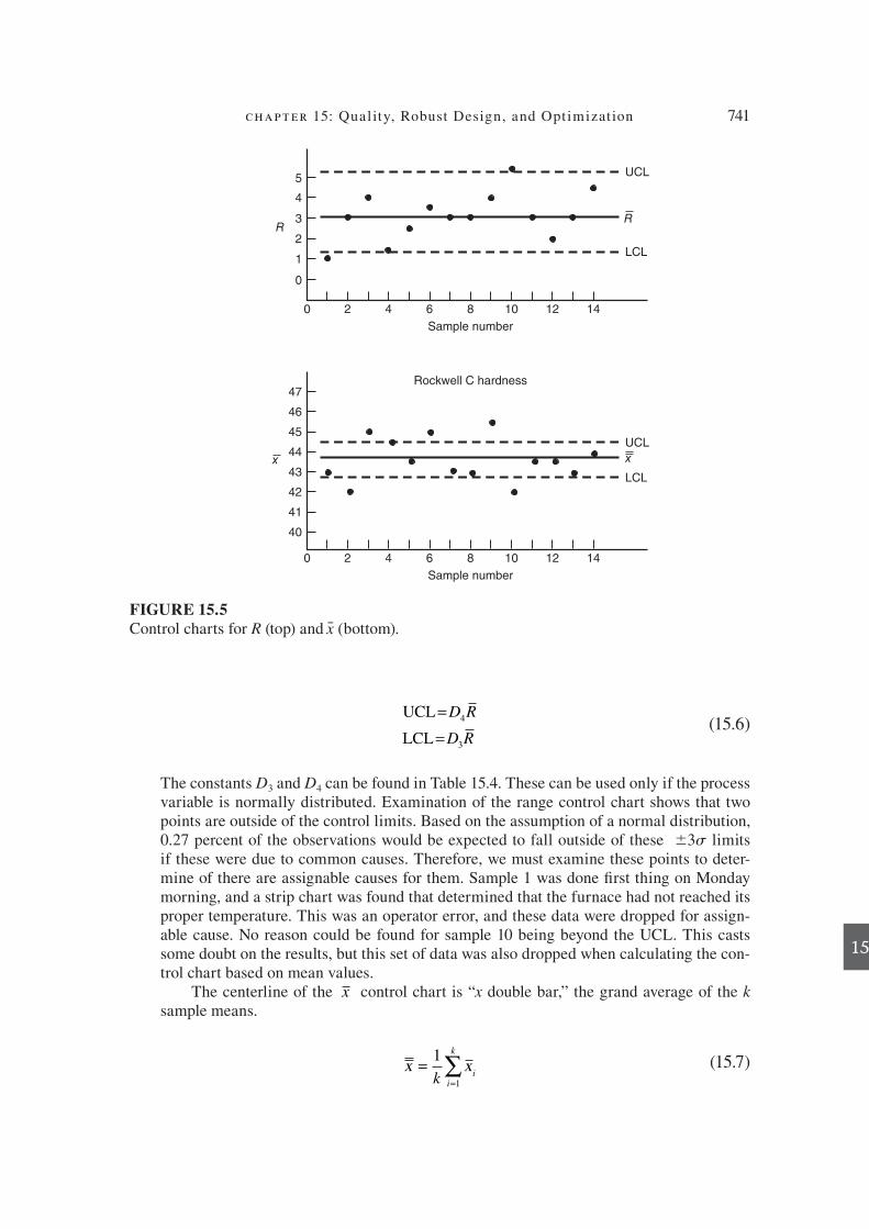
chapter 15: Qual ity, Robust Design, and Optimizat ion 741
15
UCL
LCL
=
=
D R
D R
4
3
(15.6)
The constants D 3 and D 4 can be found in Table 15.4. These can be used only if the process variable is normally distributed. Examination of the range control chart shows that two points are outside of the control limits. Based on the assumption of a normal distribution, 0.27 percent of the observations would be expected to fall outside of these 3s limits if these were due to common causes. Therefore, we must examine these points to deter-mine of there are assignable causes for them. Sample 1 was done a rst thing on Monday morning, and a strip chart was found that determined that the furnace had not reached its proper temperature. This was an operator error, and these data were dropped for assign-able cause. No reason could be found for sample 10 being beyond the UCL. This casts some doubt on the results, but this set of data was also dropped when calculating the con-trol chart based on mean values.
The centerline of the x control chart is “ x double bar,” the grand average of the k sample means.
x x==∑1
1k ii
k
(15.7)
0
40
41
42
43
44
45
46
47
2 4 6 8
Sample number
Rockwell C hardness
LCL
10 12 14
x
0
0
1
2
3
4
5
2 4 6 8
Sample number
UCL
R
LCL
10 12 14
R
UCL
x
FIGURE 15.5
Control charts for R (top) and x (bottom).
die37039_ch15.indd 741 2/25/08 7:02:02 PM

742 engineering design
15
Again, the UCL and LCL are set at 3s about the mean. If we knew the population mean and standard deviation, this would be given by UCL 5 µ σ+ ( )3 n , where the term in parentheses is the standard error of the mean. Since we do not know these parameters, the approximations for the control limits is
UCL
LCL
= +
= −
x A R
x A R
2
2
(15.8)
Note that the upper and lower control limits depend not only on the grand mean but also on the sample size, through A 2 , and the mean of the range.
The –x control chart shows many excursions of the mean outside of the control limits even after the control limits have been recalculated to eliminate the two out-of-control samples from the range chart. It is concluded that this particular batch of steel does not have sufa cient homogeneity of alloy content to respond consistently to heat treat-ment within such narrow specia cation limits.
15.5.2 Other Types of Control Charts
The –R and –x charts were the a rst types used for quality control. The range was chosen
to measure variability because of its ease of calculation in a period before electronic calculators made it quick and easy to calculate standard deviations. Also, for small sample sizes the range is a more efa cient statistic than the standard deviation.
Today it is much more convenient to use standard deviation in control charts. The average standard deviation –s of k samples is given by
s
ks
i
i
k
==∑1
1 (15.9)
Equation (15.9) represents the centerline of the s chart. The upper and lower control limits are found at the 3-sigma limits according to Equation (15.10).
UCL and LCL= =B s B s4 3
(15.10)
Sample size, n D 3 D 4 B 3 B 4 A 2 A 3 d 2 c 4
2 0 3.27 0 3.27 1.88 2.66 1.13 0.798
4 0 2.28 0 2.27 0.73 1.63 2.06 0.921
6 0 2.00 0.030 1.97 0.48 1.29 2.53 0.952
8 0.14 1.86 0.185 1.82 0.37 1.10 2.70 0.965
10 0.22 1.78 0.284 1.72 0.27 0.98 2.97 0.973
12 0.28 1.71 0.354 1.65 0.22 0.89 3.08 0.978
TABLE 15.4
Factors for Use in Determining Control Limit for Control Charts
die37039_ch15.indd 742 2/25/08 7:02:03 PM

chapter 15: Qual ity, Robust Design, and Optimizat ion 743
15
A control chart often is used to indicate a shift in the process mean during a pro-duction run. A succession of 6 to 10 points above or below the centerline of the chart is an indication of a shift in the mean. The sensitivity in detecting a mean shift can be increased by taking the deviation of each sample from the centerline and adding these in a cumulative way for each succeeding sample to form a CUSUM chart. 20
The preceding discussion of control charts was based on a variable measured on a continuous quantitative scale . Often in inspection it is quicker and cheaper to check the product on a go/no-go basis . The part is either “not defective” or “defective” based on a gage or predetermined specia cation. In this type of attribute testing, we deal with the fraction or proportion of defects in a sample. The p chart , based on the binomial distribution, deals with the fraction of defective parts in a sample over a succession of samples. The c chart , based on the Poisson distribution, monitors the number of de-fects per sample. Other important issues in statistical quality control are the design of sampling plans and the intricacies of sampling parts on the production line. 21
15.5.3 Determining Process Statistics from Control Charts
Because control charts are commonly determined for manufacturing processes, they are a useful source of process statistics for determining the process capability index, Sec. 15.4. The grand average x of the means of k samples, Eq. (15.7), is the best esti-mate for the process mean m .
The estimate of the process standard deviation is given by Eq. (15.11), depend-ing on whether the R chart or s chart has been used to measure the variability in the process.
ˆ ˆσ σ= =R
d
s
c2 4
or (15.11)
All of the equations for determining the process parameters are based on the assump-tion that they follow a normal distribution.
15.6 TAGUCHI METHOD
A systematized statistical approach to product and process improvement has devel-oped in Japan under the leadership of Dr. Genichi Taguchi. 22 This took a total qual-ity emphasis but developed quite unique approaches and terminology. It emphasizes
20. W . Navidi , Statistics for Engineers and Scientists, 2d ed., pp. 782–84 , McGraw-Hill, New York , 2008 . 21. D. H . Bestera eld , Quality Control, 5th ed., Prentice Hall, Upper Saddle River, NJ , 1998 ; A . Mitra , Fundamentals of Quality Control and Improvement, 2d ed., Prentice Hall, Upper Saddle River, NJ, 1998 .
22. G . Taguchi , Introduction to Quality Engineering, Asian Productivity Organization, Tokyo , 1986 , available from Kraus Int. Publ., White Plains, NY ; G . Taguchi , Taguchi on Robust Technology Develop-
ment, ASME Press, New York , 1993 .
die37039_ch15.indd 743 2/25/08 7:02:03 PM

744 engineering design
15
moving the quality issue upstream to the design stage and focusing on prevention of defects by process improvement. Taguchi has placed great emphasis on the impor-tance of minimizing variation as the primary means of improving quality. Special attention is given to the idea of designing products so that their performance is insen-sitive to changes in the environment in which the product functions, also called noise. The process of achieving this through the use of statistically designed experiments has been called robust design (see Sec. 15.7).
15.6.1 Loss Function
Taguchi dea nes the quality level of a product to be the total loss incurred by society due to the failure of the product to deliver the expected performance and due to harm-ful side effects of the product, including its operating cost. This may seem a backward dea nition of quality because the word quality usually denotes desirability, while the word loss conveys the impression of undesirability. In the Taguchi concept some loss is inevitable because of the realities of the physical world from the time a product is shipped to the customer and the time it is put in use. Thus, all products will incur some quality loss. The smaller the loss, the more desirable the product.
It is important to be able to quantify this loss so that alternative product designs and manufacturing processes can be compared. This is done with a quadratic loss function (Fig. 15.6 a ):
L y k y m( ) = −( )2
(15.12)
where L ( y ) is the quality loss when the quality characteristic is y , m is the target value for y, and k is a constant, the quality loss coefa cient.
Figure 15.6 a shows the loss function for the common situation where the speci-a cation on a part is set at a target value, m , with a bilateral tolerance band #. The conventional approach to quality considers any dimension that falls within the toler-ance range to be a good part, and any dimension outside of the USL-LSL region is a defective part. The analogy can be made to the goalposts in football, where any kick that went through the uprights is a score, no matter how close it came to the upright. In football, no extra points are awarded for a kick that goes right between the middle of the goal posts.
Taguchi argues that this conventional approach is not realistic for dea ning qual-ity. While it may be reasonable in football to award the same score so long as the ball falls in the interval 2∆, for a quality engineering approach where variability is the enemy of quality, any deviation from the design target is undesirable and degrading to quality. Moreover, dea ning the loss function as a quadratic instead of a linear expres-sion emphasizes the importance of being close to the target value.
It is evident from Fig. 15.6 a that y exceeds the tolerance ∆ when L(y) = A . A is the loss incurred when a product falls outside of the tolerance range and is re-jected, or when a part in service needs to be repaired or replaced. When this occurs,
y m= = + ∆USL . Substituting into Eq. (15.12),
die37039_ch15.indd 744 2/25/08 7:02:03 PM

chapter 15: Qual ity, Robust Design, and Optimizat ion 745
15
L m A k m m k
k A
+ ∆( ) = = + ∆( ) − = ∆
= ∆
22
2/
Substituting into Eq. (15.12) gives:
L y
Ay m( ) =
∆−( )2
2
(15.13)
This is the form of the quality loss equation that is most often used for the case where the highest quality (lowest loss) is achieved when the quality characteristic is as close as possible to the target value, and it is symmetrical about the target. Note that L ( y ) = 0 only when y = m . A CTQ dimension on a part is an example of a nominal-is-better design parameter.
Two other common situations are shown in Fig. 15.6, along with the appropri-ate equation for the loss function. Figure 15.6 b illustrates the case where the ideal value is zero and the smallest deviation from this target produces the highest quality. An example would be if y represented pollution from an automobile exhaust. Figure 15.6 c shows the opposite situation, where the largest deviation from zero would produce the lowest loss function. Design for the strength of a part would fall in this category.
A
A
L(y)
L(y)
L(y) = (y – m)2A2
ym
(a) Nominal-the-best
m – m +
y0
L(y) = y2A2
(b) Smaller-the-better
A
L(y)
y0
L(y)1
=y2
A 2
(c) Larger-the-better
(a)
(b)
(c)
FIGURE 15.6
Plots of the loss function curve for three common situations.
die37039_ch15.indd 745 2/25/08 7:02:04 PM

746 engineering design
15
E X A M P L E 1 5 . 6 A power supply for an electronic product must deliver a nominal output voltage of 115 volts. When the output voltage varies from the nominal by more than 20 volts, the customer will experience degraded performance or the product will be damaged and repairs will be nec-essary at an average cost of $100. What is the loss if the product is shipped with a power supply having an output of 110 volts? From this statement of the problem we may write:
m y A k= = ∆ = = = ∆ =115 110 20 100 1002volts volts $ / /A 220 0 25
110 0 25 110 1
2
2
( ) =
( ) = −( ) = −
$ . /
$ .
volts
L k y m 115 6 252( ) = $ .
This is the customer’s perceived quality loss when the power supply delivers 110 instead of 115 volts.
E X A M P L E 1 5 . 7
Suppose the manufacturer could recalibrate the power supply at the end of the production line to bring it closer to the target voltage. Whether this should be done, from an eco-nomic point of view, depends upon whether the cost of repair is less than the customer’s perceived quality loss. In this case, let A 5 cost of rework 5 $3 per unit. How great should the deviation from target be before the manufacturer should rework the power sup-ply? The loss to the customer is given in Example 15.6.
L y y m y m
L y
( ) = −( ) = − ∆
( ) =
0 25
3
2.
$
and
at the decision point
3 0 25 0 253
0 2512 3 46
2 2= − ∆ −( ) = ∆ ∆ = = =. ..
.m m volts
Providing that the output voltage is within 3.5 volts of the target (115 v) the manufacturer should not spend $3 per unit to recalibrate the unit. This value is the manufacturer’s eco-nomic tolerance limit. Beyond this point the customer’s loss increases beyond acceptable limits.
The average quality loss of a sample of products, obtained by summing the individual losses and dividing by their number, is given by: 23
L y k y m( ) = + −( )
σ 2 2
(15.14)
where −L(y) is the average quality loss s2 is the population variance on y due to common causes in the pro-
cess. It usually is approximated by the sample variance
–y is the mean of all yi in the sample, or m as dea ned in Sec. 15.5.3. ( –y 2 m)2 is the square of the deviation of –y from the target value m , due to assignable variation.
23. W. Y . Fowlkes and C. M . Creveling , Engineering Methods for Robust Product Design, Chap. 3, Addison-Wesley, Reading, MA , 1995 .
die37039_ch15.indd 746 2/25/08 7:02:04 PM

chapter 15: Qual ity, Robust Design, and Optimizat ion 747
15
Equation (15.14) is an important relationship because it breaks the quality loss into the component of the loss that is due to product or process variability and the amount that is due to the mean of the sample being displaced from the target value.
E X A M P L E 1 5 . 8
A manufacturing process has a standard deviation of 0.00226 inches and a mean of 1.503 inches (see Example 15.4). The specia cation for the CTQ dimension of the part is 1.500 0.009 inches. The part can no longer be assembled into a subsystem if y exceeds 1.5009 and it is reworked at a cost of $16.
(a) What is the average quality loss for parts made from this process?
First we need to a nd the quality loss coefa cient, k , for the process.
k A
L y k
= ∆ = ( ) =
( ) =
/ $ / . , $/
ˆ
2 2 216 0 009 197 531 in.
σσ µ2 2 2
197 531 0 00226 1 503 1+ −( )
= ( ) + −ˆ , . .m ..5002( )
= × + × − −197 531 5 108 10 9 106 6, . = $ .2 787
Note that the quality loss due to the shift of the mean is about twice that due to process variability.
(b) If the process mean is centered with the target mean for the part, what is the quality loss factor?
Now ( m2m) 5 (1.50021.500) 5 0 and the quality loss factor is due entirely due to variation of the process.
–L (y) 5 197,531(5.108 3 1026) 5 $1.175
As we will see in Sec. 15.7, the usual approach using the Taguchi method is to a rst search for choices of the design parameters that minimize the product’s suscep-tibility to variation, and then having found the best combination, adjust the process conditions to bring the product mean and the process mean into coincidence.
15.6.2 Noise Factors
The input parameters that affect the quality of the product or process may be clas-sia ed as design parameters and disturbance factors. The former are parameters that can be specia ed freely by the designer. It is the designer’s responsibility to select the optimum levels of the design parameters. Disturbance factors are the parameters that are either inherently uncontrollable or impractical to control.
Taguchi uses the term noise factors to refer to those parameters that are either too difa cult or too expensive to control when a product is in service or during manufac-ture of its components. The noise factors can be classia ed into four categories:
Variational noise is the unit-to-unit variation that nominally identical products will exhibit due to the differences in their components or their assembly.
Inner noise is the long-term change in product characteristics over time due to dete-rioration and wear.
●
●
die37039_ch15.indd 747 2/25/08 7:02:05 PM
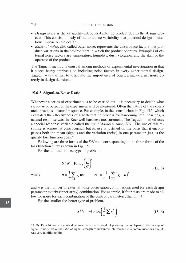
748 engineering design
15
Design noise is the variability introduced into the product due to the design pro-cess. This consists mostly of the tolerance variability that practical design limita-tions impose on the design.
External noise , also called outer noise, represents the disturbance factors that pro-duce variations in the environment in which the product operates. Examples of ex-ternal noise factors are temperature, humidity, dust, vibration, and the skill of the operator of the product.
The Taguchi method is unusual among methods of experimental investigation in that it places heavy emphasis on including noise factors in every experimental design. Taguchi was the a rst to articulate the importance of considering external noise di-rectly in design decisions.
15.6.3 Signal-to-Noise Ratio
Whenever a series of experiments is to be carried out, it is necessary to decide what response or output of the experiment will be measured. Often the nature of the experi-ment provides a natural response. For example, in the control chart in Fig. 15.5, which evaluated the effectiveness of a heat-treating process for hardening steel bearings, a natural response was the Rockwell hardness measurement. The Taguchi method uses a special response variable called the signal-to-noise ratio , S/N . The use of this re-sponse is somewhat controversial, but its use is justia ed on the basis that it encom-passes both the mean (signal) and the variation (noise) in one parameter, just as the quality loss function does. 24
Following are three forms of the S/N ratio corresponding to the three forms of the loss function curves shown in Fig. 15.6.
For the nominal-is-best type of problem,
S N
nyi
n
/ =
==
∑
102
1
log
l andl
µσ
µ σσ µ2 2
1
11
=−
−( )=∑n
yii
n (15.15)
where
and n is the number of external noise observation combinations used for each design parameter matrix (inner array) combination. For example, if four tests are made to al-low for noise for each combination of the control parameters, then n = 4.
For the smaller-the-better type of problem,
S Nn
yi
/ = −
∑10 2 log
l (15.16)
●
●
24 . Dr. Taguchi was an electrical engineer with the national telephone system of Japan, so the concept of signal-to-noise ratio, the ratio of signal strength to unwanted interference in a communications circuit, was very familiar to him.
die37039_ch15.indd 748 2/25/08 7:02:05 PM
chapter 15: Qual ity, Robust Design, and Optimizat ion 749
15
For the larger-the-better type of problem, the quality performance characteristic is continuous and nonnegative. We would like y to be as large as possible. To Y nd the S/N, we turn this into a smaller-the-better problem by using the reciprocal of the per-formance characteristic.
S Nn yi
/ = −
∑10 2log l l
(15.17)
15.7 ROBUST DESIGN
Robust design is the systematic approach to Y nding optimum values of design factors that lead to economical designs with low variability. The Taguchi method achieves this goal by Y rst performing parameter design, and then, if the outcomes still are not optimum, by performing tolerance design.
Parameter design 25 is the process of identifying the settings of the design param-eters or process variables that reduce the sensitivity of the design to sources of varia-tion. This is done in a two-step process. First, control factors are identiY ed. These are design parameters that primarily affect the S/N ratio but not the mean. Using statistically planned experiments, we Y nd the level of the control factors that mini-mize the variability of the response. Once the variance has been reduced, the mean response can be adjusted by using a suitable design parameter, known as the signal
factor .
15.7.1 Parameter Design
Parameter design makes heavy use of planned experiments. The approach involves statistically designed experiments that are based on fractional factorial designs. 26 With factorial designs only a small fraction of the total number of experiments must be performed when compared with the conventional approach of varying one parameter at a time in an exhaustive testing program. The meaning of a fractional factorial design is shown in Fig. 15.7. Suppose we identify three control parameters (factors) P 1 , P 2 , and P 3 that in uence the performance of the design. We want to de-termine their in uence on the objective function. The response is measured at two levels of the design parameters, one low (1) and one high (2). In the conventional ap-proach of varying one factor at a time, this would require 2 3 = 8 tests as illustrated in Fig. 15.7 a . However, if we use a fractional factorial Design of Experiment (DoE), essentially the same information is obtained with half as many tests, as illustrated
25 . The terminology is a bit tenuous. The process called parameter design is Y rmly established in the Taguchi method for robust design. This work is generally conducted in the parametric design stage of the embodiment phase of the design process. 26. W . Navidi , op. cit, pp. 735–38 .
die37039_ch15.indd 749 2/25/08 7:02:06 PM

750 engineering design
15
in Fig. 15.7 b . All common fractional factorial designs are orthogonal arrays. These arrays have the balancing property that every setting of a design parameter occurs with every setting of all other design parameters the same number of times. They keep this balancing property while minimizing the number of test runs. Taguchi presented the orthogonal arrays in an easy-to-use form that uses only parts of the fractional factorial test plan. The trade-off is that the number of tests is minimized, but detailed information about interactions is lost.
Figure 15.8 shows two commonly used orthogonal arrays. The columns represent the control factors, A, B, C, and D, and the rows represent the setting of the param-eters for each experimental run. The L4 array deals with three control factors at two levels, while the L9 array considers four factors each at three levels. Note that the L9 array reduces the full experiment of 3 4 5 81 runs to only 9 experimental runs. This reduction is accomplished by confounding the interaction effects (AB, etc.) with the main effects (A, B, etc.). Note also the balance between the levels of the control fac-tors. Each level for each control factor appears in the same number of runs. For ex-ample, level 1 of B appears in runs 1 , 4, and 7; level 2 occurs in runs 2, 5, and 8, while level 3 occurs in runs 3, 6, and 9. This balance between control factor levels allows averages to be computed that isolate the effect of each factor.
The choice of which orthogonal array to use depends on the number of control factors and noise factors. 27 The decision of whether to use an array with factors at two or three levels depends on whether you are seeking more resolution in the results, es-pecially if you feel the responses will be nonlinear. Of course, the number of control and noise factors determines the resources needed for the investigation.
P2 P2
P1
(a) (b)
Test conducted
Test omitted
P1
P3 P3
FIGURE 15.7
Designed experiment plan. Three factors P tested at two levels. (a) All test combinations considered. (b) Fractional factorial design
27. G . Taguchi , System of Experimental Design: Engineering Methods to Optimize Quality and Mini-
mize Cost, 2 vols., Quality Resources, White Plains, NY , 1987 ; M. S . Phadke , Quality Engineering Using
Robust Design, Prentice Hall, Upper Saddle River, NJ , 1989 ; W. Y . Fowlkes and C. M . Creveling , op. cit., Appendix C.
die37039_ch15.indd 750 2/25/08 7:02:06 PM

chapter 15: Qual ity, Robust Design, and Optimizat ion 751
15
Suppose y 1 , y 2 . . . y 9 are the results of the response measured in each of the nine runs. Let
–yB1
be the response averaged over those runs where B is at level 1 in the L9 array; –yB2 averaged over those runs where B is at level 2, and so on. Then we may write:
y y y y
y y y y
y y y y
B
B
B
1 1 4 7
2 2 5 8
3 3 6 9
3
3
3
= + +( )= + +( )= + +( )
/
/
/
(15.18)
Similar equations would be developed for –y Ai, –yCi , and –yDi .
The Taguchi design of experiments usually consists if two parts. The Y rst part is a design parameter matrix from which the effects of the control parameters are determined through the use of a suitable orthogonal array. The second part is the noise matrix, a smaller orthogonal array consisting of noise parameters. Often the Y rst matrix is called the inner array and the noise matrix is termed the outer array. It is common to use an L9 array with nine runs for the inner array and an L4 array with four runs for the outer array. Thus, for run 1 in the L9 array [all factors at the low (1) level] there are four trials, one for each combination of factors in the noise matrix, the L4 array. For run 2 there are another four trials, etc., so that a total of 9 3 4 5 36 test conditions will be evaluated. The responses are evaluated for each of the four trials in the Y rst run and statistics like the mean and standard deviation are deter-mined. This evaluation is performed for each of the nine runs for the design parameter matrix.
The creation of a robust design using the Taguchi Method proceeds in six steps:
DeY ne the problem, including the selection of the parameter to be optimized and the objective function. Select the design parameters—often called the control factors, and the noise fac-tors. The control factors are parameters under the control of the designer that may be calculated or determined experimentally. The noise factors are those param-eters that contribute to the variation caused by the environment.
1.
2.
1
2
3
4
1
2
3
4
5
6
7
8
9
1
1
1
2
2
2
3
3
3
1
2
3
1
2
3
1
2
3
1
2
3
2
3
1
3
1
2
1
2
3
3
1
2
2
3
1
1
1
2
2
1
L4 ARRAY
L9 ARRAY
Run No.
Run
No.A B C D
A B C
2
1
2
1
2
2
1
FIGURE 15.8
Orthogonal arrays; left, the L4 array and right, the L9 array.
die37039_ch15.indd 751 2/25/08 7:02:07 PM
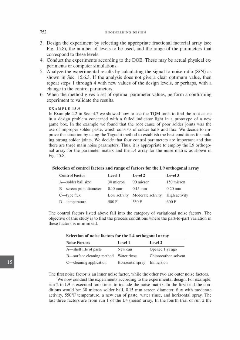
752 engineering design
15
Design the experiment by selecting the appropriate fractional factorial array (see Fig. 15.8), the number of levels to be used, and the range of the parameters that correspond to these levels. Conduct the experiments according to the DOE. These may be actual physical ex-periments or computer simulations. Analyze the experimental results by calculating the signal-to-noise ratio (S/N) as shown in Sec. 15.6.3. If the analysis does not give a clear optimum value, then repeat steps 1 through 4 with new values of the design levels, or perhaps, with a change in the control parameters. When the method gives a set of optimal parameter values, perform a conY rming experiment to validate the results.
E X A M P L E 1 5 . 9
In Example 4.2 in Sec. 4.7 we showed how to use the TQM tools to Y nd the root cause in a design problem concerned with a failed indicator light in a prototype of a new game box. In the example we found that the root cause of poor solder joints was the use of improper solder paste, which consists of solder balls and ux. We decide to im-prove the situation by using the Taguchi method to establish the best conditions for mak-ing strong solder joints. We decide that four control parameters are important and that there are three main noise parameters. Thus, it is appropriate to employ the L9 orthogo-nal array for the parameter matrix and the L4 array for the noise matrix as shown in Fig. 15.8.
3.
4.
5.
6.
Control Factor Level 1 Level 2 Level 3
A—solder ball size 30 micron 90 micron 150 micron
B—screen print diameter 0.10 mm 0.15 mm 0.20 mm
C—type ux Low activity Moderate activity High activity
D—temperature 500 F 550 F 600 F
Selection of control factors and range of factors for the L9 orthogonal array
The control factors listed above fall into the category of variational noise factors. The objective of this study is to Y nd the process conditions where the part-to-part variation in these factors is minimized.
Noise Factors Level 1 Level 2
A—shelf life of paste New can Opened 1 yr ago
B—surface cleaning method Water rinse Chlorocarbon solvent
C—cleaning application Horizontal spray Immersion
Selection of noise factors for the L4 orthogonal array
The Y rst noise factor is an inner noise factor, while the other two are outer noise factors. We now conduct the experiments according to the experimental design. For example,
run 2 in L9 is executed four times to include the noise matrix. In the Y rst trial the con-ditions would be: 30 micron solder ball, 0.15 mm screen diameter, ux with moderate activity, 550°F temperature, a new can of paste, water rinse, and horizontal spray. The last three factors are from run 1 of the L4 (noise) array. In the fourth trial of run 2 the
die37039_ch15.indd 752 2/25/08 7:02:07 PM

chapter 15: Qual ity, Robust Design, and Optimizat ion 753
15
conditions for L9 would be identical, but the noise factors would change to using a can of paste opened one year ago, a chlorocarbon cleaning agent, and horizontal spray for clean-ing. For each of the four trials of run 2, we measure a response that represents the objec-tive function that we are attempting to optimize. In this case, the response is the shear strength of the solder joint measured at room temperature. For the four trials, we average the strength measurements and determine the standard deviation. For run 2, the results are:
y2
4 175 4 301 3 019 3 3134 4 3 657= + + +( ) =. . . . / . ksi
andd σ =−( )
−=∑ y y
n
i2 2
2
10 584.
In robust design the appropriate response parameter is the signal-to-noise ratio. Because we are trying to Y nd the conditions to maximize the shear strength of the solder joints, the larger-is-best form of the S/N is selected.
S Nn y
i
/ = −
∑10
12
log1
For each of the runs in the L9 array we calculate a signal-to-noise ratio. For run 2,
S Nrun
/. . .
( ) = −( )
+( )
+2 2 2
101
4
1
4 175
1
4 301
1
3 01log
99
1
3 13410 09
2 2( )+
( )
=
..
The following table shows the results of similar calculations for all of the runs in the pa-rameter matrix. 28
Run No. Control Matrix S/N
A B C D
1 1 1 1 1 9.89
2 1 2 2 2 10.09
3 1 3 3 3 11.34
4 2 1 2 3 9.04
5 2 2 3 1 9.08
6 2 3 1 2 9.01
7 3 1 3 2 8.07
8 3 2 1 3 9.42
9 3 3 2 1 8.89
28 . Note that these numbers are to illustrate the design method. They should not be considered to be valid design data.
die37039_ch15.indd 753 2/25/08 7:02:08 PM
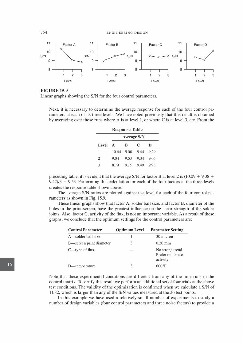
754 engineering design
15
Next, it is necessary to determine the average response for each of the four control pa-rameters at each of its three levels. We have noted previously that this result is obtained by averaging over those runs where A is at level 1, or where C is at level 3, etc. From the
S/N
11
10
9
8
1 2 3
Level
Factor A
S/N
11
10
9
8
1 2 3
Level
Factor B
S/N
11
10
9
8
1 2 3
Level
Factor C
S/N
11
10
9
8
1 2 3
Level
Factor D
FIGURE 15.9
Linear graphs showing the S/N for the four control parameters.
Average S/N
Level A B C D
1 10.44 9.00 9.44 9.29
2 9.04 9.53 9.34 9.05
3 8.79 9.75 9.49 9.93
Response Table
preceding table, it is evident that the average S/N for factor B at level 2 is (10.09 1 9.08 1 9.42)/3 5 9.53. Performing this calculation for each of the four factors at the three levels
creates the response table shown above. The average S/N ratios are plotted against test level for each of the four control pa-
rameters as shown in Fig. 15.9. These linear graphs show that factor A, solder ball size, and factor B, diameter of the
holes in the print screen, have the greatest in uence on the shear strength of the solder joints. Also, factor C, activity of the ux, is not an important variable. As a result of these graphs, we conclude that the optimum settings for the control parameters are:
Control Parameter Optimum Level Parameter Setting
A—solder ball size 1 30 micron
B—screen print diameter 3 0.20 mm
C—type of ux — No strong trend Prefer moderate activity
D—temperature 3 600°F
Note that these experimental conditions are different from any of the nine runs in the control matrix. To verify this result we perform an additional set of four trials at the above test conditions. The validity of the optimization is conY rmed when we calculate a S/N of 11.82, which is larger than any of the S/N values measured at the 36 test points.
In this example we have used a relatively small number of experiments to study a number of design variables (four control parameters and three noise factors) to provide a
die37039_ch15.indd 754 2/25/08 7:02:08 PM

chapter 15: Qual ity, Robust Design, and Optimizat ion 755
15
new set of control parameters that are closer to an optimum than an informed guess, and which are robust to the noise factors.
15.7.2 Tolerance Design
Often, as in Example 15.9, the parameter design results in a design optimized for robustness and with a low variability. However, there are situations when the variabil-ity is too large and it becomes necessary to reduce tolerances to decrease variability. Typically, analysis of variance (ANOVA) is used to determine the relative contribution of each control parameter so as to identify those factors that should be considered for tolerance tightening, substituting an improved material, or some other means of im-proving quality. Since these methods often incur additional cost, the Taguchi method of tolerance design provides careful methods for balancing increased quality (lower quality loss) with cost. This tolerance design methodology is beyond the scope of this text, but an excellent, readable source is available. 29
Taguchi’s methods of quality engineering have generated great interest in the United States as many major manufacturing companies have embraced the approach. While the idea of loss function and robust design is new and important, many of the statistical techniques have been in existence for over 50 years. Statisticians point out 30 that less complicated and more efY cient methods exist to do what the Taguchi meth-ods accomplish. However, it is important to understand that before Taguchi system-atized and extended these ideas into an engineering context, they were largely unused by much of industry. The growing acceptance of the Taguchi method comes from its applicability to a wide variety of industrial problems with a methodology that does not require a high level of mathematical skills to achieve useful results.
15.8 OPTIMIZATION METHODS
The example described in the previous section is a search for the best combination of design parameters using a statistically designed set of experiments when the desired outcome is clear. There is more than one solution to a design problem, and the Y rst solution is not necessarily the best. Thus, the need for optimization is inherent in the design process. A mathematical theory of optimization has become highly developed and is being applied to design where design functions can be expressed mathemati-cally. The applicability of the mathematical methods usually depends on the existence of a continuously differentiable objective function. Where differentiable equations cannot be developed, numerical methods, aided by computer-based computation, are used to carry out optimization. These optimization methods require considerable depth of knowledge and mathematical skill to select the appropriate optimization technique and work it through to a solution.
29. C. M . Creveling , Tolerance Design: A Handbook for Developing Optimal Speci! cations, Addison-Wesley Longman, Reading, MA , 1997 . 30. R. N . Kackar , Jnl of Quality Tech., Vol. 17, no. 4, pp. 176–209 , 1985 .
die37039_ch15.indd 755 2/25/08 7:02:09 PM

756 engineering design
15
By the term optimal design we mean the best of all feasible designs. Optimization is the process of maximizing a desired quantity or minimizing an undesired one. Op-timization theory is the body of mathematics that deals with the properties of maxima and minima and how to Y nd maxima and minima numerically. In the typical design optimization situation, the designer has deY ned a general conY guration for which the numerical values of the independent variables have not been Y xed. An objective func-
tion 31 that deY nes the overall value of the design in terms of the n design variables, expressed as a vector x , is established.
f f x x xn
x( ) = ( )1 2, , . . . (15.19)
Typical objective functions can be expressed in terms of cost, weight, reliability, and material performance index or a combination of these. By convention, objective func-tions are usually written to minimize their value. However, maximizing a function f ( x ) is the same as minimizing – f ( x ).
Generally when we are selecting values for a design we do not have the freedom to select arbitrary points within the design space. Most likely the objective function is subject to certain constraints that arise from physical laws and limitations or from compatibility conditions on the individual variables. Equality constraints specify re-lations that must exist between the variables.
h h x x x j pj j n
x( ) = ( ) = =1 2
0 1, , . . . ; to (15.20)
For example, if we were optimizing the volume of a rectangular storage tank, where x 1 5 l 1 , x 2 5 l 2 , and x 3 5 l 3 , then the equality constraint would be volume V = l1, l2, l3. The number of equality constraints must be no more than the number of design vari-ables, p ≤ n .
Inequality constraints , also called regional constraints, are imposed by speciY c details of the problem.
g g x x x i mi i n
x( ) = ( ) ≤ =1 2
0 1, , . . . ; to (15.21)
There is no restriction on the number of inequality constraints. 32 A type of inequality constraint that arises naturally in design situations is based on speciY cations. Speci! -
cations deY ne points of interaction with other parts of the system. Often a speciY ca-tion results from an arbitrary decision to carry out a suboptimization of the system by establishing a Y xed value for one of the design variables.
A common problem in design optimization is that there often is more than one design characteristic that is of value to the user. One way to handle this case in for-mulating the optimization problem is to choose one predominant characteristic as the objective function and to reduce the other characteristics to the status of constraints. Frequently they show up as rather “hard” or severely deY ned speciY cations. In reality,
31 . Also called the criterion function, the payoff function, or cost function.
32. It is conventional to write Eq. (15.21) as #0. If the constraint is of the type $ 0, convert to this form by multiplying through by 21.
die37039_ch15.indd 756 2/25/08 7:02:10 PM
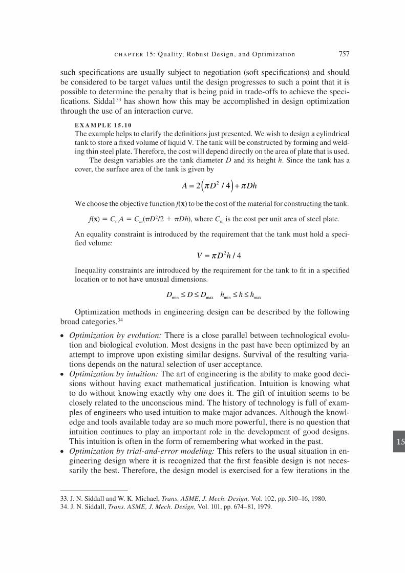
chapter 15: Qual ity, Robust Design, and Optimizat ion 757
15
such speciY cations are usually subject to negotiation (soft speciY cations) and should be considered to be target values until the design progresses to such a point that it is possible to determine the penalty that is being paid in trade-offs to achieve the speci-Y cations. Siddal 33 has shown how this may be accomplished in design optimization through the use of an interaction curve.
E X A M P L E 1 5 . 1 0
The example helps to clarify the deY nitions just presented. We wish to design a cylindrical tank to store a Y xed volume of liquid V. The tank will be constructed by forming and weld-ing thin steel plate. Therefore, the cost will depend directly on the area of plate that is used.
The design variables are the tank diameter D and its height h . Since the tank has a cover, the surface area of the tank is given by
A D Dh= ( ) +2 42π π/
We choose the objective function f ( x ) to be the cost of the material for constructing the tank.
f(x) 5 CmA 5 Cm(pD2/2 1 pDh), where C m is the cost per unit area of steel plate.
An equality constraint is introduced by the requirement that the tank must hold a speci-Y ed volume:
V D h= π 2 4/
Inequality constraints are introduced by the requirement for the tank to Y t in a speciY ed location or to not have unusual dimensions.
D D D h h hmin max ≤ ≤ ≤ ≤min max
Optimization methods in engineering design can be described by the following broad categories. 34
Optimization by evolution: There is a close parallel between technological evolu-tion and biological evolution. Most designs in the past have been optimized by an attempt to improve upon existing similar designs. Survival of the resulting varia-tions depends on the natural selection of user acceptance.
Optimization by intuition: The art of engineering is the ability to make good deci-sions without having exact mathematical justiY cation. Intuition is knowing what to do without knowing exactly why one does it. The gift of intuition seems to be closely related to the unconscious mind. The history of technology is full of exam-ples of engineers who used intuition to make major advances. Although the knowl-edge and tools available today are so much more powerful, there is no question that intuition continues to play an important role in the development of good designs. This intuition is often in the form of remembering what worked in the past.
Optimization by trial-and-error modeling: This refers to the usual situation in en-gineering design where it is recognized that the Y rst feasible design is not neces-sarily the best. Therefore, the design model is exercised for a few iterations in the
●
●
●
33. J. N . Siddall and W. K . Michael , Trans. ASME, J. Mech. Design, Vol. 102, pp. 510–16 , 1980 . 34. J. N . Siddall , Trans. ASME, J. Mech. Design, Vol. 101, pp. 674–81 , 1979 .
die37039_ch15.indd 757 2/25/08 7:02:10 PM

758 engineering design
15
hope of Y nding an improved design. This works best when the designer has suf-Y cient experience to make an informed choice of initial design values. The para-metric design of a spring in Sec. 8.5.2 is an example of this approach. However, this mode of operation is not true optimization. Some refer to this approach as sat-
is! cing , as opposed to optimizing, to mean a technically acceptable job done rap-idly and presumably economically. Such a design should not be called an optimal design.
Optimization by numerical algorithm: This approach to optimization, in which mathematically based strategies are used to search for an optimum, has been en-abled by the ready availability of fast, powerful digital computation. It is currently an area of active engineering research.
There are no universal optimization methods for engineering design. If the problem can be formulated by analytical mathematical expressions, then using the approach of calculus is the most direct path. However, most design problems are too complex to use this method, and a variety of optimization methods have been developed. Table 15.5 lists most of these methods. The task of the designer is to understand whether the problem is linear or nonlinear, unconstrained or constrained, and to select the method most applicable to the problem. Brief descriptions of various approaches to design op-timization are given in the rest of this section. For more depth of understanding about optimization theory, consult the various references given in Table 15.5.
Linear programming is the most widely applied optimization technique when constraints are known, especially in business and manufacturing production situ-ations. However, most design problems in mechanical design are nonlinear; see Example 15.10.
15.8.1 Optimization by Differential Calculus
We are all familiar with the use of the calculus to determine the maximum or mini-mum values of a mathematical function. Figure 15.10 illustrates various types of ex-trema that can occur. A characteristic property of an extremum is that f ( x ) is momen-tarily stationary at the point. For example, as point E is approached, f ( x ) increases, but right at E it stops increasing and the slope soon decreases. The familiar condition for a stationary point is
df
dx
x( )= 0 (15.22)
If the curvature is negative, then the stationary point is a maximum. The point is a minimum if the curvature is positive.
d f
dx
2
20
x( )≤ indicates a local maximum (15.23)
d f
dx
2
20
x( )≥ indicates a local minimum (15.24)
●
die37039_ch15.indd 758 2/25/08 7:02:11 PM

chapter 15: Qual ity, Robust Design, and Optimizat ion 759
15x
A
B
C
D
E
F
f(x)
FIGURE 15.10
Different types of extrema in the objective function curve.
Type of Algorithm Example Reference (see footnotes)
Linear programming Simplex method 1
Nonlinear programming Davison-Fletcher-Powell 2
Geometric programming 3
Dynamic programming 4
Variational methods Ritz 5
Differential calculus Newton-Raphson 6
Simultaneous mode design Structual optimization 7
Analytical-graphical methods Johnson’s MOD 8
Monotonicity analysis 9
Genetic algorithms 10
Simulated annealing 11
1. W. W . Garvin , Introduction to Linear Programming, McGraw-Hill, New York , 1960 .
2. M . Avriel , Nonlinear Programming: Analysis and Methods, Prentice Hall, Englewood Cliffs, NJ ,
1976 .
3. C. S . Beightler and D. T . Philips : Applied Geometric Programming, John Wiley & Sons, New
York , 1976 .
4. S. E . Dreyfus and A. M . Law , The Art and Theory of Dynamic Programming, Academic Press.
New York , 1977 .
5. M. H . Denn , Optimization by Variational Methods, McGraw-Hill, New York , 1969 .
6. F. B . Hildebrand , Introduction to Numerical Analysis, McGraw-Hill , 1956 .
7. L. A . Schmit (ed.), Structural Optimization Symposium, ASME, New York , 1974 .
8. R. C . Johnson , Optimum Design of Mechanical Elements, 2d ed., John Wiley & Sons, New York ,
1980 .
9. P. Y . Papalambros and D. J . Wilde , Principles of Optimal Design, 2d ed., Cambridge University
Press, New York , 2000 .
10. D. E . Goldberg , Genetic Algorithm, Addison-Wesley, Reading MA , 1989 .
11. S . Kirkpatrick , C. D . Gelatt , and M. P . Vecchi , “ Optimization by Simulated Annealing ,” Science,
Vol. 220, pp. 671–79 , 1983 .
TABLE 15.5
Listing of Numerical Methods Used in Optimization Problems
Both point B and point E are mathematical maxima. Point B , which is the smaller of the two maxima, is called a local maximum. Point E is the global maximum. Point D is a point of in ection. The slope is zero and the curve is horizontal, but the second derivative is zero. When d 2f(x)/dx2 5 0, higher-order derivatives must be used to Y nd a derivative that becomes nonzero. If the derivative is odd, the point is an in ection point, but if the derivative is even it is a local optimum. Point F is not a minimum
die37039_ch15.indd 759 2/25/08 7:02:11 PM

760 engineering design
15
point because the objective function is not continuous at it; the point F is only a cusp in the objective function. Using the derivative of the function to infer maxima or min-ima only works with a continuous function.
We can apply this simple optimization technique to the tank problem described in Example 15.10. The objective function, expressed in terms of the equality constraint V 5 pD2h/4, is
f x CD
C DhC D
C D VDm m
m
m( ) = + = +
−π ππ
ππ
2 2
2
2 2
4 (15.25)
df x
dDC D
C V
Dm
m( )
= = −04
2π (15.26)
DV
V=
=4
1 084
1 3
1 3
π
/
/. (15.27)
The value of diameter established by Eq. (15.27) results in minimum cost because the second derivative of Eq. (15.26) is positive. Note that while some problems yield to analytical expressions in which the objective function is a single variable, most engi-neering problems involve objective functions with more than one design variable.
Lagrange Multiplier Method
The Lagrange multipliers provide a powerful method for Y nding optima in multi-variable problems involving equality constraints. We have the objective function f(x) 5 f(x, y, z) subject to the equality constraints h1 5 h1(x, y, z) and h2 5 h2(x, y, z) . We establish a new function, the Lagrange expression (LE)
LE f x x y z h x y z h x y z= ( ) ( ) + ( ) + ( )2 1 1 2 2
, , , , , ,λ λ (15.28)
where l1 and l2 are the Lagrange multipliers. The following conditions must be satis-Y ed at the optimum point.
∂∂
=∂∂
=∂∂
=∂∂
=∂∂
=LE
x
LE
y
LE
z
LE LE0 0 0 0 0
1 2λ λ
(15.29)
E X A M P L E 1 5 . 1 1
This example illustrates the determination of the Lagrange multipliers for use in optimi-zation. 35 A total of 300 linear feet of tubes must be installed in a heat exchanger in order to provide the necessary heat-transfer surface area. The total dollar cost of the installation includes: (1) the cost of the tubes, $700; (2) the cost of the shell 25 D 25 L ; (3) the cost of the oor space occupied by the heat exchanger = 20 DL . The spacing of the tubes is such that
20 tubes must Y t in a cross-sectional area of 1 ft 2 inside the heat exchanger tube shell.
35. W. F . Stoecker , Design of Thermal Systems, 2d ed., McGraw-Hill, New York , 1980 .
die37039_ch15.indd 760 2/25/08 7:02:12 PM

chapter 15: Qual ity, Robust Design, and Optimizat ion 761
15
The purchase cost C is taken as the objective function. The optimization should de-termine the diameter D and the length of the heat exchanger L to minimize the purchase cost.
The objective function is the sum of three costs.
C D L DL= + +700 25 202 5. (15.30)
The optimization of C is subject to the equality constraint based on total length and cross-sectional area of the tube shell.
Total ft 3 of tubes 3 20 tubes/ft 2 = total length (ft).
π
π λπ
DL
D L LD
2
2
2
420 300
5 300300
5
× =
= = −
The Lagrange equation is: LE D L DL LD
= + + + −
700 25 20300
5
2 5
2
. λπ
∂∂
= ( ) + + =LE
DD L L
D2 5 25 20 2
6001 5
3. . λ
π (15.31)
∂∂
= + + =LE
LD D2 5 20 02 5. . λ (15.32)
∂∂
= − =LE
LDλ π
300
50
2 (15.33)
From Eq. From Eq. 15.3215 3360
2. , ;( ) = ( )L
Dπ25
Substituting into Eq.
2.5λ = − −
(D D20
15 31. ))
+
+ −
:
. .62 560
2060
2 251 5
2 2
2DD D
Dπ π
..5
320
600−( )
=DDπ
12 5 20 1 6 1 371 5 0 666. . .. .D D= = ( ) = ft
Substituting into the functional constraint, between D and L gives L = 10.2 ft. Sub-stituting the optimum values for D and L into the equation for the objective function, Eq. (15.30) gives the optimum cost as $1538.
This is an example of a closed form optimization for a single objective function with two design variables, D and L , and a single equality constraint.
die37039_ch15.indd 761 2/25/08 7:02:12 PM

762 engineering design
15
By their nature, design problems tend to have many variables, many constraints limiting the acceptable values of some variables, and many objective functions to de-scribe the desired outcomes of a design. A feasible design is any set of variables that simultaneously satisY es all the design constraints and fulY lls the minimum require-ments for functionality. An engineering design problem is usually underconstrained, meaning that there are not enough relevant constraints to set the value of each vari-able. Instead, there are many feasible values for each constraint. That means there are many feasible design solutions. As pointed out in the discussion of morphological methods (see Sec. 6.6), the number of feasible solutions grows exponentially as the number of variables with multiple possible values increases.
15.8.2 Search Methods
When it becomes clear that there are many feasible solutions to a design problem, it is necessary to use some method of searching through the space to Y nd the best one. Finding the globally optimal solution (the absolute best solution) to a design problem can be difY cult. There is always the option of using brute calculation power to iden-tify all design solutions and evaluate them. Unfortunately, design options reach into the thousands, and design performance evaluation can require multiple, complicated objective functions. Together, these logistical factors make an exhaustive search of the problem space impossible. There are also design problems that do not have one single best solution. Instead they may have a number of sets of design variable values that produce the same overall performance by combining different levels of the per-formance of one embedded objective function. In this case, we seek a set of best solu-tions. This set is called a Pareto set.
We can identify several classes of search problems. A deterministic search is one in which there is little variability of results and all problem parameters are known. In a stochastic search, there is a degree of randomness in the optimization process. We can have a search involving only a single variable or the more complicated and more realistic situation involving a search over multiple variables. We can have a si-
multaneous search , in which the conditions for every experiment are speciY ed and all the observations are completed before any judgment regarding the location of the optima is made, or a sequential search , in which future experiments are based on past outcomes. Many search problems involve constrained optimization , in which certain combinations of variables are forbidden. Linear programming and dynamic program-ming are techniques that deal well with situations of this nature.
Golden Section Search
The golden section search is an efY cient search method for a single variable with the advantage that it does not require an advance decision on the number of trials. The search method is based on the fact that the ratio of two successive Fibonacci numbers Fn21/Fn 5 0.618 for all values of n . 8. A Fibonacci series, named after a 13 th century mathematician, is given by Fn 5 Fn22 1 Fn21 where F0 5 1 and F1 5 1.
n
Fn
0 1 2 3 4 5 6 7 8 9
1 1 2 3 5 8 13 21 34 55. . .
die37039_ch15.indd 762 2/25/08 7:02:12 PM

chapter 15: Qual ity, Robust Design, and Optimizat ion 763
15
This same ratio was discovered by Euclid, who called it the golden mean . He deY ned it as a length divided into two unequal segments such that the ratio of the length of the whole to the larger segment is equal to the ratio of the length of the larger segment to the smaller segment. The ancient Greeks felt 0.618 was the most pleasing ratio of width to length of a rectangle, and they used it in the design of many of their buildings.
In using the golden section search, the Y rst two trials are located at 0.618 L from either end of the range of x that needs to be explored, Fig. 15.11. The goal is to Y nd the minimum value of the function or response. In the Y rst trial, x 1 5 0.618 L 5 6.18 and x 2 5 (1 2 0.618) L = 3.82. If y 2 . y 1 , the region to the left of x 2 is eliminated since we are searching for a minimum value of x and the assumption is that the function is unimodal.
For the second trial, the search interval L 2 is from x 5 3.82 to 10 5 6.18. The values of the two points are x 3 5 0.618(6.18) 1 3.82 5 7.64 (from 0 to the right) and x 4 5 10 2 6.18(0.618) 5 10 2 3.82 5 6.18 from x 5 0. Note that x 4 5 x 1 , so only one new data point is required. Once again, if y 4 . y 3 , we can eliminate the region to the left of y 4 . The new search interval is 3.82. The process is continued, placing a search point at 0.618 times the search interval, from both ends of the interval, until we reach as close to the minimum as is desired. Note that the golden section search cannot deal with functions that have multiple extrema between their limits. If this is suspected to occur, then start the search at one end of the domain and proceed in equal intervals across the limits.
Multivariable Search Methods
When the objective function depends on two or more variables, the geometric representation is a response surface (Fig. 15.12 a ). It usually is convenient to work with contour lines produced by the intersection of planes of constant y with the response surface and projected on the x 1 x 2 plane (Fig. 15.12 b ).
Lattice Search
In the lattice search, which is an analog to the single-variable search, a two-dimensional grid lattice is superimposed over the projections of the contours (Fig. 15.13). In the absence of special knowledge about the location of the maximum, the starting point is selected near the center of the region, at point 1. The objective
Trial 1 Trial 2
x2 =
3.8
2y =
f(x
)
x1 =
6.1
8
6.18
0 2 4 6 8 10x
L1
x3 =
7.6
4
x4 =
6.1
8
0 2 4 6 8 10x
L2
FIGURE 15.11
Example of use of the golden section search.
die37039_ch15.indd 763 2/25/08 7:02:13 PM

764 engineering design
15
3 4 5
2 1 6
9 8 7
x1
x2
FIGURE 15.13
Procedure for a lattice search.
y = 100
x2
y
x1
y = 90
0
x2
y = 100
y = 90
x1
(a) (b)
FIGURE 15.12
(a) Contour lines on surface created by x 1 x 2 ; (b) contour lines projected onto x 1 x 2 plane.
function is evaluated for points 1 through 9 surrounding point 1. If point 5 turns out to be the largest value, it becomes the central point for the next search. The procedure continues until the location reached is one at which the central point is greater than any of the other eight points. Frequently, a coarse grid is used initially and a Y ner grid is used after the maximum is approached.
Univariate Search
The univariate search is a one-variable-at-a-time method. All of the variables are kept constant except one, and it is varied to obtain an optimum in the objective function. That optimal value is then substituted into the function, and the function is
die37039_ch15.indd 764 2/25/08 7:02:13 PM

chapter 15: Qual ity, Robust Design, and Optimizat ion 765
15
optimized with respect to another variable. The objective function is optimized with respect to each variable in sequence, and an optimal value of a variable is substituted into the function for the optimization of the succeeding variables. This requires inde-pendence between the variables.
Figure 15.14 a shows the univariate search procedure. Starting at point 0 we move along x 2 = constant to a maximum by using a single-variable search technique. Then we move along x 1 = constant to a maximum at point 2 and along x 2 = constant to a maximum at 3. We repeat the procedure until two successive moves are less than some speciY ed value. If the response surface contains a ridge, as in Fig. 15.14 b , then the univariate search can fail to Y nd an optimum. If the initial value is at point 1, it will reach a maximum at x 1 = constant at the ridge, and that will also be a maximum for x 2 = constant. A false maximum is obtained.
An alternating single-variable search, as shown in Fig. 15.14, is sometimes used with the aid of a spreadsheet on a computer 36 when there are several design variables. The search procedure is to cycle through the design variables one at a time, selecting one variable for variation while holding the other variables constant. The objective function for variable 1 is Y rst optimized using the golden section search, then vari-able 2, then 3, and so on. The cycle of variable searches will need to be repeated several times. The optimum is detected when running through a cycle of changes in design variables produces very little improvement in the value of the objective function.
Steepest Ascent
The path of steepest ascent (or descent) up the response surface is the gradient vector. Imagine that we are walking at night up a hill. In the dim moonlight we can see far enough ahead to follow the direction of the local steepest slope. Thus, we would tend to climb normal to contour lines for short segments and adjust the direc-tion of climb as the terrain came progressively into view. The gradient method does
0 1
23
(a)
x1
x2
1
Ridge
(b)
x1
x2
FIGURE 15.14
Univariate search procedures.
36. J. R . Dixon and C . Poli , Engineering Design and Design for Manufacture, pp. 18-13 to 18-14 , Field-stone Publishers, Conway, MA , 1995 .
die37039_ch15.indd 765 2/25/08 7:02:14 PM

766 engineering design
15
essentially that with mathematics. We change the direction of the search in the direc-tion of the maximum slope, but we must do so in Y nite straight segments.
We shall limit our discussion to the situation of two independent variables with understanding that the steepest ascent method is applicable to many variables. The gradient vector is given by
∇ ( ) =∂ ( )
∂+
∂ ( )∂
ff f
xx
xi
x
xi
1
1
2
2
To move in the direction of the gradient vector, we take the step lengths d x 1 and d x 2
in proportion to the components of the gradient vector (Fig. 15.15).
δδ
δ
δx
x
f x
f x
1
2
1
2
=∂ ( )∂ ( )
x
x
/
/ (15.34)
For the general case of n independent variables, f(x) 5 f(x1,x2, . . ., xn)
∂∂
=∂ ( ) ∂
∂ ( ) ∂x
x
f x
f x
i i
l l
x
x
/
/ (15.35)
If the objective function is in analytical form, the partial derivatives can be obtained by calculus. If it is not, a numerical procedure such as the Y nite-difference method must be used. Starting at the initial point, we take a small Y nite difference !xi in each variable and evaluate the function at each f(x)/ xi, in turn, holding all other x i ’s at their initial value. f(x) 5 f(x)i 2 f(x)o . The partial derivatives are evaluated by f(x)/ xi , so
∂∂
≈∆ ( ) ∆
∆ ( ) ∆x
x
f x
f x
i i i
l l l
x
x
/
/ (15.36)
x1
x2
x2
0
x1δ
δ
∂x2
∂f(x)
∂x1
∂f(x)
1
2
FIGURE 15.15
De? nitions in the steepest ascent method.
die37039_ch15.indd 766 2/25/08 7:02:14 PM

chapter 15: Qual ity, Robust Design, and Optimizat ion 767
15
Determining the direction of the gradient vector is standard, but deciding on the length of the step is not as straightforward. Numerous methods for establishing d x 1 have been developed. The most direct is to arbitrarily select d x 1 and compute d x i from Eq. (14.35) or Eq. (14.36). This method breaks down when one of the partial deriva-tives becomes zero. The second method is to select the step size such that the objec-tive function improves by a speci? c amount f(x) .
δ xf x f
f x f x1
1
1
2
2
=∂ ( ) ∂( ) ∆ ( )
∂ ( ) ∂( ) + ∂ ( ) ∂(x x
x x
/
/ / )) +2
. . . (15.37)
A third method of establishing the step length is to proceed from the initial point in the direction of the gradient vector until an optimal value is reached. Then another gradient vector is calculated and the experiment moves in that direction until an opti-mal value is obtained. This procedure is repeated until all partial derivatives become negligibly small.
An important consideration in working with the gradient method is the scaling of variables. Since the units of each variable may be different and arbitrary in magni-tude, the relative scale of the variables is arbitrary. Transforming the scale of a vari-able changes the shape of the contours of the objective function and the magnitude and direction of the gradient vector. When possible, contours that approach circles are to be preferred.
15.8.3 Nonlinear Optimization Methods
The methods discussed previously are not practical optimization techniques for most engineering design problems where there can be a large number of design variables and constraints. Numerical methods are needed to ? nd solutions. The solution process starts with the best estimate of the optimum design. The objective function and the constraint functions, as well as their derivatives, are evaluated at that point. Then the design is moved to a new point, and to another, and so on, until optimality conditions or some other stopping criteria are met.
Mutivariable Optimization
Multivariable optimization of nonlinear problems has been a ? eld of great activ-ity, and many computer-based methods are available. Space permits mention of only a few of the more useful methods. Because an in-depth understanding requires consid-erable mathematics for which we do not have space, only a brief word description can be given. The interested student is referred to the text by Arora. 37
Methods for unconstrained multivariable optimization are discussed ? rst. New-ton’s method is an indirect technique that employs a second-order approximation of the function. This method has very good convergence properties, but it can be an inef-? cient method because it requires the calculation of n ( n 1 1)/2 second-order deriva-
37. J. S . Arora , Introduction to Optimum Design, 2d ed., Elsevier Academic Press, San Diego, CA , 2004 .
die37039_ch15.indd 767 2/25/08 7:02:15 PM

768 engineering design
15
tives, where n is the number of design variables. Therefore, methods that require the computation of only ? rst derivatives and use information from previous iterations to speed up convergence have been developed. The DFP (Davidon, Fletcher, and Powell) method is one of the most powerful methods. 38
Optimization of nonlinear problems with constraints is a more dif? cult area. A common approach is to successively linearize the constraints and objective function of a nonlinear problem and solve using the technique of linear programming. The name of the method is sequential linear programming (SLP). A limitation of SLP is a lack of robustness. A robust computer algorithm is one that will converge to the same solution regardless of the starting point. The problem with robustness is improved by using quadratic programming (QP) in determining the step size. 39 There is general agreement that the class of sequential quadratic programming (SQP) algorithms is the best overall choice for nonlinear multivariable optimization as they provide balance between ef? ciency (minimal CPU time) and robustness.
Many computer programs for doing multivariable optimization have been devel-oped. A search of wikipedia under the heading of constrained nonlinear optimization found 30 entries.
Because FEA is often used to search over a design space, many ? nite element software packages now come with optimization software. Vanderplaats Research and Development Inc. (www.vrand.com) was an early pioneer in the optimiza-tion of structures and provides optimization software linked with ? nite element analysis.
iSIGHT, sold by Engineous Software (www.engenious.com) is popular in industry because of its broad capabilities and easy-to-use GUI interface.
Both Excel and MATLAB offer optimization tools. The Microsoft Excel Solver uses a generalized reduced gradient algorithm to ? nd the maximum or minimum in nonlinear multivariable optimization problems. 40 For further information, go to www.of? ce.microsoft.com and search for Excel Solver.
E X A M P L E 1 5 . 1 2 Excel Solver The Excel Solver probably is the most-used optimization software program. In Section 8.5.2 we showed the iterative calculations used in a “cut and try” procedure to arrive at optimal dimensions for a helical compression spring. The time to carry out the needed design decisions and “run the numbers” with an electronic calculator was about 45 min-utes. This example shows how a somewhat better result could be obtained in less than 15 minutes with the Solver function in Microsoft Excel.
In Sec. 8.5.2 the ? rst design task was to determine the diameter of the spring wire, d , and the outside diameter of the coil spring, D , to withstand an axial force of 820 lb with-out yielding. The chief constraint was that the inside diameter, ID, of the spring must be at least 2.20 in. to permit the tie rod to pass easily through the spring.
Figure 15.16 on the left shows the Excel worksheet after completion of the optimiza-tion process. At the top is the equation expressing d in terms of D . This is in cell C6. An initial value of D = 3.00 was chosen for cell C5.
●
●
38. R . Fletcher and M.J.D . Powell , Computer J. , Vol.6, pp.163–80 , 1963 ; Arora , op. cit, pp. 324–327 . 39. J. S . Arora , op. cit, Chaps. 8 and 10. 40. J. S . Arora , op. cit, pp. 369–73 .
die37039_ch15.indd 768 2/25/08 7:02:15 PM
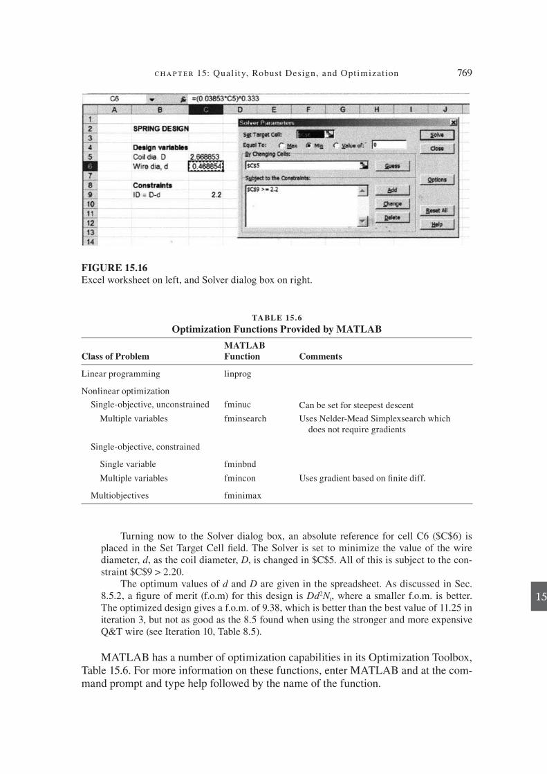
chapter 15: Qual ity, Robust Design, and Optimizat ion 769
15
Turning now to the Solver dialog box, an absolute reference for cell C6 ($C$6) is placed in the Set Target Cell ? eld. The Solver is set to minimize the value of the wire diameter, d , as the coil diameter, D , is changed in $C$5. All of this is subject to the con-straint $C$9 > 2.20.
The optimum values of d and D are given in the spreadsheet. As discussed in Sec. 8.5.2, a ? gure of merit (f.o.m) for this design is Dd 2 N t , where a smaller f.o.m. is better. The optimized design gives a f.o.m. of 9.38, which is better than the best value of 11.25 in iteration 3, but not as good as the 8.5 found when using the stronger and more expensive Q&T wire (see Iteration 10, Table 8.5).
MATLAB has a number of optimization capabilities in its Optimization Toolbox, Table 15.6. For more information on these functions, enter MATLAB and at the com-mand prompt and type help followed by the name of the function.
FIGURE 15.16
Excel worksheet on left, and Solver dialog box on right.
Class of Problem
MATLAB
Function Comments
Linear programming linprog
Nonlinear optimization
Single-objective, unconstrained
Multiple variables
fminuc
fminsearch
Can be set for steepest descent
Uses Nelder-Mead Simplexsearch which does not require gradients
Single-objective, constrained
Single variable fminbnd
Multiple variables fmincon Uses gradient based on ? nite diff.
Multiobjectives fminimax
TABLE 15.6
Optimization Functions Provided by MATLAB
die37039_ch15.indd 769 2/25/08 7:02:15 PM

770 engineering design
15
For examples in the use of these functions, see Arora 41 and Magrab. 42
Multiobjective Optimization
Multiobjective optimization refers to the solution of problems with more than one objective function. The design objectives in these problems are inherently in con-v ict. Consider a shaft loaded in torsion with the two design objectives of maximizing strength and minimizing weight (cost). As the diameter of the shaft is reduced to de-crease weight, the stress is increased, and vice versa. This is the classical problem of design trade-off . At some point in the optimization process the designer reaches a point where it is no longer possible to improve both design objectives. Such a point is referred to as a Pareto point, and the locus of these points de? nes the Pareto frontier, Fig. 15.17b.
To solve such problems, the optimization method ? nds the set of Pareto solutions. The actual decision maker can be queried for his or her preferences, and the designer can rank order the preferences.
15.8.4 Other Optimization Methods
Monotonicity Analysis
Monotonicity analysis is an optimization technique that may be applied to design problems with monotonic properties, that is, where the change in objective function and constraints steadily increases (or decreases) over the design space. This is a situa-tion that is very common in design problems. Engineering designs tend to be strongly de? ned by physical constraints. When these speci? cations and restrictions are mono-tonic in the design variables, then monotonicity analysis can often show the designer which constraints are active at the optimum. An active constraint refers to a design requirement that has a direct impact on the location of the optimum. This information can be used to identify the improvements that could be achieved if the feasible domain were modi? ed, which would point out directions for technological improvement.
Feasible domainFeasible
domain
Pareto frontier
(a) (b)
x2
x1,x2
f1, f2
x1 f1
f 2
FIGURE 15.17
Feasible domains in (a) the design variable space and (b) the objective function space with its Pareto frontier.
41. J. S . Arora , op. cit, Chap. 12.
42. E. B . Magrab , et al. An Engineer’s Guide to MATLAB, 2d ed., Chap. 13, S . Azarm , “ Optimization ,” Prentice Hall, Upper Saddle River, NJ , 2005 .
die37039_ch15.indd 770 2/25/08 7:02:16 PM

chapter 15: Qual ity, Robust Design, and Optimizat ion 771
15
The ideas of monotonicity analysis were ? rst presented by Wilde. 43 Subsequent work by Wilde and Papalambros has applied the method to many engineering prob-lems 44 and to the development of a computer-based method of solution. 45
Dynamic Programming
Dynamic programming is a mathematical technique that is well suited for the optimization of staged processes. The word dynamic in the name of this technique has no relationship to the usual use of the word to denote changes with respect to time. Dynamic programming is related to the calculus of variations and is not related to linear and nonlinear programming methods. The method is well suited for allo-cation problems, as when x units of a resource must be distributed among N activi-ties in integer amounts. It has been broadly applied within chemical engineering to problems like the optimal design of chemical reactors. Dynamic programming con-verts a large, complicated optimization problem into a series of interconnected smaller problems, each containing only a few variables. This results in a series of partial opti-mizations that requires a reduced effort to ? nd the optimum. Dynamic programming was developed by Richard Bellmann 46 the 1950s. It is a well-developed optimization method. 47
Genetic Algorithms
Genetic algorithms (GA) are a form of computational design that uses simulated biological evolution as its search strategy. Genetic algorithms are stochastic in that there are probabilistic parameters that govern the GA’s operation. GAs are also itera-tive because they involve many cycles of generating designs and checking for the best options.
Genetic algorithms mimic biological evolution. The basic idea of genetic algo-rithms is to transform the problem into one solved by evolution as de? ned in the natu-ral sciences. Under evolution by natural selection, the ? ttest (i.e., best suited to thrive in the environment) members of a population survive and produce offspring. It’s likely that the offspring inherit some of the characteristics that led to their parents’ survival. Over time, the average ? tness of a population increases as natural selection acts. The principles of genetics allow random mutation in a small percentage of the population. This is how some new characteristics arise over time.
The most unique contribution of genetic algorithms is the representation of each design as a string of binary computer code. The creation of new designs for a next
43. D. J. Wilde, Trans. ASME, Jnl. of Engr for Industry, Vol. 94, pp. 1390–94, 1975.44. P. Papalambros and D. J. Wilde, Principles of Optimal Design, 2d ed. Cambridge University Press, New York, 2000.
45. S . Azarm and P . Papalambros , Trans. ASME, Jnl. of Mechanisms, Transmissions, and Automation in
Design, Vol. 106, pp. 82–89 , 1984 . 46. R. E . Bellman , Dynamic Programming, Princeton University Press, Princeton, NJ , 1957 .
47. G. L . Nernhauser , Introduction to Dynamic Programming, John Wiley & Sons, New York , 1960 ; E. V . Denardo , Dynamic Programming Models and Applications, Prentice Hall, Englewood Cliffs, NJ , 1982 .
die37039_ch15.indd 771 2/25/08 7:02:17 PM

772 engineering design
15
generation is complex because several rules are used to mimic the action of genetic inheritance. Using binary computer code to represent designs enables computational shortcuts in manipulating designs to offset the complexity and allow iterations of tens of generations of populations of 100 designs each. Genetic algorithms are not widely used in mechanical design optimization, but their potential is so great that one expects them to increase in popularity. To ? nd more information on all aspects of genetic algorithms (e.g., research papers, MATLab codes), visit the site for the International Society for Genetic and Evolutionary Computation at www.isgec.org.
Evaluation Considerations in Optimization
We have presented optimization chiev y as a collection of computer-based math-ematical techniques. However, of more importance than knowing how to manipulate the optimization tools is knowing where to use them in the design process. In many designs a single design criterion drives the optimization. In consumer products it usu-ally is cost, in aircraft it is weight, and in implantable medical devices it is power consumption. The strategy is to optimize these “bottleneck factors” ? rst. Once the primary requirement has been met as well as possible, there may be time to improve other areas of the design, but if the ? rst is not achieved, the design will fail. In some areas of design there may be no rigid speci? cations. An engineer who designs a talk-ing, walking teddy bear can make almost any trade-off he or she wants between cost, power consumption, realism, and reliability. The designers and market experts will work together to decide the best combination of characteristics for the prod-uct, but in the end the four-year-old consumers will decide whether it is an optimal design.
15.9 DESIGN OPTIMIZATION
It has been a natural development to combine computer-aided-engineering (CAE) analysis and simulation tools with computer-based optimization algorithms. 48 Link-ing optimization with analysis tools creates CAE design tools by replacing traditional trial-and-error approaches with a systematic design-search approach. This extends the designer’s capability from being able with FEA to quantify the performance of a par-ticular design to adding information about how to modify the design to better achieve critical performance criteria.
Figure 15.18 shows a general framework for CAE-based optimal design. Start-ing with an initial design (size and shape parameters), a numerical analysis simula-tion, such as FEA, is performed on the design to compute the performance measures, such as von Mises stress, and the sensitivity of the performance measures with re-spect to the design parameters. Then an optimization algorithm computes new design
48. D. E. Smith, “Design Optimization,” ASM Handbook, Vol. 20, pp. 209–18, ASM International, Ma-terials Park, OH, 1997.
die37039_ch15.indd 772 2/25/08 7:02:17 PM

chapter 15: Qual ity, Robust Design, and Optimizat ion 773
15
parameters, and the process is continued until an optimum design is achieved. Often this is not a mathematical optimum but a set of design variables for which the objec-tive function shows appreciable improvement.
Most FEA packages offer optimization routines that integrate design simula-tion, optimization, and design-sensitivity analysis into a comprehensive design envi-ronment. The user inputs preliminary design data and speci? es acceptable variables and required constraints. The optimization algorithm generates successive models, in conjunction with remeshing routines, until it ultimately converges on an optimized design. For example, structural optimization of a turbine wheel design resulted in a 12 percent reduction in mass and a 35 percent reduction in stress.
Structural design optimization can be classi? ed into three groups: (1) size opti-mization, (2) shape optimization, and (3) topology optimization. Size optimization is the easiest and requires the least computer power. Size optimization deals with parameters that do not alter the location of nodal points in the numerical model. Examples are material properties, boundary conditions, and element properties such as plate thickness. Shape optimization deals with parameters that describe boundary po-sition in the numerical model. Since these de? ne nodal locations, shape optimization
Initial design
CAE design
Numerical
analysis
Performance
measures
Optimization
Convergence?
Optimal design
No
Yes
Sensitivity
analysis
FIGURE 15.18
General framework for CAE-based design optimization. (From D. E. Smith, ASM Handbook, Vol. 20, p. 211. Used with permission.)
die37039_ch15.indd 773 2/25/08 7:02:18 PM
774 engineering design
15
generally requires that the entire numerical model be remeshed. Shape optimization can lead to important design bene? ts, but it also can yield shapes that are dif? cult or impossible to manufacture. To avoid this situation, topology optimization is being introduced. The goal of topology optimization is to determine where to place material and where to leave it out of the structure. It is best done early in the design process when little has been decided about the design details and when design changes are most easily accommodated. 49 For example, topology optimization could help deter-mine the number and placement of holes or stiffening members. This would provide a good starting point for size optimization and shape optimization. Topology optimiza-tion packages being introduced allow the user to specify manufacturing dimensions and other design features as design constraints. They also allow cost to be considered as an optimization parameter.
15.10 SUMMARY
This chapter presents many of the modern views about design. The overarching con-cept is that quality is built into products during design. Manufacturing cannot com-pensate for errors in design. Second, we have emphasized that variability during manufacture and in service is the the challenge to a quality design. We aim for a robust design that is less sensitive to process variations and to extreme conditions in service.
Quality must be viewed as a total system from the perspective called total quality management (TQM). TQM places the customer at the center and solves problems with a data-driven approach using simple but powerful tools (see Sec. 3.7). It emphasizes continuous improvement where large changes are achieved by many small improve-ments made over time.
Statistics plays a signi? cant role in achieving quality and robustness. A control chart shows whether the variability of a process is within reasonable bounds. The pro-cess capability index C p , tells whether the selected tolerance range is easily achievable by a particular process.
New ways of looking at quality have been introduced by Taguchi. The loss func-tion provides a better way of looking at quality than the traditional upper and lower tolerance limits around a mean value. The signal-to-noise parameter (S/N) provides a powerful metric to search for design situations that minimize variability. Orthogonal experimental designs provide a useful and widely adopted methodology to ? nd the design or process conditions that are most robust.
The search for optimum conditions has been a design goal for many years. A wide selection of optimization methods is described in Sec. 15.7. The coming together of optimization routines with computer modeling methods to provide a powerful design optimization tool ends this chapter.
49. M . Chirehdast , H-C . Gea , N . Kikuchi , and P. Y . Papalambros , Jnl. of Mechanical Design, Vol. 116, pp. 997–1004 , 1994 .
die37039_ch15.indd 774 2/25/08 7:02:18 PM

chapter 15: Qual ity, Robust Design, and Optimizat ion 775
15
NEW TERMS AND CONCEPTS
Design optimization Equality constraint Genetic algorithm Golden section search Inequality constraint ISO 9000 Lattice search Loss function
Multiobjective optimization Noise factors Objective function Process capability indexQuality Quality assurance Quality control Range
Robust design Signal-to-noise ratio Six Sigma quality Statistical process control Steepest descent search Taguchi method Univariate search Upper control limit
BIBLIOGRAPHY
Quality
Bester? eld , D. H .: Total Quality Management, 3d ed., Prentice Hall, Upper Saddle River, NJ , 2003 .
Gevirtz , C. D .: Developing New Products with TQM, McGraw-Hill, New York , 1994 . Kolarik , W. J .: Creating Quality, McGraw-Hill, New York , 1995 . Summers , D. C. S .: Quality, Prentice Hall, Upper Saddle River, NJ , 1997 .
Robust Design
Ealey , L. A .: Quality by Design, 2d ed., ASI Press, Dearborn, MI , 1984 . Fowlkes , W. Y ., and C. M . Creveling : Engineering Methods for Robust Product Design,
Addison-Wesley, Reading MA , 1995 . Ross , P. J .: Taguchi Techniques for Quality Engineering, 2d ed., McGraw-Hill, New York ,
1996 . Wu , Y ., and A . Wu , Taguchi Methods for Robust Design, ASME Press, New York , 2000 .
Optimization
Arora , J. S .: Introduction to Optimum Design, 2d ed., Elsevier Academic Press, San Diego, CA , 2004 .
Papalambros , P. Y ., and D. J . Wilde : Principles of Optimal Design, 2d ed., Cambridge Univer-sity Press, New York , 2000 .
Park , G. J .: Analytic Methods for Design Practice, Spriner-Verlag, London , 2007 . Ravindran , A ., Ragsdell , K. M ., and G. V . Reklaitis , Engineering Optimization, 2d ed., John
Wiley & Sons, Hoboken, NJ , 2006 . Vanderplaats , G. N .: Numerical Optimization Techniques for Engineering Design, McGraw-
Hill, New York , 1984 .
PROBLEMS AND EXERCISES
15.1 Discuss as a class how Deming’s 14 points could be applied to higher education.
15.2 Divide into teams and use the TQM problem-solving process introduced in Sec. 4.7 to decide how to improve the quality in several of your courses (one course per team).
die37039_ch15.indd 775 2/25/08 7:02:18 PM

776 engineering design
15
15.3 Discuss the concept of quality circles. What would be involved in implementing a qual-ity circle program in industry? How could the concept be applied to the classroom?
15.4 Use the concept of statistical hypothesis testing to identify and classify the errors that can occur in quality-control inspection.
15.5 Dig deeper into the subject of control charts and ? nd some rules for identifying out- of-control processes.
15.6 For the control chart shown in Fig. 15.5, determine C p . Note: Hardness is only recorded to the nearest 0.5 RC.
15.7 A product has speci? cation limits of 120 " 10 MN and a target value of 120 MN. The standard deviation of the products coming off the process line is 3 MN. The mean value of strength is initially 118 MN, but it shifts to 122 MN and then 125 MN without any change in variability. Determine C p and C pk .
15.8 The equations in Sec. 15.4 for process capability index are for parameters that have two-sided tolerances about the target value. What if your design parameter was frac-ture toughness, K Ic . What would the equation for C p be when you are only concerned with a one-sided tolerance below the target value?
15.9 A grinding machine is grinding the root of gas turbine blades where they attach to the disk. The critical dimension at the root must be 0.450 ± 0.006 in. Thus, a blade falls out of specs in the range 0.444 to 0.456 and has to be scrapped at a cost of $120.
(a) What is the Taguchi loss equation for this situation?
(b) Samples taken from the grinder had the following dimensions: 0.451; 0.446; 0.449; 0.456; 0.450; 0.452; 0.449; 0.447; 0.454; 0.453; 0.450; 0.451
What is the average loss function for the parts made on the machine?
15.10 The weather strip that seals the door of an automobile has a speci? cation on width of 20 "4 mm. Three suppliers of weather strip produced the results shown below.
Supplier Mean width Variance s 2 C pk
A 20.0 1.778 1.0
B 18.0 0.444 1.0
C 17.2 0.160 1.0
Field experience shows that when the width of the weather strip is 5 mm below the target the seal begins to leak and about 50 percent of the customers will complain and insist that it be replaced at a cost of $60. When the strip width exceeds 25 mm door closure becomes dif? cult and the customer will ask to have the weather strip replaced. Historically, the three suppliers had the following number of parts out of spec in deliv-eries of 250,000 parts: A: 0.27%; B: 0.135%; C: 0.135%.
(a) Compare the three suppliers on the basis of loss function.
(b) Compare the three suppliers on the basis of cost of defective units.
die37039_ch15.indd 776 2/25/08 7:02:19 PM
chapter 15: Qual ity, Robust Design, and Optimizat ion 777
15
15.11 Part of the pollution control system of an automobile engine consists of a nylon tube inserted in a v exible elastomeric connector. The tubes had been coming loose, so an experimental program was undertaken to improve the robustness of the design. The ef-fectiveness of the design was measured by the pounds of force needed to pull the nylon tube out of the connector. The control factors for this design were:
A —interference between the nylon tube and the elastomer connector B —wall thickness of the elastomer connector C —depth of insertion of the tube in the connector D —the percent, by volume, of adhesive in the connector pre-dip
The environmental noise factors that conceivably could affect the strength of the bond had to do with the conditions of the pre-dip that the end of the connector was im-mersed in before the tube was inserted. There were three:
X —time the predip was in the pot 24 h and 120 h
Y —temperature of the predip 72°F and 150°F
Z —relative humidity 25% and 75%
(a) Set up the orthogonal arrays for the control factors (inner array) at three levels and the noise factors (outer array). How many runs will be required to complete the tests?
(b) The calculated S/N ratio for the pull-off force of the tube for the nine experimen-tal conditions of the control matrix are, in order: (1) 24.02; (2) 25.52; (3) 25.33; (4) 25.90; (5) 26.90; (6) 25.32; (7) 25.71; (8) 24.83; (9) 26.15. What type of S/N ratio should be used? Determine the best settings for the design parameters.
15.12 Conduct a robust design experiment to determine the most robust design of paper air-planes. The control parameters and noise parameters are given in the following table.
Control parameters
Parameter Level 1 Level 2 Level 3
Weight of paper ( A ) One sheet Two sheets Three sheets
Con? guration ( B ) Design 1 Design 2 Design 3
Width of paper ( C ) 4 in 6 in 8 in
Length of paper ( D ) 6 in 8 in 10 in
Noise parameter
Parameter Level 1 Level 2
Launch height ( X ) Standing on ground Standing on chair
Launch angle ( Y ) Horizontal to ground 45° above horizontal
Ground surface Concrete Polished tile
die37039_ch15.indd 777 2/25/08 7:02:19 PM

778 engineering design
15
All planes are launched by the same person in a closed room or hallway with no air currents. When launching a plane, the elbow must be touching the body and only the forearm, wrist, and hand are used to send the plane into v ight. Planes are made from ordinary copy paper. The class should decide on the three designs, and once this is decided, the designs will not be varied throughout the experiment. The objective func-tion to be optimized is the distance the plane v ies and glides to a stop on the v oor, measured to the nose of the plane.
15.13 We want to design a hot-water pipeline to carry a large quantity of hot water from the heater to the place where it will be used. The total cost is the sum of four items: (1) the cost of pumping the water, (2) the cost of heat lost from the pipe, (3) the cost of the pipe, (4) the cost of insulating the pipe.
(a) By using basic engineering principles, show that the system cost is
C KD
KD x D
K D K xp h m i= + ( ) + +
1 15 ln + /
where x is the thickness of insulation on a pipe of inside diameter D .
(b) If K p 5 10.0, K h 5 2.0, K m 5 1.0, and initial values of x and D are equal to 1.0, ? nd the values of D and x that will minimize the system cost. Use an alternating single-variable search.
15.14 Find the maximum value of y 5 12 x 2 x 2 with the golden section search method for an original interval of uncertainty of 0 # x # 10. Carry out the search until the difference between the two largest calculated values of y is 0.01 or less. Do the same problem us-ing the Excel Solver.
die37039_ch15.indd 778 2/25/08 7:02:20 PM

16
779
16
COST EVALUATION
16.1
INTRODUCTION
An engineering design is not complete until we have a good idea of the cost required to build the design or manufacture the product. Generally, among functionally equiva-lent alternatives, the lowest-cost design will be successful in a free marketplace. The fact that we have placed this chapter on cost evaluation toward the end of the text does not re@ ect the importance of the subject.
Understanding the elements that make up cost is vital because competition be-tween companies and between nations is C ercer than ever. The world is becoming a single gigantic marketplace in which newly developing countries with very low labor costs are acquiring technology and competing successfully with the well-established industrialized nations. Maintaining markets requires a detailed knowledge of costs and an understanding of how new technology can lower costs.
Decisions made in the design process commit 70 to 80 percent of the cost of a product. It is in the conceptual and embodiment design stages that a majority of the costs are locked into the product. Thus, this chapter emphasizes how accurate cost estimates can be made early in the design process.
Cost estimates are used in the following ways:
To provide information to establish the selling price of a product or a quotation for a good or service. To determine the most economical method, process, or material for manufacturing a product. To become a basis for a cost-reduction program. To determine standards of production performance that may be used to control costs. To provide input concerning the proC tability of a new product.
It can be appreciated that cost evaluation inevitably becomes a very detailed and “nitty-gritty” activity. Detailed information on cost analysis rarely is published
1.
2.
3.4.5.
die37039_ch16.indd 779 2/25/08 7:03:03 PM

780 engineering design
16
in the technical literature, partly because it does not make interesting reading but more important, because cost data are highly proprietary. Therefore, the emphasis in this chapter will be on the identiC cation of the elements of costs and on some of the more generally accepted cost evaluation methods. Cost estimation within a particular industrial or governmental organization will follow highly specialized and standard-ized procedures particular to the organization. However, the general concepts of cost evaluation described here will still be valid.
16.2
CATEGORIES OF COSTS
We can divide all costs into two broad categories: product costs and period costs. Product costs are those costs that vary with each unit of product made. Material cost and labor cost are good examples. Period costs derive their name from the fact that they occur over a period of time regardless of the amount (volume) of product that is made or sold. An example would be the insurance on the factory equipment or the expenses associated with selling the product. Another name for a product cost is vari-
able cost , because the cost varies with the volume of product made. Another name for period cost is ! xed cost , because the costs remain the same regardless of the volume of product made. Fixed costs cannot be readily allocated to any particular product or service that is produced.
Yet another way of categorizing costs is by direct cost and indirect cost. A direct
cost is one that can be directly associated with a particular unit of product that is manufactured. In most cases, a direct cost is also a variable cost, like materials cost. Advertising for a product would be a direct cost when it is assignable to a speciB c product or product line, but it is not a variable cost because the cost does not vary with the quantity produced. An indirect cost cannot be identiB ed with any particular prod-uct. Examples are rent on the factory building, cost of utilities, or wages of the shop D oor supervisors. Often the line between direct costs and indirect costs is fuzzy. For example, equipment maintenance would be considered a direct cost if the machines are used exclusively for a single product line, but if many products were manufactured with the equipment, their maintenance would be considered an indirect cost.
Returning to the cost classiB cations of B xed and variable costs, examples are:
Fixed costs
Indirect plant cost (a) Investment costs
Depreciation on capital investment Interest on capital investment and inventory Property taxes Insurance
(b) Overhead costs (burden) Technical services (engineering) Product design and development
1.
die37039_ch16.indd 780 2/25/08 7:03:03 PM

chapter 16: Cost Evaluat ion 781
16
Nontechnical services (ofB ce personnel, security, etc.) General supplies Rental of equipment
Management and administrative expenses (a) Share of cost of corporate executive staff (b) Legal staff (c) Share of corporate research and development staff (d) Marketing staff
Selling expenses (a) Sales force (b) Delivery and warehouse costs (c) Technical service staff
Variable costs
Materials Direct labor (including fringe beneB ts) Direct production supervision Maintenance costs Power and utilities Quality-control staff Royalty payments Packaging and storage costs Scrap losses and spoilage
Fixed costs such as marketing and sales costs, legal expense, security costs, B nan-cial staff expense, and administrative costs are often lumped into an overall category known as general and administrative expenses (G&A expenses). The preceding list of B xed and variable costs is meant to be illustrative of the chief categories of costs, but it is not exhaustive.
The way the elements of cost build up to establish a selling price is shown in Fig. 16.1. The chief cost elements of direct material, direct labor, and any other direct expenses determine the prime cost . To it must be added indirect manufacturing costs such as light, power, maintenance, supplies, and factory indirect labor. This is the fac-
tory cost . The manufacturing cost is made up of the factory cost plus general B xed expenses such as depreciation, engineering, taxes, ofB ce staff, and purchasing. The total cost is the manufacturing cost plus the sales expense. Finally, the selling price is established by adding a proB t to the total cost.
Another important cost category is working capital , the funds that must be pro-vided in addition to B xed capital and land investment to get a project started and pro-vide for subsequent obligations as they come due. It consists of raw material on hand, semiB nished product in the process of manufacture, B nished product in inventory, accounts receivable, 1 and cash needed for day-to-day operation. The working capital
2.
3.
1.2.3.4.5.6.7.8.9.
1 . Accounts receivable represents products that have been sold but for which your company has not yet been paid.
die37039_ch16.indd 781 2/25/08 7:03:04 PM

782 engineering design
16
is tied up during the life of the plant, but it is considered to be fully recoverable at the end of the life of the project.
Break-Even Point
Separating costs into B xed and variable costs leads to the concept of the break-even point (BEP), Fig. 16.2. The break-even point is the sales or production volume at which sales and costs balance. Operating beyond the BEP results in proB ts; operating below the BEP results in losses. Let P be the unit sales price ($/unit), v be the variable cost ($/unit), and f be the B xed cost ($). Q is the number of production units, or the sales volume of products sold. The gross proB t Z is given by 2
Z PQ Qv + f
At the break-even point, Q QBE
= − ( )=
PP
BEP BEP
and Z 0
Q P v f Therefore, Qf
=
−( ) = =PP v−
(16.1)
E X A M P L E 1 6 . 1 A new product has the following cost structure over one month of op-eration. Determine the break-even point.
Labor cost 2.50 $/unit Material cost 6.00 $/uunit
G & A expenses $1200 Depreciation on equuipment $5000
Factory expenses $900 Sales & ddistribution overhead $1000
Profit $1.70 $/uunit
Total variable cost, v, 2.50 6.00 8.50= + = $/unit
Direct
material
Direct
labor
Factory
expense
Prime
cost
Factory
cost
General
expense
Sales
expense
Manufacturing
cost
Total
cost
Profit
Selling
price
FIGURE 16.1 Elements of cost that establish the selling price.
2 . Gross proB t is the proB t before subtracting general and administrative expenses and taxes.
die37039_ch16.indd 782 2/25/08 7:03:04 PM
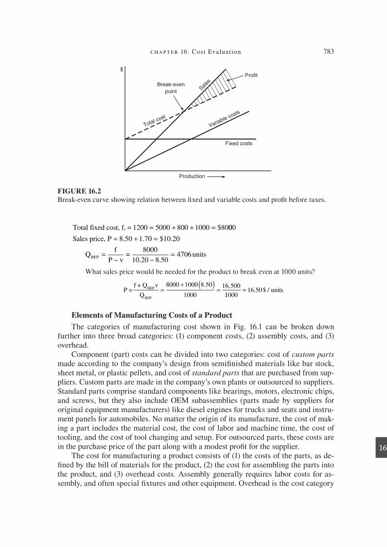
chapter 16: Cost Evaluat ion 783
16
Total fixed cost, f, 1200 5000 800 1000 $80= = + + = 000
Sales price, P 8.50 1.70 $10.20
Qf
P vBEP
= + =
=−
==−
=8000
10 20 8 504706
. .units
What sales price would be needed for the product to break even at 1000 units?
P =f + Q v
QBEP
BEP
=+ ( )
=8000 1000 8 50
1000
16 500. ,
1100016 50= . $ / units
Elements of Manufacturing Costs of a Product
The categories of manufacturing cost shown in Fig. 16.1 can be broken down further into three broad categories: (1) component costs, (2) assembly costs, and (3) overhead.
Component (part) costs can be divided into two categories: cost of custom parts made according to the company’s design from semiB nished materials like bar stock, sheet metal, or plastic pellets, and cost of standard parts that are purchased from sup-pliers. Custom parts are made in the company’s own plants or outsourced to suppliers. Standard parts comprise standard components like bearings, motors, electronic chips, and screws, but they also include OEM subassemblies (parts made by suppliers for original equipment manufacturers) like diesel engines for trucks and seats and instru-ment panels for automobiles. No matter the origin of its manufacture, the cost of mak-ing a part includes the material cost, the cost of labor and machine time, the cost of tooling, and the cost of tool changing and setup. For outsourced parts, these costs are in the purchase price of the part along with a modest proB t for the supplier.
The cost for manufacturing a product consists of (1) the costs of the parts, as de-B ned by the bill of materials for the product, (2) the cost for assembling the parts into the product, and (3) overhead costs. Assembly generally requires labor costs for as-sembly, and often special B xtures and other equipment. Overhead is the cost category
Fixed costs
Production
Variable costs
Profit
Total cost
SalesBreak-even
point
$
FIGURE 16.2 Break-even curve showing relation between B xed and variable costs and proB t before taxes.
die37039_ch16.indd 783 2/25/08 7:03:04 PM
784 engineering design
16
that accounts for those costs of manufacture that cannot be directly attributed to each unit of production. This is discussed in Sec. 16.3.
Selling Price
Manufacturing cost is an important cost element in establishing the selling price of a product. Two other cost components that must be considered in reaching the B nal cost of a product are preparing the product for shipping, and shipping it to a distribu-tion point. The selling price, which is usually the price paid by wholesalers, is the sum of these costs plus the manufacturing cost plus the proB t to the manufacturer.
Profit Selling price Total cost of product= − rrealization (16.2)
The proB t percentage (margin) is determined by the acceptance and competition in the marketplace for the product. For unique products it may be 40 to 60 percent, but 10 to 30 percent is a more typical value. A well-accepted business principle is that for a new business venture, the expected return must exceed the cost of the investment that must be made. This leads to the following simpliB ed markup pricing model. 3
Unit price =
f +viI
NN
N
y
+
(16.3)
where i 5 expected return on investment (decimal), I 5 capital investment (dollars), N y 5 payback period for investment (years), f 5 B xed cost for product (dollars), v 5 variable cost (dollars per unit), N 5 number of units sold
Wholesalers sell the product to retail outlets. The markup over wholesale cost will de-pend on the nature of the market in which the product sells. If it is a tightly controlled market, then the markup can be as great as 100 percent; if it is a highly competitive market with many “big box” stores competing with each other, then it may only be 20 percent.
16.3 OVERHEAD COST
Perhaps no aspect of cost evaluation creates more confusion and frustration in the young engineer than overhead cost. Many engineers consider overhead to be a tax on their creativity and efforts, rather than the necessary and legitimate cost it is. Over-head can be computed in a variety of ways. Therefore, you should know something about how accountants assign overhead charges.
An overhead cost 4 is any cost not speciB cally or directly associated with the pro-duction of identiB able goods or services. The two main categories of overhead costs are factory or plant overhead and corporate overhead. Factory overhead includes the
3. P. F . Ostwald and T. S . McLaren , Cost Analysis and Estimating for Engineering and Management, p. 381 , Pearson Prentice Hall, Upper Saddle River, NJ , 2004 . 4 . The term “overhead” arose in early 20 th century factories where the bosses were generally located in second-D oor ofB ces over the factory D oor.
die37039_ch16.indd 784 2/25/08 7:03:05 PM
chapter 16: Cost Evaluat ion 785
16
costs of manufacturing that are not related to a particular product. Corporate over-
head is based on the costs of running the company that are outside the manufacturing or production activities. Since many manufacturing companies operate more than one plant, it is important to be able to determine factory overhead for each plant and to lump the other overhead costs into corporate overhead. Typical cost contributions to corporate overhead are the salaries and fringe beneB ts of corporate executives, sales personnel, accounting and B nance, legal staff, R&D, corporate engineering and de-sign staff, and the operation of the corporate headquarters building.
One overhead rate may be assigned to an entire factory, but it is more common to designate different overhead rates to departments or cost centers. How the overhead is to be distributed is a management decision that is implemented by accountants.
Overhead rate OHOverhead charges
Basis= = (16.4)
Historically, the most common basis for allocating overhead charges is direct labor dollars or hours. This was chosen in the beginning of cost accounting because most manufacturing was highly labor intensive, and labor represented the major fraction of the total cost. Other bases for distributing overhead charges are machine hours, mate-rials cost, number of employees, and D oor space.
E X A M P L E 1 6 . 2 A modest-sized corporation operates three plants with direct labor and factory overhead as follows:
Cost Plant A Plant B Plant C Total
Direct labor $750,000 400,000 500,000 1,650,000
Factory overhead 900,000 600,000 850,000 2,350,000
Total 1,650,000 1,000,000 1,350,000 4,000,000
In addition, the cost of management, engineering, sales, accounting, etc., is $1,900,000. Find the corporate overhead rate based on direct labor.
Corporate overhead rate1,900,000
= =1 650 000, ,
11 15 115. %=
Then, the allocation of corporate overhead to Plant A would be $750,000(1.15) 5 $862,500
In the next example of overhead costs, we consider the use of factory overhead in de-termining the cost of performing a manufacturing operation.
E X A M P L E 1 6 . 3 A batch of 100 parts requires 0.75 h of direct labor each in the gear-cutting operation. If the cost of direct labor is $20 per h and the factory overhead is 160 percent, determine the total cost of processing a batch.
The cost of processing a batch is: 100 partss h/parts h
The facto
( )( )( ) =0 75 20 00 1500. $ . / $
rry overhead charge is: $1500 1.60
Th
( ) = $2400
ee cost of gear cutting for a batch of 100 pparts is processing cost overhead charge =+$$1500 2400 $3900. The unit cost is $39.00.+ =
die37039_ch16.indd 785 2/25/08 7:03:05 PM

786 engineering design
16
The overhead rate for a particular cost center or remanufacturing process is often expressed in dollars per direct labor hour ($/DLH). In Example 16.3, this is $2400/(100 3 0.75) 5 32$/DLH. The allocation of overhead on the basis of DLH sometimes can cause confusion as to the real cost when process improvement results in an in-crease in manufacturing productivity.
E X A M P L E 1 6 . 4 A change from a high-speed steel-cutting tool to a new coated WC tool results in halving the time for a machining operation because the new carbide tool can cut at a much faster speed without “losing its edge.” The data for the old tool and the new tool are shown in columns 1 and 2 of the following table. Because the cost of overhead is based on DLH, the cost of overhead apparently is reduced along with the cost of direct la-bor. The apparent savings per piece is 200 – 100 5 $100. However, a little reD ection will show that the cost elements that make up the overhead (supervision, tool room, mainte-nance, etc.) will not change because the DLH is reduced. Since the overhead is expressed as $/DLH, the overhead will actually double if DLH is halved. This true cost is reD ected in column (3). Thus, the actual savings per piece is 200 – 160 5 $40.
(1)
Old Tool
(2)New Tool
(Apparent Cost)
(3)New Tool
(True Cost)
Machining time, DLH $4 $2 $2
Direct labor rate, $/h $20 $20 $20
Direct labor cost $80 $40 $40
Overhead rate, $/DLH $30 $30 $60
Cost of overhead $120 $60 $120
Cost of direct labor and overhead $200 $100 $160
In many manufacturing situations, overhead allocation based on something other than DLH may be appropriate. Consider a plant whose major cost centers are a ma-chine shop, a paint line, and an assembly department. We see that it is reasonable for each cost center to have a different overhead rate in units appropriate to the function that is performed.
Cost centerEst. Factory Overhead
Est. Number of Units Overhead Rate
Machine shop $250,000 40,000 machine hours $6.25 per machine hour
Paint line 80,000 15,000 gal of paint $5.33 per gallon of paint
Assembly dept. 60,000 10,000 DLH $6.00 per DLH
The preceding examples show that the allocation of overhead on the basis of DLH may not be the best way to do it. This is particularly true of automated production systems where overhead has become the dominant manufacturing cost. In such situ-ations, overhead rates are often between 500 and 800 percent of the direct labor cost. In the limit, the overhead rate for an unmanned manufacturing operation would be inB nity.
die37039_ch16.indd 786 2/25/08 7:03:05 PM

chapter 16: Cost Evaluat ion 787
16
An advance on using DLH to determine overhead distribution is to use the pro-
ductive hour cost rate. 5 It is applied where overhead is being applied to cost centers, each consisting of common types of machines. Typically the factory will have a bud-geted amount, based on past experience, for each indirect cost category. Typical cat-egories, along with the basis for allocation, are: depreciation (MACRS value), space (sq. ft), indirect labor (DLH), utilities (HP hr), and engineering services (DLH). For example, the indirect labor pool is spread to the cost centers in proportion to each center’s fraction of the DLH multiplied by the total factory dollar budget for indirect labor. Each other category is determined in the same way, but using its appropriate allocation basis. With overhead allocated among cost centers, the machine hour cost
rate is found for each center by dividing its overhead by the budgeted hours. This is the overhead rate for work done in the cost center. Then the productive hour cost rate is the sum of the machine hour cost rate and the hourly wage rate (including beneB ts).
The productive hour cost rate provides an accurate method of allocating overhead costs when the use of production equipment plays a major role in the cost analysis. It is D exible enough to make allowance for the use of highly automated equipment. In this case, there would be a very low charge for hourly wages. If one of the cost cen-ters was an assembly area where hand assembly was being done, the depreciation and tooling charges would be negligible, while hourly wages would be signiB cant.
16.4 ACTIVITY-BASED COSTING
In a traditional cost accounting system, indirect costs are assigned to products using direct labor hours or some other unit-based measure to determine overhead cost. We have already seen (Example 16.4) where traditional cost accounting does not accu-rately represent cost when a large productivity gain has been made. Other types of distortion caused by the cost accounting system are concerned with timing; for ex-ample, the R&D costs of future products are charged to products currently being pro-duced, and more complex products will require support costs in greater proportion to their production volume. For these and other reasons a new way of assigning indirect costs called activity-based costing (ABC) has been developed. 6
Rather than assigning costs to an arbitrary reference like direct labor hours or machine hours, ABC recognizes that products incur costs by the activities that are re-quired for their design, manufacture, sale, delivery, and service. In turn, these activi-ties create cost by consuming support services such as engineering design, production planning, machine setup, and product packing and shipping. To implement an ABC system you must identify the major activities undertaken by the support departments and identify a cost driver for each. Typical cost drivers might be hours of engineer-ing design, hours of testing, number of orders shipped, or number of purchase orders written.
5. P. F . Ostwald and T. S . McLaren , op. cit. , pp. 160–63 . 6. R. S . Kaplan and R. E . Cooper , Cost and Effect: Using Integrated Cost Systems to Drive Pro! tability
and Performance, Harvard Business School Press, Boston, MA , 1998 .
die37039_ch16.indd 787 2/25/08 7:03:06 PM

788 engineering design
16
E X A M P L E 1 6 . 5 A company assembles electronic components for specialized test equip-ment. Two products A75 and B20 require 8 and 10.5 min, respectively, of direct labor, which costs $16 per hour. Product A75 consumes $35.24 of direct materials and product B20 consumes $51.20 of direct materials.
Using a traditional cost accouting system where all overhead costs are allocated to direct labor hours at a rate of $230 per DLH, the cost of a product would be:
Direct labor cost direct material cost over+ + hhead cost
For product A75: $16 8/60( ) + $ .35 24 ++ ( ) = + + =230 8 60 2 13 35 24 30 59 67 96/
For prod
. . . $ .
uuct B20: $16 10.5/60 /( ) + + ( ) =$ . $ .51 20 230 10 60 22 80 51 20 40 25 94 25. . . $ .+ + =
In an attempt to get a more accurate estimate of costs, the company turns to the ABC ap-proach. Six cost drivers are identiB ed for this manufacturing system. 7
Activity Cost Driver Rate
Engineering Hours of engineering services $60.00 per hour
Production setup Number of setups $100.00 per setup
Materials handling Number of components $0.15 per component
Automated assembly Number of components $0.50 per component
Inspection Hours of testing $40.00 per hour
Packing and shipping Number of orders $2.00 per order
The level of activity of each cost driver must be obtained from cost records.
Product A75 Product B20
Number of components 36 12
Hours of engineering services 0.10 0.05
Production batch size 50 200
Hours of testing 0.05 0.02
Units per order 2 25
In building the cost comparison between products we start with direct labor and di-rect material costs, as given above. Then we turn to ABC in allocating the overhead costs. We apply the activity level of the cost drivers to the cost rate of the driver. For example, for Product A75,
Engineering services: 0.10 h/unit $60/h× == $6.00/unit
Production setups: 100$
setupp
setup
unit unit
1
502 00= .
$
Materials handling: 36components
unit component un× =0 15 5 40.
$.
$
iit
order
order
uPacking and shipping: 2.00
$ 1
2 nnits unit= 1 00.
$
7 . In a real ABC study there would be many more activities and cost drivers than are used in this example.
die37039_ch16.indd 788 2/25/08 7:03:06 PM

chapter 16: Cost Evaluat ion 789
16
We see that by using ABC, we B nd that product B20 is less costly to produce. This shift has come entirely from changing the allocation of overhead costs from DLH to cost driv-ers based on the main activities in producing the product. B20 incurs lower overhead charges chieD y because it is a less complex product using fewer components and requiring less support for engineering, materials handling, assembly, and testing.
Using ABC leads to improved product-based decisions through more accurate cost data. This is especially important when manufacturing overhead accounts for a large fraction of manufacturing costs. By linking B nancial costs with activities, ABC provides cost information to complement nonB nancial indicators of performance like quality. The preceding data clearly show the need to reduce the number of compo-nents to lower the cost of materials handling and assembly. On the other hand, using only a single cost driver to represent an activity can be too simple. More complex factors can be developed, but at a considerable cost in the complexity of the ABC system.
ABC cost accounting is best used when there is diversity in the product mix of a company in terms of such factors as complexity, different maturity of products, pro-duction volume or batch sizes, and need for technical support. Computer-integrated manufacturing is a good example of a place where ABC can be applied because it has such high needs for technical support and such low direct labor costs.
There is more work in using ABC than traditional cost accounting, but this is partly compensated by the use of computer technology to accumulate the cost data. A big advantage of ABC is that when the system is in place it points to those areas of indirect cost where large savings could be made. Thus, ABC is an important compo-nent of a total quality management program aimed at process improvement and cost reduction.
16.5 METHODS OF DEVELOPING COST ESTIMATES
The methods to develop cost evaluations fall into three categories: (1) analogy, (2) parametric and factor methods, and (3) methods engineering.
Comparison of the Two Products on Activity-Based Costing
A75 B20
Direct labor 2.13 2.80
Direct materials 35.24 51.20
Engineering 6.00 3.00
Production setups 2.00 0.50
Materials handling 5.40 1.80
Assembly 18.00 6.00
Testing 2.00 0.80
Packing and shipping 1.00 0.80
$71.77 $66.90
die37039_ch16.indd 789 2/25/08 7:03:06 PM

790 engineering design
16
16.5.1 Analogy
In cost estimation by analogy, the future costs of a project or design are based on past costs of a similar project or design, with due allowance for cost escalation and techni-cal differences. The method therefore requires a database of experience or published cost data. This method of cost evaluation commonly is used for feasibility studies of chemical plants and process equipment. 8 When cost evaluation by analogy is used, future costs must be based on the same state of the art. For example, it would be valid to use cost data on a 777 jet transport aircraft to estimate costs for a larger 777, but it would not be correct to use the same data to predict the cost of the Boeing 787 because the main structures have changed from riveted aluminum construction to autoclave-bonded polymer-graphite B ber construction.
A concern with determining cost by analogy is to be sure that costs are being evaluated on the same basis. Equipment costs often are quoted FOB (free on board) the manufacturer’s plant location, so delivery cost must be added to the cost estimate. Costs sometimes are given for the equipment not only delivered to the plant site but also installed in place, although it is more usual for costs to be given FOB some ship-ping point.
16.5.2 Parametric and Factor Methods
In the parametric or statistical approach to cost estimation, techniques such as regres-sion analysis are used to establish relations between system cost and key parameters of the system, such as weight, speed, and power. This approach involves cost estima-tion at a high level of aggregation, so it is most helpful in the problem deB nition stage of conceptual design. For example, the cost of developing a turbofan aircraft engine might be given by
C x x= 0 139371
0 7435
2
0 0775. . .
where C is in millions of dollars, x 1 is maximum engine thrust, in pounds, and x 2 is the number of engines produced by the company. Cost data expressed in this em-pirical form can be useful in trade-off studies in the concept design phase. Parametric cost studies are often used in feasibility studies of large military systems. One must be careful not to use models of this type outside the range of data for which they apply.
Factor methods are related to parametric studies in that they use empirical rela-tionships based on cost data to B nd useful predictive relationships. In Sec. 13.9 we presented a factor method for determining the unit manufacturing cost of a part.
C VC P C C C Cu mv c mp c s ft
= + × × ×( ) (16.5)
where Cu is the manufacturing cost to make one unit of a partV is the volume of the part Cmv is the material cost per unit volume
8. M. S . Peters , K. D . Timmerhaus , and R. E . West , Plant Design and Economics for Chemical Engi-
neers, 5 th ed., McGraw-Hill, New York , 2003 .
die37039_ch16.indd 790 2/25/08 7:03:07 PM

chapter 16: Cost Evaluat ion 791
16
Pc is the basic cost to process an ideal shape by a particular processCmp is a cost factor that indicates the relative ease with which a material can
be shaped in a particular processCc is a relative cost associated with shape complexityCs is a relative cost associated with achieving minimy section thicknessCft is the cost of achieving a speciB ed surface B nish or tolerance.
It is important to understand that equations based on cost factors are not just made up in a haphazard fashion. Basic physics and engineering logic are carried as far as pos-sible before employing empirical analysis of data. Equation (16.5) is aimed at estimat-ing the cost to make a part in the conceptual design phase when many of the details of the features of the part have not been established. Its goal is to use part cost as a way of selecting the best process to make the part by including more design details than are included in the model for manufacturing cost described in Sec. 13.4.6. Equa-tion (16.5) recognizes that material cost is often the main cost driver in part cost, so it separates this factor from those associated with the process. Here the cost equation introduces P c , the basic processing cost for an “ideal shape.” This factor aggregates all of the costs of production (labor, tooling, capital equipment, overhead) as a function of the production volume. Note that for a speciB c company, P c could be decomposed into an equation representing its actual cost data. The factors in the parentheses are all factors that increase the cost over the ideal case. 9 Of these, shape complexity and tolerances (surface B nish) have the greatest effect.
Models for developing cost for manufacturing use physics-based principles to de-termine such process parameters as the forces, D ow rates, or temperatures involved. Eventually empirical cost factors are needed when dealing with process details. For example, the number of hours for machining a metal mold to be used in injection molding is given by 10 M 5 5.83( x i 1 x o )
1.27 where x i and x o are contours of the inner and outer surfaces of the mold, respectively, and in turn, are given by xi or xo 5 0.1 NSP where NSP is the number of surface patches or sudden changes in slope or curva-ture of the surface.
Factor methods of cost evaluation are used for estimating costs in the early stages of embodiment design and are employed in the concurrent costing software described in Sec. 13.9.
16.5.3 Detailed Methods Costing
Once the detailed design is completed and the B nal detailed drawings of the parts and assemblies have been prepared, it is possible to prepare a cost evaluation to 5 per-cent accuracy. This approach is sometimes called methods analysis or the industrial engineering approach. The cost evaluation requires a detailed analysis of every op-eration to produce the part and a good estimate of the time required to complete the
9 . Building a model by starting with an ideal case and degrading it with individual factors is a common approach in engineering model building. In Sec. 12.3.4 we started with an ideal endurance limit and re-duced its value by applying factors for stress concentration, diameter, and surface B nish. 10. G . Boothroyd , P . Dewhurst , and W . Knight , Product Design for Manufacture and Assembly, 2d ed., pp. 362–64 , Marcel Dekker, New York , 2002 .
die37039_ch16.indd 791 2/25/08 7:03:07 PM

792 engineering design
16
operation. A similar method is used to determine the costs of buildings and civil en-gineering projects. 11
At the outset of developing the cost estimate, the following information should be available:
Total quantity of product to be produced Schedule for production Detailed drawings and/or CAD B le Bill of materials (BOM)
In complicated products the bill of materials may be several hundred lines. This makes it important that a system be in place to keep track of all parts and make sure none are left out of the cost analysis. 12 The BOM should be arranged in layers, start-ing with the assembled product, then the B rst layer of subassemblies, then the subas-semblies feeding into this layer, all the way down to the individual parts. The total number of a given part in an assembled product is the number used at the lowest level multiplied by the number used at each other level of assembly. The total number of each part to be made or purchased is the number per product unit times the total num-ber of products to be produced.
Detailed methods costing analysis is usually prepared by a process planner or a cost engineer. Such a person must be very familiar with the machines, tooling, and processes used in the factory. The steps to determine cost to manufacture a part are:
Determine the material costs . Since the cost of material makes up 50 to 60 percent of the cost of many products, this is a good place to start.
MtCmC
f=
−( )M
1 (16.6)
where CM 5 cost of material in $/lbm 5 weight of material, lbf 5 fraction of material that ends up as scrap
Sometimes the cost of material is measured on a volume basis, and in other instances, as when machining bar stock, it might be measured per foot. Issues concerning the cost of materials were discussed in Sec. 11.5.
It is important to account for the cost of material that is lost in the form of scrap. Most manufacturing processes have an inherent loss of material. Sprues and risers that are used to introduce molten material into a mold must be removed from castings and moldings. Chip generation occurs in all machining processes, and metal stamp-ing leaves unused sheet scrap. While most scrap materials can be recycled, there is an economic loss in all cases.
Prepare the operations route sheet. The route sheet is a sequenced list of all op-erations required to produce the part. An operation is a step in the process se-
●
●
●
●
1.
2.
11. Historical cost data is published yearly by R. S. Means Co. and in the Dodge Digest of Building
Costs . Also see P. F . Ostwald , Construction Cost Analysis and Estimating, Prentice Hall, Upper Saddle River, NJ , 2001 . 12. P. F . Ostwald , Engineering Cost Estimating, 3d ed., pp. 295–97 , Prentice Hall, Upper Saddle River, NJ , 1992 .
die37039_ch16.indd 792 2/25/08 7:03:08 PM

chapter 16: Cost Evaluat ion 793
16
quence, deB ned as all the work done on a machine or workstation. For example, an operation on an engine lathe might be to face the end of a bar, then rough turn the diameter to 0.610 in. and B nish machine to 0.600. The process is the sequence of operations from the time the workpiece is taken from inventory until it is com-pleted and placed in B nished goods inventory. Part of developing the route sheet is to select the actual machine in the shop to perform the work. This is based on availability, the capacity to deliver the necessary force, depth of cut, or precision required by the part speciB cation.
Determine the time required to carry out each operation . Whenever a new part is B rst made on a machine, there must be a setup period during which old tooling is taken out and new tooling is installed and adjusted. Depending on the process, this can be a period of minutes or several days, but two hours is a more typical setup time. Each process has a cycle time, which consists of loading the workpiece into the machine, carrying out the operation, and unloading the workpiece. The pro-cess cycle is repeated many times until the number of parts required for the batch size has been made. Often there is a downtime for shift change or for maintenance on the machine or tooling.
Databases of standard times to perform small elements of typical operations are available. 13 Computer software with databases of operation times and cost cal-culation capability are available for most processes. If the needed information can-not be found in these sources, then carefully controlled time studies must be made. 14 A sampling of standard times for elements of operations is given in Table 16.1.
An alternative to using standard times for operation elements is to calcu-late the time to complete an operation element with a physical model of the pro-cess. These models are well developed for machining processes 15 and for other manufacturing processes. 16 An example of the use of this method for metal cutting is given in Sec. 16.12.1.
3.
TABLE 16.1
A Sampling of Cycle-Time Elements
Operation Element Minutes
Set up a lathe operation 78
Set up a drilling B xture 6
Brush away chips 0.14
Start or stop a machine tool 0.08
Change spindle speed 0.04
Index turret on turret lathe 0.03
13. P. F . Ostwald , AM Cost Evaluator, 4 th ed., Penton Publishing Co., Cleveland, OH , 1988 ; W . Winchell , Realistic Cost Estimating for Manufacturing, 2d ed., Society of Manufacturing Engineers, Dearborn, MI , 1989 .
14. B . Niebel and A . Freivalds , Methods, Standards, and Work Design, 11 th ed., McGraw-Hill, New York , 2003 .
15. G . Boothroyd and W. A . Knight , Fundamentals of Machining and Machine Tools, 2d ed., Chap. 6, Marcel Dekker, New York , 1989 . 16. R. C . Creese , Introduction to Manufacturing Processes and Materials, Marcel Dekker, New York , 1999 .
die37039_ch16.indd 793 2/25/08 7:03:08 PM

794 engineering design
16
Convert time to cost. The times for each element in each operation are added to B nd the total time to complete each operation of the process. Then the time is multiplied by the fully loaded wage rate ($/h) to give the cost of labor. A typical product will require parts made by different processes, and some parts purchased rather than made in-house. Typically, different labor rates and overhead rates pre-vail in different cost centers of the factory.
E X A M P L E 1 6 . 6 A ductile cast iron V-belt pulley driven from a power shaft is made in a batch of 600 units. Its shape is similar to the object in the bottom left corner of category A1 in Fig. 13.18. The material cost is $50.00 per unit. Table 16.2 gives estimates of labor hours, labor rates, and overhead charges. Determine the unit product cost.
The estimates of the standard costs for the elements of each operation give the cycle time per 100 units given in column (2). In a similar way the setup costs for a batch are estimated in column (1) for each cost center. Multiplying (2) by 6 (the batch size is 600) plus adding in the setup cost gives the time to produce a batch of 600 units. With this and the wage rate (4), we determine the batch labor cost, column (5). The overhead cost for each cost center, based on a batch of 600 units, is given in (6). Adding (5) and (6) gives all of the in-house costs for that batch. These costs are placed on a per-unit basis in
4.
TABLE 16.2
Process Plan for Ductile Iron Pulley (Batch Size 600 Units)
Cost Center Operation
(1) Setup Time
H
(2) Cycle Time
h/100 units
(3) Time to Finish
Batch, h
(4) Wage Rate $/h
(5) Batch Labor Cost
(6) Batch Over-head
(7) Labor & Overhead Per Batch
(8) Unit Cost
Outsource Purchase 600 units, rough castings, part no. 437837
$50.00
Machine shop—lathe
Total costs for operation 2.7 35 212.7 32.00 $6806 $7200 $14,006 $23.34
1. Machine faces
2. Machine V-groove in OD
3. Rough machine hub
4. Finish machine ID of bore
Machine Shop—drills
1. Drill and tap 2 holes for set screws 0.1 5 30.1 28.00 $843 $1050 $1893 $3.15
Finishing Dept.
Total cost for operation 6.3 12.3 80.1 18.50 $1482 $3020 $4502 $7.50
1. Sand blast
2. Paint
3. Install 2 set screws 0.06
Totals 9.1 52.3 322.9 $9131 $11,616 $20,401 $84.05
die37039_ch16.indd 794 2/25/08 7:03:08 PM

chapter 16: Cost Evaluat ion 795
16
(8). Note that the unit cost of $50.00 for the rough casting that was purchased from an outside foundry includes the overhead costs and proB t for that company. The unit costs for the completed part developed in Table 16.2 do not include any proB t, since that will be determined for the entire product for which the pulley is only one part.
Developing costs by an aggregated method is a lot of work, but computer databases and calculation aids make it much less of an onerous task than in the past. As already noted, this cost analysis requires a detailed process plan, which cannot be made un-til decisions on all of the design features, tolerances, and other parameters have been made. The chief drawback, then, is if a part cost turns out too high it may not be pos-sible to make design changes to correct the problem. As a result, considerable effort is being given to cost methods that are capable of determining and controlling costs as the design process is being carried out. This topic, target costing, is discussed in Sec. 16.9.
16.6 MAKE-BUY DECISION
One of the uses of a detailed cost evaluation method such as was described in Ex-ample 16.6 is to decide whether it is less costly to manufacture a part in-house than to purchase it from an outside supplier. In that example, where the rough casting was bought from an outside foundry, it was decided that the volume of cast parts that will be used by the manufacturer does not justify the cost of equipping a foundry and hir-ing the expertise to make quality castings.
The parts that go into a product fall into three categories related to whether they should be made in-house or purchased from suppliers.
Parts for which there is no in-house process capability obviously need to be pur-chased from suppliers.
Parts that are critical to the quality of the product, involve proprietary manufactur-ing methods or materials, or involve a core technical competency need to be made in-house.
Parts other than those in the previous categories, the majority of parts, offer no compelling reason to either use in-house manufacture or purchase from a supplier. The decision is usually based on which approach is least costly to obtain quality parts. Today the make-buy decision is being made not just with respect to suppli-ers in the vicinity of the manufacturer’s plant, but in locations anywhere in the world where low-cost labor and manufacturing skill exist. This phenomenon of off-
shoring is made possible by rapid communication via the Internet and cheap water transportation with container ships. It has led to a boom in low-cost manufacturing of consumer goods in China and elsewhere in Asia.
Many factors other than cost enter into a make-buy decision.
Advantages of Outsourcing
Lower cost of manufacture provides lower prime costs (materials and labor), espe-cially with overseas suppliers.
●
●
●
●
die37039_ch16.indd 795 2/25/08 7:03:09 PM

796 engineering design
16
Suppliers can provide special expertise in design and manufacturing that the prod-uct developer may not have.
Outsourcing provides increased manufacturing D exibility due to reduction in B xed costs. This lowers the breakeven point for a product.
Manufacturing in a foreign country may result in access to a foreign market for the product.
Disadvantages of Outsourcing
Outsourcing results in a loss of in-house design and manufacturing knowledge that is transferred to the supplier, and maybe to your competitors.
It is more difB cult to improve design for manufacture when in-house manufactur-ing capability is gone.
Possible unsatisfactory quality In offshoring the supply chain is much longer. There is always a danger of delays in supply due to delay in gaining entry into port, strikes on the docks, and severe weather in transit.
Also, offshoring may present such issues as currency exchange, communication in a different language and business culture, and the added expense in coordinating with an external supplier.
16.7 MANUFACTURING COST
Manufacturing costs begin to be determined in embodiment design as design details become B rmed up. The methodology developed by Swift and coworkers at the Uni-versity of Hull, and described in Sec. 13.9, and the Concurrent Costing software de-scribed in Example 13.7, are good examples of the tools available to make an early estimate of manufacturing cost.
Detailed manufacturing cost evaluation requires considerable speciB city in di-mensions, tolerances, materials, and process planning. See Example 16.6 for a sim-ple example. This type of analysis cannot be done before detail design is complete and there is a bill of materials. Most commonly this is done in a process planning step that follows detail design. However, with the computerization of the costing process, it is becoming easier to move this process to a point earlier in the design process.
A basic equation for the cost of manufacturing a part was given in Sec. 13.4.6:
CmC
f
C
n
kC
n n
C
tq
Cu
M L T c
wo
OH=−( ) + + +
+
1
1
& & &L nn (16.7)
This equation estimates the unit manufacturing cost for a part in terms of the material cost, labor cost, tooling cost, equipment cost, and overhead. See Sec. 13.4.6 for deB ni-tion of terms and units. Equation (16.7) is used in the conceptual or early embodiment phase of design to select a process for making a part on the basis of relative cost. The
●
●
●
●
●
●
●
●
die37039_ch16.indd 796 2/25/08 7:03:09 PM

chapter 16: Cost Evaluat ion 797
16
equation requires no information about part features, but depends on process informa-tion that is usually available in general terms.
However, as seen in Example 16.6, when detailed cost estimates are made by ag-gregating the cost of operation elements, the accuracy of predictions is greatly in-creased, and the equation for unit product cost is more straightforward.
C C C OHu M L F
= + + (16.8)
where C M is the material cost per unit, C L is the labor cost per unit, and OH F is the factory overhead.
The material cost includes the purchase cost of standard components, like bear-ings and gears, and the cost of raw material (bar stock, castings, etc.) from which the components are manufactured.
CVc
fOH B OH
M
m
m b=
−+
+ +( )ρ
1 (16.9)
where V is the volume of the part, c m is the material cost per unit weight, r is the ma-terial density, and f is the fraction of scrap. OH m is a material overhead to account for the procurement, inspection, storage, interest on this inventory, and material handling costs. B is the purchase cost of components and OH b is the overhead on B .
The labor costs C L depend on the time to complete all operations to make the part, tp 5 ! t0 . An overhead on labor cost is sometimes charged. OHL is made up of time spent changing tools, lubricating, and similar activities, plus a nonproductive time allowance for time spent resting and waiting for parts.
C t c C OHL p L su L
= + + (16.10)
where c L is the direct labor wage rate, $/h, and C su is the total cost of machine setup for the process.
When overhead is broken out with respect to material cost and labor cost, as has been done in Eqs. (16.9) and (16.10), one must be careful not to double count overhead in Eq. (16.8). The accountants preparing the lists of indirect costs need to be aware of what charges, typically factory supervision and administration, go there, and what are charged to materials and labor. Typically in our examples we do not go to that level of detail.
16.8 PRODUCT PROFIT MODEL
An equation for estimating the cost to develop, manufacture, and market a consumer product is given in Eq. (16.11). Note that this equation does not give the cost for one unit of product, as we have typically done in this chapter, but rather calculates the product cost to produce a quantity of product units NP.
C N C C OH T M OH Cp p M L F c D
= + +( ) + + + + (16.11)
die37039_ch16.indd 797 2/25/08 7:03:09 PM

798 engineering design
16
The bracketed terms in Eq. (16.11) are the same as in Eq. (16.8) and are variable costs. The other terms in Eq. (16.11) are B xed but not necessarily constant costs. T is the one-time costs for equipment and tooling. M is the marketing and sales costs, OH C is corporate overhead costs, and C D is the cost for developing the product and providing modest product updates.
We can now develop a simple proB t model for the product.
( ) ( ) (1 Net sales number of units sold sales= × price
Cost of product sold number of
)
( ) (2 = units sold unit cost
Gross margin
) ( )
( ) (
×=3 11 2
4
) ( )
( )
− = −Net sales Cost of product sold
OOperating expenses tooling marketing corp.= + + OH development
Operating income (profi
+( )5 tt) gross margin operating expenses= − = −( ) ( )3 4
PPercentage profit profit/net sales= ×( ) 100
(16.12)
(16.13)
(16.14)
(16.15)
(16.16)
(16.17)
Unit cost will be arrived at from Eq. (16.11) and by the methods discussed in Sec. 16.7. The number of units sold will be estimated by the marketing staff. Other costs will be provided by cost accounting or historical corporate records.
Note that the proB t determined by the proB t model is not the “bottom line” net proB t found on the income statement of the annual report of a company. The net proB t is the aggregate proB t of many product development projects. To get from the operating income of a company to its net proB t, many additional deductions must be made, the chief of which are the interest on borrowed debt and federal and state tax payments.
It is convenient to build the proB t model with a computer-based spreadsheet pro-gram. Figure 16.3 shows a typical cost projection for a consumer product. Note that the sales price is projected to decline slightly as other competitors come into the mar-ket, but the sales volume is expected to increase over most of the life of the product as it gains acceptance through use by customers and advertising. This results in a nearly constant gross margin over the life of the product.
The development cost is broken out as a separate item in Fig. 16.3. The product was developed in a two-year period spread over 2002 to 2004. After that a modest an-nual investment was made in small improvements to the product. It is encouraging to see that the product was an instant hit and recovered its development cost in 2004, the year it was introduced to the market. This is a strong indication that the product de-velopment team understood the needs of the customer and satisB ed them with its new product.
Considerable marketing and sales activity began the year of product introduc-tion and are planned to continue at a high level throughout the expected life of the product. This is a reD ection of the competition in the marketplace and the recognition that a company must be aggressive in placing its products before the customer. The “other” category in the spreadsheet mostly comprises factory and corporate overhead charges.
die37039_ch16.indd 798 2/25/08 7:03:10 PM

16
799
20
02
$7
50
,00
0$
1,5
00
,00
0
$1
80
.00
$1
78
.00
$1
75
.00
$1
73
.00
$1
70
.00
$1
68
.00
$1
65
.00
$1
8,1
50
,00
0
$1
0,1
20
,00
0
$8
,03
0,0
00
$2
50
,00
0$
2,3
59
,50
0$
2,1
78
,00
0
$4
,78
7,5
00
$3
,24
2,5
00
$2
4,8
70
,00
0
17
.87
%
44
.24
%
$9
2.0
0
11
0,0
00
$2
0,1
60
,00
0
$1
1,0
40
,00
0
$9
,12
0,0
00
$2
50
,00
0$
2,6
20
,80
0$
2,4
19
,20
0
$5
,29
0,0
00
$3
,83
0,0
00
$2
1,6
27
,50
0
19
.00
%
45
.24
%
$9
2.0
0
12
0,0
00
$2
2,4
90
,00
0$
22
,10
0,0
00
$1
1,9
60
,00
0
$1
0,1
40
,00
0
$2
,87
3,0
00
$2
,65
2,0
00
$5
,77
5,0
00
$4
,36
5,0
00
$1
7,7
97
,50
0
19
.75
%
52
50
,00
0
45
.88
%
$9
2.0
0
$1
2,0
90
,00
0
$1
0,4
00
,00
0
$2
50
,00
0$
2,9
23
,70
0$
2,6
98
,80
0
$5
,87
2,5
00
$4
,52
7,5
00
$1
3,4
32
,50
0
20
.13
%
$9
3.0
00
13
0,0
00
13
0,0
00
$2
1,0
00
,00
0
$1
1,2
80
,00
0
$9
,72
0,0
00
$3
50
,00
0$
2,7
30
,00
0$
2,5
20
,00
0
$5
,60
0,0
00
$4
,12
0,0
00
$8
,90
5,0
00
19
.62
%
46
.29
%4
6.2
4%
$9
4.0
0
12
0,0
00
$1
9,5
80
,00
0
$9
5.0
0
11
0,0
00
$1
8,0
00
,00
0
$9
,60
0,0
00
$1
0,4
50
,00
0
$9
,13
0,0
00
$3
50
,00
0$
2,5
45
,40
0$
2,3
49
,60
0
$5
,24
5,0
00
$3
,88
5,0
00
$4
,78
5,0
00
19
.84
%
46
.63
%$
8,4
00
,00
0
$7
50
,00
0$
2,3
40
,00
0$
2,1
60
,00
0
$5
,25
0,0
00
$3
,15
0,0
00
$9
00
,00
0
17
.50
%
46
.67
%
$9
6.0
0
10
0,0
00
$1
,50
0,0
00
($1
,50
0,0
00
)
($2
,25
0,0
00
)
$7
50
,00
0
($7
50
,00
0)
($7
50
,00
0)
Sa
les P
rice
Un
it S
ale
s
Ne
t S
ale
s
Co
st
of
Pro
du
ct
so
ld
Gro
ss M
arg
in (
$)
De
ve
lop
me
nt
Co
st
Ma
rke
tin
g
Oth
er
To
tal O
pe
ratin
g E
xp
en
se
Op
era
tin
g I
nco
me
(P
rofit)
Op
In
co
me
(%
)
Cu
mu
lative
Op
In
co
me
Gro
ss M
arg
in (
%)
Un
it C
ost
20
03
20
04
20
05
20
06
Ye
ar
20
07
20
08
20
09
20
10
Cu
mu
lative
Sa
les
Cu
mu
lative
Gro
ss M
arg
in
Cu
mu
lative
Op
In
co
me
Ave
rag
e %
Gro
ss M
arg
in
Ave
rag
e %
Op
In
co
me
$1
41
,48
0,0
00
$6
4,9
40
,00
0
$2
4,8
70
,00
0
45
.90
%
17
.58
%
FIGURE 16.3 Cost projections for a consumer product.
die37039_ch16.indd 799 2/25/08 7:03:10 PM

800 engineering design
16
Trade-off Studies
The four key objectives associated with developing a new product are:
Bringing the cost of the product under the agreed-upon target cost. Producing a quality product that exceeds the expectation of the customer. Conducting an efB cient product development process that brings the product to market, on schedule.
Completing the development process within the approved budget for the product.
A product development team must recognize that not everything will go smoothly during the development process. There may be delays in the delivery of tooling, costs for outsourced components may increase because of higher fuel costs, or several parts may not interface according to speciB cation. Whatever the reason, when faced with issues such as these, it is helpful to be able to estimate the impact of your plan to B x the problem on the proB tability of your product. This is done by creating trade-off decision rules using the spreadsheet cost model.
Figure 16.3 represents the baseline proB t model if everything goes according to plan. Other cost models can easily be determined for typical shortfalls from plan.
A 50% cost overrun in development cost. A 5% cost overrun in unit cost. A 10% reduction in sales due to poor performance and customer acceptance. A 3-month delay in introducing the product into the marketplace.
Table 16.3 shows the impact on the cumulative operating income as a result of these changes from the baseline condition.
The trade-off rule of thumb is based on the assumption that changes are linear and each shortfall is independent of the others. For example, if a 10 percent decrease in sales causes a $2,957,000 reduction in cumulative operating proB t, then a 1 percent decrease in sales will decrease operating proB t by $295,700.
Note that the trade-off rules apply only to the particular case under study. They are not universal rules of thumb.
●
●
●
●
●
●
●
●
TABLE 16.3
Trade-Off Decision Rules Based on Deviation from Baseline Conditions
Type of ShortfallBaseline
Oper. IncomeReduced
Oper. IncomeCumulative
Impact on Pro t Rule of Thumb
50% development cost overrun
$24,870,000 $23,370,000 2$1,500,000 $30,000 per %
5% overrun on product cost
$24,870,000 $21,043,000 2$3,827,000 $765,400 per %
10% reduction in sales due to performance issues
$24,870,000 $21,913,000 2$2,957,000 $295,700 per %
3-month delay in product introduction to market
$24,870,000 $23,895,000 2$957,000 $975,000 per %
die37039_ch16.indd 800 2/25/08 7:03:10 PM
chapter 16: Cost Evaluat ion 801
16
E X A M P L E 1 6 . 7 An engineer estimated that a savings of $1.50 per unit could be made by eliminating the balancing operation on the fan of the product for which data is given in Table 16.3. However, marketing estimated there would be a 5 percent loss in sales due to increased vibration and noise of the product. Use the trade-off rules to decide whether the cost saving is a good idea.
Potential benefit: The unit cost is $96.00. The percentage saving is 1.50/96 = 0.0156 = 1.56%
1.56 per 1% change in unit× $ ,765 400 cost( ) = $ , ,1 194 000
Potential cost: 5 $295,700 = $1,478,500.×
BeneB t/cost is close but says that the potential cost in lost sales outweighs the savings. On the other hand, the estimate of lost sales of 5 percent is just an educated guess. One strat-egy might be to ask the engineer to do the cost saving estimate in greater detail, and if the cost saving holds up, make a trial lot that are sold in a limited geographic area where complaints and returns could be closely monitored. However, before doing this the prod-uct made without fan balancing needs to be carefully studied for noise and vibration with regard to OSHA requirements.
16.8.1 Pro t Improvement
Three strategies commonly used to achieve increased proB ts are: (1) increased prices, (2) increased sales, (3) and reduced cost of product sold. Example 16.8 shows the impact of changes in these factors on the proB t using the proB t model described by Eqs. (16.11) to (16.17).
E X A M P L E 1 6 . 8 Case A is the current distribution of cost elements for the product. Case B shows what would happen if price competition would allow a 5 per-
cent increase in price without loss in units sold. The increased income goes right to the bottom line.
Case C shows what would happen if sales were increased by 5 percent. There would be a 5 percent increase in the four cost elements, while unit cost remains the same. Costs and proB ts rise to the same degree and percentage proB t remains the same.
Case D shows what happens with a 5 percent productivity improvement (5 percent decrease in direct labor) brought about by a process-improve-ment program. The small increase in overhead results from the new equip-ment that was installed to increase productivity. Note that the proB t per unit has increased by 10 percent.
Case E shows what happens with a 5 percent decrease in the cost of mate-rials or purchased components. About 65 percent of the cost content of this product is materials. This cost reduction could result from a design modiB cation that allows the use of a less expensive material or eliminates a purchased component. In this case, barring a costly development program, all of the cost savings goes to the bottom line and results in a 55 percent increase in the unit proB t.
die37039_ch16.indd 801 2/25/08 7:03:11 PM

802 engineering design
16
Case A Case B Case C Case D Case E
Sales Price $100 $105 $100 $100 $100
Units Sold 100 100 105 100 100
Net sales $10,000 $10,500 $10,500 $10,000 $10,000
Direct labor $1,500 $1,500 $1,575 $1,425 $1,500
Materials $5,500 $5,500 $5,775 $5,500 $1,225
Overhead $1,500 $1,500 $1,575 $1,525 $1,500
Cost of product sold $8,500 $8,500 $8,925 $8,450 $8,225
Gross margin $1,500 $2,000 $1,575 $1,550 $1,775
Total operating expenses $1,000 $1,000 $1,050 $1,000 $1,000
Pretax proB t $500 $1,000 $525 $550 $775
Percentage proB t 5% 9.5% 5% 5.5% 7.75%
A fourth proB t improvement strategy, not illustrated by the example, is to upgrade the mix of products made and sold by the company. With this approach, greater emphasis is given to products with higher proB t margins while gradually phasing out the product lines with lower proB t margins.
16.9 REFINEMENTS TO COST ANALYSIS METHODS
Several reB nements to cost estimating methods have appeared over the years aimed at giving more accurate cost evaluations. In this section we discuss (1) adjustments for cost inD ation, (2) relationships between product or part size and cost, and (3) reduction in manufacturing costs because of learning.
16.9.1 Cost Indexes
Because the purchasing power of money decreases with time, all published cost data are out of date. To compensate for this, cost indexes are used to convert past costs to current costs. The cost at time 2 is the cost at time 1 multiplied by the ratio of the cost indexes.
C C2 1
=
Index @ time 2
Index @ time 1 (16.18)
The most readily available cost indexes are:
Consumer Price Index (CPI)—gives the price of consumer goods and services Producer Price Index (PPI)—measures the entire market output of U.S. producers of goods. The Finished Goods Price Index of the PPI is roughly split between du-
●
●
die37039_ch16.indd 802 2/25/08 7:03:11 PM

chapter 16: Cost Evaluat ion 803
16
rable goods (not in the CPI) and consumer goods. No services are measured by the PPI. Both the CPI and PPI are available at www.bls.gov.
The Engineering News Record provides indexes on general construction costs. The Marshall and Swift Index, found on the last page of Chemical Engineering magazine, provides an index of industrial equipment costs. The same magazine publishes the Chemical Engineering Plant Equipment Index, which covers equip-ment such as heat exchangers, pumps, compressors, piping, and valves.
Many trade associations and consulting groups also maintain specialized cost indexes.
E X A M P L E 1 6 . 9 An oilB eld diesel engine cost $5500 when it was purchased in 1982. What did it cost to replace the diesel engine in 1997?
C CI
I1997 1982
1997
1982
55001156 8
121 8=
=
.
.
= ( ) =5500 1 29 7095. $
What did it cost to replace the engine in 2006 if the ! nished goods price index for oil and gas B eld machinery was 210.3?
C C2006 1997
210 3
156 87095 1 34 951=
= ( ) =.
.. $ 66
We see there was an average increase in price of 1.9 percent over the B rst 15 years, and a 3.8 percent yearly average over the last 9 years. This is a reD ection of the rapid accel-eration of oil and gas business in the recent past. Similar calculations for the automobile parts business would see hardly any price increase since 1997, an indication of the B erce competition in this relatively stagnant market.
You should be aware of some of the pitfalls inherent in using cost indexes. First, you need to be sure that the index you plan to use pertains to the problem you must solve. The cost indexes in the Engineering News Record index would not apply to estimating costs of computer parts. Also, the indexes are aggregate values, and do not generally pertain to a particular geographic area or labor market. Of more basic concern is the fact that the cost indexes reD ect the costs of past technology and design procedures.
16.9.2 Cost-Size Relationships
The cost of most capital equipment is not directly proportional to the size or capacity of the equipment. For example, doubling the horsepower of a motor increases the cost by only about one-half. This economy of scale is an important factor in engineering design. The cost-capacity relation usually is expressed by
C CL
L
x
1 0
1
0
=
(16.19)
where C 0 is the cost of equipment at size or capacity L 0 . The exponent x varies from about 0.4 to 0.8, and it is approximately 0.6 for many items of process equipment. For
●
●
die37039_ch16.indd 803 2/25/08 7:03:11 PM

804 engineering design
16
that reason, the relation in Eq. (16.19) often is referred to as the “six-tenths rule.” Val-ues of x for different types of equipment are given in Table 16.4.
Logically, cost indexes can be combined with cost-size relationships to provide for cost inD ation as well as economy of scale.
C CL
L
I
I
x
1 0
1
0
1
0
=
(16.20)
The six-tenths rule applies only to large process or factory-type equipment. It does not apply to individual machine parts or smaller kinds of mechanical systems like transmissions. To a B rst approximation, the material cost of a part, MtC, is pro-portional to the volume of the part, which in turn is proportional to the cube of a char-acteristic dimension, L . Thus, the material cost increases as a power of its dimension.
MtC MtCL
L
n
1 0
1
0
=
(16.21)
where n was found for steel gears to be 2.4 in the range of diameters from 50 to 200 mm and n 5 3 for diameters from 600 to 1500 mm. 17
In another example of a cost growth law, the production cost, PC , for machining, based on time to complete an operation, might be expected to vary with the surface area of the part, i.e., with L .2
PC PCL
L
p
1 0
1
0
=
(16.22)
17. K . Erlenspiel , et al., Cost-Ef! cient Design, p. 161 , Springer, New York , 2007 .
TABLE 16.4
Typical Values of Size Exponent for Equipment
Equipment Size Range Capacity Unit Exponent x
Blower, single stage 1000–9000 ft 3 /min 0.64
Centrifugal pumps. S/S 15–40 hp 0.78
Dust collector, cyclone 2–7000 ft 3/ min 0.61
Heat exchanger, shell and rube, S/S 50–100 ft 2 0.51
Motor, 440- V, fan-cooled 1–20 hp 0.59
Pressure vessel, unB red carbon steel 6000–30,000 lb 0.68
Tank, horizontal, carbon-steel 7000–16,000 lb 0.67
Transformer, 3-phase 9–45 kW 0.47
Source: R. H . Perry and C. H . Chilton , Chemical Engineers’ Handbook, 5th ed., p. 25–18 ,
McGraw-Hill, New York , 1973 .
die37039_ch16.indd 804 2/25/08 7:03:12 PM

chapter 16: Cost Evaluat ion 805
16
20
40
60
80
100
01 2 3
y2 = 0.8y1
y3 = 0.8y2 = 0.64y1
y4 = 0.8y3 = 0.64y2 = 0.51y1
y1
Pro
du
ctio
n t
ime
(arb
itra
ry u
nits)
4
Cumulative production, units
5 6 7 8
FIGURE 16.4 An 80 percent learning curve.
Again, p depends on processing condition. The exponent is 2 for B nish machining and grinding and 3 for rough machining, where the depth of cut is much deeper.
Information about how processing cost depends on part size and geometry is very scanty. This information is needed to B nd better ways to calculate part cost early in the design process as different features and part sizes are being explored.
16.9.3 Learning Curve
A common observation in a manufacturing situation is that as the workers gain expe-rience in their jobs they can make or assemble more product in a given unit of time. That, of course, decreases costs. This learning is due to an increase in the worker’s level of skill, to improved production methods that evolve with time, and to better management practices involving scheduling and other aspects of production planning. The extent and rate of improvement also depend on such factors as the nature of the production process, the standardization of the product design, the length of the pro-duction run, and the degree of harmony in worker- management relationships.
The improvement phenomenon usually is expressed by a learning curve , also called a product improvement curve. Figure 16.4 shows the characteristic features of an 80 percent learning curve. Each time the cumulative production doubles ( x 1 5 1, x 2 5 2, x 3 5 4, x 4 5 8, etc.) the production time (or production cost) is 80 percent of what it was before the doubling occurred. For a 60 percent learning curve the pro-duction time would be 60 percent of the time before the doubling. Thus, there is a constant percentage reduction for every doubled 18 production. Such an obviously ex-ponential curve will become linear when plotted on loglog coordinates (Fig. 16.5).
18 . The learning curve could be constructed for a tripling curve of production or any other amount, but it is customary to base it on a doubling.
die37039_ch16.indd 805 2/25/08 7:03:12 PM

806 engineering design
16
Note that a 60 percent learning curve gives a greater cost reduction than an 80 percent learning curve.
The learning curve is expressed by
y kxn= (16.23)
where y is the production effort, expressed either as h/unit or $/unitk is the effort to manufacture the B rst unit of productionx is the unit number, that is, x 5 5 or x 5 45n is the negative slope of the learning curve, expressed as a decimal. Value for n
are given in Table 16.5.The value for n can be found as follows: For an 80 percent learning curve,
y 2 5 0.8 y 1 for x 2 5 2 x 1 . Then,
y
y
x
x
y
y
x
x
n
n
n
2
1
2
1
1
1
1
1
0 8 2
=
=
.
log 2 log 0.8=
=−
= −n0 0969
0 30100 322
.
..
Note that the learning curve percentage, expressed as a decimal, is P 5 2 n .
E X A M P L E 1 6 . 1 0 The B rst of a group of 80 machines takes 150 h to build and assemble. If you expect a 75 percent learning curve, how much time would it take to complete the fortieth machine and the last machine?
1.0 10 100
60%
70%
80%
90%
Price
or
co
st
Cumulative production, units
1000 10,000 100,0000.001
0.01
0.1
1.0
FIGURE 16.5 Standard learning curves .
die37039_ch16.indd 806 2/25/08 7:03:12 PM

chapter 16: Cost Evaluat ion 807
16
TABLE 16.5
Exponent Values for Typical Learning Curve Percentages
Learning Curve Percentages, P n
65 20.624
70 20.515
75 20.415
80 20.322
85 20.234
90 20.152
TABLE 16.6
Based on an 80 Percent Learning Curve
x units y , h/unitCumulative Total Hours
y , Cumulative Average h/unit
1 100.00 100.00 100.00
2 80.00 180.00 90.00
3 70.22 250.22 83.41
4 64.00 314.22 78.55
5 59.56 373.78 74.76
6 56.16 429.94 71.66
7 53.44 483.38 69.05
8 51.19 534.57 66.82
y kx
P n k
y x
n== = − =
= −
For and75 0 415 150
150 0
%, . ,
4415
40
0 415
40
150 40 32 4
80
( )=
= ( ) =
=
−
For
h
For
x
y
x
. .
yy80
0 415150 80 24 3= ( ) =− . . h
The learning curve can be expressed as the production time in hours to produce a particular number unit or as the cumulative average hours to make N units. The latter term is usually of more interest in cost evaluation. The distinction between these two ways of expressing the output is shown in Table 16.6. Note that, for a given number of units of output, the cumulative average is greater than the unit values. However, the learning improvement percentage (80 percent) that applies to the unit values does not apply to the cumulative values. Similarly, if the unit values are derived from cumula-
die37039_ch16.indd 807 2/25/08 7:03:13 PM
808 engineering design
16
tive values, the constant percentage does not apply. In constructing learning curves from historical data we are more likely to B nd records of cumulative total hours than the hours to build each unit.
The total hours, T c , required to manufacture a cumulative total of N units is given by
T y y yc N
i
N
= + + ==∑1 2
1
. . . (16.24)
The average time to produce N parts, T a , is
TT
Na
c= (16.25)
An approximation for Eq. (16.25) when N is greater than 20 is
Tn
kNa
n
1
1−( ) (16.26)
16.10 DESIGN TO COST
Design to cost, also called target costing , is the approach in which a target value, (sometimes called “should-cost” data), for the cost of a product is established at the beginning of a product development project. All design decisions are examined for their impact on keeping below the target cost. This is in contrast with the more usual practice of waiting for a complete cost analysis in the detail design phase. If this proves to be excessive, then the only practical recourse is to try to wring the excess cost out of the manufacturing process or to substitute a less expensive material, often at the expense of quality.
The steps in accomplishing design to cost are: 19
Establish a realistic and reliable target cost . The target cost is the difference be-tween a realistic estimate of what the customer will pay for the product when devel-oped minus the expected proB t. This requires effective and realistic market analy-sis and an agile product development process that gets the product to market in minimum time.
Divide the target cost into subunits. The basis for dividing the total cost can be (1) cost of subsystems and components in similar designs, (2) division according to competitors’ component costs, or (3) on the basis of estimates of what the customer is willing to pay for various functions and features of the product.
Oversight of compliance with cost targets. A major difference in the design to cost approach is that the cost projections will be evaluated after each design phase and before going into production. For this to be effective there must be cost evaluation methods that can be applied at an earlier stage than detail design. There must also be a systematic way of quickly making cost comparisons.
●
●
●
19. K . Ehrlenspiel et al., op. cit. , pp. 44–63 .
die37039_ch16.indd 808 2/25/08 7:03:13 PM

chapter 16: Cost Evaluat ion 809
16
16.10.1 Order of Magnitude Estimates
At the very early stage of product development where the market for a new product is being studied, comparison is usually made with similar products already on the mar-ket. This gives bounds on the expected selling price. Often the cost is estimated with a single factor. Weight is most commonly used. For example, 20 products can be divided roughly into three categories:
Large functional products—automobile, front-end loader, tractor Mechanical/electrical—small appliances and electrical equipment Precision products—cameras, electronic test equipment
Products in each category cost about the same on a weight basis, but the cost between categories increases by a factor of approximately 10. An automobile is about $5 per pound, a high-end blender is about $50 per pound, and an automatic digital camera is about $500 per pound.
A slightly more sophisticated method is to estimate cost on the basis of the per-centage of the share of the total cost that is due to materials cost. 21 For example, about 70 percent of the cost of an automobile is material cost, about 50 percent for a die-sel engine, about 25 percent for electrical instruments, and about 7 percent for china dinnerware.
E X A M P L E 1 6 . 1 1 What is the total cost of a diesel engine that weighs 300 lb? The engine is made from ductile iron that costs $2/lb. The material cost share for the engine is 0.5.
Cost = ×( ) =300 2 0 5 1200$ / . $
Another rule of thumb is the one-three-nine rule. 22 This states the relative proportions of material cost (1), manufacturing cost (3), and selling price (9). In this rule the mate-rial cost is inD ated by 20 percent to allow for scrap and tooling costs.
E X A M P L E 1 6 . 1 2 A 2 lb part is made from an aluminum alloy costing $1.50/lb. What is the estimated material cost, part cost, and selling price?
Material cost = 1.2 1.50 $/lb lb =× × 2 $3.60
Part cost = 3 material cost = 3 $× × 33.60 = $10.80
Selling price = 3 part cost =× 3 or
Selling price = 9 mater
× =×
$ . $ .10 80 32 40
iial cost = 9 $3.60 = $32.40×
16.10.2 Costing in Conceptual Design
At the conceptual design stage, few details have been decided about the design. Costing methods are required that allow for direct comparison between different types of de-signs that would perform the same functions. An accuracy of 20 percent is the goal.
1.2.3.
20. R. C . Creese , M . Adithan , and B. S . Pabla , Estimating and Costing for the Metal Manufacturing
Industries, Marcel Dekker, New York , 1992 , p. 101 .
21. R. C . Creese et al., op. cit. , pp. 102–5 . 22. H. F . Rondeau , Machine Design, Aug. 21, 1975 , pp. 50–53 .
die37039_ch16.indd 809 2/25/08 7:03:13 PM

810 engineering design
16
Relative costs are often used for comparing the costs of different design conB gu-rations, standard components, and materials. The base cost is usually the cost of the lowest-cost or most commonly used item. An advantage of relative cost scales is that they change less with time than do absolute costs. Also, there are fewer problems with proprietary issues with relative costs. Companies are more likely to release relative cost data than they are absolute costs.
Parametric methods work well where designs tend to be variants of earlier designs. The costing information available at the conceptual design stage usually consists of his-torical cost for similar products. For example, cost equations for two- engine small air-planes have been developed, 23 and similar types of cost relationships exist for coal-B red power plants and many types of chemical plants. However, for mechanical products, where there is a wide diversity of products, few such relationships have been published. This information undoubtedly exists within most product manufacturing companies.
Cost calculations in conceptual design must be done quickly and without the amount of cost detail used in Example 16.6. One saving grace is that not all parts in a product will require cost analysis. Some parts may be identical to parts in other prod-ucts, for which the cost is known. Other parts are standard components or are parts that will be outsourced, and the costs are known with a B rm quotation. An additional group of parts will be similar parts that differ only by the addition or subtraction of some physical features. The cost of these parts will be the cost of the original part plus or minus the cost of the operations to create the features that are different.
For those parts that require a cost analysis, “quick cost calculations” are used. The development of quick cost methods is an ongoing activity, chieD y in Germany. 24 The methods are too extensive to detail here, other than to give an example of an equation for scaling unit manufacturing cost C u from size L 0 to size L 1 .
CPCsu
n
L
LPCt
L
LMtC
Lu
=
+
+1
0
0 5
0
1
0
2
0
.
11
0
3
L
(16.27)
In the equation, PCsu is the processing cost for tool setup, PCt 0 is the processing cost for the original part based on total operation time, and MtC 0 is the material cost for the original size L 0 .
An intellectually satisfying approach to determining costs early in design is func-tional costing. 25 The idea behind this approach is that once the functions to be per-formed have been determined, the minimum cost of the design has been B xed. Since it is in conceptual design that we identify the needed functions and work with alterna-tive ways of achieving them, linking functions to cost gives us a direct way of design-ing to cost. A start has been made with standard components like bearings, electric motors, and linear actuators, where the technology is relatively mature and costs have become rather competitive. Linking function with cost is the basic idea behind value analysis. This is discussed in the next section.
25. M. J . French , Jnl. Engr. Design, Vol. 1, No. 1, pp. 47–53 , 1990 ; M. J . French and M. B . Widden , Design for Manufacturability 1993, DE, Vol. 52, pp. 85–90 , ASME, New York , 1993 .
24. K . Ehrlenspiel , op. cit. , pp. 430–56 . 23. J . Roskam , J. Aircraft, Vol. 23, pp. 554–60 , 1986 .
die37039_ch16.indd 810 2/25/08 7:03:14 PM

chapter 16: Cost Evaluat ion 811
16
Probably the greatest progress in B nding ways to determine cost early in the de-sign process is with the use of special software. A number of software programs that incorporate quick design calculations, cost models of processes, and cost catalogs are available. Some sources where you can B nd additional information are:
SEER DFM by Galorath 26 uses advance parametric modeling to estimate manu-facturing costs early in the design process. The software is able to deal with the following processes: machining, casting, forging, molding, powder metals, heat treatment, coating, fabrication of sheet metal, composite materials, printed circuit boards, and assembly. SEER-H provides system-level cost analysis and manage-ment in product development from work breakdown structure to the cost of opera-tion and maintenance.
DFM Concurrent Costing by Boothroyd Dewhurst 27 was discussed in Sec. 13.10.2. This software requires minimum part detail to provide relative costs for process selection.
Feature-Based Cost Analytics (FBCA) by Akoya Inc 28 uses predictive cost data models based on data mining thousands of parts with known manufacturing costs. The parametric equations include B nancial information, purchasing information, and part attributes such as part weight and volume, type of material, heat treating, and required geometric tolerances.
Costimator by MTI Systems 29 provides detailed cost estimates for parts made by machining. As one of the early suppliers in this B eld, its software contains exten-sive cost models, labor standards, and material cost data. It specializes in providing a fast, accurate, and consistent method that allows job shops to estimate cycle times and costs for preparing quotations.
16.11 VALUE ANALYSIS IN COSTING
Value analysis 30 is concerned with breaking a product into its component parts to de-termine the value of these design elements. Success with value analysis depends on understanding the relationship of each design feature and the function it provides. Value analysis is used most frequently in looking at how a product could be rede-signed to reduce cost.
E X A M P L E 1 6 . 1 3 Table 16.7 shows the cost structure for a centrifugal pump. 31 In this table the components of the pump have been classiB ed into three categories, A, B, and C, according to their manufacturing costs. Components in class A comprise 82 percent of the total cost. These “vital few” need to be given the greatest thought and attention.
●
●
●
●
26 . www.galorath.com 27. www.dfma.com
28. www.akoyainc.com
29 . www.mtisystems.com 30. T. C . Fowler , Value Analysis in Design, Van Nostrand Reinhold, New York , 1990 .
31. M. S . Hundal , Systematic Mechanical Design, ASME Press, New York , 1997 , pp. 175, 193–96 .
die37039_ch16.indd 811 2/25/08 7:03:14 PM
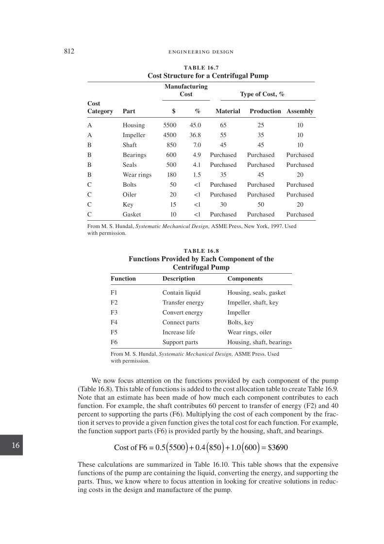
812 engineering design
16
TABLE 16.8
Functions Provided by Each Component of the Centrifugal Pump
Function Description Components
F1 Contain liquid Housing, seals, gasket
F2 Transfer energy Impeller, shaft, key
F3 Convert energy Impeller
F4 Connect parts Bolts, key
F5 Increase life Wear rings, oiler
F6 Support parts Housing, shaft, bearings
From M. S. Hundal, Systematic Mechanical Design, ASME Press. Used
with permission.
We now focus attention on the functions provided by each component of the pump (Table 16.8). This table of functions is added to the cost allocation table to create Table 16.9. Note that an estimate has been made of how much each component contributes to each function. For example, the shaft contributes 60 percent to transfer of energy (F2) and 40 percent to supporting the parts (F6). Multiplying the cost of each component by the frac-tion it serves to provide a given function gives the total cost for each function. For example, the function support parts (F6) is provided partly by the housing, shaft, and bearings.
Cost of F6 = 0.5 5500( ) + ( ) + ( ) =0 4 850 1 0 600 3. . $ 6690
These calculations are summarized in Table 16.10. This table shows that the expensive functions of the pump are containing the liquid, converting the energy, and supporting the parts. Thus, we know where to focus attention in looking for creative solutions in reduc-ing costs in the design and manufacture of the pump.
TABLE 16.7
Cost Structure for a Centrifugal Pump
Manufacturing Cost Type of Cost, %
Cost Category Part $ % Material Production Assembly
A Housing 5500 45.0 65 25 10
A Impeller 4500 36.8 55 35 10
B Shaft 850 7.0 45 45 10
B Bearings 600 4.9 Purchased Purchased Purchased
B Seals 500 4.1 Purchased Purchased Purchased
B Wear rings 180 1.5 35 45 20
C Bolts 50 <1 Purchased Purchased Purchased
C Oiler 20 <1 Purchased Purchased Purchased
C Key 15 <1 30 50 20
C Gasket 10 <1 Purchased Purchased Purchased
From M. S . Hundal , Systematic Mechanical Design, ASME Press, New York , 1997 . Used
with permission.
die37039_ch16.indd 812 2/25/08 7:03:14 PM

chapter 16: Cost Evaluat ion 813
16
TABLE 16.10
Calculation of Function Costs for Centrifugal Pump
Function Part
% of Part Cost for Function Part Cost, $
Function Cost of Individual
Part, $
Total Function Cost
$ %
F1: Contain Liquid
Housing 50 5500 2750
Seals 100 500 500
Gasket 100 10 10 3260 26.7
F2: Transfer Energy
Impeller 30 4500 1350
Shaft 60 850 510
Key 80 15 12 1872 15.3
F3: Convert Energy
Impeller 70 4500 3150 3150 25.8
F4: Connect Parts
Key 20 15 3
Bolts 100 50 50 53 0.4
F5: Increase Life
Wear rings 100 180 180
Oiler 100 20 20 200 1.6
F6: Support Parts
Housing 50 5500 2750
Shaft 40 850 340
Bearings 100 600 600 3690 30.2
From M. S . Hundal , Systematic Mechanical Design, ASME Press. New York , 1997 . Used with permission.
TABLE 16.9
Cost Structure for Centrifugal Pump with Function Cost Allocation
Manufacturing Cost Type of Cost, %
Cost Class Part $ % Material Production Assembly
Function Allocation, %
A Housing 5500 45.0 65 25 10 F1 50 F6 50
A Impeller 4500 36.8 55 35 10 F2 30 F3 70
B Shaft 850 7.0 45 45 10 F2 60 F6 40
B Bearings 600 4.9 Purchased Purchased Purchased F6 100
B Seals 500 4.1 Purchased Purchased Purchased F1 100
B Wear rings 180 1.5 35 45 20 F5 100
C Bolts 50 ,1 Purchased Purchased Purchased F4 100
C Oiler 20 ,1 Purchased Purchased Purchased F5 100
C Key 15 ,1 30 50 20 F2 80 F4 20
C Gasket 10 ,1 Purchased Purchased Purchased F1 100
From M. S . Hundal , Systematic Mechanical Design, ASME Press, New York , 1997 . Used with permission.
die37039_ch16.indd 813 2/25/08 7:03:15 PM

814 engineering design
16
A
One work cycleN
um
be
r o
f p
iece
s
1
LW = load workpiece
AT = advance the tool
RT = retract the tool
UW = unload workpiece
2
0
2A
CostUWRTCutATLWUWRTCutATLW
FIGURE 16.6 Elements of a machining operation.
16.12 MANUFACTURING COST MODELS
The importance of modeling in the design process was illustrated in Chap. 10. Mod-eling can show which elements of a design contribute most to the cost; that is, it can identify cost drivers. With a cost model it is possible to determine the conditions that minimize cost or maximize production (cost optimization). We have already seen that cost models aid signiB cantly in the selection of which process to use to make a part.
16.12.1 Machining Cost Model
Extensive work has been done on cost models for metal removal processes. 32 Bro-ken down into its simplest cost elements, a machining process can be described by Fig. 16.6. The time designated A is the machining plus work-handling costs per piece. If B is the tool cost, including the costs of tool changing and tool grinding, in dollars per tool, then
Cost/piece =nA B
nA
B
n
+= + (16.28)
where n is the number of pieces produced per tool.
32. E. J. A . Armarego and R. H . Brown , The Machining of Metals, Chap. 9, Prentice Hall, Englewood Cliffs, NJ , 1969 ; G . Boothroyd and W. A . Knight , Fundamentals of Machining and Machine Tools, 3d ed., CRC Press, Beca Raton, FL , 2006 .
die37039_ch16.indd 814 2/25/08 7:03:16 PM

chapter 16: Cost Evaluat ion 815
16
We shall now consider a more detailed cost model for turning down a bar on a lathe (Fig. 16.7). The machining time for one cut, t c , is
tL
V
L
fN
L
f
D
vc
feed
= = =12
(16.29)
where Vfeed 5 feed velocity, in. /minf 5 feed rate, in. /rev
N 5 rotational velocity, rev/minD 5 work diameter, in.v 5 cutting velocity, ft/mm
Equation (16.29) holds in detail only for the process of turning a cylindrical bar. For other geometries or other processes such as milling or drilling, different expressions would be used for L or V feed .
The total cost of a machined part is the sum of the machining cost C mc , the cost of the cutting tools, C t , and the cost of the material C m .
C C C Cu mc t m
= + + (16.30)
where C u is the total unit (per piece) cost. The machining cost, C mc ($/h), depends on the machining time t unit and the costs of the machine, labor, and overhead.
C M OH W OH tmc m op unit
= +( ) + +( )
1 1 (16.31)
where M is maching cost rate, $/hOHm is machine overhead rate, decimalW is labor rate for machine operator, $/hOHop is operator overhead rate, decimal
L
ND
FeedTool
Depth
of cut
FIGURE 16.7 Details of lathe turning.
die37039_ch16.indd 815 2/25/08 7:03:16 PM

816 engineering design
16
The machine cost includes the cost of interest, depreciation, and maintenance. It is found with the methods of Chap. 18 by determining these costs on an annual basis and converting them to per-hour costs on the basis of the number of hours the machine is used in the year. The machine overhead cost includes the cost of power and other services and a proportional share of the building, taxes, insurance, and other such expenses.
The production time for a unit is the sum of the machining time t m and the non-production or idle time t i .
t t tunit m i
= + (16.32)
The machining time t m is the machining time for one cut, t c , multiplied by the number of cuts.
t tm c
= ( )number of cuts (16.33)
The idle time is given by
t t t t ti set change hand down
= + + + (16.34)
where tset 5 total time fo job setup divided by number of parts in the batchtchange 5 prorated time for changing the cutting tool
= tool change timetool life
×t
m
thand 5 time the maching operator spends loading and unloading the work on the machine
tdown 5 downtime lost because of machine or tool failure, waiting for mate-rial or tools, or maintenance operations, Downtime is prorated per units production.
An important cost component is the cost of cutting tools. Tools lose their cut-ting edge from the extreme wear and high temperature generated at the tool-metal interface. The cost of tooling is the cost of cutting tools and a prorated cost of special B xtures used to hold the tool bits. The cost of the cutting tool per unit piece is
C Ct
Tt tool
m= (16.35)
where Ctool is the cost of a cutting tool, $tm is the machining time (min), given by Eq. (16.33)T is the tool life (min) given by Eq. (16.36)
Tool life usually is expressed by the Taylor tool life equation, which relates tool life T to surface velocity v .
vT Kp = (16.36)
die37039_ch16.indd 816 2/25/08 7:03:16 PM
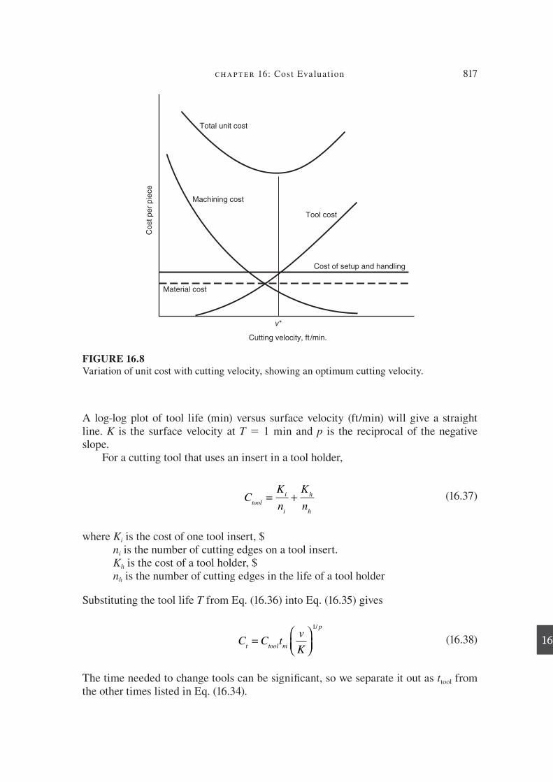
chapter 16: Cost Evaluat ion 817
16
A log-log plot of tool life (min) versus surface velocity (ft/min) will give a straight line. K is the surface velocity at T 5 1 min and p is the reciprocal of the negative slope.
For a cutting tool that uses an insert in a tool holder,
CK
n
K
ntool
i
i
h
h
= + (16.37)
where Ki is the cost of one tool insert, $ni is the number of cutting edges on a tool insert.Kh is the cost of a tool holder, $nh is the number of cutting edges in the life of a tool holder
Substituting the tool life T from Eq. (16.36) into Eq. (16.35) gives
C C tv
Kt tool m
p
=
1/
(16.38)
The time needed to change tools can be signiB cant, so we separate it out as t tool from the other times listed in Eq. (16.34).
Cutting velocity, ft /min.
Machining cost
Total unit cost
Tool cost
Cost of setup and handling
Material cost
v*
Co
st
pe
r p
iece
FIGURE 16.8 Variation of unit cost with cutting velocity, showing an optimum cutting velocity.
die37039_ch16.indd 817 2/25/08 7:03:17 PM
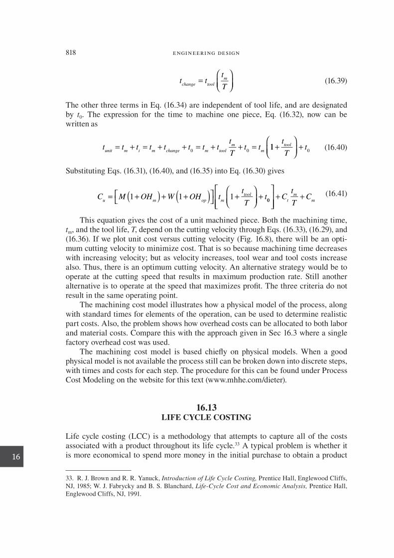
818 engineering design
16
t tt
Tchange tool
m=
(16.39)
The other three terms in Eq. (16.34) are independent of tool life, and are designated by t 0 . The expression for the time to machine one piece, Eq. (16.32), now can be written as
t t t t t t t tt
Tt t
unit m i m change m tool
m
m= + = + + = + + =
0 011
0+
+
t
Tttool (16.40)
Substituting Eqs. (16.31), (16.40), and (16.35) into Eq. (16.30) gives
C M OH W OH tt
Tt
u m op m
tool= +( ) + +( )
+
+1 1 1
00
+ +Ct
TC
t
m
m
(16.41)
This equation gives the cost of a unit machined piece. Both the machining time, t m , and the tool life, T , depend on the cutting velocity through Eqs. (16.33), (16.29), and (16.36). If we plot unit cost versus cutting velocity (Fig. 16.8), there will be an opti-mum cutting velocity to minimize cost. That is so because machining time decreases with increasing velocity; but as velocity increases, tool wear and tool costs increase also. Thus, there is an optimum cutting velocity. An alternative strategy would be to operate at the cutting speed that results in maximum production rate. Still another alternative is to operate at the speed that maximizes proB t. The three criteria do not result in the same operating point.
The machining cost model illustrates how a physical model of the process, along with standard times for elements of the operation, can be used to determine realistic part costs. Also, the problem shows how overhead costs can be allocated to both labor and material costs. Compare this with the approach given in Sec 16.3 where a single factory overhead cost was used.
The machining cost model is based chieD y on physical models. When a good physical model is not available the process still can be broken down into discrete steps, with times and costs for each step. The procedure for this can be found under Process Cost Modeling on the website for this text (www.mhhe.com/dieter).
16.13 LIFE CYCLE COSTING
Life cycle costing (LCC) is a methodology that attempts to capture all of the costs associated with a product throughout its life cycle. 33 A typical problem is whether it is more economical to spend more money in the initial purchase to obtain a product
33. R. J . Brown and R. R . Yanuck , Introduction of Life Cycle Costing, Prentice Hall, Englewood Cliffs, NJ , 1985 ; W. J . Fabrycky and B. S . Blanchard , Life-Cycle Cost and Economic Analysis, Prentice Hall, Englewood Cliffs, NJ , 1991 .
die37039_ch16.indd 818 2/25/08 7:03:17 PM

chapter 16: Cost Evaluat ion 819
16
with lower operating and maintenance costs, or whether it is less costly to purchase a product with lower B rst costs but higher operating costs. Life cycle costing goes into the analysis in much detail in an attempt to evaluate all relevant costs, both present and future.
The costs that enter into life cycle costing can be divided into B ve categories.
First costs . Purchase cost of equipment or plant. One - time costs . Cost for transportation, installation, training of operating personnel, startup, and hazardous material cleanup and disposal of equipment upon retirement.
Operating costs . Wages for production or operating personnel, utilities, supplies, materials, disposal of hazardous materials.
Maintenance costs . Cost for service, inspection, and repair or replacement of equipment.
Other costs . Taxes and insurance.
Life cycle costing, also known as “whole life costing,” B rst found strong advocates in the area of military procurement, where it is used to compare competing weapons systems. 34 A typical piece of military hardware, with a service life of 20 years, can have operation and maintenance costs 60 to 80 percent of the life cycle cost.
Life cycle costing has been combined with life cycle assessment (see Sec. 8.9) of the costs of energy consumption and pollution during manufacture and service, and the costs of retiring the product when it reaches its useful life. Expansion of the cost models beyond the traditional bounds to include pollution and disposal is an active area of research that will place the design engineer in a better position to make critical trade-off decisions.
Typical elements in the life cycle of a product are shown in Fig. 16.9. This B gure emphasizes the overlooked impact on society costs (OISC) that are rarely quantiB ed and incorporated into a product life cycle analysis. 35 Starting with design, the actual costs incurred here are a small part of the LCC, but the costs committed in design comprise about 75 percent of the avoidable costs within the life cycle of the product. Moreover, it is about 10 times less costly to make a change or correct an error in design than in manufacturing. Acquiring the raw materials, usually by mining or oil extrac-tion, and processing the materials, can create large environmental costs. These areas also often have considerable inventory and transportation costs. We have concentrated in previous sections on the costs in manufacturing and assembly of products.
The cost of ownership of a product is the traditional aspect of LCC. Useful life is commonly measured by cycles of operation, length of operation, or shelf life. In de-sign we attempt to extend life for use and service by using durable and reliable materi-als and components. Product obsolescence is dealt with through modular products.
Maintenance costs, especially maintenance labor costs, usually dominate other use/service costs. Most analyses divide maintenance costs into scheduled or preven-tive maintenance and unscheduled or corrective maintenance. The mean time between failure and the mean time to repair are important parameters from reliability theory
●
●
●
●
●
34 . MIL-HDBK 259, Life Cycle Costs in Navy Acquisitions. 35. N . Nasr and E. A . Varel , “ Total Product Life-Cycle Analysis and Costing ,” Proceedings of the 1997
Total Life Cycle Conference, P-310, pp. 9–15 , Society of Automotive Engineers, Warrendale, PA , 1997 .
die37039_ch16.indd 819 2/25/08 7:03:17 PM
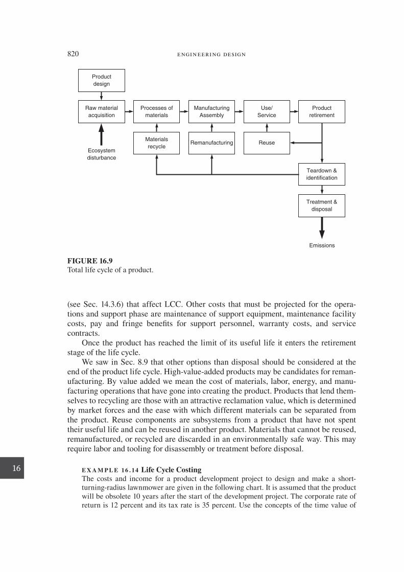
820 engineering design
16
(see Sec. 14.3.6) that affect LCC. Other costs that must be projected for the opera-tions and support phase are maintenance of support equipment, maintenance facility costs, pay and fringe beneB ts for support personnel, warranty costs, and service contracts.
Once the product has reached the limit of its useful life it enters the retirement stage of the life cycle.
We saw in Sec. 8.9 that other options than disposal should be considered at the end of the product life cycle. High-value-added products may be candidates for reman-ufacturing. By value added we mean the cost of materials, labor, energy, and manu-facturing operations that have gone into creating the product. Products that lend them-selves to recycling are those with an attractive reclamation value, which is determined by market forces and the ease with which different materials can be separated from the product. Reuse components are subsystems from a product that have not spent their useful life and can be reused in another product. Materials that cannot be reused, remanufactured, or recycled are discarded in an environmentally safe way. This may require labor and tooling for disassembly or treatment before disposal.
E X A M P L E 1 6 . 14 Life Cycle Costing The costs and income for a product development project to design and make a short- turning-radius lawnmower are given in the following chart. It is assumed that the product will be obsolete 10 years after the start of the development project. The corporate rate of return is 12 percent and its tax rate is 35 percent. Use the concepts of the time value of
Product
design
Raw material
acquisition
Ecosystem
disturbance
Processes of
materials
Manufacturing
Assembly
Use/
Service
Product
retirement
Materials
recycleRemanufacturing Reuse
Teardown &
identification
Treatment &
disposal
Emissions
FIGURE 16.9 Total life cycle of a product .
die37039_ch16.indd 820 2/25/08 7:03:17 PM

chapter 16: Cost Evaluat ion 821
16
* The concepts of engineering economy, based on time value of money are considered in Chap. 18 found at the text website, www. mhhe.com/dieter.
money* to B nd the net present value (NPV) of the project and the average annual proB t margin based on sales.
CategoryYr1
Yr2
Yr3
Yr4
Yr5
Yr6
Yr7
Yr8
Yr9
Yr10 Avg.
1. Development costs 0.8 1.90 0.4 0.4 0.4 0.4 0.4 0.2 0.2 0.2
2. Cost of product sold 12.0 13.5 15.0 16.1 16.8 16.0 15.2 15.3 14.8
3. Sales & marketing 2.1 3.0 3.5 2.8 2.7 2.8 2.9 2.6 2.8
4. G&A plus overhead 0.8 1.5 2.0 2.0 2.0 2.0 2.0 2.0 1.7
5. Special production equipment, P
4.1
6. Salvage value, S 0.5
7. Depreciation on equip. 0.4 0.4 0.4 0.4 0.4 0.4 0.4 0.4 0.4 0.4
8. Environ. cleanup 1.1
9. Net sales 28.2 31.3 36.2 39.8 40.0 39.1 38.0 35.0 35.95
All gures in millions of dollars .
Present Value of Costs
(1) PV of development costs 5 0.8( P / F ,12,1) 1 1.90 ( P / F ,12,2) 1 0.4( P / A ,12,5)( P / F ,12,2) 1 0.2( P / A ,12,3)( P / F ,12,7) 5 $3.47M
(2) PV of cost of product sold 5 14.8( P / A ,12,8)( P / F ,12,2) 5 $58.7M (3) PV of sales and marketing costs 5 2.8( P / A ,12,8)( P / F ,12,2) 5 $11.17M (4) PV of G&A and overhead 5 1.7( P / A ,12,8)( P / F ,12,2) 5 $6.73M (5) Annual straight-line depreciation charge on (5), year 2 through 10 5 ( P 2 S )/ n 5
(4.1 2 0.5)/9 5 0.40. (7) PV of depreciation 5 0.4( P / A ,12,9)( P / F ,12,1) 5 $1.90M (8) PV of cost of environmental cleanup 5 1.1( P / F ,12,10) 5 $0.35M
Present value of total costs = 3.47 + 58.70 + 11.17 + 6.73 + 1.90 + 0.35 = $82.32
Present Value of Income or Savings
(9) Present value of net sales 5 35.95( P / A ,12,8)( P / F ,12,2) 5 $130.8M Present value of sale of equipment for salvage PV 5 0.5( P / F ,12,10) 5
$0.16M Present value of tax reduction (0.35)(1.90) 5 $0.66M Present value of total income or savings 5 $131.6M
die37039_ch16.indd 821 2/25/08 7:03:18 PM

822 engineering design
16
Net present value 5 present value of income 2 present value of costs 5 131.6 2 82.3 5 $ 49.3M over 10 years, or an average of $ 4.93M per year
Annual proB t margin 5 4.93/35.95 5 13.7% per year
Note that an average of annual income and cost was used to simplify calculation. The use of a spreadsheet would have given more accurate numbers, but this is not warranted by the precision of the estimates.
16.14 SUMMARY
Cost is a primary factor of design that no engineer can afford to ignore. It is important to understand the basics of cost evaluation so that you can produce high-functioning, low-cost designs. Cost buildup begins in conceptual design and continues through em-bodiment and detail design.
To be cost literate you need to understand the meaning of such concepts as non-recurring costs, recurring costs, B xed costs, variable costs, direct costs, indirect costs, overhead, and activity-based costing.
Cost estimates are developed by three general methods.
Cost estimation by analogy with previous products or projects. This method re-quires past experience or published cost data. Because this uses historical data, the estimates must be corrected for price inD ation using cost indexes, and for dif-ferences of scale using cost-capacity indexes. This method is often used in the conceptual phase of design. The parametric or factor approach uses regression analysis to correlate past costs with critical design parameters like weight, power, and speed, Software programs that use parametric relationships and cost databases are becoming increasingly useful for the calculation of costs in conceptual and embodiment design. A detailed breakdown of all the steps required to manufacture a part with an as-sociated cost of materials, labor, and overhead for each step for each operation is needed to determine the cost to produce the part. This method is generally used in the B nal cost estimates in the detail design stage.
Costs may sometimes be related to the functions performed by the design. This is a situation highly to be desired, because it allows optimization of the design concept with respect to cost.
Manufacturing costs generally decrease with time as more experience is gained in making a product. This is known as a learning curve.
Computer cost models are gaining in use as a way to pinpoint the steps in a manu-facturing process where cost savings must be achieved. Simple spreadsheet models are useful for determining product proB tability and making trade-offs between as-pects of the business situation.
Life cycle costing attempts to capture all the costs associated with a product throughout its life cycle, from design to retirement from service. Originally LCC fo-cused only on the costs incurred in using a product, such as maintenance and repair,
1.
2.
3.
die37039_ch16.indd 822 2/25/08 7:03:18 PM
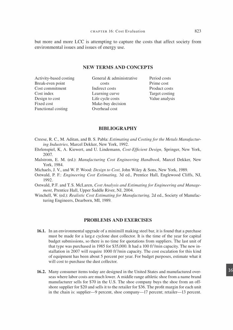
chapter 16: Cost Evaluat ion 823
16
BIBLIOGRAPHY
Creese , R. C ., M . Aditan , and B. S . Pabla : Estimating and Costing for the Metals Manufactur-
ing Industries, Marcel Dekker, New York , 1992 . Ehrlenspiel , K , A . Kiewert , and U . Lindemann , Cost-Ef! cient Design, Springer, New York ,
2007 . Malstrom , E. M . (ed.): Manufacturing Cost Engineering Handbook, Marcel Dekker, New
York , 1984 . Michaels , J. V ., and W. P . Wood : Design to Cost, John Wiley & Sons, New York , 1989 . Ostwald , P. F .: Engineering Cost Estimating, 3d ed., Prentice Hall, Englewood Cliffs, NJ ,
1992 . Ostwald , P. F . and T. S . McLaren , Cost Analysis and Estimating for Engineering and Manage-
ment, Prentice Hall, Upper Saddle River, NJ , 2004 . Winchell , W . (ed.): Realistic Cost Estimating for Manufacturing, 2d ed., Society of Manufac-
turing Engineers, Dearborn, MI , 1989 .
PROBLEMS AND EXERCISES
16.1. In an environmental upgrade of a minimill making steel bar, it is found that a purchase must be made for a larg.e cyclone dust collector. It is the time of the year for capital budget submissions, so there is no time for quotations from suppliers. The last unit of that type was purchased in 1985 for $35,000. It had a 100 ft 3 /min capacity. The new in-stallation in 2007 will require 1000 ft 3 /min capacity. The cost escalation for this kind of equipment has been about 5 percent per year. For budget purposes, estimate what it will cost to purchase the dust collector.
16.2. Many consumer items today are designed in the United States and manufactured over-seas where labor costs are much lower. A middle range athletic shoe from a name brand manufacturer sells for $70 in the U.S. The shoe company buys the shoe from an off-shore supplier for $20 and sells it to the retailer for $36. The proB t margin for each unit in the chain is: supplier—9 percent, shoe company—17 percent; retailer—13 percent.
but more and more LCC is attempting to capture the costs that affect society from environmental issues and issues of energy use.
Activity-based costing Break-even point Cost commitment Cost index Design to cost Fixed cost Functional costing
General & administrative costs
Indirect costs Learning curve Life cycle costs Make-buy decisionOverhead cost
Period costs Prime cost Product costs Target costing Value analysis
NEW TERMS AND CONCEPTS
die37039_ch16.indd 823 2/25/08 7:03:19 PM

824 engineering design
16
Estimate the major categories of cost breakdown for each unit in the chain. Do this as a team problem and compare the results for the entire class.
16.3. The type of tooling to make for a manufacturing process depends on the expected to-tal quantity of parts. Tooling made from standard components and less wear-resistant materials (soft tooling) can be made more quickly and cheaply than conventional tool-ing made from hardened steel (hard tooling). Use the concept of break-even point to determine the production quantity for which soft tooling can be justiB ed. The follow-ing cost data applies:
Soft Tooling Hard Tooling
Tooling cost C S $600 C H $7500
Setup cost S S $100 S H $60
Unit part cost C ps $3.40 C pH $0.80
The total production run is expected to be 5000 units. Parts are made in batches of 500.
16.4. A manufacturer of small hydraulic turbines has the annual cost data given here. Calcu-late the manufacturing cost and the selling price for a turbine.
Raw material and components costs $2,150,000
Director labor 950,000
Direct expenses 60,000
Plant manager and staff 180,000
Utilities for plant 70,000
Taxes and insurance 50,000
Plant and equipment depreciation 120,000
Warehouse expenses 60,000
OfB ce utilities 10,000
Engineering salaries (plant) 90,000
Engineering expenses (plant) 30,000
Administrative staff salaries 120,000
Sales staff, salaries and commissions 100,000
Total annual sales: 60 units
ProB t margin: 15%
16.5. A jewel case for a compact disc is made from polycarbonate ($2.20 per lb) by a ther-moplastic molding process. Each CD case uses 20 grams of plastic. The parts will be made in a 10-cavity mold that makes 1400 parts per hour at an operating cost of $20 per hour. Manufacturing overhead is 40 percent. Since the parts are sold in large lots, the G&A expenses are a low 15 percent. ProB t is 10 percent. What is the estimated selling price of each CD case?
16.6. Two competing processes for making high-quality vacuum melted steel are the vac-uum arc reB ning process (VAR) and electroslag remelting (ESR). The estimated costs for operating each of the processes are:
die37039_ch16.indd 824 2/25/08 7:03:19 PM

chapter 16: Cost Evaluat ion 825
16
Cost Component VAR ESR
Direct labor, one melter and one helper
$89,000 $89,000
Manufacturing overhead, 140% direct labor
$124,600 $124,600
Melting power 0.3 kWh/lb 1000 lb/h 10¢/kWh
0.5 kWh/lb 1250 lb/h 10¢/kWh
Cooling water (annual charge)
$5,500 $6,800
Slag — $42,000
The capital cost of a VAR system is $1.3M and for an ESR system it is $0.9M. Each melting system has a 10-year useful life. Each uses 1000 ft 2 of factory space, which costs $40 per ft 2 . Assume both furnaces operate for 15 eight-hour shifts per week for 50 weeks in the year. Estimate the cost of melting a pound of high-grade steel for each process.
16.7. The accounting department established the costs given in the following table for pro-ducing two products, X and Z, over a given time period.
(a) Give an example of typical costs that would be put in each of the 10 cost catego-ries listed.
(b) Determine the overhead and unit cost for each product in terms of direct labor cost.
(c) Determine the overhead and unit cost for each product on the basis of direct labor hours (DLH).
(d) Determine the overall overhead rate per DLH and use it to determine the unit cost of product X.
(e) Determine the overhead and unit cost for each product on the basis of the propor-tion of direct material costs.
Item Product X Product Z
Quantity 3000 5000
Machine hours 70 90
Direct labor hours (DLH) 400 600
Factory D oor space 150 50
Labor Rate $/h
Labor Amount, h
Material Cost $/unit
Material Amount, units Cost $
Product X
Direct labor 18.00 400 7,200
Direct material 6.50 3000 19,500
Product Z
Direct labor 14.00 600 8,400
Direct material 7.50 5000 37,500
die37039_ch16.indd 825 2/25/08 7:03:19 PM
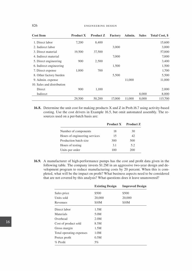
826 engineering design
16
Cost Item Product X Product Z Factory Admin. Sales Total Cost, $
1. Direct labor 7,200 8,400 15,600
2. Indirect labor 3,000 3,000
3. Direct material 19,500 37,500 57,000
4. Indirect material 7,000 7,000
5. Direct engineering 900 2,500 3,400
6. Indirect engineering 1,500 1,500
7. Direct expense 1,000 700 1,700
8. Other factory burden 5,500 5,500
9. Admin. expense 11,000 11,000
10. Sales and distribution
Direct 900 1,100 2,000
Indirect 8,000 8,000
29,500 50,200 17,000 11,000 8,000 115,700
16.8. Determine the unit cost for making products X and Z in Prob.16.7 using activity-based costing. Use the cost drivers in Example 16.5, but omit automated assembly. The re-sources used on a per-batch basis are:
Product X Product Z
Number of components 18 30
Hours of engineering services 15 42
Production batch size 300 500
Hours of testing 3.1 5.2
Units per order 100 200
16.9. A manufacturer of high-performance pumps has the cost and proB t data given in the following table. The company invests $1.2M in an aggressive two-year design and de-velopment program to reduce manufacturing costs by 20 percent. When this is com-pleted, what will be the impact on proB t? What business aspects need to be considered that are not covered by this analysis? What questions does it leave unanswered?
Existing Design Improved Design
Sales price $500 $500
Units sold 20,000 20,000
Revenues $10M $10M
Direct labor 1.5M
Materials 5.0M
Overhead 2.0M
Cost of product sold 8.5M
Gross margin 1.5M
Total operating expenses 1.0M
Pretax proB t 0.5M
% ProB t 5%
die37039_ch16.indd 826 2/25/08 7:03:20 PM

chapter 16: Cost Evaluat ion 827
16
16.10. A company has received an order for four sophisticated space widgets. The buyer will take delivery of one unit at the end of the B rst year and one unit at the end of each of the succeeding three years. He will pay for a unit immediately upon receipt and not before. However, the manufacturer can make the units ahead of time and store them at negligible cost for future delivery.
The chief component of cost of the space widget is labor at $25 per h. All units made in the same year can take advantage of an 80 percent learning curve. The B rst unit requires 100,000 h of labor. Learning occurs only in one year and is not carried over from year to year. If money is worth 16 percent after a 52 percent tax rate, decide whether it would be more economical to build four units the B rst year and store them, or build one unit in each of the four years.
16.11. Develop a cost model to compare the cost of drilling 1000 holes in steel plate with a standard high-speed steel drill and a TiN-coated H.S.S. drill. Each hole is 1 in. deep. The drill feed is 0.010 per rev. Machining time costs $10 per minute, and the cost of changing a tool is $5.
Tool Life (No. of Holes)
Price of a Drill 500 rpm 900 rpm
Std. H.S.S. drill $12.00 750 80
TiN-coated H.S.S. $36.00 1700 750
(a) Compare the costs at B xed conditions of 500 rpm. (b) Compare the costs at a constant tool life of 750 holes.
16.12. Determine which system is more economical on a life cycle costing basis.
System A System B
Initial cost $300,000 $240,000
Installation 23,000 20,000
Useful life 12 years 12 years
Operators needed 1 2
Operating hours 2100 2100
Operating wage rate $20 per h $20 per h
Parts and supplies cost (% of initial cost) 1% 2%
Power 8 kW at 10¢/kWh 9 kW at 10¢/kWh
Escalation of operating costs 6% 6%
Mean time between failures 600 h 450 h
Mean time to repair 35 h 45 h
Maintenance wage rate $23 per h $23 per h
Maintenance escalation rate 6% 6%
Desired rate of return 10% 10%
Tax rate 45% 45%
16.13. Discuss the automobile safety standards and air pollution standards in terms of the concept of life cycle costs.
die37039_ch16.indd 827 2/25/08 7:03:20 PM

828
17
LEGAL AND ETHICAL ISSUES IN
ENGINEERING DESIGN
17.1 INTRODUCTION
Engineering is not only applying scienti0 c laws and principles to technical problems. It is focused on improving the lot of society, and as such, it brings engineers into the mainstream of business and industry. Almost all entry-level engineers become in-volved, at least tangentially, with situations that call for some understanding of the law and situations that call for ethical judgments. Therefore, this chapter presents a brief overview of some legal and ethical issues in engineering. With topics as broad as law and ethics we can only scratch the surface, so we have chosen to focus on those issues that are most pertinent to engineering design.
The following are examples of where a design engineer might be concerned with legal and ethical issues:
Preparing a contract to secure the services of a product data management 0 rm. Reviewing a contract to determine whether a contractor who built an automated production facility has satisfactorily full0 lled the terms of a contract.
Deciding whether it is legal and ethical to reverse engineer a product. Managing a design project to avoid the possibility of a product liability suit. Protecting the intellectual property created as part of a new product development activity.
Deciding whether to take a job with a direct competitor that is bidding on a contract in the area where you are now working.
The law is a formalized code of conduct describing what society feels is the proper way to behave. In other words, laws reH ect what society values. As society evolves, its attitude toward behavior changes, and the laws change as well. Also, the evolution of technology creates new ethical issues. Ethics is the study of human conduct that lays out the moral ground rules. It is intimately related to the values of society. Thus, laws and ethics, while distinct, are not independent. Ethical conduct is the behavior desired
●
●
●
●
●
●
die37039_ch17.indd 828 2/25/08 7:21:00 PM

chapter 17: Legal And Ethical Issues In Engineer ing Design 829
by society that is separate from the minimum standards of the law. For example, mak-ing a defective product despite taking all due care may subject you to product liability law, but it is not generally considered unethical.
This chapter comes with a warning label. A little knowledge can be a dangerous
thing. Just as we would not expect a lawyer to practice engineering, so an engineer should not practice law. One objective of this chapter is to give you enough knowl-edge about the legal aspects of engineering practice to recognize when you need to take certain actions or to know when to seek legal counsel. A second objective is to help you realize that the engineering profession has expectations for your conduct and that a true professional recognizes responsibilities to the employer, the profession, and society, not just those to himself or herself.
17.2 THE ORIGIN OF LAWS
The code of American law has its origin in English common law. These laws derived from agreed-upon tradition and custom and were given the authority of law by deci-sions in the courts. Since each court decision is based on the study of previous court cases, it is often called case law.
Statutory law is law that is created by a legislative body, either state or federal. These laws, known as statutes, are often codi0 ed, as opposed to common law, and prescribe particular actions that apply to speci0 c situations. Statutes may modify, re-verse, or abolish common law doctrines. They are subject to both change and extinc-tion by legislative action.
While the two basic types of law are common law and statutory law, many po-litical entities contribute to the body of law. Constitutional law, which is based on the Constitution of the United States, de0 nes governmental powers, especially with respect to the states, and secures the rights of the individual citizen. Municipal law is a subdivision of statutory law that is produced by towns and cities. Municipal
ordinances deal with issues like traf0 c laws, zoning, and building codes. A large body of administrative law has been created by rulings and regulations of federal and state agencies other than the courts. Examples are OSHA and the EPA. Although cases in-volving administrative law are usually handled within the agency, disputes are 0 nally resolved through the regular court system.
The legal system is divided into criminal law and civil law. Most of us who watch television are familiar with criminal law, but the majority of cases are concerned with civil law. There are several important distinctions between the two forms of le-gal practice. In criminal law, emphasis is placed on whether the defendant is inno-cent or guilty. The defendant is assumed innocent until proven guilty. The defendant must be found guilty beyond a reasonable doubt by a unanimous verdict of a jury of his peers. The penalty for being found guilty is imprisonment or in extreme cases, death.
The issue of guilt or innocent is not at question in a civil case. Here the question is which of the parties failed to live up to an agreement or acted improperly in a way that caused someone damage. In a civil trial the jury is not required to be unanimous in its
die37039_ch17.indd 829 2/25/08 7:21:01 PM

830 engineering design
verdict, and it is only necessary to reach the verdict based on the preponderance of the evidence, as opposed to the higher standard in a criminal case. The winner in a civil case is usually awarded monetary damages or custody of the disputed property.
The purpose of the legal system is to protect and make life easier for each member of society. The rule of law is important not only in criminal matters, but it affects other aspects of society like politics and the economy.
17.3 CONTRACTS
A contract is a promise by one person to another to do or not to do something. Only promises that the law will enforce are contracts. The three elements of a contract are:
Contract 5 offer 1 acceptance 1 consideration
An offer is an expression made by one person that leads another person to reason-ably expect that the promisor wishes to create an agreement. The offer must be clear, de0 nite, and speci0 c, with no room for serious misunderstanding. An acceptance of the offer is necessary to make a contract legally binding. Both the offer and the acceptance must be voluntary acts. A contract cannot be forced on anyone. A contract is not enforceable by law unless it contains an agreement to exchange promises with value, the consideration. For example, if A and B enter into a contract in which A promises to pay B $1000 for modifying a CAD software package, both the money and the service are considerations.
17.3.1 Types of Contracts
Contracts can take many forms. They may be classi0 ed as express or implied, bilateral or unilateral. Also, a contract may be either written or verbal. Examples of contracts are purchase contracts, leases, a contract to perform a service, or an employment contract.
An express contract is a contract in which all of the terms are agreed upon and expressed in words, either written or oral. An oral contract, once made, can be just as legal as a written contract, but it is much more dif0 cult to prove and enforce. Moreover, many states have statutes of fraud that require writing for certain con-tracts to be enforceable.
An implied contract is a contract in which the agreement between parties is in-ferred by the legal system wholly or in part by their actions. For example, Jim goes to the local convenience store, where he has an account. He picks up a Sunday New York Times and holds it up so the clerk sees him take it and the clerk nods in return as he leaves the store with the paper. Jim has made an implied contract to pay for the newspaper.
●
●
die37039_ch17.indd 830 2/25/08 7:21:01 PM

chapter 17: Legal And Ethical Issues In Engineer ing Design 831
A bilateral contract is a contract in which two parties have both made a promise to each other. A promise is made in return for a promise. Each party is both a promi-sor and a promisee.
A unilateral contract is one in which the promisor does not receive a promise as con-sideration for her promise but instead agrees to pay if she receives an act or service. For example, Mrs. Jones says to Johnny Smith, “I promise to pay you $100 tomorrow if you will clean out my basement and garage today.” Johnny immediately goes to work. This constitutes acceptance of the offer and creates a unilateral contract.
If more than one promisor or promisee is involved, the contract can take different forms (Table 17.1). The chief implication is with respect to the liabilities incurred by the different parties.
An engineer will have to deal with contracts in a number of different situations. Contracts for the purchase or sale of property are common. On taking a job you may be asked to sign a contract stating that all technical ideas that you develop belong to the company, even those conceived while not on the job. These contracts are often negotiable at the time of employment and are something to consider when you are looking for employment. In technical dealings between companies, one of the parties may be asked to sign a con! dentiality agreement. This is a contract in which one of the parties agrees to not disclose, make use of, or copy a design or product that the other party is about to disclose.
17.3.2 General Form of a Contract
In general, every business contract should contain the following information:
Introduction to the agreement. Include title and date. Name and address of all parties. If one of the parties is a corporation, it should be so stated. Complete details of the agreement. State all promises to be performed. Include such details as speci0 cations and expected outcomes. Give details on promises of payments, including amounts, timing of payments, and interest.
●
●
1.2.
3.
TABLE 17.1
Types of Contracts when There Is More than One Promisor or Promisee
Type of Contract Number of Parties Liability
Joint Two or more persons promise the same performance as a single party
All promisors are liable for the complete ful0 llment of the contract
Several Separate promises made by more than one promisor
Each promisor is liable for his or her individual promise
Joint and several Two or more parties make a joint contract but also state that they are individually liable for completion of contract
All promisors face cumulative liability
die37039_ch17.indd 831 2/25/08 7:21:02 PM
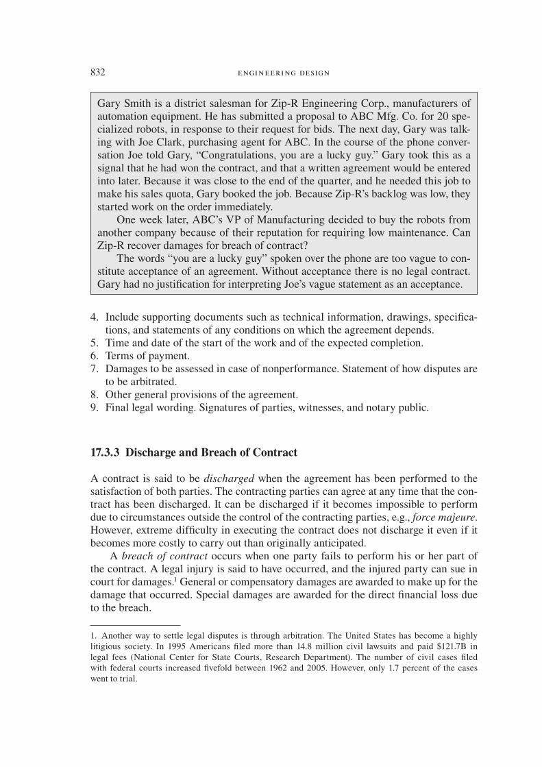
832 engineering design
Include supporting documents such as technical information, drawings, speci0 ca-tions, and statements of any conditions on which the agreement depends. Time and date of the start of the work and of the expected completion. Terms of payment. Damages to be assessed in case of nonperformance. Statement of how disputes are to be arbitrated. Other general provisions of the agreement. Final legal wording. Signatures of parties, witnesses, and notary public.
17.3.3 Discharge and Breach of Contract
A contract is said to be discharged when the agreement has been performed to the satisfaction of both parties. The contracting parties can agree at any time that the con-tract has been discharged. It can be discharged if it becomes impossible to perform due to circumstances outside the control of the contracting parties, e.g., force majeure . However, extreme dif0 culty in executing the contract does not discharge it even if it becomes more costly to carry out than originally anticipated.
A breach of contract occurs when one party fails to perform his or her part of the contract. A legal injury is said to have occurred, and the injured party can sue in court for damages. 1 General or compensatory damages are awarded to make up for the damage that occurred. Special damages are awarded for the direct 0 nancial loss due to the breach.
4.
5.6.7.
8.9.
1 . Another way to settle legal disputes is through arbitration. The United States has become a highly litigious society. In 1995 Americans 0 led more than 14.8 million civil lawsuits and paid $121.7B in legal fees (National Center for State Courts, Research Department). The number of civil cases 0 led with federal courts increased 0 vefold between 1962 and 2005. However, only 1.7 percent of the cases went to trial.
Gary Smith is a district salesman for Zip-R Engineering Corp., manufacturers of automation equipment. He has submitted a proposal to ABC Mfg. Co. for 20 spe-cialized robots, in response to their request for bids. The next day, Gary was talk-ing with Joe Clark, purchasing agent for ABC. In the course of the phone conver-sation Joe told Gary, “Congratulations, you are a lucky guy.” Gary took this as a signal that he had won the contract, and that a written agreement would be entered into later. Because it was close to the end of the quarter, and he needed this job to make his sales quota, Gary booked the job. Because Zip-R’s backlog was low, they started work on the order immediately.
One week later, ABC’s VP of Manufacturing decided to buy the robots from another company because of their reputation for requiring low maintenance. Can Zip-R recover damages for breach of contract?
The words “you are a lucky guy” spoken over the phone are too vague to con-stitute acceptance of an agreement. Without acceptance there is no legal contract. Gary had no justi0 cation for interpreting Joe’s vague statement as an acceptance.
die37039_ch17.indd 832 2/25/08 7:21:02 PM

chapter 17: Legal And Ethical Issues In Engineer ing Design 833
Often the terms of the contract contain liquidated damages that are agreed to beforehand in case the contract comes into dispute. If during trial these are found to be unreasonable, they will not come into force. The damages awarded at the trial will prevail. Note that the plaintiff has the obligation to act in such a way as to mini-mize the damages. If the court determines the damages could have been lessened through prudent action, this will be taken into consideration in setting the compensa-tory damages.
17.4 LIABILITY
Any party to a contract must be clear on the potential liability he or she is incurring. Liability means being bound or obligated to pay damages or restitution. Two ways
to incur liability are (1) breaking a contract or (2) committing a tort, such as fraud or negligence.
A breach of contract refers to violating a contract’s promise. Failure to deliver detail drawings of a new machine by the date speci0 ed in the contract is a breach of contract. It makes no difference whether this was done intentionally or not.
Fraud is intentional deceitful action aimed at depriving another party of his or her rights or causing injury in some respect. Examples would be double billing a client or falsely certifying that a component had passed the ASME pressure vessel code.
Negligence is failure to exercise proper care and provide expertise in accordance with the standards of the profession that results in damage to property or injury to per-sons. This is the most common way for an engineer to incur liability to the public. For example, an engineer fails to include a major source of loading in design calculations for a public project so that the design fails. Note that being honest and well- intentioned does not absolve the engineer from a legal charge of negligence.
To be liable for negligence it must be proved that the defendant did not take rea-sonable and prudent action. This is determined by a jury. One way to show reason-able care is to show that you acted at the current level of technological development, that is, the state of the art. A defense allowed in some states is to prove contributory
negligence, that the plaintiff was negligent or could have prevented the accident had due care been taken. Sometimes it can be shown that the plaintiff willingly took an unnecessary risk that he or she was aware of, as when a person dives into a pool where the depth is clearly marked at 3 ft.
The degree of risk concerning negligence depends on the way the business is or-ganized. In a sole proprietorship the owner and the business are one and the same. No distinction is made between the property of the business and that of the owner. Thus, if the business is sued for negligence, the owner is at risk of losing her own savings if the business does not have enough funds to pay the judgment of the court. A partner-
ship is close to a proprietorship but with many co-owners. All general partners are responsible for the acts and 0 nancial dealings of each other. A corporation is a legal entity that possesses many of the legal powers of individuals, but the corporation ex-ists independently of the people who own and manage it. A corporation can buy and
die37039_ch17.indd 833 2/25/08 7:21:02 PM

834 engineering design
sell property, enter into legal agreements, and sue and be sued. The personal 0 nances of the owners of a corporation are separate from those of the corporation.
The corporation will be held liable for the acts of an employee who commits a civil wrong while engaged in corporate business. For example, the corporation can be 0 ned by the EPA for the act of an employee who discharges liquid waste into a stream. Generally speaking, the corporation will incur the penalties of its employees, and the employee, in turn, may face the wrath of the corporation. Thus, working in a corpo-rate structure provides some degree of protection from liability, but it is not absolute protection. Employees of corporations have been sued in the courts for negligence. Moreover, the trend in the courts is toward greater accountability of corporate em-ployees. A corporate form cannot protect a professional from professional negligence.
17.5 TORT LAW
Contract law and tort law are the major divisions within civil law. A tort is a civil
wrong that involves damage committed against a person or his or her property, busi-ness, or reputation. It is a breach of the rights of an individual to be secure in his or her person and property and be free from undue harassment. 2 Tort law is chie> y case law of the state courts, rather than statutory law. A decision in a case based on tort law hinges on three questions:
Have a person’s rights been infringed upon? Did the act occur as a result of negligence or actual intent on the part of the defendant?
Did the plaintiff suffer damages as a result of the act?
Tort law deals with civil cases for which the penalty usually is monetary compen-sation rather than conE nement. The difference between a tort and a crime is that a tort is a civil wrong while a crime is a wrong against society that threatens the peace and safety of the community. The victim of a crime may also bring a tort suit against the defendant to recover damages.
Tort suits involving engineers usually are concerned with one of four types of actions: (1) misrepresentation, (2) nuisance, (3) negligence, and (4) product liability. Misrepresentation is a false statement by a person of a fact that is known to be false, with the intent to deceive another person. When done under oath, it is called perjury. Misrepresentation is often claimed in a breach of contract suit. Nuisance concerns the annoyance or disturbance of a person such that the use of property becomes physi-cally uncomfortable. Nuisances that affect the community, such as a blaring boom box at an open window, become a public nuisance. Negligence was deE ned in Sec. 17.4. Product liability is the action whereby an injured party seeks to recover dam-ages for injury to person or property from a manufacturer or seller when the plaintiff
●
●
●
2. Engineering Law, Design Liability, and Professional Ethics, Professional Publications, Belmont, CA , 1983 .
die37039_ch17.indd 834 2/25/08 7:21:02 PM

chapter 17: Legal And Ethical Issues In Engineer ing Design 835
alleges that a defective product or design caused the injury. This rapidly growing type of tort suit is discussed in Sec. 17.6.
17.6 PRODUCT LIABILITY
Product liability refers to the legal actions by which an injured party seeks to recover damages for personal injury or property loss from the producer or seller of a product. Product liability suits are pursued under the laws of tort. In no area of U.S. law has ac-tivity increased as dramatically as in personal injury product-liability civil law suits. These span the gamut from individual suits by a single plaintiff against a single com-pany to industrywide class action suits with tens of thousands of plaintiffs against all asbestos manufacturers. The costs associated with tort-based litigation, of which prod-uct liability and medical malpractice cases are the predominate share, are estimated to be over $300 billion per year. 3 This is based on annual damage awards and plaintiff and defense legal fees. The authors estimate the real costs of tort-based cases to be at least twice this amount as companies shift product development funding to R&D aimed at defending product liability cases. In extreme cases it has resulted in the near demise of once-proE table industries. In the 1970s the annual production of piston-engine powered light planes was from 10,000 to 15,000 per year and accounted for more than 100,000 jobs. In the early 1990s production was barely 500 planes per year. This decrease has been attributed to the high cost of product liability litigation in the industry. 4
Bill Garrison was hired by ABC Mfg. Co. as a consultant in plastic processing, with a chemical engineering degree and 10 years of experience. He was asked to recom-mend the equipment needed to convert a certain product line from metal to plastic parts. In particular, it was required that the production rate be at least equal to that at which the line made metal parts. When over $10M of new equipment was installed, it was found that because of longer cycle time due to curing the plastic, the plastic line produced only 70 percent of the number of parts as made by the metal line in a given time. Can ABC hold Garrison personally responsible for this development?
Garrison can be held personally responsible to ABC for damages. As a con-sultant he acted as ABC’s agent in designing the production line. By failing to take proper account of the plastic curing time he showed that he had not acted with due care and skill. He could be liable to ABC for negligence in tort, or for breach of contract. In addition, it was found that his 10 years of experience was in the area of polymer formulation, not plastics molding and manufacturing. If it could be shown that he misrepresented his background in order to secure the consulting contract, he could be liable for fraud.
3. L. J . McQuillan and H . Abramyan , The Wall Street Journal, March 27, 2007 , p. A18 . 4. B. E . Peterman , Product Liability and Innovation, National Academy Press, Washington, DC , 1994 , pp. 62–67 .
die37039_ch17.indd 835 2/25/08 7:21:03 PM

836 engineering design
17.6.1 Evolution of Product Liability Law
Before the Industrial Revolution, product liability laws did not exist. The purchaser had the responsibility to buy carefully and to use the product prudently. If the product broke or caused damage, the manufacturer was not required by law to stand behind it, al-though the better manufacturers gave warranties with their products. Around the mid-1800s the concept of privity came into use. Privity means that liability could occur only between those who entered into a contract or a direct transaction. The courts held that the injured party could sue only the party in privity. Thus, if a consumer was blinded by a broken hammer, he or she could sue only the retailer who sold him the tool; the retailer, in turn, could sue only the wholesaler, who in turn could sue the manufacturer.
A signiE cant change occurred in 1916, when a court allowed an automobile owner to sue the manufacturer for negligence. This established the concept that man-ufacturers are directly liable to consumers. Clearly, from the viewpoint of recover-ing monetary damages it is an advantage to be able to directly sue the manufacturer, whose resources are likely to be much greater than those of a local retailer. When the Uniform Commercial Code was made law in the 1960s, it stated that there is an im-
plied warranty of the E tness of products for their purposes and intended uses. Also in the early 1960s the case law evolved to what is now called strict prod-
uct liability. Previously, manufacturers or sellers were liable only when they could be proved negligent or unreasonably careless in what they made or how they made it. It had to be proved that a reasonable manufacturer using prudence would have exercised a higher standard of care. However, today in most states a standard of strict liability is applied. Under this theory of law the plaintiff must prove that: (1) the product was defective and unreasonably dangerous, (2) the defect existed at the time the product left the defendant’s control, (3) the defect caused the harm, and (4) the harm is ap-propriately assignable to the identiE ed defect. Thus, the emphasis on responsibility for product safety has shifted from the consumer to the manufacturer of products.
A related issue is the use for which the product is intended. A product intended to be used by children will be held to a stricter standard than one intended to be operated by a trained professional. Under strict liability a manufacturer may be held liable even if a well-designed and well-manufactured product injured a consumer who misused or outright abused it.
17.6.2 Goals of Product Liability Law
Only 100 years ago it was the practice in American and British law to not respond to accidental losses. It was generally held that the accident victim, not the manufacturer, should bear the economic burdens of injury. Starting in the mid-20th century, the law began to assume a more active role. Product liability law evolved to serve four basic societal goals: loss spreading, punishment, deterrence, and symbolic afE rmation of social values. 5 Loss spreading seeks to shift the accidental loss from the victim to
5. D. G . Owen , The Bridge, Summer , 1987 , pp. 8–12 .
die37039_ch17.indd 836 2/25/08 7:21:03 PM

chapter 17: Legal And Ethical Issues In Engineer ing Design 837
other parties better able to absorb or distribute it. In a product liability suit the loss is typically shifted to the manufacturer, who theoretically passes this cost on to the con-sumer in the form of higher prices. Often the manufacturer has liability insurance, so the cost is spread further, but at the price of greatly increased insurance rates.
Another goal of product liability law is to punish persons or organizations re-sponsible for causing needless loss. It is important to recognize that under liability law the designer, not just the company, may be held responsible for a design defect. In extreme cases, the punishment may take the form of criminal penalties, although this is rare. More common is the assessment of punitive damages for malicious or willful acts. A third function is to prevent similar accidents from happening in the future, that is, deterrence. Substantial damage awards against manufacturers consti-tute strong incentives to produce safer products. Finally, product liability laws act as a kind of symbolic reafE rmation that society values human safety and quality in products.
17.6.3 Negligence
A high percentage of product litigation alleges engineering negligence. Negligence is the failure to do something that a reasonable person, guided by the considerations that ordinarily regulate human affairs, would do. In product liability law, the seller is liable for negligence in the manufacture or sale of any product that may reasonably
be expected to be capable of in> icting substantial harm if it is defective. Negligence in design is usually based on one of three factors:
That the manufacturer’s design has created a concealed danger. That the manufacturer has failed to provide needed safety devices as part of the design of the product. That the design called for materials of inadequate strength or failed to comply with accepted standards.
Another common area of negligence is failure to warn the user of the prod-uct concerning possible dangers involved in the product use. This should take the form of warning labels E rmly afE xed to the product and more detailed warnings of restrictions of use and maintenance procedures in the brochure that comes with the product.
17.6.4 Strict Liability
Under the theory of strict liability, it is not necessary to prove negligence on the part of the manufacturer of the product, nor is it necessary to prove breach of warranty or privity of contract. The defect itself, regardless of how it got there, is sufE cient to cre-ate liability under the tort laws. The fact that the injured party acted carelessly or in bad faith is not a defense under strict liability standards. The courts have acted so as to require the manufacturer to design its products in a way as to anticipate foreseeable use and abuse by the user.
1.2.
3.
die37039_ch17.indd 837 2/25/08 7:21:04 PM

838 engineering design
Under most court decisions, defects divide into manufacturing defects and design defects. 6 Failure to conform with stated speciE cations is an obvious manufacturing defect. A manufacturing defect also exists when the product does not satisfy user requirements. Finally, a manufacturing defect exists when a product leaves the assem-bly line in a substandard condition, differs from the manufacturer’s intended result, or differs from other, ostensibly identical units of the same product line.
A design defect exists if the product fails to perform as safely as an ordinary con-sumer would expect. The criteria by which a defective and unreasonably dangerous nature of any product 7 may be tested in litigation are:
The usefulness and desirability of the product The availability of other and safer products to meet the same need The likelihood of injury and its probable seriousness The obviousness of the danger Common knowledge and normal public expectation of the danger The avoidability of injury by care in use of the warnings The ability to eliminate the danger without seriously impairing the usefulness of the product or making the product unduly expensive
17.6.5 Design Aspect of Product Liability
Court decisions on product liability coupled with consumer safety legislation have placed greater responsibility for product safety on the designer. The following aspects of the design process should be emphasized to minimize potential problems from product liability.
Take every precaution to assure that there is strict adherence to industry and gov-ernment standards. Conformance to standards does not relieve or protect the man-ufacturer from liability, but it certainly lessens the possibility of product defects. All products should be thoroughly tested before being released for sale. An attempt should be made to identify the possible ways a product can become unsafe (see Sec. 14.5), and tests should be devised to evaluate those aspects of the design. When failure modes are discovered, the design should be modiE ed to remove the potential cause of failure. The E nest quality-control techniques available will not absolve the manufacturer of a product liability if, in fact, the product being marketed is defective. However, the strong emphasis on product liability has placed renewed emphasis on quality engineering as a way to limit the incidence of product liability. Make a careful study of the relationships between your product and upstream and downstream components. You are required to know how malfunctions upstream and downstream of your product may cause failure to your product. You should warn users of any hazards of foreseeable misuses based on these system relationships.
1.2.3.4.5.6.7.
1.
2.
3.
4.
6. C. O . Smith , “ Product Liability and Design ,” ASM Handbook, Vol. 20, pp. 146–51 . 7. H. R . Piehler , A. D . Twerski , A. S . Weinstein , and W. A . Donaher , Science, Vol. 186, p. 1093 , 1974 .
die37039_ch17.indd 838 2/25/08 7:21:04 PM

chapter 17: Legal And Ethical Issues In Engineer ing Design 839
Documentation of the design, testing, and quality activities can be very important. If there is a product recall, it is necessary to be able to pinpoint products by serial or lot number. If there is a product liability suit, the existence of good, complete records will help establish an atmosphere of competent behavior. Documentation is the single most important factor in winning or losing a product liability lawsuit. The design of warning labels and user instruction manuals should be an integral part of the design process. The appropriate symbols, color, and size and the precise wording of the label must be developed after joint meetings of the engineering, legal, marketing, and manufacturing staffs. Use international warning symbols. (See Sec. 14.7.3.) Create a means of incorporating legal developments in product liability into the design decision process. It is particularly important to get legal advice from the product liability angle on innovative and unfamiliar designs. There should be a formal design review before the product is released for produc-tion. (See Sec. 9.4.)
17.6.6 Business Procedures to Minimize Risk of Product Liability
In addition to careful consideration of the preceding design factors, a number of busi-ness procedures can minimize product liability risk.
There should be an active product liability and safety committee responsible for an effective product liability loss control and product safety program. This commit-tee should have representatives from the advertising, engineering, insurance, legal, manufacturing, marketing, materials, purchasing, and quality-control departments of the corporation. Insurance protection for product liability suits and product recall expenses should be obtained. Develop a product usage and incident-reporting system just as soon as a new product moves into the marketplace. It will enable the manufacturer to establish whether the product has good customer acceptance and to detect early signs of previously unsuspected product hazards or other quality deE ciencies.
17.6.7 Problems with Product Liability Law
Product liability has grown so rapidly that certain problems have developed in the implementation of the law. 8 There has been a dramatic shift in the doctrine of product liability law from negligence to strict liability, but the law has proved incapable of deE ning the meaning of strict liability in a useful fashion. The rules of law are vague, which gives juries little guidance, and as a result verdicts appear capricious and with-out any deE nitive pattern. Another problem concerns the computation of damages
5.
6.
7.
8.
1.
2.
3.
8. D. G . Owen , op. cit.
die37039_ch17.indd 839 2/25/08 7:21:04 PM

840 engineering design
once liability is established. There is great uncertainty and diversity in awarding dam-ages for pain and suffering. Our adversarial legal system and juries’ unfamiliarity with even the rudiments of technical knowledge lead to high costs and much frustration.
The great increases in the number of product liability claims and the dollars awarded by the courts have brought pressure on the U.S. Congress to bring some re-straint to the situation before we become a no-fault economy. Advocates of reform point to product liability insurance costs and damage awards as a signiE cant factor in reducing American competitiveness. National product liability legislation has been introduced in Congress to ease the situation. It aims at making tort law on product liability uniform in all the states and on speeding up product liability disputes. It pro-poses a limit on joint and several liability, a doctrine by which a defendant responsible for only a small portion of harm may be liable for an entire judgment award. It also calls for a limit on a product seller’s liability to cases in which the harm was proxi-mately caused by the buyer’s own lack of reasonable care or a breach of the seller’s warranty.
17.7 PROTECTING INTELLECTUAL PROPERTY
The protection of intellectual property by legal means has become a topic of gen-eral interest and international diplomatic negotiations. There are two con> icting motivations for this: (1) creations of the mind are becoming more valuable in the Information Age, and (2) modern information technology makes it easy to transfer and copy such information. We saw in Sec. 5.9 that intellectual property is protected by patents, copyrights, trademarks, and trade secrets. These entities fall within the area of property law, and as such they can be sold or leased just like other forms of property. 9
The functional features of a design can be protected with utility patents. A util-ity patent protects not only the speciE c embodiments of the idea shown in the patent application but functional equivalents as well. A well-written patent is the best protec-tion for a valuable idea. For the criteria of patentability refer to Sec. 5.9. If an idea is worth patenting, it is worth hiring an experienced patent attorney to do the job well.
A different type of patent, the design patent, covers the ornamental aspects of a product such as its shape, conE guration, or surface decoration. 10 Design patents are easier to obtain than utility patents, and they are easier to enforce in court. If a com-petitive design has essentially the same overall appearance, then it is in violation of your patent. A design patent can have only one claim, which is a serious disadvantage, because it means that every unique aspect of a product’s design requires a separate patent. This can be expensive.
A copyright has only limited usefulness in protecting product designs. This form of intellectual property is primarily intended to protect writing.
9. H. B . Rockman , Intellectual Property Law for Engineers and Scientists, John Wiley & Sons, Hobo-ken, NJ , 2004 . 10 . The name of this type of patent can be confusing. Design patents do not cover function.
die37039_ch17.indd 840 2/25/08 7:21:04 PM

chapter 17: Legal And Ethical Issues In Engineer ing Design 841
Trademarks are used to protect the names or symbols (logo) of products. A related form of protection is known as trade dress. This consists of distinctive fea-tures of a product like its color, texture, size, or conE guration. Trademark and trade dress are intended to protect the public about the source of a product—that is, to protect against cheap “knock-offs.” Trademark protection is achieved by registration with the U.S. Patent and Trademark OfE ce, or by actual use of the trademark in the marketplace such that it achieves market recognition. Obviously, it is easier to defend against a competing trademark if it is registered. A registered trademark is issued for 20 years and can be renewed every 20 years as long as the product remains in the marketplace.
An innovation becomes a trade secret when a company prefers to forgo legal protec-tion for the intellectual property. The reason for doing this is often a feeling that patents are difE cult or costly to defend in the particular area of technology, or an unwillingness to let the public know what the company is doing. If the company takes active steps to protect the trade secret, then the courts will protect it as a form of intellectual property. Process innovations are more often protected by trade secrets than product innova-tions. Companies sometimes require nondisclosure agreements from their employees and may attempt to legally prevent an employee who leaves their employ with sensitive trade knowledge from working for a competitor in order to protect a trade secret.
17.8 THE LEGAL AND ETHICAL DOMAINS
We move now from considerations of the law to a discussion of ethics, and how ethi-cal issues affect the practice of engineering design. Ethics is the principles of conduct that govern the behavior of an individual or a profession. It provides the framework of the rules of behavior that are moral, fair, and proper for a true professional. Ethical conduct is behavior desired by society and is above and beyond the minimum stan-dards of the law.
A small child threw an aerosol can into a blazing E replace. The can exploded, in-juring the child, and the child’s father sued the manufacturer of the cleaner in the spray can. The manufacturer defended itself by stating that the can contained a la-bel warning the user not to incinerate. The child’s father argued that the manufac-turer should have anticipated that some cans would accidentally be incinerated and that some sort of fail-safe design should have been provided to prevent explosion.
The manufacturer of the spray can won the case by arguing that the presence of a warning label against incineration should excuse liability for the injury. This is a situation where the present state of technology does not provide for a safe means of preventing an explosion upon rapid rise in temperature. The manufacturer should not be held in liability so long as the users of the product have been clearly warned of potential dangers. In fact, the parents of the child were really negligent for al-lowing their child to play with an aerosol can near an open E re.
die37039_ch17.indd 841 2/25/08 7:21:05 PM
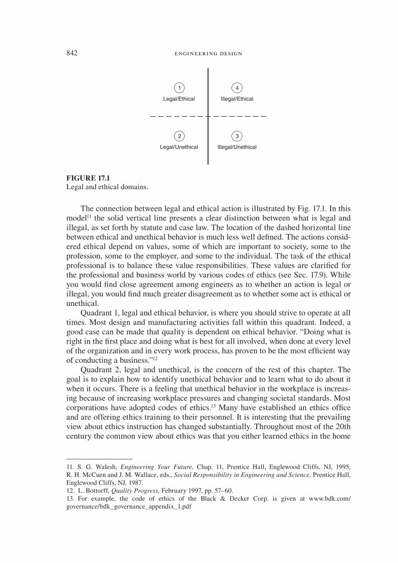
842 engineering design
The connection between legal and ethical action is illustrated by Fig. 17.1. In this model 11 the solid vertical line presents a clear distinction between what is legal and illegal, as set forth by statute and case law. The location of the dashed horizontal line between ethical and unethical behavior is much less well deE ned. The actions consid-ered ethical depend on values, some of which are important to society, some to the profession, some to the employer, and some to the individual. The task of the ethical professional is to balance these value responsibilities. These values are clariE ed for the professional and business world by various codes of ethics (see Sec. 17.9). While you would E nd close agreement among engineers as to whether an action is legal or illegal, you would E nd much greater disagreement as to whether some act is ethical or unethical.
Quadrant 1, legal and ethical behavior, is where you should strive to operate at all times. Most design and manufacturing activities fall within this quadrant. Indeed, a good case can be made that quality is dependent on ethical behavior. “Doing what is right in the E rst place and doing what is best for all involved, when done at every level of the organization and in every work process, has proven to be the most efE cient way of conducting a business.” 12
Quadrant 2, legal and unethical, is the concern of the rest of this chapter. The goal is to explain how to identify unethical behavior and to learn what to do about it when it occurs. There is a feeling that unethical behavior in the workplace is increas-ing because of increasing workplace pressures and changing societal standards. Most corporations have adopted codes of ethics. 13 Many have established an ethics ofE ce and are offering ethics training to their personnel. It is interesting that the prevailing view about ethics instruction has changed substantially. Throughout most of the 20th century the common view about ethics was that you either learned ethics in the home
Legal/Ethical Illegal/Ethical
1 4
Legal/Unethical Illegal/Unethical
2 3
FIGURE 17.1
Legal and ethical domains.
11. S. G . Walesh , Engineering Your Future, Chap. 11, Prentice Hall, Englewood Cliffs, NJ , 1995 ; R. H . McCuen and J. M . Wallace , eds., Social Responsibility in Engineering and Science, Prentice Hall, Englewood Cliffs, NJ , 1987 . 12. L . Bottorff , Quality Progress, February 1997 , pp. 57–60 . 13 . For example, the code of ethics of the Black & Decker Corp. is given at www.bdk.com/governance/bdk_governance_appendix_1.pdf
die37039_ch17.indd 842 2/25/08 7:21:05 PM

chapter 17: Legal And Ethical Issues In Engineer ing Design 843
when you were growing up, or it was too late. This is changing today to a view that ethics is a teachable subject that can be learned by just about everyone.
Quadrant 3, illegal and unethical, is the sector where “go-to-jail” cards are distributed. In general, most illegal acts also are unethical.
Quadrant 4, illegal and ethical, is a relatively rare event. An example could be an engineer who had signed a secrecy agreement with an employer, but then found that the employer had been engaged in producing a product that was very hazardous to the general public. Unable to get attention focused on the problem within the company, the engineer goes to the press to warn the public. The engineer has breached a con-tract, but in what is believed to be a highly ethical cause. Such a person would be called a whistle blower; see Sec. 17.10.1.
17.9 CODES OF ETHICS
We start by making a distinction between morality and professional ethics. Morality refers to those standards of conduct that apply to all individuals within society rather than only to members of a special group. These are the standards that every rational person wants every other person to follow and include standards such as the following:
Respect the rights of others. Show fairness in your dealings with others. Be honest in all actions. Keep promises and contracts. Consider the welfare of others. Show compassion to others.
Note that each of these standards of conduct is based on the italicized values. By professional ethics we mean those standards of conduct that every member of
a profession expects every other member to follow. These ethical standards apply to members of that group simply because they are members of that professional group. Like morality, standards of ethical conduct are value-based. Some values that are per-tinent to professional ethics include: 14
Honesty and truth Honor —showing respect, integrity, and reputation for achievement Knowledge —gained through education and experience Ef! ciency —producing effectively with minimum of unnecessary effort Diligence —persistent effort Loyalty —allegiance to employer’s goals Con! dentiality —dependable in safeguarding information Protecting public safety and health
Note that some of these values are directed toward the employer (e.g., diligence), some toward the customer (e.g., conE dentiality), some toward the profession (e.g., honor),
●
●
●
●
●
●
●
●
●
●
●
●
●
●
14. R. H . McCuen , Ethics Education Program of the Institute for Professional Practice, Verona, NJ , 1998 .
die37039_ch17.indd 843 2/25/08 7:21:06 PM

844 engineering design
and some toward society (e.g., public health and safety). These values re> ect the pro-fessional’s value obligations.
17.9.1 Profession of Engineering
The members of a profession are involved in an intellectual effort that requires special training that beneE ts society. Collectively, a group of people form a true profession only as long as they command the respect of the public and inspire conE dence in their integrity and a belief that they are serving the general welfare.
The nature of professional service varies widely. The physician, lawyer, and cler-gyman have direct, individual relations with their clients, but an engineer usually is salaried in someone else’s employ. About 95 percent of engineers work for either in-dustry or government, and only a small, but important, percentage is in direct contact with the public as consulting engineers. Thus, the service aspect of engineering may be less obvious to the general public than in other professions.
The peculiarities of the engineering profession as compared with the professions of law and medicine carry over into the area of ethics. Because engineering lacks the homogeneous character of such professions as law and medicine, it is not surprising to E nd that there is no widely accepted code of engineering ethics. Most professional societies have adopted their own codes, and ABET and NSPE have adopted broader-based ethical codes. 15 Again, because engineers who are employees of either business or government are in the great majority, they face ethical problems that self-employed professionals avoid. These arise from the con> ict between the engineer’s desire to gain a maximum proE t for the employer (and thus achieve recognition and promotion) and the desire to adhere to a standard of ethics that places the public welfare ahead of corporate proE t. For example, what can an employed engineer 16 do to expose and cor-rect the corrupt practices of an employer? What should an engineer do if employed in a business atmosphere in which kickbacks and bribes are an accepted practice?
17.9.2 Codes of Ethics
Strong parallels exist between problem solving in design and in ethical decision making. 17 In both instances, a uniquely correct solution or response is rarely possi-ble. However, some solutions are better than others, and some solutions are clearly unacceptable.
To provide guidance on how to behave in situations with ethical implications, each engineering professional society has published a code of ethics. The Code of Ethics for the American Society of Mechanical Engineers is given in Fig. 17.2. Note that the
15 . ABET is the Accreditation Board for Engineering and Technology, the professional organization that evaluated and accredits engineering and technology curricula in the United States. NSPE is the National Society of Professional Engineers. 16. T. S . Perry , IEEE Spectrum, pp. 56–61 , September 1981 . 17. C . Whitbeck , Ethics in Engineering Practice and Research, Cambridge University Press, New York , 1998 , pp. 55–66 .
die37039_ch17.indd 844 2/25/08 7:21:06 PM

chapter 17: Legal And Ethical Issues In Engineer ing Design 845
CODE OF ETHICS OF ENGINEERS
The Fundamental Principles
Engineers uphold and advance the integrity, honor and dignity of the engineering profession
by:
I. using their knowledge and skill for the enhancement of human welfare;
II. being honest and impartial, and serving with fidelity their clients (including
their employers) and the public; and
III. striving to increase the competence and prestige of the engineering profession.
The Fundamental Canons
1. Engineers shall hold paramount the safety, health and welfare of the public
in the performance of their professional duties.
2. Engineers shall perform services only in the areas of their competence; they
shall build their professional reputation on the merit of their services and
shall not compete unfairly with others.
3. Engineers shall continue their professional development throughout their
careers and shall provide opportunities for the professional and ethical
development of those engineers under their supervision.
4. Engineers shall act in professional matters for each employer or clients as
faithful agents or trustees, and shall avoid conflicts of interest or the
appearance of conflicts of interest.
5. Engineers shall respect the proprietary information and intellectual property
rights of others, including charitable organizations and professional societies
in the engineering field.
6. Engineers shall associate only with reputable persons or organizations.
7. Engineers shall issue public statements only in an objective and truthful
manner and shall avoid any conduct which brings discredit upon the
profession.
8. Engineers shall consider environmental impact and sustainable development
in the performance of their professional duties.
9. Engineers shall not seek ethical sanction against another engineer unless
there is good reason to do so under the relevant codes, policies and
procedures governing that engineer’s ethical conduct.
10. Engineers who are members of the Society shall endeavor to abide by the
Constitution, By-Laws and policies of the Society, and they shall disclose
knowledge of any matter involving another member’s alleged violation of this
code of Ethics or the Society’s Conflicts of interest policy in a prompt,
complete and truthful manner to the chair of the Committee and Ethical
Standards and Review.
FIGURE 17.2
The Code of Ethics of ASME International. http://E les.asme.org/ASMEORG/ Governance/3675.pdf
die37039_ch17.indd 845 2/25/08 7:21:06 PM

846 engineering design
code is rather brief and quite general in its statements and that it is heavily oriented toward values. It is not a list of do’s and don’ts. The three fundamental principles iden-tify goals for the ethical behavior of engineers. Use your knowledge as an engineer for the good of humanity. Do it in an honest and impartial way. Work to increase the competence of the profession of engineering. The ten fundamental canons get a bit more speciE c, but they still emphasize value statements and leave many things unsaid. This generality is intentional in well-conceived codes of ethics.
The canons 18 present the general duties of an ethical engineer. They start by rein-forcing the point that the safety, health, and welfare of the public is the E rst responsi-bility of the engineer. Next the canons charge engineers to work only in areas of their competence. The greater our competence, the better we will be able to protect public safety. Recognition of your real competencies is an important attribute. One should work to improve and expand their competence (canon 3), but also know when it is im-portant to bring in other expertise to work on a design. After all, that is why we have design teams. While it is not speciE cally stated in canon 3, the wording implies that maintaining professional competency applies not just to technical competency but it also to competency in knowledge of ethics and values.
Canon 4 charges engineers to act professionally with respect to the employer or client as faithful agents or trustees. This implies that the engineer places high impor-tance on the values of loyalty, conE dentiality, efE ciency, and diligence. The second part of this canon talks about avoiding con" icts of interest, or the appearance of such con> ict. A person is in a position of con> ict of interest when he or she is in a posi-tion to personally beneE t from actions under his or her in> uence, especially when the employer is unaware of this beneE t. For example, a design engineer who owns considerable stock in a startup company would be in con> ict of interest if he speciE ed that company’s product in his new design. Often a con> ict of interest is impossible or impractical to avoid. In this case, the best practice is to make it known to everyone involved. For example, persons serving on study committees of the National Research Council are asked to disclose any potential con> icts of interest. You might have large stock holdings in your company, yet your expertise is vital to the study that is to be un-dertaken. Your con> ict would be made part of the public record, and you would need to excuse yourself from deliberations if they ever came close to your area of con> ict.
Avoiding the appearance of con> ict of interest is as important as avoiding the con-> ict itself. Some areas that could get you in trouble are hiring relatives or close friends, accepting expensive gifts from vendors or customers, accepting a paid trip to a confer-ence from a supplier, or owning large blocks of stock in a competitor of your company.
In another example of con> ict of interest, a law E rm is forbidden by the code of ethics for lawyers to represent both parties in a dispute, even if the lawyer is asked to represent the second party in a case unrelated to the E rst dispute. 19 This part of the code arises from the adversarial nature of the legal system and the role that law-yers play therein. It is interesting to note that none of the engineering ethics codes would prevent a company from designing plastics plants for two directly competing
18 . A canon is an ecclesiastical or secular rule or law.
19. C . Whitbeck , op. cit.
die37039_ch17.indd 846 2/25/08 7:21:07 PM
chapter 17: Legal And Ethical Issues In Engineer ing Design 847
companies as long as conE dentiality was upheld. This points out that codes of ethics can differ signiE cantly between professions.
The E fth canon emphasizes the importance of intellectual property in engineer-ing practice by admonishing the engineer to respect proprietary and intellectual prop-erty. Cannon 6 is self-explanatory. Nothing is more important over the long terms than your reputation for having high ethical standards. The old adage, we are known
by the company we keep applies here. Canon 7 has many implications. It charges the engineer to be objective and truth-
ful in professional reports, statements, and public testimony. Engineers may express publicly a professional opinion on technical subjects only when that opinion is founded on adequate knowledge and competence in the subject matter. When making a public statement, any payments you may have received from interested parties to make the statement must be disclosed.
Canon 8 places emphasis on consideration of environmental and sustainability is-sues in the engineer’s work. This is a new addition to the canon. Canon 9 admonishes the engineer to be careful before bringing ethical charges against another engineer. Canon 10 reminds the engineer that a member of ASME is obligated to follow the other bylaws and policies of the organization. Also, it is their duty to report any ob-served violation of the Code of Ethics by a member.
The fundamental principles and canons are very general This enables them to be applied in a wide variety of situations. To assist the engineer in using the Code of Ethics, most professional societies publish guidelines for their interpretation. For example, we give some excerpts from the ASME Criteria for Interpretation of the Canons. 20
Canon 2. Engineers shall not request, propose, or accept professional commissions on a contingent basis if, under the circumstances, their professional judgments may be compromised.
Canon 4. Engineers shall not solicit or accept E nancial or other valuable consider-ation, for specifying products or material or equipment suppliers, without disclo-sure to their clients or employers.
Canon 4. Engineers shall admit their own errors when proven wrong and refrain from distorting or altering the facts to justify their mistakes or decisions.
Canon 8. Engineers shall concern themselves with the impact of their plans and designs on the environment. When the impact is a clear threat to heath or safety of the public, then the guidelines for this Canon revert to those of Canon 1.
Four reasons why engineers should support their profession’s Code of Ethics can be presented. 21 First, supporting the Code helps protect engineers from being harmed by what other engineers do. Second, the Code helps ensure to each engineer a work environment in which refusing to perform an unethical directive becomes easier to do. One can point to the Code in support of your position. Third, supporting the Code helps to make engineering a profession about which you need feel no morally justiE ed embarrassment. Finally, supporting the Code is the professional thing to do.
●
●
●
●
20 . http://E les.asme.org/asmeorg/NewsPublicPolicy/Ethics/10938.doc 21. M . Davis , Thinking Like an Engineer, Oxford University Press, New York , 1998 , pp. 59–60 .
die37039_ch17.indd 847 2/25/08 7:21:07 PM

848 engineering design
A young engineer on active duty with the Air Force discovers that a component used in three aircraft is overdesigned. A special adapter, costing several hundred dollars, is required for every component. The original purpose of the adapter was to permit the component to be used with a certain aircraft, but that aircraft now has been phased out of service. Thus, the adapter is redundant. The engineer tries to get the speciE cation changed to eliminate the adapter, but she is told that the “system” will not permit this.
The resourceful engineer then submits the proposal through the suggestion system of the maintenance depot where she is assigned. She receives a phone call from a staff member informing her that as a military ofE cer she cannot receive a monetary award for suggestions. The advice is given that she add a civil service engineer to the suggestion, and that they agree to split the award.
The potential for monetary reward through the suggestion system is rather great, but to do as suggested would be unethical. It would be dishonest and would not show integrity. She submits the suggestion as originally formulated, forgoing an award that could exceed $100,000. Her reward, as a military ofE cer, was dinner for two at the ofE cer’s club, and the start of a career with a reputation for high ethi-cal behavior.
22. R. H . McCuen , Issues in Engineering—Jnl. of Prof. Activities, ASCE, vol. 107, no. E12, pp. 111–120 , April 1981 .
17.9.3 Extremes of Ethical Behavior
Ethical theory considers two extreme types of behavior. Altruism is a form of moral behavior in which individuals act for the sake of other people’s interests. Ethical altru-ism is the view that individuals ought to act with each others’ interests in mind. This is the viewpoint best summarized by the Golden Rule: Do unto others as you would have others do unto you. Egoism is a form of moral behavior in which individuals act for their own advantage. Ethical egoism is the view that individuals ought always to act to satisfy their own interests. 22 Most day-to-day practice of engineering is done in the individual’s self-interest and is not in con> ict with the codes of ethics. However, the codes of ethics are meant to alert the practicing professional that he or she has altruistic obligations that must be properly balanced with self-interest.
17.10 SOLVING ETHICAL CONFLICTS
It is probably safe to say that every engineer must resolve at least one ethical dilemma over the duration of his or her career. If the engineer mishandles the situation, his or her career can be damaged even in cases where he or she is trying to do the right thing. Therefore, it is important to know how to handle ethical con> icts and to have thought about con> ict resolution before being confronted by a problem. A difE cult
die37039_ch17.indd 848 2/25/08 7:21:07 PM

chapter 17: Legal And Ethical Issues In Engineer ing Design 849
TABLE 17.2
Procedure for Solving Ethical ConS icts
I. Internal appeal option
A. Individual preparation
1. Maintain a record of the event and details
2. Examine the company’s internal appeals process
3. Be familiar with the state and federal laws that could protect you
4. Identify alternative courses of action
5. Decide on the outcome that you want the appeal to accomplish
B. Communicate with your immediate supervisor
1. Initiate informal discussion
2. Make a formal written appeal
3. Indicate that you intend to begin the company’s internal process of appeal
C. Initiate appeal through the internal chain of command
1. Maintain formal contacts as to where the appeal stands
2. Formally inform the company that you intend to pursue an external solution
II. External appeal option
A. Individual actions
1. Engage legal counsel
2. Contact your professional society
B. Contact with your client (if applicable)
C. Contact the media
R. H . McCuen , Hydrologic Analysis and Design, 2d ed., Prentice Hall, Englewood Cliffs,
NJ , 1998 .
problem for engineers arises from their dual obligation to serve diligently and with loyalty both their employer and society. The vast majority of businesses aim to be honest and responsible corporate citizens, but the con> ict between proE t and societal good is potentially always present. What should you do when confronted by an ethical con> ict where it is obvious that you have competing value responsibilities?
Ethical decision making is not easy. However, the chances for successfully resolv-ing an ethical con> ict can be greatly increased by following a systematic procedure. Table 17.2 presents one set of guidelines that will help ensure meeting one’s profes-sional responsibilities. Except under the unusual circumstances of imminent danger to the public, it is important that all internal steps should be explored before seeking op-tions outside of the organization. The process of seeking resolution to an ethical con-> ict within the organization is usually handled through an appeals process within man-agement or by the complaint process through the ofE ce of the ombudsman or the ethics ofE cer. Seeking resolution outside of the organization is usually called whistleblowing . Table 17.2 gives a step-by-step procedure for resolving an ethical con> ict, or any con-> ict for that matter, through an internal appeals process and external to your company.
The steps that the individual should take in preparation for disclosure of unethi-cal behavior are straightforward. Once you have studied and documented the facts and formulated a plan for appeal, you should discuss the matter with your immediate supervisor. Failure to fully communicate your concerns to your immediate supervisor
die37039_ch17.indd 849 2/25/08 7:21:07 PM
850 engineering design
or secretly going over his or her head to higher levels is viewed as disloyalty and will be viewed negatively by all involved, even your supervisor’s superior. It will also de-crease the likelihood of a favorable resolution of the con> ict. Often the value issue will be resolved by communicating with the immediate supervisor. However, if after fully discussing the issue with your supervisor, you feel that your supervisor is not willing or able to take appropriate action, then inform your supervisor in writing of your intention to appeal beyond that level.
The process of appealing an ethical con> ict within the company is usually similar to the process of interacting with your immediate supervisor on the issue. You should have the facts and a plan of how you would like to see the issue resolved. Formal steps should follow informal discussions, and steps within the appeal chain should not be bypassed. If the internal appeal does not resolve the ethical con> ict, then you should notify the company that you intend to continue with an external review of the problem.
Before expressing any public concern, legal advice should be obtained. A lawyer can identify courses of action and legal pitfalls in your external appeal. While lawyers understand the legal issues, they may not have the technical background to evalu-ate the technical adequacy of your arguments. For this reason it might be helpful to involve an engineering professional society as an impartial judge of your arguments. Engineering societies vary widely in their willingness to become involved in these kinds of activities.
If your company worked for a client in the issue about which you are concerned, then the client should be approached before going public. The client may pressure your company to resolve the issue internally, or the client may provide the resources to obtain an unbiased review of the issue.
The last resort is public disclosure by contacting the press and news TV. This is often called whistleblowing.
17.10.1 Whistleblowing
Whistleblowing is the act of reporting on unethical conduct within an organization to someone outside of the organization in an effort to discourage the organization from continuing the activity. In the usual case the charges are made by an employee or former employee who has been unable to obtain the attention of the organization’s management about the problem. Sometimes whistleblowing is conE ned to within the organization, where the whistleblower’s supervision is bypassed in an appeal to higher management. An important issue is to determine the conditions under which engineers are justiE ed in blowing the whistle. DeGeorge 23 suggests that it is morally permissible for engineers to engage in whistleblowing when the following conditions are met:
The harm that will be done by the product to the public is considerable and serious. Concerns have been made known to their superiors, and getting no satisfaction from their immediate superiors, all channels have been exhausted within the cor-poration, including the board of directors.
1.2.
23. R. T . DeGeorge , Business and Prof. Ethics Jnl., Vol. 1, pp. 1–14 , 1981 .
die37039_ch17.indd 850 2/25/08 7:21:08 PM

chapter 17: Legal And Ethical Issues In Engineer ing Design 851
The whistleblower must have documented evidence that would convince a reason-able, impartial observer that his or her view of the situation is correct and the com-pany position is wrong. There must be strong evidence that releasing the information to the public would prevent the projected serious harm.
Clearly a person engaging in whistleblowing runs considerable risk of being la-beled a malcontent or of being charged with disloyalty, and possibly being dismissed. The decision to blow the whistle requires great moral courage. Federal government employees have won protection under the Civil Service Reform Act of 1978, but pro-tection under state laws or active support from the engineering professional societies is still spotty. Some farsighted companies have established the ofE ce of ombudsman or an ethics review committee to head off and solve these problems internally before they reach the whistleblowing stage. Additional information can be found on the web pages of the National Whistleblower Center. 24
17.10.2 Case Studies
Ethics is best taught by looking at real-life situations through case studies. From time to time major incidents occur that catch the public’s attention, and these are recorded for posterity in the engineering ethics texts. Prominent examples are the space shut-tle Challenger tragedy, 25 the Bay Area Rapid Transit (BART) 26 control system fail-ure, and the meltdown of the Chernobyl nuclear reactor. 27 Entire areas of technology and society are the subjects of continuing ethical discussions—for example, genetic engineering. Environmental issues 28 and questions of scientiE c fraud and integrity in doing research 29 are also prominent areas for discussion.
While these major incidents and cutting-edge activities get most of the attention, the likelihood that the average engineer will be involved heavily in such cases is small. A more typical ethical situation would be:
Should I authorize the release of production parts that are only marginally out of speciE cation?
Should I condone the use of pirated design software? What should I do about the fact that my boss has in> ated my credentials on the résumé that went out with the last proposal?
3.
4.
●
●
●
24 . www.whistleblowers.org 25. R. L. B . Pinkus et al., Engineering Ethics: Lessons Learned from the Space Shuttle, Cambridge University Press, New York , 1997 ; C . Whitbeck , op. cit., Chap. 4. 26. S. H . Unger , Controlling Technology: Ethics and the Responsible Engineer, 2d ed., John Wiley & Sons, New York , 1994 , pp. 20–25 . 27. S. H . Unger , op. cit., pp. 77–91 . 28. P. A . Vesilind and A. S . Gunn , Engineering, Ethics, and the Environment, Cambridge University Press, New York , 1998 . 29. C . Whitbeck , op. cit., Chaps. 6, 7, 9, 10.
die37039_ch17.indd 851 2/25/08 7:21:08 PM

852 engineering design
Fortunately, the number and diversity of case studies that deal with day-to-day ethical problems is growing. In recognition of the importance it places on ethics, the National Academy of Engineering (NAE) has established an Engineering Ethics Center.30 This website combines case studies, educational material, and reference ma-terial on engineering ethics previously located in many diverse places.
17.11
SUMMARY
Engineers mostly work in the business world, and they are therefore required to per-form their duties within the laws of the nation. But more than this, engineering is a profession that is critical to the advancement of society. How engineers do their jobs determines what kind of world future generations will enjoy. Thus, the practice of engineering without question will involve you in making ethical judgments. Most will be small in nature, involving your relationship with your management and your fellow engineers, but others could be momentous, affecting the safety of a city.
The law is a formalized code of conduct describing what society feels is the proper way to behave. Statutory law is created by a federal or state legislative body. Case law arises from the decisions of the courts. Ethics is the study of human conduct that lays out the moral ground rules based on society’s values. Ethical conduct is the
30 . www.onlineethics.org
A consulting engineer is hired by the county to investigate a bridge collapse. In the course of his investigation he examines a bridge of similar design and E nds that it is only marginally safe. He contacts the county engineer to tell him about this dis-covery. The county ofE cial tells him that they know about this condition and that they hope to repair it in the next budget year. However, they must keep the second bridge open because to close it would increase the response time of emergency ve-hicles by about 30 minutes. What should the consulting engineer do?
He goes back to the marginal bridge and makes a more thorough investigation, taking photographs and measurements. He E nds the situation more dangerous than he E rst thought. Back at the ofE ce he makes some calculations and prepares a brief report. He asks for a meeting with the county engineer and lays out the case for closing the bridge. The county engineer is impressed, but points out the political implications of closing the bridge. He suggests a joint meeting with the county su-pervisor. They meet with the county supervisor, who is impressed with the severity of the situation, and the spirit of civic duty shown by the engineer. They agree to post the bridge to forbid general trafE c, but to leave it open to emergency vehicles. The county supervisor schedules a press conference to which he invites the con-sulting engineer as an honored guest.
die37039_ch17.indd 852 2/25/08 7:21:09 PM

chapter 17: Legal And Ethical Issues In Engineer ing Design 853
behavior that is desired by society and is separate from the minimum standards of the law.
Engineers should be familiar with contracts and liability, especially product liability. A contract is an agreement between two parties to do or not to do something. It consists of an offer, an acceptance of the offer, and a consideration, the exchange of something of value. A contract is discharged when the agreement has been performed to the satisfaction of both parties. A breach of contract occurs when one party fails to perform its part of the contract.
Liability means being bound or obligated to pay damages or restitution. Two com-mon ways of incurring liability are breaching a contract or committing a tort. A tort is a civil wrong committed against a person, or the business, property, or reputation that causes damage. Common examples of torts are fraud, misrepresentation, negligence, and product liability.
Product liability is the legal action by which an injured party seeks to recover damages for personal injury or property loss from the producer or seller of a product. The law under which product liability is tried has evolved to a standard of strict prod-uct liability. Under this theory of law, the plaintiff must prove that: (1) the product was defective and unreasonably dangerous, (2) the defect existed at the time the product left the defendant’s control, (3) the defect caused the harm, and (4) the harm is appro-priately assignable to the identiE ed defect. Previously, manufacturers were liable only when they could be proved negligent or unreasonably careless.
To protect against product liability suits, the design procedures described in Secs. 13.8, 14.4, 14.5, 14.6, and 14.7 must be followed. In addition, documentation of these design methods and of testing and quality activities is vital. There should be an active product safety committee to see that every step is taken to ensure the design and pro-duction of safe products. Finally, it may be a wise business decision to obtain insur-ance protection for product liability suits and product recall expenses.
While the boundary between legal and illegal acts is generally well deE ned by the law, the distinction between what is ethical and what is unethical is much less well deE ned. Professional engineering societies provide guidance by means of codes of ethics. Different individuals respond differently, depending on their value systems. Engineering is a profession, and as such, you are bound by the ethical standards of the profession. It does not matter whether you have individually made that agreement. The profession expects you to behave in a certain ethical way. These rules of conduct are laid down in the code of ethics of each professional engineering society. The existence of a code of ethics is important to you because it gives you an authoritative standard to fall back on if you are engaged in a serious ethical con> ict in the workplace.
Table 17.3 suggests typical ethical questions associated with different steps in the product design process. 31
It is not inconceivable that you will be involved in a serious ethical con> ict some-time in your career. This often arises from the competing value responsibilities that engineers have, such as loyalty and diligence to both their employer and the good of society. If such a con> ict does arise, it is important to try to resolve the disagreement
31. M. W . Martin and R . Schinzinger , Ethics in Engineering, 3d ed., McGraw-Hill, New York , 1996 .
die37039_ch17.indd 853 2/25/08 7:21:09 PM

854 engineering design
internally in your organization. Follow to the letter the prescribed appeal procedure, and document everything. If you must go outside of the organization, obtain compe-tent legal counsel.
NEW TERMS AND CONCEPTS
TABLE 17. 3
Typical Ethical Questions Associated with Product Design
Steps in Product Design Possible Ethical Questions
Market study Is the study unbiased, or has it been embellished to attract investors or management support?
Conceptual design Will the product be useful or will it be just a gimmick?
Embodiment design Does the design team have sufE cient expertise to properly judge whether computer programs are giving reliable results? Have any patents been violated?
Detail design Has checking of results been done?
Manufacturing Is the workplace safe and free of environmental hazards? Is enough time allowed to do quality work?
Product use Is the product safe to use? Are users informed of possible hazards?
Retirement from service Has the design allowed for recycling or reuse?
Altruism Canons of ethics Code of ethics Con> ict of interest Express contract Fraud
Implied contract Intellectual property Liability Negligence Product liability Statutes
Strict liability Tort law Trade dress Utility patent Values Whistleblower
BIBLIOGRAPHY
Law and the Engineer
Blinn , K. W .: Legal and Ethical Concepts in Engineering, Prentice Hall, Englewod Cliffs, NJ , 1989 .
Liuzzo , A , and J. G . Bonnice : Essentials of Business Law, 6th ed., McGraw-Hill, New York , 2007 .
Engineering Law, Design Liability, and Professional Ethics, Professional Publication, Belmont, CA , 1983 .
Product Liability
Brown , S ., I . LeMay , J . Sweet , and A . Weinstein , eds.: Product Liability Handbook: Preven-
tion, Risk, Consequence, and Forensics of Product Failure, Van Nostrand Reinhold, New York , 1990 .
die37039_ch17.indd 854 2/25/08 7:21:09 PM

chapter 17: Legal And Ethical Issues In Engineer ing Design 855
Hunziker , J. R ., and T. O . Jones : Product Liability and Innovation, National Academy Press, Washington, DC , 1994 .
Smith , C. O .: Products Liability: Are You Vulnerable? Prentice Hall, Englewood Cliffs, NJ , 1981 .
Engineering Ethics
Budinger , T. F ., and M. D . Budinger , Ethics of Emerging Technology, John Wiley & Sons, Hoboken, NJ , 2006 .
Davis , M .: Thinking Like an Engineer: Studies in the Ethics of a Profession, Oxford University Press, Oxford , 1998 .
Harris , C. E ., M. S . Pritchard , and M . Rabins : Engineering Ethics: Concepts and Cases, 3d ed., Thomson-Wadsworth Publishing Co., Belmont, CA , 2005 .
Martin , M. W .: Ethics in Engineering, 4th ed., McGraw-Hill, New York , 2005 . Unger , S. H .: Controlling Technology. Ethics and the Responsible Engineer, 2d ed., John
Wiley & Sons, New York , 1994 . Whitbeck , C .: Ethics in Engineering Practice and Research, Cambridge University Press,
New York , 1998 .
PROBLEMS AND EXERCISES
17.1. John Williams, a professional engineer, agrees to testify as an expert witness for the E rm of Jones & Black in a court case. In return, the E rm promises to pay Williams $1500 plus expenses for his services.
(a) Is this a lawful contract? State the reasons for your decision. (b) Suppose Williams agrees to accept $2500 if Jones wins, but only expenses if
Jones loses. Is this a lawful contract? State your reasons.
17.2. ABC Electric agreed by fax on Monday to buy 100 fractional-horsepower motors for $3000 from Amalgamated Electric. On Wednesday the purchasing agent from ABC calls and says he is canceling the order. Amalgamated says the motors have already been shipped and they want their money.
(a) What is the legal responsibility of ABC Electric in this transaction? (b) Would it have been any different if the motors had not already been shipped?
17.3. A car designer speciE ed steel bolts of the highest quality and strength when designing a connection for the front-end steering rods. The manufacturer of the bolts used an inadequate sampling plan for inspecting the bolts, and several defective bolts caused failure of the steering mechanism. Several deaths resulted, and there was a major product recall. Discuss the liability of the designer, the auto company, and the bolt manufacturer.
17.4. Read the story of the failure of the General Electric refrigerator with the revolution-ary rotary compressor (Wall Street Journal, May 7, 1990, p. A1, A5). What lessons does this teach us about product design? What implications does it have for product liability?
die37039_ch17.indd 855 2/25/08 7:21:09 PM

856 engineering design
17.5. Aristotle put forth the precept that humanity should follow four virtues: (1) prudence, (2) justice, (3) fortitude, and (4) temperance. DeE ne each virtue broadly and give ex-amples of ethical behavior for each virtue.
17.6. Make a list of business practices that signal whether an organization is an ethical cor-poration. What role does the CEO of the corporation play in this?
17.7. We are in a period where the desire for steady increase in corporate earnings, driven to a large degree by the stock market, sometimes causes management to require layoffs even when proE ts are good. Discuss the ethics of this from the viewpoint of both cor-porate management and the individual engineer.
17.8. Imagine what it would be like if there were no codes of ethics for engineers. What would be the consequences?
17.9. A trend in sports equipment has been to improve the players’ performance by intro-ducing new products. Examples are the graphite-composite shaft and titanium head in golf drivers, lighter-weight composite tennis rackets with a larger “sweet” spot, and an aluminum baseball bat with built-in damping. Discuss the ethics of com-pensating for personal inadequacies in performance with technology in competitive sports.
17.10. Discuss the ethics of the following situation: You are a design engineer for the Ajax Manufacturing Co., a large multiplant producer of plastic parts. As part of your em-ployment, you were required to sign a secrecy agreement that prohibits divulging in-formation that the company considers proprietary.
Ajax has modiE ed a standard piece of equipment that greatly increases the efE -ciency in cooling viscous plastic slurries. The company decides not to patent the devel-opment but instead to keep it as a trade secret. As part of your regular job assignment, you work with this proprietary equipment and become thoroughly familiar with its enhanced capabilities.
Five years later you leave Ajax and go to work for a candy manufacturer as chief of production. Your new employer is not in any way in competition with Ajax. You quickly realize that Ajax’s trade secret can be applied with great proE t to a completely different machine used for cooling fudge. You order the change to be made. Discuss the ethics.
17.11. Discuss the ethics in the following situation: You have been on the job for nine months as an assistant research engineer working with a world-famous authority on heat trans-fer. It is an ideal job, because you are learning a great deal under his sympathetic tute-lage while you pursue an advanced degree part-time.
You are asked to evaluate two new > ame-retardant paints A and B. Because of late delivery of some constituents of paint A, the test has been delayed and your boss has been forced to make a tentative recommendation of paint A to the design group. You are asked to make the after-the-fact tests “for the record.” Much to your surprise, the tests show that your boss was wrong and that formulation B shows better > ame resistance. However, a large quantity of paint A already has been purchased. Your boss asks you to “fudge the data” in favor of his original decision, and since there is reason-able possibility that your data were in error, you reluctantly change them to favor his decision. Discuss the ethics.
die37039_ch17.indd 856 2/25/08 7:21:10 PM

chapter 17: Legal And Ethical Issues In Engineer ing Design 857
17.12. A new development in the intellectual property arena is the presence of “patent trolls.” These are small organizations, usually just a clever inventor and a patent attorney, who buy up patents or hold the inventor’s patents in a fast-moving area of technology, such as information technology. The trolls have no plans to make a product based on their patents. Instead they lie in wait, hoping to snare an unwitting manufacturer that infringes on one of their patents and to demand an outrageous royalty payment. Research in Motion, RIM, the producer of the hand-held wireless device called Black-berry, was sued in 2005 by a troll named NTF.
Find out more about what happened in the case of RIM versus NTF and identify the societal issues involved with patent trolls.
die37039_ch17.indd 857 2/25/08 7:21:10 PM

858
18
ECONOMIC DECISION MAKING
18.1 INTRODUCTION
Throughout this book we have repeatedly emphasized that the engineer is a decision maker and that engineering design is a process of making a series of decisions over time. We also have emphasized from the beginning that engineering involves the ap-plication of science to real problems of society. In this authentic context, one cannot escape the fact that economics may play a role as big as, or bigger than, that of techni-cal considerations in the decision making process of design. In fact, it sometimes is said, although a bit facetiously, that an engineer is a person who can do for $1.00 what any fool can do for $2.00.
The major engineering infrastructure that built this nation—the railroads, major dams, and waterways—required a methodology for predicting costs and balancing them against alternative courses of action. In an engineering project, costs and rev-enues will occur at various points of time in the future. The methodology for handling this class of problems is known as engineering economy or engineering economic analysis. Familiarity with the concepts and approach of engineering economy gener-ally is considered to be part of the standard engineering toolkit. Indeed, an examina-tion on the fundamentals of engineering economy is required for professional engi-neering registration in all disciplines in all states.
The chief concept in engineering economy is that money has a time value. Pay-ing out $1.00 today is more costly than paying out $1.00 a year from now. A dollar invested today is worth a dollar plus interest a year from now. Engineering economy recognizes the fact that the use of money is a valuable asset. Money can be rented in the same way one can rent an apartment, but the charge for using it is called interest rather than rent. This time value of money makes it more proM table to push expenses into the future and bring revenues into the present as much as possible.
Before proceeding into the mathematics of engineering economy, it is important to understand where engineering economy sits with regard to related disciplines like
die37039_ch18.indd 858 2/25/08 7:21:28 PM

chapter 18: Economic Decision Making 859
economics and accounting. Economics generally deals with broader and more global issues than engineering economy, such as the forces that control the money supply and trade between nations. Engineering economy uses the interest rate established by the economic forces to solve more speciM c and detailed problems. However, it usually is a problem concerning alternative costs in the future. The accountant is more concerned with determining exactly, and often in great detail, what costs have been incurred in the past. One might say that the economist is an oracle, the engineering economist is a fortune teller, and the accountant is a historian.
18.2 MATHEMATICS OF TIME VALUE OF MONEY
If we borrow a present sum of money or principal P at a simple interest rate i , the annual cost of interest is I 5 Pi . If the loan is repaid in a lump sum F at the end of n years, the amount required is
F P nI P nPi P ni= + = + = +( )1 (18.1)
where F 5 future worth P 5 present worth I 5 annual cost of interest i 5 annual interest rate n 5 number of years
If we borrow $1000 for 6 years at 10 percent simple interest rate, we must repay at the end of 6 years:
F P ni= +( ) = + ( ) =1 1000 1 6 0 10 1600$ . $
Therefore, we see that $1000 available today is not equivalent to $1000 available in 6 years. Actually, $1000 in hand today is worth $1600 available in only 6 years at 10 percent simple interest.
We can also see that the present worth of $1600 available in 6 years and invested at 10 percent is $1000.
P
F
ni=
+=
+=
1
1600
1 0 61000
$
.$
In making this calculation we have discounted the future sum back to the present time. In engineering economy the term discounted refers to bringing dollar values back in time to the present.
18.2.1 Compound Interest
However, you are aware from your personal banking experiences that M nancial trans-actions usually use compound interest. In compound interest, the interest due at the
die37039_ch18.indd 859 2/25/08 7:21:29 PM

860 engineering design
end of a period is not paid out but is instead added to the principal. During the next period, interest is paid on the total sum.
First period:
Second period:
F P P P i
F
i1
2
1= + = +( )== +( ) + +( ) = +( ) +( ) = +( )P i iP i P i i P i1 1 1 1 1
2
Thirrd period: F P i iP i P i3
2 2 2
1 1 1= +( ) + +( ) = +( )
+( ) = +( )= +( )
1 1
1
3
i P i
n F P in
n
th period:
(18.2)
We can write Eq. (18.2) in a short notation that is convenient to use when the engi-neering economy relationships become more complex.
F P i P F P i nn
n
= +( ) = ( )1 / , , (18.3)
In Eq. (18.3) the function ( F / P, i, n ) has the meaning: Find the equivalent amount F given the amount P compounded at an interest rate i for n interest periods.
E X A M P L E 1 8 . 1 How long will it take money to double if it is compounded annually at a rate of 10 percent per year?
F P F P n F P= ( ) =/ but we want to find the d, , ,10 2 ooubling time
/( )
= ( )2 10P P F P n, ,
Therefore, the answer clearly is found in a table of single-payment compound-amount factors at the year n for which F PS 5 2.0. Examining the table in Appendix 2 we see that, for n 5 7, F PS 5 1.949 and, for n 5 8, F PS 5 2.144. Linear extrapolation gives us F PS 5 2.000 at n 5 7.2 years. We can generalize the result to establish the H nancial rule of thumb that the number of years to double an investment is 72 divided by the interest rate (expressed as an integer).
Usually in engineering economy, n is given in years and i is an annual interest rate. However, in banking circles the interest may be compounded at periods other than one year. Compounding at the end of shorter periods, such as daily, raises the effective interest rate. If we deH ne r as the nominal annual interest rate and p as the number of interest periods per year, then the interest rate per interest period is i 5 r / p and the number of interest periods in n years is pn . Using this notation, Eq. (18.2) becomes
F Pr
p
pn
= +
1 (18.4)
Note that when p 5 1, the above expression reduces to Eq. (18.2). Standard com-pound interest tables that are prepared for p 5 1 can be used for other than annual periods. To do so, use the table for i 5 r / p and for a number of years equal to p 3 n . Alternatively, use the interest table corresponding to n years and an effective rate of yearly return equal to (1 1 r / p )
p 2 1.
die37039_ch18.indd 860 2/25/08 7:21:29 PM

chapter 18: Economic Decision Making 861
TABLE 18.1
In' uence of Compounding Period on Effective Rate of Return
Frequency of
Compounding
No. Annual
Interest Periods p
Interest Rate
for Period, %
Effective Rate of
Yearly Return, %
Annual 1 12.0 12.0
Semiannual 2 6.0 12.4
Quarterly 4 3.0 12.6
Monthly 12 1.0 12.7
Continuously ` 0 12.75
If the number of interest periods per year p increases without limit, then i 5 r / p approaches zero.
F Pr
pp
pn
= +
→∞
lim 1 (18.5)
From calculus, an important limit is lim x→0 (1 1 x ) 1/ x 5 2.7178 5 e . If we let x 5 r / p ,
then
pnp
rrn
xrn= =
1
Since p 5 r / x , as p →∞, x →0, so Eq. (18.5) is rewritten as
F P x Pex
xrn
rn= +( )
=→∞
lim/
11
(18.6)
Table 18.1 shows the ind uence of the number of interest periods per year on the effective rate of return.
18.2.2 Cash Flow Diagram
Engineering economy was developed to deal with H nancial transactions taking place at various times in the future. This can be best understood in terms of cash ! ows.
Some of these will be cash ind ows (receipts), like revenue from sale of products, re-duction in operating cost, sale of used machinery, or tax savings. Others will be cash outd ows (disbursements), such as the costs incurred in designing a product, the oper-ating costs in making the product, and the periodic maintenance costs in keeping the factory running. The net cash d ow is given by
Net cash flow cash inflows receipts cash outflows disbur= ( ) − ssements( ) (18.7)
die37039_ch18.indd 861 2/25/08 7:21:29 PM

862 engineering design
Cash d ows occur frequently and take place at varying times within the time pe-riod of the problem. In the cash d ow diagram, Fig. 18.1, the horizontal axis represents time and the vertical axis is cash d ow. Cash ind ows are positive and are represented by arrows above the x-axis. Cash outd ows are negative and are below the x-axis. It has been mentioned that engineering economy is chied y concerned with assisting decision making about future H nancial decisions in an engineering project. Since future predic-tion of cash d ows is likely to be imprecise, it is not worth carefully locating each cash d ow on the diagram in time. Instead, the end-of-period convention is used in which the cash d ows within a period are assumed to occur at the end or the interest period.
18.2.3 Uniform Annual Series
In many situations we are concerned with a uniform series of receipts or disburse-ments occurring equally at the end of each period. Examples are the payment of a debt on the installment plan, setting aside a sum that will be available at a future date for replacement of equipment, and a retirement annuity that consists of a series of equal payments instead of a lump sum payment. We will let A be the equal end-of-the-period payment that makes up the uniform annual series.
Figure 18.2 shows that if an annual sum A is invested at the end of each year for 3 years, the total sum F at the end of 3 years will be the sum of the compound amount of the individual investments A
F A i A i A= +( ) + +( ) +1 1
2
and for the general case of n years,
F A i A i A i A i An n
= +( ) + +( ) + ⋅⋅ ⋅ + +( ) + +( ) +− −
1 1 1 11 2 2
(18.8 )
0 =1 2 3
01 2 3
+ 01 2 3
+ 01 2 3
FIGURE 18.2
Equivalence of a uniform annual series.
FIGURE 18.1
Cash d ow diagram.
0 1 2 3
Present Years
Time
Disbursements (costs)
4 5 6
Receipts (income)
die37039_ch18.indd 862 2/25/08 7:21:30 PM

chapter 18: Economic Decision Making 863
Multiplying by 1 1 i , we get
F i A i A i A i A in n
1 1 1 1 11 3
+( ) = +( ) + +( ) + ⋅⋅ ⋅ + +( ) + +( )− 22
1+ +( )A i (18.9)
Subtracting Eq. (18.8) from Eq. (18.9):
1 1 1 1 1 11 3 2
+( ) = +( ) + +( ) + ⋅⋅⋅+ +( ) + +( ) +−
i F A i i i in n
++( )
= +( ) + +( ) + ⋅⋅⋅+ +( ) +− −
i
F A i i in n
1 1 11 2 2
11 1
1 1
1 1
+( ) +
= +( ) −
=+( ) −
i
F A i
F Ai
i
n
n
(18.10)
Equation (18.10) gives the future sum of n uniform payments of A when the interest rate is i . This equation may also be written:
F A F A i nn
= ( )/ , , (18.11)
where F / A , i , n is the uniform-series compound amount factor that converts a series A to a future worth F .
By solving Eq. (18.10) for A , we have the uniform series of end-of-period pay-ments, that, at compound interest i , provide a future sum F .
A Fi
in
=+( ) −1 1
(18.12)
This type of calculation often is used to set aside money in a sinking fund to provide funds for replacing worn-out equipment, or for investing money to send a child to college.
A F A F i n= ( )/ , , (18.13)
where ( A / F , i , n ) is the sinking fund factor. It sets up a future fund F by investing A each interest period n at a rate i .
By combining Eq. (18.2) with Eq. (18.10), we develop the relation for the present worth of a uniform series of payments A :
P Ai
i iA P A i n
n
n=
+( ) −
+( )= ( )1 1
1/ , , (18.14)
Solving Eq. (18.14) for A gives the important relation for capital recovery:
A Pi i
iP A P i n
n
n=
+( )+( ) −
= ( )1
1 1/ , , (18.15)
die37039_ch18.indd 863 2/25/08 7:21:30 PM

864 engineering design
where ( A / P , i , m ) is the capital recovery factor. The A in Eq. (18.15) is the annual pay-ment needed to return the initial capital investment P plus interest on that investment at a rate i over n years.
Capital recovery is an important concept in engineering economy. It is important to understand the difference between capital recovery and sinking fund. Consider the following example:
E X A M P L E 1 8 . 2 What annual investment must be made at 10 percent to provide funds for replacing a $10,000 machine in 20 years?
A F A F= ( ) = ( ) =/ per, , $ , . $ .10 20 10 000 0 01746 174 60 year put into the sinking fund
What is the annual cost of capital recovery of $10,0000 at 10 percent over 20 years?
/A P A P= , ,10 20(( ) = ( ) =$ , . $ .10 000 0 11746 1174 60 per year for ccapital recovery
We see that / /A P i n A F, , ,( ) = ii n i,
. . .
( ) +
= +0 11746 0 01746 0 10000
Annual cost oof capital recovery annual cost of sinking= fund annual interest cost
$1174.60 = $174.
+
660 + 0.10 $10,000( )
With a sinking fund we put away each year a sum of money that, over n years, together with accumulated compound interest, equals the required future amount F . With capital recovery we put away enough money each year to provide for replace-ment in n years plus we charge ourselves interest on the invested capital. The use of capital recovery is a conservative but valid economic strategy. The amount of money invested in capital equipment ($10,000 in Example 18.2) represents an opportunity
cost, since we are forgoing the revenue that the $10,000 could provide if invested in interest-bearing securities.
A summary of the compound interest relationships among F, P, and A is given in Table 18.2
Table 18.2 gives relationships for a uniform series of payments or receipts. Two other series often used in engineering economy are a gradient series in which the cash d ow increases (or decreases) by a H xed increment at each time period, and a geometric series in which the cash d ow changes by a H xed percentage at each time period. 1
Using symbolic notation, as shown in Table 18.2, simpliH es writing the equations and aids in making calculations. For example, many compound interest tables do not contain a table for determining A (sinking fund factor) when F is known. However, us-ing the symbolic factors this can be obtained by simply multiplying factors.
A F A F F P F A P= ( ) = ( )( )/ / / (18.16)
1. L. T . Blank and A. J . Tarquin , Engineering Economy 6th ed., McGraw-Hill, New York , 2004 .
die37039_ch18.indd 864 2/25/08 7:21:31 PM

chapter 18: Economic Decision Making 865
18.2.4 Irregular Cash Flows
Payment at the Beginning of the Interest Period
In working with a uniform series of payments of receipts, A , it is conventional practice to assume that A occurs at the end of each period. However, sometimes a se-ries of payments begins immediately so that the payments are made at the beginning of each time period, A b .
As Fig. 18.3 shows, this is equivalent to increasing each annual payment by the interest earned in one period of the accumulation of interest. Thus, Eq. (18.10) would be written as
F A ii
ib
n
= +( ) +( ) −
11 1
(18.17)
Payments in Alternate Years
Figure 18.4 shows uniform payments in alternate years. One approach would be to consider this as three future payments and determine P as follows:
P P F P F P P F= ( ) + ( ) + ( ) =100 10 2 100 10 4 10 6 8/ / /, , , , , , 22 64 68 30 56 45 207 39. . . $ .+ + =
An alternative approach is to consider the H rst annual payment to be a future payment over two years and determine the annual payment (sinking fund factor) to produce
TABLE 18.2
Summary of Compound Interest Factors
Item Conversion Algebraic Relation Factor Factor Name
1 P to F F P i n= +( )1
( F / P,i,n ) Single payment,
compound amount factor
2 F to P P F i n= +( )1
( P / F,i,n ) Single payment, present
worth factor
3 A to P
P Ai
i i
n
n=
+( ) −
+( )1 1
1
( P / A,i,n ) Uniform payment, present worth factor
4 P to A
A Pi i
i
n
n=
+( )+( ) −
1
1 1
( A / P,i,n ) Capital recovery factor
5 A to F
F Ai
i
n
=+( ) −1 1
( F / A,i,n ) Uniform series, compound amount factor
6 F to A
A Fi
in
=+( ) −1 1
( A / F,i,n ) Sinking fund factor
die37039_ch18.indd 865 2/25/08 7:21:31 PM

866 engineering design
$100. This would then be an annual payment paid over six years, since the pay-ments are at the end of every two years, for six years total. A 5 100 (A/F, 10, 2) 5 100(0.4762) 5 $47.62)
P P A= ( ) = ( ) =47 62 10 6 47 62 4 3553 207 39. , , . . $ ./
Uniform Payments Not Extending to Time Zero
Consider the uniform payments. A extending from years 4 to 10, Fig. 18.5. To H nd the present value, P 5 A ( P / A i , 7). This present value is located at the end of year 3, because the compound interest equations for the P / A factor assume that P will be determined one interest period prior to the H rst A in the series. Then to H nd the pres-ent value at time zero, P 3 must be discounted to the present. P 5 F ( P / F , i , 3) where F 5 P 3 .
Nb 5 100 100 100 100 100
110 5 A
i 5 10%
110110 110 110
0 1 2 3 4 5 0 1 2 3 4 5
5
FIGURE 18.3
A uniform series paid at the beginning of the interest period, and the equivalent series paid at the end of the period.
FIGURE 18.5
Finding present values of a uniform series that does not extend to time zero.
0 1 2 3 4 5
A
6 7 8 9 10
100
0 1 2 3 4 5 6 0 1 2 3 4 5 6
100 100
47.62 47.62 47.62 47.62 47.62 47.625
FIGURE 18.4
Conversion of payments every two years into annual payments.
die37039_ch18.indd 866 2/25/08 7:21:32 PM

chapter 18: Economic Decision Making 867
18.3 COST COMPARISON
Having discussed the usual compound interest relations, we now are in a position to use them to make economic decisions. A typical decision is which of two courses of action is less expensive when the time value of money is considered. Generally the rate of interest to be used in these calculations is set by the minimum attractive rate of
return, MARR. This is the lowest rate of return a company will accept for investing its money. The MARR is established by the corporate H nance ofH cer based on cur-rent market opportunities for investing money or on the importance of the project to advancing the company.
18.3.1 Present Worth Analysis
When the two alternatives have a common time period, a comparison on the basis of present worth is advantageous.
E X A M P L E 1 8 . 3 Two machines each have a useful life of 5 years. If money is worth 10 percent, which machine is more economical?
A B
Initial cost $25,000 $15,000
Yearly maintenance cost 2,000 4,000
Rebuilding at end of third year — 3,500
Salvage value 3,000
Annual beneH t from better quality production 500
From the cost diagrams given on the next page we see that the cash d ows deH nitely are different for the two alternatives. To place them on a common basis for comparison, we discount all costs back to the present time.
P P A P F
A= + −( )( ) −25 000 2000 500 10 5 3000 10 5, , , , ,/ /(( )= + ( ) − ( ) =25 000 1500 3 791 3000 0 621 28 823, . . $ ,
PBB
P A P F= + ( ) + ( )=
15 000 4000 10 5 3500 10 3
15
5, , , , ,/ /
,, . . $ ,000 4000 3 791 3500 0 751 32 793+ ( ) + ( ) =
Machine A is more economical because it has the lower cost on a present worth basis. In this example we considered both (1) costs plus beneH ts (savings) due to reduced scrap rate and (2) resale value at the end of the period of useful life. Thus, we really determined
die37039_ch18.indd 867 2/25/08 7:21:33 PM

868 engineering design
the net present worth for each alternative. We should also point out that present worth analysis is not limited to the comparison of only two alternatives. We could consider any number of alternatives and select the one with the smallest net present worth of costs.
In Example 18.3, both alternatives had the same life. Thus, the time period was the same and the present worth could be determined without ambiguity. Suppose we want to use present worth analysis for the following situation:
2000
500
2000
500
2000
500
2000
500
2000
500
3000
25,000
Machine A
4000
15,000
4000 4000
3500
4000 4000
Machine B 0
18,000
Machine A PA2 = $24,529 (for i = 10%)01
4000
2
4000
500
25,000
Machine B PB3 = $31,334 (for i = 10%)01
3000
2
3000
3
3000
1500
die37039_ch18.indd 868 2/25/08 7:21:33 PM

chapter 18: Economic Decision Making 869
We cannot directly compare P A and P B because they are based on different time periods. One way to handle the problem would be to use a common 6-year period, in which we would replace machine A three times and replace machine B twice. This procedure works when a common multiple of the individual periods can be found eas-ily, but a more direct approach is to convert the present worth based on a period n 1 to an equivalent P based on n 2 by 2
P PA P i nA P i nn n2 1
1
2
=( )( )
//
, ,, ,
(18.18)
For our example, we convert P B from a 3-year time period to a 2-year period.
P PA P i nA P i n
A PB B2 1
1
2
31 33410 3
=( )( ) =
(//
/, ,, ,
,, , ))
( ) =
=A P/ , ,
, ..
$10 2
31 334 0 402110 57619
21,,867
Since P A 5 $24,529, machine B is the more economical when compared on the basis of present worth for equal time periods .
18.3.2 Annual Cost Analysis
In the annual cost method, the cash d ow over time is converted to an equivalent uni-form annual cost or beneH t. In this method no special procedures need be used if the time period is different for each alternative, because all comparisons are on an annual basis ( n 5 1).
Example Machine A Machine B
First cost $10,000 $18,000
Estimated life 20 years 35 years
Estimated salvage 0 $3000
Annual cost of operation $4000 $3000
A A PA = ( ) + = ( ) +10 000 10 20 4000 10 000 0 1175 40, , , , ./ 000 5175
18 000 3000 10 35 3000 05
=
= −( )( ) +
$, , ,A A PB / .. $10 3000 4855( ) + =
Machine B has the lower annual cost and is the more economical. Note that in cal-culating the annual cost of capital recovery for machine B we used the difference between the H rst cost and the salvage value; for it is only this amount of money that must be recovered. However, although the salvage value is returned to us, we are re-quired to wait until the end of the useful life of the machine to recover it. Therefore,
2. For a derivation of Eq. (18.18), see F. C . Jelen and J. H . Black , Cost and Optimization Engineering, 2d ed., p. 28 , McGraw-Hill, New York , 1983 .
die37039_ch18.indd 869 2/25/08 7:21:33 PM

870 engineering design
a charge for the annual cost of the interest on the investment tied up in the salvage value is made as part of the annual cost analysis.
Perhaps a more direct way to handle the case of machine B in the preceding ex-ample is to determine the equivalent annual cost based on the cash disbursements minus the annual beneH t of the future resale value.
A A P A FB = ( ) + − ( )18 000 10 35 3000 3000 10 3535
, , , , ,/ /335
18 000 0 1037 3000 3000 0 0037 4855= ( ) + − ( ) =, . . $
18.3.3 Capitalized Cost Analysis
Capitalized cost is a special case of present worth analysis. The capitalized cost of a project is the present value of providing for that project in perpetuity ( n 5 ∞). The concept was originally developed for use with public works, such as dams and water-works, that have long lives and provide services that must be maintained indeH nitely. Capitalized cost subsequently has been used more broadly in economic decision mak-ing because it provides a method that is independent of the time period of the various alternatives.
We can develop the mathematics for capitalized cost quite simply from Eq. (18.18). If we let n 2 5 ∞ and n 1 5 n, then
P PA P i n
A P i
A P i ni i
i
n
n
``
=( )( )
( ) =+( )
+
/
/
/
, ,
, ,
, ,1
1(( ) −( ) =
+( )+( ) −
=n
A P ii i
ii
1
1
1 1/ , , `
`
`
Therefore, the capitalized cost K of a present sum P is given by
K P Pi
iP K P i n
n
n= =+( )
+( ) −= ( )
`
1
1 1/ , , (18.19)
Since most tables of compound interest factors do not include capitalized cost, we need to note that
K P i n A P i n i/ /, , , ,( ) = ( ) (18.20)
In addition, the capitalized cost of an annual payment A is determined as follows:
P A P A i n K P K P i n P
A P i ni
= ( ) = ( ) =( )/ /
/from E, , , ,
, ,qq. 18.20
Substituting for dropping th
( ).
,P ee notation for and : //
i n K A P AA Pi
Ai
= ( ) ( )=
(18.21)
die37039_ch18.indd 870 2/25/08 7:21:34 PM

chapter 18: Economic Decision Making 871
E X A M P L E 1 8 . 4 The capitalized cost is the present worth of providing for a capital cost in perpetuity; that is, we assume there will be an inH nite number of renewals of the initial capital investment. Consider a bank of condenser tubes that cost $10,000 and have an average life of 6 years. If i 5 10 percent, then the capitalized cost is
K K P i n P
A P i n
i= ( ) =
( )= =/
/, ,
, ,,
.
.$10 000
0 2296
0 10222 960,
We note that the excess over the H rst cost is 22,960 2 10,000 5 $12,960. If we invest that amount for the 6-year life of the tubes,
F P F P= ( ) = ( ) =/ , , , . $ ,10 6 12 960 1 772 22 960
Thus, when the tubes need to be replaced, we have generated $22,960. We take $10,000 to purchase a new set of tubes (we are neglecting ind ation) and invest the difference (22,960 2 10,000 5 12,960) at 10 percent for 6 years to generate another $22,960. We can repeat this process indeH nitely. The capital cost is provided for in perpetuity.
E X A M P L E 1 8 . 5 Compare the continuous process and the batch process on the basis of capitalized cost analysis if i 5 10 percent.
Solution
Continuous Process Batch Process
First cost $20,000 $6000
Useful life 10 years 15 years
Salvage value 0 $500
Annual power costs $1000 $500
Annual labor costs $600 $4300
Continuous process:
KA P
K
=( )
++
=
20 0006 10
0 10
1000 600
0 10
20 000
,, , ,
. .
,00 1627
0 10
1600
0 1048 540
.
. .$ ,+ =
Batch process:
K = −+( )
+60000 1315
0 10500
1
1 0 10
0 1315
0 10
415
.
. .
.
.
8800
0 10
7890 500 0 2394 1 315 48 000 55
.
. . , $= − ( )( ) + = ,,733
Note that the $500 salvage value is a negative cost occurring in the H fteenth year. We bring this to the present value and then multiply by ( K / P , 10, 10) 5 ( A / P , 10, 10)/.10.
die37039_ch18.indd 871 2/25/08 7:21:34 PM

872 engineering design
Each of the three methods of cost comparison will give the same result when applied to the same problem. The best method to use depends chied y on whom you need to convince with your analysis and which technique you feel they will be more comfort-able with.
18.3.4 Using Excel Functions for Engineering Economy Calculation
The compound interest factors needed for engineering economy calculations can be determined on a calculator or looked up in the tables in all engineering economy text-books. 3 Microsoft Excel provides an extensive menu of time value of money func-tions and other H nancial functions. When combined with the computational features of Excel and its “what if” capability, this makes an excellent general-purpose tool for engineering economic decision making. Table 18.3 gives a brief description of the most common functions for compound interest calculations. For details on using the functions, see the help pages in Excel or engineering economy texts. 4
18.4 DEPRECIATION
Capital equipment suffers a loss in value over time. This may occur by corrosion or wear, deterioration, or obsolescence, which is a loss of economic efH ciency because of technological advances. Therefore, a company should lay aside enough money each
TABLE 18. 3
Useful Excel Functions for Compound Interest Calculations
Function Description
FV( i , n , A , PV, type) Calculates future value, FV, given int. rate per period, no. of pe-riods, constant payment amount, A , present value PV, type 5 0 end of period payment; type 5 1, beginning of period payment.
PV( i , n , A , FV, type) Calculates present value PV, given i , n , periodic payments (2) or income (1) and future single payments or receipts.
NPV( i , Incl, Inc2 . . .) Calculates net present value, NPV, of a series of irregular future incomes (1) or expenses (2) at periodic interest i .
PMT( i , n , PV, FV, type) Calculates uniform payments A based on either a present value and/or a future value.
RATE( n , A , PV, FV, type, g ) Calculates interest rate per period. g requires a guess for i , about 10%
NOMINAL(effect i , npery) Calculates the nominal annual interest rate given the effective rate and number of compounding periods per year, npery
EFFECT(non i , npery) Calculates the effective interest rate given the nominal interest rate and npery.
4. L. T . Blank and A. J . Tarquin , op. cit, Appendix A . 3 . Several tables of F, P, and A and their combination are given in the Appendix to this chapter.
die37039_ch18.indd 872 2/25/08 7:21:35 PM
chapter 18: Economic Decision Making 873
year to accumulate a fund to replace the obsolete or worn-out equipment. This allow-ance for loss of value is called depreciation. Depreciation is an accounting expense on the income statement of the company. It is a non cash expense that is deducted from gross proH ts as a cost of doing business. In a capital-intensive business, depreciation can have a strong ind uence on the amount of taxes that must be paid.
Taxable income total income allowable expen= − sses depreciation−
The basic questions to be answered about depreciation are: (1) what is the time period over which depreciation can be taken, and (2) how should the total depreciation charge be spread over the life of the asset? Obviously, the depreciation charge in any given year will be greater if the depreciation period is short (a rapid write-off).
The Economic Recovery Act of 1981 introduced the accelerated cost recovery
system (ACRS) as the prime capital-recovery method in the United States. This was modiH ed in the 1986 Tax Reform Act for ModiH ed Accelerated Cost Recovery Sys-tem (MACRS). The statute sets depreciation recovery periods based on the expected useful life. Some examples are:
Special manufacturing devices; some motor vehicles 3 years Computers; trucks; semiconductor manufacturing equipment 5 years OfH ce furniture; railroad track; agricultural buildings 7 years Durable-goods manufacturing equipment; petroleum reH ning 10 years Sewage treatment plants; telephone systems 15 years
Residential rental property is recovered in 27.5 years and nonresidential rental prop-erty in 31.5 years. Land is a nondepreciable asset, since it is never used up.
We shall consider four methods of spreading the depreciation over the recovery period n : (1) straight-line depreciation, (2) declining balance, (3) sum-of-the-years digits, and (4) the MACRS procedure. Only MACRS and the straight-line method currently are acceptable under the U.S. tax laws, but the other methods are useful in classical engineering economic analyses.
18.4.1 Straight-Line Depreciation
In straight-line depreciation an equal amount of money is set aside yearly. The annual depreciation charge D is
Dn
C C
n
i s=−
=−initial cost salvage value
(18.22)
The book value is the initial cost minus the sum of the depreciation charges that have been made. For straight-line depreciation, the book value B at the end of the j th year is
B Cj
nC C
j i i s= − −( ) (18.23)
●
●
●
●
●
die37039_ch18.indd 873 2/25/08 7:21:35 PM

874 engineering design
18.4.2 Declining-Balance Depreciation
The declining-balance method provides an accelerated write-off in the early years. The depreciation charge for the j th year D j is a H xed fraction F DB of the book value at the beginning of the j th year (or the end of year j 2 1). For the book value to equal the salvage value after n years,
FCC
s
i
nDB
= −1 (18.24)
and the book value at the beginning of the j th year is
B C Fj ij
−
−= −( )1
11DB
(18.25)
Therefore, the depreciation in the j th year is
D B F C F Fj j ij
= = −( )−
−
111
DB DB DB (18.26)
The most rapid write-off occurs for double declining-balance depreciation. In this case FDDB 5 2/n and Bj21 5 Ci(122/n) j21. Then
D C
n nj i
j
= −
−
12 2
1
Since the DDB depreciation may not reduce the book value to the salvage value at year n , it may be necessary to switch to straight-line depreciation in later years.
18.4.3 Sum-of-Years-Digits Depreciation
The sum-of-years-digits (SOYD) depreciation is an accelerated method. The annual depreciation charge is computed by adding up all of the integers from 1 to n and then taking a fraction of that each year, F SOYD, j .
For example, if n 5 5, then the sum of the years is (1 1 2 1 3 1 4 1 5 5 15) and F SOYD,2 5 4/15, while F SOYD,4 5 2/15. The denominator is the sum of the digits; the numerator is the digit corresponding to the j th year when the digits are arranged in reverse order.
18.4.4 ModiQ ed Accelerated Cost Recovery System (MACRS)
In MACRS the annual depreciation is computed using the relation
D qCi
= (18.27)
where q is the recovery rate obtained from Table 18.4 and C i is the initial cost. In MACRS the value of the asset is completely depreciated even though there may be
die37039_ch18.indd 874 2/25/08 7:21:36 PM

chapter 18: Economic Decision Making 875
a true salvage value. The recovery rates are based on starting out with a declining- balance method and switching to the straight-line method when it offers a faster write-off. MACRS uses a half-year convention that assumes that all property is placed in service at the midpoint of the initial year. Thus, only 50 percent of the H rst year de-preciation applies for tax purposes, and a half year of depreciation must be taken in year n 1 1.
Table 18.5 compares the annual depreciation charges for these four methods of calculation.
Microsoft Excel offers several functions for calculating depreciation: SLN (straight-line depreciation), DB (declining balance), DDB (double-declining balance), and SYD (sum-of-year-digits).
TABLE 18.4
Recovery Rates q Used in MACRS Method
Recovery Rate, q , %
Year n 5 3 n 5 5 n 5 7 n 5 10 n 5 15
1 33.3 20.0 14.3 10.0 5.0
2 44.5 32.0 24.5 18.0 9.5
3 14.8 19.2 17.5 14.4 8.6
4 7.4 11.5 12.5 11.5 7.7
5 11.5 8.9 9.2 6.9
6 5.8 8.9 7.4 6.2
7 8.9 6.6 5.9
8 4.5 6.6 5.9
9 6.5 5.9
10 6.5 5.9
11 3.3 5.9
12–15 5.9
16 3.0
n 5 recovery period, years.
TABLE 18.5
Comparison of Depreciation Methods
C i 5 $6000, C s 5 $1000, n 5 5
YearStraight
LineDeclining Balance
Sum-of-Years-Digits MACRS
1 1000 1807 1667 1200
2 1000 1263 1333 1920
3 1000 882 1000 1152
4 1000 616 667 690
5 1000 431 333 690
6 — — — 348
die37039_ch18.indd 875 2/25/08 7:21:37 PM
876 engineering design
18.5 TAXES
Taxes are an important factor to be considered in engineering economic decisions. The chief types of taxes that are imposed on a business K rm are:
Property taxes: Based on the value of the property owned by the corporation (land, buildings, equipment, inventory). These taxes do not vary with proK ts and usually are not too large. Sales taxes: Imposed on sales of products. Sales taxes usually are paid by the re-tail purchaser, so they generally are not relevant to engineering economy studies of a business. Excise taxes: Imposed on the manufacture of certain products like gasoline, to-bacco, and alcohol. Also usually passed on to the consumer. Income taxes: Imposed on corporate proK ts or personal income. Gains resulting from the sale of capital property also are subject to income tax.
Generally, federal income taxes have the most signiK cant impact on engineering economic decisions. Although we cannot delve into the complexities of tax laws, it is important to incorporate the broad aspects of income taxes into our analysis.
The income tax rates are strongly inZ uenced by politics and economic conditions. Currently the United States has a corporate graduated tax schedule as follows:
Taxable Income Tax Rate
$1–$50,000 0.15
$50,001–$75,000 0.25
$75,001–$100,000 0.34
$100,001–$335,000 0.39
$335,001–$10 M 0.34
$10M–$15M 0.35
$15M–$18.3M 0.38
Over $18.3 M 0.35
Most states and some cities and counties also have an income tax. For simplicity in economic studies a single effective tax rate is often used. This commonly varies from 35 to 50 percent. Since state taxes are deductible from federal taxes, the effective tax rate is given by
Effective tax rate state rate state rate= + −(1 ))( )federal rate (18.28)
The chief effect of corporate income taxes is to reduce the rate of return on a project or venture.
After-tax rate of return before-tax rate of= return 1 income tax rate× −( )
= −( )r i t1 (18.29)
1.
2.
3.
4.
die37039_ch18.indd 876 2/25/08 7:21:38 PM

chapter 18: Economic Decision Making 877
Note that this relation is true only when there are no depreciable assets. For the usual case when we have depreciation, capital gains or losses, or investment tax credits, Eq. (18.29) is a rough approximation. The importance of depreciation in reducing taxes is shown in Fig. 18.6. The depreciation charge appreciably reduces the gross proK t, and thereby the taxes. However, since depreciation is retained in the corpora-tion, it is available for growing the enterprise.
E X A M P L E 1 8 . 6 High-Tech Pumps has a gross income in 1 year of $15 million. Op-erating expenses (salaries and wages, materials, etc.) are $10 million. Depreciation is $2.6 million. Also, this year there is a depreciation recapture of $800,000 because a spe-cialized CNC machine tool that is no longer needed is sold for more than its book value. (a) Compute the company’s federal income taxes. (b) What is the average federal tax rate? (c) If the state tax rate is 11 percent, what is the total income taxes paid?
(a) Taxable income (TI) 5 gross income 2 operating expenses 2 depreciation 1 depre-ciation recapture
TI M
Taxes TI range
= − − + =
= (15 10 2 6 0 8 3 2. . $ .
))( )= ( ) + ( )
marginal rate
50 000 0 15 25 000 0 25, . , . ++ ( )+ ( ) + −( )
25 000 0 34
235 000 0 39 3 2 0 335 0
, .
, . . .M M ..
, , $ , ,
34
7500 6250 8500 91 650 974 100 1 088 0= + + + + = 000
(b) Average federal tax rate = =1 088 00
3 200 000 34
, ,
, ,.
(c) From Eq. (18.28)
Effective tax rate = + −( )( ) = + =0 11 1 0 11 0 34 0 11 0 3026 0 4126. . . . . .
Total income taxes 5 32,2000,000(0.4126) 5 $1,320,320
FIGURE 18.6 Distribution of corporate revenues.
RevenuesGross profit
Operations
expenses
Depreciation
Net profit
Taxes
die37039_ch18.indd 877 2/25/08 7:21:38 PM

878 engineering design
Note that including state taxes makes a differences. Consider a depreciable capital investment C d 5 C i 2 C s . At the end of each year
depreciation amounting to D f C d is available to reduce the taxes by an amount D f C d t .
Cd
01
Df1Cdt
2
Df2Cdt
3
Df3Cdt
n
DfnCdt
Note that the fractional depreciation charge each year D f may vary from year to year depending on the method used to establish the depreciation schedule. See, for exam-ple, Table 18.5. The present value of this series of costs and beneK ts is
P C C tD
r
D
r
D
r
D
d d
f f f fn= −
++
++
++ ⋅ ⋅ ⋅ +1 2 3
1 1 12 3( ) ( ) (11 +
r n)
(18.30)
The exact evaluation of the term in brackets will depend on the depreciation method selected.
E X A M P L E 1 8 . 7 A manufacturing company of modest size is considering an invest-ment in energy-efK cient electric motors to reduce its large annual energy cost. The initial cost would be $12,000, and over a 10-year period it is estimated that the K rm would save $2200 annually in electricity costs. The salvage value of the motors is estimated at $2000. Determine the after-tax rate of return.
Solution
First we will establish the before-tax rate of return. We need to determine the cash Z ow for each year. Cash Z ow, in this context, is the net proK t or savings for each year. We shall use straight-line depreciation to determine the depreciation charge. Table 18.6 shows the cash Z ow results. The before-tax rate of return is the interest rate at which the before-tax cash Z ow savings just equals the purchase cost of the motors.
12 000 2200 10 2000 10, , , , ,= ( ) + ( )P A i P F i/ /
We K nd the rate of return by trying different values of i in the compound interest tables. For i 5 14 percent,
12 000 2200 5 2161 2000 0 2697
11 475 539, . .
,= ( ) + ( )= + == 12 014,
Therefore, the before-tax rate of return is very slightly more than 14 percent. To K nd the after-tax rate of return, we use the after-tax cash Z ow in Table 18.6. From Eq. (18.29) we estimate the after-tax rate of return to be 7 percent.
die37039_ch18.indd 878 2/25/08 7:21:39 PM
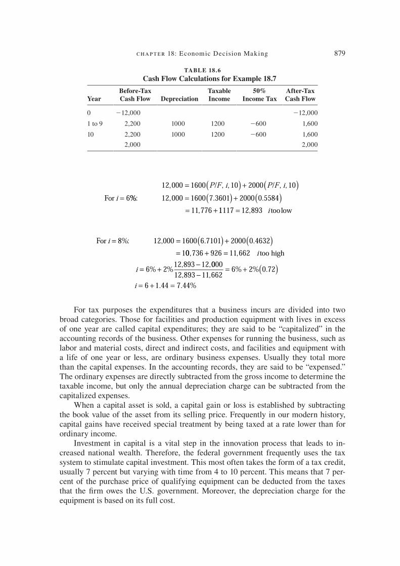
chapter 18: Economic Decision Making 879
12 000 1600 10 2000 10
6
, , , , ,= ( ) + ( )=
P F i P F i
i
/ /
For %% , . .,
: 12 000 1600 7 3601 2000 0 558411 776
= ( ) + ( )= + 11117 12 893= , i toolow
For 8%: 12,000i = = ( ) + ( )=
1600 6 7101 2000 0 46321
. .00 736 926 11 662
6 2 12 893 12, ,
% % , ,+ =
= +−
i
i
too high0000
12 893 11 6626 2 0 72
6 1 44 7 44, ,
% % .
. . %−
= + ( )= + =i
For tax purposes the expenditures that a business incurs are divided into two broad categories. Those for facilities and production equipment with lives in excess of one year are called capital expenditures; they are said to be “capitalized” in the accounting records of the business. Other expenses for running the business, such as labor and material costs, direct and indirect costs, and facilities and equipment with a life of one year or less, are ordinary business expenses. Usually they total more than the capital expenses. In the accounting records, they are said to be “expensed.” The ordinary expenses are directly subtracted from the gross income to determine the taxable income, but only the annual depreciation charge can be subtracted from the capitalized expenses.
When a capital asset is sold, a capital gain or loss is established by subtracting the book value of the asset from its selling price. Frequently in our modern history, capital gains have received special treatment by being taxed at a rate lower than for ordinary income.
Investment in capital is a vital step in the innovation process that leads to in-creased national wealth. Therefore, the federal government frequently uses the tax system to stimulate capital investment. This most often takes the form of a tax credit, usually 7 percent but varying with time from 4 to 10 percent. This means that 7 per-cent of the purchase price of qualifying equipment can be deducted from the taxes that the K rm owes the U.S. government. Moreover, the depreciation charge for the equipment is based on its full cost.
TABLE 18.6
Cash Flow Calculations for Example 18.7
YearBefore-Tax Cash Flow Depreciation
Taxable Income
50% Income Tax
After-Tax Cash Flow
0 212,000 212,000
1 to 9 2,200 1000 1200 2600 1,600
10 2,200 1000 1200 2600 1,600
2,000 2,000
die37039_ch18.indd 879 2/25/08 7:21:39 PM

880 engineering design
18.6 PROFITABILITY OF INVESTMENTS
One of the principal uses for engineering economy is to determine the proK tability of proposed projects or investments. The decision to invest in a project generally is based on three different sets of criteria.
Pro! tability: Determined by techniques of engineering economy to be discussed in this section. ProK tability is an analysis that estimates how rewarding in mon-etary terms an investment will be.
Financial analysis: How to obtain the necessary funds and what it will cost. Funds for investment come from three broad sources: (1) retained earnings of the corporation, (2) long-term commercial borrowing from banks, insurance companies, and pension funds, and (3) the equity market through the sale of stock.
Analysis of intangibles: Legal, political, or social consideration or issues of a corporate image often outweigh K nancial considerations in deciding on which project to pursue. For example, a corporation may decide to invest in the mod-ernization of an old plant because of its responsibility to continue employment for its employees when investment in a new plant 1000 miles away would be economically more attractive.
However, in our free-enterprise system a major goal of a business K rm is to maxi-mize proK t. It does so by committing its funds to ventures that appear to be proK table. If investors do not receive a sufK ciently attractive proK t, they will K nd other uses for their money, and the growth—even the survival—of the K rm will be threatened.
Four methods of evaluating proK tability are commonly used. Accounting rate of return and payback period are simple techniques that are readily understood, but they do not take time value of money into consideration. Net present value and discounted cash Z ow are the most common proK tability measures in which time value of money is considered. Before discussing them, however, we need to look a bit more closely at the concept of cash Z ow.
Cash " ow measures the Z ow of funds into or out of a project. Funds Z owing in constitute positive cash Z ow; funds Z owing out are negative cash Z ow. The cash Z ow for a typical plant construction project is shown in Fig. 18.7. From an accounting point of view, cash Z ow is deK ned as
Cash flow net annual cash income depreciati= + oon
You might consider cash income as “real dollars” and the depreciation an accounting adjustment to allow for capital expenditures. Table 18.7 shows how cash Z ow can be determined in a simple situation.
18.6.1 Rate of Return
The rate of return on the investment (ROI) is the simplest measure of proK tability. It is calculated from a strict accounting point of view without consideration of the time
die37039_ch18.indd 880 2/25/08 7:21:40 PM

chapter 18: Economic Decision Making 881
FIGURE 18.7 Typical costs in the cycle of a plant investment.
Plant start-up
Negative cash flow
Working
capital
Capital
investment
Plant
operation
Payback period
Breakeven
point
Land &
working capital
recovery
Plant
shudown
Time
Total
cumulative
profit
Positive
cash flow
Capital recovery Profitability
Plant
investment
Land
R & D
$–
C
ash
flo
w
$+
0
TABLE 18.7
Calculation of Cash Flow
(1) Revenue (over 1-year period) $500,000
(2) Operating costs 360,000
(3) (1) 2 (2) 5 gross earnings 140,000
(4) Annual depreciation charge 60,000
(5) (3) 2 (4) 5 taxable income 80,000
(6) (5) 3 0.35 5 income tax 28,000
(7) (5) 2 (6) 5 net proK t after taxes 52,000
Net cash Z ow (after taxes) (7) 1 (4) 5 52,000 1 60,000 112,000
die37039_ch18.indd 881 2/25/08 7:21:40 PM

882 engineering design
value of money. It is a simple ratio of some measure of proK t or cash income to the capital investment. There are a number of ways to assess the rate of return on the capi-tal investment. ROI may be based on (1) net annual proK t before taxes, (2) net annual proK t after taxes, (3) annual cash income before taxes, or (4) annual cash income after taxes. These ratios, usually expressed as percents, can be computed for each year or on the average proK t or income over the life of the project. In addition, capital invest-ment sometimes is expressed as the average investment. Thus, although the ROI is a simple concept, it is important in any given situation to understand clearly how it has been determined.
E X A M P L E 1 8 . 8 An initial capital investment is $360,000 and has a 6-year life and a $60,000 salvage value. Working capital is $40,000. Total net proK t after taxes over 6 years is estimated at $167,000. Find the ROI.
Solution
Annual net profit167,000
ROI on in
= =6
28 000$ ,
iitial capital investment28,000
360,000 40,=
+ 0000= 0 07.
18.6.2 Payback Period
The payback period is the period of time necessary for the cash Z ow to fully recover the initial total capital investment (Fig. 18.4). Although the payback method uses cash Z ow, it does not include a consideration of the time value of money. Emphasis is on rapid recovery of the investment. Also, in using the method, no account is taken of cash Z ows or proK ts recovered after the payback period. Consider Table 18.8.
By the payback period criterion, project A is more desirable because it recovers the initial capital investment in 3 years. However, project B, which returns a cumula-tive cash Z ow of $110,000, obviously is more proK table overall.
18.6.3 Net Present Worth
In Sec. 18.3, as one of the techniques of cost comparison, we introduced the criterion of net present worth (NPW).
Net present worth present worth of benefits= −− present worth of costs
By this technique the expected cash Z ows (both 1 and 2) through the life of the proj-ect are discounted to time zero at an interest rate representing the minimum accept-able return on capital, MARR. The project with the greatest positive value of NPW is preferred. NPW depends upon the project life, so strictly speaking the net present worths of two projects should not be compared if the projects have different service lives.
die37039_ch18.indd 882 2/25/08 7:21:40 PM
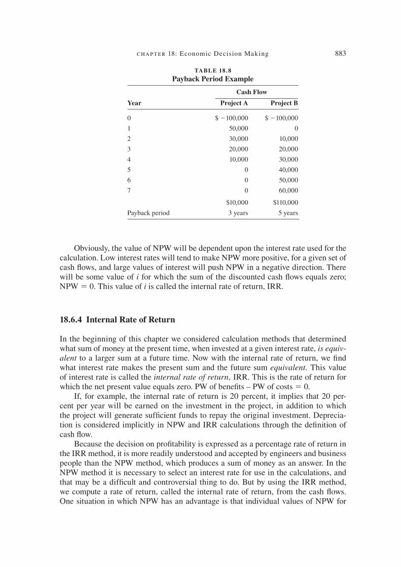
chapter 18: Economic Decision Making 883
Obviously, the value of NPW will be dependent upon the interest rate used for the calculation. Low interest rates will tend to make NPW more positive, for a given set of cash Z ows, and large values of interest will push NPW in a negative direction. There will be some value of i for which the sum of the discounted cash Z ows equals zero; NPW 5 0. This value of i is called the internal rate of return, IRR.
18.6.4 Internal Rate of Return
In the beginning of this chapter we considered calculation methods that determined what sum of money at the present time, when invested at a given interest rate, is equiv-
alent to a larger sum at a future time. Now with the internal rate of return, we K nd what interest rate makes the present sum and the future sum equivalent. This value of interest rate is called the internal rate of return, IRR. This is the rate of return for which the net present value equals zero. PW of beneK ts – PW of costs 5 0.
If, for example, the internal rate of return is 20 percent, it implies that 20 per-cent per year will be earned on the investment in the project, in addition to which the project will generate sufK cient funds to repay the original investment. Deprecia-tion is considered implicitly in NPW and IRR calculations through the deK nition of cash Z ow.
Because the decision on proK tability is expressed as a percentage rate of return in the IRR method, it is more readily understood and accepted by engineers and business people than the NPW method, which produces a sum of money as an answer. In the NPW method it is necessary to select an interest rate for use in the calculations, and that may be a difK cult and controversial thing to do. But by using the IRR method, we compute a rate of return, called the internal rate of return, from the cash Z ows. One situation in which NPW has an advantage is that individual values of NPW for
TABLE 18.8
Payback Period Example
Cash Flow
Year Project A Project B
0 $ 2100,000 $ 2100,000
1 50,000 0
2 30,000 10,000
3 20,000 20,000
4 10,000 30,000
5 0 40,000
6 0 50,000
7 0 60,000
$10,000 $110,000
Payback period 3 years 5 years
die37039_ch18.indd 883 2/25/08 7:21:41 PM

884 engineering design
a series of subprojects may be added to give the NPW for the complete project. That cannot be done with the rate of return developed from IRR analysis.
E X A M P L E 1 8 . 9 A machine has a K rst cost of $10,000 and a salvage value of $2000 after a 5-year life. Annual beneK ts (savings) from its use are $5000, and the annual cost of op-eration is $1800. The tax rate is 50 percent. Find the IRR rate of return.
Solution
Using straight-line depreciation, the annual depreciation charge is
DC C
n
i s=−
=−
=10 000 2 000
51600
, ,$
The annual cash Z ow after taxes is the sum of the net receipts and depreciation.
CFa
( ) = −( ) −( ) + ( )= +
5000 1800 1 0 50 1600 0 50
1600 8
. .
000 2400= $
Year Cash Now
0 210,000
1 2,400
2 2,400
3 2,400
4 2,400
5 2,400 1 2,000 ( C s )
NPW / /= = − + ( ) + ( )0 10 000 2400 5 2000 5, , , , ,P A i P F i
If i 5 10 percent, NPW 5 1340; if i 5 12 percent, NPW 5 2214. Thus, we have the IRR bracketed, and
i = + −( )
+
= +
=
10 12 10340
340 214
10 2340
564
% % %
110 1 2 11 2+ =. . %
The IRR function in Microsoft Excel can be used to quickly determine the internal rate of return. To use IRR, the net beneK ts or costs(-) are entered in a column of cells, one for each period. Enter a 0 for any period where there is no cash Z ow. Finally, enter a guess as the starting point for the calculation. For example: 5IRR(A2:A8,5)
It is an important rule of engineering economy that each increment of investment capital must be justiK ed on the basis of earning the minimum required rate of return.
die37039_ch18.indd 884 2/25/08 7:21:41 PM

chapter 18: Economic Decision Making 885
E X A M P L E 1 8 . 1 0 A company has the option of investing in one of the two machines described in the following table. Which investment is justiK ed?
Machine A Machine B
Initial cost C i $10,000 $15,000
Useful life 5 years 10 years
Salvage value C s $2,000 0
Annual beneK ts $5,000 $7,000
Annual costs $1,800 $4,300
Solution
Assume a 50 percent tax rate and a minimum attractive rate of return of 6 percent. The conditions for machine A are identical with those in Example 18.9, for which i 5 11.2 per-cent. Calculation of the IRR for machine B shows it is slightly in excess of the minimum rate of 6 percent. However, that is not the proper question. Rather, we should ask whether the increment of investment ($15,000 2 $10,000) is justiK ed. In addition, because ma-chine B has twice the useful life of machine A, we should place them both on the same time basis (see Table 18.9).
NPW / /= = − − ( ) + ( ) −0 5000 300 10 8000 5 200P A i P F i, , , , 00 10P F i/ , ,( ) But, even at i = 1
4percent, NPW 5 22009, and there is no way that the extra investment
in machine B can be justiK ed economically.
When only costs—not income (or savings)—are known, we can still use the IRR method for incremental investments, but not for a single project. We assume that the lowest capital investment is justiK ed without being able to determine the internal rate of return, and we then determine whether the additional investment is justiK ed.
TABLE 18.9
Cash Flow, Example 18.10
Year Machine A Machine B Difference, B 2 A
0 210,000 215,000 25,000
1 2,400 2,100 2300
2 2,400 2,100 2300
3 2,400 2,100 2300
4 2,400 2,100 2300
5 2,400 2 10,000 1 2,000 2,100 2300 1 8,000
6 2,400 2,100 2300
7 2,400 2,100 2300
8 2,400 2,100 2300
9 2,400 2,100 2300
10 2,400 1 2,000 2,100 2300 2 2,000
die37039_ch18.indd 885 2/25/08 7:21:41 PM
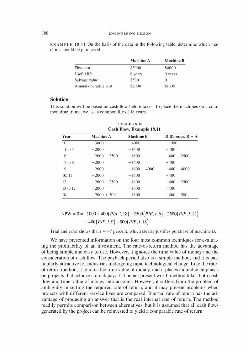
886 engineering design
E X A M P L E 1 8 . 1 1 On the basis of the data in the following table, determine which ma-chine should be purchased.
Machine A Machine B
First cost $3000 $4000
Useful life 6 years 9 years
Salvage value $500 0
Annual operating cost $2000 $1600
Solution
This solution will be based on cash Z ow before taxes. To place the machines on a com-mon time frame, we use a common life of 18 years.
TABLE 18.10
Cash Flow, Example 18.11
Year Machine A Machine B Difference, B A
0 23000 24000 21000
1 to 5 22000 21600 1400
6 22000 2 2500 21600 1400 1 2500
7 to 8 22000 21600 1400
9 22000 21600 2 4000 1400 2 4000
10, 11 22000 21600 1400
12 22000 2 2500 21600 1400 1 2500
13 to 17 22000 21600 1400
18 22000 1 500 21600 1400 2 500
NPW / / ,= = − + ( ) + ( ) +0 1000 400 18 2500 6 250P A i P F i, , , 00 12
400 9 500 18
P F i
P F i P F i
/
/ , /
, ,
, , ,
( )− ( ) − ( )
Trial and error shows that i ø 47 percent, which clearly justiK es purchase of machine B.
We have presented information on the four most common techniques for evaluat-ing the proK tability of an investment. The rate-of-return method has the advantage of being simple and easy to use. However, it ignores the time value of money and the consideration of cash Z ow. The payback period also is a simple method, and it is par-ticularly attractive for industries undergoing rapid technological change. Like the rate-of-return method, it ignores the time value of money, and it places an undue emphasis on projects that achieve a quick payoff. The net present worth method takes both cash Z ow and time value of money into account. However, it suffers from the problem of ambiguity in setting the required rate of return, and it may present problems when projects with different service lives are compared. Internal rate of return has the ad-vantage of producing an answer that is the real internal rate of return. The method readily permits comparison between alternatives, but it is assumed that all cash Z ows generated by the project can be reinvested to yield a comparable rate of return.
die37039_ch18.indd 886 2/25/08 7:21:42 PM

chapter 18: Economic Decision Making 887
18.7 OTHER ASPECTS OF PROFITABILITY
Innumerable factors 5 affect the proK tability of a project in addition to the mathemati-cal expressions discussed in Sec. 18.6. The purpose of this section is to round out our consideration of the crucial subject of proK tability.
We need to realize that proK t and proK tability are not quite the same concept. ProK t is measured by accountants, and its value in any one year can be manipulated in many ways. ProK tability is inherently a long-term parameter of economic decision making. As such, it should not be inZ uenced much by short-term variations in proK ts. In recent years there has been a strong trend toward undue emphasis on quick proK ts and short payoff periods that work to the detriment of long-term investment in high-technology projects.
Estimation of proK tability requires the prediction of future cash Z ows, which in turn requires reliable estimates of sales volume and sales price by the marketing staff and of material price and availability. The quadrupling of crude oil price in 2005 was a dramatic example of how changes in raw material costs can greatly inZ uence proK t-ability predictions. Similarly, trends in operating costs must be looked at carefully, es-pecially with respect to whether it is more proK table to reduce operating costs through increased investment, as with automation.
The estimated investment in machinery and facilities that is required for the proj-ect is usually the most accurate component of the proK tability evaluation. (This topic is considered in more detail in Chap. 16.) The depreciation method used inZ uences how the expense is distributed over the years of a project, and that in turn determines what the cash Z ow will be. However, a more fundamental aspect of depreciation is the effect of writing off a capital investment over a long time period. As a result, costs are underestimated and selling prices are set too low. A long-term write-off combined with inZ ation results in insufK cient cash Z ow to permit reinvestment. InZ ation creates hidden expenses like inadequate allowance for depreciation. When depreciation meth-ods do not allow for inZ ated replacement costs, those costs must be absorbed on an after-tax basis. ProK t and proK tability are overstated in an inZ ationary period.
A number of technical decisions are closely related to the investment policy and proK tability. At the design stage it may be possible to ensure a level of product supe-riority that is more than that needed by the current market. Later, when competitors enter the market, the superiority would prove useful, but it is not achieved without an initial cost to proK tability. Economics generally favor building as large a produc-tion unit as the market can absorb. However, this increased proK tability is achieved at some risk to maintaining continuity of production should the unit be down for repairs. Thus, there often is a trade-off between the increased reliability of having a number of small units over which to spread the risk and a single large unit with somewhat higher proK tability.
The proK tability of a particular product line can be inZ uenced by decisions of cost allocation. Such factors as overhead, utility costs, transfer prices between divisions of a large corporation, or scrap value often require arbitrary decisions for allocation
5. F. C . Jelen , Hydrocarbon Processing, pp. 111–15 , January 1976 .
die37039_ch18.indd 887 2/25/08 7:21:42 PM

888 engineering design
between various products. Thus, the situation often favors certain products and dis-criminates against others because of cost allocation policies. Sometimes corporations take a position of milking an established product line with a limited future (a “cash cow”) in order to stimulate the growth of a new and promising product line. Another proK t decision is whether to charge a particular item as a current expense or capitalize it to make a future expense. In a period of inZ ation there is strong pressure to increase present proK tability by deferring costs into the future by capitalizing them. It is ar-gued that a K xed dollar amount deferred into the future will have less consequence in terms of future dollars.
The role of the government in inZ uencing proK tability is very great. In the broader sense the government creates the general economic climate through its policies on money supply, taxation, and foreign affairs. It provides subsidies to stimulate selected parts of the economy. Its regulatory powers have had an increasing inZ uence on prof-itability in such areas as pollution control, occupational health and safety, consumer protection and product safety, use of federal lands, antitrust, minimum wages, and working hours.
Since proK tability analysis deals with future predictions, there is inevitable un-certainty. Incorporation of uncertainty or risk is possible with advanced techniques. Unfortunately, the assignment of the probability to deal with risk is in itself a subjec-tive decision. Thus, although risk analysis (Sec. 18.10) is an important technique, one should always realize its true origins.
18.8 INFLATION
Since engineering economy deals with decisions based on future Z ows of money, it is important to consider inZ ation in the total analysis. From 1984 to 2006 the average in-Z ation in consumer price has been 4.1 percent. However, there have been years (1974, 1979, and 1980) when the rate of inZ ation was in double digits. 6
InZ ation exists when prices of goods and services are increasing so that a given amount of money buys less and less as time goes by. Interest rates and inZ ation are directly related. The basic interest rate is about 2 to 3 percent higher than the inZ ation rate. Thus, in a period of high inZ ation, not only does the dollar purchase less each month but the cost of borrowing money also rises.
Price changes may or may not be considered in an economic analysis. For mean-ingful results, costs and beneK ts must be computed in comparable units. It would not be sensible to calculate costs in 1990 dollars and beneK ts in 2000 dollars.
InZ ation is measured by the change in the Consumer Price Index (CPI), as de-termined by the U.S. Department of Labor, Bureau of Labor Statistics. 7 The CPI is reported monthly, based on a survey of the price of a “market basket” of goods and services purchased by consumers. In 1984 the CPI was re-centered at 100, and items for price volatile areas such as food and energy were removed, to create the Core CPI.
6 . http://inZ ationdata.com/inZ ation/Consumer_Price_Historical CPI 7 . www.bls.gov/cpi/cpifaq.htm
die37039_ch18.indd 888 2/25/08 7:21:43 PM

chapter 18: Economic Decision Making 889
The CPI in 2007 was 250, compared with 100 in 1984. This means that it would take $250 in 2007 dollars to purchase the same goods and services as in 1984. For design purposes the CPI is less important than the Producer Price Index (PPI), which is dis-cussed in Sec. 16.9.1.
E X A M P L E 1 8 . 1 2 The CPI in 1984 was 100.0, and in 2007 it was 250. 1 Find the rate of inZ ation over this period of 23 years.
F P F P i n F P i F P i= ( ) = ( ) ( ) =/ / /, , . , , , ,250 1 100 23 23 2..501
and on interpolation we K nd f 5 0.041. Another way to K nd the inZ ation rate is to use the equation for annualized return.
Annualized returncurrent value
orginal value=
−
=
= −
1
1
23
1
250 1
100 01 0406 1 00
n
.
.. . 00 0 041 4 1= =. . %
(18.31)
Money in one time period t 1 can be brought to the same value as money in another time period t 2 by the equation
Dollars in periodDollars in period
Int
t1
2=fflation rate between and
1t t
2
(18.32)
It is useful to deK ne two situations: then-current money and constant-value money. Let the dollars in period t 1 be constant-value dollars. Constant-value represents equal purchasing power at any future time. Current money, in time period t 2 , represents ordinary money units that decline in purchasing power with time. For example, if an item cost $10 in 1998 and inZ ation was 3 percent during the previous year, in constant 1997 dollars, the cost is equal to $10/1.03 5 $9.71.
There are three different rates to be considered when dealing with inZ ation.
Ordinary or in" ation-free interest rate i: This is the rate at which interest is earned when effects of inZ ation have been ignored. This is the interest rate we have used up until now in this chapter.
Market interest rate i f : This is the interest rate that is quoted on the business news every day. It is a combination of the real interest rate i and the inZ ation rate f. This is also called the in" ated interest rate.
In" ation rate f: This is a measure of the rate of change in the value of the currency.
Consider the equation for the present worth of a future sum F in current dollars. F must be K rst discounted for the real interest rate and then for the inZ ation rate.
PF
i fF
i f if
F
in n n
f
n
1
1
1
1
1 1+( ) +( )=
+ + +( )=
+( ) (18.33)
where i f 5 i 1 f 1 if is the market interest rate, also called the inZ ated interest rate.
die37039_ch18.indd 889 2/25/08 7:21:43 PM

890 engineering design
E X A M P L E 1 8 . 1 3 A project requires an investment of $10,000 and is expected to return, in future, or “then current,” dollars, $2500 at the end of year 1, $3000 at the end of year 2, and $7000 at the end of year 3. The monetary (ordinary) interest rate is 10 percent, and the inZ ation rate is 6 percent per year. Find the net present worth of this investment opportunity.
Solution
The inZ ated interest rate is 0.10 1 0.06 1 (0.10)(0.06) 5 0.166; for simplicity we shall use i f 5 0.17.
Current-dollars approach
Year Cash Flow ( P / F , 17, n ) Present Worth
0 210,000 1.00 210,000
1 2,500 0.8547 2,137
2 3,000 0.7305 2,191
3 7,000 0.6244 4,971
NPW 5 2711
Constant-Value-Dollars Approach
Year Cash Flow * ( P / F ,10, n ) Present Worth
0 210,000 1.00 210,000
1 2,358 0.9091 2,144
2 2,670 0.8264 2,206
3 5,877 0.7513 4,415
NPW 5 21,235
*Adjusted for f 5 0.06 (1.06)n.
8. F. A . Holland and F. A . Watson , Chem. Eng., pp. 87–91 , Feb. 14, 1977 .
In the current-dollars approach the inZ ated interest rate is used to discount the cash Z ows to the present time. For the constant-dollars approach the cash Z ow is adjusted by [con-stant (real) $] 5 [current (actual) $] (11f)2n.
The difference in the NPWs found by the two treatments is due to using an approxi-mate combined discount rate instead of the more accurate value of i f 5 0.166. However, the approximation is justiK ed in view of the uncertainty in predicting the rate of inZ a-tion. It should be noted that, for this example, the NPW is 1$10 if inZ ation is ignored. That emphasizes the fact that neglecting the inZ uence of inZ ation overemphasizes the proK tability.
When proK tability is measured by the internal rate of return i, the inclusion of the inZ ation rate f results in an effective rate of return i9 based on constant-value money. 8
1 1 1+ = +( ) +( )
= − − −
i i f
i i f i f i f
9
9 9 <
(18.34)
die37039_ch18.indd 890 2/25/08 7:21:43 PM

chapter 18: Economic Decision Making 891
To a K rst approximation, the internal rate of return is reduced by an amount equiva-lent to the average inZ ation rate.
Interest rates are quoted to investors in current money i, but investors generally expect to cover any inZ ationary trends and still receive an acceptable return. In other words, investors hope to obtain a constant-value interest rate i9 . Therefore, the cur-rent interest rate tends to Z uctuate with the inZ ation rate. If the calculation is to be made with constant-value money, discounting should be done with the normal interest rate i. If calculations are in terms of current money, then the discount rate should be i f 5 i 1 f.
Note that tax allowance for depreciation has a reduced beneK t when constant money is used for proK tability evaluations. By law, depreciation is deK ned in terms of current money. Therefore, under high inZ ation when constant-money conditions are appropriate, a full tax credit for depreciation is not achieved.
Another effect of inZ ation is that it increases the cash Z ow because the prices received for goods and services rise as the value of money falls. Even when con-stant-value money is used, the yearly cash Z ows should display the current money situation.
Detailed relations for capitalized cost that include an inZ ation factor have been developed by Jelen. 9 They can also be used to introduce inZ ation calculation into an-nual cost calculations.
18.9 SENSITIVITY AND BREAK-EVEN ANALYSIS
A sensitivity analysis determines the inZ uence of each factor on the K nal result, and therefore it determines which factors are most critical in the economic decision. Since there is a considerable degree of uncertainty in predicting future events like sales volume, salvage value, and rate of inZ ation, it is important to see how much the eco-nomic analysis depends on the magnitude of the estimates. One factor is varied over a reasonable range and the others are held at their mean (expected) value. The amount of computation involved in a sensitivity analysis of an engineering economy problem can be considerable, but the use of computers has made sensitivity analysis a much more practical endeavor.
A break-even analysis often is used when there is particular uncertainty about one of the factors in an economic study. The break-even point is the value for the fac-tor at which the project is just marginally justiK ed.
E X A M P L E 1 8 . 14 Consider a $20,000 investment with a 5-year life. The salvage value is $4000, and the minimal acceptable return is 8 percent. The investment produces an-nual beneK ts of $10,000 at an operating cost of $3000. Suppose there is considerable un-certainty as to whether the new machinery will survive 5 years of continuous use. Find the break-even point, in terms of life, at which the project just becomes economically viable.
9. F. C . Jelen , Chem. Eng., pp. 123–128 , Jan. 27, 1958 .
die37039_ch18.indd 891 2/25/08 7:21:44 PM

892 engineering design
Solution
Using the annual cost method,
$ , , , , .10 000 3000 20 000 4000 8 4000 0 0− − −( )( ) −A P n/ 88 0
86680
16 0000 417
( ) =
( ) = =A P n/ , ,,
.
and interpolating in the interest tables gives us n 5 2.8 years. Thus, if the machine does not last 2.8 years, the investment cannot be justiK ed.
Break-even analysis frequently is used in problems dealing with staged construc-tion. The usual problem is to decide whether to invest more money initially in unused capacity or to add the needed capacity at a later date when needed, but at higher unit costs.
E X A M P L E 1 8 . 14 A new plant will cost $100 million for the K rst stage and $120 million for the second stage at n years in the future. If it is built to full capacity now, it will cost $140 million. All facilities are expected to last 40 years. Salvage value is neglected. Find the preferable course of action.
Solution
The annual cost of operation and maintenance is assumed the same for a two-stage con-struction and full-capacity construction. We shall use a present worth (PW) calculation with a 10 percent interest rate. For full-capacity construction now, PW 5 $140 million ($140M). For two-stage construction
PW $100M $120M /
5 years: PW 00 1
= + ( )= = +
P F n
n
, ,10
1 220 0.6201 M
years: PW 100 120 0.385
( ) =
= = +
$174
10n 55 $146M
20 years: PW 100 120 0.1486
( )=
= = + ( ) =n $1118
30 107
M
years: PW 100 120 0.0573 Mn = = + ( ) = $
These results are plotted in Fig. 18.8. The break-even point (12 years) is the point at which the two alternatives have equivalent cost. If the full capacity will be needed before 12 years, then full capacity built now would be the preferred course of action.
18.10 UNCERTAINTY IN ECONOMIC ANALYSIS
In the preceding sections we discussed the fact that engineering economy deals chieZ y with decisions based on future estimates of costs and beneK ts. Since none of us has a completely clear crystal ball, such estimates are likely to contain considerable un-certainty. In all of the examples presented so far in this chapter we have used a single value that was the implied best estimate of the future.
die37039_ch18.indd 892 2/25/08 7:21:44 PM
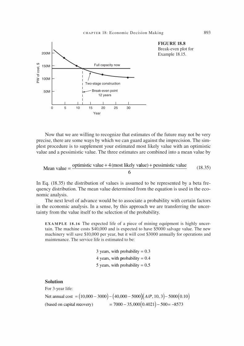
chapter 18: Economic Decision Making 893
Now that we are willing to recognize that estimates of the future may not be very precise, there are some ways by which we can guard against the imprecision. The sim-plest procedure is to supplement your estimated most likely value with an optimistic value and a pessimistic value. The three estimates are combined into a mean value by
Mean valueoptimistic value 4 (most likely v
=+ aalue) pessimistic value+
6 (18.35)
In Eq. (18.35) the distribution of values is assumed to be represented by a beta fre-quency distribution. The mean value determined from the equation is used in the eco-nomic analysis.
The next level of advance would be to associate a probability with certain factors in the economic analysis. In a sense, by this approach we are transferring the uncer-tainty from the value itself to the selection of the probability.
E X A M P L E 1 8 . 1 6 The expected life of a piece of mining equipment is highly uncer-tain. The machine costs $40,000 and is expected to have $5000 salvage value. The new machinery will save $10,000 per year, but it will cost $3000 annually for operations and maintenance. The service life is estimated to be:
3 years, with probability 0.3
4 years, with
=pprobability 0.4
5 years, with probability 0
== ..5
Solution
For 3-year life:
Net annual cost 10,000 3000 40,000 5000= −( ) − −( ))( )− ( )A P/
based on capital re
, , .
(
10 3 5000 0 10
ccovery) , .= − ( ) − = −7000 35 000 0 4021 500 8573
FIGURE 18.8 Break-even plot for Example 18.15.
Full capacity now
PW
of
co
st,
$
50
50M
10 15 20
Year
Break-even point
12 years
Two-stage construction
25 30
100M
150M
200M
die37039_ch18.indd 893 2/25/08 7:21:45 PM

894 engineering design
For 4-year life:
Net annual cost 7000= − 35 000, 00 3155 500 4542.( ) − = −
For 5-year life:
Net annuual cost 7000
Expe
= − ( ) − = −35 000 0 2638 500 2733, .
ccted value of net annual cost AC AC A= ( ) = ∑ ×E P CC( ) =
− ( ) + − ( ) + − ( )8573 0 3 4542 0 4 2733 0 3. . . = −5207
18.11 BENEFIT-COST ANALYSIS
An important class of engineering decisions involves the selection of the preferred system design, material, purchased subsystem, etc., when economic resources are constrained. The methods of making cost comparisons and proK tability analysis de-scribed in Secs. 18.3 and 18.6 are important decision-making tools in this type of situation.
Frequently, comparisons are based on a bene! t-cost ratio, which relates the de-sired beneK ts to the capital investment required to produce the beneK ts. This method of selecting alternatives is most commonly used by governmental agencies for deter-mining the desirability of public works projects. A project is considered viable when the net beneK ts associated with its implementation exceed its associated costs. Bene! ts are advantages to the public (or owner), expressed in terms of dollars. If the project in-volves disadvantages to the owner, these disbene! ts must be subtracted from the ben-eK ts. The costs to be considered include the expenditures for construction, operation, and maintenance, less salvage. Both beneK ts, disbeneK ts, and costs must be expressed in common monetary terms by using the present worth or annual cost concept.
Benefit-cost ratio BCRbenefits disbenefi( ) =
− tts
costs (18.36)
A design or project for which BCR < 1 does not cover the cost of capital to create the design. Generally, only projects for which BCR > 1 are acceptable. The beneK ts used in the BCR would be factors like improved component performance, increased payload through reduced weight, and increased availability of equipment. BeneK ts are deK ned as the advantages minus any disadvantages, that is, the net beneK ts. Likewise, the costs are the total costs minus any savings. The costs should represent the initial capital cost as well as costs of operation and maintenance; see Chap. 16.
In problems of choosing between several alternatives, the incremental or marginal beneK ts and costs associated with changes beyond a base level or reference design should be used. The alternatives are ranked with respect to cost, and the lowest-cost situation is taken as the initial reference. This is compared with the next higher-cost alternative by computing the incremental beneK t and incremental cost. If ∆ B /∆ C < 1, then alternative 2 is rejected because the K rst alternative is superior. Alternative 1 now is compared with alternative 3. If ∆ B /∆ C > 1, then alternative 1 is rejected and
die37039_ch18.indd 894 2/25/08 7:21:45 PM

chapter 18: Economic Decision Making 895
alternative 3 becomes the current best solution. Alternative 3 is compared with num-ber 4, and if ∆ B /∆ C < 1, then alternative 3 is the best choice. We should note that this may not be the alternative with the largest overall beneK t-cost ratio.
E X A M P L E 1 8 . 17 You are asked to recommend a site for a small dam to generate hydro-electric power. The construction cost at various sites is given in the following table. These vary with topography and soil conditions. Each estimate includes $3M for the turbines and generators. The annual beneK ts from the sale of electricity vary between sites be-cause of stream velocity.
We require an annual return of 10 percent. The life of the dam is inK nite for purposes of calculation. The hydroelectric machinery has a 40-year life.
SiteConstruction
Cost, $MCost of
Machinery, $MCost of
Dam, $MAnnual
Income, $M
A 9 3 6 1.0
B 8 3 5 0.9
C 12 3 9 1.25
D 6 3 3 0.5
Since the beneK t (income) is on an annual basis, we have to convert the cost to an annual basis. Also, we are going to make our decision on an incremental basis. We construct Table 18.11, placing the alternatives in order of increasing cost (from left to right).
For example, the annual cost of capital recovery for A 5 P D i 1 P H-E ( A/p , 10, 40)
Annual costof capital recovery 6,000,000 0.10= ( ) ++ ( )
= + =
3 000 000 0 1023
600 000 306 900 907 00
, , .
, , $ , 00
We note that when compared to not building a dam, ∆B/∆C for site D is less than 1.0. The next-lowest-cost dam site is greater than 1.0, so it is selected in comparison to not building a dam. The beneK t-cost ratio for sites A and C also is greater than 1.0, but now,
TABLE 18.11
Site Benea t-Cost Analysis, Example 18.17
D B A C
Annual cost of capital recovery ($1000)
607 807 907 1207
Annual beneK ts ($1000)
500 900 1000 1250
Comparison D to do nothing
B to do nothing
A to B C to B
∆ capital recovery 607 807 100 400
∆ annual beneK ts 500 900 100 350
∆B/∆C 0.82 1.11 1.00 0.87
Selection Do nothing B B B
die37039_ch18.indd 895 2/25/08 7:21:45 PM

896 engineering design
having found a low-cost qualifying site (B), we need to determine whether the increment in beneK ts and costs is better than B. We see that on a ∆B/∆C basis, A and C are not better choices than B. Therefore, we select site B.
When used in a strictly engineering context to aid in the selection of alternative materials, the beneK t-cost ratio is a useful decision-making tool. However, it often is used with regard to public projects K nanced with tax monies and intended to serve the overall public good. There is a psychological advantage to the BCR concept over the internal rate of return in that it avoids the connotation that the government is proK ting from public monies. Here questions that go beyond economic efK ciency become part of the decision process. Many of the broader issues are difK cult to quantify in mon-etary terms. Of even greater difK culty is the problem of relating monetary cost to the real values of society.
Consider the case of a hydroelectric facility. The dam produces electricity, but it also will provide Z ood control and an area for recreational boating. The value of each of the outputs should be included in the beneK ts. The costs include the expenditures for construction, operation, and maintenance. However, there may be social costs like the loss of virgin timberland or a scenic vista. Great controversy surrounds the assign-ment of costs to environmental and aesthetic issues.
Although beneK t-cost analysis is a widely used methodology, it is not without problems. The assumption is that costs and beneK ts are relatively independent. Basi-cally, it is a deterministic method that does not deal with uncertainty in a major way. As with most techniques, it is best not to try to push it too far. Although the quantita-tive ratios provided by Eq. (18.36) should be used to the greatest extent possible, they should not preempt the utilization of common sense and good judgment.
18.12 SUMMARY
Engineering economy is the methodology that promotes rational decision making about the allocation of amounts of money at various points in time and in various manners—for example, as a uniform series over time or a single payment in the fu-ture. As such, engineering economy accounts for the time value of money.
The basic relationship is the compound interest formula that relates the future sum F to the present sum P over n years at an interest rate i .
F P in
= +( )1
If P is solved for in this equation, we are discounting the future sum F back to the present time. If the money occurs as equal end-of-the-period amounts A , then
F Ai
i
n
=+( ) −1 1
If this equation is solved for A , it gives the annual payment to provide a sinking fund to replace worn-out equipment. More important is the annual payment to return
die37039_ch18.indd 896 2/25/08 7:21:46 PM
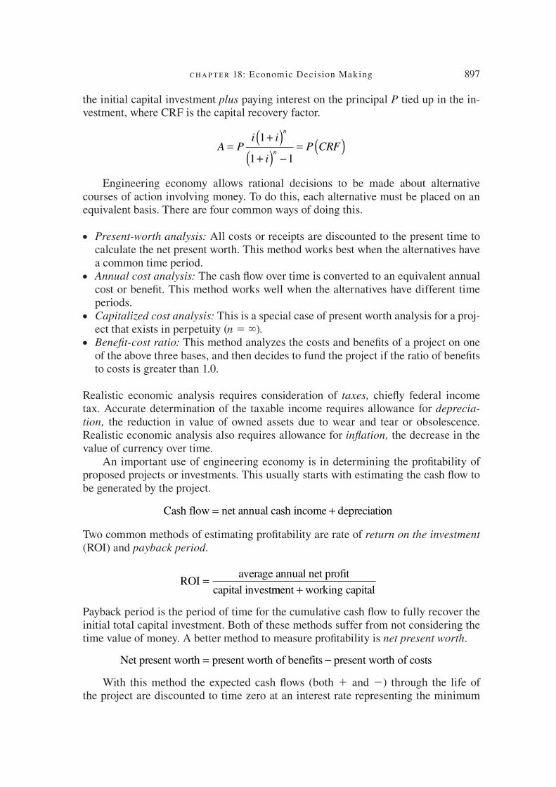
chapter 18: Economic Decision Making 897
the initial capital investment plus paying interest on the principal P tied up in the in-vestment, where CRF is the capital recovery factor.
A Pi i
iP CRF
n
n=
+( )+( ) −
= ( )1
1 1
Engineering economy allows rational decisions to be made about alternative courses of action involving money. To do this, each alternative must be placed on an equivalent basis. There are four common ways of doing this.
Present-worth analysis: All costs or receipts are discounted to the present time to calculate the net present worth. This method works best when the alternatives have a common time period.
Annual cost analysis: The cash Z ow over time is converted to an equivalent annual cost or beneK t. This method works well when the alternatives have different time periods.
Capitalized cost analysis: This is a special case of present worth analysis for a proj-ect that exists in perpetuity ( n 5 `).
Bene! t-cost ratio: This method analyzes the costs and beneK ts of a project on one of the above three bases, and then decides to fund the project if the ratio of beneK ts to costs is greater than 1.0.
Realistic economic analysis requires consideration of taxes, chieZ y federal income tax. Accurate determination of the taxable income requires allowance for deprecia-
tion, the reduction in value of owned assets due to wear and tear or obsolescence. Realistic economic analysis also requires allowance for in" ation, the decrease in the value of currency over time.
An important use of engineering economy is in determining the proK tability of proposed projects or investments. This usually starts with estimating the cash Z ow to be generated by the project.
Cash flow net annual cash income depreciati= + oon
Two common methods of estimating proK tability are rate of return on the investment
(ROI) and payback period.
ROIaverage annual net profit
capital invest=
mment working capital+
Payback period is the period of time for the cumulative cash Z ow to fully recover the initial total capital investment. Both of these methods suffer from not considering the time value of money. A better method to measure proK tability is net present worth.
Net present worth present worth of benefits= −− present worth of costs
With this method the expected cash Z ows (both 1 and 2) through the life of the project are discounted to time zero at an interest rate representing the minimum
●
●
●
●
die37039_ch18.indd 897 2/25/08 7:21:46 PM

898 engineering design
acceptable return on capital. The internal rate of return (IRR) is the interest rate for which the net present worth equals zero.
Net PW PW benefits PW costs= ( ) − ( ) = 0
Since there is considerable uncertainty in estimating future income streams and costs, engineering economic studies often estimate a range of values and utilize a mean value. Another approach is to place probabilities on the values and use an ex-pected value in the analysis.
NEW TERMS AND CONCEPTS
Annual cost analysis BeneK t-cost analysis Capitalized cost Capital recovery factor Cash Z ow Current dollars Declining balance depreciation Depreciation
Discounting to the present Effective interest rate Future value InZ ation rate Internal rate of return MACRS Marginal incremental return MARR
Net present worth Nominal interest rate Payback period Present value Present worth analysis Sinking fund factor Time value of monety Uniform annual series
BIBLIOGRAPHY
Blank , L. T ., and A. J . Tarquin : Engineering Economy, 6th ed., McGraw-Hill, New York , 2004 .
Canada , J. R .: Intermediate Economic Analysis for Management and Engineering, Prentice Hall, Englewood Cliffs, NJ , 1971 .
Humphreys , K. K .: Jelen’s Cost and Optimization Engineering, 3d ed., McGraw-Hill, New York , 1990 .
Newnan , D. G ., and J. P . Lavelle : Engineering Economics Analysis, 7th ed., Engineering Press, San Jose, CA , 1998 .
Park , C. S .: Contemporary Engineering Economics, 2d ed., Addison-Wesley, Reading, MA , 1996 .
Thuesen , G. J ., and W. J . Fabrycky : Engineering Economy, 8th ed., Prentice Hall, Englewood Cliffs, NJ , 1993 .
White , J. A ., K. E . Case , D. B . Pratt , and M. H . Agee , Principles of Engineering Economic
Analysis, 4th ed., John Wiley & Sons, New York , 1997 .
PROBLEMS AND EXERCISES
The interest tables at the end of this chapter are available to help you solve these problems. Also, note that computer spreadsheet software provides most of the X nancial functions dis-cussed in this chapter. It is recommended that you use a spreadsheet to solve the problems.
die37039_ch18.indd 898 2/25/08 7:21:46 PM

chapter 18: Economic Decision Making 899
18.1. (a) Calculate the amount realized at the end of 7 years through annual deposits of $1000 at 10 percent compound interest.
(b) What would the amount be if interest were compounded semiannually?
18.2. A young woman purchases a new car. After down payment and allowances, the amount to be paid is $8000. If money is available at 10 percent, what is the monthly payment to pay off the loan in 4 years? What would it be at 4 percent interest?
18.3. A new machine tool costs $15,000 and has a $5000 salvage value at the end of 5 years. The interest rate is 10 percent. The annual cost of capital recovery is the annual depre-ciation charge (use straight-line depreciation) plus the equivalent annual interest charge. Work this out on a year-by-year basis and show that it equals the number obtained quickly by using the capital recovery factor.
18.4. A father desires to establish a fund for his new child’s college education. He estimates that the current cost of a year of college education is $12,000 and that the cost will esca-late at an annual rate of 4 percent. (a) What amount is needed on the child’s eighteenth, nineteenth, twentieth, and
twenty-X rst birthdays to provide for a 4-year college education? (b) If a rich aunt gives $5000 on the day the child is born, how much must be set aside
at 10 percent on each of the X rst through seventeenth birthdays to build up the col-lege fund?
18.5. A major industrialized nation manages its X nances in such a way that it runs an annual trade deX cit with other countries of $100 billion. If the cost of borrowing is 10 percent, how long will it be before the debt (accumulated deX cit) is one trillion dollars ($1000B)? If nothing is done, how long will it take to accumulate the second $1000B debt?
18.6. Machine A costs $8500 and has annual operating costs of $4500. Machine B costs $7000 and has an annual operating cost of $4800. Each machine has an economic life of 10 years. If the minimum required rate of return is 10 percent, compare the advan-tages of machine A by (a) present worth method, (b) annual cost method, and (c) rate of return on investment.
18.7. Make a cost comparison between two conveyor systems for transporting raw materials.
System A System B
Installed cost $25,000 $15,000
Annual operating cost 6,000 11,000
The service life of each system is 5 years and the write-off period is 5 years. Use straight-line depreciation and assume no salvage value for either system. At what rate of return after taxes would B be more attractive than A?
18.8. A resurfaced k oor costs $5000 and will last 2 years. If money is worth 10 percent after taxes, how long must a new k oor costing $19,000 last to be economically justiX ed? The tax rate is 52 percent. For tax purposes a new k oor can be written off in 1 year. Use sum-of-the-years-digits depreciation. Use the capitalized cost method for your analysis.
die37039_ch18.indd 899 2/25/08 7:21:46 PM

900 engineering design
18.9. You are concerned with the purchase of a heat-treating furnace for the gas carburizing of steel parts. Furnace A will cost $325,000 and will last 10 years; furnace B will cost $400,000 and will also last 10 years. However, furnace B will provide closer control on case depth, which means that the heat treater can shoot for the low side of the speciX cation range on case depth. That will mean that the production rate for furnace B will be 2740 lb/h compared with 2300 lb/h for furnace A. Total yearly production is required to be 15,400,000 lb. The cycle time for furnace A is 16.5 h, and that for fur-nace B is 13.8 h. The hourly operating cost is $64.50 per h.
Justify the purchase of furnace B on the basis of (a) payout time and (b) discounted cash k ow rate of return after taxes. (c) Assume money is worth 10 percent and the tax rate is 50 percent.
18.10. The cost of capital has a strong ink uence on the willingness of management to in-vest in long-term projects. If the cost of capital in America is 10 percent and in Japan 4 percent, what must the return be after 2 years on a 2-year investment of $1 million for each of the situations to provide an acceptable return on the investment? Repeat the analysis for a 20-year period.
18.11. In order to justify investment in a new plating facility, it is necessary to determine the present worth of the costs.
Calculate the present worth given the following information:
Cost of equipment $350,000 Planning period 5 years Fixed charges 20 percent of investment each year Variable charges 40,000 X rst year, escalating at 6 percent each year with
ink ation starting at t 5 0 Rate of return i 5 10%
18.12. Determine the net present worth of the costs for a major construction project under the following set of conditions: (a) Estimated cost $300 million over 3 years (baseline case). (b) Project is delayed by 3 years with rate of ink ation 10 percent and interest cost 16
percent. (c) Project is delayed 6 years with rate of ink ation 10 percent and interest costs 16
percent.
18.13. Whether a maintenance operation is classiX ed as a repair (expense charged against revenues in current year) or improvement (capitalized expense) can have a big ink u-ence on taxes. Determine the net savings for a $10,000 operation using the two differ-ent approaches if (a) you are in a business that is in the 50 percent tax bracket and (b) you are in a small business in the 20 percent tax bracket. Use a 10 percent interest rate and a 10 percent investment tax credit.
18.14. As a new professional employee you need to worry about your retirement many years in the future. Construct a table showing how much you need to have invested, at 4 per-cent, 8 percent, and 12 percent annual rate of return, to provide each $100 of monthly income. Assume that ink ation will increase at 3 percent annually, so the numbers you
die37039_ch18.indd 900 2/25/08 7:21:47 PM

chapter 18: Economic Decision Making 901
calculate will be in ink ation-adjusted dollars. Calculate the monthly amount needed for a retirement period of 25, 30, 35, and 40 years. Assume that the investments are made in tax-sheltered accounts.
18.15. At what annual mileage is it cheaper to provide your X eld representatives with cars than to pay them $0.32 per mile for the use of their own cars? The costs of furnishing a car are as follows:
Purchase price $9000 Life 4 years Salvage $1500 Storage $150 per year Maintenance $0.08 per mile (a) Assume i 5 10 percent. (b) Assume i 5 16 percent.
18.16. To levelize expenditures means to create a uniform end-of-year payment that will have the same present worth as a series of irregular end-of-year payments. To illustrate, consider the estimated 5-year maintenance budget for a pilot plant. Develop a levelized cost assuming that i 5 0.10 and the annual ink ation escalation will be 8 percent.
Year
Maintenance
Budget Estimate
1 25,000
2 150,000
3 60,000
4 70,000
5 300,000
18.17. The marketing department made the following estimates about four different product designs. Use beneX t-cost analysis to determine which design to pursue.
Design
Unit
Manufacturing Cost Sales Price
Est.
Annual Sales
A 12.50 25.00 250,00
B 22.00 40.00 200,00
C 15.00 25.00 250,00
D 15.00 20.00 300,00
18.18. You buy 100 shares of stock in QBC Corp. at $40 per share. It is a good buy, for 4 years, 3 months later you sell these shares of stock for $114 7/8. What is the annual rate of return on this fortunate investment?
die37039_ch18.indd 901 2/25/08 7:21:47 PM

AA
A-1
Appendix A
STATISTICS
This appendix provides a brief overview of the use of statistics in engineering prac-tice. Probability and statistics are working tools of engineers. Prediction of behavior from the past data of well-understood processes is a critical step in many tasks of the design process. Just as important in engineering design is the analysis of data from sample test results and other predictions of behavior of new and less-understood de-signs. Engineering training includes some degree of study in the mathematical disci-plines of probability and statistics.
Probability is the study of a known population of data to predict the characteristics of a single observation from a population or set of observations taken from the popula-tion in a meaningful way. For example, Sec. 8.6 introduces the standard normal distri-bution to describe concepts of statistical tolerancing, and Appendix B holds the proba-bility tables for the z distribution. The Weibull distribution is used in Sec. 13.3 in regard to reliability theory. Engineers will use the principles of probability to create simula-tion models of events that occur with a known probability distribution as in Sec. 10.7.
Engineering practice also requires the use of statistical analysis. Statistics is the study of a sample of observations from a population to make inferences about the en-tire population. Statistical analysis is used to create the control charts for monitoring process accuracy (Secs 14.4 and 14.5). An engineer will take samples of observations from a batch of manufactured parts for measurement in order to infer key characteris-tics of the entire batch of parts.
A.1 BASIC DESCRIPTIVE CHARACTERISTICS
FOR A POPULATION AND A SAMPLE
There are two different types of data sets that an engineer will encounter in practice: a population and a sample. Formulas for basic descriptive statistics are listed Table A.1. The average values are calculated the same for all data sets, but the variance is not.
die37039_ch17_apa.indd A-1 2/25/08 7:03:57 PM
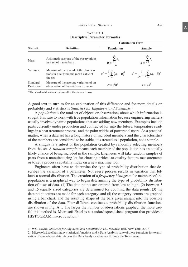
appendix a: Stat ist ics A-2A
A good text to turn to for an explanation of this difference and for more details on probability and statistics is Statistics for Engineers and Scientists . 1
A population is the total set of objects or observations about which information is sought. It is rare to work with true population information because engineering matters usually involve dynamic populations that are adding new members. Examples include parts currently under production and contracted for into the future, temperature read-ings in a heat treatment process, and the palm widths of power tool users. As a practical matter, when a data set has a long history of included members and the characteristics of the members are considered to be stable, it is treated as a population, not a sample.
A sample is a subset of the population created by randomly selecting members from the set. A random sample means each member of the population has an equally likely chance of being included in the sample. Engineers will take random samples of parts from a manufacturing lot for charting critical-to-quality feature measurements or to set a process capability index on a new machine tool.
Engineers often have to determine the type of probability distribution that de-scribes the variation of a parameter. Not every process results in variation that fol-lows a normal distribution. The creation of a frequency histogram for members of the population is a graphical way to begin determining the type of probability distribu-tion of a set of data. (1) The data points are ordered from low to high; (2) between 5 and 15 equally sized categories are determined for counting the data points; (3) the data point counts are made for each category; and (4) the category counts are graphed using a bar chart, and the resulting shape of the bars gives insight into the possible distribution of the data. Four different continuous probability distribution functions are shown in Fig. A.1. The larger the number of observations graphed, the more use-ful this method is. Microsoft Excel is a standard spreadsheet program that provides a HISTOGRAM macro function. 2
TABLE A.1
Descriptive Parameter Formulas
Calculation Form
Statistic De7 nition Population Sample
MeanArithmetic average of the observations
in a set of n members.
µ = =
∑ x
n
ii
n
1
x
x
n
ii
n
= =
∑1
Variance Measure of the spread of the observa-
tions in a set from the mean value of
the set σ µ2 2
1
1= −( )
=
∑n
xi
i
n
s
nx x
ii
n2 2
1
1
1=
−−
=
∑( )
( )
Standard
Deviation *
Measure of the average variation of an
observation of the set from its mean σ σ= 2
s s= 2
* The standard deviation is also called the standard error.
1. W.C. Navidi, Statistics for Engineers and Scientists, 2d ed., McGraw-Hill, New York, 2007.
2. Microsoft Excel has many statistical functions and a Data Analysis suite of these functions for exami-
nation of spreadsheet data. Access the Data Analysis submenu through the Tools menu.
die37039_ch17_apa.indd A-2 2/25/08 7:03:58 PM

A-3 engineering design A
Histograms appear in several sections of the text. Example 10.6 includes a set of histo-grams for the length of three separate parts and their resulting assembly.
A.2 SAMPLING DISTRIBUTION
An engineer will take multiple random samples of data from the same population to determine its statistical parameters. Each sample must be of the same size, n . Each sample will have its own mean, called the sample mean (indicated by x
_ or X
_ ) which
will vary between the samples. The means of all the samples of size n make up a new probability distribution called the sampling distribution . If the underlying population has a normal distribution with a mean of m and a standard deviation of s (the values exist but are not known), the sampling distribution will also have a normal distribu-tion with the same mean of m and a standard deviation as follows:
σσ
xn
= (A.1)
Often an engineer must make inferences about a population using only small sam-ples from that population. This occurs when creating control charts for a dimension on a new part or when determining if feature dimensions comply with specij cations. In these situations, the engineer will take samples and create a sampling distribution to estimate the mean and standard deviation of the entire population. This is easily done if the original population is known to follow a normal distribution. When you cannot make the assumption that a population is normally distributed, you use the results of the Central Limit Theorem.
Engineers need to use statistics from sampling distributions to estimate the value of the mean of the population. A conj dence interval for the actual mean when s is known is given by Eq. (A.2) using the z statistic and values from z tables.
x zn
x zn
− < < +α α
σµ
σ
2 2
. (A.2)
If s of the population is not known, you must use the t statistic (Sec A.4) instead of the z statistic.
FIGURE A.1
Shapes of different probability distribution functions.
Exponential
1
0.0 0.4
0.4
0.3
0.2
0.10.10.2 2
2
1
0.1
0.2
0.3
0.4
0.5
1.00
Normal Uniform Beta
( 5 1, 5 1, 5 1)l ! ( 5 1, 5 2, 5 0.714)a b ( 5 1, 5 1) ! ( 5 1, 5 0.577) !
die37039_ch17_apa.indd A-3 2/25/08 7:03:58 PM
appendix a: Stat ist ics A-4A
A.3 THE CENTRAL LIMIT THEOREM
The Central Limit Theorem applies to any population having a mean of μ and a stan-dard deviation of s (the values exist but the engineer does not know them), regardless of its probability distribution. The variable x
_ is the sample mean of a single sample n
of independent observations randomly chosen from the total population. The Central Limit Theorem states that the sampling distribution for x
_ (i.e., the distribution of the
sample mean values) will be a normal distribution with mean of m and a standard de-viation given in Eq. (A.1) when n is large (about 30 observations or more). This result also holds for samples of a size less than 30 if the original distribution is symmetric.
A.4 THE T DISTRIBUTION
Engineers usually need to estimate mean and standard deviation values for unknown populations in a quick and reliable fashion. The Central Limit Theorem will not apply if nothing is known about the population and only small samples ( n , 30) are avail-able. When the engineer can assume that the population is approximately normal, the distribution of a test statistic given by Eq. (A.3) will follow the t distribution (also called the Student’s t distribution).
X
sn
n−
−( )µ, with degrees of freedom.1 (A.3)
The t distribution is shaped like a standard normal distribution but is wider with a lower maximum and thicker tails. As the degrees of freedom of the t distribution increase toward 30, s approaches s and the t distribution curve approaches the z curve. Values for the probabilities of points along the t curve are compiled in t tables (Appendix C).
die37039_ch17_apa.indd A-4 2/25/08 7:03:59 PM

B
B-1
Appendix B
AREA UNDER THE CUMULATIVE DISTRIBUTION FUNCTION FOR Z
die37039_ch18_apb.indd B-1 2/25/08 7:05:09 PM

appendix b: Area Under the Cumulat ive Dist r ibution Function for z B-2
B
z 0.00 0.01 0.02 0.03 0.04 0.05 0.06 0.07 0.08 0.09
23.6 .0002 .0002 .0001 .0001 .0001 .0001 .0001 .0001 .0001 .0001
23.5 .0002 .0002 .0002 .0002 .0002 .0002 .0002 .0002 .0002 .0002
23.4 .0003 .0003 .0003 .0003 .0003 .0003 .0003 .0003 .0003 .0002
23.3 .0005 .0005 .0005 .0004 .0004 .0004 .0004 .0004 .0004 .0003
23.2 .0007 .0007 .0006 .0006 .0006 .0006 .0006 .0005 .0005 .0005
23.1 .0010 .0009 .0009 .0009 .0008 .0008 .0008 .0008 .0007 .0007
23.0 .0013 .0013 .0013 .0012 .0012 .0011 .0011 .0011 .0010 .0010
22.9 .0019 .0018 .0018 .0017 .0016 .0016 .0015 .0015 .0014 .0014
22.8 .0026 .0025 .0024 .0023 .0023 .0022 .0021 .0021 .0020 .0019
22.7 .0035 .0034 .0033 .0032 .0031 .0030 .0029 .0028 .0027 .0026
22.6 .0047 .0045 .0044 .0043 .0041 .0040 .0039 .0038 .0037 .0036
22.5 .0062 .0060 .0059 .0057 .0055 .0054 .0052 .0051 .0049 .0048
22.4 .0082 .0080 .0078 .0075 .0073 .0071 .0069 .0068 .0066 .0064
22.3 .0107 .0104 .0102 .0099 .0096 .0094 .0091 .0089 .0087 .0084
22.2 .0139 .0136 .0132 .0129 .0125 .0122 .0119 .0116 .0113 .0110
22.1 .0179 .0174 .0170 .0166 .0162 .0158 .0154 .0150 .0146 .0143
22.0 .0228 .0222 .0217 .0212 .0207 .0202 .0197 .0192 .0188 .0183
21.9 .0287 .0281 .0274 .0268 .0262 .0256 .0250 .0244 .0239 .0233
21.8 .0359 .0351 .0344 .0336 .0329 .0322 .0314 .0307 .0301 .0294
21.7 .0446 .0436 .0427 .0418 .0409 .0401 .0392 .0384 .0375 .0367
21.6 .0548 .0537 .0526 .0516 .0505 .0495 .0485 .0475 .0465 .0455
21.5 .0668 .0655 .0643 .0630 .0618 .0606 .0594 .0582 .0571 .0559
21.4 .0808 .0793 .0778 .0764 .0749 .0735 .0721 .0708 .0694 .0681
21.3 .0968 .0951 .0934 .0918 .0901 .0885 .0869 .0853 .0838 .0823
21.2 .1151 .1131 .1112 .1093 .1075 .1056 .1038 .1020 .1003 .0985
21.1 .1357 .1335 .1314 .1292 .1271 .1251 .1230 .1210 .1190 .1170
21.0 .1587 .1562 .1539 .1515 .1492 .1469 .1446 .1423 .1401 .1379
20.9 .1841 .1814 .1788 .1762 .1736 .1711 .1685 .1660 .1635 .1611
20.8 .2119 .2090 .2061 .2033 .2005 .1977 .1949 .1922 .1894 .1867
20.7 .2420 .2389 .2358 .2327 .2296 .2266 .2236 .2206 .2177 .2148
20.6 .2743 .2709 .2676 .2643 .2611 .2578 .2546 .2514 .2483 .2451
20.5 .3085 .3050 .3015 .2981 .2946 .2912 .2877 .2843 .2810 .2776
20.4 .3446 .3409 .3372 .3336 .3300 .3264 .3228 .3192 .3156 .3121
20.3 .3821 .3783 .3745 .3707 .3669 .3632 .3594 .3557 .3520 .3483
20.2 .4207 .4168 .4129 .4090 .4052 .4013 .3974 .3936 .3897 .3859
20.1 .4602 .4562 .4522 .4483 .4443 .4404 .4364 .4325 .4286 .4247
20.0 .5000 .4960 .4920 .4880 .4840 .4801 .4761 .4721 .4681 .4641
0z
die37039_ch18_apb.indd B-2 2/25/08 7:05:10 PM

B-3 engineering design
B
0 z
z 0.00 0.01 0.02 0.03 0.04 0.05 0.06 0.07 0.08 0.09
0.0 .5000 .5040 .5080 .5120 .5160 .5199 .5239 .5279 .5319 .5359
0.1 .5398 .5438 .5478 .5517 .5557 .5596 .5636 .5675 .5714 .5753
0.2 .5793 .5832 .5871 .5910 .5948 .5987 .6026 .6064 .6103 .6141
0.3 .6179 .6217 .6255 .6293 .6331 .6368 .6406 .6443 .6480 .6517
0.4 .6554 .6591 .6628 .6664 .6700 .6736 .6772 .6808 .6844 .6879
0.5 .6915 .6950 .6985 .7019 .7054 .7088 .7123 .7157 .7190 .7224
0.6 .7257 .7291 .7324 .7357 .7389 .7422 .7454 .7486 .7517 .7549
0.7 .7580 .7611 .7642 .7673 .7704 .7734 .7764 .7794 .7823 .7852
0.8 .7881 .7910 .7939 .7967 .7995 .8023 .8051 .8078 .8106 .8133
0.9 .8159 .8186 .8212 .8238 .8264 .8289 .8315 .8340 .8365 .8389
1.0 .8413 .8438 .8461 .8485 .8508 .8531 .8554 .8577 .8599 .8621
1.1 .8643 .8665 .8686 .8708 .8729 .8749 .8770 .8790 .8810 .8830
1.2 .8849 .8869 .8888 .8907 .8925 .8944 .8962 .8980 .8997 .9015
1.3 .9032 .9049 .9066 .9082 .9099 .9115 .9131 .9147 .9162 .9177
1.4 .9192 .9207 .9222 .9236 .9251 .9265 .9279 .9292 .9306 .9319
1.5 .9332 .9345 .9357 .9370 .9382 .9394 .9406 .9418 .9429 .9441
1.6 .9452 .9463 .9474 .9484 .9495 .9505 .9515 .9525 .9535 .9545
1.7 .9554 .9564 .9573 .9582 .9591 .9599 .9608 .9616 .9625 .9633
1.8 .9641 .9649 .9656 .9664 .9671 .9678 .9686 .9693 .9699 .9706
1.9 .9713 .9719 .9726 .9732 .9738 .9744 .9750 .9756 .9761 .9767
2.0 .9772 .9778 .9783 .9788 .9793 .9798 .9803 .9808 .9812 .9817
2.1 .9821 .9826 .9830 .9834 .9838 .9842 .9846 .9850 .9854 .9857
2.2 .9861 .9864 .9868 .9871 .9875 .9878 .9881 .9884 .9887 .9890
2.3 .9893 .9896 .9898 .9901 .9904 .9906 .9909 .9911 .9913 .9916
2.4 .9918 .9920 .9922 .9925 .9927 .9929 .9931 .9932 .9934 .9936
2.5 .9938 .9940 .9941 .9943 .9945 .9946 .9948 .9949 .9951 .9952
2.6 .9953 .9955 .9956 .9957 .9959 .9960 .9961 .9962 .9963 .9964
2.7 .9965 .9966 .9967 .9968 .9969 .9970 .9971 .9972 .9973 .9974
2.8 .9974 .9975 .9976 .9977 .9977 .9978 .9979 .9979 .9980 .9981
2.9 .9981 .9982 .9982 .9983 .9984 .9984 .9985 .9985 .9986 .9986
3.0 .9987 .9987 .9987 .9988 .9988 .9989 .9989 .9989 .9990 .9990
3.1 .9990 .9991 .9991 .9991 .9992 .9992 .9992 .9992 .9993 .9993
3.2 .9993 .9993 .9994 .9994 .9994 .9994 .9994 .9995 .9995 .9995
3.3 .9995 .9995 .9995 .9996 .9996 .9996 .9996 .9996 .9996 .9997
3.4 .9997 .9997 .9997 .9997 .9997 .9997 .9997 .9997 .9997 .9998
3.5 .9998 .9998 .9998 .9998 .9998 .9998 .9998 .9998 .9998 .9998
3.6 .9998 .9998 .9999 .9999 .9999 .9999 .9999 .9999 .9999 .9999
Appendix B (Continued)
die37039_ch18_apb.indd B-3 2/25/08 7:05:11 PM

C-1
C
Appendix C
VALUES OF t STATISTIC
die37039_ch19_apc.indd C-1 2/25/08 7:05:30 PM

C
C-2
One-tail A
One-tail A
0.10
0.05
0.02
0.01
0.005
0.001
0.10
0.05
0.025
0.01
0.005
0.001
Two-tail A
Two-tail A
v
0.20
0.10
0.05
0.025
0.01
0.002
v
0.20
0.10
0.05
0.02
0.01
0.002
13.078
6.314
12.706
31.821
63.657
318.300
19
1.328
1.729
2.093
2.539
2.861
3.579
21.886
2.920
4.303
6.965
9.925
22.327
20
1.325
1.725
2.086
2.528
2.845
3.552
31.638
2.353
3.182
4.541
5.841
10.214
211.323
1.721
2.080
2.518
2.831
3.527
41.533
2.132
2.776
3.747
4.604
7.173
22
1.321
1.717
2.074
2.508
2.819
3.505
51.476
2.015
2.571
3.305
4.032
5.893
23
1.319
1.714
2.069
2.500
2.807
3.485
61.440
1.943
2.447
3.143
3.707
5.208
24
1.318
1.711
2.064
2.492
2.797
3.467
71.415
1.895
2.365
2.998
3.499
4.785
25
1.316
1.708
2.060
2.485
2.787
3.450
81.397
1.860
2.306
2.896
3.355
4.501
26
1.315
1.706
2.056
2.479
2.779
3.435
91.383
1.833
2.262
2.821
3.250
4.297
27
1.314
1.703
2.052
2.473
2.771
3.421
10
1.372
1.812
2.228
2.764
3.169
4.144
28
1.313
1.701
2.048
2.467
2.763
3.408
111.363
1.796
2.201
2.718
3.106
4.025
29
1.311
1.699
2.045
2.462
2.756
3.396
12
1.356
1.782
2.179
2.681
3.055
3.930
30
1.310
1.697
2.042
2.457
2.750
3.385
13
1.350
1.771
2.160
2.650
3.012
3.852
40
1.303
1.684
2.021
2.423
2.704
3.307
141.345
1.761
2.145
2.624
2.977
3.787
60
1.296
1.671
2.000
2.390
2.660
3.232
15
1.341
1.753
2.131
2.602
2.947
3.733
80
1.292
1.664
1.990
2.374
2.639
3.195
161.337
1.746
2.120
2.583
2.921
3.686
100
1.290
1.660
1.984
2.365
2.626
3.174
171.333
1.740
2.110
2.567
2.898
3.646
`1.282
1.645
1.960
2.326
2.576
3.090
181.330
1.734
2.101
2.552
2.878
3.611
Reprinted, with permission, from L . Blank , S
tati
stic
al
Pro
ced
ure
s fo
r E
ng
inee
rin
g,
Ma
na
gem
en
t a
nd
Scie
nce , McGraw-Hill, New York , 1980 .
The t distribution
Given v , the table gives (
a) the
one-tail t
0 value with a of the area
about it, that is, P (
t $ t
0)
5 a, or
(b) the two-tail 1
t 0 and 2
t 0 values
with a/2 in each tail, that is,
P(t # 2 t
0)
1 P(t $ 1
t 0)
5 a
0t 0
f(t)
t
a
(a)
On
e-t
all
a
0
2
1t 0
2t 0
f(t)
t
a
(b)
Tw
o-t
all
a
2a
die37039_ch19_apc.indd C-2 2/25/08 7:05:31 PM

D-1
D
Appendix D
MATERIALS COMMONLY USED IN ENGINEERING COMPONENTS
die37039_ch20_apd.indd D-1 2/25/08 7:05:55 PM

D
D-2
Metals are indicated by their SAE/AISI designation, e.g., 1040, or their ASTM Speci-< cation, e.g., A36. Plastics are indicated by their common name or abbreviation. The most commonly used material is given < rst in the list.
Component Materials
Aircraft structural parts Aluminum alloys 2024, 6061, 7075; Ti alloy 6-4; graphite-epoxy
composites
Automotive engine block Gray cast iron; A356 cast aluminum alloy
Automobile interior ABS, polypropylene plastics
Automobile bodies 1005 steel; A619 drawing quality; A620 special killed, DQ steel
Automobile exhaust 409 stainless steel
Bearing 52100 high C-Cr steel; 440C stainless steel; bronze, nylon
Beverage container 1100 aluminum; 1005 steel; PET plastics
Biomedical devices Ti-6Al-4V; 316L stainless steel; Co-Cr-Ni-Mo alloy; tantalum
Boat hulls (small) 6061 aluminum; < berglass/epoxy composite
Bolts 1020, 1040, 4140 steel
Bridge structure A36 steel
Cabinets and housings 1010 steel sheet; 356 die cast aluminum; polypropylene; polyethylene;
epoxy
Chemical/food processing 304 stainless steel; CP titanium
Compact discs Polycarbonate plastic
Computer case ABS plastic; AZ81 magnesium alloy
Crankshaft Forged 1040 steel; ductile cast iron
Cutting tool High-speed steel (M2); cemented carbide (W-Co)
Dies for molding O1 tool steel
Electrical contacts Phosphor bronze; tungsten; palladium-silver-copper
Electrical wiring OFHC copper; 1100 aluminum
Engine cylinder liners Gray cast iron
Fixtures O1 and A2 tool steel; < lled epoxy; 6061 aluminum
Gaskets,O-rings Neoprene; natural rubber; soft metal sheets
Gears Carburized 4615 steel; ame-hardened 1045 steel; 4340 Q&T steel;
ductile iron; powder metallurgy steel; nylon
Heat exchanger parts 316 stainless steel; CP titanium
Hoses Neoprene; Buna A (NPR); nylon
Machine parts (general) A36 steel; 1020 steel
Machine structural parts A284 steel; 1020 steel
Machine tool base Gray cast iron; ductile iron; 1020 steel
Nails and wire 1010 steel
Pressure vessels 4340 steel Q&T; carbon < ber/polymer composite
Shafts, light duty 1040 cold drawn bar; 1141 (free-mach. steel) plus surface hardening
Shafts, heavy duty 4140 or 4340 Q&T; 8620 plus carburized surface
Springs, coil 1080 steel (music wire); 9255 steel Q&T
Truck/railcar frames A27 and A656 steel
Truck/railcar sides 6061 aluminum
Valve bodies Ductile cast iron; cast stainless steel
die37039_ch20_apd.indd D-2 2/25/08 7:05:56 PM

E-1
E
Appendix E
COST OF MATERIALS(DOLLARS PER KILOGRAM)
die37039_ch21_ape.indd E-1 2/25/08 7:06:16 PM

E-2 engineering design
E
Price ranges correspond to different grades and forms of each material, purchased in bulk at
2003 prices. 1 kilogram 5 2.204 lb
(From K.T. Ulrich and S. D.Eppinger, Product Design and Development, 3d ed., McGraw-Hill, New York, 2004.)
1020 steel1040 steel4140 steel4340 steel
$304 stainless steel
$316 stainless steel01 tool steelGray cast iron
2024 aluminum
3003 or 5005 aluminum6061 aluminum7075 aluminum70/30 brass
$110 Copper alloyTitanium 6-4
Magnesium AZ91D
ABS
Polycarbonate (PC)Nylon 6/8
Polypropylene (PP)
Polystyrene (PS)
Alumina ceramic
Graphite (Graphitized Carbon)
Douglas Fir / Pine
Oak
Fiberglass/EpoxyGraphite/Epoxy
$0.10 $1 $10
Dollars/Kilogram
$100 $1,000
die37039_ch21_ape.indd E-2 2/25/08 7:06:16 PM

I-1
NAME INDEX
Abramyan, H., 835
Ackerson, L. G., 170Adams, J. L., 205Adithan, M., 809, 823Agapiou, J. S., 640Agassant, J. F., 566Agee, M. H., 898
Åkerlind, U., 566, 625Albus, W. A., 670Allen, A. J., 610, 727Allenby, B. R., 367, 370Almenas, K., 87Alpers, W. A., Jr., 719Altshuller, Genrich, 222, 237–41,
243, 247Alvarado, P. J., 507Anand, V. B., 454Anderson, B. B., 95Anderson, D. M., 594, 601, 603Anderson, J. R., 220Anderson, T. L., 516Andrews, D. E., 727Anthony, L. J., 194Antolovich, S. D., 461Armarego, E. J. A., 814Arnsdorf, D., 433Arora, J. S., 767, 768, 770, 775Ashby, M. F., 458, 459, 461, 463, 471,
472, 479, 483, 488, 489, 490, 493, 494, 508, 509, 512, 569, 571, 572, 576, 583
Asimow, Morris, 6, 7, 19Atkinson, H. V., 580Avenas, P., 566Avriel, M., 759Azarm, S., 770, 771
Backofen, W. A., 566Bacon, D. W., 738Bahr, N. J., 720Baker, S. W., 398Bard, J. F., 156Barkey, M., 536Barra, Ralph, 126, 155Barrett, C. A., 515Barsom, J. M., 516Basaly, N. A., 366Bauert, F., 225
Bayer, R. G., 546Beer, D. F., 409Beightler, C. S., 759Beitz, Wolfgang, 37, 225, 226, 247,
299, 316, 317, 325, 383Bellman, R. E., 771Benhabib, B., 666Bentley, J. P., 720Berins, M. L., 549Bertoline, G. R., 311, 355, 454Bester\ eld, D. H., 743, 775Bever, M. B., 168Bickell, B. A., 114Bickell, K. D., 114Bickford, W. B., 434Billatos, S. B., 366Black, J. T., 566, 637Blair, M., 566Blanchard, B. S., 35, 700, 818Blanding, D. L., 323Blank, L. T., 864, 872, 898
Blessing, L., 225Blinn, K. W., 854
Bloch, H. P., 701Bloch, S. C., 26Blodgett, O. W., 648Blumrich, J. F., 1Boardman, B., 164Bompas-Smith, J. H., 686Bonenberger, P. R., 594, 643Bonnice, J. G., 854
Booker, I. D., 727Booker, J. D., 579, 586, 591, 610, 612,
613, 614, 615, 616, 643Boothroyd, G., 567, 598, 617, 619, 622,
640, 666, 791, 793, 814Bottorff, L., 841
Bourell, D. L., 495Bowers, K. S., 201Box, G. E. P., 379Box, G. P., 701Boyle, Willard, 66Bralla, J. G., 364, 383, 594, 597, 631,
666, 717Brassard, M., 127, 155Breen, D. H., 657Brenner, F. C., 181Bridgman, P., 423
Brooman, E. W., 581Brown, R. H., 814Brown, R. J., 818Brown, S., 854
Brusaw, C. T., 409Buckingham, E., 423Budinger, M. D., 855
Budinger, T. F., 855
Budinski, K. G., 463, 466, 479, 512Budinski, M. K., 463, 466, 479Budynas, R. G., 383, 556, 643, 648Buede, D. M., 266Bürdek, B. E., 356Burge, D. A., 187Busby, H. R., 418Buzan, T., 200, 215Byrom, T. G., 434
Caddell, R. M., 566Cahn, R. W., 480Callister, W. D., 461, 484Camp, R. C., 93Campbell, J., 566, 629Canada, J. R., 898
Caplan, R., 356Carreau, P. J., 566Carter, A. D. S., 685Case, K. E., 898
Castleberry, G., 530Catoen, B., 622Cebon, D., 461, 490, 493Cha, D. C., 454Chal, J., 567Chandra, U., 650, 652Chapra, S. C., 454Charles, J. A., 512Chen, Barry, 79Chen, W., 266, 294Chenot, J-L, 566Cherrie, J. M., 499Childs, T. C., 567Chirehdast, M., 774Chironis, N. P., 325Chow, W., 594Chryssolouris, G., 565Clark, K. B., 55Clarke, Dana W., Sr., 243Clausing, D., 114, 277
Note: Page references in italics refer to citations that appear in web chapters.
die37039_ch22_ixn.indd I-1 2/25/08 7:06:29 PM

I-2 engineering design
Cleland, D. I., 155Clemen, R. T., 294Cogorno, G. R., 355Cohen, L., 89, 114Collins, A. F., 198, 201Collins, J. A., 320, 330, 333Cook, R. D., 434Cooper, R. E., 787Cooper, R. G., 42, 62, 65, 72Covan, J., 720Cox, W., 700Crane, F. A. A., 512Creese, R. C., 666, 793, 809, 823Creveling, C. M., 746, 750, 755, 775Cross, N., 260, 294Culley, S., 166Cunningham, C. E., 700
D’Arcy, T. W., 215Dale, B. G., 728Dantzig, J. A., 454, 624Davenport, T. H., 161Davis, J. R., 167Davis, M., 847, 855
Day, R. G., 114de Bono, Edward, 212–13DeGarmo, E. P., 566, 637DeGeorge, R. T., 850
Deming, W. Edwards, 725Denardo, E. V., 771Denn, M. H., 759Denton, A. A., 656Derby, B., 556Devore, J., 681DeVries, W. R., 567Dewhurst, P., 617, 666, 791DeWitt, D. P., 429, 432Diefendorf, R. J., 552Dieter, G. E., 467, 523, 556, 579, 666Dillman, D. A., 81Dixon, J. R., 10, 231, 309, 310, 324,
326, 383, 474, 765Doane, D. V., 657Dobb, F. P., 730Domb, Ellen, 240, 245Dominowski, R. L., 207Donaher, W. A., 838
Dowling, N. E., 467, 522, 523, 556Dreyfus, S. E., 759Dring, T., 406Drucker, Peter, 559Duff, J. M., 311Duncan, J. L., 567Dunes, J., 445Dym, C. L., 37, 294, 454
Ealey, L. A., 775Eberle, R., 209Edison, Thomas, 203Edwards, K. S., 556Edwards, L., 572, 586Eggert, R. J., 37, 326Ehrlenspiel, K., 808, 810, 823Eisenberg, A., 409Elliott, P., 543Ellis, R., 409Endean, M., 572, 586Eppinger, S. D., 46, 72, 80, 114, 260Eppinger, S. H., 305Erhard, G., 549, 553Erlenspiel, K., 804Esawi, A. M. K., 583Etienne, E. C., 51Evan, W. M., 719Evans, J. W., 719
Evans, J. Y., 719
Fabrycky, W. J., 818, 898
Fabrycky, W. K., 35Farag, M. M., 496, 512Farnum, N., 681Farvolden, P., 201Feigenbaum, A. V., 724Feldhusen, J., 225, 383Fenton, R. G., 706Ferguson, B. L., 629Fiksel, J., 368Finke, Ronald, 201, 204, 205, 207Finkelstein, L., 409Fischer, B. R., 345, 349, 354Fisher, F. E., 706Fisher, J. R., 706Fleischer, M., 433Fletcher, A. J., 658Fletcher, R., 768Folger, H. S., 155Folger, S. S., 212Fontana, M. G., 539Forman, E. H., 285Fowler, John, 78Fowler, T. C., 811Fowlkes, W. Y., 746, 750, 775Fredriksson, H., 566, 625Freivalds, A., 793French, M. J., 215, 260, 810Freud, Sigmund, 198Friedman, T. L., 161Fuchs, H. O., 529Fuller, D., 264Furness, J. A. G., 512
Garvin, D. A., 88, 724Garvin, W. W., 759Gass, S. I., 285Gea, H-C., 774Gearing, Brian, 128Gelatt, C. D., 759German, R. M., 567Gevirtz, C. D., 775Githens, G. D., 156Glegg, G. L., 3Gleitner, F. K., 701Globerson, S., 156Gogas, C. G., 566Goldberg, D. E., 145, 409, 759Goldman, Charles, 79Goldman, Judy, 128Gooch, S., 409Gordon, W. J. J., 213Gottfried, B. S., 26Gowan, D. B., 215Graedel, T. E., 367, 368, 370Graham, A., 126Graham, J. D., 673Gray, T. G. F., 648Green, L. C., 673Greene, N. D., 539Groover, M. P., 566Grote, K. H., 225, 383Gruenwald, G., 549Gryna, F. M., 726Gugliotta, G., 66Guinta, L. R., 114Gunn, A. S., 851
Haimes, Y. Y., 719Hales, C., 409Hammer, W., 703Hammerslay, J. M., 449Handscomb, D. C., 449
Hardy, C. I., 191Harper, C. A., 480, 481Harpster, R. A., 710Harrington-Mackin, D., 126, 155Harris, C. E., 855
Harris, R., 210Hassen, P., 480Hatamura, Y., 313, 326, 383Hathaway, R., 536Haugen, E. B., 674, 679Hauser, J. R., 62, 114Hayashi, K., 706Hayes, L. T., 682Hayes, R. H., 55Hazelrigg, G., 222Heckel, Richard W., 398Henderson, J. M., 454Henriksen, E. K., 567Heywood, R. B., 529Hiatt, J. M., 126Hicks, P. J., 194Hildebrand, F. B., 759Hill, Percy H., 8, 9Hills, D. A., 556Hinckley, C. M., 607, 609Hirtz, J., 225Hoff, R., 409Holland, F. A., 890
Holm, B. E., 160Hosfortd, W. F., 566Hout, T. M., 88Hoyle, D., 730Huang, G. Q., 380Huebner, K. H., 434Hull, D., 552Humphreys, K. K., 898
Hundal, M. S., 811, 812, 813Hunter, J. S., 379, 701Hunter, T. A., 720Hunter, W. G., 379, 701Hunziker, J. R., 855
Hutton, D. V., 434Hyde, W. F., 28
Incropera, F. P., 429, 432Ireson, W. G., 720Irwin, G. R., 517Isaacson, E., 423Isaacson, M., 423Ishikawa, K., 732Iverson, N., 402
Janis, I. L., 263Jardine, A. K. S., 700Jelen, F. C., 887, 891
Johnson, R. C., 759Johnson, T. C., 501Johnstone, R. E., 425Jolly, M., 629Jones, D. R. H., 556Jones, T. O., 855
Joshi, P. H., 567Judge, N., 581Juran, Joseph M., 725, 726, 731Juvinal, R. C., 318, 528, 529, 530, 531
Kackar, R. N., 755Kalpakjian, S., 566Kaplan, R. S., 787Katzenbach, J. R., 117, 155Keeney, R. L., 263, 273Keller, R. T., 68Kelton, W. D., 454Kennedy, C. W., 727Kennedy, M. E., 95
die37039_ch22_ixn.indd I-2 2/25/08 7:06:29 PM

name index I-3
Kepner, C. H., 265Kern, R. F., 485, 512Kiewert, A., 823Kikuchi, N., 774Kilby, Jack, 2Kim, Annie, 79King, B., 114Kirkpatrick, S., 759Kletz, T., 670Knight, H. J., 187Knight, W., 617Knight, W. A., 640, 666, 793, 814Knight, W. W., 567, 791Knott, J. F., 516Koch, G. H., 515, 541Koenigsberger, F., 528Kohser, R., 566, 637Kolarik, W. J., 126, 775Konold, W. G., 187Koshal, D., 666Kramer, E. J., 480Krikor, Gebran, 128Kuhn, H. A., 579Kuo, S., 567Kutz, M., 366, 666
Lacoursiere, R. B., 119Landes, J. D., 519Lange, K., 566Langhaar, H. L., 425Lave, L. B., 672Lavelle, J. P., 898
Law, A. M., 454, 759LeBlanc, S. E., 155, 212Lechter, M. A., 187Lee, Y-L, 536Lehnerd, A. P., 113LeMay, I., 854
Lerner, Leonid, 243Levy, P., 198, 201Lewalski, Z. M., 357, 358Lewis, G., 512Lewis, J. P., 155Lewis, K. E., 266, 294Liker, J. K., 433Lindemann, U., 823Lipman, C., 693Little, A., 225Little, P., 37, 294Liu, A., 517Liu, A. F., 536Liuzzo, A., 854
London, M., 211Lord, C. R., 194Lowe, A., 166Lowrance, W. W., 670Lumsdaine, E., 199, 218, 260Lumsdaine, M., 199, 218, 260Luo, H. L., 413
MacDermott, C. P., 549MacGran, Ellen, 240MacLeod, R. A., 194Maekowa, K., 567Magrab, E. B., 26, 37, 770Mahajan, Vikas, 79Malkin, S., 567Mallick, P. K., 481Malloy, R. A., 553, 660Malstrom, E. M., 823Mangonon, P. L., 463, 512Manion, M., 719Mann, L., 263Mäntylä, M., 454March, A., 356
Marciniak, Z., 567Marder, A. R., 581Margolis, J. M., 480Martin, M. W., 853, 855
Martin, P., 155Maslow, A. H., 86McAdams, D., 225McCormick, E. J., 359McCuen, R. H., 841, 843, 848, 849
McKee, R. B., 556McLaren, T. S., 784, 787, 823McMahon, C., 166McMurrey, D., 409McQuillan, L. J., 835
Melcher, J., 204Mermigis, L., 201Messler, R. W., 567Mestral, George de, 215Meyer, M. H., 113Michael, W. K., 757Michaels, J. V., 719, 823Mielnik, E., 566Mildren, K. W., 194Miller, B. A., 468Miller, Joe, 240Millwater, H. R., 680, 705Mischke, C. R., 330, 332, 336, 685,
690, 694Mitra, A., 743Moaven, S., 434Modarres, M., 673Montgomery, D., 740Montgomery, D. C., 379Moore, J. H., 292Morrell, R., 480Morris, P. E., 198, 201Mortenson, M. E., 454Morton, W. R., 501Moss, M. A., 364Moss, T. R., 706Muccio, E. A., 549, 566, 659Munson, B. R., 423Murakami, Y., 517Murdock, J. W., 426Murphy, G., 413Myatt, D. J., 328
Naftalin, Kathy, 79Nair, I., 216Nakui, S., 104Nasr, N., 819Natrella, M. G., 677Navidi, W., 701, 743, 749Nayler, G. H. F., 167Nelson, D. H., 349, 353Nelson, N. W., 706Nernhauser, G. L., 771Nesson, Silas, 232Newell, Allen, 220Newnan, D. G., 898
Niazy, A. M., 442Niebel, B., 793Nisbett, J. K., 556, 643, 648Noorani, R., 373, 376Norman, D. A., 363Novak, J. D., 215Nussbaum, Bruce, 85
O’Connor, P., 378O’Connor, P. D. T., 720Objkawa, T., 567Okiishi, T. H., 423Orloff, M. A., 237, 260Osborn, Alex, 208, 211Osgood, C. C., 529
Ostwald, P. F., 784, 787, 792, 793, 823Otto, K., 72, 226, 227Otto, K. H., 280Otto, K. N., 260Owen, D. G., 836, 839
Pabla, B. S., 809, 823Packard, David, 184Pahl, Gerhard, 37, 225, 226, 247, 299,
316, 317, 325, 383Palady, P., 707Palm, W. J. III, 26Pan, J., 536Pankhurst, R. C., 425Papalambros, P. Y., 759, 771, 774, 775Pareto, Vilfredo, 731Paris, P. C., 517Park, C. S., 898
Park, G. J., 775Parker, S. P., 167Parmley, R. O., 325, 567Pearce, R., 566Pegels, C. C., 126Perry, R. C., 738Perry, T. S., 844
Peterman, B. E., 835
Peters, M. S., 790Peters, S. T., 481Peterson P. G., 95Petroski, H., 715, 719Phadke, M. S., 750Philips, D. T., 759Piehler, H. R., 838
Pilkey, W. D., 529Pinkus, R. L. B., 851
Piwonka, T. S., 626Pludek, V. R., 539, 543Pluempitiwiriyawej, Charnchai, 128Plunkett, I. L., 728Poli, C., 10, 231, 309, 310, 326, 383,
474, 765Powell, M. J. D., 768Praizler, N. C., 114Pratt, D. B., 898
Priest, J. W., 383Pritchard, M. S., 855
Prusak, L., 161Pugh, S., 98, 114, 277, 284, 294
Rabins, M., 855
Radack, D. V., 192Ragsdell, K. M., 775Raiffa, H., 266, 273Raines, M., 727Rajagopal, K. R., 553Ramachandran, V., 715Rao, S. S., 720Rasmussen, N., 673Rath, B. B., 159Ravindran, A., 775Redford, A. H., 567Rees, H., 622Reider, W. G., 418Reinertsen, D. G., 55, 56, 57, 72, 113Reklaitis, G. V., 775Revie, R. Winston, 481Rickinson, B. A., 580Ritter, D., 127, 155Roberts, E. B., 68Roberts, M. J., 673Robinson, J. S., 172Rockman, H. B., 840
Rodriquez, W., 454Rolfe, S. T., 516Rondeau, H. F., 809
die37039_ch22_ixn.indd I-3 2/25/08 7:06:30 PM

I-4 engineering design
Rosato, Dominic V., 480, 549Rosato, Donald V., 480, 549Rosato, Marlene G., 480, 549Rosenau, M. D., 156Rosenberg, J. J., 454Roskam, J., 810Ross, P. J., 775Ross, W. A., 311Rowe, W. D., 673Rubin, Max, 79Rubinstein, R. Y., 449Ruiz, C., 528, 556Ruiz, Hector, 78
Sa, C-Y., 637Saaty, T. L., 285, 289Sachs, E., 376Sage, A. P., 35Salvendy, G., 361Sanchez, J. M., 383Sanders, Jerry, 78Sanders, M. S., 359Sanders, T. H., 461Sanford, R. J., 516Sater-Black, K., 402Saxena, A., 461, 523Schaeffer, J. C., 515Schäfer, M., 454Schaffer, J. P., 461Schey, J. A., 566, 586, 633, 635, 650Schinzinger, R., 853
Schmid, S. R., 566Schmidt, L. C., 266, 294Schmit, L. A., 759Schneider, G., Jr., 349, 353Scholtes, P. R., 118, 155Schooler, J. W., 204Schuring, D. J., 425Schwentz, H. K., 191Schwing, R. C., 670, 719Sclater, N., 325Semiatin, S. L., 579Sergent, J., 566Shackelford, J. F., 461Shah, J. J., 454Shah, T., 166Shaw, M. C., 567Shelnutt, J. W., 199Shenoy, A. V., 549Shercliff, H., 461Sheth, N. J., 693Shewhart, Walter, 725, 739Shiba, S., 126Shigley, J. E., 330, 332, 336Shingo, Shigeo, 606, 607Shippy, D. J., 413Shtub, A., 156Shukia, A., 516Shulyak, L., 237, 243Siddal, J. N., 674, 757Siebert, C. A., 657Sih, G. G., 517Simon, H. A., 9, 197, 220Skakoon, J. G., 321, 322, 323, 383Slaat, P., 81Slocum, Michael, 240Smialek, J. L., 515Smith, A. L., 704–5Smith, C. O., 686, 698, 715, 717, 838,
855
Smith, D. E., 772, 773Smith, D. J., 673, 674, 720Smith, D. K., 117, 155Smith, P. G., 56, 72, 113Smith, Steven, 201, 204, 205, 207
Smyth, M. M., 198, 201Sobol, I. M., 449Sood, Rahul, 78Sors, L., 528Spencer, J., 648Spendolini, M. J., 93Sperry, Roger, 199Spivak, S. M., 181Spotts, F. M., 449, 450Stalk, G., Jr., 88Stamatis, D. H., 707Stanton, N., 359Starkey, C. V., 294Starr, C., 673Steffen, J. R., 682Ste\ k, B., 69Ste\ k, M., 69Steidel, R. E., 454Stephens, R. I., 529Stephenson, D. A., 640Stevens, T. L., 566Stoecker, W. F., 760Stoll, H. W., 37, 372, 383, 594, 603Stone, R., 225Strong, A. B., 549, 566Strunk, W., 398Suess, M. E., 485, 512Suh, Nam P., 222, 249, 250, 252, 253,
257, 260Summers, D. C. S., 775Suresh, S., 523Svobodny, T. P., 454Sweet, J., 854
Swift, K. G., 579, 586, 591, 610, 612, 613, 614, 615, 616, 643, 727
Szucs, E., 425Szykman, S., 225
Tada, H., 517Tadmor, Z., 566Taguchi, Genichi, 338, 723, 743, 744,
747, 748, 750Tague, N. R., 127, 155Tarquin, A. J., 864, 872, 898
Tate, K., 155Tennyson, S., 682Terninko, J., 245Terrago, P. J., 188Thomas, S. P., 566Thompson, D. E., 418Thompson, G., 211Thornton, E. A., 434Thorpe, J. F., 301Thring, M. W., 425Thuesen, G. J., 898
Thurston, D. L., 273Timmerhaus, K. D., 790Toucher, K. D., 449Trammell, C. J., 95Trantina, G. G., 550Tregoe, B. B., 265Tribus, M., 725Trimble, D. C., 126Tsai, L. W., 215Tucker, C. L. III, 454, 624Tuckman, B., 119Tuttle, B. L., 209Twerski, A. D., 838
Ullman, D. G., 5, 37, 114, 260, 275, 310, 312, 321, 362, 372
Ulrich, K. T., 46, 72, 80, 114, 260, 305
Unger, S. H., 851, 855
Urban, G. L., 62, 114
Vanderplaats, G. N., 775Varel, E. A., 819Vecchi, M. P., 759Vesilind, P. A., 851
Vitcha, E. T., 499Vogel, S., 215Vrsek, G., 393, 409
Wagoner, R. H., 566Wahl, A. M., 331Wainer, H. A., 68Wainwright, S. A., 215Walden, D., 126Waldron, K. J., 301Waldron, M. B., 301Walesh, S. G., 841
Wall, R. A., 194Wallace, J. M., 841
Wallace, Ken, 225, 316Ward, Thomas, 201, 204, 205, 207Warner, S. B., 461Watson, F. A., 890
Watson, S. R., 266Waxman, Adam, 79Weatherford, L. R., 292Wei, R. P., 536Weibull, W., 690Weinstein, A., 854
Weinstein, A. S., 838
Weisberg, R. W., 260Wellstead, P. E., 418Wenk, E., Jr., 33, 34, 35, 670Wesner, J. W., 126West, M. A., 155West, R. E., 790Wetzel, R. M., 525Wheelwright, S. C., 55Whitbeck, C., 844, 846, 851, 855
White, E. B., 398White, J. A., 898
Whitney, D. E., 323Widden, M. B., 810Wiebe, E. N., 311, 454Wiedemeir, D. W., 682Wilde, D. J., 759, 771, 775Wilder, L., 409Williams, J. G., 553Wilson, C. C., 95Wilson, G., 738Winchell, W., 793, 823Wineman, A. S., 553Wirsching, P. H., 680, 705Witherell, C. E., 719Wong, W., 720Wood, K., 72, 225, 226, 227, 260Wood, W. P., 823Woodford, D. A., 515Woodson, T. T., 397, 419Wu, A., 775Wu, Y., 775
Yamada, T., 567Yanuck, R. R., 818Young, D. F., 423Young, W. B., 650Young, W. C., 383
Zahavi, E., 529Zairi, M., 93Zhang, Guangming, 340, 341Zlotin, B., 245Zusman, A., 245Zwicky, F., 233
die37039_ch22_ixn.indd I-4 2/25/08 7:06:30 PM

SUBJECT INDEX
A227 steel, 332, 336A229 steel, 336Abrasive wear, 544, 545–46Absolute comparisons, 275–77Absolute importance of characteris-
tics, 103Absolute worst-case approach, 701Abstracting services, 170–71Academic Search Premier database,
170Academic theses, 172Accelerated cost recovery system,
873Accelerated testing, 378Acceptable risks, 673Acceptance (contract), 830Acceptance sampling, 728Accuracy of information, 207Active coils of springs, 330Active constraints, 770Active redundancy, 697, 698, 699Activities in critical path method,
151–52Activity-based costing, 787–89Adaptive design, 5, 301Adhesive bonding, 646Adhesive wear, 544, 545Adjournment stage for teams, 120Adjustable connections, 321–22Adjustable I t, 364Administration and control, 560Administrative law, 829Advanced Micro Devices (AMD), 78Advanced Search options, 174, 188Advanced tolerance analysis, 349Advice, seeking, 264–65Aerospace database, 170Aesthetics, 15–17, 89, 356, 357AfI nity diagrams, 80, 126, 129–31Agendas, 122–23Aircraft, 25, 524, 525Algorithms, 248, 758, 771–72Allowances, 343, 543Alloy Digest, 480
Alloyscorrosion of, 540, 541costs, 484hardening, 657
Alpha prototypes, 42, 371, 372Alternate-year payments, 865–66Alternating single-variable searches,
765Alternating stress, 526Alternative solutions
in basic problem solving, 12–13in conI guration design, 312–15in decision theory, 266in parametric design, 327–28,
330–32Altruism, 848Aluminum, 469Aluminum oxide, 542American Association of Engineering
Societies, 180American Association of State
Highway and Transportation OfI cials, 182
American Concrete Institute, 182American Institute of Chemical
Engineers, 180American Iron and Steel Institute,
180American Medical Association, 180American National Standards Institute
(ANSI), 27, 181, 340American Nuclear Society, 27American Petroleum Institute, 182American Society for Testing and
Materials (ASTM), 27, 182American Society of Agricultural
Engineers, 182American Society of Civil Engineers,
180American Society of Mechanical
Engineerscodes, 27, 29, 182ethics code, 844–47origins, 180
American Society of Mining, Metallurgical and Petroleum Engineers, 180
American Welding Society, 182America’s Army, 447–48Analog displays, 363Analogies, 213–15, 413, 790Analog models, 413Analysis
in design process, 2dimensional, 419, 423–29in mathematical modeling, 419,
421–22in Six Sigma, 739tools used in parametric design, 327
Analysis of variance, 755Analytical models, 448Analytic hierarchy process, 283,
285–92Angularity tolerances, 352Anisotropic materials, 465, 470, 630Annealing, 656, 657Annual cost method, 869–70Annual Index of Patents, 189Annualized return, 889Anthropometrics, 364Antistatic agents, 552Apparent creep modulus, 554, 555Appealing ethical issues, 850Appendixes in technical reports, 398Apple Computer, 357Applied Science & Technology
database, 170Appraisal costs, 730Arc welding, 645ARIZ, 247, 248Arrogance, 93ASCE Database, 170Ashby charts, 471, 472Asimow’s iteration model, 6–8ASME Boiler and Pressure Vessel
Code, 27, 29, 182, 672ASME Criteria for Interpretation of
the Canons, 847
Note: Page numbers in italics are references in web chapters.
I-5
die37039_ch23_ixs.indd I-5 2/25/08 7:06:42 PM

I-6 engineering design
ASM Engineered Materials Hand-book, 480
ASM Handbooksmanufacturing process references,
566, 567, 586, 588–89materials selection references,
480, 481Assemblies. See also Design for
assemblydeI ned, 15, 310physical decomposition, 223–25tolerances for, 347, 355virtual, 434
Assembly costs, 783Assembly drawings, 393Assembly-line production, 565–68Assembly processes, 565, 567Assembly surfaces, 599Assignable variation, 739–40Association, mental, 201Associationism, 201Association of American Railroads,
182Associativity of data, 433–34Assumptions for mathematical
modeling, 417–18, 421Astronomy, 66Attitude questions, 82Attitudes, creative, 203Attribute testing, 743Auditory displays, 361Austenite
heating procedures for, 657–58residual stresses from transforma-
tion, 652, 653–54, 655Author certiI cates, 237, 238AutoCAD, 25Automated inspection, 727Automated processes, 568Automatic assembly, 597–98Automobiles
computer-aided parts design for, 637
development costs, 45manufacturing process selection
examples, 587–93materials selection examples, 475,
490–94, 499–501, 507–8minimizing energy use, 369modular architecture, 304use of QFD in manufacturing, 99world markets for, 59–60
AutoVue software, 434Average quality loss, 746, 747Axiomatic design
axioms of, 250–51concept generation in, 251–53concept improvement in, 253–57overview, 222, 249–50strengths and weaknesses, 257–58
Bag molding, 662Balanced bilateral tolerance, 341,
346Balance equations, 418Bar graphs, 84, 85Barriers to entry, 46Basic research, 65, 70Basic size dimensions, 340–41Batch i ow manufacturing, 565, 604,
871Batch sizes, 569–71Bearings, 524–25Behavioral roles on teams, 122
Behavior questions, 82Behaviors, innovative, 68–69Bell Laboratories, 66Benchmarking, 93–95Bend allowance, 634Bending sheets, 634–35Bending stresses, 317, 318, 320BeneI t-cost analysis, 894–96BeneI ts, 62, 63–64, 894Best-in-class companies, 94, 95Best practices, 26, 93, 316–23Beta testing, 42, 371, 389Betting the company, 70Bilateral contracts, 831Bilateral tolerance, 341, 346Bills of materials, 389, 394–95, 792Bio-inspired design, 214Biomechanics, 359Biomimetics, 215Black & Decker, 70, 86Black box representations, 228,
229–30Blanking, 633Blends of polymers, 550Block diagrams, 224Blocking designs, 380Blow molding, 661Boeing 747 transport, 70Boeing 777 transport, 25Boiler and Pressure Vessel Code, 27,
29, 182, 672Bonus tolerances, 354Books in Print, 169Book value, 873Boothroyd-Dewhurst DFA method,
617–20Bosses, 663Boston Consulting Group, 67Boundaries of mathematical models,
415–16Boundaries of problems, 203Boundary lubrication, 547Brain-dominance theory, 199–200Brain models, 197–202Brainstorming
as aid to creativity, 208–10cognitive operations during, 201on customer needs, 79–80as problem-solving tool, 126,
128–29in real-world design, 140
Brainwriting, 129, 210Branch functions, 227Brand names, 59Brazing, 646Breach of contract, 832, 833Breakdown maintenance, 365Break-even analysis, 782–83, 891–92Breakthrough ideas, 69, 70–71BrieI ngs, 399–401British Standards Institution, 183Brittle fracture, 516–23Brittleness of polymers, 550Brochures, 171Browsers, 173Buckingham pi theorem, 423Buckling, 320, 324, 333–34Budgets, 52Bulk molding compound, 662Bureau of Census, 179Bureau of Economic Analysis, 179Bureau of Labor Statistics, 179Burrs, 642Business case, building, 40
Business organization, 51–58Business practice patents, 185Business Source Premier, 179Business strategies, 67–68Business units, 67Bus-modular architecture, 303Butt welds, 648
Calculators (Google), 176Calculus, 758–62Cambridge Engineering Selector, 484,
487, 569Cambridge Materials Selector, 479Cambridge Research Group, 213Canons (ASME), 846–47Capital equipment costs, 585, 803–5Capital expenditures, 879Capital gains or losses, 879Capitalized cost analysis, 870–72Capital recovery calculations, 863–
64Carburizing, 546Cars. See AutomobilesCase law, 829, 834Case studies in ethics, 851–52Cash-cow businesses, 67, 70, 888Cash i ow calculations, 861–66, 880,
891Casting processes
design for, 624–29elements of, 564, 624information sources, 566for plastics, 662residual stresses from, 654section thickness limits in, 576shapes produced by, 575
Cast iron, 469Catalog of United States Government
Publications, 172Catalogs, 167, 171, 325Categorization, 161, 217–18, 780–84.
See also ClassiI cationCathodic protection, 542CATIA 3-D CAD system, 25Cause-and-effect diagrams
as problem-solving tools, 127, 132–33, 134, 141–43
use in quality improvement, 732–34Cause-and-effect relationships,
135–36Cause-I nding stage
overview, 126–27real-world design example, 140–44tools for, 127, 132–36
Cavitation, 541c charts, 743CDMA protocol, 185Cell layouts, 604Cells, spreadsheet, 26Census Bureau, 179Census of Manufacturers, 171Centerline average, 580–81Central Limit Theorem, 451Ceramics, 469, 470, 480Certainty, decision making with,
266–67Chance variation, 739–40Channel functions, 227Chaos, unease with, 206Characteristic value of the Weibull
distribution, 692Charge-coupled devices, 66Charpy V-notch impact test, 516Checking, 12
die37039_ch23_ixs.indd I-6 2/25/08 7:06:43 PM

subject index I-7
Checklistsfor I nal reviews, 403, 404for idea generation, 209–10, 211–12for mistake-prooI ng, 609
Checksheets, 127Chemical Engineering magazine, 803Chemical Engineering Plant Equip-
ment Index, 803Chemical properties handbooks, 481Chemical similarity, 428–29Chills, 654Choices in design, 3Chunks, 305Circularity tolerances, 351, 352Citation searching, 170–71Civil law, 829–30Civil Service Reform Act, 851Claims of invention, 189, 191Clamping activities, 596, 641Clarity of function, 316, 319Clash allowance, 333ClassiI cation
of basic shapes, 574of casting processes, 626of customer requirements, 89–91of design deI ciencies, 713of i ow types in systematic design,
226–28of hazards, 670, 716of ideas, 217–18of joining processes, 644of manufacturing processes, 562–68of materials, 462–63, 464of parts, 605–6of patents, 188of plastics, 549–52of shapes, 614, 615
ClassiI cation and coding, 605Cleaning, design for, 543Clearance, 342–43Clearance I ts, 343Closed-die forgings, 631–32Closed-mold composite processing,
662–63Close I t design approach, 364Clustering elements on schematics,
306–7Coatings, 542. See also Surface
treatmentsCodes for design, 26–29, 181–83Codes of ethics, 18, 31, 843–48Coding parts, 605CoefI cient of variation, 681Cognitive processing models, 197–202Cohesiveness of teams, 121Cold joints, 143Cold-welding processes, 644Collaborative design tools, 434Collection for recycling, 504–5Colorants, 552Combining, 313Commerce Department website, 179Commodities, 60Commodity plastics, 550Common cause failures, 701Common law, 829Communications, 13–14, 117–18Compact disc case patent, 189, 190Company-based information, 192–93Company libraries, 166Compendex, 170Competency of engineers, 846Competition, 46Competitive assessment, 106–7
Competitiveness, 4–5Competitive performance bench-
marking, 95Complaints, 81Complementary performance
requirements, 14–15Complexity, 3Compliance features, 601Component costs, 783Components, 15. See also PartsComponent-sharing modularity, 304Component-swapping modularity,
304Composite materials
growing importance, 552handbooks on, 481manufacturing processes, 662–63selected properties, 469, 470
Composites Engineering Handbook, 481
Compound interest calculations, 859–61, 864, 865, 872
Compression molding, 661–62Compressive residual stresses, 527Compromise, 3Computational modeling, 200–201Computational tools, 26Computation phase, 443Computer-aided databases, 487–88Computer-aided design. See also
SoftwarebeneI ts of, 406–7, 433Boeing’s successful use, 25of castings, 628, 629data associativity, 433–34development of, 432–33of forgings, 632–33links to manufacturing, 24sheet metal forming, 637standardization and, 28use in prototyping, 373
Computer-aided design/computer-aided manufacturing (CAD-CAM), 29
Computer-aided engineeringbeneI ts of, 406–7development of, 24–26elements of, 15optimization tools, 772–74use in prototyping, 371, 372
“Computer Aided Materials Pre-selection by Uniform Standards,” 481
Computer-integrated manufacturing, 561
Computer models, 370. See also Models; Simulation
Computers. See also SoftwareApple’s design strength, 357DFMA methods, 617–24impact on manufacturing processes,
560–61standard interfaces in, 302use in prototyping, 372
Concentricity tolerances, 353Concept generation, 251–53Concept maps, 215–16Concept selection
by absolute comparisons, 275–77analytic hierarchy process, 285–92measurement scales for, 280–82Pugh method, 277–80weighted decision matrices for,
282–84
Conceptual design phasecosting in, 809–11creativity in, 219elements of, 40–41evaluation in, 275information requirements, 166materials selection at, 458–59,
476, 479prerequisites for, 75, 92prototypes for, 371, 372
Conceptual review, 29–30Conclusions in technical reports, 398Concurrent costing software, 620–24Concurrent engineering, 25, 57–58,
380Condensation of data, 161ConI dence levels, 681ConI dentiality, 843ConI dentiality agreements, 831ConI guration design
analysis and evaluation in, 315–16best practices, 316–23generating alternatives, 312–15initial steps in, 309–12issues checklist for, 324parametric design versus, 325
Coni ict on teams, 120, 121, 125Coni icts of interest, 846Conformability analysis, 727Conformance, 88Conformity effect, 205–6Connection functions, 227Connections, 321–23Conscious mind, 198Consensus decision making, 123Conservation laws, 418, 420Consideration (contract), 830Consistency checks, 288–89Constant failure rates, 688–90Constant-value-dollars approach, 889,
890, 891Constitutional law, 829Constrained nonlinear optimization,
768Constrained optimization, 762Constraints
on connections, 322deI ned, 92engineering characteristics as, 108on incorrect control inputs, 363
Consulting engineers, 62Consumer attributes, 249Consumer markets, 59–60Consumer Price Index, 802, 888–89Consumer Product Safety Commission
(CPSC), 18, 716Contextualization of data, 161Continuous-i ow processes, 568, 871Continuous media, 418Continuous product improvement, 69.
See also QualityContinuous quantitative scales, 743Continuum elements, 439Contracts, 830–33Contradiction Matrix (TRIZ), 243–47Contradictions, 240, 245, 246Contributory negligence, 833Control charts, 342, 733, 739–43Control documentation, 41–42Control factors in robust design, 749,
750, 751, 752Control interfaces, 361–63Control limits, 342, 740–42Control magnitude functions, 227, 228
die37039_ch23_ixs.indd I-7 2/25/08 7:06:43 PM

I-8 engineering design
Control volumes, 415–16Convergence error, 441Convergent thinking, 199, 204, 217Conversion functions, 227, 228Cooling rates of castings, 625Copolymers, 550Copyright, 183, 191–92, 840Core CPI, 888Corollaries in axiomatic design, 257Corporate cultures, 206Corporate income taxes, 876–77Corporate overhead, 785Corporations, 833–34Correction of data, 161Correlation matrix, 105–6Corrosion allowances, 543Corrosion fatigue, 528Corrosion inhibitors, 542Corrosion resistance, 539–43Corrugation, 553Cost(s)
beneI ts of standardization for, 601–2
categories, 780–84choosing processes based on,
583–85, 796–97customer requirements and, 88of design changes, 57early estimates for, 610–13effects of standards on, 28I nal estimates, 390of joining processes, 649as major design consideration, 4,
17, 779–80as materials selection criterion, 460,
482–85overhead, 784–87, 797as project planning consideration,
147of quality, 730relation to prices and proI ts, 43–45,
784of reliability, 706, 707
Cost allocation, 887–88Cost-capacity relation, 803Cost comparison, 867–72Cost drivers, 787, 788Cost evaluation. See also Engineering
economyactivity-based method, 787–89cost comparison analyses, 867–72depreciation computations, 872–75design to cost, 808–11estimation methods, 789–95life cycle, 704, 818–22make/buy decisions, 387–88,
795–96manufacturing costs, 583–85,
796–97, 814–18overhead, 784–87, 797overview, 779–80product proI t model, 797–802reI nements to improve accuracy,
802–8value analysis, 811–12
Costimator software, 811Cost indexes, 802–3Cost-size relationships, 803–5Counters, 610Coupled designs, 254, 255, 258Cover letters, 398Cracking stresses. See also Material
performance in designbrittle fracture with, 516–23
damage tolerance with, 704–5in welded joints, 647–48
Creative cognition, 201Creative thinking, 199Creativity. See also Innovation;
Problem solvingaids to, 202–5, 208–16barriers to, 205–8as basic element of design, 3, 196brain models for, 197–202design applications, 217–22
Creep, 324, 466, 553–55Crevice corrosion, 540Criminal law, 829Criteria for Interpretation of the
Canons, 847Critical dei ection ratio, 334Critical failure regions, 499, 500Critical path method, 149–54Critical thinking, 199, 218Critical-to-quality customer require-
ments, 91Critical-to-quality engineering
characteristics, 108Critical-to-quality parts, 41, 341, 355Criticism, 125, 128, 208Cross-functional teams, 57–58. See
also TeamsCrystal structures, 461Cues, limiting creativity, 205–6Cultural blocks to creativity, 206Cumulative time to failure, 688Current-dollars approach, 889, 890Customer information, 79–85, 165Customer relationship management
software, 407Customer requirements. See also Need
identiI cationas basis for quality, 724classifying, 89–91differing views of, 87–89as engineering characteristics, 97,
98–99as I lter for concept evaluation,
276–77hierarchies of, 86–87in House of Quality analysis, 104,
107–9in House of Quality construction,
100–107interpreting correctly, 92
Customer satisfaction, 91Customer service plans, 406Customer surveys, 81–84Customized products, 47Custom parts costs, 783Cutting processes, 565, 633. See also
Machining processesCut-to-I t modularity, 304Cycles of stress, 525–27Cycle time, 4–5, 793Cyclic strain hardening exponent, 532Cyclic strength coefI cient, 532Cylindricity tolerances, 351, 352
Damages (legal), 832–33, 837, 839–40Damage-tolerant design, 525, 536–38,
704–5Damping capacity, 466Data, knowledge versus, 160–62Data associativity, 433–34Databases
to classify parts, 605as information source, 170, 172
for materials selection, 487–88of operation times, 793use in concurrent engineering, 25
Data gathering, 416, 419, 478–82, 706. See also Information gathering
Datumsfor design concepts, 278, 279for dimensioning, 340, 344, 350
De Bono, E., 260Debris particles, 545–46Decision-based design, 222Decision making
decision trees, 273–74ethical, 848–52psychology of, 263–65by teams, 123theories, 266–73
Decision matricesfor design concept selection,
277–78, 282–84, 291for materials selection, 486, 494–97
Decision theory, 266–69Decision trees, 273–74Decline stage in product life cycle, 48Declining-balance depreciation, 874Decomposition
in axiomatic design, 252, 254as a cognitive process, 200in design process, 2functional representation methods,
225–28function structure creation, 229–32overview of functional approach,
222–23physical, 223–25, 231to produce alternative concepts, 314
Decoupled designs, 254–55, 257Deep drawing, 635–36Defective material mistakes, 607Defects
in castings, 627–28causing unreliability, 703costs of, 584failure modes for, 712–15impact on manufacturing process
selection, 579–80minimizing in welds, 647–49mistake-prooI ng against, 606–10product liability issues, 834–40
Defect structures, 461–62Defense Information Analysis Center,
706Defense Standardization Program, 182Defensive avoidance, 264Deformation processes, 564, 566, 575Deformations
anticipating in conI guration design, 324
calculating in spring design example, 333
guidelines for minimizing, 319, 324reducing overconstraint with, 323from residual stresses, 651
Delivery costs, 790Deming’s 14 points, 725–26Dendrites, 628Department of Commerce website, 179Department of Defense, 182Department of Labor website, 179Dependent variables, 424Depreciation
ini ation’s effects, 887, 891methods of calculating, 872–75tax deductions for, 877–78
die37039_ch23_ixs.indd I-8 2/25/08 7:06:44 PM

subject index I-9
Derating, 704Descriptive models, 412Design brieI ngs, 399–401Design-build-test cycle, 372Design catalogs, 325Design change costs, 57Design data properties, 473Design decision space, 415, 420Design defects, 838Design for assembly
Boothroyd-Dewhurst method, 617–20
guidelines for, 598–601overview, 336–37, 597–98relation to DFM, 617
Design for environment, 365–70Design for function factors, 314, 315Design for manufacture. See also
Manufacturing processes; Material performance in design
of castings, 624–29concurrent costing software,
620–24, 811of forgings, 629–33guidelines for, 594–97of machined parts, 637–42overview, 336–37, 593–94of plastic products, 549–55, 659–64relation to DFA, 617residual stresses, 650–56of sheet-metal forms, 633–37
Design for manufacturing and assembly
computer methods, 617–24cost estimates in, 610–13as driver of integrated architecture,
302mistake-prooI ng in, 600, 606–10overview, 336–37standardization in, 601–6
Design for reliability, 701–6Design for safety, 715–18, 838–39Design for serviceability, 364–65Design for Strength and Production,
528Design for X (DFX), 380–81Design freezes, 388–89Designing Against Fatigue of Metals,
529Design layouts, 393Design limits, exceeding, 703Design matrices, 253–57, 258Design mistakes
causing unreliability, 703classifying, 713common in parts production, 607risks and liability, 670, 838
Design noise, 748Design notebooks, 396–97Design of Experiments, 378–80,
749–50, 751Design of Machine Elements online
text, 177Design optimization, 222. See also
Optimization methods in designDesign parameters, 92, 249, 251–57Design patents, 185, 840Design process
basic elements, 1–3, 14–18codes and standards, 26–29complexity of, 75–76computer-aided, 15, 24–26engineering models and methods,
6–10, 19–24
engineering’s basic need for, 3–6as problem solving, 2, 10–14, 76simpliI ed model, 300–301terminology for phases of, 299–300
Design project reports, 390Design review, 29–31, 390, 402–3, 404Design robustness. See RobustnessDesign space, 220–21Design team meetings, 399Design Theory and Methodology, 219Design to cost, 808–11Design trade-off, 770Design variables
deI ned, 92, 325engineering characteristics as, 108examples, 329–30identifying in parametric design,
327Design with materials. See Material
performance in designDestructive testing, 656, 728Detail design phase
activities and decisions of, 387–91activities following, 403–6bills of materials, 389, 394–95, 792engineering drawings, 389, 391–94I nal reviews, 29–31, 390, 402–3,
404information requirements, 166materials selection in, 482meetings and presentations,
399–401overview, 41–42, 299–300, 386–87prototypes for, 371supporting documents, 395–99
Detail drawings, 389Detailed methods costing, 791–95Detection ratings for failures, 708, 709Deterministic models, 412Deterministic searches, 762Deutsches Institut fur Normung
(DIN), 183Dewetting, 143DFM Concurrent Costing software,
811DFP method, 768Dictionaries, 167Die casting, 571Die swell, 660Differential calculus, 758–62Differential control volumes, 415–16Diffusion bonding, 644Diffusion of new technologies, 64, 65Diffusion treatments, 548Digital displays, 363Digital imaging, 66, 67Digital mock-up software, 434Diligence, 843Dimensional accuracy, 582–83. See
also TolerancesDimensional analysis, 419, 423–29Dimensionless numbers, 423, 424,
425, 426, 428Dimensions, 339–40, 350–55, 597. See
also TolerancesDiminishing marginal utility, 270DIN standards, 183Direct analogies, 214, 215Direct assignment of weighting
factors, 283Direct costs, 780Direct labor hours, 785, 786–87Directories, 176–77Directory searches (Google), 175, 177
Directory services, 165Disagreement within teams, 125Disassembly, 369DisbeneI ts, 894Discharge of contract, 832Discounting, 859Discovery, design versus, 1–2Discrete event simulations, 447Discrete mathematical models, 418Discretization, 441Discriminating parameters, 494Discussion, 278, 398Disposal, design for, 367Disruptive team members, 125Dissatisfaction stage for teams, 120Dissertation Abstracts database, 172Distortion in welding, 648–49Distributed parameters, 418Distribution industries, 562Distribution plans, 405Disturbance factors, 747Divergent thinking, 199, 204–5, 217Diversions in team discussions,
125–26DMAIC process, 738–39Documentation
of detail designs, 395–99as liability protection, 839of module performance, 308–9submitted at I nal review, 402
Documenting review process, 30Dog businesses, 67Domain knowledge, limited, 236Double declining-balance deprecia-
tion, 874Drafts, 627, 631, 664Drawing processes, 629, 635–37Drawing tools, 24. See also Computer-
aided design; Engineering drawings
Drilling guidelines, 642Ductility, 465, 470Ductility ratio, 550–51Dummy activities, 152Duplication of actions, 609DuPont Company, 47Durability
deI ned, 17, 337design for, 367improving reliability with, 704as quality dimension, 88
Duration of activities, 152, 153Dynamic behavior, 446Dynamicity, 246Dynamic models, 412, 418Dynamic products, 46Dynamic programming, 771Dynamic similarity, 428Dynamic system modeling, 414
Earliest start/I nish times, 152Early cost estimates, 610–13Ease of fabrication, 596Ease of inspection, 705Ease of use, 361Economic analysis. See Engineering
economyEconomic batch size, 571, 572Economic Recovery Act, 873Economies of scale, 54, 59, 803–5EfI ciency, 843Effort, ergonomics and, 359–61eFunda, 177–78Egoism, 848
die37039_ch23_ixs.indd I-9 2/25/08 7:06:44 PM

I-10 engineering design
Eight basic dimensions of quality, 88–89
80/20 rule, 132, 145, 731Elastic deformation, 319Elastic modulus
deI ned, 465increasing in plastics, 552for plastics versus metals, 550, 551selected materials compared, 467,
469Elastohydrodynamic lubrication, 547Elastomers, 469Electrical safety, 717Electric arc welding, 645Electric Power Research Institute, 180Electron beam welding, 645Electronic devices, 559, 706Electronic Materials Handbook, 481Electronics Industries Association,
182Electroslag process, 645E-mail, 173, 395–96Embodiment design. See also
ConI guration design; Parametric design; Product architecture
elements of, 41materials selection in, 459, 476–78,
479–81prototypes for, 371stages of, 298, 299
Emotional blocks to creativity, 206Empirical models, 414, 419Encyclopedias, 168End-of-period convention, 862Endurance limit, 524End users, customers versus, 77Energy i ows, 309, 563Energy supplies, 365, 504, 508–10Engineered Materials database, 170Engineered Materials Handbooks,
479, 586Engineering analysis tools, 327Engineering characteristics
assessing importance, 104, 107–9benchmarking to identify, 93–95in House of Quality construction,
100–107as House of Quality goal, 97,
98–100, 101overview, 91–93reverse engineering to identify,
96–97Engineering Consideration of Stress,
Strain, and Strength, 528Engineering databases, 605Engineering design. See Design
processEngineering drawings, 389, 391–94,
597Engineering economy. See also Cost
evaluationbeneI t-cost analysis, 894–96cost comparisons in, 867–72dealing with uncertainty, 892–94depreciation computations, 872–75ini ation and proI tability, 888–91investment proI tability, 880–88overview, 858–59taxes in, 876–79time value of money calculations,
859–66Engineering Ethics Center, 852Engineering handbooks, 169Engineering Materials: Properties
and Selection, 479
Engineering News Record, 803Engineering parameters in coni ict,
240, 241Engineering plastics, 550Engineering Plastics Handbook, 480Engineering-sense checks, 12–13Engineering societies, 180Engineering Statistics Handbook,
677Engineers Edge, 178Engineous Software, 768Enterprise resource planning systems,
407Entrepreneurs, 68Environmental impact
as basic element of design, 317design for, 365–70growing importance, 32–33as materials selection criterion, 460,
503–10performance requirements based
on, 15Environments
as blocks to creativity, 207–8design for, 365–70as factor in fatigue failure, 528impact on reliability, 703
Equality constraints, 756, 760, 761Equations, solving with spreadsheets,
26Equipment availability, 586Equipment costs, 585, 803–5,
872–75. See also Cost evaluation; Engineering economy
Ergonomics, 89, 358–65, 717Erosion, 544Erosion-corrosion, 541Errors in design. See Design mistakesErrors in modeling, 441–42ESDU Engineering Data Service, 177Essential parts, 598, 618–19Ethics
codes, 18, 31, 843–48coni icts involving, 848–52as design consideration, 18, 31–35,
828–29law and, 841–43
Ethnographic studies, 84–85Euler load, 320Eureka, 26Evaluation. See also Testing
by absolute comparisons, 275–77analytic hierarchy process, 285–92in conI guration design, 315–16of creative ideas, 209, 217–18elements of, 274–75measurement scales for, 280–82Pugh concept selection method,
277–80of team meetings, 124weighted decision matrices for,
282–84Events in critical path method, 151–52Evolution, optimization by, 757, 771Evolution of products, 238–39Excel software. See Microsoft ExcelExcise taxes, 876Exciters, 89, 91Executive summaries, 398Exhaust systems, 475Exhaust valves, 499–501Expected utility analysis, 271–72Expected value of actions, 267Expecters, 89, 91Expendable mold casting, 626
Expenses, 879Experience
in decision making, 264–65deI ned, 7learning curves, 42, 45, 805–8
Experimental models, 413Experimental procedures, reporting,
398Experimental Statistics, 677Expert Choice software, 292Exploded assembly drawings, 393Explosive bonding, 644Express contracts, 830Extemporaneous-prepared talks,
400–401Extenders, 552External failure costs, 730External noise, 748Extraction, in TRIZ method, 242Extreme case design approach, 364Extrusion, 629, 630, 660–61
Fabrication, ease of, 596Facilitative leaders, 119Facilitators, 119Factorial designs, 379–80, 749–50Factor methods of cost estimation,
790–91Factory cost, 781Factory overhead, 784–85Fail-active design, 716Fail-operational design, 716Fail-passive design, 716Fail-safe design, 525, 701, 716Failure curves, 687–88Failure mode and effects analysis, 337,
610, 707–12Failure modes
classifying materials by, 464–65common types, 467, 468, 712–15deI ned, 707
Failure of components. See also Fatigue failures; Reliability
anticipating in conI guration design, 324
anticipating in parametric design, 337
calculating probability, 677–79, 682–84
testing for, 378Failure of new products, 65–67Fair use, 192Families of parts, 603–5Fantasy analogies, 214Fantasy thinking, 212Fasteners, reducing, 594, 595, 600Fast follower strategy, 68Fatality rates, 674Fatigue Design (Osgood), 529Fatigue Design (Zahavi), 529Fatigue Design Handbook, 529Fatigue Design of Machine
Components, 528Fatigue ductility coefI cient, 533Fatigue failures. See also Failure of
componentsanticipating in conI guration design,
324criteria and parameters, 524–28damage-tolerant design, 525,
536–38fail-safe design, 525inI nite-life design, 524, 529–31information sources for, 528–29measuring materials for, 465–66
die37039_ch23_ixs.indd I-10 2/25/08 7:06:45 PM

subject index I-11
overview of design for, 523–24safe-life design, 524–25, 531–36
Fatigue limit, 524Fatigue strength, 524, 529Fatigue strength coefI cient, 533Fear of risk taking, 206Feasibility design reviews, 298Feasibility of concepts, 275–76Feasibility of ideas, 217Feasible designs, 219–21, 327–28, 762Feature-Based Cost Analytics
software, 811Feature control frames, 354–55Features
choosing manufacturing processes for, 573–75
deI ned, 15as quality dimension, 88standardizing, 595, 602
Federal government agencies, 671–72, 716
Federal government information sources, 171–72
Federal R&D Project Summaries, 172Federal Reserve Bank of St. Louis,
179Feedback, 118, 363. See also Customer
requirements; Need identiI cationFeeder heads, 625Feed motions, 639Fiber-reinforced materials
anisotropy in, 465, 470growing use of, 552manufacturing processes, 662–63
Fiber structure in forgings, 630Fibonacci series, 762Field-adjustable connections, 321–22Field service, 727Figures of merit, 328, 334File Transfer Protocol, 173Fillet welds, 648Final design reviews
checklists for, 403, 404elements of, 29–31, 390, 402–3
Final Rating Matrix, 292Financial analyses, 40, 880. See also
Cost evaluation; Engineering economy
Financial arrangements in organiza-tions, 52
Finished Goods Price Index, 802Finishing processes, 563, 596Finite control volumes, 415Finite-difference method, 429–32,
766Finite element analysis
of casting solidiI cation, 625–26current uses, 444–45element types, 439–42of forgings, 632–33overview and concepts, 434–39steps in, 442–44three-dimensional modeling with,
24First costs, 819First in the I eld strategy, 67Fishbone diagrams, 132–33, 134Fitness for use, 726–27Fit of tolerances, 342–43Five Founder Societies, 180Five whys, 211Fixation, 205Fixed, nonadjustable connections,
321Fixed costs, 780–81
Fixes, 30Fixture design, 405, 560, 609Flame hardening, 546Flame retardants, 552Flashes, 664Flatness tolerances, 351, 352Flexibility in manufacturing, 571–72,
602Flexible automation, 568Flexure test, 550–51Flowcharts, 141, 142Flow types, 226Fluorinated hydrocarbon refrigerants,
30Focus groups, 63, 81Force I eld analysis, 127, 136–37, 138Force I tting, 214Force-i ow visualization, 317–19Force transmission, 317–19Ford Motor Company, 59Foreign standards, 183Forge welding, 643–44Forging, 590, 629–33Form, 15, 310, 311Formal documentation, 395, 397–99Formal sources of information, 192Formal technical reports, 397–98Forming processes, 638Forming stage for teams, 119–20Formulation errors, 441Fossil fuels, 365, 504, 508Four C’s of design, 2–3Fractional factorial designs, 749–50Fracture mechanics, 516–23, 705Fracture toughness
calculating, 491, 516–23deI ned, 465hardness versus, 548
Franchising, 59Fraud, 833Freedom/knowledge paradox, 13–14Free length of springs, 333Fretting corrosion, 541Fretting fatigue, 528Friction welding, 644–45Fuel tanks, 507–8Fuji Xerox, 94Full active redundancy, 697Functional costing, 810Functional decomposition and
synthesismorphological analysis with,
234–35overview, 221, 222–23performing, 229–32physical decomposition versus,
223–25representation methods in, 225–28strengths and weaknesses, 232–33
Functional design elements, 305, 595Functional layout, 604Functional organizations, 53–54Functional requirements, 14, 249,
251–57Function basis, 225–26Function blocks, 226–32Functions (mathematical), 270–71,
677, 678Function sharing, 302Functions of businesses, 51–54Functions of designs, 14Function structures
creating, 229–32, 234–35deI ned, 225, 229ergonomics and, 358–59
representation in systematic design, 226–28, 229
strengths and weaknesses, 232–33Fused-deposition modeling, 376Future tense, 399
Gages, 560Gale Group, 179Galling, 545Galvanic corrosion, 539, 540, 542Galvanized steel, 543Gamma function (Weibull distribu-
tion), 691Gantt charts, 147–49, 150, 151, 156Gas metal arc process, 645Gas tungsten arc welding, 646Gas welding, 645Gatekeepers, 68Gates (product development), 39–40General and administrative expenses,
781General Business File ASAP, 179General Electric, 366General-purpose tooling, 597General Science Abstracts, 170General Services Agency, 182–83General websites, 179Generating processes, 639Generative design, 219–21Genetic algorithms, 771–72Geometric cash i ow series, 865Geometric Dimensioning and
Tolerancing, 350–55Geometric layouts, 307–8Geometric modeling, 432–34Geometric similarity, 427Global maximum, 759Global warming, 365Golden mean, 763Golden section searches, 762–63Go/no-go screening, 276–77, 494,
743Google Directory, 175, 177Google Scholar, 175Google searches, 174–76Government ini uences on proI t-
ability, 888Government Printing OfI ce, 172Government regulations. See
Regulatory issuesGovernment sources of information,
165, 171–72, 179, 182–83Gradient cash i ow series, 865Gradient vector, 765–67Graduated tax schedules, 876Grain boundaries, corrosion along,
540Grainger Industrial Supply, 178Gravity die casting, 591Gray literature, 172GrayLIT Network, 172Green design, 33, 366Gross proI t, 782Groups. See TeamsGroup technology, 28, 603–6Growth stage in product life cycle,
47–48Guide pins, 609Gusset plates, 553
Handbook of Ceramics, Glasses, and Diamonds, 480
Handbook of Composites, 481Handbook of Materials and Processes
for Electronics, 481
die37039_ch23_ixs.indd I-11 2/25/08 7:06:45 PM

I-12 engineering design
Handbook of Properties of Technical and Engineering Ceramics, 480
Handbooks, 169, 479–81. See also ASM Handbooks
Hand layups, 662Handling, 597, 600Handling time, 619Hard automation, 568Hard-drawn wire, 332, 336Hardenability, 657Hardening processes, 652–54Hardfacing, 546Hardness, 466–67, 546, 548Hardware failures, 712, 713. See also
Failure of componentsHazardous materials, 369, 510Hazard rate, 686–87Hazards, 669, 670, 716HDPE, 507, 508Hearing, 361Heat-affected zone of welds, 646–47Heat-dei ection temperature, 551Heat transfer modeling, 429–32Heat treatment processes, 565, 567,
656–58Heavyweight matrix organizations,
56–57, 390–91h-element method, 441–42Helical spring example, 328–36Helping roles on teams, 122, 125Hemispheres of brain, 199–200Herrmann Brain Dominance
Instrument, 199–200Hewlett-Packard, 78, 184Hierarchies
of business and industry, 562of functional requirements, 251–52materials classiI cation, 462, 463of meetings, 399–400of objective trees, 283of visual aesthetics, 357of weighted decision matrices, 283,
285–92High-density polyethylene, 507, 508High-stress wear, 545–46Hindering behavior on teams, 122,
125Hinged connections, 322Holes, 597, 633–34, 642Home scrap, 504–5Homogeneity, 357Honesty, 843Honor, 843Hoovers database, 179Hot isostatic pressing, 628Hot roll bonding, 644Hot tearing, 627House of Quality
basic functions, 76–77, 98–102building, 102–7decomposition in, 223
How-how diagrams, 136, 137, 144How Stuff Works, 177HTML, 173Human factors engineering
elements of, 17, 358–65safety and, 18, 717
Human mistakes, 608, 712, 717Hybrid organizations, 55–57Hydroelectric facilities, 896HyperText Markup Language, 173Hyper Text Transfer Protocol, 173Hypervigilance, 264Hypotheses, 8
IBIS World, 179IBM, 184Iconic models, 413Idea generators, 68, 210–12. See also
Brainstorming; CreativityIdeality, 238–39IdentiI cation and sorting (recycling),
505–6Idle time, 816IEEE, 180, 182IHS Inc., 177, 178iMac, 357Images, searching Web for, 175Imagination, 203Impact analysis, 367Impact loading, 324Impact resistance, 466Impatience, 93Implementation plans, 138, 139Implied contracts, 830Implied warranties, 836Importance ratings
in House of Quality analysis, 108–9in House of Quality construction,
102, 103–4obtaining from customers, 82,
83–84Improvement analysis, 367Inaccurate information, 207Inactive coils of springs, 330Incident-reporting systems, 839Inclusion in team interactions, 121Inclusions, 627Income taxes, 876–79Increments of investment, 884, 885Incubation stage, 203, 204, 206Independence axiom, 250–51, 254,
256–57, 258Indexing, 174, 189Indexing services, 170–71Indirect costs, 585, 780Industrial design
aesthetics in, 15–17, 89elements of, 6, 356–57
Industrial Revolution, 559Industry standards, 27. See also
StandardsInequality constraints, 756InI nite-life design, 524, 529–31Ini ated interest rates, 889–90Ini ation, 802–3, 887, 888–91Ini uence on teams, 121Informal documentation, 395–97Informal sources of information, 192Information axiom, 251Information i ow, 309, 563Information gathering. See also Needs
analysis; Problem solvingin Asimow model, 6–7within companies, 166, 192–93from customers, 80–85in decision making, 264on design for fatigue, 528–29government sources, 165, 171–72,
179, 182–83intellectual property rights and,
183–92library sources, 162, 165, 166–71on manufacturing processes, 565,
566–67, 586–93for materials selection, 478–82for mathematical modeling, 416needs for, 158online sources, 162–64, 172–79
overview of potential sources for, 11–12, 162–66
personal plans for, 159–60in problem-solving process, 11–12professional sources, 165, 180–82for statistical tables, 677
Information overload, 205Information-processing models,
200–201Information services, 160Information sharing, 24, 30, 192–93Information technology, 184, 185In-house standards, 27Injection molding, 570, 577, 622–23,
659–60Injuries, designing controls to avoid,
361. See also SafetyInkjet printing, 376Inner noise, 747Innovation. See also Creativity;
Product developmentin business strategies, 67–68effect of intellectual property rights
on, 184–85incremental versus radical, 69–71overview, 64–67personal traits for, 68–69in process development, 51in TRIZ method, 239–40
Innovative design, 5Innovators, 68–69Insertion, 600–601Insight, 204INSPEC, 170Inspection
automated, 727ease of, 705in quality control, 728–29shortcomings of, 606–7
Instantaneous failure rate, 686Institute for Operations Research and
the Management Sciences, 447Institute of Electrical and Electronics
Engineers, 180, 182Integral architecture, 302Integrated Library System, 172Integrated product and process
development (IPPD) teams, 58Integrity of surfaces, 581Intel, 78Intellectual blocks to creativity, 206–7Intellectual property
copyright, 183, 191–92, 840legal overview, 840–41obtaining patents, 185–87patent documents, 189–91patent literature, 187–89types and current trends, 183–85
Intentions of users, designing for, 363Interdependence on teams, 121Interest calculations, 859–61Interest rates, ini ation and, 888,
889–91Interfaces
best design practices, 321–23creating in conI guration design, 311deI ning architecture by, 303force transmission guidelines,
317–19importance, 302
Interference I ts, 343Intergranular corrosion, 540Interim reviews, 30Internal customers, 77
die37039_ch23_ixs.indd I-12 2/25/08 7:06:45 PM

subject index I-13
Internal defects, 579Internal failure costs, 730Internal rate of return, 883–86,
890–91International Organization for
Standardization (ISO), 27, 181, 183
International Society for Genetic and Evolutionary Computation, 772
Internetbasic features, 172–73design information sources, 176–79gathering customer feedback on, 81information sharing via, 25material properties data on, 481, 529searching for information on,
173–76strengths and weaknesses, 12,
162–64Internet Explorer software, 173Interrelationship digraphs, 127,
135–36, 143–44Interstate Commerce Commission, 671Interval scales, 281–82Interviews, 80, 81, 84Introductions in technical reports, 398Introductory stage in product life
cycle, 47Intuition, 265, 757Intute: Science, Engineering and
Technology, 177Inventions
designs versus, 2innovation versus, 64patenting, 185–87TRIZ principles, 240–43
Inventions outside of technology, 239Inventive problem solving, 222Inventory analysis, 367Inventory reduction, 602Inversion in TRIZ method, 246Investment casting, 589, 592Investment proI tability, 880–88iPod, 357Iron, 462Irregular cash i ows, 865–66Ishikawa diagrams, 132, 732iSIGHT software, 768ISO 9000 standards, 730, 731Isoparametric elements, 439Iteration, 7, 8, 13, 24Iteration model, 6–8
Japanese automakers, 59–60Japanese quality control, 723, 725Jigs, 560, 609J-integral, 523Job shops, 565Joining processes, 565, 567, 643–49Joint and several liability, 840Joints, welded, 648Joint ventures, 71Journal bearings, 320–21Journals, 159, 160, 164Judgment, 203, 265Just-in-time manufacturing, 405
Kaizen, 723Kano diagrams, 89–91Keeler-Goodman forming limit
diagram, 636–37Keywords, 167, 188Kinematic similarity, 427Kinesthetic senses, 361
Knowledgedata versus, 160–62as ethical value, 843lacking for creative solutions, 207states of, 266–69
Knowledge/freedom paradox, 13–14Knowledge questions on surveys, 82Knowledge workers, 160Kolb Learning Style Inventory, 200
Labor costs, 584, 797Labor Department website, 179LabVIEW software, 412, 447Lagrange multiplier method, 760–62Laminated object modeling, 375–76LaPlace transforms, 215Laps, 632Laser beam welding, 645Lateral thinking, 204–5, 212Latest start/I nish times, 152Lathe turning, 815Lattice searches, 763–64Law of diminishing marginal utility,
270Laws. See also Legal issues; Regula-
tory issuesethics and, 841–43origins, 829–30safety, 671–72, 716–17tort, 834–35
Layout drawings, 393Leaching, 540Leadership, 118–19, 120, 123Lead times, 586Learning curves, 42, 45, 805–8Least material condition, 351Left-brained thinking, 199–200Legal issues. See also Regulatory
issuescontracts, 830–33as design consideration, 828–29ethics in, 841–43intellectual property rights, 840–41liability, 833–40safety, 671–72, 716–17tort law, 834–35
Legislation. See Laws; Legal issuesLevels of consciousness, 198Levels of risk, 673LexisNexis, 179Liability, 833–34, 840Libraries, 162, 165, 166–71, 189Licensing agreements, 184, 185, 187Life-cycle assessments, 367–68Life cycle costing, 704, 818–22Life-cycle design, 366–68Life cycle of products. See Product
life cycleLightweight project organizations,
55–56Likert-type scales, 83Limited domain knowledge, 236Limit switches, 609–10Linear elastic fracture mechanics,
522–23Linear models, 418Linear programming, 758Liquidated damages, 833Liquid-solid-state welding, 646Liquid-state welding, 645–46Listening skills, 118List reduction methods, 131L.L.Bean, 94Load factors, 585
Local maximum, 759Locations for team meetings, 123Locator connections, 322Loss function, 744–47Loss spreading, 836–37Low-cycle fatigue curves, 531Lower control limits, 740–42Low-pressure permanent mold casting,
591, 592, 593Low-stress wear, 545Loyalty, 843Lubrication, 547–48Lumped parameters, 418Luxury products, 61
Machinability, 640Machine Design magazine, 177Machine hour cost rate, 787Machining allowances, 627, 632Machining envelope, 632Machining processes
cost evaluation, 804–5, 814–18design for, 637–42effects on residual stresses, 651elements of, 565, 637–40minimizing in design, 596providing extra material for, 627,
632shapes produced by, 575
Macroporosity, 627–28Macrostructures, 462MACRS, 873, 874–75Magnetic bubbles, 66Magnifying, 314Maintainability, 699–700Maintenance
costs of, 819–20design for, 364–65developing plans for, 405markets for, 61–62system reliability and, 699–700, 703
Make/buy decisions, 387–88, 795–96Management structures, 53–56Mandatory standards, 673Manual assembly, 597, 619Manual of Classi! cation, 188Manuals, 171Manufacturability, 17Manufacturing-based approach to
quality, 724Manufacturing cell layout, 604Manufacturing Chemists Association,
182Manufacturing costs
elements of, 781, 783–84evaluating, 583–85, 796–97, 814–18
Manufacturing defects, 838. See also Defects
Manufacturing mistakes, 607–8, 703Manufacturing processes. See also
Design for manufactureclassifying, 562–68development cycles of, 50–51early cost estimates for, 610–13evolution, 558–59impact of world markets on, 59–60as major design consideration, 17,
47, 336–37, 559major factors in selecting, 568–69major functions of, 560–62prototypes for, 371quality capabilities, 734–39relation to product life cycle, 48releasing design for, 390–91
die37039_ch23_ixs.indd I-13 2/25/08 7:06:46 PM

I-14 engineering design
Manufacturing processes (continued)selecting by cost factors, 583–85selecting by equipment availability,
586selecting by materials needed, 17,
474–76, 577–79selecting by part sizes, 576–77selecting by quality needs, 579–83selecting by quantities needed,
569–73selecting by shape and feature
complexity, 573–75selection resources, 586–93software for managing, 407
Maple software, 26, 412Mapping controls, 363Maps, Google, 175Marginal utility, 270Margins of safety, 703Marketing, 58–64Marketing analyses, 40Marketing departments, 63Marketing plans, 63–64Marketing websites, 179Market interest rates, 889Market pull situations, 46, 65, 66Markets, 59–60Market segmentation, 60–62Market share, 44Marshall and Swift Index, 803Mars lander, 606Martensite
formation creating residual stresses, 652, 653–54, 655
formation from rapid weld cooling, 647
tempering, 470, 657Mass conserving processes, 563Mass customization, 47, 303–4Mass of springs, 334Mass production, 303Mass reducing processes, 563Material condition modiI ers, 351–54Material defects, 579–80, 607Material-I rst approach, 474–76Material i ow, 309, 563Material indices, 489Material performance in design. See
also Design for manufacturebrittle fracture, 516–23corrosion resistance, 539–43damage-tolerant design, 536–38estimating variability, 679–81fatigue failure criteria and
parameters, 524–28fatigue failure information sources,
528–29fatigue failure overview, 523–24inI nite life design, 529–31plastics, 549–55safe-life design, 531–36wear resistance, 544–48
Material performance indices, 486, 488–94, 510
Material removal processes, 565, 567. See also Machining processes; Manufacturing processes
Materials costs. See also Materials selection
calculating, 792cost estimates based on, 809as main part cost driver, 791relation to part size, 804as selection criterion, 460, 482–85in unit costs, 584, 797
Materials cycle, 16, 17–18, 503–4Materials processing, 558Materials requirements planning
software, 407Materials Science and Technology,
480Materials selection
computer-aided, 487–88conI guration design issues, 324for corrosion resistance, 541–42economic factors in, 460, 482–85examples, 499–503impact on manufacturing process
selection, 577–79impact on total life cycle, 17–18, 458information sources for, 478–82performance characteristics
overview, 461–71process overview, 460, 472–78, 486recycling and, 503–10relation to design, 457, 458–59using decision matrices, 486,
494–97using performance indices, 488–94for wear prevention, 548
Materials Selection in Mechanical Design, 479
Materials substitution, 474, 501–3MathCAD, 26Mathematica, 26Mathematical checks, 12Mathematical models, 412, 414–22Mathematica software, 412MATLAB software, 26, 412, 447,
768, 769Matrix algebra, 253–57Matrix organizations, 55–57Maturity stage in product life cycle, 48Maximax decision rule, 268–69Maximin decision rule, 268Maximum material condition, 351MBTI, 200McGraw-Hill technical publications,
167, 168McMaster-Carr Supply Co., 178Mean life, 688Mean shifts in processes, 736–38, 743Mean stress, 526, 527, 683Mean surface, 580, 581Mean time between failures, 688, 689Mean time to failure, 688, 699, 700Mean time to repair, 699, 700Measurement, 280–82, 739Mechanical Engineering database, 170Mechanical Engineering magazine,
177Mechanical pencils, 231, 232, 255–56Mechanical properties of materials,
464–70Mechanized processes, 568MEDA, 273Meetings, 122–24, 399–400, 403Melting point of materials, 577Memorandum reports, 396Memory blocking, 205, 207Mental blocks, 205–8Meshes, 435, 443METADEX, 170Metal Fatigue in Engineering, 529Metal-forming processes
design for, 633–37elements of, 564information sources, 566shapes produced by, 575
Metal inserts in plastic parts, 664
Metallic Materials Properties Development and Standardiza-tion, 480
Metals. See also Material performance in design; Materials selection
casting processes, 624–29corrosive forces on, 539–43identifying in recycling, 506machinability, 640, 641plastics versus, 549, 550, 551
Metals Handbook Desk Edition, 479Metals handbooks, 479, 480Method of repeating variables, 423–24Methods costing, 791–95Metrics for benchmarking, 94Microelectromechanical systems, 51Microelectronics revolution, 559Microporosity, 628Microprocessors, 5, 78Microsoft Excel
statistical functions, 677, 678use in engineering economy, 872,
875, 884use of Solver in optimization, 768
Microsoft Project, 156Microstructures, 462MIG welding, 645Milestone events, 148Military design standards, 182Military satellites, 66Milking cash cows, 70Mind maps, 215Minifying, 315Minimizing parts, 311, 594, 598Minimum attractive rate of return, 867Minutes of meetings, 124Misrepresentation, 834Mistake-prooI ng, 600, 606–10Mitsubishi Heavy Industries, 99MMPDS-02, 480Modeling errors, 441–42Models. See also Prototypes
basic purposes, 411–12building and validating mathemati-
cal models, 414–22computerized tools for creating,
24–26, 412, 432–34dimensional analysis, 419, 423–29I nite element analysis concepts,
435–39I nite element analysis overview,
434–35I nite element analysis procedure,
442–44I nite element types in, 439–42of manufacturing costs, 791, 814–18of reliability, 701simulation with, 446–52, 624types, 412–14use in design for manufacture, 624use of I nite-difference method
with, 429–32of wear, 546–47
Model shops, 372Modern Plastics Handbook, 480Modes of fracture, 517ModiI ed accelerated cost recovery
system, 873, 874–75Modular architecture, 301, 302–9Modulus of elasticity. See Elastic
modulusModulus of rupture, 464–65Molds
for casting, 564, 571, 624–26, 627, 629
die37039_ch23_ixs.indd I-14 2/25/08 7:06:46 PM

subject index I-15
costs of, 585, 622creating with rapid prototyping,
376–77for plastics, 564, 659–60, 661–64undercuts preventing use of, 574
Molecular orientation, 660–61Moment of inertia, 553Money, time value, 858, 859–66Monographs, 169Monotonicity analysis, 770–71Monte Carlo simulation, 449–51Morality, 843Morphological analysis, 221–22,
233–37Morphological charts, 235–36Motivation, 206Motor vehicles, 45, 59–60. See also
AutomobilesMovement, designing constraints on,
322–23MSC Industrial Supply Co., 178Multiattribute utility functions, 273Multifunctional parts, 595Multinational companies, 59Multiobjective optimization, 770Multiphysics software, 444–45Multivariable optimization, 767–70Multivariable search methods, 763,
764Multivoting, 131Municipal law, 829Muscle output, 359–61Must actions, 265
NAICS codes, 171, 179National Academy of Engineering,
852National Association of Manufactur-
ers, 180National Electrical Manufacturers
Association, 182National Fire Protection Association,
182National Institute of Standards and
Technology (NIST), 29, 181National Research Council, 4National Standards System Network,
183National Technical Information
Service, 172National Whistleblower Center, 851Natural tolerance limits, 346Near net shape, 596Near-optimal values, 8Necking, 635Need-driven innovation, 69Need hierarchies, 86–87Need identiI cation. See also Customer
requirementshierarchies in, 86–87information-gathering tools, 80–85information sources, 9–10major considerations, 77preliminary research for, 79–80
Needs analysis, 10–11NEEDS digital library, 177Negligence, 833, 836, 837Nesting forces, 322, 323Net cash i ow, 861Net present value calculations, 821–22Net present worth, 868, 882–84, 886Net proI ts, 798Netscape software, 173Net-shape forgings, 632Net-shape parts, 627
Network critical paths, 149Network logic diagrams, 149, 150,
151–53Neuber’s analysis, 533, 534–35New ideas, resistance to, 206New product failure, 65–67New product marketing reports, 109New product material selection, 473News, Google, 175Newton’s method, 767–68Nitriding, 546Nodes, in I nite element analysis, 435Noise factors, 747–48, 750, 751Nokia, 184Nominal scales, 280Nominal size, 340Nonadjustable connections, 321Nonconsumable electrode welding,
646Nondestructive testing, 656, 704,
705, 728Nondiscriminating parameters, 494Nonlinear optimization methods,
767–70Nonpermanent joining methods, 643Normal distributions, 348, 675–79Norming stage for teams, 120North American Industry ClassiI ca-
tion System codes, 171, 179Notch toughness, 516Notebooks, 12, 396–97Notes on drawings, 597n-out-of-m unit networks, 697Novelty, 186Nuisances, 834Numerical analysis, 419Numerically controlled machining,
372, 374Nylon, 47
Objective functionsbasic features of, 756choosing performance characteris-
tics as, 327in Lagrange method, 761in material performance indices,
488multiple, 770in optimization by differential
calculus, 760search methods for optimizing,
762–67Objective trees, 283Observing customers, 85Occurrence ratings for failures, 708Offers (contract), 830Of! cial Gazette for Patents, 189Off-line quality control, 724Offshoring, 795, 796Oil quenched and tempered wire, 336Old scrap, 505One-of-a-kind installations, 60One-sided tolerance limits, 681, 682One-three-nine rule, 809One-time costs, 819On-line quality control, 724Open-die forgings, 630Open-ended questions, 83Open-mindedness, 203Open-mold processes, 662Operating costs, 819Operations research, 262Operations route sheets, 792–93Opportunity costs, 864Opteron chips, 78
Optimal designs, 8, 222, 756Optimization methods in design
CAE tools for, 772–74dynamic programming, 771genetic algorithms, 771–72monotonicity analysis, 770–71nonlinear methods, 767–70overview, 222, 755–58, 772search methods, 762–67using differential calculus, 758–62
Oral contracts, 830Oral presentations, 400–401Order of magnitude estimates, 809Ordinal scales, 280–81Ordinary expenses, 879Ordinary interest rates, 889Organizational cultures, 206Organizational failures, 713Organizational structures, 51–58Orientation stage for teams, 119–20Original design, 5, 301Original equipment manufacturers, 61OR/MS Today magazine, 447Orthogonal arrays, 750–51, 752–53Outcomes in work breakdown
structures, 147Outsourcing, 795–96Overconstrained designs, 322–23, 355Overhead costs, 784–87, 797Overlooked impact on society costs,
819Oxide layers, 542
Packaging, waste in, 369Packet-switching, 173Paid-up licenses, 187Pairwise comparisons, 281, 286PAM-STAMP 2G, 637Parallel design, 58, 300Parallelism tolerances, 352Parallel redundant designs, 704Parallel reliability, 697Parameter design, 749–55Parameters, 92Parametric cost estimation, 790, 810Parametric design
conI guration design versus, 325failure and safety analysis in, 337helical spring example, 328–36manufacture and assembly consider-
ations, 336–37materials selection in, 476–78quality and robustness consider-
ations, 338steps in, 326–28
Pareto chartsuse in problem solving, 127, 132,
140use in quality improvement, 731–32,
734use in survey analysis, 84, 85
Pareto frontier, 770Pareto sets, 762Part codes, 605Part complexity, 622Part families, 603–5Partial active redundancy, 697Parting lines, 622, 631–32, 664Partnerships, 833Parts. See also Manufacturing
processescosts of, 783deI ned, 15, 309–10DFA principles for, 598–99, 600DFM principles for, 311, 594–96
die37039_ch23_ixs.indd I-15 2/25/08 7:06:47 PM

I-16 engineering design
Parts (continued)make/buy decisions, 387–88,
795–96total life cycle, 16, 17–18
Parts lists, 389, 394–95PartSpec, 178Part speciI cations, 389Passive leaders, 119Past tense, 399Patching, 313–15Patent and Trademark OfI ce, 188, 189Patents
beneI ts of, 840deI ned, 183documenting, 189–91I nding online, 175literature of, 187–89obtaining, 2, 185–87TRIZ method and, 238, 248
Patent trolls, 184–85Payback periods, 882, 886Payoff matrices, 267p charts, 743p-element method, 441–42Pencil function structures, 228,
229–32Pending activities, 145Perceived quality, 89Perceptual blocks to creativity, 205–6Performance as quality dimension,
88, 90–91Performance characteristics, 308–9,
461–62Performance codes, 27Performance metrics, 489Performance requirements, 14–17,
87–88, 463–64. See also Materi-als selection
Performance standards, 27Performance testing, 146Performing stage for teams, 120Period costs, 780Periodicals, 169–71Perjury, 834Permanent joining methods, 643Permanent mold casting, 590, 591,
592, 593, 626Perpendicularity tolerances, 352Persistence, 203Personal analogies, 214–15Personal computers, 302, 357Personal contacts, 12, 164, 165,
192–93Personal information plans, 159–60Personal injury suits, 835Personalities, innovative, 68–69Personal traits, 68–69, 117–18Person weeks, 147PERT, 154Peterson’s Stress Concentration
Factors, 529Phase zero prototypes, 371Photography, 66Physical decomposition, 223–25, 231,
252–53Physical design elements, 305Physical effort, 359–61Physical environments, as block to
creativity, 207–8Physical layouts of organizations, 52Physiological needs, 86Piggy-backing, 209Piloting surveys, 83Pi terms, 423–25, 427Pitting, 528, 540
Pivoting connections, 322Plane-strain fracture toughness,
518–22Planning
major decisions for projects, 146–47as product development phase, 40software for, 156for team meetings, 122–23using critical path method, 149–54using Gantt charts, 147–49, 150, 151work breakdown structures for, 147
Plant engineering, 560Plant patents, 185Plastic deformation. See also Material
performance in designas failure mode, 464minimizing, 324from quenching, 658reducing overconstraint with, 323
Plasticizers, 552Plastics
design with, 549–55, 659, 663–64failure mode for, 464handbooks on, 480joining processes, 646manufacturing processes, 564,
659–63recycling, 505–6selected properties, 469, 470variations in mechanical properties,
462Plastics Design Handbook, 480Plastic strain ratio, 636Platform modularity, 304Platform products, 47Poka-yoke, 606Pollution, 504, 508Polymer processing, 564, 566, 575Polymers. See Plastics“Polymers and Composite
Materials for Aerospace Vehicle Structures,” 481
Porosity in castings, 625, 627–28Positioning of products in markets, 63Position tolerances, 353Post processing phase, 443–44Powder processing, 564, 567, 575, 613Power Mac G4, 357Power tool development costs, 45Precision for mathematical modeling,
417Preconscious mind, 198Predictive models, 412Preference, in utility theory, 270Preferred embodiment of inventions,
189Preliminary design, 299Preparation stage in creativity, 204Prepared mind, 215Prepregs, 662Preprocessing phase, 443Preproduction prototypes, 371PrequaliI cation of parts, 602Prescriptive codes, 27Presentations, 399–401, 402–3Present tense, 399Present value calculations, 821–22Present worth
capitalized cost as, 870–72cost comparisons by, 867–69of a future sum, 859of uniform series of payments, 863
Press-brakes, 634Press I t pins, 323Prevention costs, 730
Preventive maintenance, 364–65, 699Price extras on steel, 485Prices, 43–45, 784, 809Pride in products, 727Primary datums, 350Primary motions, 639Primary processes, 563PRIMA selection matrix, 578, 579,
586–87Primavera, 156Prime cost, 781Priming, 205–6Printed circuit boards, 141Prior action in TRIZ method, 242Priority vectors, 290Privity, 836Probabilistic approach to design
examples, 682–84material property variability,
679–81overview, 674–75safety factors and, 684–85using normal distributions, 675–79worst-case, 685
Probabilistic fracture mechanics, 705Probabilistic models, 412Probability distributions, 448, 449,
893–94Problem deI nition
as I rst step in problem-solving, 10–11, 76
parameters of, 327real-world design example, 140tools for, 126, 127, 128–32, 140
Problem solving. See also Creativitycause I nding in, 132–36, 140–44classroom versus real-world, 2creativity in, 202–8design as, 10–14, 76ethical, 848–52in mistake-prooI ng, 608–9overview of process, 126–27problem deI nition in, 128–32, 140solution planning and implementa-
tion in, 136–38, 139, 144TRIZ method, 222, 237–49
Problem statementselements of, 10examples, 128, 132for mathematical modeling, 415,
419in parametric design, 326–27, 328
Process capability, 734–39Process capability index, 346–47, 735,
736, 737Process characteristics, 564Process control, 728Process data sheets, 570Process development cycle, 50–51Processed materials markets, 60Process engineering, 560Processes, deI ned for costing, 793Process-I rst approach, 474Process-intensive products, 47Process mean shifts, 736–38, 743Process observers, 119Process planning, 404Process variables in axiomatic design,
249Producer Price Index, 802, 889Producing industries, 562Product architecture, 41, 301–9Product-based approach to quality,
724Product beneI ts, describing, 63–64
die37039_ch23_ixs.indd I-16 2/25/08 7:06:47 PM

subject index I-17
Product concept models, 371Product costs, 780Product cycle time, 4–5Product Data Exchange SpeciI cation
(PDES), 29Product data management software,
394, 407, 594–95Product design, in axiomatic design,
250. See also Conceptual design phase; Design process
Product design speciI cation (PDS)creating, 40–41elements of, 109–11in product development sequence,
77, 109review of, 30revising in detail design phase,
389Product development process (PDP).
See also Innovationalternate approaches, 46–47costs of, 800–801customer requirements in, 87–89decomposition in, 223organizing businesses for, 51–58phases of, 39–43, 76product and process life cycles,
47–51static versus dynamic, 46success factors in, 43–45varying strategies, 67–68
Product dissection, 96–97Product evolution, 238–39Production control plans, 405Production energy, 508, 509Production i ow analysis, 605Production-intent parts, 42Production ramp-up phase, 42Production stage for teams, 120Production time, 816Productive hour cost rate, 787Product liability, 834–40Product life cycle
costs in, 818–22as major design consideration, 16,
17–18in relation to product development,
47–48Product lifecycle management, 407Product lines, common parts across,
594–95Product proI t model, 797–802Product safety regulations, 671–72,
717Product strategies, 63Product usage, market segmentation
by, 62ProE, 25Professional ethics, 843, 844. See also
EthicsProfessional societies, 165, 180–82,
844–47, 850ProI le tolerances, 353ProI lometers, 580ProI tability
ini ation’s effects, 888–91of investments, 880–88
ProI t improvement, 801–2ProI t margins, 45ProI ts
break-even point for, 782–83innovation versus, 70–71modeling for cost evaluation,
797–802proI tability versus, 887
relation to costs and prices, 43–45, 784
relation to technology curve, 50Program evaluation and review
technique (PERT), 154Program managers, 68Project organizations, 54–55Projects, deI ned, 52Project teams. See TeamsPrompt industrial scrap, 505Proof-of-concept models, 413Proof-of-concept prototypes, 371, 373Proof-of-process prototypes, 371Properties of materials, 463–70Property taxes, 876Protective coatings, 542. See also
Surface treatmentsPrototypes. See also Models
building, 372deI ned, 370in detail design phase, 389as iconic models, 413rapid, 373–77stages of, 42, 371–72
Provision functions, 227, 228Provision of cues, 205–6Psychological needs, 87Publications, 11–12. See also
Information gatheringPublic safety standards, 672–73Pugh concept selection method,
277–80, 495–96Punching processes, 633–34
Quadratic loss function, 744Quadratic programming, 768Qualcomm, 185Quality. See also Tolerances
basic dimensions, 88–89choosing manufacturing processes
for, 579–83, 727DFA principles for, 602as I tness for use, 726–27impact of design on, 4–5, 338improvement tools, 730–34as liability protection, 838process capability for, 734–39statistical process control for,
739–43TQM approach, 76–77, 723–26
Quality assurance, 405, 726, 729–30Quality circles, 727Quality control
basic principles, 727–29deI ned, 726statistical process control principles,
739–43Taguchi method, 743–49
Quality control charts. See Control charts
Quality function deployment (QFD)House of Quality conI gurations,
100–102House of Quality construction,
102–7House of Quality interpretation,
107–9overview, 76–77, 98–100selection criteria from, 277
Quantities, choosing manufacturing processes for, 569–73
Quench cracks, 658Quenching
process overview, 467–70, 657residual stresses from, 652–54, 658
Quenching and tempering, 467–70, 657–58
Questionnaires, 81–84Questions, answering, 401Quick cost calculations, 810Quick Search for patents, 188Quotation marks for search terms, 174
Radical innovation, 69–71Radii, designing, 642, 664Railroad wheels, 30–31Random input technique, 212–13Ranking of manufacturing processes,
589–90Ranking of problems, 131Rank variables, 280–81Rapid prototyping, 305, 373–77Rate-of-return method, 880–82, 886Rating scales for failures, 708, 709Ratio scales, 282Raw materials markets, 60RDS Business & Industry, 179Reaction time, 363Rearranging, 315Reasonable care, 833Reclamping, 596, 641Record keeping, 839. See also
DocumentationRecursive processes, 223Recycling
beneI ts of, 504as cost evaluation factor, 820design for, 367, 369, 506–8materials selection and, 503, 508–10steps in process, 504–6
Redesign, 5–6, 30–31Reduction to practice, 186Redundant structures, 319Redundant systems, 697–99, 704Reference concepts, 278, 279References, 398, 399ReI nement and evaluation of ideas,
217–18, 313Refrigeration systems, 30Regardless of feature size, 351Registered trademarks, 841Regulatory issues
codes, 27as design consideration, 18, 35proI tability and, 888safety, 671–72, 716–17
Reinforcing ribs, 553Relationship matrix, 100, 102–3, 104Relative costs, 810Relative importance of engineering
characteristics, 103–4Release to manufacturing, 390–91Reliability
calculating, 678–79with constant failure rates, 688–90deI ned, 337, 670, 685design for, 367, 701–6to improve serviceability, 365overview of theory, 685–88as quality dimension, 88of systems, 696–700terminology of, 688with variable failure rates, 692–95Weibull frequency distribution,
690–92, 693Reliability Information Analysis
Center, 706Relieving residual stresses, 656Remanufacturing, 367, 369, 504, 820Remote access to libraries, 166
die37039_ch23_ixs.indd I-17 2/25/08 7:06:48 PM

I-18 engineering design
Repairs, 367, 699–700Repeating variables method, 423–24Replacement of mechanical systems,
243Reporting relationships, 52Reputation of products, 89Research and development, 65, 67–68,
70Research on customer needs, 79–85Residual stresses, 527, 650–56, 663Resin transfer molding, 663Resistance to benchmarking, 93Resistance welding, 645Resolution stage for teams, 120Response surfaces, 380, 763, 764, 765Results (experimental), reporting, 398Return on investment (ROI), 880–82,
886Reuse, 28, 367, 820Reverse brainstorming, 209Reverse engineering, 96–97Review of designs, 29–31Reynolds number, 428Ribbed structures, 553, 554, 663Right-brained thinking, 199–200Risk. See also Safety
as decision making element, 263in decision theory, 268–69fear of, 206overview, 669–71as project planning consideration,
147regulations and standards to limit,
671–73, 716–17in utility theory, 270–72
Risk assessment, 669–70, 673–74Risk priority numbers (RPNs),
709–10, 711Robotic assembly, 598Robust design, 744, 749–55Robustness, 41, 325, 338, 723Roles on teams, 118–19Rolling processes, 629Room temperature mechanical
properties, 467–70Root causes, 126, 133–36, 140–44Root sum of the squares method, 347Rosters, team, 124Rotating leadership of teams, 120Rotational molding, 661Rough geometric layouts, 307–8Roughness of surfaces, 580–81, 582Rough sketches, 237Route sheets, 792–93Routine design, 301Routine maintenance, 699Royalties, 184, 185, 192RPNs (risk priority numbers), 709–10,
711Rules of thumb, 161, 800Run charts, 127Runner systems, 622Runout tolerances, 351, 353
SacriI cial anodes, 539, 542SAE Handbook, 480Safe-life design, 524–25, 531–36Safety
as basic element of design, 317, 337CPSC regulations, 18deI ned, 670design principles for, 715–18,
838–39growing importance, 35of production processes, 369
regulations for, 671–72, 716–17standards for, 672–73, 717, 838of team interactions, 121
Safety and security needs, 86Safety factors, 684–85Safety margins, 703Safety Science and Risk database, 170Sales taxes, 876Salvage value, 869–70Sampling, 728Sand casting, 571Satellites, 66SatisI cing, 758Saying no, 146Scaffolding, 209Scaled properties, 496Scale models, 413, 425–29Scale parameter in Weibull distribu-
tion, 690Scales of measurement in concept
evaluation, 280–82SCAMPER checklist, 209–10Scatter diagrams, 127Scheduling
major decisions for projects, 146–47personal activities, 145software for, 156using critical path method, 149–54using Gantt charts, 147–49, 150, 151work breakdown structures for, 147
Schematic diagrams, 305–7Scholarly journals, 159, 160Science Citation Index, 170Science Direct database, 170Sciences of the artiI cial, 197ScientiI c journals, 159, 160ScientiI c method, 8–10Scope of work, 147Scoring, 545Scrap costs, 584, 792Screening manufacturing processes,
569Screening properties for materials
selection, 473Screws, 600ScufI ng, 545Search engines, 173–76Searching patents, 188–89Search methods in design optimiza-
tion, 762–67Secant modulus, 550Secondary material, 505Secondary processes, 563, 596, 663Second industrial revolution, 559Sectional-modular architecture, 303Section thickness, 521, 576–77Section views, 339–40SEER DFM software, 811Segmental process development, 51Segmentation in TRIZ, 241–42Segmentation of markets, 60–62Seizure, 545Selection and sizing decisions, 388–89Selection design, 6, 301Selective assembly, 355Selective hardening, 546Selective laser sintering, 374–75Selective leaching, 540Self-damaging effects, 319Self-fulI llment needs, 87Self-help concept, 319Self-protecting elements, 319Self-reinforcing elements, 319Self-service functions, 238Selling price, 781, 784
Sensitivity analysis, 891Sensory input, design for, 361–63Separable connections, 322Separation in recycling, 505, 506Sequential linear programming, 768Sequential searches, 762Serendipitous discovery, 215Series reliability, 696Server market, 78Serviceability, 88, 364–65Service conditions, 15Service industries, 562Setup periods, 793Severity ratings for failures, 708Shape complexity factor, 611, 612Shape factors, 440, 553Shape-generating processes, 563Shape parameter in Weibull distribu-
tion, 690–91Shape replication processes, 563Shapes
choosing manufacturing processes for, 573–75
classifying, 574optimizing, 773–74tailoring to stresses, 320visual aesthetics and, 357
Shaver Library, 182Shearing stresses, 317, 318, 330–32Shear webs, 320Sheet bending, 634–35Sheet-metal forming, 564, 633–37. See
also Metal-forming processesSheet molding compound, 662Shielded metal arc process, 645Shock loading, 324Should actions, 265Shredding in recycling, 505Shrinkage
in metal castings, 626–27, 628in molded plastic parts, 660in welds, 648–49
Shrinkage cavities, 626–27, 628Signal factor, 749Signal functions, 227Signal-to-noise ratio, 748–49, 752,
753–54Silos, organizational, 54Similitude, 425–29Simplicity in design
as best practice, 316, 595of controls, 361impact on reliability, 705
Simulated service testing, 525Simulating gaming, 447–48Simulation. See also Models
of castings, 628, 629of forgings, 633of heat treatment, 658of metal-forming processes, 637Monte Carlo method, 449–51overview, 412, 446–47software for, 412, 447–49use in design for manufacture, 624
Simultaneous searches, 762Single-variable searches, 764–65Sinking funds, 863, 864Sintering, 374–75Six key questions, 211Six Sigma quality program, 738–39Six-tenths rule, 804Size effects on fatigue, 527Size optimization, 773Sizes, choosing manufacturing
processes for, 576–76
die37039_ch23_ixs.indd I-18 2/25/08 7:06:48 PM

subject index I-19
Sizing decisions, 388–89Sketches, 237, 311Slack quenching, 654Slack time, 149Slenderness ratio, 334Slides, 401Slot-modular architecture, 303Slots, 609SLP technique, 768Small-batch engineered products, 60Small jobs, time management for,
145–46Smith, George, 66Snap-I t elements, 594, 595, 600S-N curves, 523–24Social issues, 18, 31–35Social needs, 86Socialware, 33Society for the Plastic Industry
identiI cation symbols, 506Society of Automotive Engineers,
27, 182Software. See also Computer-aided
design; Finite element analysiscasting simulation, 628, 629for costing, 620–24, 811design optimization, 768, 772–74for engineering economy tasks, 872forgings analysis, 632–33group technology, 605–6heat treatment simulation, 658for materials selection, 479, 484,
487–88patenting, 185planning and scheduling tools, 156product lifecycle management,
394, 407sheet metal forming, 637simulation, 412, 447–49Web browser, 173
Software failures, 712Soldering, 141, 646Sole proprietorships, 833SolidiI cation software, 628Solid length or height of springs,
330, 333Solid models, 24, 25, 432–33Solid-state electronics, 559Solid-state welding, 643–45SolidWorks, 25Solution evaluation parameters, 327Solution-I nding phase, 127, 136–38,
144Solution-neutrality, 92–93, 223Solver (Excel), 768–69Sorting in recycling, 506Spatial constraints, 310Spatial interactions between modules,
309Specialist consulting groups, 62Special-purpose parts, 310, 311–12Special tooling, 597, 602, 609, 642SpeciI cations
in design optimization, 756as major design consideration, 18of materials, 470–71standards versus, 27, 181
SpeciI city in design, 706SPICE software, 447Splats, 546Spokens, 89, 91Sponsors, 68, 118Spot welding, 645Spreadsheets, 26. See also Microsoft
Excel
Springback, 635Springer Handbook of Electronic and
Photonic Materials, 481Spring indices, 329–30Squeeze casting, 590, 591, 593Stability of design, 319–20Stackup of tolerances, 342, 343–49,
355Stage-gate process, 39–43, 57Stamping, 633–34Standard and Poors Net Advantage,
179Standard assemblies, 310Standard components, 6, 310Standard deviations
for assemblies versus single parts, 347
estimating, 680–81, 743in fatigue limit values, 530natural tolerance limits in, 346,
680, 735in normal curve equation, 675relation to defect rates, 737, 738use in control charts, 742von Mises yield stress, 683
Standard for the Exchange of Product Data (STEP), 433–34
Standard Industrial ClassiI cation codes, 171
Standard interfaces, 302Standardization, 363, 595, 601–6Standardized function names, 227Standard normal distributions, 348,
675–79Standard parts
costs of, 783deI ned, 310in DFA principles, 601–3in DFM principles, 594to improve design concepts, 257, 311
StandardsdeI ned, 27for dimensioning, 339–40I nding information about, 181–83as major design consideration, 18,
26–29for manufacturing operations, 560for materials, 470–71for quality, 88, 730safety, 672–73, 717, 838
Standby systems, 698–99, 704Stanford University Libraries and
Academic Information, 177Star businesses, 67Start-up companies, 184States of knowledge, 266–69States of nature, 266Static models, 412Static products, 46Statistical Abstract of the United
States, 171Statistical design of testing, 378–80Statistical process control, 739–43Statistical quality control, 725Statistical tables, 677Statistical tolerance design, 346–49,
355Statistics websites, 179Stat-USA, 179Statutes, 829Statutory law, 829Steady-state mathematical models, 418Steel products. See also Metals
additional costs, 484, 485plastics versus, 549, 550, 551
properties of, 462, 467–70protecting from corrosion, 543protecting from wear, 548residual stresses in, 652–54selected prices, 484
Steel Tank Institute, 180Steepest-ascent method, 765–67Step testing, 378Stereolithography, 374, 375Stereotyping, 205Stiffness, design for, 552–53Stiffness matrixes, 435, 436, 437, 438STL I les, 373–74Stochastic searches, 762Storming stage for teams, 120Straight-line depreciation, 873Straightness tolerances, 352Strain forces. See also Material
performance in designconsidering, 320–21I nite element analysis, 435, 441in sheet bending, 636–37
Strain-life curves, 531, 532–33, 535Strategies for product development,
63, 67–68Streamlined House of Quality, 102–4,
105Strength measurements, 464–65Stress concentrations. See also
Material performance in designanticipating in conI guration design,
320, 324I nite element analysis, 435, 439residual, 650–56
Stress-corrosion cracking, 541Stress cycles, 525–27Stress intensity factor, 516–23,
536–38. See also Material performance in design
Stress ratio, 527Stress relaxation, 554Stress relief, 656Stress-strain loops, 532Stretching, 635Strict liability, 836, 837–38Structural elements, 439–40Structural materials, 462Structured meshes, 443Structures, levels of, 461–62Structure-sensitive properties, 464Styling, 356, 357Subassemblies
deI ned, 15, 310DFA principles for, 600physical decomposition, 223–25
Subconscious mind, 198Submerged arc process, 645Subsidiaries, 59Substituting in idea generation, 313Substitution of materials, 474, 501–3Subsystem interfaces, 41Su-Field Analysis, 248Summaries of meetings, 124Sum-of-years-digits depreciation, 874Sun Microsystems, 78Supplier partnering, 58Suppliers
deI ned, 60as information source, 164, 171, 178negotiating with, 405
Support functions, 227Surface defects, 579Surface fatigue, 544Surface features, molding into plastic
parts, 622, 663–64
die37039_ch23_ixs.indd I-19 2/25/08 7:06:49 PM

I-20 engineering design
Surface I nishesas factor in cost estimates, 611–12impact on manufacturing process
selection, 580–81, 582relation to fatigue failure, 527
Surface integrity, 581Surface lay, 581Surface patches, 622Surface roughness, 580–81, 582Surface treatments
effects on residual stresses, 651–52, 655
impact on manufacturing process selection, 580–81, 582
information sources, 567overview of processes, 565to prevent corrosion, 542relation to fatigue failure, 527–28for wear prevention, 548
Surveys, 81–84, 132Sustainable development, 33, 368Symbolic analogies, 215Symbolic models, 414Symbols in i owcharts, 141Symmetrical parts, 257, 357Synectics, 213–15Synthesis, 1, 2, 5Systematic design methods. See also
Design optimizationaxiomatic design, 222, 249–58functional decomposition and
synthesis, 221, 222–33morphological analysis, 221–22,
233–37overview, 219–22, 225–28TRIZ, 221, 222, 237–49
System conI gurations, 475Systemic process development, 51System-level design phase, 41, 299.
See also ConI guration design; Parametric design; Product architecture
System modeling, 414System reliability, 696–700. See also
ReliabilitySystems, 6, 7–8Systems engineering, 35Systems integration, 62SYSWELD software, 658
Tactile senses, 361Taguchi method
basic principles, 743–49robust design techniques, 749–55
Target costing, 808–11Target values, 107Taxes, 876–79Taylor tool life equation, 816TCP/IP protocol suite, 173Teams
common problems, 124–26concept selection by, 277–80concurrent engineering by, 25,
57–58deI ning authority, 57developmental dynamics, 119–22effective meetings of, 122–24in hybrid organizations, 55–57importance of studying, 116–17meetings of, 122–24, 399in project organizations, 54–55roles on, 118–19, 120, 122working effectively on, 117–18
Technical assessment, 106–7
Technical contradictions, 240, 245, 246
Technical dictionaries, 167Technical difI culty ratings, 107Technical encyclopedias, 168Technical journals, 159, 160, 164,
169–70Technical libraries, 162, 166, 171Technical papers, patents versus, 191Technical reports, 397–98Technical reviews, 30Technical writing guidelines, 398–99Techniques for Failure Analysis, 715Technological discontinuity, 50Technology. See also Innovation
development curve, 48–50innovative, 64–67, 69–71social issues raised by, 33–35
Technology insertion, 50Technology push products, 46–47, 65Technology readiness, 276Telnet, 173Temperatures
distributing in castings, 625for heat treatment processes,
656–58impact on corrosion, 543plastics’ resistance to, 551residual stress relief and, 656tempering, 470
Tempering, 470Tense (verb), 399Tensile strength, 465Tension stresses, 317Termination stage for teams, 120Terne-coated steel, 507Tessellation, 373Testability, 365Testing. See also Evaluation
for brittle fracture, 516, 518–19, 523in detail design phase, 389for fatigue failure, 525of plastics, 550–51purposes, 378for residual stresses, 656safety, 838, 839statistical design, 378–80types of, 377wear models, 546–47
Testing and reI nement phase, 42Test method standards, 27Test plans, 377Textbooks, 169Textures, 622, 663–64Theoretical models, 414Theoretical parts, 598–99, 618–19Theory of inventive problem solving
(TRIZ). See TRIZThermal deformation, 324Thermal diffusivity, 653Thermal similarity, 428Thermal spraying, 546Thermite welding, 645Thermoforming, 661Thermophysical Properties of High
Temperature Solid Materials, 481Thermoplastic polymers, 469, 505,
549, 550. See also PlasticsThermosets, 469, 505, 549–50Theses, 172Thickness of parts, 521, 576–77, 663Third industrial revolution, 559Thomas Register of American
Manufacturers, 171, 178
Three-body abrasion, 545Three-dimensional modeling, 24,
25, 413Three-dimensional printing, 376Three-parameter Weibull distribution,
692, 694TIG welding, 646Time management, 145–54Time to market, 44, 88Time value of money, 858, 859–66TK Solver, 26To-do lists, 145Tolerable risks, 673Tolerance charts, 349Tolerance design, 755Tolerance limits, 681, 682Tolerances. See also Quality
on blanked parts, 633DFM principles for, 596as factor in cost estimates, 611–12I t, 342–43general principles, 338–39, 340–42Geometric Dimensioning and
Tolerancing, 350–55guidelines for using, 355impact on manufacturing process
selection, 582–83of injection-molded parts, 660process capability and, 734–39reviewing in conI guration design,
324stackup, 342, 343–49, 355
Tombstoning, 143Tool engineering, 560Tooling
costs, 584–85, 816–18design, 405, 597setup time, 793, 816, 817–18
Topical searches, 175Topology optimization, 774Torsional stresses, 330, 331Tort law, 834–35Total costs, 781. See also Cost(s)Total i oat, 152–53Total life cycle, 16, 17–18. See also
Product life cycleTotal quality management (TQM)
need identiI cation in, 76–77overview, 723problem-solving tools in, 126, 127Six Sigma versus, 738
ToughnessdeI ned, 516
Toughness—Contagainst fracture, 465, 491, 516–23as impact resistance, 466
Toyota, 372Trade associations, 180Trade dress, 841Trade literature, 171Trade magazines, 170Trademarks, 183, 841Trade-off decision rules, 800–801Trade-off in design, 770Trade secrets, 183, 841Traditional leaders, 119Tramp elements, 505Transcendent approach to quality, 724Transducers, 225Transfer molding, 662Transformation in TRIZ, 243Transient mathematical models, 418Transistors, 69Transition I ts, 343
die37039_ch23_ixs.indd I-20 2/25/08 7:06:49 PM

subject index I-21
Translation using Google, 176Transverse shear stress, 331Trial-and-error modeling, 757–58Triangular shapes, 320TRIZ
contradiction matrix, 243–47innovation and invention model,
237–40inventive principles, 240–43overview, 221, 222, 237strengths and weaknesses, 247–49
TRIZ Journal, 248Trust on teams, 121Two-body abrasion, 545217 Plus, 706
Ultimate tensile strength, 465Ultraviolet radiation, 552Unacceptable risks, 673Unbalanced bilateral tolerance, 341Uncertainty, 267–68, 892–94Unconi icted adherence or change,
263–64Unconstrained multivariable optimiza-
tion, 767–68Uncoordinated process development,
51Undercuts, 574, 642Underwriters Laboratories, 27, 182Unease with chaos, 206Uniform annual series, 862–64Uniform attack, 539Unilateral contracts, 831Unilateral tolerance, 341Unintended uses, 18Unit costs. See also Cost(s)
components of, 584–85, 796–97early estimates for, 610–11factor estimation methods, 790–91sample calculation, 593
Unit prices, 784Univariate searches, 764–65Universal resource locators (URLs),
173. See also WebsitesUniversity of Massachusetts
Electronic Design Lab, 177Unreliability, 703Unsafe conditions, 669Unspokens, 89, 91Unstructured meshes, 443Updates, 30Upper control limits, 740–42Usage, market segmentation by, 62Useful life of products, 366–67Usefulness requirement for patents,
186Usenet, 173User-based approach to quality, 724User-friendly designs, 361–63User manuals, 405U.S. Patent and Trademark OfI ce,
188, 189, 841Utility, 266, 267, 270Utility functions, 270–71, 272, 273Utility patents, 185, 840Utility theory, 269–73
Vacuum melting, 628Validation, 419, 422Value, 88, 269, 272Value analysis, 811–12Value-based approach to quality, 724Values, ethical. See EthicsValues, near-optimal, 8Vanderplaats Research and Develop-
ment Inc., 768Variability. See also Tolerances
basic principles, 727–28chance versus assignable, 739–40controlling, 609as enemy of quality, 723estimating for materials, 679–81of failure rates, 692–95process capability and, 734–39
Variable costs, 780, 781Variables, 92, 108, 423–24Variant design, 6Variation. See VariabilityVariational noise, 747Velcro, 215Vendor partnering, 58Vendors, 60. See also SuppliersVenture capital, 65Verb tense, 399VeriI cation testing, 389Videos, searching Web for, 175Vigilance, 264Virgin material, 505Virtual assemblies, 434Virtual prototypes, 372Virtual reality, 24Viscoelastic properties, 553Visual aids in presentations, 401Visual appeal, 356, 357Visual displays, 361, 362, 363Voice of the customer, 76, 98Volume, choosing manufacturing
processes for, 569–73Voluntary standards, 673von Mises yield stress, 683, 684Voodoo PC, 78Voxels, 376
Wahl factor, 330, 332Wall thickness of plastics, 663Want actions, 265Warning labels, 718, 839Warranty data, 81Warranty decisions, 405Waste, reducing, 369Waviness of surfaces, 581Wear, design for, 544–48Wear debris particles, 545–46Wear rate, 467Web browsers, 173Webs, 631, 663Websites
design information sources, 176–79fatigue data, 529gathering customer feedback on, 81material properties data on, 481searching for information on,
173–76
strengths and weaknesses, 162–64Weibull frequency distribution,
690–92, 693, 694Weight, cost estimates by, 809Weighted criteria, 288–89Weighted decision matrices, 282–84Weighted property indices, 496–97,
498Weldability, 647–48Weld decay, 540Welding, 643–49, 655Weld lines, 664Whistleblowing, 849, 850–51Wholesale prices, 784Wholly owned subsidiaries, 59Why-why diagrams, 127, 134, 135Wildcat businesses, 67Wind tunnel testing, 426Wiping, 634Wire, sizing for springs, 328–36Wireless communications, 185Wishful thinking, 212Woldman’s Engineering Alloys, 480Work breakdown structures, 147, 148Working capital, 781–82Working groups, 117Workplace safety, 369Work standards, 560World markets, 60World Standards Services Network,
183World Wide Web
design information sources, 176–79growth of, 159searching for information on,
173–76strengths and weaknesses, 162–64
Worst-case design, 685, 701Worst-case tolerance design, 344–49Write-off time, 585Writing guidelines, 82–83, 398–99WWW Virtual Library, 177
Xerox, 93, 94, 95
Yahoo Directory, 176, 177Yield strength
as failure mode, 464, 682in failure probability calculations,
678, 679, 681relation to ductility, 470relation to fracture toughness, 519in safety factor calculations, 684
Yield stressin failure probability calculations,
683relation to hardness, 466–67residual stress and, 651, 652–53, 656
Yoke connections, 317, 318Young’s modulus. See Elastic modulus
z distribution, 675–77Zero defects, 606
die37039_ch23_ixs.indd I-21 2/25/08 7:06:50 PM

die37039_ch23_ixs.indd I-22 2/25/08 7:06:50 PM

A-1
Appendix 1
DISCRETE COMPOUND INTEREST FACTORS FOR 4%
die37039_ch19_ap1.indd A-1 2/25/08 7:22:02 PM

appendix 1: Discrete Compound Interest Factors for 4% A-2
Single Payments Uniform-Series Payments Uniform Gradient
n
Compound
Amount
F/P
Present
Worth
P/F
Sinking
Fund
A/F
Compound
Amount
F/A
Capital
Recovery
A/P
Present
Worth
P/A
Gradient
Present
Worth P/G
Gradient
Annual
Series A/G
1 1.0400 0.9615 1.00800 1.0000 1.04000 0.9615
2 1.0816 0.9246 0.49020 2.0400 0.53020 1.8861 0.9246 0.4902
3 1.1249 0.8890 0.32035 3.1216 0.36035 2.7751 2.7025 0.9739
4 1.1699 0.8548 0.23549 4.2465 0.27549 3.6299 5.2670 1.4510
5 1.2167 0.8219 0.18463 5.4163 0.22463 4.4518 8.5547 1.9216
6 1.2653 0.7903 0.15076 6.6330 0.19076 5.2421 12.5062 2.3857
7 1.3159 0.7599 0.12661 7.8983 0.16661 6.0021 17.0657 2.8433
8 1.3686 0.7307 0.10853 9.2142 0.14853 6.7327 22.1806 3.2944
9 1.4233 0.7026 0.09449 10.5828 0.13449 7.4353 27.8013 3.7391
10 1.4802 0.6756 0.08329 12.0061 0.12329 8.1109 33.8814 4.1773
11 1.5395 0.6496 0.07415 13.4864 0.11415 8.7605 40.3772 4.6090
12 1.6010 0.6246 0.06655 15.0258 0.10655 9.3851 47.2477 5.0343
13 1.6651 0.6006 0.06014 16.6268 0.10014 9.9856 54.4546 5.4533
14 1.7317 0.5775 0.05467 18.2919 0.09467 10.5631 61.9618 5.8659
15 1.8009 0.5553 0.04994 20.0236 0.08994 11.1184 69.7355 6.2721
16 1.8730 0.5339 0.04582 21.8245 0.08582 11.6523 77.7441 6.6720
17 1.9479 0.5134 0.04220 23.6975 0.08220 12.1657 85.9581 7.0656
18 2.0258 0.4936 0.03899 25.6454 0.07899 12.6593 94.3498 7.4530
19 2.1068 0.4746 0.03614 27.6712 0.07614 13.1339 102.8933 7.8342
20 2.1911 0.4564 0.03358 29.7781 0.07358 13.5903 111.5647 8.2091
21 2.2788 0.4388 0.03128 31.9692 0.07128 14.0292 120.3414 8.5779
22 2.3699 0.4220 0.02920 34.2480 0.06920 14.4511 129.2024 8.9407
23 2.4647 0.4057 0.02731 36.6179 0.06731 14.8568 138.1284 9.2973
24 2.5635 0.3901 0.02559 39.0826 0.06559 15.2470 147.1012 9.6479
25 2.6658 0.3751 0.02401 41.6459 0.06401 15.6221 156.1040 9.9925
26 2.7725 0.3607 0.02257 44.3117 0.06257 15.9828 165.1212 10.3312
27 2.8834 0.3468 0.02124 47.0842 0.06124 16.3296 174.1385 10.6640
28 2.9987 0.3335 0.02001 49.9676 0.06001 16.6631 183.1424 10.9909
29 3.1187 0.3207 0.01888 52.9663 0.05888 16.9837 192.1206 11.3120
30 3.2434 0.3083 0.01783 56.0849 0.05783 17.2920 201.0618 11.6274
31 3.3731 0.2965 0.01686 59.3283 0.05686 17.5885 209.9596 11.9371
32 3.5081 0.2851 0.01595 62.7015 0.05595 17.8736 218.7924 12.2411
33 3.6484 0.2741 0.01510 66.2095 0.05510 18.1476 227.5634 12.5396
34 3.7943 0.2636 0.01431 69.8579 0.05431 18.4112 236.2607 12.8324
35 3.9461 0.2534 0.01358 73.6522 0.05358 18.6646 244.8768 13.1198
40 4.8010 0.2083 0.01052 95.0255 0.05052 19.7928 286.5303 14.4765
die37039_ch19_ap1.indd A-2 2/25/08 7:22:02 PM

A-3 engineering design
45 5.8412 0.1712 0.00826 121.0294 0.04826 20.7200 325.4028 15.7047
50 7.1067 0.1407 0.00655 152.6671 0.04655 21.4822 361.1638 16.8122
55 8.6464 0.1157 0.00523 191.1592 0.04523 22.1086 393.6890 17.8070
60 10.5196 0.0951 0.00420 237.9907 0.04420 22.6235 422.9966 18.6972
65 12.7987 0.0781 0.00339 294.9684 0.04339 23.0467 449.2014 19.4909
70 15.5716 0.0642 0.00275 364.2905 0.04275 23.3945 472.4789 20.1961
75 18.9453 0.0528 0.00223 448.6314 0.04223 23.6804 493.0408 20.8206
80 23.0498 0.0434 0.00181 551.2450 0.04181 23.9154 511.1161 21.3718
85 28.0436 0.0357 0.00148 676.0901 0.04148 24.1085 526.9384 21.8526
90 34.1193 0.0293 0.00121 827.9833 0.04121 24.2673 540.7369 22.2826
96 43.1718 0.0232 0.00095 1054.30 0.04095 24.4209 554.9312 22.7236
108 69.1195 0.0145 0.00059 1702.99 0.04059 24.6383 576.8949 23.4146
120 110.6626 0.0090 0.00036 2741.56 0.04036 24.7741 592.2428 23.9057
144 283.6618 0.0035 0.00014 7066.55 0.04014 24.9119 610.1055 24.4906
die37039_ch19_ap1.indd A-3 2/25/08 7:22:03 PM

A-4
Appendix 2
DISCRETE COMPOUND INTEREST FACTORS FOR 10%
die37039_ch20_ap2.indd A-4 2/25/08 7:22:13 PM

A-5 engineering design
Single Payments Uniform-Series Payments Uniform Gradient
n
Compound
Amount
F/P
Present
Worth
P/F
Sinking
Fund
A/F
Compound
Amount
F/A
Capital
Recovery
A/P
Present
Worth
P/A
Gradient
Present
Worth P/G
Gradient
Annual
Series A/G
1 1.1000 0.9091 1.00000 1.0000 1.10000 0.9091
2 1.2100 0.8264 0.47619 2.1000 0.57619 1.7355 0.8264 0.4762
3 1.3310 0.7513 0.30211 3.3100 0.40211 2.4869 2.3291 0.9366
4 1.4641 0.6830 0.21547 4.6410 0.31547 3.1699 4.3781 1.3812
5 1.6105 0.6209 0.16380 6.1051 0.26380 3.7908 6.8618 1.8101
6 1.7716 0.5645 0.12961 7.7156 0.22961 4.3553 9.6842 2.2236
7 1.9487 0.5132 0.10541 9.4872 0.20541 4.8684 12.7631 2.6216
8 2.1436 0.4665 0.08744 11.4359 0.18744 5.3349 16.0287 3.0045
9 2.3579 0.4241 0.07364 13.5795 0.17364 5.7590 19.4215 3.3724
10 2.5937 0.3855 0.06275 15.9374 0.16275 6.1446 22.8913 3.7255
11 2.5831 0.3505 0.05396 18.5312 0.15396 6.4951 26.3963 4.0641
12 3.1384 0.3186 0.04676 21.3843 0.14676 6.8137 29.9012 4.3884
13 3.4523 0.2897 0.04078 24.5227 0.14078 7.1034 33.3772 4.6988
14 3.7975 0.2633 0.03575 27.9750 0.13575 7.3667 36.8005 4.9955
15 4.1772 0.2394 0.03147 31.7725 0.13147 7.6061 40.1520 5.2789
16 4.5950 0.2176 0.02782 35.9497 0.12782 7.8237 43.4164 5.5493
17 5.0545 0.1978 0.02466 40.5447 0.12466 8.0216 46.5819 5.8071
18 5.5599 0.1799 0.02193 45.5992 0.12193 8.2014 49.6395 6.0526
19 6.1159 0.1635 0.01955 51.1591 0.11955 8.3649 52.5827 6.2861
20 6.7275 0.1486 0.01746 57.2750 0.11746 8.5136 55.4069 6.5081
21 7.4002 0.1351 0.01562 64.0025 0.11562 8.6487 58.1095 6.7189
22 8.1403 0.1228 0.01401 71.4027 0.11401 8.7715 60.6893 6.9189
23 8.9543 0.1117 0.01257 79.5430 0.11257 8.8832 63.1462 7.1085
24 9.8497 0.1015 0.01130 88.4973 0.11130 8.9847 65.4813 7.2881
25 10.8347 0.0923 0.01017 98.3471 0.11017 9.0770 67.6964 7.4580
26 11.9182 0.0839 0.00916 109.1818 0.10916 9.1609 69.7940 7.6186
27 13.1100 0.0763 0.00826 121.0999 0.10826 9.2372 71.7773 7.7704
28 14.4210 0.0693 0.00745 134.2099 0.10745 9.3066 73.6495 7.9137
29 15.8631 0.0630 0.00673 148.6309 0.10673 9.3696 75.4146 8.0489
30 17.4494 0.0573 0.00608 164.4940 0.10608 9.4269 77.0766 8.1762
31 19.1943 0.0521 0.00550 181.9434 0.10550 9.4790 78.6395 8.2962
32 21.1138 0.0474 0.00497 201.1378 0.10497 9.5264 80.1078 8.4091
33 23.2252 0.0431 0.00450 222.2515 0.10450 9.5694 81.4856 8.5152
34 25.5477 0.0391 0.00407 245.4767 0.10407 9.6086 82.7773 8.6149
35 28.1024 0.0356 0.00369 271.0244 0.10369 9.6442 83.9872 8.7086
40 45.2593 0.0221 0.00226 442.5926 0.10226 9.7791 88.9525 9.0962
die37039_ch20_ap2.indd A-5 2/25/08 7:22:14 PM
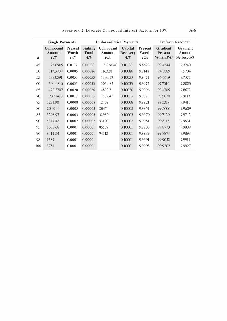
appendix 2: Discrete Compound Interest Factors for 10% A-6
45 72.8905 0.0137 0.00139 718.9048 0.10139 9.8628 92.4544 9.3740
50 117.3909 0.0085 0.00086 1163.91 0.10086 9.9148 94.8889 9.5704
55 189.0591 0.0053 0.00053 1880.59 0.10053 9.9471 96.5619 9.7075
60 304.4816 0.0033 0.00033 3034.82 0.10033 9.9672 97.7010 9.8023
65 490.3707 0.0020 0.00020 4893.71 0.10020 9.9796 98.4705 9.8672
70 789.7470 0.0013 0.00013 7887.47 0.10013 9.9873 98.9870 9.9113
75 1271.90 0.0008 0.00008 12709 0.10008 9.9921 99.3317 9.9410
80 2048.40 0.0005 0.00003 20474 0.10005 9.9951 99.5606 9.9609
85 3298.97 0.0003 0.00003 32980 0.10003 9.9970 99.7120 9.9742
90 5313.02 0.0002 0.00002 53120 0.10002 9.9981 99.8118 9.9831
95 8556.68 0.0001 0.00001 85557 0.10001 9.9988 99.8773 9.9889
96 9412.34 0.0001 0.00001 94113 0.10001 9.9989 99.8874 9.9898
98 11389 0.0001 0.00001 0.10001 9.9991 99.9052 9.9914
100 13781 0.0001 0.00001 0.10001 9.9993 99.9202 9.9927
Single Payments Uniform-Series Payments Uniform Gradient
n
Compound
Amount
F/P
Present
Worth
P/F
Sinking
Fund
A/F
Compound
Amount
F/A
Capital
Recovery
A/P
Present
Worth
P/A
Gradient
Present
Worth P/G
Gradient
Annual
Series A/G
die37039_ch20_ap2.indd A-6 2/25/08 7:22:14 PM

die37039_ch20_ap2.indd A-7 2/25/08 7:22:15 PM

Abbreviations and Acronyms
AHP Analytic Hierarchy Process ANSI American National Standards
Institute ASTM American Society for Testing
and Materials BOM Bill of Materials CAE Computer-Aided Engineering CR Customer Requirement CTQ Critical to Quality DBD Decision-Based Design DFA Design for Assembly DFE Design for the Environment DFM Design for Manufacture EC Engineering Characteristic FEA Finite Element Analysis FMEA Failure Modes and Effects
Analysis GD&T Geometric Dimensioning and
Tolerancing HOQ House of Quality ISO International Organization for
Standardization
JIT Just-in-Time LCC Life-cycle Costing MARR Minimum Attractive Rate of
Return MTBF Mean Time Between Failure NDE Nondestructive Evaluation NIST National Institute of Standards
and Technology OEM Original Equipment
Manufacturer PDP Product Design Process PDS Product Design SpeciJ cation PLM Product Life-cycle Management QFD Quality Function Deployment ROI Return on Investment RP Rapid Prototyping SPC Statistical Process Control TQM Total Quality Management TRIZ Theory of Inventive Problem
Solving USPTO United States Patent and
Trademark OfJ ce
die37039_ch99_ibc.indd 1 2/25/08 7:07:20 PM
