engineering fracture mechanicsuser.engineering.uiowa.edu/~rahman/efm_multiscale3d.pdf · spatially...

Engineering Fracture Mechanics 78 (2011) 27–46

Contents lists available at ScienceDirect

Engineering Fracture Mechanics

journal homepage: www.elsevier .com/locate /engfracmech

Stochastic multiscale fracture analysis of three-dimensionalfunctionally graded composites

Sharif Rahman a,⇑, Arindam Chakraborty b

a Department of Mechanical and Industrial Engineering, The University of Iowa, Iowa City, IA 52242, USAb Structural Integrity Associates, Inc., 5215 Hellyer Avenue, Suite 210, San Jose, CA 95138, USA

a r t i c l e i n f o a b s t r a c t

Article history:Received 9 October 2009Received in revised form 2 September 2010Accepted 13 September 2010Available online 19 September 2010

Keywords:Probabilistic fracture mechanicsPolynomial dimensional decompositionRandom microstructureReliability

0013-7944/$ - see front matter � 2010 Elsevier Ltddoi:10.1016/j.engfracmech.2010.09.006

⇑ Corresponding author. Tel.: +1 319 335 5679.E-mail address: [email protected]

A new moment-modified polynomial dimensional decomposition (PDD) method is pre-sented for stochastic multiscale fracture analysis of three-dimensional, particle-matrix,functionally graded materials (FGMs) subject to arbitrary boundary conditions. Themethod involves Fourier-polynomial expansions of component functions by orthonormalpolynomial bases, an additive control variate in conjunction with Monte Carlo simulationfor calculating the expansion coefficients, and a moment-modified random output toaccount for the effects of particle locations and geometry. A numerical verification con-ducted on a two-dimensional FGM reveals that the new method, notably the univariatePDD method, produces the same crude Monte Carlo results with a five-fold reduction inthe computational effort. The numerical results from a three-dimensional, edge-cracked,FGM specimen under a mixed-mode deformation demonstrate that the statisticalmoments or probability distributions of crack-driving forces and the conditional probabil-ity of fracture initiation can be efficiently generated by the univariate PDD method. Thereexist significant variations in the probabilistic characteristics of the stress-intensity factorsand fracture-initiation probability along the crack front. Furthermore, the results are insen-sitive to the subdomain size from concurrent multiscale analysis, which, if selectedjudiciously, leads to computationally efficient estimates of the probabilistic solutions.

� 2010 Elsevier Ltd. All rights reserved.

1. Introduction

In functionally graded materials (FGMs), the introduction of gradual changes in material compositions and microstruc-tures at the macroscale removes large-scale, interface-induced stress singularities that can otherwise lead to delaminationfailure [1]. However, due to formation of cracks during processing or service life, fracture remains an important failuremechanism. There are two major challenges in conducting fracture analyses of FGMs. First, an FGM is a multiphase,heterogeneous material with multiscale features, which, depending on the crack-tip location and microstructure, canhave markedly different crack-driving forces. Second, the microstructure of an FGM is inherently stochastic, which canbe modeled as a random field, describing random distributions of sizes, shapes, and orientations of constituent phases.Therefore, stochastic multiscale models are ultimately necessary to provide a realistic computational framework fordetermining mechanical performance of a crack, real or postulated, in an FGM.

Past computational works on FGM fracture are primarily driven by deterministic macroscopic models and entail mostlytwo-dimensional [2–4] and a few three-dimensional [5–7] media for calculating the stress-intensity factors (SIFs) from

. All rights reserved.

(S. Rahman).

http://dx.doi.org/10.1016/j.engfracmech.2010.09.006

mailto:[email protected]

http://dx.doi.org/10.1016/j.engfracmech.2010.09.006

http://www.sciencedirect.com/science/journal/00137944

http://www.elsevier.com/locate/engfracmech

28 S. Rahman, A. Chakraborty / Engineering Fracture Mechanics 78 (2011) 27–46

spatially varying elastic properties. In contrast, models of random microstructure or multiscale fracture analysis are few andfar between [8,9], and they mostly delve into two-dimensional FGMs. For instance, the authors recently developed a concur-rent multiscale model, which includes a stochastic description of a two-dimensional FGM microstructure and constituentmaterial properties, a two-scale algorithm including microscale and macroscale analyses for determining crack-drivingforces, and crude Monte Carlo simulation for fracture reliability analysis [9]. Numerical results indicate that the concurrentmultiscale model is sufficiently accurate, gives fracture probability solutions very close to those generated from the micro-scale (reference) model, and can reduce the computational effort of the latter model by a factor of more than two. However,the stochastic analysis in both multiscale and microscale models was conducted using crude Monte Carlo simulation, requir-ing tens of thousands of deterministic finite-element analyses (FEA) to estimate tail probabilities. In other words, the in-creased computational speed gained by the multiscale model is due to more efficient FEA in each deterministic sample,not stochastic analysis. Therefore, further research exploiting alternative stochastic methods – the principal objective of thiswork – should pave the way for probabilistic fracture analysis in a computationally efficient way. Developing such alterna-tive methods becomes indispensable when analyzing cracks in three-dimensional FGMs, as crude Monte Carlo simulation isno longer a viable option due to increased computational demand from three-dimensional FEA.

This paper presents a new moment-modified polynomial dimensional decomposition (PDD) method for stochastic mul-tiscale fracture analysis of three-dimensional, particle-matrix FGMs subject to arbitrary boundary conditions. The method isbased on (1) Fourier-polynomial expansions of component functions by orthonormal polynomial bases, (2) an additive con-trol variate in conjunction with Monte Carlo simulation for efficient calculation of the expansion coefficients, and (3) a mo-ment-modified random output to account for the effects of particle locations and geometry. Section 2 describes a generic,stochastic FGM fracture problem, defines random input parameters, and discusses crack-driving forces. Section 3 presentsa concurrent multiscale model for fracture analysis. Section 4 explores PDD, presents an efficient method for calculatingthe expansion coefficients, including a moment-modified random output, and discusses computational effort. The sectionalso includes numerical results from a two-dimensional FGM analysis, essentially verifying the PDD method. Section 5 illus-trates the capability of the proposed method by solving a three-dimensional FGM fracture problem, leading to the statisticalmoments and probability densities of crack-driving forces and the conditional probability of fracture initiation. Finally, theconclusions are drawn in Section 6.

2. Stochastic fracture problem

Consider a two-phase, functionally graded, heterogeneous solid with a planar crack, domain D � R3, and a schematicillustration of its microstructure, as shown in Fig. 1a. 1The microstructure includes two distinct material phases, phase p (greenor dark) and phase m (white or light), denoting particle and matrix constituents with subdomains Dp � D and Dm � D, respec-tively, where Dp [Dm ¼ D and Dp \Dm ¼ ;. Both constituents represent isotropic and linear-elastic materials, and the elasticitytensors of the particle and matrix, denoted by C(p) and C(m), respectively, are

1 For

CðiÞ :¼ miEi

ð1þ miÞð1� 2miÞ1� 1þ Ei

ð1þ miÞI; i ¼ p;m; ð1Þ

where the symbol � denotes the tensor product; Ei and mi are the elastic modulus and Poisson’s ratio, respectively, of phase i;and 1 and I are second- and fourth-rank identity tensors, respectively. The superscripts or subscripts i = p and i = m refer toparticle and matrix, respectively. At a spatial point x 2 D in the macroscopic length scale, let /p(x)and /m(x) denote the vol-ume fractions of the particle and matrix, respectively. Each volume fraction is bounded between 0 and 1 and satisfies theconstraint /p(x) + /m(x) = 1. The crack faces are traction-free, and there is perfect bonding between the matrix and particles.In addition, no porosities are included in the matrix or particle phases.

For a quasi-static, elastic problem with small displacements and strains, the variational or weak form of the equilibriumequation and boundary conditions is

ZD

ðCðxÞ : �Þ : d�dD�ZD

b � dudD�Z

Ct

�t � dudC�X

xK2Cu

f ðxKÞ � duðxKÞ �X

xK2Cu

df ðxKÞ � uðxKÞ � �uðxKÞ½ � ¼ 0; ð2Þ

where u : D! R3 is the displacement vector; C(x) and � :¼ ð1=2Þð$þ $TÞu denote the spatially variant elasticity tensorand strain tensor, respectively; Ct and Cu are two disjoint portions of the boundary C, where the traction vector �t anddisplacement �u are prescribed, respectively; fT(xK) is the vector of reaction forces at a constrained node K on Cu; $T :¼f@=@x1; @=@x2; @=@x3g is the vector of gradient operators; and symbols ‘‘.”, ‘‘:”, and d denote dot product, tensor contraction,and variation operator, respectively. The discretization of the weak form, Eq. (2), depends on how the elasticity tensor C(x) isdefined, i.e., how the elastic properties of constituent material phases and their gradation characteristics are described.Nonetheless, a numerical method, e.g., the finite-element method, is generally required to solve the discretized weak form,providing various response fields of interest.

interpretation of color in Figs. 1 and 3–10, the reader is referred to the web version of this article.

on uu Γ

Fig. 1. Schematics of a two-phase, three-dimensional FGM fracture problem: (a) a planar crack subject to arbitrary boundary conditions; (b) a concurrentmultiscale model; and (c) a small, bounded subdomain of a crack tip. Note: D = domain of the entire solid, D = subdomain with explicit microstructure,D� = small subdomain surrounding a crack tip on the crack front.

S. Rahman, A. Chakraborty / Engineering Fracture Mechanics 78 (2011) 27–46 29

2.1. Random input

Uncertainties in input to FGM fracture analysis leading to statistical characteristics of SIFs come from a variety of sources.Two important sources considered in this work are: (1) random microstructure, including uncertainties in the volume frac-tion, number, and locations of particles and (2) random elastic material properties of constituents. They are briefly describedas follows.

2.1.1. Random microstructure2.1.1.1. Particle volume fraction. The particle volume fraction /p(x) can be modeled as an inhomogeneous (non-stationary), non-Gaussian, random field, which has mean lp(x) and standard deviation rp(x) [10]. The standardized particle volume fraction

~/pðxÞ :¼/pðxÞ � lpðxÞ

rpðxÞ; ð3Þ

which has zero mean and unit variance, is at least a weakly homogeneous (stationary) random field with prescribed covariancefunction C~/p

ðsÞ :¼ E ~/pðxÞ~/pðxþ sÞh i

, where E is the expectation operator, and with marginal cumulative distribution functionFpð~/pÞ such that 0 6 /p(x) 6 1 with probability one. If the covariance function C~/p

ðsÞ is appropriately bounded, the standard-ized phase volume fraction can be viewed as a translation random field ~/pðxÞ ¼ Gp½apðxÞ� :¼ F�1

p ½UðapðxÞÞ�, where Gp is a map-ping of the Gaussian field on a non-Gaussian field, ap(x) is the Gaussian image field, and U(�) is the distribution function of astandard Gaussian random variable. Subsequently, the Karhunen–Loéve approximation of the image field leads to [10]

~/pðxÞ ffi Gp

XM

k¼1

Zp;k

ffiffiffiffiffiffiffikp;k

pWp;kðxÞ

" #; ð4Þ


where kp,k and Wp,k(x) denote the kth eigenvalue and the kth eigenfunction, respectively, of the covariance function of ap(x),and Zp,k is an independent copy of a standard Gaussian random variable. According to Eq. (4), the Karhunen–Loéve approx-imation yields a parametric representation of the standardized phase volume fraction ~/pðxÞ and, hence, of /p(x) with MGaussian variables. The random field description of /p(x) allows the particle volume fraction to have random fluctuationsat a point x in the macroscopic length scale.

2.1.1.2. Particle number and locations. The random microstructure entailing particle locations can be described using the well-known Poisson random field. However, since the FGM microstructure varies spatially, the Poisson field must be inhomoge-neous. Consider an inhomogeneous Poisson field NðD0Þ with an intensity measure lD0 :¼

RD0 kðxÞdx, where x 2 D0 � R3 is a

spatial coordinate, k(x) P 0 is a spatially variant intensity function, and D0 2 R3 is a bounded subset of R3 such that pointsof N falling in R3 nD0 do not contribute to particles in D. The Poisson point field has the following properties: (1) the numberNðD0Þ of points in a bounded subset D0 has a Poisson distribution with intensity measure lD0 ; and (2) random variablesNðD01Þ; . . . ; NðD0KÞ for any integer K P 2 and disjoint sets D01; . . . ;D0K are statistically independent. The Poissonfield NðD0Þ gives the number of points in D0 and is characterized by the probability,

P NðD0Þ ¼ n½ � ¼RD0 kðxÞdx

� �n

n!exp �

ZD0

kðxÞdx� �

; n ¼ 0;1;2; . . . ; ð5Þ

that n Poisson points exist in D0. An FGM with fully penetrable spherical particles that have the same deterministic size, asassumed in this work, and a deterministic particle volume fraction up(x) has the intensity function [11]

kðxÞ ffi 1Vp

ln1

1�upðxÞ

" #; x 2 D0; ð6Þ

where Vp is the common volume of the particles. When /p(x) is a random field, as treated in this work, up(x) can be viewed asa sample function of /p(x). For more complex microstructures comprising random particle geometry, no such closed-formrelationships exist, but they can be formulated algorithmically [12].

2.1.1.3. Mosaic random field. A random point field, known as the mosaic random field [13] and employing an inhomogeneousPoisson field, can be used to model particle-matrix FGMs. Once the intensity function has been determined, samples of syn-thetic microstructures of two-phase FGMs are generated from the mosaic random field based on the following algorithm:

� Step 1: Define bounded subsets D and D0 of R3. The bounded subset D0 must be such that points of N falling in R3 nD0 donot contribute to particles in D.� Step 2: Generate a sample up(x) of the random particle volume fraction /p(x) using Eqs. (3) and (4). Calculate the corre-

sponding sample k(x) of the random intensity function from Eq. (6).� Step 3: Generate a sample k* of the homogeneous Poisson random variable NðD0Þ, which has a constant intensity

k ¼maxx2R3 kðxÞ, where k(x) is a bounded intensity function in D0.� Step 4: Generate k* independent samples of uniformly distributed points (ui,1,ui,2,ui,3) in D0. Denote these points by xi,

i = 1, . . . ,k*.� Step 5: Perform thinning of the point set obtained in Step 4. In so doing, each point xi, independently of the other, is kept

with probability k(xi)/k*, which is equivalent to discarding the point with probability 1 � k(xi)/k*. The resulting point pat-tern with the size k 6 k* follows the inhomogeneous Poisson field NðD0Þ with the intensity function k(x). Let these pointsbe denoted by Ci, i = 1, . . . ,k.� Step 6: Place particles with their centroids coincident with the points Ci, i = 1, . . . ,k. The resultant subsets Dp and Dm of

the particle and matrix regions, respectively, of D produce a sample of a two-phase, statistically inhomogeneousmicrostructure.

Independent samples of an FGM random microstructure are delivered by repeated application of the above algorithm.

2.1.2. Random constituent material propertiesIn addition to a spatially variant random volume fraction of particles leading to a random microstructure, the constituent

properties of material phases can also be stochastic. Let Ep and mp denote the elastic modulus and Poisson’s ratio, respectively,of the particle, and Em and mm denote the elastic modulus and Poisson’s ratio, respectively, of the matrix. Therefore, the ran-dom vector fEp; Em; mp; mmgT 2 R4 describes the stochastic elastic properties of both constituents. Unlike volume fractions,however, the constituent properties are spatially invariant in the macroscopic length scale.

In summary, the input uncertainties include: (1) M random variables Zp,1, . . . ,Zp,M due to the discretization of the randomfield /p(x); (2) a Poisson random variable N and resulting 3N random variables ðUi;1;Ui;2;Ui;3Þ; i ¼ 1; . . . ;N, representingcoordinates of the particle centroids in D0; and (3) four random constituent properties Ep, Em, mp, mm. In other words, an inputrandom vector R ¼ fZp;1; . . . ; Zp;M;N; ðU1;1;U1;2;U1;3Þ; . . . ; ðUN;1;UN;2;UN;3Þ; Ep; Em; mp; mmgT 2 RN characterizes uncertaintiesfrom all sources in an FGM, where the dimension N ¼ M þ 3Nþ 5 is an integer-valued random variable and is completelydescribed by its joint probability density function (PDF) fR(r), where r is a realization of R.


2.2. Crack-driving forces and reliability

A major objective of stochastic fracture-mechanics analysis is to find probabilistic characteristics of crack-driving forces,such as SIFs KI(R), KII(R), and KIII(R) for modes I–III, respectively, due to random input R. For a given input sample, a standardFEA solves the discretized weak form (Eq. (2)), leading to the calculation of SIFs by standard interaction integrals [14].

Let y(R) describe a generic crack-driving force or a relevant performance function involving SIFs for a given FGM fractureproblem of interest. Suppose that a failure is defined when the crack propagation is initiated at a crack tip on the crack front,i.e., when the effective SIF Keff ðRÞ ¼ �hðKIðRÞ;KIIðRÞ;KIIIðRÞÞ > KIc , where �h depends on the selected mixed-mode fracture cri-terion [15] and KIc is a relevant mode-I fracture toughness of the material measured in terms of SIF. This requirement cannotbe satisfied with certainty, since KI, KII, and KIII are all dependent on R, which is random, and KIc itself may be a random var-iable or field. Hence, the fracture performance of an FGM should be evaluated by the conditional reliability or its comple-ment, the conditional probability of fracture initiation PF(KIc), defined as the multifold integral

PFðKIcÞ :¼ P½yðRÞ < 0� :¼Z

RNIyðrÞfRðrÞdr; ð7Þ

where

yðRÞ ¼ KIc � �h KIðRÞ;KIIðRÞ;KIIIðRÞð Þ ð8Þ

is a multivariate performance function that depends on the random input R and IyðrÞ is an indicator function such thatIyðrÞ ¼ 1 if yðrÞ < 0 and IyðrÞ ¼ 0 if yðrÞ > 0. The evaluation of the multidimensional integral in Eq. (7), either analyticallyor numerically, is not possible because the total number of random variables N is large, fR(r) is generally non-Gaussian,and y(r) is a highly nonlinear function of r. Crude Monte Carlo simulation to estimate the fracture-initiation probability iscomputationally burdensome, if not prohibitive; therefore, alternative stochastic methods are essential for providing bothaccurate and efficient solutions.

The effort in conducting probabilistic fracture analysis of FGM is influenced by two primary sources: (1) deterministiccomputing of SIFs, which requires expensive FEA for a given input sample and (2) stochastic computing of SIFs, which in-volves uncertainty propagation in a high-dimensional stochastic system. A new moment-modified PDD method in conjunc-tion with a concurrent multiscale fracture model developed in this work reduces computational demand from both sources.

3. Concurrent multiscale analysis

The FGM microstructure schematically illustrated in Fig. 1a contains discontinuities in material properties at the inter-faces between the matrix and particles. At the crack-front region, discrete material property information derived from themicrostructure is required for calculating the crack-tip fields accurately. However, far away from the crack-front, wherethe effect of the crack-tip singularity vanishes rapidly, individual constituent material properties may not be needed, andan appropriately derived continuous, effective material property should suffice. Therefore, a concurrent multiscale analysis,where the material representation is discrete at the crack-front region and continuous elsewhere, leading to a combinedmicromechanical and macromechanical stress analysis should provide a more efficient solution of crack-tip fields than amicroscale analysis that is solely based on discrete material representation everywhere.

As depicted in Fig. 1b, consider an arbitrary, three-dimensional, bounded subdomain D#D surrounding the crack front.The number of particles falling in D0 is N :¼NðD0Þ, where D0 � R3 is a bounded subset such that points of N falling inR3 nD0 do not contribute to particles in D. The integer-valued random variable N also follows a Poisson distribution withthe same intensity function k(x) derived from Eq. (6). The subdomain D, once defined, is statistically filled with particles,whereas the remaining subdomain D nD is assigned a continuously varying effective elasticity tensor CðxÞ, obtained froma suitable micromechanical homogenization [16]. According to the concurrent multiscale model, Eq. (2) is discretized andsolved using

CðxÞ ffiCðpÞ; if x 2 D and x 2 Dp

� �;

CðmÞ; if x 2 D and x 2 Dm� �

;

CðxÞ; if x 2 D nD;

8>><>>: ð9Þ

where discontinuity in material properties at the interfaces between D and D nD and between Dp and Dm exist, renderingcalculation of SIF difficult. To overcome this problem, consider a small, bounded subdomain D� � D surrounding a crack tipof interest with coordinate xtip, depicted in Fig. 1c, such that material properties of either the particle or the matrix phase areassigned in D�. The result is a slight modification of the elasticity tensor, for instance,

CðxÞ ffiCðpÞ; if x 2 D� and xtip 2 Dp

� �or if x 2 D nD� and x 2 Dp

� �;

CðmÞ; if x 2 D� and xtip 2 Dm� �

or if x 2 D nD� and x 2 Dm� �

;

CðxÞ; if x 2 D nD;

8>><>>: ð10Þ


yielding a locally homogeneous material representation, i.e., C(x) is either C(p) or C(m), but constant for x 2 D�. Consequently,the mixed-mode SIFs at that crack tip ðxtip 2 D�Þ are readily calculated from [14,17]

Ki ffi12 Mð1;iÞ

p Ep; if xtip 2 Dp;

12 Mð1;iÞ

m Em; if xtip 2 Dm;

(; i ¼ I; II; ð11Þ

and

KIII ffiMð1;IIIÞ

p lp; if xtip 2 Dp;

Mð1;IIIÞm lm; if xtip 2 Dm;

(ð12Þ

where Mð1;iÞp and Mð1;iÞ

m are the associated interaction integrals for mode i (i = I, II, III), when CðxÞ ¼ CðpÞ; x 2 D� andCðxÞ ¼ CðmÞ; x 2 D�, respectively, provided that their domains of integration lie within D�. For plane stress conditions,Ej ¼ Ej, and for plane strain conditions or three-dimensional problems, Ej ¼ Ej=ð1� m2

j Þ, where Ej denotes the elastic modu-lus, mj denotes the Poisson’s ratio, and lj = Ej/2(1 + mj) is the shear modulus. The subscripts j = p and j = m refer to particle andmatrix, respectively. Since the interaction integrals vary along the crack front, the SIFs also depend on the crack-tip location.In Eq. (10), the size of D� should be comparable to the microstructural length scale but large enough for the interaction inte-grals and SIFs to be calculated accurately. Further details of the concurrent multiscale model, including verification with afull microscale model, are available in the authors’ prior work on two-dimensional FGMs [9].

The stochastic analysis employing the concurrent multiscale model has the random input vector R ¼ fZp;1; . . . ;

Zp;M ;N; ðU1;1;U1;2;U1;3Þ; . . . ; ðUN;1;UN;2;UN;3Þ; Ep; Em; mp; mmgT 2 RN , where N ¼ M þ 3Nþ 5. If D � D, then N <N, resultingin a dimension reduction in stochastic multiscale analysis.

4. Moment-modified polynomial dimensional decomposition method

Let ðX;F; PÞ be a complete probability space, where X is a sample space, F is a r-field on X, and P : F! ½0;1� is a prob-ability measure. With BN representing the Borel r-field on RN , consider an RN-valued independent random vectorfR ¼ fR1; . . . ;RNgT : ðX;FÞ ! ðRN ;BNÞg, which describes uncertain input from the FGM microstructure and constituent elas-tic properties described in the preceding section. The probability law of R is completely defined by the joint PDFfRðrÞ ¼ Pi¼N

i¼1 fiðriÞ, where fi(ri) is the PDF of Ri defined on the corresponding probability triple ðXi;Fi; PiÞ. Let L2ðXi;Fi; PiÞbe a Hilbert space that is equipped with a set of complete orthonormal bases {wij(ri); j = 0,1, . . .}, which is consistent withthe probability measure of Ri. For example, classical orthonormal polynomials, including Hermite, Legendre, and Jacobi poly-nomials, can be used when Ri follows Gaussian, uniform, and Beta probability distributions, respectively [18].

Let y(R), a real-valued, measurable transformation on ðX;FÞ, define a SIF or relevant performance function that dependson the SIFs of a given FGM fracture problem. Using orthonormal polynomial bases and Fourier-polynomial expansions ofcomponent functions, an S-variate (1 6 S 6 N) approximation from the PDD of y(R) is [18]

~ySðRÞ ffi y0 þXN

i¼1

Xm

j¼1

aijwijðRiÞ þXN

i1 ;i2¼1;i1<i2

Xm

j2¼1

Xm

j1¼1

bi1 i2 j1 j2wi1 j1ðRi1 Þwi2 j2

ðRi2 Þ þ � � � þXN

i1 ;...;iS¼1;i1<��<iS

Xm

jS¼1

� � �Xm

j1¼1

Ci1 ��iS j1 ��jS

YS

s¼1

wis jsðRis Þ; ð13Þ

where

y0 :¼Z

RNyðrÞfRðrÞdr ¼ E½yðRÞ�; ð14Þ

aij :¼Z

RNyðrÞwijðriÞfRðrÞdr ¼ E½yðRÞwijðRiÞ�; ð15Þ

bi1 i2 j1j2:¼Z

RNyðrÞwi1 j1

ðri1 Þwi2 j2ðri2 ÞfRðrÞdr ¼ E½yðRÞwi1 j1

ðRi1 Þwi2 j2ðRi2 Þ�; ð16Þ

..

.

Ci1 ��iS j1 ��jS ¼Z

RNyðrÞ

YS

s¼1

wis jsðris ÞfRðrÞdr ¼ E yðRÞ

YS

s¼1

wis jsðRis Þ

" #ð17Þ

are the expansion coefficients and 1 6m 61 is the largest order of orthogonal polynomials. The right side of Eq. (13), forS = N, converges to y(R) in the mean square sense as m ?1. Once the embedded coefficients y0; aij; bi1 i2j1 j2

; . . . ; Ci1 ��iSj1 ��jS


are calculated, as described in a forthcoming section, Eq. (13) furnishes an approximate but explicit map ~yS : RN ! R that canbe viewed as a surrogate of the exact map y : RN ! R, which describes the input-output relationship from the FGM fracture-mechanics simulation. Therefore, any probabilistic characteristic of y(R), including its statistical moments and fracture-initiation probabilities, can be easily estimated by performing Monte Carlo simulation of ~ySðRÞ rather than that of y(R).

4.1. Calculation of coefficients

4.1.1. Monte carlo simulationConsider L independent samples rðlÞ ¼ rðlÞ1 ; . . . ; rðlÞN

n oT2 RN; l ¼ 1; . . . ; L of the input vector R that can be generated to esti-

mate the coefficients

y0 ffi1L

XL

l¼1

y rðlÞ� �

; ð18Þ

aij ffi1L

XL

l¼1

y rðlÞ� �

wij rðlÞi

� �; ð19Þ

bi1 i2 j1j2ffi 1

L

XL

l¼1

y rðlÞ� �

wi1 j1rðlÞi1

� �wi2 j2

rðlÞi2

� �; ð20Þ

..

.

Ci1 ��iSj1 ��jS ffi1L

XL

l¼1

y rðlÞ� �YS

s¼1

wisjsrðlÞis

� �: ð21Þ

Therefore, Eq. (13) becomes

~ySðRÞ ffi1L

XL

l¼1

y rðlÞ� �

þXN

i¼1

Xm

j¼1

1L

XL

l¼1

y rðlÞ� �

wij rðlÞi

� � !wijðRiÞ þ

XN

i1 ;i2¼1;i1<i2

Xm

j2¼1

Xm

j1¼1

1L

XL

l¼1

y rðlÞ� �

wi1j1rðlÞi1

� �wi2 j2

rðlÞi2

� � !wi1 j1ðRi1 Þwi2 j2

ðRi2 Þ þ � � �

þXN

i1 ;...;iS¼1;i1<��<iS

Xm

jS¼1

� � �Xm

j1¼1

1L

XL

l¼1

y rðlÞ� �YS

s¼1

wisjsrðlÞis

� � !YS

s¼1

wis jsðRis Þ; ð22Þ

generating the univariate or bivariate approximation of y(R) by selecting S = 1 or S = 2, respectively.The Monte Carlo integration to calculate the coefficients is approximate when L <1 and the standard errors in calculating

the coefficients are proportional to the standard deviations of the integrands given in Eqs. (14)–(17) divided byffiffiffiLp

[19].Therefore, the error by Monte Carlo integration can be reduced by either increasing the sample size L or decreasing the var-iance of the integrand. If random sampling of the integrand produces a large variance (e.g., when y has rapid changes in thedomain of interest, especially in sign), the error becomes unacceptably large. Therefore, depending on the nature of the func-tion y, additional samples are required to achieve reduced error. Since an FGM fracture analysis requires expensive finite-element calculations to obtain samples of y(R) for given samples of random input, increasing the sample size may renderthe calculation of coefficients prohibitively expensive. Another way to improve the accuracy of Monte Carlo integration witha relatively small number of samples is to reduce the variance of the integrand. In this work, an additive control variatemethod [19,20] was utilized toward this end.

4.1.2. Control variateConsider a multivariate integral for the determination of the coefficients in Eqs. (15)–(17). For example, using the additive

control variate technique, aij in Eq. (15) can be rewritten as

aij ¼Z

RNyðrÞ � hðrÞ½ �wijðriÞfRðrÞdr þ

ZRN

hðrÞwijðriÞfRðrÞdr; ð23Þ

where h(r) is a control variate such that (1) y(r) and h(r) are similar over the entire domain of integration and (2) the integralRRN hðrÞwijðriÞfRðrÞdr can be obtained analytically. The first term in Eq. (23) has a small variance when y(r) and h(r) are lin-

early related through

hðrÞ ¼ yðrÞ þ b; ð24Þ
where b is a constant. Assuming that the second term in Eq. (23) is known analytically, the variance in Eq. (23) comes onlyfrom the first term. Since y(r) and h(r) are similar, i.e., b � 0, one can expect the variance of [y(R) � h(R)]wij(Ri) to be less thanthe variance of y(R)wij(Ri). Using Monte Carlo integration to evaluate the first integration in Eq. (23) yields
aij ffi1L

XL

l¼1

y rðlÞ� �

� h rðlÞ� �

wij rðlÞi

� �þZ

RNhðrÞwijðriÞfRðrÞdr; ð25Þ


which is expected to give better accuracy than that given by Eq. (19). However, for any arbitrary function y(r), there is nogeneral way to find an analytical expression for h(r), and it may even be impossible. Therefore, the use of Eq. (25) employingan analytical expression for h(r) is often not practical, especially when y(r) is obtained implicitly from FEA.

An alternative approach is to exploit the PDD of y(r) to approximate h(r). In this regard, consider an S-variate approxima-tion of y(r) to generate the qth approximation

hðqÞðr; NÞ ¼ y0 þXN

i¼1

Xm

j¼1

aðqÞij wijðriÞ þXN

i1 ;i2¼1;i1<i2

Xm

j2¼1

Xm

j1¼1

bðqÞi1 i2j1 j2wi1 j1ðri1 Þwi2 j2

ðri2 Þ þ � � �

þXN

i1 ;...;iS¼1;i1<��<iS

Xm

jS¼1

� � �Xm

j1¼1

CðqÞi1 ��iSj1 ��jS

YS

s¼1

wis jsðris Þ ð26Þ

of h(r), where the argument N of h(q) denotes the total number of random variables involved (upper limit of the outer sums)and q = 0,1,2, . . .. Then, the estimated coefficients are

aðqÞij ¼1L

PLl¼1

y rðlÞ� �

wij rðlÞi

� �; if q ¼ 0;

1L

PLl¼1

y rðlÞ� �

� hðq�1Þ rðlÞ; N� �h i

wij rðlÞi

� �þ aðq�1Þ

ij ; if q ¼ 1;2; . . . ;

8>><>>: ð27Þ

bðqÞi1 i2j1 j2¼

1L

PLl¼1

y rðlÞ� �

wi1 j1rðlÞi1

� �wi2 j2

rðlÞi2

� �; if q ¼ 0;

1L

PLl¼1

y rðlÞ� �

� hðq�1Þ rðlÞ; N� �h i

wi1j1rðlÞi1

� �wi2 j2

rðlÞi2

� �þ bðq�1Þ

i1 i2j1 j2; if q ¼ 1;2; . . . ;

8>>><>>>:

ð28Þ

..

.

CðqÞi1 ��iS j1 ��jS¼

1L

PLl¼1

y rðlÞ� � QS

s¼1wis js

rðlÞis

� �; if q ¼ 0;

1L

PLl¼1

y rðlÞ� �

� hðq�1Þ rðlÞ; N� �h i QS

s¼1wis js

rðlÞis

� �þ Cðq�1Þ

i1 ��iS j1 ��jS; if q ¼ 1;2; . . . :

8>>><>>>:

ð29Þ

With each new iteration in Eq. (26), jy(r) � h(r)j decreases as the coefficients are corrected based on the difference between

y(r) and h(r). When y(r) = h(r), the first terms in Eqs. (27)–(29) become zero for q > 0 and no further iteration is necessary.

Therefore, the iteration can be terminated by the conditions aðqÞij � aðq�1Þij

�� < �; bðqÞij � bðq�1Þij

�� < �; . . . ; CðqÞi1 ��iSj1 ��jS�

��Cðq�1Þ

i1 ��iSj1 ��jSj < �, where � is a user-defined tolerance. Note that the same samples of y(R) are used in all iterations, requiring

no additional response calculations. Therefore, converged values of the expansion coefficients from Eqs. (27)–(29) areobtained with little additional effort.

4.2. Moment modification

The stochastic fracture analysis employing the concurrent multiscale model involves the random input vectorR ¼ fZp;1; . . . ; Zp;M;N; ðU1;1;U1;2;U1;3Þ; . . . ; ðUN;1;UN;2;UN;3Þ; Ep; Em; mp; mmgT 2 RN , where finding the PDF for the particle loca-tion coordinates fðUi;1;Ui;2;U1;3Þg; i ¼ 1; . . . ;N is not trivial. Therefore, a straightforward application of the PDD method isvery difficult, if not impossible, as the method requires orthonormal bases corresponding to the PDF of all input random vari-ables involved. An alternative but approximate approach, referred to as the moment-modified polynomial dimensional decom-position method, was developed to circumvent this problem, and is described as follows.

Recall that y(r) = y(r1, . . .,rN) represents either a SIF or a performance function that depends on SIFs. In general, the objec-tive is to evaluate the probabilistic characteristics of a generic output response yðRÞ 2 R, when the probability distribution ofthe random input R 2 RN is prescribed. The newly developed moment-modified PDD method for stochastic fracture analysisof FGMs involves the following three-step algorithm:

� Step 1: Generate L samples y(r(l)), l = 1, . . .,L, of the random output y(R) by employing the concurrent multiscale fracturemodel described in Section 3. The output samples y(r(l)), l = 1, . . .,L, contain effects of all random variables, including par-ticle locations considered in the multiscale model.� Step 2: Define R ¼ fZp;1; . . . ; Zp;M; Ep; Em; mp; mmgT 2 RN; N ¼ M þ 4 as the truncated input random vector, which excludes

variables describing particle locations. Using L samples of y(R) from Step 1 and a truncated control variate hðqÞð�r; NÞ inEq. (26), calculate the PDD coefficients from Eqs. (27)–(29) for i; i1; i2; i3; . . . ¼ 1; . . . ; N and j, j1, j2, j3, . . . = 1, . . ., m.Therefore, the N-truncation of the S-variate polynomial decomposition becomes


�ySðRÞ ¼1L

XL

l¼1

y rðlÞ� �

þXN

i¼1

Xm

j¼1

1L

XL

l¼1

y rðlÞ� �

wij �rðlÞi

� � !wijðRiÞ þ

XN

i1 ;i2¼1;i1<i2

Xm

j2¼1

Xm

j1¼1

1L

XL

l¼1

y rðlÞ� �

wi1j1�rðlÞi1

� �wi2 j2

�rðlÞi2

� � !wi1 j1ðRi1 Þwi2 j2

ðRi2 Þ þ � � �

þXN

i1 ;...;iS¼1;i1<��<iS

Xm

jS¼1

� � �Xm

j1¼1

1L

XL

l¼1

y rðlÞ� �YS

s¼1

wisjs�rðlÞis

� � !YS

s¼1

wis jsðRis Þ: ð30Þ

Since R is a subvector of R; �ySðRÞ cannot fully capture the effect of the variability from particle locations.� Step 3: Estimate the mean-variance pairs

l :¼ E½yðRÞ� ffi 1L

XL

l¼1

y rðlÞ� �

; r2 :¼ E½yðRÞ � l�2 ffi 1L

XL

l¼1

y rðlÞ� �

� l 2 ð31Þ

and

�l :¼ E½�ySðRÞ� ffi1L

XL

l¼1

�yS �rðlÞ� �

; �r2 :¼ E½�ySðRÞ � �l�2 ffi 1L

XL

l¼1

�yS �rðlÞ� �

� �l 2 ð32Þ

of y(R) and �ySðRÞ, respectively, both calculated from the existing samples of y(R). Postulate that the sample properties ofð~yS � lÞ=r and ð�yS � �lÞ=�r are the same, yielding yet another approximation,

~ySðRÞ ffi lþ r�r

�ySðRÞ � ~l

; ð33Þ

without requiring additional FEA.

Eq. (33) provides a heuristic, but convenient, approximation of ~ySðRÞ in Eq. (22) without having to include orthonormalpolynomial bases associated with random particle locations.

Since the material at a crack tip (xtip) on the crack front can either be that of the particle or the matrix with a possiblysignificant mismatch between constituent properties, jumps (discontinuities) may occur in a relevant fracture response.Therefore, two separate stochastic analyses, one with the crack tip in the particle phase and the other with the crack tipin the matrix phase, are required for the moment-modified PDD method. Consider two variants of ~ySðRÞ; ~yS;pðRÞ and~yS;mðRÞ, and their N-truncated S-variate approximations, �yS;pðRÞ and �yS;mðRÞ, that can be generated depending on whetherthe crack tip is in the particle or in the matrix, respectively. Correspondingly, let lp;r2

p;lm;r2m; �lp; �r2

p; and �lm; �r2m be the

pairs of second-moment statistics of ~yS;pðRÞ; ~yS;mðRÞ; �yS;pðRÞ, and �yS;mðRÞ, respectively. Then, an S-variate approximation ofa discontinuous stochastic response from FGM fracture analysis becomes

~ySðRÞ ffilp þ

rp�rp

�yS;pðRÞ � ~lp

; if xtip 2 Dp;

lm þ rm�rm

�yS;mðRÞ � ~lm

; if xtip 2 Dm:

(ð34Þ

By Monte Carlo sampling of ~ySðRÞ in Eq. (34), the probabilistic characteristics of SIFs, including the conditional probability offracture initiation, can be easily estimated. This sampling should not be confused with crude Monte Carlo simulation, whichrequires finite-element calculation of y(r(l)) for any input sample r(l) and can, therefore, be expensive or even prohibitive,particularly when the sample size needs to be very large for estimating small probabilities. In contrast, the Monte Carlo sim-ulation embedded in the PDD method requires evaluations of simple analytical functions that stem from an S-variate approx-imation ~ySðRÞ. Therefore, an arbitrarily large sample size can be accommodated in the PDD method.

4.3. Computational effort

The moment-modified PDD method using the additive control variate requires finite-element evaluations of L samplesy(r(l)); l = 1, . . ., L, of y(R) to determine the coefficients y0; aij; bi1 i2j1 j2

; . . ., for i; i1; i2; . . . ¼ 1; . . . ; N and j, j1, j2, . . . = 1, . . .,m. The iterative scheme involving the additive control variate for estimating the expansion coefficients does not requireadditional samples of y(R). Therefore, the computational effort required by the proposed method comes primarily from con-ducting L FEA. However, due to the discrete nature of material property at a crack tip on the crack front, L samples or FEA arerequired for each of two stochastic fracture analyses – one for the matrix material at the crack tip and other for the particlematerial at the crack tip. Therefore, a total of 2L output samples or FEA are required by the proposed method.

For a generic stochastic problem, pre-selecting the sample size L is not easy. Therefore, progressively larger values of Lshould be tried in order to determine the minimum value of L. Furthermore, L depends on S in the S-variate approximation.From the authors’ experiences, L increases with S. Therefore, a larger sample size should be expected for the bivariate (S = 2)approximation than for the univariate (S = 1) approximation.


4.4. Verification

The moment-modified PDD method provides approximate solutions; therefore, an evaluation of its accuracy with respectto a reference solution – for instance, the results from crude Monte Carlo simulation – is necessary. Since crude Monte Carlosimulation is not practical for analyzing three-dimensional media, a two-dimensional FGM specimen, previously examinedby the authors [9], was selected to conduct the verification.

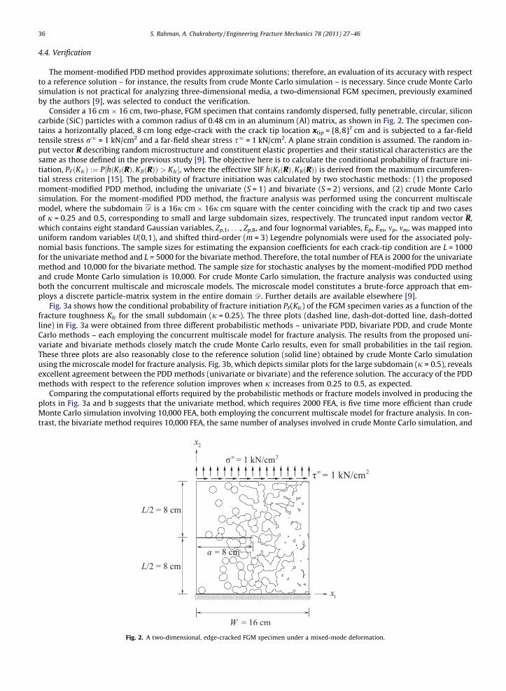
Consider a 16 cm 16 cm, two-phase, FGM specimen that contains randomly dispersed, fully penetrable, circular, siliconcarbide (SiC) particles with a common radius of 0.48 cm in an aluminum (Al) matrix, as shown in Fig. 2. The specimen con-tains a horizontally placed, 8 cm long edge-crack with the crack tip location xtip = {8,8}T cm and is subjected to a far-fieldtensile stress r1 = 1 kN/cm2 and a far-field shear stress s1 = 1 kN/cm2. A plane strain condition is assumed. The random in-put vector R describing random microstructure and constituent elastic properties and their statistical characteristics are thesame as those defined in the previous study [9]. The objective here is to calculate the conditional probability of fracture ini-tiation, PFðKIcÞ :¼ P½�hðKIðRÞ;KIIðRÞÞ > KIc�, where the effective SIF �hðKIðRÞ;KIIðRÞÞ is derived from the maximum circumferen-tial stress criterion [15]. The probability of fracture initiation was calculated by two stochastic methods: (1) the proposedmoment-modified PDD method, including the univariate (S = 1) and bivariate (S = 2) versions, and (2) crude Monte Carlosimulation. For the moment-modified PDD method, the fracture analysis was performed using the concurrent multiscalemodel, where the subdomain D is a 16j cm 16j cm square with the center coinciding with the crack tip and two casesof j = 0.25 and 0.5, corresponding to small and large subdomain sizes, respectively. The truncated input random vector R,which contains eight standard Gaussian variables, Zp,1, . . ., Zp,8, and four lognormal variables, Ep, Em, mp, mm, was mapped intouniform random variables U(0,1), and shifted third-order (m = 3) Legendre polynomials were used for the associated poly-nomial basis functions. The sample sizes for estimating the expansion coefficients for each crack-tip condition are L = 1000for the univariate method and L = 5000 for the bivariate method. Therefore, the total number of FEA is 2000 for the univariatemethod and 10,000 for the bivariate method. The sample size for stochastic analyses by the moment-modified PDD methodand crude Monte Carlo simulation is 10,000. For crude Monte Carlo simulation, the fracture analysis was conducted usingboth the concurrent multiscale and microscale models. The microscale model constitutes a brute-force approach that em-ploys a discrete particle-matrix system in the entire domain D. Further details are available elsewhere [9].

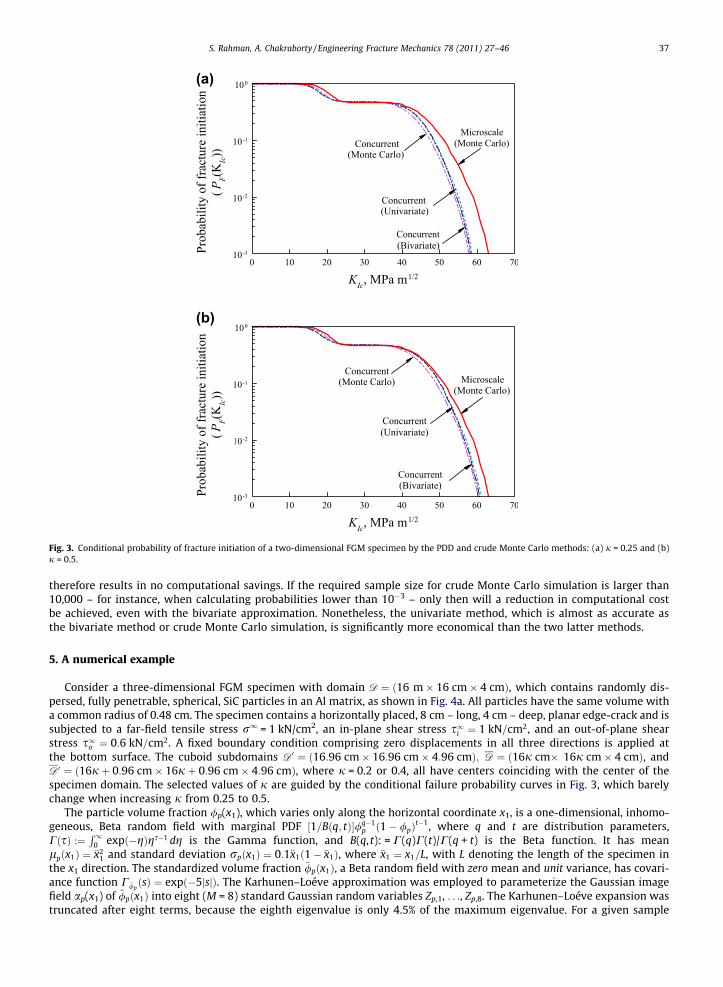
Fig. 3a shows how the conditional probability of fracture initiation PF(KIc) of the FGM specimen varies as a function of thefracture toughness KIc for the small subdomain (j = 0.25). The three plots (dashed line, dash-dot-dotted line, dash-dottedline) in Fig. 3a were obtained from three different probabilistic methods – univariate PDD, bivariate PDD, and crude MonteCarlo methods – each employing the concurrent multiscale model for fracture analysis. The results from the proposed uni-variate and bivariate methods closely match the crude Monte Carlo results, even for small probabilities in the tail region.These three plots are also reasonably close to the reference solution (solid line) obtained by crude Monte Carlo simulationusing the microscale model for fracture analysis. Fig. 3b, which depicts similar plots for the large subdomain (j = 0.5), revealsexcellent agreement between the PDD methods (univariate or bivariate) and the reference solution. The accuracy of the PDDmethods with respect to the reference solution improves when j increases from 0.25 to 0.5, as expected.

Comparing the computational efforts required by the probabilistic methods or fracture models involved in producing theplots in Fig. 3a and b suggests that the univariate method, which requires 2000 FEA, is five time more efficient than crudeMonte Carlo simulation involving 10,000 FEA, both employing the concurrent multiscale model for fracture analysis. In con-trast, the bivariate method requires 10,000 FEA, the same number of analyses involved in crude Monte Carlo simulation, and

Fig. 2. A two-dimensional, edge-cracked FGM specimen under a mixed-mode deformation.

(a)

(b)

Fig. 3. Conditional probability of fracture initiation of a two-dimensional FGM specimen by the PDD and crude Monte Carlo methods: (a) j = 0.25 and (b)j = 0.5.


therefore results in no computational savings. If the required sample size for crude Monte Carlo simulation is larger than10,000 – for instance, when calculating probabilities lower than 10�3 – only then will a reduction in computational costbe achieved, even with the bivariate approximation. Nonetheless, the univariate method, which is almost as accurate asthe bivariate method or crude Monte Carlo simulation, is significantly more economical than the two latter methods.

5. A numerical example

Consider a three-dimensional FGM specimen with domain D ¼ ð16 m 16 cm 4 cmÞ, which contains randomly dis-persed, fully penetrable, spherical, SiC particles in an Al matrix, as shown in Fig. 4a. All particles have the same volume witha common radius of 0.48 cm. The specimen contains a horizontally placed, 8 cm – long, 4 cm – deep, planar edge-crack and issubjected to a far-field tensile stress r1 = 1 kN/cm2, an in-plane shear stress s1i ¼ 1 kN=cm2, and an out-of-plane shearstress s1o ¼ 0:6 kN=cm2. A fixed boundary condition comprising zero displacements in all three directions is applied atthe bottom surface. The cuboid subdomains D0 ¼ ð16:96 cm 16:96 cm 4:96 cmÞ; D ¼ ð16j cm 16j cm 4 cmÞ, andD0 ¼ ð16jþ 0:96 cm 16jþ 0:96 cm 4:96 cmÞ, where j = 0.2 or 0.4, all have centers coinciding with the center of thespecimen domain. The selected values of j are guided by the conditional failure probability curves in Fig. 3, which barelychange when increasing j from 0.25 to 0.5.

The particle volume fraction /p(x1), which varies only along the horizontal coordinate x1, is a one-dimensional, inhomo-geneous, Beta random field with marginal PDF ½1=Bðq; tÞ�/q�1

p ð1� /pÞt�1, where q and t are distribution parameters,

CðsÞ :¼R1

0 expð�gÞgs�1 dg is the Gamma function, and B(q, t): = C(q)C(t)/C(q + t) is the Beta function. It has meanlpðx1Þ ¼ �x2

1 and standard deviation rpðx1Þ ¼ 0:1�x1ð1� �x1Þ, where �x1 ¼ x1=L, with L denoting the length of the specimen inthe x1 direction. The standardized volume fraction ~/pðx1Þ, a Beta random field with zero mean and unit variance, has covari-ance function C~/p

ðsÞ ¼ expð�5jsjÞ. The Karhunen–Loéve approximation was employed to parameterize the Gaussian imagefield ap(x1) of ~/pðx1Þ into eight (M = 8) standard Gaussian random variables Zp,1, . . ., Zp,8. The Karhunen–Loéve expansion wastruncated after eight terms, because the eighth eigenvalue is only 4.5% of the maximum eigenvalue. For a given sample

(a) 16 cm

16 cm

8 cm

4 cm

∞σ

oτ ∞

iτ ∞

Crack

1x

2x

3x

(b)

ε

C B A

0.4 cm

0.48 cm

(particle property) (matrix property)

ε ε

crack front 0.2 cm

Fig. 4. A three-dimensional, edge-cracked, SiC-Al FGM specimen: (a) specimen with a sample of microstructure under a mixed-mode deformation and (b)assigning material property of D� .


up(x1) of the random volume fraction /p(x1), the corresponding number of particles N in D0 is a Poisson variable and has theintensity function k(x) that was obtained from Eq. (6). The sample values of N associated with the microstructural sample inFig. 4a are 133 for j = 0.2 and 223 for j = 0.4. Correspondingly, the total numbers of random variables are 411 and 681,respectively, both representing high-dimensional stochastic systems. The material phases SiC and Al are both linear-elasticand isotropic. However, the elastic moduli ESiC and EAl and the Poisson’s ratios mSiC and mAl, of SiC and Al, respectively, arerandom variables; their means, standard deviations, and probability distributions are listed in Table 1. Each component ofthe truncated input random vector R ¼ fZp;1; . . . ; Zp;8; Ep; Em; mp; mmgT 2 R12 was mapped into a uniform random variableU(0,1), and third-order (m = 3) shifted Legendre polynomials were employed for the associated polynomial basis functions.For the univariate PDD, L = 1000 random samples were used to calculate the corresponding coefficients with the control var-iate truncated at the univariate approximation (Eq. (26)) and a tolerance (�) of 0.001 for the iterative scheme (Eqs. (26)–(29)).Due to two distinct cases of crack-tip material properties, two sets of coefficients were estimated, requiring a total of 2000FEA by the univariate PDD method. The sample size for stochastic analysis using the univariate PDD method is 10,000. There-fore, the smallest value of the fracture-initiation probability calculated is limited to 10/10,000 = 10�3.

5.1. Finite element modeling

All finite-element analyses including mesh generation were conducted using the commercial code ABAQUS [17]. Figs. 5aand b present two finite-element discretizations of a sample of the three-dimensional FGM specimen employed in

Table 1Statistical properties of constituents in SiC-Al FGM.

Elastic propertya Mean Coefficient of variation, % Probability distribution

ESiC, GPa 419.2 15 LognormalEAl, GPa 69.7 10 LognormalmSiC 0.19 15 LognormalmAl 0.34 10 Lognormal

a Ep = ESiC; Em = EAl; mp = mSiC; mm = mAl.

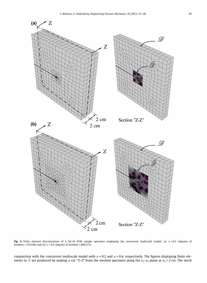
Fig. 5. Finite element discretizations of a SiC-Al FGM sample specimen employing the concurrent multiscale model: (a) j = 0.2 (degrees offreedom = 219,540) and (b) j = 0.4 (degrees of freedom = 864,573).


conjunction with the concurrent multiscale model with j = 0.2 and j = 0.4, respectively. The figures displaying finite ele-ments in D are produced by making a cut ‘‘Z–Z” from the meshed specimen along the x1–x2 plane at x3 = 2 cm. The mesh


for the concurrent model with j = 0.2 has 1064 20-noded, non-singular, quadratic brick (hexahedral) elements in D nD;25,622 10-noded, non-singular, quadratic tetrahedral elements in D nD�; and 1280 20-noded, non-singular, quadratic brickelements and 160 20-noded, quarter-point (singular), collapsed quadratic brick elements in D� along the crack front. Thenumbers of such elements are 1076, 117,412, 1280, and 160, respectively, for j = 0.4. The total degrees of freedom corre-spondingly rise from 219,540 for j = 0.2 to 864,573 for j = 0.4. The rapid increase in the number of degrees of freedomand, hence, the problem size with respect to j indicates a need for efficient stochastic multiscale analysis with a subdomainthat is as small as possible. Full 3 3 3 and four-point Gauss quadrature rules were employed for the hexahedral and tet-rahedral elements, respectively, for numerical integration. The crack faces were defined as contact surfaces due to the pres-ence of far-field out-of-plane shear stress. However, the effects of friction due to contact on modes-II and -III fracturebehaviors, if they exist, were not considered in this study.

5.2. Calculations of stress-intensity factors and reliability

The moment-modified univariate PDD method employing the concurrent multiscale fracture model was applied to cal-culate the probabilistic characteristics of SIFs and the probability of fracture initiation at three distinct crack tips, whichare marked in Fig. 4a: crack-tip A, xtip = {8,8,0}T cm; crack tip B, xtip = {8,8,2}T cm; and crack tip C, xtip = {8,8,4}T cm. Thecrack-tip subdomains ðD�Þ are 0.48 cm diameter cylinders with lengths of 0.4 cm for crack tip B and 0.2 cm for crack tipA or C, and their axes are coincident with the crack front. During Monte Carlo simulation of PDD-generated random output~ySðRÞ from Eq. (34), the material property of D� for a crack tip was selected by the following process (Fig. 4b): (1) define apoint set comprising 11 equidistant points on the portion of the crack front inside D�; (2) count the numbers of points fromthe point set falling in Dp and Dm; and (3) assign a homogeneous material property of particle (matrix) if the number ofpoints falling in Dp ðDmÞ is larger than the number of points falling in Dm ðDpÞ. However, when calculating the expansioncoefficients of �yS;pðRÞ or �yS;mðRÞ, the subdomains for crack tips A, B, and C were all assigned the same material property ofeither particle or matrix, and the remaining subdomains were assigned sample material properties, depending on the micro-structural sample. This is justified because the particle volume fraction chosen varies only in the x1 direction.

Initiation of crack growth in a three-dimensional media is a complex phenomenon because of crack-front twisting result-ing from the out-of-plane tearing mode (mode-III). There is no consensus yet on when and how a crack propagates under ageneral mixed-mode deformation because the relation between the mode-III SIF and the tendency of the crack front to twistis unknown [21]. Therefore, due to a present lack of understanding, initiation of crack propagation in a three-dimensionalconfiguration is generally evaluated at distinct crack tips on the crack front using two-dimensional mixed-mode (modes-Iand -II) criteria, where mode-III SIF and deformation are neglected [22]. In this study, the probability of fracture initiation,defined in Eq. (7), was calculated at each crack tip using yðRÞ ¼ KIc � �hðKIðRÞ;KIIðRÞÞ, where the effective SIF �hðKIðRÞ;KIIðRÞÞ isderived from the maximum circumferential stress criterion [15].

5.3. Results and discussions

Fig. 6a and b plot von Mises stress contours for two randomly selected FGM samples, generated using the concurrent mul-tiscale fracture model with j = 0.2 and j = 0.4, respectively. The effective properties required by the multiscale model werecalculated using the Mori–Tanaka approximation [16]. The overall stress responses from both samples, indicated by the con-tour patterns, are similar. However, there also exist differences in the local stress fields that may have profound implicationsin determining SIFs and eventually in reliability predictions. The results pertaining to fracture response and reliability arepresented next.

5.3.1. Moments of crack-driving forcesTable 2 lists the means and coefficients of variation of KI, KII, and KIII by the univariate PDD method employing the con-

current multiscale fracture model with two different subdomain sizes (j = 0.2 and 0.4). The statistics are tabulated for threecrack tips A, B, and C. From Table 2, the univariate PDD method yields almost the same mean values of all three SIFs at a givencrack tip when j = 0.2 and 0.4. A slight uptick in the coefficients of variation of SIFs at a given crack tip, observed when j isdoubled, is due to a larger volume of the subdomain D, which captures explicit particle location information from a largerregion around the crack front, thereby incorporating more variability into SIFs. Nonetheless, the second-moment statistics ofSIFs obtained for j = 0.2 and 0.4 are reasonably close to each other, indicating the usefulness of the concurrent multiscalemodel with the smaller subdomain for generating efficient stochastic solutions. It would be interesting to discover if thesame trend holds when comparing the sample properties or probability distributions of SIFs.

While the coefficients of variation of KI at all three crack tips are relatively uniform, KII and KIII exhibit larger coefficients ofvariation at crack tip B than at crack tips A and C. This is because the modes-II and -III SIFs at crack tip B, which is surroundedby more particles than crack tip A or C, are more sensitive to the variability of particle locations than the mode-I SIF.

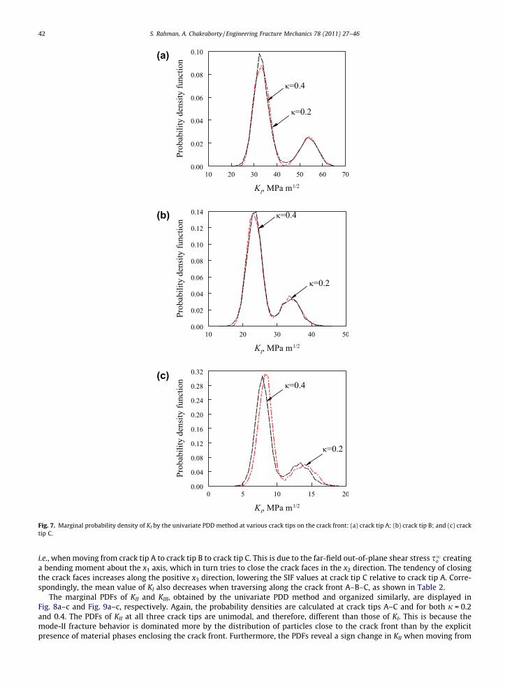
5.3.2. Probability densities of crack-driving forcesWhile the second-moment statistics are important, a more meaningful stochastic response is the PDF of a SIF. Fig. 7a–c

present the predicted marginal probability densities of KI at three crack tips A–C, respectively, obtained by the univariatePDD method and the concurrent multiscale model with j = 0.2 and 0.4. The PDFs of KI for all three crack tips reveal a bimodal

Fig. 6. von Mises stress contours for two SiC-Al FGM sample specimens employing the concurrent multiscale model: (a) j = 0.2 and (b) j = 0.4.

Table 2Second-moment statistics of SIFs by the univariate PDD method.

KI KII KIII

Crack tip Mean (MPaffiffiffiffiffimp

) COVa (%) Mean (MPaffiffiffiffiffimp

) COVa (%) Mean (MPaffiffiffiffiffimp

) COVa (%)

(a) j = 0.2A 36.788 23.147 �5.834 23.388 4.240 17.147B 25.124 18.845 1.960 52.235 5.123 28.098C 9.173 25.853 9.259 14.892 4.721 22.832

(b) j = 0.4A 38.153 24.958 �5.981 25.832 4.300 17.921B 25.936 19.982 2.009 58.648 5.371 30.086C 9.148 28.226 9.407 15.243 4.795 22.973

a The coefficient of variation (COV) is standard deviation divided by mean, when mean is not zero.


shape, where the left and right parts of the density are due to major contributions from the matrix and particle phases,respectively. The sample values of KI (horizontal co-ordinate) decrease in the positive x3 direction along the crack front,

(a)

(b)

(c)

Fig. 7. Marginal probability density of KI by the univariate PDD method at various crack tips on the crack front: (a) crack tip A; (b) crack tip B; and (c) cracktip C.


i.e., when moving from crack tip A to crack tip B to crack tip C. This is due to the far-field out-of-plane shear stress s1o creatinga bending moment about the x1 axis, which in turn tries to close the crack faces in the x2 direction. The tendency of closingthe crack faces increases along the positive x3 direction, lowering the SIF values at crack tip C relative to crack tip A. Corre-spondingly, the mean value of KI also decreases when traversing along the crack front A–B–C, as shown in Table 2.

The marginal PDFs of KII and KIII, obtained by the univariate PDD method and organized similarly, are displayed inFig. 8a–c and Fig. 9a–c, respectively. Again, the probability densities are calculated at crack tips A–C and for both j = 0.2and 0.4. The PDFs of KII at all three crack tips are unimodal, and therefore, different than those of KI. This is because themode-II fracture behavior is dominated more by the distribution of particles close to the crack front than by the explicitpresence of material phases enclosing the crack front. Furthermore, the PDFs reveal a sign change in KII when moving from

(a)

(b)

(c)

Fig. 8. Marginal probability density of KII by the univariate PDD method at various crack tips on the crack front: (a) crack tip A; (b) crack tip B; and (c) cracktip C.


crack tip A (all negative samples) to crack tip C (all positive samples), while crack tip B contains both positive and negativesample values. This is due to s1o creating a twisting moment about the x2 axis, which in turn tries to rotate the crack faces inthe x1 � x3 plane. As a result, the mean value of KII also changes sign from negative to positive values at crack tips A and C,respectively, as shown in Table 2.

In contrast, the PDFs of KIII have either unimodal or slightly bimodal shapes. The modality of the distribution of KIII de-pends on the location of a crack tip inside the three-dimensional FGM specimen. Compared with the PDFs of KI (Fig. 7b),the PDFs of KIII (Fig. 9b) at crack tip B, located at the middle of the crack front, are slightly bimodal, indicating less pro-nounced effect due to individual contributions from the matrix and particle phases. As a consequence, the bimodal shape

(a)

(b)

(c)

Fig. 9. Marginal probability density of KIII by the univariate PDD method at various crack tips on the crack front: (a) crack tip A; (b) crack tip B; and (c) cracktip C.


is lost at crack tips A and C, as they are surrounded by fewer particles than crack tip B. Therefore, the distributions of KIII atcrack tips A and C are unimodal. However, the mean values of KIII remain nearly the same along the crack front, as shown inTable 2.

The insensitivity of statistical moments of SIFs with respect to j discussed earlier also extends to the probability densitiesof SIFs, regardless of the fracture mode or crack tip examined. Indeed, the PDFs in Figs. 7–9 are practically identical when jincreases from 0.2 to 0.4. Therefore, stochastic multiscale analysis can be efficiently conducted using a smaller subdomain, atleast in this example.

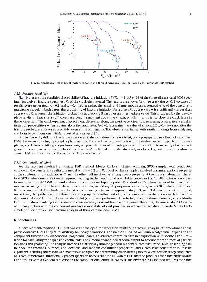
Fig. 10. Conditional probability of fracture initiation of a three-dimensional FGM specimen by the univariate PDD method.


5.3.3. Fracture reliabilityFig. 10 presents the conditional probability of fracture initiation, PF(KIc): = P[y(R) < 0], of the three-dimensional FGM spec-

imen for a given fracture toughness KIc of the crack-tip material. The results are shown for three crack tips A–C. Two cases ofresults were generated: j = 0.2 and j = 0.4, representing the small and large subdomains, respectively, of the concurrentmultiscale model. In both cases, the probability of fracture initiation for a given KIc at crack tip A is significantly larger thanat crack tip C, whereas the initiation probability at crack tip B assumes an intermediate value. This is caused by the out-of-plane far-field shear stress ðs1o Þ creating a bending moment about the x1 axis, which in turn tries to close the crack faces inthe x2 direction. The crack-opening displacement decreases along the positive x3 direction, rendering progressively smallerinitiation probabilities when moving along the crack front A–B–C. Increasing the value of j from 0.2 to 0.4 does not alter thefracture probability curves appreciably, even at the tail regions. This observation tallies with similar findings from analyzingcracks in two-dimensional FGMs reported in a prequel [9].

Due to markedly different fracture-initiation probabilities along the crack front, crack propagation in a three-dimensionalFGM, if it occurs, is a highly complex phenomenon. The crack faces following fracture initiation are not expected to remainplanar; crack front splitting and/or branching are possible. It would be intriguing to study such heterogeneity-driven crackgrowth phenomena within a stochastic framework. A multiscale probabilistic analysis of crack growth in a three-dimen-sional FGM setting is beyond the scope of the current work.

5.3.4. Computational effortFor the moment-modified univariate PDD method, Monte Carlo simulation entailing 2000 samples was conducted

employing the concurrent multiscale model with j = 0.2 and 0.4. Half of these samples involved assigning particle propertyat the subdomains of crack tips A–C, and the other half involved assigning matrix property at the same subdomains. There-fore, 2000 deterministic FEA were required, leading to the conditional probability curves in Fig. 10. All analyses were per-formed using an HP XW8400 workstation, a common desktop computer. The absolute CPU time required by concurrentmultiscale analysis of a typical deterministic sample, including all pre-processing efforts, was 270 s when j = 0.2 and925 s when j = 0.4. This leads to a full stochastic analysis times of approximately 6.3 and 21.4 days for j = 0.2 and 0.4,respectively. No probabilistic analysis using the proposed method entailing concurrent multiscale models with larger sub-domains (0.4 < j < 1) or a full microscale model (j = 1) was performed. Due to high computational demand, crude MonteCarlo simulation involving multiscale or microscale analysis is not feasible or required. Therefore, the univariate PDD meth-od in conjunction with the concurrent multiscale model developed provides an efficient alternative to crude Monte Carlosimulation for probabilistic fracture analysis of three-dimensional FGMs.

6. Conclusions

A new moment-modified PDD method was developed for stochastic multiscale fracture analysis of three-dimensional,particle-matrix FGMs subject to arbitrary boundary conditions. The method is based on Fourier-polynomial expansions ofcomponent functions by orthonormal polynomial bases, an additive control variate in conjunction with Monte Carlo simu-lation for calculating the expansion coefficients, and a moment-modified random output to account for the effects of particlelocations and geometry. The analysis involves a statistically inhomogeneous random microstructure of FGMs, describing par-ticle volume fractions, number, and locations, and random constituent properties, and a two-scale concurrent multiscalealgorithm including microscale and macroscale analyses for determining crack-driving forces. A verification study conductedon a two-dimensional functionally graded specimen reveals that the univariate PDD method produces the same crude MonteCarlo results with a five-fold reduction in the computational effort. In contrast, the bivariate PDD method requires the same


computational effort as crude Monte Carlo simulation, yielding no such computational savings when calculating tail prob-abilities equal to or larger than 10�3. Therefore, stochastic multiscale analysis can be efficiently conducted using the univar-iate method.

To illustrate the usefulness of the proposed stochastic method, a two-phase, three-dimensional, edge-cracked, function-ally graded specimen subject to mixed-mode deformation was analyzed to calculate the probabilistic characteristics ofcrack-driving forces and the probability of failure. The results demonstrate that (1) the statistical moments or probabilitydistributions of crack-driving forces and the conditional probability of fracture initiation can be efficiently generated bythe univariate method; (2) the probability distributions of mode-I and mode-II SIFs are respectively bimodal and unimodalat any crack tip but the distributions of mode-III SIFs change from unimodal to bimodal shapes, depending on the crack-tiplocation along the crack front; and (3) there exist significant variations in the probabilistic characteristics of the SIFs and thefracture-initiation probability along the crack front. Furthermore, the results are insensitive to the subdomain size from con-current multiscale analysis, which, if selected judiciously, leads to computationally efficient estimates of the probabilisticsolutions.

A stochastic analysis employing the moment-modified PDD method requires fewer deterministic FEA than crude MonteCarlo simulation. Since a single deterministic analysis of a three-dimensional configuration may come with a heavy compu-tational price tag, the newly developed decomposition method should provide an efficient alternative to crude Monte Carlosimulation for probabilistic multiscale analysis of FGMs.

Acknowledgments

The authors would like to acknowledge financial support from the US National Science Foundation under Grant No. CMS-0409463.

References

[1] Suresh S, Mortensen A. Fundamentals of functionally graded materials. London: Institute of Materials; 1998.[2] Rao BN, Rahman S. Mesh-free analysis of cracks in isotropic functionally graded materials. Eng Fract Mech 2003;70:1–27.[3] Dolbow JE, Gosz M. On the computation of mixed-mode stress intensity factors in functionally graded materials. Int J Solids Struct

2002;39(9):2557–74.[4] Kim JH, Paulino GH. Finite element evaluation of mixed-mode stress intensity factors in functionally graded materials. Int J Numer Methods Eng

2002;53(8):1903–35.[5] Walters MC, Paulino GH, Dodds Jr RH. Interaction integral procedures for 3D curved cracks including surface tractions. Eng Fract Mech

2005;72:1635–63.[6] Yildirim B, Dag S, Erdogan F. Three dimensional fracture analysis of FGM coatings under thermomechanical loading. Int J Fract 2005;132:369–95.[7] Yong H, Zhou YH. Analysis of a mode III crack problem in a functionally graded coating-substrate system with finite thickness. Int J Fract

2006;141:459–67.[8] Ferrante FJ, Graham-Brady LL. Stochastic simulation of non-gaussian/non-stationary properties in a functionally graded plate. Comput Methods Appl

Mech Eng 2005;194:1675–92.[9] Chakraborty A, Rahman S. Stochastic multiscale models for fracture analysis of functionally graded materials. Eng Fract Mech 2008;75:2062–86.

[10] Rahman S, Chakraborty A. A stochastic micromechanical model for elastic properties of functionally graded materials. Mech Mater 2007;39:548–63.[11] Quintanilla J, Torquato S. Microstructure functions for a model of statistically inhomogeneous random media. Phys Rev E 1997;55(2):1558–65.[12] Chakraborty A, Rahman S. A parametric study on probabilistic fracture of functionally graded composites by a concurrent multiscale method.

Probabilist Eng Mech 2009;24:438–51.[13] Stoyan D, Stoyan H. Fractals, random shapes and point fields: methods of geometrical statistics. New York: John Wiley & Sons, Inc.; 1994.[14] Yau JF, Wang SS, Corten HT. A mixed-mode crack analysis of isotropic solids using conservation laws of elasticity. J Appl Mech 1980;47:335–41.[15] Anderson TL. Fracture mechanics-fundamentals and applications. 3rd ed. Florida: CRC Press; 2005.[16] Mura T. Micromechanics of defects in Solids. 2nd revised ed. Dordrecht, The Netherlands: Kluwer Academic Publishers.; 1991.[17] ABAQUS, 2007. User’s guide and theoretical manual, Version 6.7, ABAQUS Inc., Providence, RI.[18] Rahman S. A polynomial dimensional decomposition for stochastic computing. Int J Numer Methods Eng 2008;76:972–93.[19] Genyuan L, Rabitz H. Ratio control variate method for efficiently determining high-dimensional model representations. J Comput Chem

2006;27:1112–8.[20] Evans M, Swartz T. Approximating integrals via Monte Carlo and deterministic methods. Oxford, New York, NY: Oxford University Press; 2000.[21] Krysl P, Belytschko T. The element-free Galerkin method for dynamic propagation of arbitrary 3D cracks. Int. J Numer Methods Eng 1999;44:767800.[22] FRANC3D, 2004. Concepts and users guide. Version 2.6, Cornell Fracture Group, Department of Civil and Environmental Engineering, Ithaca, NY.

engineering fracture mechanicsuser.engineering.uiowa.edu/~rahman/efm_multiscale3d.pdf · spatially...

Documents