symmetryS S

Article

Engineering Graphics for Thermal Assessment: 3D ThermalData Visualisation Based on Infrared Thermography, GIS and3D Point Cloud Processing Software

Daniel Antón 1,2 and José-Lázaro Amaro-Mellado 3,4,*

�����������������

Citation: Antón, D.; Amaro-Mellado,

J.-L. Engineering Graphics for

Thermal Assessment: 3D Thermal

Data Visualisation Based on Infrared

Thermography, GIS and 3D Point

Cloud Processing Software. Symmetry

2021, 13, 335. https://doi.org/

10.3390/sym13020335

Academic Editors: Sergei D. Odintsov

and José Rojas Sola

Received: 2 January 2021

Accepted: 16 February 2021

Published: 18 February 2021

Publisher’s Note: MDPI stays neutral

with regard to jurisdictional claims in

published maps and institutional affil-

iations.

Copyright: © 2021 by the authors.

Licensee MDPI, Basel, Switzerland.

This article is an open access article

distributed under the terms and

conditions of the Creative Commons

Attribution (CC BY) license (https://

creativecommons.org/licenses/by/

4.0/).

1 Research Group ‘TEP970: Innovación Tecnológica, Sistemas de Modelado 3D y Diagnosis Energética enPatrimonio y Edificación’, Departamento de Expresión Gráfica e Ingeniería en la Edificación, Escuela TécnicaSuperior de Ingeniería de Edificación, Universidad de Sevilla, 4A Reina Mercedes Avenue,41012 Seville, Spain; danton@us.es

2 The Creative and Virtual Technologies Research Laboratory, School of Architecture, Design and the BuiltEnvironment, Nottingham Trent University, 50 Shakespeare Street, Nottingham NG1 4FQ, UK

3 Departamento de Ingeniería Gráfica, Universidad de Sevilla, 41092 Seville, Spain4 Instituto Geográfico Nacional—Servicio Regional en Andalucía, 41013 Seville, Spain* Correspondence: jamaro@us.es

Abstract: Engineering graphics are present in the design stage, but also constitute a way to com-municate, analyse, and synthesise. In the Architecture-Engineering-Construction sector, graphicaldata become essential in analysing buildings and constructions throughout their lifecycles, suchas in the thermal behaviour assessment of building envelopes. Scientific research has addressedthe thermal image mapping onto three-dimensional (3D) models for visualisation and analysis.However, the 3D point cloud data creation of buildings’ thermal behaviour directly from rectifiedinfrared thermography (IRT) thermograms is yet to be investigated. Therefore, this paper develops anopen-source software graphical method to produce 3D thermal data from IRT images for temperaturevisualisation and subsequent analysis. This low-cost approach uses both a geographic informationsystem for the thermographic image rectification and the point clouds production, and 3D pointcloud processing software. The methodology has been proven useful to obtain, without perspectivedistortions, 3D thermograms even from non-radiometric raster images. The results also revealedthat non-rectangular thermograms enable over 95% of the 3D thermal data generated from IRTagainst rectangular shapes (over 85%). Finally, the 3D thermal data produced allow further thermalbehaviour assessment, including calculating the object’s heat loss and thermal transmittance fordiverse applications such as energy audits, restoration, monitoring, or product quality control.

Keywords: 3D thermal data; 3D thermograms; point cloud data; visualisation; temperature; heatloss; infrared thermography; GIS; 3D point cloud processing software; engineering graphics

1. Introduction

As a graphical expression, engineering graphics are useful for conceptual and projectrepresentation in the design stage, but also constitute a way to communicate, analyse andsynthesise [1,2]. In the Architecture-Engineering-Construction (AEC) sector, the use ofgraphical data becomes essential when dealing with the analysis of the built environment,buildings and constructions throughout their lifecycles [3]. This type of data can involve theuse of two-dimensional (2D) and three-dimensional (3D) graphics, in the form of raster andvector representations, as well as data and models based on 3D coordinates, respectively.Within this framework, several digital technologies allow the integration of additionalinformation to the graphical data, such as Geographic Information Systems (hereinafter,GIS) and Building Information Modelling (henceforth, BIM) [4]. This can be useful for theanalysis of both geometric and geographical issues, as well as buildings and constructionprocesses. In this sense, there are relevant scientific works to be highlighted dealing with the

Symmetry 2021, 13, 335. https://doi.org/10.3390/sym13020335 https://www.mdpi.com/journal/symmetry

Symmetry 2021, 13, 335 2 of 18

tools that support this research: Lerma et al. [5] implemented an architectonic GIS to analysemulti-source data, including thermal images, and rectified imagery; Previtali et al. [6] useda GIS-assisted method to improve the thermal anomalies recognition, mainly for thermalgradient assessment; Yuanrong et al. [7] designed a GIS to bring both Unmanned AerialVehicles and Terrestrial Laser Scanning data together for façade construction supervision;Chen et al. [8] used a GIS-based platform to integrate the façade data from differentsources, such as infrared thermography (hereinafter, IRT), laser scanner, or high definitiondigital cameras; and Wang et al. [9], in the frame of digital cities, studied the semanticinformation on parametrised 3D buildings’ façades by hierarchical topological graphs.In the scientific literature analysed, the information associated with the geometry of thestudied objects has been considered an attribute. Therefore, these attributes have not beenrepresented as an integral part of 3D geometric data where one of the coordinates is notgeometric. Concerning the rectification of images, it is worth highlighting the work by Yueet al. [10], who automatically rectified the building images helped by a local symmetryfeature graph. Thus, the authors matched both the original and the corrected image inorder to conduct their fusion. Finally, Soycan and Soycan [11] revised the models to achieverectified photographs for further façades analysis.

Regarding the use of 2D graphical data for building analysis, IRT is a versatile, non-destructive technology that enables the recording and visualisation of the thermal radiationemitted by the bodies. This can be used to determine energy loss in building envelopes,issues in building services, construction defects, among many others [12]. Likewise,active IRT has been proven useful to detect hidden openings or structural elements [13].The thermal image produced by IRT, called thermogram, is 2D. Still, certain proprietarysoftware for this sort of equipment such as InfReC Analyzer [14] or Fluke SmartView [15]can complement these images with 3D graphs [16,17]. Nevertheless, the 3D data that can beproduced do not represent the thermal images’ real magnitude, given the IRT survey data’sperspective distortion. Furthermore, these applications can generally be acquired togetherwith the equipment or in a complementary manner, which entails additional investment.

Scientific research has also addressed thermal image mapping onto 3D models forvisualisation and analysis. Alba et al. [18] proposed a method to texture 3D building modelsusing infrared images. Vidas et al. [19] presented a hand-held mobile system that combineda range sensor with an IRT camera to produce 3D models mapped with infrared and Red-Green-Blue colour (hereinafter, RGB) images. Wang et al. [20] developed a hybrid systemintegrating Light Detection And Ranging (LiDAR) technology and an infrared camera toproduce thermal models of building envelopes. Borrmann et al. [21] combined 3D laserscanning, IRT, and a photo camera to map 3D building façade models. Rangel et al. [22]presented an automatic approach to creating 3D thermal models by fusing IRT images andspatial data from a depth camera. Ham and Golparvar-Fard [23] proposed a 3D thermalmesh modelling method to display the as-is condition assessment of buildings. Thus, themethod permitted the visualisation of R-value distributions and potential condensationissues. Moghadam and Vidas [24] designed a hand-held 3D thermography device called”HeatWave” that combined IRT, a range sensor and a photo camera to create 3D modelswith augmented temperature and visible information of the objects. Moghadam [25] alsopresented a hand-held 3D device for medical thermography to simultaneously show both3D thermal and colour information to facilitate diagnosis. Matsumoto et al. [26] developeda hand-held system based on IRT and an RGB-D (RGB depth sensor) camera for 3D modeland temperature change visualisation from arbitrary viewpoints via augmented reality.Nakagawa et al. [27] established a system combining IRT and an RGB-D camera for scene3D reconstruction; later, the authors applied the Viewpoint Generative Learning methodto the RGB 3D model to display the difference between the temperature of random sceneviewpoints and known camera poses. Natephra et al. [28] integrated thermographic imagesalong with air temperature and relative humidity values into BIM to create 4D models ofthe performance of existing building envelopes. Finally, Landmann et al. [29] presented ahigh-speed system based on a structured-light sensor and an infrared camera to measure

Symmetry 2021, 13, 335 3 of 18

3D geometry and the fast-moving objects’ temperature. The reviewed scientific literaturecontinues to address the problem of representing the thermal behaviour of objects byassociating thermal attributes (images and RGB values) to purely geometric 3D data, withspatial coordinates.

In view of the above, the creation of 3D point cloud data of buildings’ thermal be-haviour for visualisation and analysis directly from rectified IRT thermograms is yet to beinvestigated. Given this knowledge gap, the aim of this paper is to provide an open-sourcesoftware graphical method to produce three-dimensional thermal data from the infraredthermovision technique. It should be noted that, with the emergence and development ofopen data and open-source software, this can be addressed free of charge or at low cost.Consequently, the low-cost approach developed in this research (excluding the cost of IRTequipment), applies both thermographic image rectification in GIS and 3D point cloud datamanagement. It has been proven useful to achieve, without perspective distortions, the 3Dvisualisation of the temperature of the objects surveyed. Thus, the methodology enablesadditional analysis of their thermal behaviour, which could not have been carried out if thethermal information (attribute) had not been converted into a third geometrical variable(coordinate) in the 3D thermal data set produced. The proposed method is tested in twocase studies: (1) a quasi-symmetrical building façade sector, and (2) a non-symmetricalfaçade sector. This research also studied the impact of choosing between rectangular andnon-rectangular 3D thermograms after the image rectification in GIS in terms of thermaldata loss.

The rest of the paper is structured as follows: (Section 2) the methodology is de-scribed and subdivided into stages corresponding to each technology used in this research;(Section 3) the results of the two cases studied are presented; and (Section 4) the resultsof this research and its limitations are discussed; likewise, conclusions and future workare provided.

2. Methodology

As mentioned above, this research is based on the combination of IRT and GIS, plusthe treatment and management of 3D point cloud data for analysis. Thus, each technologyconstitutes a stage in the suggested methodology:

2.1. Thermal Imaging

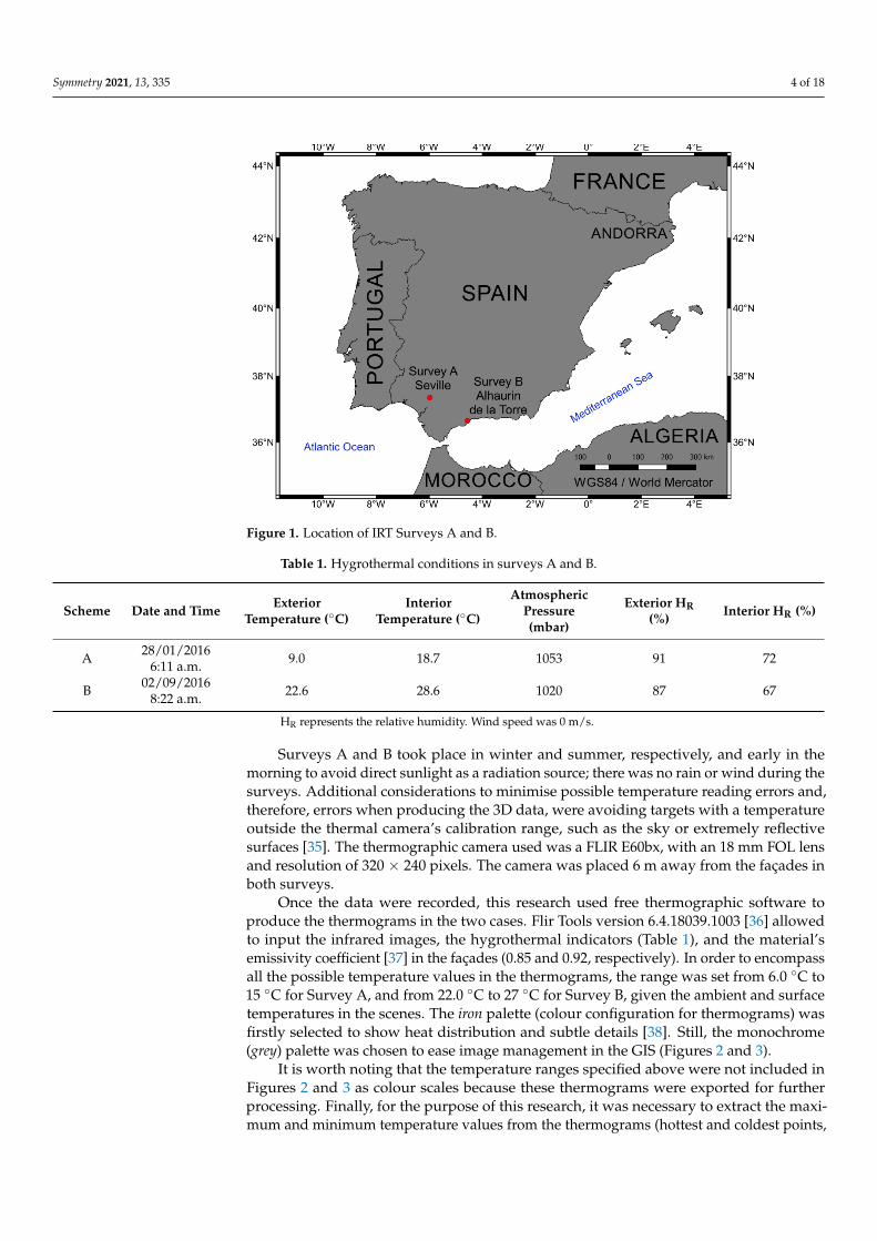
The first stage of the proposed method is to record the façade building components’temperature via IRT. In this research, this was carried out in two surveys in Andalusia,Spain (Figure 1): Survey A, in the south of the city of Seville (inland Mediterranean climate),and Survey B, in Alhaurin de la Torre, near Malaga (coastal Mediterranean climate).

The IRT surveys focused on the thermal bridge caused by the buildings’ reinforcedconcrete structure due to the lack of thermal insulation between the pillar and slabs and(1) the rendered brick façade (Survey A, a quasi-symmetrical sector), and (2) the vibratedconcrete rough block façade (Survey B, a non-symmetrical sector).

The recording of the surface temperature in the IRT surveys is affected by changesin the directional emissivity due to different viewing angles (between the direction of thecamera and the object’s emission direction) higher than 40◦ [30–34]. Moreover, the cameraoperators themselves constitute a source of emissions that must be taken into accountby avoiding the perpendicularity between the camera direction and the object. Theseaspects were considered in the surveys of this research so that both procedural errorsand environmental radiant sources, respectively, were minimised in the recording of thefaçades’ surface temperatures.

Besides, the weather conditions were recorded 24 h before the surveys using a portableweather station with sensors inside and outside the buildings. The hygrothermal indicators,input in both the camera settings and the thermographic software along with the material’semissivity to produce the thermograms (graphical output of the IRT surveys), are gatheredin Table 1.

Symmetry 2021, 13, 335 4 of 18Symmetry 2021, 13, 335 4 of 20

Figure 1. Location of IRT Surveys A and B.

The IRT surveys focused on the thermal bridge caused by the buildings’ reinforced concrete structure due to the lack of thermal insulation between the pillar and slabs and (1) the rendered brick façade (Survey A, a quasi-symmetrical sector), and (2) the vibrated concrete rough block façade (Survey B, a non-symmetrical sector).

The recording of the surface temperature in the IRT surveys is affected by changes in the directional emissivity due to different viewing angles (between the direction of the camera and the object’s emission direction) higher than 40° [30–34]. Moreover, the camera operators themselves constitute a source of emissions that must be taken into account by avoiding the perpendicularity between the camera direction and the object. These aspects were considered in the surveys of this research so that both procedural errors and environmental radiant sources, respectively, were minimised in the recording of the façades’ surface temperatures.

Besides, the weather conditions were recorded 24 h before the surveys using a portable weather station with sensors inside and outside the buildings. The hygrothermal indicators, input in both the camera settings and the thermographic software along with the material’s emissivity to produce the thermograms (graphical output of the IRT surveys), are gathered in Table 1.

Table 1. Hygrothermal conditions in surveys A and B.

Scheme Date and Time Exterior Temperature (°C)

Interior Temperature (°C)

Atmospheric Pressure (mbar)

Exterior HR (%)

Interior HR (%)

A 28/01/2016 6:11 a.m. 9.0 18.7 1053 91 72

B 02/09/2016 8:22

a.m. 22.6 28.6 1020 87 67

HR represents the relative humidity. Wind speed was 0 m/s.

Surveys A and B took place in winter and summer, respectively, and early in the morning to avoid direct sunlight as a radiation source; there was no rain or wind during the surveys. Additional considerations to minimise possible temperature reading errors and, therefore, errors when producing the 3D data, were avoiding targets with a

Figure 1. Location of IRT Surveys A and B.

Table 1. Hygrothermal conditions in surveys A and B.

Scheme Date and Time ExteriorTemperature (◦C)

InteriorTemperature (◦C)

AtmosphericPressure(mbar)

Exterior HR(%) Interior HR (%)

A 28/01/20166:11 a.m. 9.0 18.7 1053 91 72

B 02/09/20168:22 a.m. 22.6 28.6 1020 87 67

HR represents the relative humidity. Wind speed was 0 m/s.

Surveys A and B took place in winter and summer, respectively, and early in themorning to avoid direct sunlight as a radiation source; there was no rain or wind during thesurveys. Additional considerations to minimise possible temperature reading errors and,therefore, errors when producing the 3D data, were avoiding targets with a temperatureoutside the thermal camera’s calibration range, such as the sky or extremely reflectivesurfaces [35]. The thermographic camera used was a FLIR E60bx, with an 18 mm FOL lensand resolution of 320 × 240 pixels. The camera was placed 6 m away from the façades inboth surveys.

Once the data were recorded, this research used free thermographic software toproduce the thermograms in the two cases. Flir Tools version 6.4.18039.1003 [36] allowedto input the infrared images, the hygrothermal indicators (Table 1), and the material’semissivity coefficient [37] in the façades (0.85 and 0.92, respectively). In order to encompassall the possible temperature values in the thermograms, the range was set from 6.0 ◦C to15 ◦C for Survey A, and from 22.0 ◦C to 27 ◦C for Survey B, given the ambient and surfacetemperatures in the scenes. The iron palette (colour configuration for thermograms) wasfirstly selected to show heat distribution and subtle details [38]. Still, the monochrome(grey) palette was chosen to ease image management in the GIS (Figures 2 and 3).

It is worth noting that the temperature ranges specified above were not included inFigures 2 and 3 as colour scales because these thermograms were exported for furtherprocessing. Finally, for the purpose of this research, it was necessary to extract the maxi-mum and minimum temperature values from the thermograms (hottest and coldest points,

Symmetry 2021, 13, 335 5 of 18

respectively). Thus, the extent of the third dimension (of the 3D thermal data) could benext obtained from the temperature range using GIS.

Symmetry 2021, 13, 335 5 of 20

temperature outside the thermal camera’s calibration range, such as the sky or extremely reflective surfaces [35]. The thermographic camera used was a FLIR E60bx, with an 18 mm FOL lens and resolution of 320 × 240 pixels. The camera was placed 6 m away from the façades in both surveys.

Once the data were recorded, this research used free thermographic software to produce the thermograms in the two cases. Flir Tools version 6.4.18039.1003 [36] allowed to input the infrared images, the hygrothermal indicators (Table 1), and the material’s emissivity coefficient [37] in the façades (0.85 and 0.92, respectively). In order to encompass all the possible temperature values in the thermograms, the range was set from 6.0 °C to 15 °C for Survey A, and from 22.0 °C to 27 °C for Survey B, given the ambient and surface temperatures in the scenes. The iron palette (colour configuration for thermograms) was firstly selected to show heat distribution and subtle details [38]. Still, the monochrome (grey) palette was chosen to ease image management in the GIS (Figures 2 and 3).

(a) (b)

Figure 2. Thermograms of Survey A for GIS processing: (a) Iron palette; (b) Grey (monochrome) palette.

(a) (b)

Figure 3. Thermograms of Survey B for GIS processing: (a) Iron palette; (b) Grey (monochrome) palette.

It is worth noting that the temperature ranges specified above were not included in Figures 2 and 3 as colour scales because these thermograms were exported for further processing. Finally, for the purpose of this research, it was necessary to extract the maximum and minimum temperature values from the thermograms (hottest and coldest

Figure 2. Thermograms of Survey A for GIS processing: (a) Iron palette; (b) Grey (monochrome) palette.

Symmetry 2021, 13, 335 5 of 20

temperature outside the thermal camera’s calibration range, such as the sky or extremely reflective surfaces [35]. The thermographic camera used was a FLIR E60bx, with an 18 mm FOL lens and resolution of 320 × 240 pixels. The camera was placed 6 m away from the façades in both surveys.

Once the data were recorded, this research used free thermographic software to produce the thermograms in the two cases. Flir Tools version 6.4.18039.1003 [36] allowed to input the infrared images, the hygrothermal indicators (Table 1), and the material’s emissivity coefficient [37] in the façades (0.85 and 0.92, respectively). In order to encompass all the possible temperature values in the thermograms, the range was set from 6.0 °C to 15 °C for Survey A, and from 22.0 °C to 27 °C for Survey B, given the ambient and surface temperatures in the scenes. The iron palette (colour configuration for thermograms) was firstly selected to show heat distribution and subtle details [38]. Still, the monochrome (grey) palette was chosen to ease image management in the GIS (Figures 2 and 3).

(a) (b)

Figure 2. Thermograms of Survey A for GIS processing: (a) Iron palette; (b) Grey (monochrome) palette.

(a) (b)

Figure 3. Thermograms of Survey B for GIS processing: (a) Iron palette; (b) Grey (monochrome) palette.

It is worth noting that the temperature ranges specified above were not included in Figures 2 and 3 as colour scales because these thermograms were exported for further processing. Finally, for the purpose of this research, it was necessary to extract the maximum and minimum temperature values from the thermograms (hottest and coldest

Figure 3. Thermograms of Survey B for GIS processing: (a) Iron palette; (b) Grey (monochrome) palette.

2.2. GIS-Based Image Management

GIS are tools that facilitate the handling of geographic information rigorously ineach process phase, such as data entry, storage, management, integration, edition, orvisualisation. Their most common use is in work on the horizontal plane, as shown inthe recent literature, such as [39–43]. By contrast, there are fewer cases for working withelevation [5,8], even if this only involves a change in coordinate axes.

In this work, a GIS has been used to carry out the thermogram’s geometric rectificationand assign temperatures to the rectified image. QGIS v3.8.2 software [44] was used inthis research.

In both surveys, it has been assumed that the area of interest is contained in a plane.Thus, the relief (depth) of the façade is not deemed. For this reason, instead of an orthorec-tification, only a 2D homography, or projective transformation is required. Here, eightparameters are considered to conduct perspective removal. This planar homography aimsat transforming one plane into another, and can be expressed as [11]: x

y1

= H

XY1

=

h11 h12 h13h21 h22 h23h31 h32 h33

XY1

(1)

Symmetry 2021, 13, 335 6 of 18

Although the matrix presents nine parameters, the transformation poses eight degreesof freedom because the values are usually normalised, considering h33 = 1 (Figure 4). Theeight parameters can be easily calculated from four pairs of points, both identified in thetwo spaces.

Symmetry 2021, 13, 335 6 of 20

points, respectively). Thus, the extent of the third dimension (of the 3D thermal data) could be next obtained from the temperature range using GIS.

2.2. GIS-Based Image ManagementGIS are tools that facilitate the handling of geographic information rigorously in each

process phase, such as data entry, storage, management, integration, edition, or visualisation. Their most common use is in work on the horizontal plane, as shown in the recent literature, such as [39–43]. By contrast, there are fewer cases for working with elevation [5,8], even if this only involves a change in coordinate axes.

In this work, a GIS has been used to carry out the thermogram’s geometric rectification and assign temperatures to the rectified image. QGIS v3.8.2 software [44] wasused in this research.

In both surveys, it has been assumed that the area of interest is contained in a plane. Thus, the relief (depth) of the façade is not deemed. For this reason, instead of an orthorectification, only a 2D homography, or projective transformation is required. Here, eight parameters are considered to conduct perspective removal. This planar homography aims at transforming one plane into another, and can be expressed as [11]: 𝑥𝑦1 = 𝐻 𝑋𝑌1 = ℎ ℎ ℎℎ ℎ ℎ ℎ ℎ ℎ

𝑋𝑌1 (1)

Although the matrix presents nine parameters, the transformation poses eight degrees of freedom because the values are usually normalised, considering h33 = 1 (Figure 4). The eight parameters can be easily calculated from four pairs of points, both identified in the two spaces.

Figure 4. Homographic transformation to remove the perspective distortion.

First, the geometrical measurement framework has to be defined. In this case, since this research presents a low-cost method, it has been preferred not to use classic topographical methods but a plumb, a spirit level, and a measuring tape. • For Survey A, the façade itself served as a reference:

- Y-axis: the (left) vertical limit of the façade; - X-axis: a mortar joint; a spirit level was used to check its horizontality.

• For Survey B: - Y-axis: a vertical joint, after checking with a plumb that its extension coincides

with another of the lower joints; - X-axis: a horizontal mortar joint, whose horizontality has been verified using a

spirit level. Contrary to conventional topography, the distance measurements have been

established a posteriori. To this end, it has been checked that the four points that will

Figure 4. Homographic transformation to remove the perspective distortion.

First, the geometrical measurement framework has to be defined. In this case, since thisresearch presents a low-cost method, it has been preferred not to use classic topographicalmethods but a plumb, a spirit level, and a measuring tape.

• For Survey A, the façade itself served as a reference:

- Y-axis: the (left) vertical limit of the façade;- X-axis: a mortar joint; a spirit level was used to check its horizontality.

• For Survey B:

- Y-axis: a vertical joint, after checking with a plumb that its extension coincideswith another of the lower joints;

- X-axis: a horizontal mortar joint, whose horizontality has been verified using aspirit level.

Contrary to conventional topography, the distance measurements have been estab-lished a posteriori. To this end, it has been checked that the four points that will define thegeometric frame are identifiable in the thermogram, using the diagonal as a verification.The measurements (and the axes) taken are displayed in Figure 5 on each thermogram.

Symmetry 2021, 13, 335 7 of 20

define the geometric frame are identifiable in the thermogram, using the diagonal as a verification. The measurements (and the axes) taken are displayed in Figure 5 on each thermogram.

(a) (b)

Figure 5. Measurements taken for perspective correction: (a) Survey A; (b) Survey B.

Along with the geometrical 2D-homography, a radiometric conversion must be undertaken. Thereby, a digital number (DN) value must be assigned to each pixel of the resulting image. Besides, a bicubic interpolation has been chosen to conduct the resampling process.

After obtaining an image with the rectified geometry and the corresponding DN, the next step is for each pixel’s DN to correspond to the thermogram’s temperature. In both surveys, each thermogram was encoded on 8 bits, i.e., 256 values, as radiometric resolution. For the DN value to correlate with the temperature, a linear normalisation formula must be applied: 𝐷𝑁 = 𝑎 × 𝐷𝑁 + 𝑏 (2)

where a is the slope, that is related to the rectified image’s thermal sensitivity, and b is the intercept, the minimum temperature value. From the temperature values of each case, the calculated parameters are shown in Table 2. Thus, it can be concluded that the thermal resolution for the rectified image for Survey B is approximately three times better than that for Survey A:

Table 2. Extreme temperatures and conversion parameters for each survey.

Scheme Tmin (°C) Tmax (°C) DNmin DNmax a b A 6.9 14.0 0 255 0.02784 6.9 B 23.0 25.4 0 255 0.00941 23.0

For each pixel in the new image, the DN coincides with the temperature recorded. The image border has a dark background, which corresponds to the absence of data. This fact is inherent in any “photograph”. Due to the inclination, there will be points on the resampled image that lack information. The tilt is determined by the commitment to obtain an image covering as much spatial coverage as possible without a significant loss of geometric resolution (pixel size on the facade). This matter is especially relevant since the thermographic camera used only has 320 × 240 pixels.

Theoretically, a rectangular region of interest (hereinafter, ROI), in which all the pixels would have their temperature recorded, is more appropriate in terms of graphic language. However, this is not always suited, as information not included in the rectangle

Figure 5. Measurements taken for perspective correction: (a) Survey A; (b) Survey B.

Along with the geometrical 2D-homography, a radiometric conversion must be under-taken. Thereby, a digital number (DN) value must be assigned to each pixel of the resultingimage. Besides, a bicubic interpolation has been chosen to conduct the resampling process.

After obtaining an image with the rectified geometry and the corresponding DN, thenext step is for each pixel’s DN to correspond to the thermogram’s temperature. In both

Symmetry 2021, 13, 335 7 of 18

surveys, each thermogram was encoded on 8 bits, i.e., 256 values, as radiometric resolution.For the DN value to correlate with the temperature, a linear normalisation formula mustbe applied:

DNtemp = a× DN + b (2)

where a is the slope, that is related to the rectified image’s thermal sensitivity, and b is theintercept, the minimum temperature value. From the temperature values of each case, thecalculated parameters are shown in Table 2. Thus, it can be concluded that the thermalresolution for the rectified image for Survey B is approximately three times better than thatfor Survey A:

Table 2. Extreme temperatures and conversion parameters for each survey.

Scheme Tmin (◦C) Tmax (◦C) DNmin DNmax a b

A 6.9 14.0 0 255 0.02784 6.9B 23.0 25.4 0 255 0.00941 23.0

For each pixel in the new image, the DN coincides with the temperature recorded.The image border has a dark background, which corresponds to the absence of data. Thisfact is inherent in any “photograph”. Due to the inclination, there will be points on theresampled image that lack information. The tilt is determined by the commitment toobtain an image covering as much spatial coverage as possible without a significant loss ofgeometric resolution (pixel size on the facade). This matter is especially relevant since thethermographic camera used only has 320 × 240 pixels.

Theoretically, a rectangular region of interest (hereinafter, ROI), in which all the pixelswould have their temperature recorded, is more appropriate in terms of graphic language.However, this is not always suited, as information not included in the rectangle can be lost.This happens in survey B, where the slab thermal bridge above the rectangle has furthertemperature data.

Operating in a GIS environment allows fitting as much work area as possible bydefining an area of interest that is not rectangular. This area has been used as a mask whenexporting the data for the following processes.

2.3. 3D Point Cloud Data Treatment

For the purpose of this work, the three-dimensional data produced in the GIS platformneed certain transformations to constitute the final 3D thermal data. This was carriedout in CloudCompare v2.91 for 64-bit Microsoft Windows [45], although there are otheropen-source applications such as MeshLab [46] that can be used.

Firstly, the data were imported into the programme as the XYZ file created in theprevious stage in GIS.

Next, a height ramp [47] or a height map of the 3D point set was generated to enhancethe visualisation and readability of the 3D thermal data produced. This was performedusing a monochrome linear gradient, 8-bit encoding (black for the lowest temperature,white for the highest), and a direction (Z-axis). The red, green and blue values of the RGBcolours applied were therefore automatically associated with the coordinates of each pointin the 3D point cloud.

It should be also noted that the temperature range of the thermograms determines thedistribution of the points in the 3D thermal data. In other words, given that the third coor-dinate (Z) is represented in the three-dimensional thermal data as its temperature values(◦C), it may be that these values are actually higher than the XY coordinates (dimensions ofthe object studied). As a result, interpretating the 3D point cloud’s proportions may not beeasy. Therefore, to reduce the ”temperature-value/X-Y-dimensions” ratio, a scale factor of0.10 was applied to the Z-axis (temperatures). Thus, a more representative 3D point set ofthe thermal behaviour of the façade was obtained.

Symmetry 2021, 13, 335 8 of 18

Further management of the 3D thermal data makes it possible to gather useful informa-tion such as those façade sectors at a similar temperature. This can be carried out by creatingpoint cloud contours by elevation (Z coordinate) thresholds. Considering that the Z-axisrepresents the temperature, these contours or 2D isolines—points with the same heightor Z coordinate as in topographic maps—represent the thermogram isotherms—imageregions within the same temperature range. The ”Rasterize” plugin [48] in CloudComparehelps create these isotherms by setting the gap (step) between the lines in the ”Contourplot” sub-tool, according to the temperature range of the façades. In this case, Survey Bwas considered to show the isotherms creation, conducted every 0.25◦C from 23.25◦C to25.00◦C. The contours can be exported in different file formats such as the broadly-usedDXF. The results of the isotherm creation process are presented in the following section.

Finally, the ‘Rasterize’ plugin enables the creation of meshes from point clouds throughthe Delaunay 2.5D triangulation algorithm in the XY plane [49]. This is a suitable methodto create 3D meshes from rather flat point clouds oriented to the Z-axis as in this research.

3. Results

In line with the methodology, this section is divided into the different technologiesand processes considered in this research, particularly GIS and 3D point cloud data. Thereason for not including the IRT results is that the thermograms from Surveys A and B arethe method’s data source. Besides, they are already presented in Section 2.1 as an inherentpart of the IRT surveys.

3.1. Image Management in GIS

The perspective correction was performed as per Section 2.3 to produce a rectangularROI for the thermogram in Survey A. Nevertheless, given the slab’s thermal bridge inSurvey B, the ROI selected included the thermal data of that area in the 3D point cloud(Figure 6).

Symmetry 2021, 13, 335 9 of 20

Survey B, the ROI selected included the thermal data of that area in the 3D point cloud (Figure 6).

(a) (b)

Figure 6. Rectified thermograms from Survey B: (a) Rectangular image; (b) Better-fitted image.

In order to avoid duplication of figures, the rectified thermogram from Survey A will be presented in the following section as 3D thermal data.

3.2. 3D Thermal Data Following Section 2.3, an 8-bit monochrome linear gradient height ramp was applied

to the point sets, and a factor of 0.10 was next used to scale the Z-axis (temperature) to obtain a more representative 3D thermal data set (better point distribution) (Figures 7 and 8).

(a) (b)

Figure 7. Isometric view of the 3D thermal data from Survey A: (a) original height-map 3D thermal data; (b) scaled height-map 3D thermal data.

Figure 6. Rectified thermograms from Survey B: (a) Rectangular image; (b) Better-fitted image.

In order to avoid duplication of figures, the rectified thermogram from Survey A willbe presented in the following section as 3D thermal data.

3.2. 3D Thermal Data

Following Section 2.3, an 8-bit monochrome linear gradient height ramp was appliedto the point sets, and a factor of 0.10 was next used to scale the Z-axis (temperature) to obtaina more representative 3D thermal data set (better point distribution) (Figures 7 and 8).

Symmetry 2021, 13, 335 9 of 18

Symmetry 2021, 13, 335 9 of 20

Survey B, the ROI selected included the thermal data of that area in the 3D point cloud (Figure 6).

(a) (b)

Figure 6. Rectified thermograms from Survey B: (a) Rectangular image; (b) Better-fitted image.

In order to avoid duplication of figures, the rectified thermogram from Survey A will be presented in the following section as 3D thermal data.

3.2. 3D Thermal Data Following Section 2.3, an 8-bit monochrome linear gradient height ramp was applied

to the point sets, and a factor of 0.10 was next used to scale the Z-axis (temperature) to obtain a more representative 3D thermal data set (better point distribution) (Figures 7 and 8).

(a) (b)

Figure 7. Isometric view of the 3D thermal data from Survey A: (a) original height-map 3D thermal data; (b) scaled height-map 3D thermal data. Figure 7. Isometric view of the 3D thermal data from Survey A: (a) original height-map 3D thermal

data; (b) scaled height-map 3D thermal data.

Symmetry 2021, 13, 335 10 of 20

(a) (b)

Figure 8. Isometric view of the 3D thermal data from Survey B: (a) original height-map 3D thermal data; (b) scaled height-map 3D thermal data.

Also, the top-view visualisation of the 3D height ramp produced shows the (rectified) original thermogram obtained using GIS as per Section 2.2. In turn, this helps to identify in 2D the most significant façade components or parts with the highest temperature and, consequently, those with the greatest energy loss (Figures 9 and 10).

Figure 9. Top view of the 3D thermal data from Survey A.

Figure 8. Isometric view of the 3D thermal data from Survey B: (a) original height-map 3D thermaldata; (b) scaled height-map 3D thermal data.

Also, the top-view visualisation of the 3D height ramp produced shows the (rectified)original thermogram obtained using GIS as per Section 2.2. In turn, this helps to identifyin 2D the most significant façade components or parts with the highest temperature and,consequently, those with the greatest energy loss (Figures 9 and 10).

Symmetry 2021, 13, 335 10 of 20

(a) (b)

Figure 8. Isometric view of the 3D thermal data from Survey B: (a) original height-map 3D thermal data; (b) scaled height-map 3D thermal data.

Also, the top-view visualisation of the 3D height ramp produced shows the (rectified) original thermogram obtained using GIS as per Section 2.2. In turn, this helps to identify in 2D the most significant façade components or parts with the highest temperature and, consequently, those with the greatest energy loss (Figures 9 and 10).

Figure 9. Top view of the 3D thermal data from Survey A. Figure 9. Top view of the 3D thermal data from Survey A.

Symmetry 2021, 13, 335 10 of 18Symmetry 2021, 13, 335 11 of 20

Figure 10. Top view of the 3D thermal data from Survey B.

It should be noted that, when visualised in top view, the 3D thermogram from Survey B is not oblong as the one from Survey A because of the perspective correction into a rectangular shape. This is because the thermogram rectified in the GIS for Survey B includes the cropped area which was discarded after the image rectification as in Survey A. As a result, more radiometric data can be obtained by following the approach for Survey B.

3.2.1. Quantitative Analysis Concerning the quantitative results that can be obtained from enquiring the 3D

thermal data, diverse information about the thermal behaviour of the case studies can be obtained: • The proposed method produced 68,461 points from Survey A, whereas the 3D

thermogram from Survey B contains 73,085 points (non-rectangular ROI), and 65,572 points (rectangular ROI);

• In Survey A, the temperature values (Z coordinate) enable to gather relevant information of the façade’s thermal behaviour. The lowest temperature is 7.011 °C, and the highest is 13.722 °C (6.710 °C temperature range). The average temperature of the façade is 9.895 °C, and the standard deviation is 1.165 °C.

• In Survey B, the focus is on the non-rectangular thermogram, given the larger amount of thermal data produced against the rectangular ROI approach. The lowest temperature is 23.169 °C, and the highest is 25.164 °C (1.995 °C temperature range). The average temperature is 24.021 °C, and the standard deviation is 0.410 °C. The distribution of temperatures is shown in the histograms for each survey in Figures

11 and 12:

Figure 10. Top view of the 3D thermal data from Survey B.

It should be noted that, when visualised in top view, the 3D thermogram from SurveyB is not oblong as the one from Survey A because of the perspective correction into arectangular shape. This is because the thermogram rectified in the GIS for Survey Bincludes the cropped area which was discarded after the image rectification as in Survey A.As a result, more radiometric data can be obtained by following the approach for Survey B.

3.2.1. Quantitative Analysis

Concerning the quantitative results that can be obtained from enquiring the 3D thermaldata, diverse information about the thermal behaviour of the case studies can be obtained:

• The proposed method produced 68,461 points from Survey A, whereas the 3D thermo-gram from Survey B contains 73,085 points (non-rectangular ROI), and 65,572 points(rectangular ROI);

• In Survey A, the temperature values (Z coordinate) enable to gather relevant infor-mation of the façade’s thermal behaviour. The lowest temperature is 7.011 ◦C, andthe highest is 13.722 ◦C (6.710 ◦C temperature range). The average temperature of thefaçade is 9.895 ◦C, and the standard deviation is 1.165 ◦C.

• In Survey B, the focus is on the non-rectangular thermogram, given the larger amountof thermal data produced against the rectangular ROI approach. The lowest temper-ature is 23.169 ◦C, and the highest is 25.164 ◦C (1.995 ◦C temperature range). Theaverage temperature is 24.021 ◦C, and the standard deviation is 0.410 ◦C.

The distribution of temperatures is shown in the histograms for each survey inFigures 11 and 12:

Symmetry 2021, 13, 335 11 of 18Symmetry 2021, 13, 335 12 of 20

Figure 11. 3D thermal data distribution in Survey A.

Figure 12. 3D thermal data distribution in Survey B.

In view of Figures 11 and 12, the most frequent temperature values are between 10.0 and 11.0 °C in Survey A, and between 23.5 and 24.5 °C in Survey B, approximately ―a difference of 1 °C in both cases.

3.2.2. From 3D Point Cloud Thermal Data to (2+1)D Isotherms and 3D Meshes In order to provide additional quantitative and qualitative data from the 3D thermal

point clouds, the ”Rasterize” plugin in CloudCompare [48] allows for creating isotherms and a 3D mesh from a point cloud. This was carried out for Survey B. The ‘Contour plot’ sub-tool was used to create planar isotherms, graded in the Z-axis (temperature) every 0.25 °C from 23.25 °C to 25.00 °C, given the temperature values in the case study (Figure 13).

Figure 11. 3D thermal data distribution in Survey A.

Symmetry 2021, 13, 335 12 of 20

Figure 11. 3D thermal data distribution in Survey A.

Figure 12. 3D thermal data distribution in Survey B.

In view of Figures 11 and 12, the most frequent temperature values are between 10.0 and 11.0 °C in Survey A, and between 23.5 and 24.5 °C in Survey B, approximately ―a difference of 1 °C in both cases.

3.2.2. From 3D Point Cloud Thermal Data to (2+1)D Isotherms and 3D Meshes In order to provide additional quantitative and qualitative data from the 3D thermal

point clouds, the ”Rasterize” plugin in CloudCompare [48] allows for creating isotherms and a 3D mesh from a point cloud. This was carried out for Survey B. The ‘Contour plot’ sub-tool was used to create planar isotherms, graded in the Z-axis (temperature) every 0.25 °C from 23.25 °C to 25.00 °C, given the temperature values in the case study (Figure 13).

Figure 12. 3D thermal data distribution in Survey B.

In view of Figures 11 and 12, the most frequent temperature values are between 10.0and 11.0 ◦C in Survey A, and between 23.5 and 24.5 ◦C in Survey B, approximately—adifference of 1 ◦C in both cases.

3.2.2. From 3D Point Cloud Thermal Data to (2+1)D Isotherms and 3D Meshes

In order to provide additional quantitative and qualitative data from the 3D thermalpoint clouds, the ”Rasterize” plugin in CloudCompare [48] allows for creating isothermsand a 3D mesh from a point cloud. This was carried out for Survey B. The ‘Contourplot’ sub-tool was used to create planar isotherms, graded in the Z-axis (temperature)every 0.25 ◦C from 23.25 ◦C to 25.00 ◦C, given the temperature values in the case study(Figure 13).

Besides, the point cloud was discretised in order to create the 3D mesh displayed inthe different modes in Figure 14.

Symmetry 2021, 13, 335 12 of 18Symmetry 2021, 13, 335 13 of 20

Figure 13. Top view of the isotherms from the 3D thermal data in Survey B.

Besides, the point cloud was discretised in order to create the 3D mesh displayed in the different modes in Figure 14.

Figure 14. Isometric view of the 3D thermal data from Survey B: (left) Isotherms; (centre) Wireframe mesh and isotherms; (right) Solid mesh.

The mesh produced contains 145,996 faces, approximately twice the number of vertices, as seen in Antón et al. [50]. In order to verify the accuracy of the meshing process [51], it is worth computing the distance between the scaled height-ramp cloud and the ”Rasterize”-tool mesh. This was conducted using the Multiscale Model to Model Cloud Comparison (M3C2) algorithm by Lague et al. [52] to measure the orthogonal distance between the mesh vertexes and the original 3D thermal data (the reference in the

Figure 13. Top view of the isotherms from the 3D thermal data in Survey B.

Symmetry 2021, 13, 335 13 of 20

Figure 13. Top view of the isotherms from the 3D thermal data in Survey B.

Besides, the point cloud was discretised in order to create the 3D mesh displayed in the different modes in Figure 14.

Figure 14. Isometric view of the 3D thermal data from Survey B: (left) Isotherms; (centre) Wireframe mesh and isotherms; (right) Solid mesh.

The mesh produced contains 145,996 faces, approximately twice the number of vertices, as seen in Antón et al. [50]. In order to verify the accuracy of the meshing process [51], it is worth computing the distance between the scaled height-ramp cloud and the ”Rasterize”-tool mesh. This was conducted using the Multiscale Model to Model Cloud Comparison (M3C2) algorithm by Lague et al. [52] to measure the orthogonal distance between the mesh vertexes and the original 3D thermal data (the reference in the

Figure 14. Isometric view of the 3D thermal data from Survey B: (left) Isotherms; (centre) Wireframe mesh and isotherms;(right) Solid mesh.

The mesh produced contains 145,996 faces, approximately twice the number of vertices,as seen in Antón et al. [50]. In order to verify the accuracy of the meshing process [51], it isworth computing the distance between the scaled height-ramp cloud and the ”Rasterize”-tool mesh. This was conducted using the Multiscale Model to Model Cloud Comparison(M3C2) algorithm by Lague et al. [52] to measure the orthogonal distance between themesh vertexes and the original 3D thermal data (the reference in the comparison). Thereason for choosing the M3C2 method is that, according to its authors, it performs well incomparing point cloud data, even in complex 3D environments. Likewise, it is implementedin CloudCompare as a plugin [53], which eases the process given that there is no needto use different software to compute the point deviation. In this operation, the point

Symmetry 2021, 13, 335 13 of 18

normals (normal vectors of points) [54] of the original cloud (normals oriented to theZ-axis direction) were used to compute the distances. The mean distance was 0.00038 m,and the standard deviation was 0.000143 m; these data reveal the remarkable similaritybetween the point sets, given the negligible distance between homologous points. In fact,the comparison revealed that most of the points (70,825, which constitute 96.9% of the totalof 73,085 points) are below 0.0001 m between the clouds.

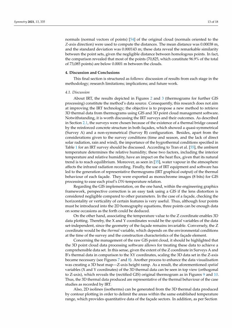
4. Discussion and Conclusions

This final section is structured as follows: discussion of results from each stage in themethodology; research limitations; implications; and future work.

4.1. Discussion

About IRT, the results depicted in Figures 2 and 3 (thermograms for further GISprocessing) constitute the method’s data source. Consequently, this research does not aimat improving the IRT technology; the objective is to propose a new method to retrieve3D thermal data from thermograms using GIS and 3D point cloud management software.Notwithstanding, it is worth discussing the IRT surveys and their outcomes. As describedin Section 2.1, the surveys were chosen because of the existence of a thermal bridge causedby the reinforced concrete structure in both façades, which showed a quasi-symmetrical(Survey A) and a non-symmetrical (Survey B) configuration. Besides, apart from theconsiderations given to the survey conditions (time and season, and the lack of directsolar radiation, rain and wind), the importance of the hygrothermal conditions specified inTable 1 for an IRT survey should be discussed. According to Tran et al. [55], the ambienttemperature determines the relative humidity; these two factors, including the interiortemperature and relative humidity, have an impact on the heat flux, given that its naturaltrend is to reach equilibrium. Moreover, as seen in [35], water vapour in the atmosphereaffects the infrared radiation recording. Finally, the use of IRT equipment and software hasled to the generation of representative thermograms (IRT graphical output) of the thermalbehaviour of each façade. They were exported as monochrome images (8 bits) for GISprocessing to ease each pixel’s DN-temperature relation.

Regarding the GIS implementation, on the one hand, within the engineering graphicsframework, perspective correction is an easy task using a GIS if the lens distortion isconsidered negligible compared to other parameters. In the case of a façade, checking thehorizontality or verticality of certain features is very useful. Thus, although four pointsmust be introduced into the 2D homography equations, three points can be enough dataon some occasions as the forth could be deduced.

On the other hand, associating the temperature value to the Z coordinate enables 3Ddata plotting. Thereby, the X and Y coordinates would be the spatial variables of the dataset-independent, since the geometry of the façade remains invariable. Conversely, the Zcoordinate would be the thermal variable, which depends on the environmental conditionsat the time of the survey and the construction characteristics of the façade element.

Concerning the management of the raw GIS point cloud, it should be highlighted thatthe 3D point cloud data processing software allows for treating these data to achieve acomprehensible data set. In this sense, given the extent of the Z coordinate in Surveys A andB’s thermal data in comparison to the XY coordinates, scaling the 3D data set in the Z-axisbecame necessary (see Figures 7 and 8). Another process to enhance the data visualisationwas creating a 3D heat map—Z-axis height ramp. As a result, the aforementioned spatialvariables (X and Y coordinates) of the 3D thermal data can be seen in top view (orthogonalto Z-axis), which reveals the (rectified GIS) original thermogram as in Figures 9 and 10.Thus, the 3D thermal data produced are representative of the thermal behaviour of the casestudies as recorded by IRT.

Also, 2D isolines (isotherms) can be generated from the 3D thermal data producedby contour plotting in order to delimit the areas within the same established temperaturerange, which provides quantitative data of the façade sectors. In addition, as per Section

Symmetry 2021, 13, 335 14 of 18

2.3, the point cloud can be discretised to create a 3D mesh with a high degree of accuracy.The combination of these isotherms and the mesh also enhance the dataset visualisation.

As to the histograms of the data from Surveys A and B, Figures 11 and 12 revealdifferent point (temperature values in Z-axis) distributions. The reason for this is multiple:the temperature range of the 3D thermal data in Survey B (1.995 ◦C) is lower than that ofSurvey A (6.710 ◦C); and there is a higher number of hot areas in the latter, which are in turnless evenly distributed. This can be seen in the lower standard deviation values of SurveyB 3D thermal data. It should be noted that the minimum and maximum temperaturevalues in the 3D thermal data produced, and their temperature ranges, differ from those ofthe original IRT data. This is because the IRT software was used to manage the original(full) thermograms, whereas the GIS rectified thermograms were smaller since only thedata within the ROI were considered in this research. Thus, the preliminary IRT extremetemperature values derive from the data out of the ROI; consequently, the 3D thermaldata’s temperature values are correct.

Regarding the ROI, it should be noted that, because of the perspective correctionin Survey B, the non-rectangular 3D thermal data set contains 73,085 points against the65,572 points of the corresponding rectangular thermogram. Considering that there are76,800 pixels in the original thermogram’s 320 × 240 pixel resolution, over 95% of thethermal information in the non-rectangular thermogram can be used for analysis, morethan that of the rectangular ROI (over 85%). The 7513 points of difference between thetwo 3D thermograms from Survey B can be seen in both Figure 6a,b, and in Figure 8b(scaled point cloud). Those points belong to the slab thermal bridge in the façade. As canbe seen in the isometric view and considering both their dimension in the Z-axis and the(gradient) colour code, the points present the greatest temperature values in Survey B’s 3Dthermal data.

The symmetry of the 3D thermal data produced via the proposed method shouldalso be discussed. As expected, Figures 7 and 8, respectively, show quasi-symmetricaland non-symmetrical values in the Z coordinate (temperature) according to their originalthermograms (Figures 2 and 3, correspondingly).

4.2. Limitations

Concerning the limitations of the proposed method, it is first worth mentioning thatIRT cannot record the temperature of hidden parts in the body (façade or object) except insome instances [13], as expected, nor those parts whose plane is in line with the direction ofthe camera. Thus, in the case of a façade as in Survey A (Figure 1), projections or overhangscannot be measured from that point of view because of being perpendicular to the façadeplane recorded via IRT. Hence, no 3D data will be obtained from those parts for that 3Dthermogram. This issue can be addressed separately for each face as in the case of twoperpendicular walls of a building with distinct temperature values among components.However, once combining the 3D thermal data of each face—in order to create a unique 3Dthermogram—there may be an overlap of data between the walls if the temperature range(Z coordinate) is high. Nonetheless, this is not a problem in cases such as Survey B, wherethe temperature range is low; thus, the 3D point set’s dispersion is low, which prevents theoperator from the data overlapping.

In relation to the image geometry, selecting a rectangular ROI is advisable in termsof graphical language. Given the angle of the IRT recording of the façade, the rectifiedthermogram contains regions with no data. This loss of thermal data could be minimised byincreasing the distance between the IRT camera and the façade so that the thermal bridgeis fully recorded. However, this entails larger pixel size in the thermograms, which meansthat the points used to conduct the rectification become less identifiable, and the thermaldata ‘resolution’ decreases. This could be considered a limitation of the IRT equipment. Inthis research, the choice of a larger (non-rectangular) ROI in Survey B allows for minimisingthe loss of thermal information from the façade because of the recording perspective, asdiscussed above.

Symmetry 2021, 13, 335 15 of 18

4.3. Implications

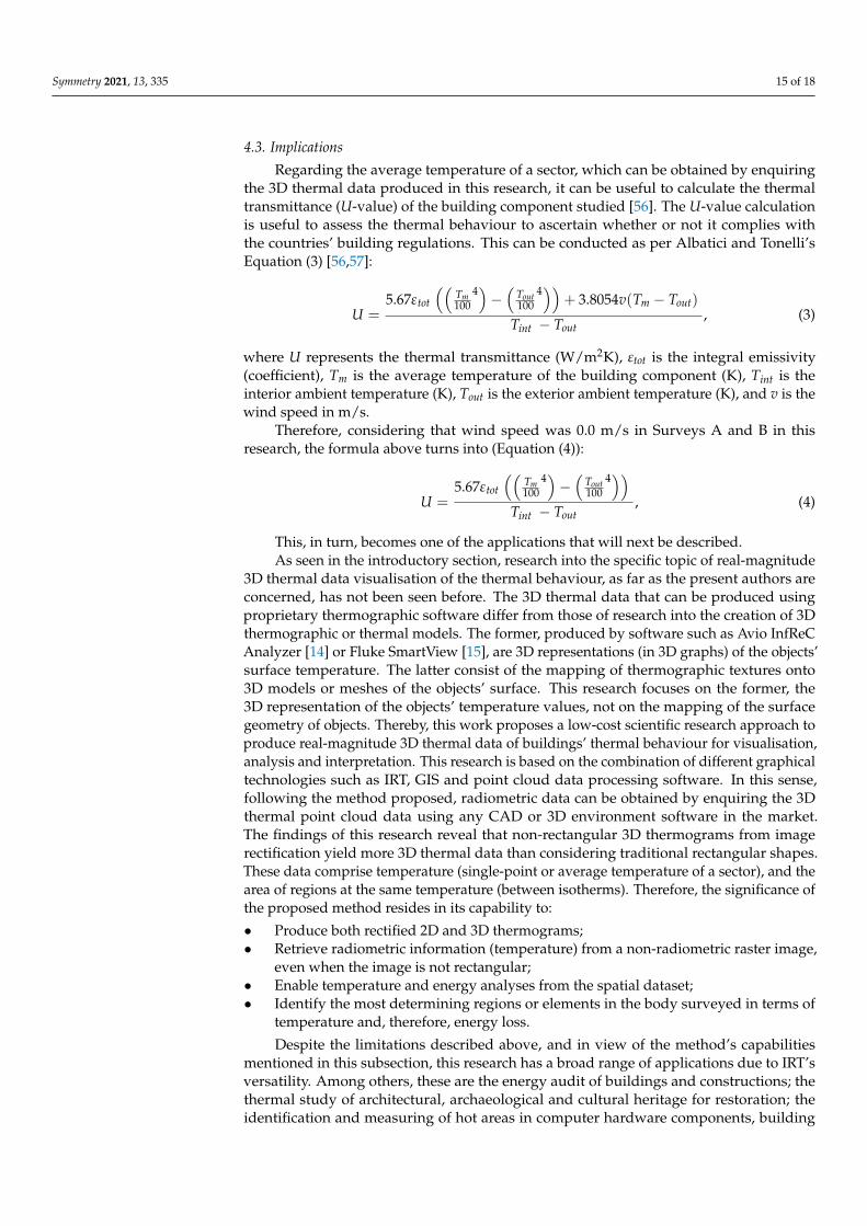
Regarding the average temperature of a sector, which can be obtained by enquiringthe 3D thermal data produced in this research, it can be useful to calculate the thermaltransmittance (U-value) of the building component studied [56]. The U-value calculationis useful to assess the thermal behaviour to ascertain whether or not it complies withthe countries’ building regulations. This can be conducted as per Albatici and Tonelli’sEquation (3) [56,57]:

U =5.67εtot

((Tm100

4)− ( Tout100

4))+ 3.8054v(Tm − Tout)

Tint − Tout, (3)

where U represents the thermal transmittance (W/m2K), εtot is the integral emissivity(coefficient), Tm is the average temperature of the building component (K), Tint is theinterior ambient temperature (K), Tout is the exterior ambient temperature (K), and v is thewind speed in m/s.

Therefore, considering that wind speed was 0.0 m/s in Surveys A and B in thisresearch, the formula above turns into (Equation (4)):

U =5.67εtot

((Tm100

4)− ( Tout100

4))Tint − Tout

, (4)

This, in turn, becomes one of the applications that will next be described.As seen in the introductory section, research into the specific topic of real-magnitude

3D thermal data visualisation of the thermal behaviour, as far as the present authors areconcerned, has not been seen before. The 3D thermal data that can be produced usingproprietary thermographic software differ from those of research into the creation of 3Dthermographic or thermal models. The former, produced by software such as Avio InfReCAnalyzer [14] or Fluke SmartView [15], are 3D representations (in 3D graphs) of the objects’surface temperature. The latter consist of the mapping of thermographic textures onto3D models or meshes of the objects’ surface. This research focuses on the former, the3D representation of the objects’ temperature values, not on the mapping of the surfacegeometry of objects. Thereby, this work proposes a low-cost scientific research approach toproduce real-magnitude 3D thermal data of buildings’ thermal behaviour for visualisation,analysis and interpretation. This research is based on the combination of different graphicaltechnologies such as IRT, GIS and point cloud data processing software. In this sense,following the method proposed, radiometric data can be obtained by enquiring the 3Dthermal point cloud data using any CAD or 3D environment software in the market.The findings of this research reveal that non-rectangular 3D thermograms from imagerectification yield more 3D thermal data than considering traditional rectangular shapes.These data comprise temperature (single-point or average temperature of a sector), and thearea of regions at the same temperature (between isotherms). Therefore, the significance ofthe proposed method resides in its capability to:

• Produce both rectified 2D and 3D thermograms;• Retrieve radiometric information (temperature) from a non-radiometric raster image,

even when the image is not rectangular;• Enable temperature and energy analyses from the spatial dataset;• Identify the most determining regions or elements in the body surveyed in terms of

temperature and, therefore, energy loss.

Despite the limitations described above, and in view of the method’s capabilitiesmentioned in this subsection, this research has a broad range of applications due to IRT’sversatility. Among others, these are the energy audit of buildings and constructions; thethermal study of architectural, archaeological and cultural heritage for restoration; theidentification and measuring of hot areas in computer hardware components, building

Symmetry 2021, 13, 335 16 of 18

services, or product quality control in the industry. Therefore, the method proposed inthis paper is initially more suitable to be applied to (approximately) flat surfaces. Thisis because a GIS is used in this research to restore the objects’ real dimensions. Thereby,the image distortion is corrected to obtain an orthogonal view that guarantees that thetemperature is represented by the Z-axis in an adequate coordinate system. In contrast,in curved and other non-flat objects, the recording of the surface temperature in the IRTsurvey is affected by the aforementioned directional emissivity [30–34]. This entails thatthe temperature (Z coordinate), initially, could not be a reliable value of the 3D thermaldata of the object. However, according to Campione et al. [58], this can be corrected inconcave and convex geometries, which increases the possible applications of the proposedmethod to non-flat objects.

4.4. Future Work

Future work on this research involves working on the bodies’ out-of-plane parts andperpendicular faces to combine their 3D thermal data with the main bodies’ data withoutoverlapping. Moreover, an ad hoc script can be developed to automate the analysis ofthe 3D thermal data produced: the creation of isotherms; the calculation of their area; thecalculation of the minimum, maximum and average temperatures; and the correspondingthermal transmittance value. Regarding the future GIS-related work, another possibleinvestigation is related to the design and placement of thermal targets on the façadesfor IRT recording. Along with the implementation of an algorithm in QGIS, this wouldautomate the image rectification, the homography between the original thermogram andthe plane of the façade. In view of the results in this research, the image rectification wouldbe performed by considering non-rectangular thermograms to increase the amount of 3Dthermal data.

Author Contributions: Conceptualization, D.A. and J.-L.A.-M.; methodology, D.A. and J.-L.A.-M.;software, D.A. and J.-L.A.-M.; validation, D.A. and J.-L.A.-M.; formal analysis, D.A. and J.-L.A.-M.;investigation, D.A. and J.-L.A.-M.; resources, D.A. and J.-L.A.-M.; data curation, D.A. and J.-L.A.-M.;writing—original draft preparation, D.A. and J.-L.A.-M.; writing—review and editing, D.A. andJ.-L.A.-M.; visualization, D.A. and J.-L.A.-M.; supervision, D.A. and J.-L.A.-M.; project administration,D.A. and J.-L.A.-M.; funding acquisition, D.A. All authors have read and agreed to the publishedversion of the manuscript.

Funding: This research was funded by Universidad de Sevilla through VI Plan Propio de Investi-gación y Transferencia (VIPPIT), grant number CONV-822 and VIPPIT-2019-II.3.

Institutional Review Board Statement: Not applicable.

Informed Consent Statement: Not applicable.

Data Availability Statement: The data presented in this study is contained within the article.

Acknowledgments: The Authors wish to acknowledge the Departamento de Expresión Gráfica eIngeniería en la Edificación of Universidad de Sevilla for access to the infrared camera and portableweather station.

Conflicts of Interest: The authors declare no conflict of interest. The funders had no role in the designof the study; in the collection, analyses, or interpretation of data; in the writing of the manuscript, orin the decision to publish the results.

References1. Sorby, S. Developing 3D spatial visualization skills. Eng. Des. Graph. J. 1999, 63, 21–32.2. Marunic, G.; Glazar, V. Spatial ability through engineering graphics education. Int. J. Technol. Des. Educ. 2013, 23, 703–715.

[CrossRef]3. Ruiz-Jaramillo, J.; Mascort-Albea, E.; Jaramillo-Morilla, A. Proposed methodology for measurement, survey and assessment of

vertical deformation of structures. Struct. Surv. 2016, 34, 276–296. [CrossRef]4. Volk, R.; Stengel, J.; Schultmann, F. Building Information Modeling (BIM) for existing buildings—Literature review and future

needs. Autom. Constr. 2014, 38, 109–127. [CrossRef]

Symmetry 2021, 13, 335 17 of 18

5. Lerma, J.L.; Navarro, S.; Cabrelles, M.; Portalés, C. Implementation of an Architectonic GIS on a Brickwork Farmhouse. InInternational Archives of the Photogrammetry, Remote Sensing and Spatial Information Sciences—ISPRS Archives; Chen, J., Jiang, J., Maas,H.-G., Eds.; International Society for Photogrammetry and Remote Sensing, Inc. (ISPRS): Beijing, China, 2008; pp. 1013–1015.

6. Previtali, M.; Erba, S.; Rosina, E.; Redaelli, V.; Scaioni, M.; Barazzetti, L. Generation of a GIS-based environment for infraredthermography analysis of buildings. In Infrared Remote Sensing and Instrumentation XX; Strojnik, M., Paez, G., Eds.; Society ofPhotographic Instrumentation Engineers: Bellingham, WA, USA, 2012; p. 85110U.

7. Yuanrong, H.; Jiaquan, D.; Shenghui, C.; Degui, P. Facade measurement of building along the roadway based on TLS and GISof project supervision. In IOP Conference Series: Earth and Environmental Science; IOP Publishing: Bristol, UK, 2018; Volume 146,p. 012027.

8. Chen, K.; Reichard, G.; Xu, X. GIS-Based Modeling of Multi-Sourced Image Data Collected for Building Facade Inspection. InConstruction Research Congress 2020; American Society of Civil Engineers: Reston, VA, USA, 2020; pp. 866–875.

9. Wang, Y.; Fan, H.; Zhou, G. Reconstructing facade semantic models using hierarchical topological graphs. Trans. GIS 2020, 24,1073–1097. [CrossRef]

10. Yue, L.; Li, H.; Zheng, X. Distorted Building Image Matching with Automatic Viewpoint Rectification and Fusion. Sensors 2019,19, 5205. [CrossRef]

11. Soycan, A.; Soycan, M. Perspective correction of building facade images for architectural applications. Eng. Sci. Technol. Int. J.2019, 22, 697–705. [CrossRef]

12. Balaras, C.A.; Argiriou, A.A. Infrared thermography for building diagnostics. Energy Build. 2002, 34, 171–183. [CrossRef]13. Glavaš, H.; Hadzima-Nyarko, M.; Hanicar Buljan, I.; Baric, T. Locating Hidden Elements in Walls of Cultural Heritage Buildings

by Using Infrared Thermography. Buildings 2019, 9, 32. [CrossRef]14. Nippon Avionics Company InfReC Analyzer NS9500 Professional; Nippon Avionics Co., Ltd.: Tokyo, Japan, 2020.15. Fluke SmartView IR Analysis Reporting Software; Fluke Corporation: Everett, WA, USA, 2013.16. Paramasivam, B. Investigation on the effects of damping over the temperature distribution on internal turning bar using Infrared

fusion thermal imager analysis via SmartView software. Meas. J. Int. Meas. Confed. 2020, 162, 107938. [CrossRef]17. Shchegolkov, A.; Shchegolkov, A.; Demidova, A. The use of nanomodified heat storage materials for thermal stabilization in

the engineering and aerospace industry as a solution for economy. In International Conference on Modern Trends in ManufacturingTechnologies and Equipment 2018 (ICMTMTE 2018); Bratan, S., Gorbatyuk, S., Leonov, S., Roshchupkin, S., Eds.; EDP Sciences:Sevastopol, Russia, 2018; Volume 224, p. 03012.

18. Alba, M.I.; Barazzetti, L.; Scaioni, M.; Rosina, E.; Previtali, M. Mapping Infrared Data on Terrestrial Laser Scanning 3D Models ofBuildings. Remote Sens. 2011, 3, 1847–1870. [CrossRef]

19. Vidas, S.; Moghadam, P.; Bosse, M. 3D thermal mapping of building interiors using an RGB-D and thermal camera. In 2013 IEEEInternational Conference on Robotics and Automation; IEEE: Piscataway, NJ, USA, 2013; pp. 2311–2318.

20. Wang, C.; Cho, Y.K.; Gai, M. As-Is 3D Thermal Modeling for Existing Building Envelopes Using a Hybrid LIDAR System. J.Comput. Civ. Eng. 2013, 27, 645–656. [CrossRef]

21. Borrmann, D.; Elseberg, J.; Nüchter, A. Thermal 3D mapping of building façades. In Advances in Intelligent Systems and Computing;Springer: Berlin/Heidelberg, Germany, 2013; Volume 193 AISC, pp. 173–182.

22. Rangel, J.; Soldan, S.; Kroll, A. 3D Thermal Imaging: Fusion of Thermography and Depth Cameras. In Proceedings of the 12thInternational Conference on Quantitative Infrared Thermography (QIRT 2014), Bordeaux, France, 7–11 July 2014.

23. Ham, Y.; Golparvar-Fard, M. 3D Visualization of thermal resistance and condensation problems using infrared thermography forbuilding energy diagnostics. Vis. Eng. 2014, 2, 1–15. [CrossRef]

24. Moghadam, P.; Vidas, S. HeatWave: The next generation of thermography devices. In Thermosense: Thermal Infrared ApplicationsXXXVI; Colbert, F.P., Hsieh, S.-J., Eds.; Society of Photographic Instrumentation Engineers: Bellingham, WA, USA, 2014; p. 91050F.

25. Moghadam, P. 3D medical thermography device. In Thermosense: Thermal Infrared Applications XXXVII; Hsieh, S.-J., Zalameda,J.N., Eds.; International Society for Optics and Photonics (SPIE): Bellingham, WA, USA, 2015; Volume 9485, p. 94851J.

26. Matsumoto, K.; Nakagawa, W.; Saito, H.; Sugimoto, M.; Shibata, T.; Yachida, S. AR Visualization of Thermal 3D Model by Hand-held Cameras. In Proceedings of the 10th International Conference on Computer Vision Theory and Applications; SCITEPRESS—Scienceand Technology Publications: Setúbal, Portugal, 2015; Volume 3, pp. 480–487.

27. Nakagawa, W.; Matsumoto, K.; de Sorbier, F.; Sugimoto, M.; Saito, H.; Senda, S.; Shibata, T.; Iketani, A. Visualization ofTemperature Change Using RGB-D Camera and Thermal Camera. In Lecture Notes in Computer Science; Including SubseriesLecture Notes in Artificial Intelligence and Lecture Notes in Bioinformatics; Springer: Berlin/Heidelberg, Germany, 2015; Volume8925, pp. 386–400, ISBN 9783319161778.

28. Natephra, W.; Motamedi, A.; Yabuki, N.; Fukuda, T.; Michikawa, T. Building Envelope Thermal Performance Analysis usingBIM-Based 4D Thermal Information Visualization. In Proceedings of the 16th International Conference on Computing in Civil andBuilding Engineering (ICCCBE2016); Yabuki, N., Makanae, K., Eds.; ICCCBE2016 Organizing Committee: Osaka, Japan, 2016;pp. 1539–1546.

29. Landmann, M.; Heist, S.; Dietrich, P.; Lutzke, P.; Gebhart, I.; Templin, J.; Kühmstedt, P.; Tünnermann, A.; Notni, G. High-speed3D thermography. Opt. Lasers Eng. 2019, 121, 448–455. [CrossRef]

30. Ianiro, A.; Cardone, G. Measurement of surface temperature and emissivity with stereo dual-wavelength IR thermography. J.Mod. Opt. 2010, 57, 1708–1715. [CrossRef]

Symmetry 2021, 13, 335 18 of 18

31. Cheng, T.Y.; Deng, D.; Herman, C. Curvature effect quantification for in-vivo IR thermography. In ASME International MechanicalEngineering Congress and Exposition, Proceedings (IMECE); NIH Public Access: Bethesda, MD, USA, 2012; Volume 2, pp. 127–133.

32. Gutierrez, E.; Castañeda, B.; Treuillet, S. Correction of Temperature Estimated from a Low-Cost Handheld Infrared Camera forClinical Monitoring. In Lecture Notes in Computer Science; Including Subseries Lecture Notes in Artificial Intelligence and LectureNotes in Bioinformatics; Springer: Berlin/Heidelberg, Germany, 2020; Volume 12002 LNCS, pp. 108–116, ISBN 9783030406042.

33. Cardone, G.; Ianiro, A.; Dello Ioio, G.; Passaro, A. Temperature maps measurements on 3D surfaces with infrared thermography.Exp. Fluids 2012, 52, 375–385. [CrossRef]

34. Greco, C.S.; Paolillo, G.; Contino, M.; Caramiello, C.; Di Foggia, M.; Cardone, G. 3D temperature mapping of a ceramic shellmould in investment casting process via infrared thermography. Quant. Infrared Thermogr. J. 2020, 17, 40–62. [CrossRef]

35. Fluke Corporation. Fluke SmartView Manual. Available online: https://dam-assets.fluke.com/s3fs-public/SmartV__pheng0100.pdf (accessed on 14 December 2020).

36. FLIR. Systems Flir Tools; FLIR: Wilsonville, OR, USA, 2018.37. ThermoWorks. Infrared Emissivity Table. Available online: https://www.thermoworks.com/emissivity-table (accessed on 12

December 2020).38. FLIR Systems. Your Perfect Palette. Available online: https://www.flir.co.uk/discover/ots/outdoor/your-perfect-palette/

(accessed on 14 December 2020).39. Al-Kindi, K.M.; Alkharusi, A.; Alshukaili, D.; Al Nasiri, N.; Al-Awadhi, T.; Charabi, Y.; El Kenawy, A.M. Spatiotemporal

Assessment of COVID-19 Spread over Oman Using GIS Techniques. Earth Syst. Environ. 2020, 4, 797–811. [CrossRef]40. Ali, S.A.; Khatun, R.; Ahmad, A.; Ahmad, S.N. Assessment of Cyclone Vulnerability, Hazard Evaluation and Mitigation Capacity

for Analyzing Cyclone Risk using GIS Technique: A Study on Sundarban Biosphere Reserve, India. Earth Syst. Environ. 2020, 4,71–92. [CrossRef]

41. Al Baky, M.A.; Islam, M.; Paul, S. Flood Hazard, Vulnerability and Risk Assessment for Different Land Use Classes Using a FlowModel. Earth Syst. Environ. 2020, 4, 225–244. [CrossRef]

42. Navarro Cerrillo, R.M.; Palacios Rodríguez, G.; Clavero Rumbao, I.; Lara, M.Á.; Bonet, F.J.; Mesas-Carrascosa, F.-J. ModelingMajor Rural Land-Use Changes Using the GIS-Based Cellular Automata Metronamica Model: The Case of Andalusia (SouthernSpain). ISPRS Int. J. Geo-Inf. 2020, 9, 458. [CrossRef]

43. Kulawiak, M.; Dawidowicz, A.; Pacholczyk, M.E. Analysis of server-side and client-side Web-GIS data processing methods onthe example of JTS and JSTS using open data from OSM and geoportal. Comput. Geosci. 2019, 129, 26–37. [CrossRef]

44. QGIS Development Team. QGIS Geographic Information System. 2020. Available online: https://qgis.org/en/site/getinvolved/faq/index.html#how-to-cite-qgis (accessed on 18 February 2021).

45. Girardeau-Montaut, D. 3D Point Cloud and Mesh Processing Software; CloudCompare: Amsterdam, The Netherlands, 2016.46. Cignoni, P.; Callieri, M.; Corsini, M.; Dellepiane, M.; Ganovelli, F.; Ranzuglia, G. MeshLab: An Open-Source Mesh Processing

Tool. In Proceedings of the Sixth Eurographics Italian Chapter Conference; Scarano, V., Chiara, R.D., Erra, U., Eds.; The EurographicsAssociation: Salerno, Italy, 2008; pp. 129–136.

47. Girardeau-Montaut, D. Colors\Height Ramp. Available online: https://www.cloudcompare.org/doc/wiki/index.php?title=Colors%5CHeight_Ramp (accessed on 21 December 2020).

48. Girardeau-Montaut, D. Rasterize. Available online: https://www.cloudcompare.org/doc/wiki/index.php?title=Rasterize(accessed on 29 December 2020).

49. Girardeau-Montaut, D. Mesh\Delaunay 2.5D (XY Plane). Available online: https://www.cloudcompare.org/doc/wiki/index.php?title=Mesh%5CDelaunay_2.5D_(XY_plane) (accessed on 29 December 2020).

50. Antón, D.; Medjdoub, B.; Shrahily, R.; Moyano, J. Accuracy evaluation of the semi-automatic 3D modeling for historical buildinginformation models. Int. J. Archit. Herit. 2018, 12, 790–805. [CrossRef]

51. Antón, D.; Pineda, P.; Medjdoub, B.; Iranzo, A. As-Built 3D Heritage City Modelling to Support Numerical Structural Analysis:Application to the Assessment of an Archaeological Remain. Remote Sens. 2019, 11, 1276. [CrossRef]

52. Lague, D.; Brodu, N.; Leroux, J. Accurate 3D comparison of complex topography with terrestrial laser scanner: Application to theRangitikei canyon (N-Z). ISPRS J. Photogramm. Remote Sens. 2013, 82, 10–26. [CrossRef]

53. Girardeau-Montaut, D. M3C2 (Plugin). Available online: https://www.cloudcompare.org/doc/wiki/index.php?title=M3C2_(plugin) (accessed on 29 December 2020).

54. Girardeau-Montaut, D. Normals\Compute. Available online: https://www.cloudcompare.org/doc/wiki/index.php?title=Normals%5CCompute (accessed on 28 November 2018).

55. Tran, Q.H.; Han, D.; Kang, C.; Haldar, A.; Huh, J. Effects of Ambient Temperature and Relative Humidity on Subsurface DefectDetection in Concrete Structures by Active Thermal Imaging. Sensors 2017, 17, 1718. [CrossRef]

56. Moyano Campos, J.J.; Antón García, D.; Rico Delgado, F.; Marín García, D. Threshold Values for Energy Loss in BuildingFaçades Using Infrared Thermography. In Sustainable Development and Renovation in Architecture, Urbanism and Engineering;Mercader-Moyano, P., Ed.; Springer: Cham, Switzerland, 2017; pp. 427–437, ISBN 978-3-319-51442-0.

57. Albatici, R.; Tonelli, A.M. Infrared thermovision technique for the assessment of thermal transmittance value of opaque buildingelements on site. Energy Build. 2010, 42, 2177–2183. [CrossRef]

58. Campione, I.; Lucchi, F.; Santopuoli, N.; Seccia, L. 3D Thermal Imaging System with Decoupled Acquisition for Industrial andCultural Heritage Applications. Appl. Sci. 2020, 10, 828. [CrossRef]