enhanced modeling of first-order plant equations of motion ... · enhanced modeling of first-order...

1 American Institute of Aeronautics and Astronautics

Enhanced Modeling of First-Order Plant Equations of Motion for Aeroelastic and Aeroservoelastic Applications

Anthony S. Pototzky1

NASA Langley Research Center, Hampton Virginia 23681

A methodology is described for generating first-order plant equations of motion for aeroelastic and aeroservoelastic applications. The description begins with the process of generating data files representing specialized mode-shapes, such as rigid-body and control surface modes, using both PATRAN and NASTRAN analysis. NASTRAN executes the 146 solution sequence using numerous Direct Matrix Abstraction Program (DMAP) calls to import the mode-shape files and to perform the aeroelastic response analysis. The aeroelastic response analysis calculates and extracts structural frequencies, generalized masses, frequency-dependent generalized aerodynamic force (GAF) coefficients, sensor deflections and load coefficients data as text-formatted data files. The data files are then re-sequenced and re-formatted using a custom written FORTRAN program. The text-formatted data files are stored and coefficients for s-plane equations are fitted to the frequency-dependent GAF coefficients using two Interactions of Structures, Aerodynamics and Controls (ISAC) programs. With tabular files from stored data created by ISAC, MATLAB generates the first-order aeroservoelastic plant equations of motion. These equations include control-surface actuator, turbulence, sensor and load modeling. Altitude varying root-locus plot and PSD plot results for a model of the F-18 aircraft are presented to demonstrate the capability.

Nomenclature A0…A6 = s-plane fit coefficients A-bar = RMS with the gust intensity factor, σ = 1 in/sec. ASE = aeroservoelastic c = generalized damping matrix D~ = generalized damping matrix including aerodynamic effects

DCM = data complex manager of the ISAC code DMAP = direct matrix abstraction program-NASTRAN programming language DMIG = direct matrix input at points-type of gridpoint data entry for NASTRAN DOF = degree of freedom DYNARES = dynamic response program (within which s-splane fits are performed) of the ISAC code EOM = equations of motion f = frequency, Hz. FE = finite element FEM = finite element model GAF = generalized aerodynamic force coefficients GLA = gust load alleviation ISAC = Interaction of Structures, Aerodynamics and Controls k = reduced frequency K = generalized stiffness matrix K~ = generalized stiffness matrix including aerodynamic effects M = generalized mass matrix Lanczos = method of NASTRAN EIGRL eigenvalue analysis LMAT = NASTRAN internally stored matrix data

https://ntrs.nasa.gov/search.jsp?R=20100031111 2020-04-18T05:28:34+00:00Z


1Aerospace Engineer, Aeroelasticity Branch, M. S. 340/ [email protected], Senior Member AIAA. M~ = generalized mass matrix including aerodynamic effects MFT = matched filter theory N0 = mean frequency of zero crossings PHIGR = NASTRAN internally stored data block for storing control mode shapes PHIGRLM = NASTRAN internally stored data block for storing load mode shapes PHRBNEW = NASTRAN internally stored data block PSD = power spectral density q = dynamic pressure RMS = root mean square s = Laplace variable σ = gust intensity factor s = Laplace variable SINV = option in EIGR eigenvalue analysis to use the enhanced inverse power method of

NASTRAN v = flight velocity vgust = gust penetration velocity

I. Introduction

Over the years NASTRAN (Ref. 1) has been a versatile tool to perform many types of aeroelastic-related analyses. It is used to perform static aeroelastic analysis, such as trim, control reversal or divergence. NASTRAN flutter analysis has been well utilized by the aircraft industry as the “work horse” for design and certification processes to clear the aircraft flight envelope. Many types of frequency response analysis can be performed, such as power spectral density (PSD), random response, RMS and mean frequency of zero crossings. With frequency analysis, users can input their own atmospheric turbulence spectra greatly expanding the versatility of NASTRAN. The more advanced capability of NASTRAN includes performing transient aeroelastic response analysis where user-supplied time-history excitations can be very general, such as those representing atmospheric turbulence. This transient capability may be coupled to simple feedback control systems to evaluate controller stability and performance with aeroelastic systems.

As many capabilities as NASTRAN has, there are many analyses with its present suite of solution capabilities that are extremely difficult or impossible to perform. Examples of analyses impossible to perform in NASTRAN are real-time simulation or nonlinear time-domain analysis of aeroelastic aircraft systems or applying “modern techniques” for designing control systems. Other examples, where NASTRAN cannot be used directly, are in matched filter theory (MFT) analysis for obtaining time-correlated gust load results; for Lyapunov equation analysis for computing RMS and No values of state variables and output quantities; or for performing aeroelastic simulation analysis where Mach number, dynamic pressure and velocity are continuously varied throughout the analysis.

Over the last few years, modern techniques of designing control systems and the fact that aircraft have become much more flexible required enhanced techniques of representing aircraft flight dynamics. Using “6 DOF” representations of aircraft to design control systems many times has insufficient fidelity to capture the necessary physics of the problem. As employed in this paper, the term “aeroservoelasticity” includes all the typical components (rigid-body translations and rotations of the


airframe, rotations of the control surfaces about their hingelines, the flexible modes of the aircraft, unsteady aerodynamics, sensor equations, and actuator dynamics), but does not include control laws.

Two software tools have been developed to generate aeroservoelastic (ASE) plant equations of motion (EOM). One is the NASA developed Interaction of Structures, Aerodynamics and Controls (ISAC) suite of modules (Ref. 2) for generating first-order aeroservoelastic plant equations of motion, which can be used in conjunction with feedback controller designs, to analyze the stability and performance of closed-loop control systems. Until the development of ISAC, all aeroelastic analyses were performed in the frequency domain. ISAC permitted aeroelastic analysis in the time domain by transforming the unsteady aerodynamics into the s-plane. Unfortunately, with the improvements of computer hardware and changes in FORTRAN compilers, over the years several of ISAC’s modules, have become victims of neglect with lack of consistent maintenance and have been rendered unusable.

Another, more recently developed software tool, which generates ASE plant EOM is available commercially from ZONA Technology (Ref. 3). ZONA’s aeroservoelastic capability employs techniques similar to those in ISAC for generating first-order ASE plant equations of motion. The software incorporating modern algorithms and numerical techniques forms state-space ASE plant equations of motion, which can be combined with control laws, and performs analyses such as gust response, control-system stability and aircraft maneuvers.

This paper describes the development of a capability to generate first-order linear-time-invariant ASE plant EOM. The capability includes: (1) NASTRAN DMAP (Ref. 4) codes; (2) a custom-written FORTRAN code; (3) modules from ISAC; and (4) MATLAB (Ref. 5) scripts. The capability was initially developed as a way to extend and supplement the capabilities resident in NASTRAN’s aeroelastic response analysis. However, it is possible to attain some of the components, such as unsteady aerodynamics, from other sources, such as the ZONA aerodynamics codes.

The functions of the four elements are:

1. NASTRAN DMAP codes - Modify NASSTRAN solution sequence 146, dynamic aeroelastic analysis, so that necessary matrices are output from NASTRAN.

2. FORTRAN code - Re-format, re-sequence and re-select the NASTRAN output matrices.

3. ISAC modules - Create s-plane fits of the unsteady aerodynamics.

4. MATLAB scripts - Assemble the final ASE plant EOM.

This paper also outlines two additional capabilities not directly related to generating first-order ASE plant EOM. The first of these is the generation of shear forces, bending moments and torsion moments using the concept of the “load mode shapes.” The second addresses a method of scaling that easily converts the aeroelastic equations of motion of a full-sized aircraft into ones of a wind-tunnel model, as described in reference 6.


A full-sized, half-model of an F-18 is used to demonstrate the first-order ASE plant EOM capabilities. With the first-order ASE plant EOM, flutter analysis in the form of root-locus results is presented with matched-point altitude variation. Additional analysis results presented in this paper are PSD and RMS of loads and accelerations from atmospheric turbulence models using first-order ASE plant EOM.

II. Aeroservoelastic System Representation

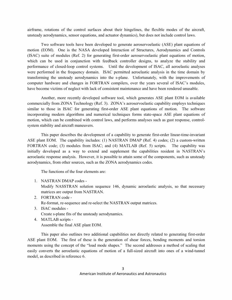
In modeling aeroservoelastic systems, there are three major components, which involve generally the aerodynamics, the aircraft structure and the control system. However, in a more detailed study, which this paper covers, it can include many more subsystem components as summarized in figure 1. The part the diagram enclosed by the dashed line can be identified as the ASE “plant” and is the part that is being addressed by the methodology described in the paper.

Some of the subsystem components like the flight control may be associated more directly with rigid-body dynamics of the aircraft and others like the load control (such as a gust load alleviation-or, GLA-system) more directly to the aircraft flexibility, but for highly flexible aircraft, all the subsystems of the aircraft affect to some degree all the other subsystem parts such as rigid-body and flexible parts. However, with extremely flexible aircraft such as the Helios, the rigid-body and elastic parts are highly coupled to the extent that one or the other cannot be modeled by itself

Figure 2. Flow Diagram of the Methodology.

FlexibleAircraft

Dynamics

Flight Control

Mode Control

Load Control

Actuators

C.S. Pos.C.S. RateC.S. Accel.

Com-mand

Attitudes

Strains

Acceler-ations

ASE Plant EOM

σ

GaussianNoise Von Karman

or DrydenGust Filter

gw&gw

Figure 1. Aeroservoelastic system diagram.


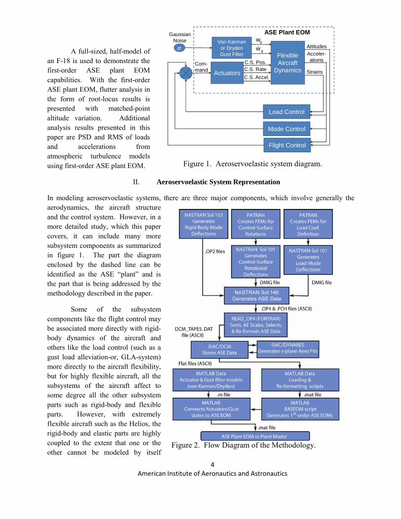
Table 1. DMAP to normalize rigid-body deflections and set frequencies to zero.

without the considerable loss of modeling fidelity. The paper will examine the methods to construct many of the subsystem components comprising the aeroservoelastic plant of the aeroservoelastic system.

III. Methodology

A description is provided of the methodology developed to generate aeroservoelastic first-order equations. The flow diagram in figure 2 shows tasks, data paths and computational software used to create, gather and store the intermediate data to produce the desired results.

It can be observed from the flow diagram that, in this methodology, several diverse software capabilities are combined to accomplish the ASE plant EOM generation task. If the data structure is known, the simplest way to connect these capabilities is by transferring the appropriate data in an ASCII format. This approach was used to avoid, or at least to minimize, data format incompatibility problems between various computational platforms. A lesser reason to use ASCII was to aid the initial development of the methodology by being able to observe data structures, types and formats directly and very easily with a simple text editor. There are exceptions to this ASCII-only philosophy, for example, when .OP2 and .mat binary files are reused by the same software capability that originally generated them.

In the following sections of the paper, salient details of the various tasks are given in order to describe the methodology including details of codes used in performing the task as well as intermediate results obtained.


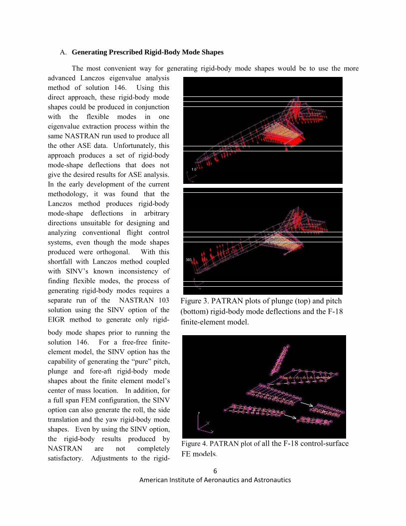
Figure 3. PATRAN plots of plunge (top) and pitch (bottom) rigid-body mode deflections and the F-18 finite-element model.

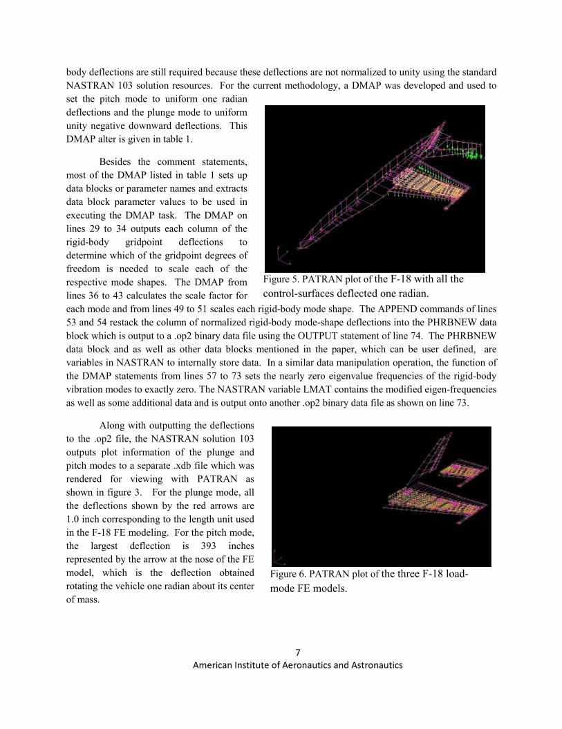
Figure 4. PATRAN plot of all the F-18 control-surface FE models.

A. Generating Prescribed Rigid-Body Mode Shapes

The most convenient way for generating rigid-body mode shapes would be to use the more advanced Lanczos eigenvalue analysis method of solution 146. Using this direct approach, these rigid-body mode shapes could be produced in conjunction with the flexible modes in one eigenvalue extraction process within the same NASTRAN run used to produce all the other ASE data. Unfortunately, this approach produces a set of rigid-body mode-shape deflections that does not give the desired results for ASE analysis. In the early development of the current methodology, it was found that the Lanczos method produces rigid-body mode-shape deflections in arbitrary directions unsuitable for designing and analyzing conventional flight control systems, even though the mode shapes produced were orthogonal. With this shortfall with Lanczos method coupled with SINV’s known inconsistency of finding flexible modes, the process of generating rigid-body modes requires a separate run of the NASTRAN 103 solution using the SINV option of the EIGR method to generate only rigid-

body mode shapes prior to running the solution 146. For a free-free finite-element model, the SINV option has the capability of generating the “pure” pitch, plunge and fore-aft rigid-body mode shapes about the finite element model’s center of mass location. In addition, for a full span FEM configuration, the SINV option can also generate the roll, the side translation and the yaw rigid-body mode shapes. Even by using the SINV option, the rigid-body results produced by NASTRAN are not completely satisfactory. Adjustments to the rigid-


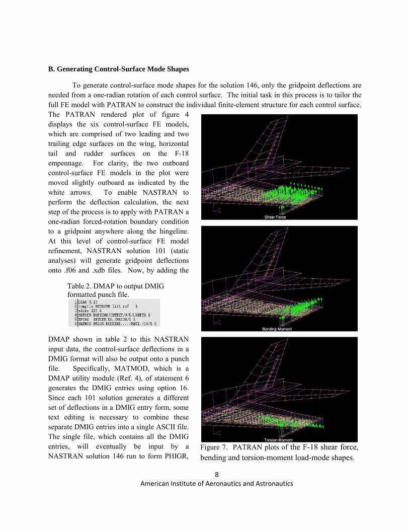
Figure 5. PATRAN plot of the F-18 with all the control-surfaces deflected one radian.

Figure 6. PATRAN plot of the three F-18 load-mode FE models.

body deflections are still required because these deflections are not normalized to unity using the standard NASTRAN 103 solution resources. For the current methodology, a DMAP was developed and used to set the pitch mode to uniform one radian deflections and the plunge mode to uniform unity negative downward deflections. This DMAP alter is given in table 1.

Besides the comment statements, most of the DMAP listed in table 1 sets up data blocks or parameter names and extracts data block parameter values to be used in executing the DMAP task. The DMAP on lines 29 to 34 outputs each column of the rigid-body gridpoint deflections to determine which of the gridpoint degrees of freedom is needed to scale each of the respective mode shapes. The DMAP from lines 36 to 43 calculates the scale factor for each mode and from lines 49 to 51 scales each rigid-body mode shape. The APPEND commands of lines 53 and 54 restack the column of normalized rigid-body mode-shape deflections into the PHRBNEW data block which is output to a .op2 binary data file using the OUTPUT statement of line 74. The PHRBNEW data block and as well as other data blocks mentioned in the paper, which can be user defined, are variables in NASTRAN to internally store data. In a similar data manipulation operation, the function of the DMAP statements from lines 57 to 73 sets the nearly zero eigenvalue frequencies of the rigid-body vibration modes to exactly zero. The NASTRAN variable LMAT contains the modified eigen-frequencies as well as some additional data and is output onto another .op2 binary data file as shown on line 73.

Along with outputting the deflections to the .op2 file, the NASTRAN solution 103 outputs plot information of the plunge and pitch modes to a separate .xdb file which was rendered for viewing with PATRAN as shown in figure 3. For the plunge mode, all the deflections shown by the red arrows are 1.0 inch corresponding to the length unit used in the F-18 FE modeling. For the pitch mode, the largest deflection is 393 inches represented by the arrow at the nose of the FE model, which is the deflection obtained rotating the vehicle one radian about its center of mass.


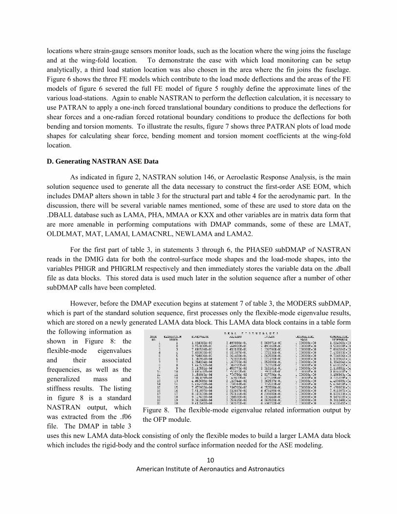
Figure 7. PATRAN plots of the F-18 shear force, bending and torsion-moment load-mode shapes.

Table 2. DMAP to output DMIG formatted punch file.

B. Generating Control-Surface Mode Shapes

To generate control-surface mode shapes for the solution 146, only the gridpoint deflections are needed from a one-radian rotation of each control surface. The initial task in this process is to tailor the full FE model with PATRAN to construct the individual finite-element structure for each control surface. The PATRAN rendered plot of figure 4 displays the six control-surface FE models, which are comprised of two leading and two trailing edge surfaces on the wing, horizontal tail and rudder surfaces on the F-18 empennage. For clarity, the two outboard control-surface FE models in the plot were moved slightly outboard as indicated by the white arrows. To enable NASTRAN to perform the deflection calculation, the next step of the process is to apply with PATRAN a one-radian forced-rotation boundary condition to a gridpoint anywhere along the hingeline. At this level of control-surface FE model refinement, NASTRAN solution 101 (static analyses) will generate gridpoint deflections onto .f06 and .xdb files. Now, by adding the

DMAP shown in table 2 to this NASTRAN input data, the control-surface deflections in a DMIG format will also be output onto a punch file. Specifically, MATMOD, which is a DMAP utility module (Ref. 4), of statement 6 generates the DMIG entries using option 16. Since each 101 solution generates a different set of deflections in a DMIG entry form, some text editing is necessary to combine these separate DMIG entries into a single ASCII file. The single file, which contains all the DMIG entries, will eventually be input by a NASTRAN solution 146 run to form PHIGR,


Table 3. The DMAP to import /combine various mode shapes and output ASE data.

which is the internal variable name for the direct input matrix. This part of the computations will be explained later in more detial, but suffice to to say now, in the PHIGR matrix, the control surface deflections are stored in separate columns, each representing one of the control-surface modes.

One of the main attractions of using the DMIG form of data entry is that only the subset of gridpoint deflections as defined by the smaller control-surface FE models need to be input into the full F-18 FE model during the execution of NASTRAN solution 146 and all the remaining gridpoint deflections of the full model are automatically set to zero values. In figure 5, the arrows represent gridpoint deflections of all the control surfaces when each is rotated one radian in the positive direction or the direction of arrows pointing downward.

C. Generating Load Mode Shapes

The process for generating the load modes was inspired by the process used to generate control-surface modes to the extent that the same steps apply in generating the deflections for either set of DMIG entries. Load mode shapes are not really mode shapes as produced by an eigenvalue analysis, but they are used the same way as mode shapes. Their function is to produce one unit gridpoint defections for shear forces and produce one radian gridpoint deflections representing their respective moment arms for the bending and torsion moments computations. Instead of defining FE structures outboard of a control-surface hingeline, the FE models used to generate load modes are defined outboard of a “load station.” These load stations can be placed across any part of the structure where loads are calculated or, using NASTRAN terminology, where loads need to be “monitored.” For the F-18 case, the load stations were placed at


Figure 8. The flexible-mode eigenvalue related information output by the OFP module.

locations where strain-gauge sensors monitor loads, such as the location where the wing joins the fuselage and at the wing-fold location. To demonstrate the ease with which load monitoring can be setup analytically, a third load station location was also chosen in the area where the fin joins the fuselage. Figure 6 shows the three FE models which contribute to the load mode deflections and the areas of the FE models of figure 6 severed the full FE model of figure 5 roughly define the approximate lines of the various load-stations. Again to enable NASTRAN to perform the deflection calculation, it is necessary to use PATRAN to apply a one-inch forced translational boundary conditions to produce the deflections for shear forces and a one-radian forced rotational boundary conditions to produce the deflections for both bending and torsion moments. To illustrate the results, figure 7 shows three PATRAN plots of load mode shapes for calculating shear force, bending moment and torsion moment coefficients at the wing-fold location.

D. Generating NASTRAN ASE Data

As indicated in figure 2, NASTRAN solution 146, or Aeroelastic Response Analysis, is the main solution sequence used to generate all the data necessary to construct the first-order ASE EOM, which includes DMAP alters shown in table 3 for the structural part and table 4 for the aerodynamic part. In the discussion, there will be several variable names mentioned, some of these are used to store data on the .DBALL database such as LAMA, PHA, MMAA or KXX and other variables are in matrix data form that are more amenable in performing computations with DMAP commands, some of these are LMAT, OLDLMAT, MAT, LAMAI, LAMACNRL, NEWLAMA and LAMA2.

For the first part of table 3, in statements 3 through 6, the PHASE0 subDMAP of NASTRAN reads in the DMIG data for both the control-surface mode shapes and the load-mode shapes, into the variables PHIGR and PHIGRLM respectively and then immediately stores the variable data on the .dball file as data blocks. This stored data is used much later in the solution sequence after a number of other subDMAP calls have been completed.

However, before the DMAP execution begins at statement 7 of table 3, the MODERS subDMAP, which is part of the standard solution sequence, first processes only the flexible-mode eigenvalue results, which are stored on a newly generated LAMA data block. This LAMA data block contains in a table form the following information as shown in Figure 8: the flexible-mode eigenvalues and their associated frequencies, as well as the generalized mass and stiffness results. The listing in figure 8 is a standard NASTRAN output, which was extracted from the .f06 file. The DMAP in table 3 uses this new LAMA data-block consisting of only the flexible modes to build a larger LAMA data block which includes the rigid-body and the control surface information needed for the ASE modeling.


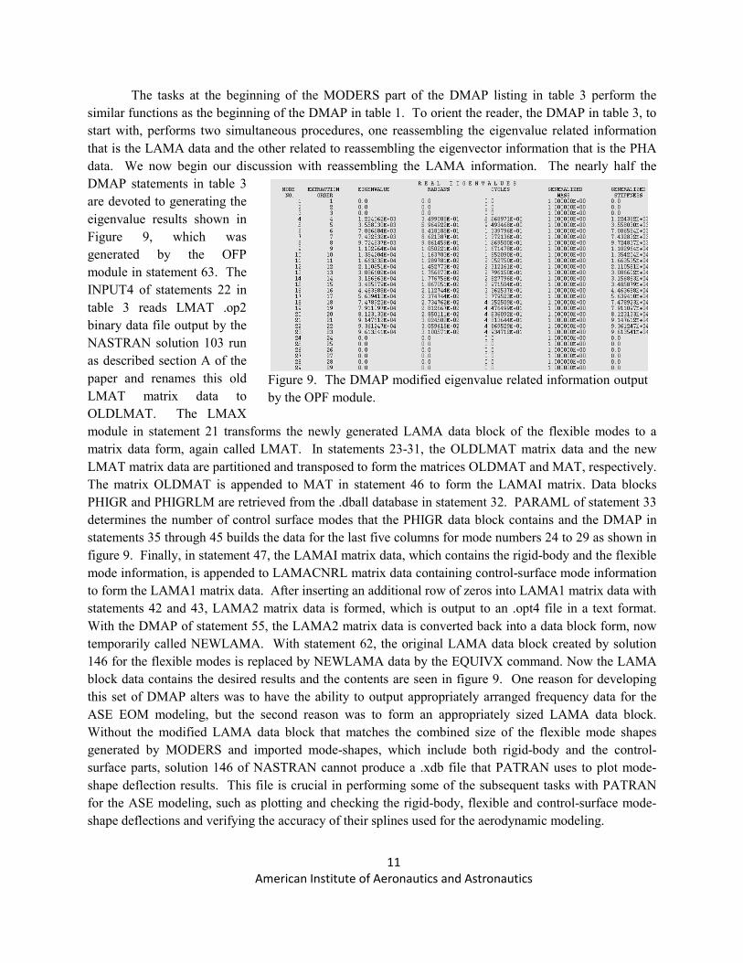
Figure 9. The DMAP modified eigenvalue related information output by the OPF module.

The tasks at the beginning of the MODERS part of the DMAP listing in table 3 perform the similar functions as the beginning of the DMAP in table 1. To orient the reader, the DMAP in table 3, to start with, performs two simultaneous procedures, one reassembling the eigenvalue related information that is the LAMA data and the other related to reassembling the eigenvector information that is the PHA data. We now begin our discussion with reassembling the LAMA information. The nearly half the DMAP statements in table 3 are devoted to generating the eigenvalue results shown in Figure 9, which was generated by the OFP module in statement 63. The INPUT4 of statements 22 in table 3 reads LMAT .op2 binary data file output by the NASTRAN solution 103 run as described section A of the paper and renames this old LMAT matrix data to OLDLMAT. The LMAX module in statement 21 transforms the newly generated LAMA data block of the flexible modes to a matrix data form, again called LMAT. In statements 23-31, the OLDLMAT matrix data and the new LMAT matrix data are partitioned and transposed to form the matrices OLDMAT and MAT, respectively. The matrix OLDMAT is appended to MAT in statement 46 to form the LAMAI matrix. Data blocks PHIGR and PHIGRLM are retrieved from the .dball database in statement 32. PARAML of statement 33 determines the number of control surface modes that the PHIGR data block contains and the DMAP in statements 35 through 45 builds the data for the last five columns for mode numbers 24 to 29 as shown in figure 9. Finally, in statement 47, the LAMAI matrix data, which contains the rigid-body and the flexible mode information, is appended to LAMACNRL matrix data containing control-surface mode information to form the LAMA1 matrix data. After inserting an additional row of zeros into LAMA1 matrix data with statements 42 and 43, LAMA2 matrix data is formed, which is output to an .opt4 file in a text format. With the DMAP of statement 55, the LAMA2 matrix data is converted back into a data block form, now temporarily called NEWLAMA. With statement 62, the original LAMA data block created by solution 146 for the flexible modes is replaced by NEWLAMA data by the EQUIVX command. Now the LAMA block data contains the desired results and the contents are seen in figure 9. One reason for developing this set of DMAP alters was to have the ability to output appropriately arranged frequency data for the ASE EOM modeling, but the second reason was to form an appropriately sized LAMA data block. Without the modified LAMA data block that matches the combined size of the flexible mode shapes generated by MODERS and imported mode-shapes, which include both rigid-body and the control-surface parts, solution 146 of NASTRAN cannot produce a .xdb file that PATRAN uses to plot mode-shape deflection results. This file is crucial in performing some of the subsequent tasks with PATRAN for the ASE modeling, such as plotting and checking the rigid-body, flexible and control-surface mode-shape deflections and verifying the accuracy of their splines used for the aerodynamic modeling.


[ ] =MCOUP

Figure 10. The generalized mass matrix.

Fortunately, the remaining part of the DMAP of table 3 used to assemble the mode-shape deflections is much more straight-forward than reassembling the eigenvalue related information. Nevertheless, it parallels the procedure for importing and assembling the modified LAMA data block. The commands in statements 20 and 32 import the rigid-body and the control-surface deflections as the PHRBNEW and PHIGR matrices, respectively. For the rigid-body and flexible mode vectors, the APPEND of statement 56 stacks them and calls the result, PHIA1. In statements 67 to 80, the DMAP processing determines the sizes of the imported control-surface vectors, and then converts them to A-set size, if necessary. The final A-set sized result is called the UA matrix. The previously formed PHIA1 matrix is appended to UA to form PHIA2. With the PHIA2 matrix containing the rigid-body, flexible and the control-surface mode shapes and with the MMAA matrix, which is the FEM mass matrix, the SMPYAD processor of statement 98 performs the matrix operation expressed in equation (1)

A2][MMAA][PHI [PHIA2]=[MCOUP] T (1)

This operation computes the generalized mass matrix. The MCOUP matrix is now suitable for ASE EOM modeling and is placed on the .op4 file with the OUTPUT4 command of statement 100.

Figure 10 shows the four corners of the generalized mass matrix, [MCOUP]. The upper left corner of this matrix contains rigid-body mass and pitch-inertia terms and the first three unity-mass terms of the flexible modes. The last six columns of the upper right corner contain the control surface mass-coupling terms. The last six columns of the bottom right corner contain six diagonal elements representing the rotational inertia terms of the control surfaces. The bottom left corner mass-coupling terms are the transposes of the terms of upper right corner. Finally, the EQUIVX command of statement 97 replaces the PHA data block, which contains only the flexible mode shapes originally generated by MODERS subDMAP, with the new PHIA2 mode shapes. The modified PHA will be used later in performing the spline and aerodynamic calculations.

Similar to statement 98, the statement 105 of table 3 performs a triple matrix multiplication to generate the mode-displacement coefficients, as expressed in equation (2)

2][KXX][PHIA [UALM]=[LDCOEF] T (2)

where UALM contains the load mode vectors (also refer to as direction vectors), KXX contains the FE model stiffness matrix, and PHIA2 contains the rigid-body, flexible and the control-surface mode shapes. Despite the simplicity of this triple matrix multiplication task, it is instructive to understand each step


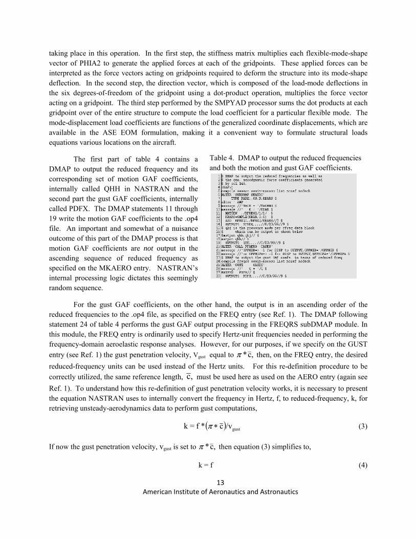
Table 4. DMAP to output the reduced frequencies and both the motion and gust GAF coefficients.

taking place in this operation. In the first step, the stiffness matrix multiplies each flexible-mode-shape vector of PHIA2 to generate the applied forces at each of the gridpoints. These applied forces can be interpreted as the force vectors acting on gridpoints required to deform the structure into its mode-shape deflection. In the second step, the direction vector, which is composed of the load-mode deflections in the six degrees-of-freedom of the gridpoint using a dot-product operation, multiplies the force vector acting on a gridpoint. The third step performed by the SMPYAD processor sums the dot products at each gridpoint over of the entire structure to compute the load coefficient for a particular flexible mode. The mode-displacement load coefficients are functions of the generalized coordinate displacements, which are available in the ASE EOM formulation, making it a convenient way to formulate structural loads equations various locations on the aircraft.

The first part of table 4 contains a DMAP to output the reduced frequency and its corresponding set of motion GAF coefficients, internally called QHH in NASTRAN and the second part the gust GAF coefficients, internally called PDFX. The DMAP statements 11 through 19 write the motion GAF coefficients to the .op4 file. An important and somewhat of a nuisance outcome of this part of the DMAP process is that motion GAF coefficients are not output in the ascending sequence of reduced frequency as specified on the MKAERO entry. NASTRAN’s internal processing logic dictates this seemingly random sequence.

For the gust GAF coefficients, on the other hand, the output is in an ascending order of the reduced frequencies to the .op4 file, as specified on the FREQ entry (see Ref. 1). The DMAP following statement 24 of table 4 performs the gust GAF output processing in the FREQRS subDMAP module. In this module, the FREQ entry is ordinarily used to specify Hertz-unit frequencies needed in performing the frequency-domain aeroelastic response analyses. However, for our purposes, if we specify on the GUST entry (see Ref. 1) the gust penetration velocity, Vgust equal to ,c * π then, on the FREQ entry, the desired reduced-frequency units can be used instead of the Hertz units. For this re-definition procedure to be correctly utilized, the same reference length, ,c must be used here as used on the AERO entry (again see Ref. 1). To understand how this re-definition of gust penetration velocity works, it is necessary to present the equation NASTRAN uses to internally convert the frequency in Hertz, f, to reduced-frequency, k, for retrieving unsteady-aerodynamics data to perform gust computations,

( ) /vc *f=k gust∗π (3)

If now the gust penetration velocity, vgust is set to ,c * π then equation (3) simplifies to,

k = f (4)


With this gust penetration velocity substitution, the frequencies specified in the FREQ entry are now used as reduced frequencies by NASTRAN.

E. READ_OP4 Fortran Program

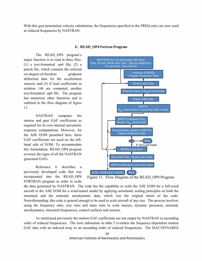
The READ_OP4 program’s major function is to read in three files: (1) a text-formatted .op4 file; (2) a punch file, which contains the selected six-degree-of-freedom gridpoint deflection data for the acceleration sensors; and (3) if load coefficients in solution 146 are computed, another text-formatted .op4 file. The program has numerous other functions and is outlined in the flow diagram of figure 11.

NASTRAN computes the motion and gust GAF coefficients as required for its own internal aeroelastic response computations. However, for the ASE EOM presented here, these GAF coefficients are used on the left-hand side of EOM. To accommodate this formulation, READ_OP4 program reverses the signs of all the NASTRAN generated GAFs.

Reference 6 describes a previously developed code that was incorporated into the READ_OP4 FORTRAN program in order to scale the data generated by NASTRAN. The code has the capability to scale the ASE EOM for a full-sized aircraft to the ASE EOM for a wind-tunnel model by applying aeroelastic scaling principles on both the structural and the unsteady aerodynamic data, which was the original intent of the code. Notwithstanding, this code is general enough to be used to scale aircraft of any size. The process involves using the frequency ratio, size ratio and mass ratio to scale masses, dynamic pressures, unsteady aerodynamics, structural frequencies, control surfaces and sensors.

As mentioned previously the motion GAF coefficients are not output by NASTRAN in ascending order of reduced frequencies. The isort subroutine in table 5 re-orders the frequency-dependent motion GAF data with an indexed array to an ascending order of reduced frequencies. The ISAC/DYNARES

Figure 11. Flow Diagram of the READ_OP4 Program.


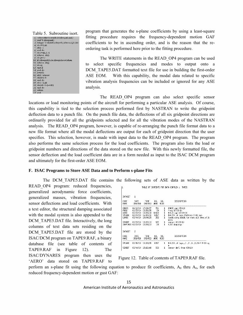
Table 5. Subroutine isort.

Figure 12. Table of contents of TAPE9.RAF file.

program that generates the s-plane coefficients by using a least-square fitting procedure requires the frequency-dependent motion GAF coefficients to be in ascending order, and is the reason that the re-ordering task is performed here prior to the fitting procedure.

The WRITE statements in the READ_OP4 program can be used to select specific frequencies and modes to output onto a DCM_TAPE5.DAT formatted text file for use in building the first-order ASE EOM. With this capability, the modal data related to specific vibration analysis frequencies can be included or ignored for any ASE analysis.

The READ_OP4 program can also select specific sensor locations or load monitoring points of the aircraft for performing a particular ASE analysis. Of course, this capability is tied to the selection process performed first by NASTRAN to write the gridpoint deflection data to a punch file. On the punch file data, the deflections of all six gridpoint directions are ordinarily provided for all the gridpoints selected and for all the vibration modes of the NASTRAN analysis. The READ_OP4 program, however, is capable of re-arranging the punch file format data to a new file format where all the modal deflections are output for each of gridpoint direction that the user specifies. This selection, however, is made with input data to the READ_OP4 program. The program also performs the same selection process for the load coefficients. The program also lists the load or gridpoint numbers and directions of the data stored on the new file. With this newly formatted file, the sensor deflection and the load coefficient data are in a form needed as input to the ISAC DCM program and ultimately for the first-order ASE EOM.

F. ISAC Programs to Store ASE Data and to Perform s-plane Fits

The DCM_TAPE5.DAT file contains the following sets of ASE data as written by the READ_OP4 program: reduced frequencies, generalized aerodynamic force coefficients, generalized masses, vibration frequencies, sensor deflections and load coefficients. With a text editor, the structural damping associated with the modal system is also appended to the DCM_TAPE5.DAT file. Interactively, the long columns of text data sets residing on the DCM_TAPE5.DAT file are stored by the ISAC/DCM program on TAPE9.RAF, a binary database file (see table of contents of TAPE9.RAF in Figure 12). The ISAC/DYNARES program then uses the ‘AERO’ data stored on TAPE9.RAF to perform an s-plane fit using the following equation to produce fit coefficients, A0 thru A6, for each reduced frequency-dependent motion or gust GAF:


∑=

=+

4i

1iikj,2,i

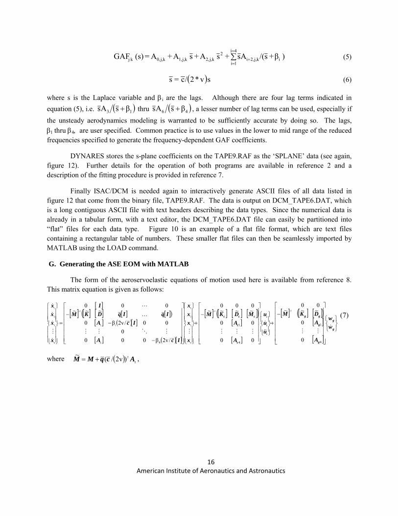
2kj,2,kj,1,kj,0,kj ) β+ s/(As+ s A+s A+A=(s) GAF (5)

( ) sv*2/c= s (6)

where s is the Laplace variable and βi are the lags. Although there are four lag terms indicated in equation (5), i.e. ( )13 βsAs + thru ( )46 βsAs + , a lesser number of lag terms can be used, especially if the unsteady aerodynamics modeling is warranted to be sufficiently accurate by doing so. The lags, β1 thru β4, are user specified. Common practice is to use values in the lower to mid range of the reduced frequencies specified to generate the frequency-dependent GAF coefficients.

DYNARES stores the s-plane coefficients on the TAPE9.RAF as the ‘SPLANE’ data (see again, figure 12). Further details for the operation of both programs are available in reference 2 and a description of the fitting procedure is provided in reference 7.

Finally ISAC/DCM is needed again to interactively generate ASCII files of all data listed in figure 12 that come from the binary file, TAPE9.RAF. The data is output on DCM_TAPE6.DAT, which is a long contiguous ASCII file with text headers describing the data types. Since the numerical data is already in a tabular form, with a text editor, the DCM_TAPE6.DAT file can easily be partitioned into “flat” files for each data type. Figure 10 is an example of a flat file format, which are text files containing a rectangular table of numbers. These smaller flat files can then be seamlessly imported by MATLAB using the LOAD command.

G. Generating the ASE EOM with MATLAB

The form of the aeroservoelastic equations of motion used here is available from reference 8. This matrix equation is given as follows:

[ ][ ]

[ ]( [ ] [ ] [ ])[ ] ( )[ ]

[ ] ( )[ ]

[ ] [ ]( [ ] [ ])[ ]

[ ]

[ ] [ ]( [ ])[ ]

[ ]⎭⎬⎫

⎩⎨⎧

⎥⎥⎥⎥⎥⎥

⎦

⎤

⎢⎢⎢⎢⎢⎢

⎣

⎡−

+⎪⎭

⎪⎬

⎫

⎪⎩

⎪⎨

⎧

⎥⎥⎥⎥⎥⎥

⎦

⎤

⎢⎢⎢⎢⎢⎢

⎣

⎡−

+

⎪⎪⎪

⎭

⎪⎪⎪

⎬

⎫

⎪⎪⎪

⎩

⎪⎪⎪

⎨

⎧

⎥⎥⎥⎥⎥⎥

⎦

⎤

⎢⎢⎢⎢⎢⎢

⎣

⎡

−

−−

=

⎪⎪⎪

⎭

⎪⎪⎪

⎬

⎫

⎪⎪⎪

⎩

⎪⎪⎪

⎨

⎧−−−

g

g

g

g

gg

c

c

ccc

ww

A

ADKM

uuu

A

AMDKM

x

xxx

IcA

IcAIqIqDK

IM

x

xxx

c

c

c

&MM&&

&

MMMMMOMM

K

L

&

M

&

&

&

4

1

4

1

4 0

0

~~~00

00

00

~~~000

~

/2vβ0000

00/2vβ0

~~000

~ 11

6

3

2

1

6

13

1

6

3

2

1

(7)

where ( ) 2

2)2v/(~ AcqMM += ,


Table 6. MATLAB script, baseom.m.

0

~ AqKK += ,

( )( ) 12v/~ AcqDD +=

and 22

1 vρ=q . The[ ]0A thru [ ]6A matrices contain the coefficients obtained by fitting equation (5), and their row/column dimensions are the same as those of the motion and the gust GAF coefficient matrices. Generally four normalized aerodynamic lags are used and are depicted as, β1 thru β4, in equation (7). The state variables, { }1x and { }2x are the generalized displacements and velocities for all the modes, respectively. The variables{ }3x thru{ }6x are the states associated with aerodynamic lags. The{ }u ,{ }u& and{ }u&& are the displacements, rates and accelerations of the control surfaces produced by the actuator models. The gw and gw& inputs representing the vertical turbulence velocity and acceleration, respectively.

The mass coupling terms together with accelerations caused by the control-surface motion produce in ASE equation (7) inertial force effects on the airframe or, stated more graphically, produce a “dog wagging tail” effect. This force is present even when the aerodynamic forces are zero. Including this effect is an important part of ASE modeling, especially when considering that controlling this force can be used to reduce buffet loads (Ref. 9).


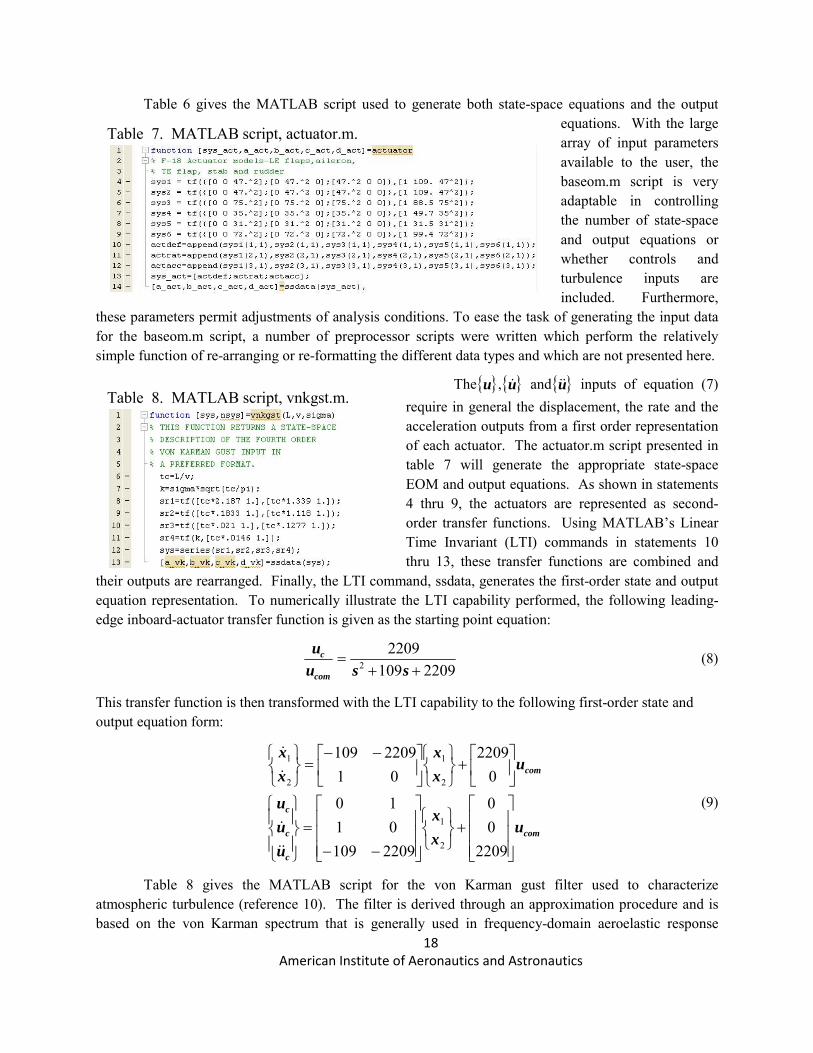
Table 7. MATLAB script, actuator.m.

Table 8. MATLAB script, vnkgst.m.

Table 6 gives the MATLAB script used to generate both state-space equations and the output equations. With the large array of input parameters available to the user, the baseom.m script is very adaptable in controlling the number of state-space and output equations or whether controls and turbulence inputs are included. Furthermore,

these parameters permit adjustments of analysis conditions. To ease the task of generating the input data for the baseom.m script, a number of preprocessor scripts were written which perform the relatively simple function of re-arranging or re-formatting the different data types and which are not presented here.

The{ }u ,{ }u& and{ }u&& inputs of equation (7) require in general the displacement, the rate and the acceleration outputs from a first order representation of each actuator. The actuator.m script presented in table 7 will generate the appropriate state-space EOM and output equations. As shown in statements 4 thru 9, the actuators are represented as second-order transfer functions. Using MATLAB’s Linear Time Invariant (LTI) commands in statements 10 thru 13, these transfer functions are combined and

their outputs are rearranged. Finally, the LTI command, ssdata, generates the first-order state and output equation representation. To numerically illustrate the LTI capability performed, the following leading-edge inboard-actuator transfer function is given as the starting point equation:

22091092209

2 ++=

ssuucom

c (8)

This transfer function is then transformed with the LTI capability to the following first-order state and output equation form:

com

c

c

c

com

uxx

uuu

uxx

xx

⎥⎥⎥

⎦

⎤

⎢⎢⎢

⎣

⎡+

⎭⎬⎫

⎩⎨⎧

⎥⎥⎥

⎦

⎤

⎢⎢⎢

⎣

⎡

−−=

⎪⎭

⎪⎬

⎫

⎪⎩

⎪⎨

⎧

⎥⎦

⎤⎢⎣

⎡+

⎭⎬⎫

⎩⎨⎧

⎥⎦

⎤⎢⎣

⎡ −−=

⎭⎬⎫

⎩⎨⎧

220900

22091090110

02209

012209109

2

1

2

1

2

1

&&

&

&

&

(9)

Table 8 gives the MATLAB script for the von Karman gust filter used to characterize atmospheric turbulence (reference 10). The filter is derived through an approximation procedure and is based on the von Karman spectrum that is generally used in frequency-domain aeroelastic response


Figure 13. Open-loop root-locus flutter analysis performed from 30,000 feet to sea level at 0.5 Mach on an F-18 FEM using the symmetrical modes.

Figure 14. PSD of wing-tip and root acceleration at 15,000 ft. altitude and 0.50 Mach.

analysis as in NASTRAN solution 146. The script generates both gw and gw& characterizing atmospheric

turbulence. The MATLAB script vnkgst.m performs with LTI the same three tasks of representing, combining the gust-filter transfer-function equation and generating the state and output equations for gw

and gw& as the actuator.m script.

IV. Results

Using the example F-18 aircraft, the ASE EOM developed with the methodology described in the paper will be employed to perform an open-loop flutter analysis and a turbulence analysis. The flight analysis conditions chosen are 0.5 Mach number at several altitudes.

The first result is a flutter root-locus with altitude variation at matched point conditions from 30,000 feet to sea level. The data were obtained from the standard-atmospheric tables of reference 11, which was tabulated into MATLAB script form. Structural damping of 2% was chosen. Figure 13 shows the flutter root-locus results of an open-loop, free-free symmetrical configuration, which includes the plunge and pitch rigid-body modes. The roots generally follow a stabilizing direction with increasing dynamic pressure, except for the 13th structural mode.

The second set of results is from a turbulence analysis at 15,000 feet. The power-spectral-density function of the wing root and tip vertical accelerations are shown in Figure 14. The gust intensity was set at a nominal value of 1 inch/sec in the application of the von Karman spectrum and the gust is applied in


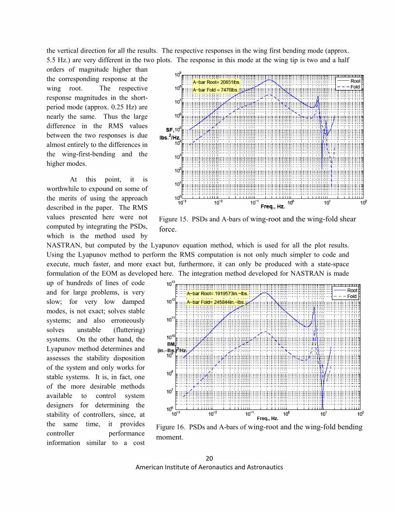
Figure 15. PSDs and A-bars of wing-root and the wing-fold shear force.

Figure 16. PSDs and A-bars of wing-root and the wing-fold bending moment.

the vertical direction for all the results. The respective responses in the wing first bending mode (approx. 5.5 Hz.) are very different in the two plots. The response in this mode at the wing tip is two and a half orders of magnitude higher than the corresponding response at the wing root. The respective response magnitudes in the short-period mode (approx. 0.25 Hz) are nearly the same. Thus the large difference in the RMS values between the two responses is due almost entirely to the differences in the wing-first-bending and the higher modes.

At this point, it is worthwhile to expound on some of the merits of using the approach described in the paper. The RMS values presented here were not computed by integrating the PSDs, which is the method used by NASTRAN, but computed by the Lyapunov equation method, which is used for all the plot results. Using the Lyapunov method to perform the RMS computation is not only much simpler to code and execute, much faster, and more exact but, furthermore, it can only be produced with a state-space formulation of the EOM as developed here. The integration method developed for NASTRAN is made up of hundreds of lines of code and for large problems, is very slow; for very low damped modes, is not exact; solves stable systems; and also erroneously solves unstable (fluttering) systems. On the other hand, the Lyapunov method determines and assesses the stability disposition of the system and only works for stable systems. It is, in fact, one of the more desirable methods available to control system designers for determining the stability of controllers, since, at the same time, it provides controller performance information similar to a cost


Figure 17. PSDs and A-bars of wing-root and the wing-fold torsion moment.

function.

The third set of results is loads at the wing-root and the wing-fold locations. Both the root and fold results are plotted for the shear-force, bending- and torsion-moment loads on figures 15, 16, and 17, respectively. For the wing-root loads, the major contributions to the RMSs come from the short period mode similar to the wing-root acceleration RMSs, which also comes from the short-period mode contributions. However, at the wing fold location, the shear-force and bending-moment ratios of the square-root of short-period values to their respective RMSs is much less than one, indicating a greater contribution from the structural modes. Strengthening this argument are the PSD plots at the wing-fold location that show the peaks of the short-period and the first bending modes are at more comparable levels. The torsion moment loads stand out as an exception. At both the wing-root and wing-fold locations, the square-root of the peak and RMS ratios for both cases is nearly one. In figure 17 of the torsion moment result, the short-period PSD peaks substantially overwhelm all the other peaks making the short-period mode the dominant player for the torsion moment load in terms of RMS.

A final note on the load calculation methodology developed and presented here in the paper. Although, the mode-displacement coefficients were computed using NASTRAN’s aeroelastic response analyses and DMAP capabilities; it is interesting to note that the author found no simple or easy way to use these load coefficients to perform aeroelastic gust load response analysis in NASTRAN. The aeroelastic response analysis does not appear to be set up or able to perform load response analysis. These coefficients were, however, incorporated into the state-space formulation developed here with almost no effort to obtain the load results presented here.

V. Conclusions

A methodology for generating enhanced first-order aeroservoelastic plant equations of motion was presented. The paper gives first, a flow diagram of the aeroservoelastic system, then a flow chart of the methodology. Intermediate results of each step of using the methodology are provided as a guide to implementing the procedures. Numerous DMAP alters were also given in tables throughout the paper which were incorporated in NASTRAN to perform the many non-standard tasks. A flow chart of the


READ_OP4 code also is provided, which reads formatted text and punch files, re-formats and re-sequences NASTRAN generated output data into a form usable in ISAC and ultimately in MATLAB. The paper outlined the data storing and s-plane fitting capabilities of the ISAC programs. The form of the first-order ASE EOM and the MATLAB script used to generate them were presented. An altitude-varying root-locus result, PSD of wing-tip and root accelerations and PSDs of loads at wing root and fold locations along with their respective RMSs were presented to demonstrate the enhanced ASE capability.


References

1. Rodden, William R. and Johnson, Erwin H.: MSC/NASTRAN Aeroelastic Analysis, USER’S GUIDE, V68, The MacNeal-Schwendler Corporation, 1994.

2. Peel, Ellwood L. and Adams, William M.: “A Digital Program For Calculating the Interaction Between Flexible Structures, Unsteady Aerodynamics and Active Controls,” NASA TM-80040, Jan. 1979.

3. No authors listed: ZAERO Version 6.0; User’s Manual, Zona Technologies, Scottsdale, AZ, May 2002.

4. Reymond, Michael: MD NASTRAN 2006 DMAP Programmer’s Guide, The MacNeal-Schwendler Corporation, 2006.

5. Using MATLAB Version 6, The MathWorks, Inc., Natick, MA, 2000. 6. Pototzky, Anthony S.:“Scaling Laws Applied to a Modal Formulation of the Aeroservoelastic

Equations,” 43rd AIAA Structure, Structural Dynamics, and Materials Conference, Denver, Colorado, April 2002.

7. Adams, Jr., William M.; Tiffany, Sherwood H.; “Newsom, Jerry R. and Peele, Ellwood L.: STABCAR- A Program for Finding Characteristic Roots of Systems Having Transcendental Stability Matrices,” NASA TP-2165, June 1984.

8. Mukhopadhyay, Vivek; Newsom, Jerry R.; and Abel, Irving: “A Method for Obtaining Reduced-Order Control Laws for High-Order Systems Using Optimization Techniques,” NASA Tech. Paper 1876, August 1981.

9. Moses, Robert W., Pototzky, Anthony S. et al: “Controlling buffeting loads by rudder and piezo-actuation,” International Forum for Aeroelasticity and Dynamics, Munich, Germany, 2005.

10. Pototzky, A. S., Zeiler, T. A and Perry III, B.: “Calculating Time-Correlated Gust Loads Using Matched-Filter and Random Process Theories,” Journal of Aircraft, Vol. 28, No. 5, 1991, p 346-352.

11. U. S. Standard Atmosphere, Washington, DC, 1962.

enhanced modeling of first-order plant equations of motion ... · enhanced modeling of first-order...

Documents