ensc 835: high-performance networks cmpt 885: …
TRANSCRIPT

1
ENSC 835: HIGH-PERFORMANCE NETWORKS
CMPT 885: SPECIAL TOPICS: HIGH-PERFORMANCE NETWORKS
GPRS: Wireless links, multiple base transmitter stations, base station controller and cell update
Fall 2003
Final Project Report
Frank Zimmermann, Renju Narayanan
www.sfu.ca/~frz/835

2
Table of Contents: 1. Abstract ......................................................................................................... 3 2. Introduction .................................................................................................... 4 3. Technical description ..................................................................................... 5
3.1 GPRS overview......................................................................................... 5 3.2 GSM specifications ................................................................................... 5 3.3 GSM and GPRS Network overview........................................................... 6 3.4 GMM states .............................................................................................. 7 3.5 Cell update.............................................................................................. 10
4. Implementation in OPNET: .......................................................................... 12 4.1 BSC node model:.................................................................................... 13 4.2 BTS node model: .................................................................................... 15 4.3 Mobile Station: ........................................................................................ 16
5. Simulations: ................................................................................................. 21 5.1 Simulation 1: ........................................................................................... 21 5.2 Simulation 2: ........................................................................................... 22 5.3 Simulation 3: ........................................................................................... 24 5.4 Simulation 4: ........................................................................................... 26
6. Future work:................................................................................................. 29 7. Discussion and Conclusions: ....................................................................... 29 8. References .................................................................................................. 30 Appendix A, Frequency usage: ........................................................................ 31 Appendix B, Code listing: ..................................................................................32

3
1. Abstract
The General Packet Radio Service (GPRS) is a new packed switched service which is an addition to the Global System for Mobile communication (GSM), a wireless cellular network. It supplements today's circuit switched data and short message service. This report describes a project that has been done as an enhancement to an existing GPRS OPNET model; OPNET is a network simulation tool. The current model consists of multiple Mobile Stations (MS), which are connected through wired links to the Base Transmitter Station (BTS). In the real GPRS Network there is a Base Station Controller (BSC) situated between the BTSs and the Serving GPRS Support Node (SGSN). In the real world there are also no wired links between the MSs and BTS. This project attempts to reduce a few of these gaps. The reader will be presented first with an introduction to GSM and GPRS. Next the report describes the existing GPRS OPNET model and gives the details of the project implementation followed by the discussion of simulation results and future work.

4
2. Introduction
The goal of this project is to enhance the existing OPNET General Packet Radio Service (GPRS) model by enhancing the implementation of Base Station Subsystem (BSS). The current model consists of multiple Mobile Stations (MS) which are connected through wired links to the Base Transmitter Station (BTS). The BTS routes the data from the MS to the Serving GPRS Support Node (SGSN), receives packets from the SGSN and routes them to the MS, according to the Temporary Logical Link Identifier (TLLI) value attached to the packets.
The Base Station Controller (BSC) which is in a real GPRS network situated between the BTSs and the Serving GPRS Support Node (SGSN) routes the traffic to different BTSs and controls the cell update (when the MS moves from one cell to another cell).
The wired links in the present model will be replaced by wireless links and a BSC will be implemented in order to support multiple BTS. Cell reselections of MSs will be simulated after that.
The goals of the project are: • Enhance the BSS implemented in the existing OPNET GPRS model by
the addition of a BSC to support multiple BTSs. • Replace the wired links in the present model by wireless links. • Simulate the cell reselection of MSs.

5
3. Technical description
3.1 GPRS overview GPRS is a standard for packed switched mobile networks introduced by the European Telecommunications Standards Institute (ETSI). It is designed as an addition to GSM which is a 2nd generation digital cellular network. Time Division Multiple Access (TDMA) and Frequency Division Multiple Access (FDMA) are implemented in GSM. It also uses circuit switching technology which is not very efficient for handling data transmissions varying bit rates like WAP, web browsing, email, navigation systems and location based services. In contrast to GSM (which supports 9.6 kbps) GPRS offers up to 171.2 kbps through multislot capability and different channel coding schemes. GPRS handles bandwidth more efficiently, several users can share the same timeslots / channels. Network operators can offer cheaper wireless internet access by billing for traffic volume instead of time. It is seen as the next step to 3rd generation cellular wireless networks like Universal Mobile Telecommunications Systems (UMTS).
3.2 GSM specifications GSM uses frequencies at 900 MHz and 1800 MHz, in North America 1900 MHz. Personal Communications Systems (PCS) 1900:
Uplink (MS – BTS) 1850.2 MHz – 1909.8 MHz
Downlink (BTS – MS) 1930.2 MHz – 1989.8 MHz
Channel bandwidth 200 kHz
Modulation Gaussian minimum shift keying (GMSK) Table 1: PCS 1900
Uplink and downlink frequencies are allocated in pairs; in PCS 1900 the distance between uplink and downlink frequencies is 80 MHz. BTS usually use more than one frequency to support many users. On each frequency TDMA frames with 8 timeslots are sent. The first frequency used by a BTS is also called “BCCH frequency” because the broadcast control channel (BCCH) is transmitted in one of the timeslots there. The BCCH is used by the mobile stations for channel measurements.

6
3.3 GSM and GPRS Network overview
Figure 1: GPRS network structure
The GGSN is the interface to the external packet network. It is connected to the SGSN via a connection that uses Internet Protocol (IP) and is also concerned with collecting all charges regarding external network resources [8]. The core element of the GPRS network is the SGSN, it is responsible for packet switching, authentication, ciphering, data compression and also charging. The SGSN is situated at the same level as the Mobile Switching Center (MSC) in GSM. The MSC is originally an ISDN exchange that has been modified for the use in a cellular network. One of the consequences of that is that the radio resource management (RR) functions were relocated at the BSC. One of the major functions of the BSC is to evaluate measurement results from MSs and BTSs and control handover and power control for GSM connections. The BTS enables wireless connections of MSs to the network over the air interface and performs all layer 1 functions like channel coding, interleaving, burst generating, GMSK modulation and demodulation. [8] Subscriber information like telephone numbers, service characteristics and service limitations are stored in the HLR. GPRS MSs support in addition to GSM MSs new protocols for RR, GPRS mobility management (GMM) and session management functions. They also have new channel coding schemes and are enabled for multislot transmissions.

7
3.4 GMM states
Three different states for Mobility Management (MM) have been defined in the standard reduce the signaling traffic when MSs are not transmitting or receiving data. The three MM states are:
• GMM IDLE • GMM STANDBY • GMM READY
These global states are managed in the MS and in the SGSN for each MS. The transitions between the states are slightly different on the MS and SGSN sides. GMM IDLE state: When a GPRS mobile is in the IDLE state, it is not attached for GPRS service. No GPRS mobility context is established between the MS and the SGSN i.e.; no information related to the MS is stored at SGSN level. GMM STANDBY state: When a GPRS mobile is in the STANDBY state, it is attached for GPRS services. The network has knowledge of its location at the RA (Routing Area) level. A GPRS mobility context is established between the MS and the SGSN in this state. GMM READY state: A GPRS mobile is in the READY state when it is attached to GPRS services and its location is known by the network at the cell level. A GPRS mobility context is established between the MS and the SGSN.

8
The transitions between the three GMM states are shown in the figure below:
Figure 2: GMM states in the MS and SGSN [6]
Transition to the GMM IDLE state:
1. From READY state: A GPRS mobile moves to IDLE state when it has just detached from GPRS. The SGSN goes to the IDLE state for a given MS when it receives a GPRS detach message from the MS.
2. From the STANDBY state: The SGSN moves to the IDLE state when no MS activity is detected (implicit detach) or upon the receipt of cancel location from HLR for operator purposes.

9
Transition to the GMM READY state
1. From IDLE state: The MS and SGSN go to the READY state when the MS attaches to the GPRS network.
2. From STANDBY state: A GPRS mobile goes to GMM READY state when it sends a packet to the network. A READY timer is initialized for each packet sent to the network. The SGSN goes to GMM READY state for a given MS when it receives an LLC Packet Data Unit (PDU) from it. For each LLC PDU received from the MS, the SGSN reinitializes a READY timer related to the MS.
Transition to the GMM STANDBY state
From READY state: A GPRS mobile goes to the STANDBY state when the READY timer expires or when it receives an explicit request from the SGSN to force the GMM STANDBY state. The SGSN goes to GMM STANDBY state for a given MS - when the READY timer expires, or when it receives the explicit request from the network to force the GMM STANDBY state or on an irrecoverable disruption of a radio transmission at the RLC layer.
IDLE STANDBY READY
PLMN selection Yes Yes Yes
GPRS cell (re) selection No Yes Yes
GPRS packet transfer No Yes Yes
Paging No Yes No
Routing area update procedure No Yes Yes
Notification of cell change No No Yes
Radio link measurement reporting No No Yes Table 2: Authorized procedures relative to GMM states [3]

10
3.5 Cell update When a mobile station, which is camping on a cell, moves to another a cell update procedure has to be performed. The cell update ensures that the data transmission continues even if the mobile station moves to the coverage area of another base station with better reception. The MS or the network can control the cell reselection which is based on the measurements by the mobile. There are three cell reselection modes: NC0: In this mode, the MS performs the cell reselection on its own based on the received signal level measurement in the serving cell and in the neighboring cells. No measurement reports are sent to the network. NC1: In this mode, the MS performs its cell reselection on its own and periodically sends the measurement reports to the network. NC2: In this mode the network controls the cell reselection. The mobile sends the measurement reports to the network. [3] The cell reselection mode is given by the network control mode parameter NCO (NETWORK_CONTROL_ORDER) that is broadcasted to the MSs. When the MS is in GMM STANDBY state, it performs cell reselection on its own and does not send report to the network irrespective of the NCO. In the READY state the cell reselection is based on the network control mode [3]. Signal level measurement: When a mobile camps on a cell, it receives from the network the list of neighbor cells identified by their BCCH (Broadcast Control Channel) frequencies and BSICs (Base Station Identity Code). The mobile periodically measures the received signal level on these neighbor BCCHs and checks the BSIC of the BCCH carriers. There is a small difference in the measurement when the mobile is in the Packet Idle mode and in the Packet Transfer Mode. MS measures the received RF signal level on the BCCH carriers of the serving cell and the surrounding cells. The MS then calculates a received level average for each carrier. If the MS is in the Packet idle mode, the received level average is determined using samples collected over a period of five seconds corresponding to a maximum of five seconds or five consecutive paging blocks. The mobile must perform a minimum of one measurement on a cell every 4 seconds or a maximum of 20 measurements every second. If the MS is in the Packet transfer mode, the received level average is determined using samples collected over a period of 5 seconds with at least 5 measurements. In both the cases, the average will be maintained for each BCCH carrier. The list of the six strongest

11
non-serving carriers is updated at a rate of at least once per moving average period. The mobile must decode the BSIC on the BCCHs of the six most powerful cells at least every 10 seconds. Cell reselection in NC0 and NC1 mode: In autonomous cell reselection, the MS performs a cell reselection if the strength or quality of the signal from the serving cell becomes very low, or if the serving cell becomes barred. In NC1 mode (also in NC2) the MS reports measurements like signal level received and average interference level for the serving cell to the network periodically. Cell reselection in NC2 mode: In NC2 mode, the network controls the cell reselection process. Based on the measurements reported by the mobile or BTS during the packet transfer mode, the network decides whether a cell reselection has to be triggered. If the network decides a cell reselection is necessary, it sends a command to the MS thereby notifying the MS that it has to perform a cell change. When the MS receives the command it reselects the cell according to the cell description included in the command. The MS performs the cell update procedure in all modes by sending an uplink LLC frame of any type containing the MS's identity to the SGSN. The SGSN records this MS's change of cells, and further traffic directed towards the MS is conveyed over the new cell. [6] MSs in NC0 or NC1 mode performs cell reselection purely based on neighbor cell measurements and independent of whether a packet transfer is going on or not. This can lead to a loss of data. The data transfer cannot be restarted until consistent system information for that cell has been correctly received. The MS can collect system information before the cell change or after entering the target cell. In both the cases, the MS will lose a certain amount of time and downlink data when collecting the system information. This loss can be reduced by using Network Assisted Cell Change. NACC reduce the service outage time for an MS in packet transfer mode (from a couple of seconds to 300-700 ms) by giving the network a possibility to assist MS before and during the cell change. [8]

12
4. Implementation in OPNET:
OPNET is a software tool for modeling and simulating communication networks, network devices, protocols and applications. An OPNET project topology can consists of subnets, nodes and links. Nodes represent network devices; the nodes in OPNET have node models which emulate the functions of these devices. They can consist of processors, buffers, (wireless) transmitters and receivers and antennas. The processors itself use process models (finite state machines) to describe the function of that component. The implementation is a modification and enhancement of an existing model [10], Paulman Chan added multiple MS support and a base station [11] to that model before we modified it (figure 3).
Figure 3: GPRS model modified by Paulman Chan
The former model consists of up to 15 MSs, a base station / BTS, SGSN, HLR, GGSN and the sink which represents the external packet network. In the new model (figure 4) wired transmitters and receivers in the MS and BTS node model were substituted by wireless ones, also omni directional antennas were added to these models. The BSC controller was added in-between the BTS and the SGSN to make multiple BTSs possible.

13
Figure 4: Model with new additions
A packet source was added to the BTS node model, a power monitor to the MS node model to enable the cell update. Minor changes were made to the msProcess in the MS and the Mux in the SGSN. The node models were also made mobile and trajectories were added.
4.1 BSC node model: This node model (figure 5) contains six transmitter and receiver pairs for connections to BTSs (this simplification was made because the MS maintains a table with the highest power of up to six BTS), a transmitter and receiver pair for the connection to the SGSN, two infinite FIFO buffers and the bsc_router process (figure 6). This router process gets the packets from the BTS, keeps the stream number on which the packet arrived in a table correspondingly to the Temporary logical link identifier (TLLI) and forwards them to the SGSN. Arriving packets from the SGSN were routed according to their TLLI value to the correspondent BTS where the MS is residing.

14
Figure 5: BSC node model
Figure 6: bsc_router process

15
4.2 BTS node model: The 15 point-to-point transmitter and receiver pairs in the former model were replaced by a wireless transmitter and receiver pair with 15 channels (as long as the MAC/RLC is not implemented the MSs cannot share the same channel / frequency) and an omni directional antenna (figure 7). A 16th channel (channel [0]) was added to the wireless transmitter which represents the BCCH / BCCH frequency. Every 5 a packet from the BCCH source is transmitted on that channel to allow power measurements in the MSs even if the BTS is not transmitting any data.
Figure 7: BTS node model
The channel [0].min frequency attribute of the transmitter is promoted to the node level. It can be set as a node attribute to the BCCH frequency of the specific BTS according to the table in the Appendix A. During the initialization the bs_router process computes the specific frequencies (as they are listed in the table in the Appendix) for that BTS and sets the min frequency attributes of the transmitter and receiver channels. The bs_router (figure 8) also forward the packets from the MS to the BSC and routes the packets from the BSC to the correspondent MS according to the TLLI value.

16
Figure 8: bs_router process
4.3 Mobile Station: Many changes have been made to the existing mobile station node model and process model for the implementation of this project. The point-to-point receiver and transmitter used in the old model for mobile station were replaced with radio receiver transmitter pair. In this implementation, the mobile station controls the cell update. The changes made to the node and process models of the mobile station for the cell update are described in the following sections. The mobile station node model is shown in figure 9. Based on the functions of the different processors, the node model can be divided into different sections: Upper Layer and Data Sources, LLC Layer, Buffers, Lower layer and Channel Monitor. Channel Monitor is the newly implemented section. All other sections have been created in the previous models.

17
Figure 9: MS node model

18
Upper Layer and Data Sources: The node model consists of five signal generators: attachRequestSource activationRequestSource detachRequestSource deactivationRequestSource userDataSource These sources generate signaling messages and user data on a continuous basis with an inter arrival rate specified by the user at simulation run time. These sources send data to the msProcess. MsProcess contains business logic representing GMM and SNDCP. LLC Layer: LLME, LLE1, LLE3 and MUX perform the Logical Link Control layer functions. LLE1 is the Logical Link Entity used by GMM and LLE3 is used by SNDCP (Sub Network Dependant Convergence Protocol). Buffers: The buffers in the node model are rx_buf and tx_buf. Both buffers have infinite size. The rx_buf is a FIFO queue and the tx_buf is priority queue. Lower layer: The node Lower Layers represents the RLC layer. It has not been implemented yet. The nodes described above were created in the previous models. Channel Monitor: The following processors were added / created / modified during this project:
• Wireless receiver, • transmitter, • antenna, • Power Monitor.
The Power Monitor performs the function of monitoring the channel and performing the cell update. Receiver, Transmitter and antenna nodes together establish a radio link with the BTS. The antenna has an isotropic pattern.

19
The transmitter node has one channel for transmissions to the BTS. The transmitter sends the data containing and also the empty LLC frames which indicates the cell update to the BTS. The receiver node has seven channels (0-6). The receiver receives the data packets from the antenna (on channel 6) and forwards them to the lower layer. The receiver receives the power packets (packets for monitoring power) on the channels 0-5 and forwards them to the Power Monitor process. Six statistic wires are connected from the receiver to the Power Monitor to collect the statistics from the six incoming channels. The receiver and transmitter frequencies for the data channels are calculated and set by the Power Monitor.
Figure 10: Power Monitor process model
The power monitor process (figure 10) monitors the signal power from different base stations and selects the base station corresponding to the signal with the highest power. Each base station transmits a small packet through its first channel (channel 0) every five seconds. In this model, up to six base stations are supported. The receiver has six channels, which receive these small packets.

20
The six statistic wires connected from the receiver to the Power Monitor collect the power statistics from the incoming packets. The received power is stored in a table called power table. This is done in the state Power in the process model. The power from a packet is stored with an index corresponding to the stream / channel number on which the packet arrived. In the Init state the power table is initialized with -1. The transmitter has only one channel to send the data. The frequency of the transmitter is calculated based on the frequency of the base station. This is used for the cell update. In order to set the frequency attribute of the transmitter and receiver, their object ids are to be found out. This is done in the Init state. In addition, the IMSI attribute of the mobile station is also obtained in the Init state. The IMSI is set as an attribute in order to get the TLLI value to create an empty LLC frame to send to SGSN during cell update. In the Update state, the channel with the highest power is calculated every five seconds by comparing the different powers stored in the table. In this state, the transmitter and receiver frequencies are set. In addition, if there is a cell update, an empty LLC packet is created and sent to the SGSN. This packet contains only the TLLI and an address field called ‘myaddress’. The address field is set to four in order to distinguish it from the LLE1 and LLE3 packets. The packets to be transmitted are sent by the Lower Layers node to the power monitor, which then forwards it to the transmitter in the PACKETrec state. Packets which were received on the channels for monitoring the power are also destroyed in this state. In order to integrate the cell update procedure, minor modifications have been made in the process models in the Lower layer of the MS and the MUX of the SGSN. In the gprs_lowerlayer process, code has been modified such that the packets received from the upper layer are transmitted to the Power monitor instead of directly to the transmitter. The Power monitor then forwards these packets to the transmitter. In order to handle the sending of the empty LLC frame during the cell update procedure, the code of the MUX has been modified (demux process) to destroy the empty frames after checking the address field (i.e.; if address field is 4 then destroy the packet).

21
5. Simulations:
Different scenarios were created to verify the implementations and to show the function of the additions.
5.1 Simulation 1: A wired scenario without BSC, a wireless scenario without BSC and a wireless scenario with BSC were created (figure 11).
Figure 11: 3 different scenarios of simulation 1

22
The packet end-to-end delay from the mobile station to the sink is measured to verify the implementation of the wireless connection and the BSC (figure 12).
Figure 12: End-to-end packet delays in seconds
The end-to-end delays for the first two scenarios (wired and wireless without BSC) are exactly the same. As expected the end-to-end delay for the third scenario with the BSC is greater than without BSC because it takes some time to receive, process and send the packets in the BSC.
5.2 Simulation 2: In this simulation scenario (figure 13), a mobile station, which is attached to a base station, moves away from the coverage area of the base station (15 –20 km) and returns to the original position. From the simulation results (figure 14) for the power received by the mobile station, it can be clearly seen that if the mobile moves farther away from the base station the received power decreases and becomes zero when the mobile is out of range. As the mobile moves closer to the base station, the received power increases again.

23
Figure 13: Scenario of simulation 2
Figure 14: Received power at the MS and the BTS

24
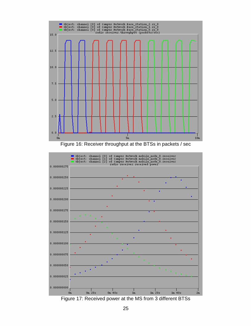
5.3 Simulation 3: In this scenario, there are three base stations and a mobile station (figure 15). The mobile station moves from one base station to another. Therefore, at the beginning of the simulation, the mobile station is attached to the first base station and when it ends, the mobile station is attached to the third base station. The mobile station is performing cell update twice in this scenario (from base station 1 to base station 2 and from base station 2 to base station 3).
Figure 15: Scenario of simulation 3
In this simulation scenario the throughput at the three base stations is collected. The throughput graph (figure 16) shows that at a time only the base station where the mobile resides on receives the data. When the mobile performs a cell update because the signal from another BTS has a higher power (figure 17), it selects the corresponding base station and sets the new transmitter frequency accordingly. This simulation shows that the implementation of the cell update procedure was successful.
25
Figure 16: Receiver throughput at the BTSs in packets / sec
Figure 17: Received power at the MS from 3 different BTSs

26
5.4 Simulation 4: This simulation addresses the task frequency / capacity planning, timeslot allocation and sharing of them by the MSs. A scenario with ten and another scenario with eleven MSs (figure 18) were created.
Figure 18: Simulation scenario 4 with 11 MSs
The speeds of the wired links in the model were set to 171,200 kbps to simulate a case that represents all MS sharing all timeslots on one frequency. The speed of the wireless connection remains unchanged from the former model (because there is no MAC layer for allocation and sharing of the timeslots). Throughput between the BTS and the BSC (figure 19), the end-to-end delay to the sink (figure 21) and the queue size in the uplink buffer of the BTS (figure 20) are measured. The MS send voice-over-IP data with a constant bit rate at 16,100 kbps.

27
Figure 19: Throughput between BTS and BSC in kbps
Figure 20: Queue sizes in the BTS

28
Figure 21: End-to-end delay from the MS to the sink
For ten MSs the end-to-end-delay and the queue size are constant, the throughput is just below the supported 171,200 kbps. The calculated traffic is 10 * 16,100 kbps = 161,100 kbps. As seen in the diagram the queue size increases constantly in the second scenario with eleven MSs, therefore the end-to-end delay increases too. The overall traffic that the MSs are trying to send is 177,100 kbps, the channel does not provide enough capacity for eleven MSs. One channel provides only enough capacity for up to ten MS which want to send voice-over-IP traffic at the desired rate.

29
6. Future work:
To make the model more realistic the following things can be done:
• The MAC / RLC layer with timeslots and allocations has to be implemented. As a result of that the model will also support more users and a larger scenario can be created. The link speeds in the model have to be recalculated and the propagation speed has to be changed to get realistic results.
• Cell identifiers, routing areas, local areas (this will also enable multiple
BSCs) and the standby state are necessary to enable paging of MSs. In reality the SGSN knows only the routing area of a MS in the standby state and therefore the SGSN has to page it to get the cell identifier of the cell where the MS camps on in order to send downlink traffic to it.
• More realistic traffic like busty web traffic (also in the downlink direction)
has to be added. Different multislot classes to simulate MSs with various capabilities and applications should be introduced.
• The implementation of BSSGP will provide flow control.
7. Discussion and Conclusions:
This paper described technical details of the GPRS network and how they were implemented and added to the existing GPRS OPNET model [11]. Wireless links and a BSC with routing algorithm were introduced which enabled multiple BTS support. The power monitor in MS enables the cell update scenario which was implemented in the network independent version. Various simulations, calculations have been performed to verify the implementations. Several aspects and problems of the real network and the model have been addressed were explained in this report. To get more accurate results the model can be further enhanced (e. g. introduce cell identifiers and use them for the routing). The OPNET GPRS model provides a useful tool for performance evaluations and GPRS network planning.

30
8. References
[1]Gunnar Heine, Holger Sagkob, GPRS Gateway to Third Generation Mobile Networks, Artech House, 2003, ISBN 1-58053-159-8
[2]Jukka Lempiainen, Matti Manninen, Radio Interface System Planning for GSM/GPRS/UMTS, Kluwer Academic Publishers, 2001, ISBN 0-7923-7516-5
[3]Emmanuel Seurre, Patrick Savelli, Pierre-Jean Pietri, GPRS for Mobile Internet, Artech House, 2003, ISBN 1-58053-600-X
[4]Ricky Ng, Ljiljana Trajkovic, "Simulation of General Packet Radio,Service Network", OPNETWORK 2002, Washington, DC, Aug. 2002
[5]Mikael Johansson, "Simulation of Logical Link Layer in GPRS", Simon Fraser University, Burnaby, Spring 2003
[6]Digital cellular telecommunications system (Phase 2+), General Packet Radio Service (GPRS) Service description, Stage 2 (3GPP TS 03.60 version 7.9.0 Release 1998)
[7]Christoffer Andersson, GPRS and 3G Wireless Applications: Professional Developer's Guide, John Wiley & Sons, 2001, ISBN 04714140580
[8]General Packet Radio Service (GPRS), External network assisted cell change (NACC), 3GPP TR 44.901 version 5.1.0 Release 5
[9]http://www.gsmworld.com/technology/gprs/intro.shtml (last accessed Dec 7, 2003)
[10]V. Vukadinovic and Lj. Trajkovic, ”OPNET implementation of the Mobile Application Part protocol,” OPNETWORK 2003, Washington, DC, Aug. 2003
[11]Paulman Chan, “GPRS Project Report”, Simon Fraser University, Burnaby, August 30th, 2003

31
Appendix A, Frequency usage:
Uplink frequencies (MS to BTS)Basestation 1 2 3 4 5 6Channel1 (BCCH) 1850.2 1860.2 1870.2 1880.2 1890.2 1900.2
2 1850.8 1860.8 1870.8 1880.8 1890.8 1900.83 1851.4 1861.4 1871.4 1881.4 1891.4 1901.44 1852 1862 1872 1882 1892 19025 1852.6 1862.6 1872.6 1882.6 1892.6 1902.66 1853.2 1863.2 1873.2 1883.2 1893.2 1903.27 1853.8 1863.8 1873.8 1883.8 1893.8 1903.88 1854.4 1864.4 1874.4 1884.4 1894.4 1904.49 1855 1865 1875 1885 1895 1905
10 1855.6 1865.6 1875.6 1885.6 1895.6 1905.611 1856.2 1866.2 1876.2 1886.2 1896.2 1906.212 1856.8 1866.8 1876.8 1886.8 1896.8 1906.813 1857.4 1867.4 1877.4 1887.4 1897.4 1907.414 1858 1868 1878 1888 1898 190815 1858.6 1868.6 1878.6 1888.6 1898.6 1908.616 1859.2 1869.2 1879.2 1889.2 1899.2 1909.2
Downlink frequencies (BTS to MS)Basestation 1 2 3 4 5 6Channel1 (BCCH) 1930.2 1940.2 1950.2 1960.2 1970.2 1980.2
2 1930.8 1940.8 1950.8 1960.8 1970.8 1980.83 1931.4 1941.4 1951.4 1961.4 1971.4 1981.44 1932 1942 1952 1962 1972 19825 1932.6 1942.6 1952.6 1962.6 1972.6 1982.66 1933.2 1943.2 1953.2 1963.2 1973.2 1983.27 1933.8 1943.8 1953.8 1963.8 1973.8 1983.88 1934.4 1944.4 1954.4 1964.4 1974.4 1984.49 1935 1945 1955 1965 1975 1985
10 1935.6 1945.6 1955.6 1965.6 1975.6 1985.611 1936.2 1946.2 1956.2 1966.2 1976.2 1986.212 1936.8 1946.8 1956.8 1966.8 1976.8 1986.813 1937.4 1947.4 1957.4 1967.4 1977.4 1987.414 1938 1948 1958 1968 1978 198815 1938.6 1948.6 1958.6 1968.6 1978.6 1988.616 1939.2 1949.2 1959.2 1969.2 1979.2 1989.2
Table 3: Frequency table for the MSs and BTSs of the GPRS OPNET model: