NASA/TM-2019-104606/Vol. 53

Technical Report Series on Global Modeling and Data Assimilation, Volume 53 Randal D. Koster, Editor

Ensemble Generation Strategies Employed in the GMAO GEOS-S2S Forecast System

Siegfried Schubert, Anna Borovikov, Young-Kwon Lim, and Andrea Molod

November 2019

NASA STI Program ... in Profile

Since its founding, NASA has been dedicated

to the advancement of aeronautics and space

science. The NASA scientific and technical

information (STI) program plays a key part in

helping NASA maintain this important role.

The NASA STI program operates under the

auspices of the Agency Chief Information Officer.

It collects, organizes, provides for archiving, and

disseminates NASA’s STI. The NASA STI

program provides access to the NTRS Registered

and its public interface, the NASA Technical

Reports Server, thus providing one of the largest

collections of aeronautical and space science STI

in the world. Results are published in both non-

NASA channels and by NASA in the NASA STI

Report Series, which includes the following report

types:

TECHNICAL PUBLICATION. Reports of

completed research or a major significant

phase of research that present the results of

NASA Programs and include extensive data

or theoretical analysis. Includes compila-

tions of significant scientific and technical

data and information deemed to be of

continuing reference value. NASA counter-

part of peer-reviewed formal professional

papers but has less stringent limitations on

manuscript length and extent of graphic

presentations.

TECHNICAL MEMORANDUM.

Scientific and technical findings that are

preliminary or of specialized interest,

e.g., quick release reports, working

papers, and bibliographies that contain

minimal annotation. Does not contain

extensive analysis.

CONTRACTOR REPORT. Scientific and

technical findings by NASA-sponsored

contractors and grantees.

CONFERENCE PUBLICATION.

Collected papers from scientific and

technical conferences, symposia, seminars,

or other meetings sponsored or

co-sponsored by NASA.

SPECIAL PUBLICATION. Scientific,

technical, or historical information from

NASA programs, projects, and missions,

often concerned with subjects having

substantial public interest.

TECHNICAL TRANSLATION.

English-language translations of foreign

scientific and technical material pertinent to

NASA’s mission.

Specialized services also include organizing

and publishing research results, distributing

specialized research announcements and

feeds, providing information desk and personal

search support, and enabling data exchange

services.

For more information about the NASA STI

program, see the following:

Access the NASA STI program home page

at http://www.sti.nasa.gov

E-mail your question to help@sti.nasa.gov

Phone the NASA STI Information Desk at

757-864-9658

Write to:

NASA STI Information Desk

Mail Stop 148

NASA Langley Research Center

Hampton, VA 23681-2199

Technical Report Series on Global Modeling and Data Assimilation, Volume 53 Randal D. Koster, Editor

Ensemble Generation Strategies Employed in the GMAO GEOS-S2S Forecast System

Siegfried Schubert Science Systems and Applications, Inc., Lanham, MD

Anna BorovikovScience Systems and Applications, Inc., Lanham, MD

Young-Kwon LimI. M. Systems Group, Inc., College Park, MD

Andrea MolodNASA Goddard Space Flight Center, Greenbelt, MD

National Aeronautics and Space Administration

Goddard Space Flight Center Greenbelt, Maryland 20771

November 2019

NASA/TM-2019-104606/Vol. 53

Notice for Copyrighted InformationThis manuscript has been authored by employees of Science Systems and Applications, Inc., I. M. Systems Group, Inc., with the National Aeronautics and Space Administration. The United States Government has a non-exclusive,

irrevocable, worldwide license to prepare derivative works, publish, or reproduce this manuscript, and allow others to do so, for United States Government purposes. Any publisher accepting this manuscript for publication acknowledges that the United States Government retains such a license in any published form of this manuscript. All other rights are retained by the copyright owner.

Trade names and trademarks are used in this report for identification only. Their usage does not constitute an official endorsement, either expressed or implied, by the National Aeronautics and Space Administration.

Level of Review: This material has been technically reviewed by technical management.

NASA STI ProgramMail Stop 148 NASA’s Langley Research Center Hampton, VA 23681-2199

National Technical Information Service 5285 Port Royal RoadSpringfield, VA 22161703-605-6000

Available from

1

TableofContents

Executive Summary ..................................................................................................................... 3

1.0 Introduction ............................................................................................................................ 7

2.0 The GEOS S2S-1 and S2S-2 Prediction Systems ............................................................... 10

2.1 Ensemble Characteristics ......................................................................................... 12

2.2 Lessons Learned ........................................................................................................ 21

3.0 Ensemble Strategy for the Next System (GEOS S2S-3) .................................................... 23

3.1 The Ensemble Perturbations ..................................................................................... 24

3.1.1 Scaling ....................................................................................................... 24

3.1.2 Spatial structures ........................................................................................ 29

3.2 Sub-setting the Ensemble at Long Leads ................................................................ 37

3.3 Some Initial Tests ...................................................................................................... 39

3.3.1 Perturbation strategy ................................................................................. 41

3.3.2 Ensemble size .............................................................................................. 44

3.3.3 Impact of Stratification .............................................................................. 46

4.0 Summary and Conclusions ................................................................................................. 51

Acknowledgements ..................................................................................................................... 55

References ................................................................................................................................... 57

Previous Volumes ....................................................................................................................... 63

2

3

Executive Summary

This report begins with an assessment of the ensemble characteristics of the current NASA

GMAO GEOS subseasonal to seasonal forecast system (GEOS-S2S-2), with the previous

version (GEOS-S2S-1) serving as a benchmark. The results show that S2S-2 has substantially

increased dispersion in the SST ensemble forecasts compared with S2S-1, producing ensemble

uncertainties in Niño3.4 predictions that are more in line with the actual forecast errors, though

S2S-2 appears to be over-dispersive at some of the longest forecast leads. Furthermore, these

changes in ensemble dispersion appear to reflect changes in the model’s climate variability

rather than any changes in the method of initializing the ensemble members, with the S2S-2

model exhibiting more realistic (increased) subseasonal SST variability, though excessive

interannual (ENSO) variability. It is only at the shorter forecast leads (1-2 months) that S2S-2

still appears to be somewhat under-dispersive.

We next look ahead to improving the ensemble characteristics of the next system (S2S-3) with

an added focus on the sub-seasonal forecast problem. Limited tests of the relative advantages of

time- lagged and burst approaches to ensemble generation showed considerable year to year

variability in the results, with the long lead (beyond 3 months or so) ensemble spread of ENSO

SST indices showing little sensitivity to the actual method of generating the initial uncertainty.

At shorter leads (1-2 months) the under-dispersive nature of the ENSO SST predictions in S2S-2

appears to reflect inadequate (likely too small amplitude) oceanic perturbations, since the

atmospheric perturbations appear ineffective in substantially impacting the SST uncertainty at

such short forecast leads. A statistical analysis of our current approach to generating

perturbations (produced as scaled differences between two analysis states five days apart) shows

4

that, 1) a rich array of physically realistic perturbations (spatial structures) can be obtained for

both the atmosphere and ocean by varying the separation time between the analysis states, 2) the

leading structures of the difference fields have some correspondence with the fastest growing

modes determined from a singular value decomposition of the model’s linear propagator, and 3)

the amplitude of the unscaled difference perturbations is a function of the separation and, as

such, the scale factors should account for the temporal autocorrelation of the fields in question.

Based on the above results, we recommend a strategy for ensemble forecasting for our next

system (S2S-3) that is overall similar to our current approach, in that the strategy employs a

combination of time-lagged and burst ensemble members. A key difference is that, for the burst

mode, we recommend introducing perturbations based on a range of different time lags. This

methodology, referred to as a Synchronized Multiple Time-lagged (SMT) approach to generating

perturbations, injects uncertainty (at a specified time) into a number of key atmospheric and

oceanic modes of variability believed to have a significant impact on the early stages (1-2

months) of forecast error growth. Furthermore, while recognizing the importance of large

ensembles for obtaining reliable estimates of various ensemble forecast statistics (e.g., reliability,

consistency), our assessment of the forecast skill of some of the leading modes of subseasonal

atmospheric variability (e.g., the North Atlantic Oscillation (NAO), the Pacific/North American

(PNA) pattern and the Arctic Oscillation (AO)) indicates that we have little to gain in terms of

skill by increasing the ensemble size much beyond 30 or so. Finally, current computational

resource limitations and timeliness constraints (e.g., for delivery of the forecasts to NMME)

require that we reduce the forecast ensemble size after about 2 months lead time, and we outline

5

a strategy for doing that based on a stratified sampling of the early larger ensemble that accounts

for the emerging directions of error growth. Initial subsampling tests show promising results.

6

7

1. Introduction

Weather and climate prediction are fundamentally probabilistic problems. Efforts to predict the

evolution of the various properties of the underlying probability distribution typically involve

running ensembles of forecasts. While much of the focus of ensemble forecasting has been on

providing improved estimates of the mean (typically used to assess forecast skill), there has also

been considerable effort expended in recent years on improving the estimates of the forecast

uncertainty (the ensemble spread) and related probabilistic measures of forecast quality such as

reliability and consistency (e.g., Jolliffe and Stephenson 2003; Atger 2004; Sansom et al. 2016).

An important outstanding issue in ensemble short-term climate (subseasonal to seasonal)

prediction concerns the best approach to introducing uncertainty in the initial conditions (e.g.,

Vialard et al, 2005). While ideally the uncertainty should reflect the actual errors of the

analyzed initial state, these are typically not well known, and many efforts focus instead on

ensuring that any perturbations that are introduced in the initial conditions project onto the

fastest growing disturbances (e.g., Yang et al. 2006; Magnusson et al. 2008). This focus in part

reflects the fact that many current prediction systems appear to be under-dispersive (ensemble

spread is smaller than actual forecast errors would suggest), but it is also a testament to how far

we still have to go to produce accurate estimates of uncertainties in our analyses of all the

relevant components of the climate system (atmosphere, ocean, land, etc.).

With that in mind, a number of different approaches have been used to generate initial

perturbations to account for initial condition uncertainty. These include the use of time lags

where the perturbations are introduced implicitly by synchronizing the validation time of

8

forecasts initialized at different times in the past (e.g., Dalcher et al. 1988; DelSole et al. 2017),

projections onto both dynamical (e.g., Magnusson et al. 2008) and empirical (e.g., Ham et al.

2012) estimates of the leading singular vectors, and breeding (e.g., Toth and Kalnay 1997; Yang

et al. 2006; Baehr and Piontek 2014). It is important to note that there are other sources of

uncertainties in the forecasts that are tied to model errors. In fact, the lack of progress made in

improving the dispersion characteristics of some models has suggested a need to introduce

additional uncertainty into the model equations. In particular, there has been some success in

dealing with model uncertainty through the introduction of stochastic physics (e.g., Weisheimer

et al. 2014) and the use of multiple models (e.g., Doblas-Reyes et al. 2010).

While a number of studies have attempted to compare the various approaches to addressing

initial condition uncertainty (e.g., Vialard et al. 2005; Magnusson et al. 2008; Andrejczuk et al.

2016), it is unclear to what extent the results are dependent on the given model/forecast system

being studied and/or the metric being used to assess the impact. Nevertheless, we can try to

summarize some general characteristics (drawbacks and advantages) of the above approaches.

These are as follows:

1) Time lagged (typically referred to as lagged-average): relatively easy to implement;

generally requires some delay in producing forecasts depending on lag; there is no direct

control over the size of perturbations (longer lags have larger “perturbations”, see

9

however DelSole et al. 2017 on assigning weights to the lagged ensemble members);

“burst”1 mode is not an option.

2) Dynamical singular vectors: identifies the fastest growing modes (deals with errors

of the day – flow dependence); requires linearized version of the GCM (usually requires

some simplification of the model including the physics); not clear that errors in low

frequencies (important at subseasonal, seasonal, and longer timescales) are well

represented.

3) Breeding: identifies “errors of the day” using the full GCM to grow errors; not clear

that growing errors that evolve spatially over the breeding time are well represented;

requires substantial additional computing for the breeding.

4) Empirical singular vectors: does not require linearized version of model; however,

requires a long history of forecasts to estimate linear operator and does require

substantial simplification (reduction in degrees of freedom) to reduce the number of

parameters to estimate; errors are associated with climatological conditions (not errors

of the day – there is no flow dependence).

In the following, building upon our experience in generating routine subseasonal and seasonal

forecasts with the GEOS S2S forecast system as part of our national and international

commitments to improving short term climate predictions, we outline our plans for ensemble

generation, employing some of the approaches summarized above. In Section 2 we review the

ensemble characteristics of our current system (S2S-2, Molod et al. 2019) with the previous

1 By “burst” mode we refer to the ability to generate multiple ensemble members at a fixed initial time, rather than having to rely on having different initial times to build up an ensemble as is the case for lagged-average forecasts.

10

version (S2S-1, Borovikov et al. 2017) serving as a baseline for comparison. In Section 3, we

address the ensemble strategies to be employed in our next system (S2S-3). Staying with the

same overall strategy of employing perturbations using both the time-lagged approach and time

differences (where perturbations are determined from the differences between two nearby

analysis states), we look (in Section 3.1) in some detail at the nature of those latter (time-

difference) perturbations. Here we focus in particular on how the character of the perturbations

changes with a change in the separation time between the two nearby analysis states. In

addition, a stratified sampling approach to sub-setting ensemble members at some

predetermined lead time is described (Section 3.2) that ensures that the leading directions (in

phase space) of error growth are adequately represented in the sub-sample. Finally, we provide

(in Section 3.3.1) some initial assessment of the relative merits of the time-lagged and

perturbation ensemble generation strategies, while Section 3.3.2 examines the impact on skill of

increasing the ensemble size, and Section 3.3.3 describes the results of some initial tests of our

proposed subsampling approach.

2. The GEOS S2S-1 and S2S-2 Prediction Systems

We begin by comparing various ensemble and climate statistics of the hindcasts/forecasts

produced by the S2S-1 (Borovikov et al. 2017) and S2S-2 (Molod et al. 2019) coupled forecast

systems. These systems have been used by the GMAO over the last few years to produce

forecasts for the National Multi-Model Ensemble (NMME) project (Kirtman et al. 2014) as well

as other national and international projects.

11

The AGCM component of version 1 (described in detail in Borovikov et al. 2017) is Fortuna-2.5

(run at 1° × 1¼° horizontal resolution), while that for version 2 (described in detail in Molod et

al. 2019) is Heracles-5_4_p3 (run at ~½° horizontal resolution). Both AGCMs have 72 hybrid

vertical levels. The OGCM component has been upgraded from Modular Ocean Model version

4 (MOM4) in S2S-1 to MOM5 (Griffies, 2012) in S2S-2, both run at ½ ° horizontal resolution

with a meridional equatorial refinement to 1/4 °, and 40 vertical levels.

S2S-1 was in service from June 2012 through January 2018, and S2S-2 came into production in

December 2017. The S2S-2 forecasts are produced on a fixed set of dates throughout the year;

they are initialized every 5 days (our time-lagged ensemble members), with the date falling

closest to the start of each month including 6 additional ensemble members generated by adding

perturbations to various combinations of the ocean and atmosphere states (our burst ensemble

members). As such, 12 (13 in November) ensemble members are produced each month, though

only 10 are delivered to the NMME (Fig. 1). Hindcasts with the S2S-2 system go back to 1981,

though only 4 (unperturbed) ensemble members (outlined in blue in Fig. 1) were generated each

month. The S2S-1 system used basically the same approach to generating ensemble members

(the same calendar of start dates), though the perturbations to the ocean and atmosphere were

based on a mix of differences between two analyses and perturbations generated by a breeding

approach (Yang et al. 2008), as summarized in Borovikov et al. (2017). Hindcasts for S2S-1

were produced for the period 1982-2012, with forecasts extending from 2013 to 2017; again, a

total of 12 ensemble members were produced for each month for the forecasts and, in this case,

also for the hindcasts.

12

Figure 1: The April 2019 seasonal forecasts produced with the GEOS-S2S-2 system consist of runs initialized every 5 days starting mid-month through the end of the month. Forecasts from the unperturbed initial conditions are run for the 4 start dates (green and orange). The last start date (March 27) includes 6 additional forecasts produced by perturbing the atmosphere and/or the ocean as follows: +/-Datmos, +/-Docean, (+Datmos +Docean), (-Datmos -Docean), where the D is ½ the scaled difference between two analyses that are separated by 5 days. The scaling is such that it produces perturbations in tropical Pacific SST that are a small fraction of the natural variability (10% in terms of standard deviation of the SST in the tropical Pacific region (120°E-90°W, 10°S-10°N)). These 10 forecasts are submitted to NMME.

The comparisons between the S2S-1 and S2S-2 forecast systems presented below are based on

the 4 (unperturbed) ensemble members that the two systems have in common for the 35-year

period (1982-2016). Of course, the limited number of ensemble members available provides a

strong constraint on our ability to provide reliable estimates of a number of ensemble statistics,

such as measures of reliability and consistency, though we believe the results presented here

regarding the ensembles are reasonably robust, especially when considered in a comparative

(rather than absolute) context.

2.1 Ensemble Characteristics

We begin by examining the relationship between the ensemble spread and forecast errors.

Following Barnston et al. (2015) we compare the mean intra-ensemble standard deviation of the

forecasts (x)

13

𝑆𝐷# = &⟨(𝑥 − ⟨𝑥⟩)-⟩............... , (2.1)

with the standard error of the estimate (SEE)2 written as

𝑆𝐸𝐸 = 𝑆𝐷011 − 𝑐𝑜𝑟0⟨#⟩- , (2.2)

where the overbar indicates a long term mean over the 35 years of forecasts/hindcasts (1982-

2016), and the angle brackets denote an ensemble mean. Here 𝑐𝑜𝑟0⟨#⟩is the correlation

between the ensemble mean forecast (⟨𝑥⟩) and the observations (y), given by

𝑐𝑜𝑟0⟨#⟩ =(060.)7⟨#⟩6⟨#⟩....8......................

9:;9:⟨<⟩ , (2.3)

where the standard deviation of the observations (y) is

𝑆𝐷0 = 1(𝑦 − 𝑦.)-........... , (2.4)

and that of the ensemble mean forecasts (⟨𝑥⟩) is

𝑆𝐷⟨#⟩ = 17⟨𝑥⟩ − ⟨𝑥⟩....8-................ . (2.5)

We can then define the ratio

𝑅 = 𝑆𝐷#𝑆𝐸𝐸? , (2.6)

which should ideally be equal to 1 (ensemble spread is equal to the forecast uncertainty). An

under-dispersive model has R values less than 1, while an over-dispersive model has R values

greater than 1.

2 This is the standard error of a simple linear regression in which the predictor is the ensemble mean forecast.

14

Figure 2 shows the intra-ensemble standard deviation (𝑆𝐷#)of the Niño 3.4 index as a function

start month and forecast lead time for both systems. A key difference between the two systems

is the tendency for the variability to saturate earlier in S2S-1 (at about 6 months), whereas the

variance continues to grow in S2S-2 throughout the forecast period.

Figure 2: The intra-ensemble standard deviation of the forecasts of the Niño 3.4 index as a function of start month and forecast lead time for S2S-1 (left) and S2S-2 (right). Results are based on four ensemble members for the forecasts/hindcasts spanning the period 1982-2016.

This is shown more clearly in Fig. 3 (left panels). The S2S-1 forecasts initialized in summer and

early fall, in particular, show clear evidence of saturation (at values of 0.3-0.4 °C) at about 6

months lead time, whereas the S2S-2 ensemble spread continues to grow out to the end of the 9-

month forecast period. Fig. 3 (right panels) shows that the increased ensemble spread in S2S-2

is not limited to Niño3.4 SST but also holds for the SST in most other regions of the globe.

15

Figure 3: Left panels: The evolution of the intra-ensemble standard deviation (𝑆𝐷#) of the Niño3.4 index for different initial start dates (top is for Jun-Sep, and bottom is for Dec–Mar). The solid lines are for S2S-2 and the dashed lines are for S2S-1. The black lines are the square root of the variances averaged over each of the 4 months. The right panels show the average of the SST 𝑆𝐷# for lead 6-month forecasts initialized on June, July, August and September (verifying Dec, Jan, Feb, Mar, respectively). Top panel is for the S2S-1 system and the middle panel is for the S2S-2 system. The bottom panel is the difference. Units are °C. Results are based on four ensemble members for forecasts/hindcasts spanning the period 1982-2016.

Figure 4 shows the skill of the Niño 3.4 forecasts (𝑐𝑜𝑟0⟨#⟩). Taking a correlation of 0.5 as a

rough cutoff for skillful forecasts we see that, with the exception of the forecasts initialized in

January, both systems remain skillful out to 9 months. Nevertheless, S2S-2 is overall more

skillful, especially for forecasts initialized in boreal summer (though it is somewhat less skillful

16

Figure 4: The correlation between the ensemble mean forecast (⟨𝑥⟩) and the observations (y) for the Niño 3.4 index as a function start month and forecast lead time for S2S-1 (left) and S2S-2 (right). Results are based on four ensemble members for forecasts/hindcasts spanning the period 1982-2016.

for forecasts initialized in early spring). These results are reflected in the standard errors of the

estimate (SEE) shown in Figure 5, with smaller values of SEE for S2S-2 clearly evident for

forecasts initialized during boreal summer.

17

Figure 5: The standard error of the estimate, SEE (see text), for the Niño 3.4 index as a function start month and forecast lead time for S2S-1 (left) and S2S-2 (right). Results are based on four ensemble members for forecasts/hindcasts spanning the period 1982-2016.

The extent to which the ensemble spread of the Niño 3.4 forecasts is a reliable indicator of

forecast uncertainty is measured by the ratio R (Fig. 6). This figure shows that S2S-1 does

indeed tend to be under-dispersive, which is consistent with the finding of Barnston et al.

(2015), especially early in the forecasts. In contrast, S2S-2 is if anything over-dispersive,

especially at long leads for forecasts initialized in boreal summer and early winter. Only at very

short leads (1-2 months) is S2S-2 still somewhat under-dispersive.

18

Figure 6: The ratio R (see text) for the Niño 3.4 index as a function of start month and forecast lead time for the S2S-1 system (left) and the S2S-2 system (right). Results are based on four ensemble members for forecasts/hindcasts spanning the period 1982-2016.

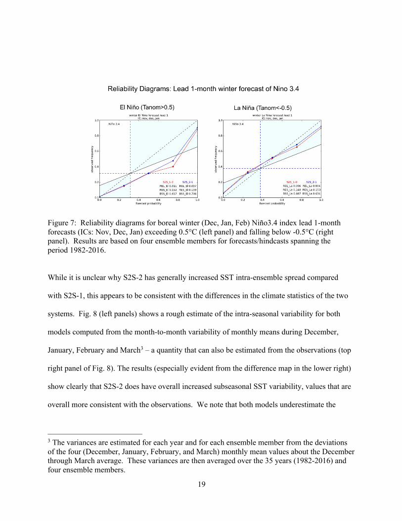
This is reflected in the reliability diagrams in Fig. 7. The lead-1 Niño 3.4 forecasts for both

systems tend to be overconfident, especially in predicting El Niño events, consistent with the

under-dispersive nature of the forecasts at this lead.

19

Figure 7: Reliability diagrams for boreal winter (Dec, Jan, Feb) Niño3.4 index lead 1-month forecasts (ICs: Nov, Dec, Jan) exceeding 0.5°C (left panel) and falling below -0.5°C (right panel). Results are based on four ensemble members for forecasts/hindcasts spanning the period 1982-2016.

While it is unclear why S2S-2 has generally increased SST intra-ensemble spread compared

with S2S-1, this appears to be consistent with the differences in the climate statistics of the two

systems. Fig. 8 (left panels) shows a rough estimate of the intra-seasonal variability for both

models computed from the month-to-month variability of monthly means during December,

January, February and March3 – a quantity that can also be estimated from the observations (top

right panel of Fig. 8). The results (especially evident from the difference map in the lower right)

show clearly that S2S-2 does have overall increased subseasonal SST variability, values that are

overall more consistent with the observations. We note that both models underestimate the

3 The variances are estimated for each year and for each ensemble member from the deviations of the four (December, January, February, and March) monthly mean values about the December through March average. These variances are then averaged over the 35 years (1982-2016) and four ensemble members.

20

variability in the Atlantic. Nevertheless, this overall increase in subseasonal climate variability

would presumably act to increase the intra-ensemble variability in S2S-2.

Figure 8: The intraseasonal SST variability STD (the standard deviation as defined in the text) based on the four months DJFM. The top left panel is for S2S-1 and the bottom left is for S2S-2. The difference is in the bottom right, and the results for the observations are in the top right panel. Units are °C. For the model results the predictions for December, January, February, and March are all from the June initializations. Results are based on four ensemble members for forecasts/hindcasts spanning the period 1982-2016.

Fig. 9 shows the interannual variability for the two systems for the December-March mean SST.

Compared with the observations (top right panel of Fig. 9), we see that both models tend to over-

estimate the tropical Pacific variability (presumably associated with ENSO), though the

overestimate is especially large for S2S-2. It is very likely that this contributes to the over-

dispersive nature of the S2S-2 ensemble forecasts of Niño 3.4 at long leads (Fig. 6). Both

models also overestimate the variability in the western-boundary current regions of the Kuroshio

Current and Gulf Stream. The S2S-2 model has greater interannual SST variability throughout

most of the globe, but particularly in the tropical and South Pacific Ocean (lower right panel of

21

Fig. 9), where it exhibits variability that is considerably larger than that found in the

observations.

Figure 9: The interannual SST variability (STD) based on the mean of the four months DJFM. The top left panel is for S2S-1 and the bottom left is for S2S-2. The difference is in the bottom right, and the results for the observations are in the top right panel. Units are °C. For the model results the predictions for December through March were all initialized in June. Results are based on four ensemble members for forecasts/hindcasts spanning the period 1982-2016.

2.4 Lessons Learned

The key results of our comparison of the ensemble characteristics of the old (S2S-1) and new

(S2S-2) forecast systems are as follows:

• While the results are based on a small ensemble size and limited to SST, all indications

are that the new system has increased dispersion (intra-ensemble spread) compared to

the old system, which is known to be under-dispersive (e.g., Barnston et al. 2015; see

also Fig. 6 above). We note that the DJFM intra-seasonal SST climate variability

appears to be more realistic (greater) in the new model, consistent with the increased

dispersion in the new system.

22

• The new system appears to be over-dispersive in Niño3.4 at long leads, especially for

forecasts verifying in spring. This is likely linked to excessive interannual SST climate

variability in the new model, especially over the tropical Pacific where it is linked to

excessive ENSO variability (Chang et al. 2019)

• The new system tends to be slightly under-dispersive at short (1-2 months) leads, though

it is still better than the old system in this regard. The underestimated dispersion is

perhaps an indication that the initial SST perturbations are too small or don’t project

sufficiently on the growing modes.

• The new system has greater skill for most leads and start dates in predicting Niño3.4,

with spring start dates being the main exception.

Ruling out any differences in how the two sets of hindcasts/forecasts were initialized (both were

initialized from the same set of 4 start dates each month), it appears that the differences in the

SST dispersion characteristics between S2S-1 and S2S-2 are the result of model changes that

acted to increase the model’s climate variability. In particular, the S2S-2 model appears to have

greater overall SST climate variability at both subseasonal and interannual time scales, and this

is presumably the main driver of the greater ensemble spread in the S2S-2 system, especially at

the longer leads. On the other hand, both systems are under-dispersive at short leads (1-2

months), indicating that we need to consider enhancing/changing the perturbations to more

directly impact the SST in the early stages of the forecasts. In fact, a greater focus on the early

ensemble spread is also motivated by our effort to more seamlessly incorporate subseasonal

forecasts into the GEOS S2S-3 system, reflecting the increased national and international

emphasis placed on improving subseasonal forecasts (Pegion et al. 2019).

23

3. Ensemble Strategy for the Next System (GEOS S2S-3)

It is reasonable to assume that we will continue to use a strategy for ensemble generation that is

not too different from our current strategy – with ensemble members produced by a

combination of time-lagged and burst approaches. This reflects a certain level of pragmatism

since it would involve minimal changes to the way we currently operate. Nevertheless, it is a

strategy which allows us to initialize forecasts frequently enough (every 5 days) to address

subseasonal problems, while at the same time generating somewhat larger ensembles in burst

mode on a monthly basis to allow a more controlled assessment of the impact of initial errors on

seasonal forecasts. The burst approach also allows for future substantial increases in the

number of ensemble members without requiring the introduction of further time lags.

Given this basic framework for ensemble generation, we next (Section 3.1) look in more detail

at the characteristics of the perturbations generated as scaled differences between two analyses,

with an eye towards improving the relevance of the perturbations to the subseasonal forecast

problem. Section 3.2 outlines a strategy for sub-setting the ensemble after a specified forecast

lead time, with the understanding that resource limitations will require the longest lead forecasts

to be run with fewer ensemble members. Some initial tests of the ensemble generation

strategies, including an assessment of the impact of ensemble size on forecast skill and an

example of sub-sampling the forecasts using a stratified sampling approach, are presented in

Section 3.3.

24

3.1 The Ensemble Perturbations

Here we examine the impact of varying the length of the separation between the two

analysis states to produce different types of perturbations. We begin by focusing on how to

scale the perturbations in a way that makes the amplitude independent of the separation. This is

followed by an analysis showing that changing the separation time produces different horizontal

structures of the perturbations (e.g., atmospheric synoptic-scale waves and teleconnections,

oceanic instability waves) that are effectively sampled from a covariance structure that has

eigenvectors similar to (or, under some restrictions, are the same as) the singular vectors of the

relevant linear propagator of the model.

3.1.1 Scaling

The perturbations of a quantity (x) for a particular separation (𝜏, 𝑖𝑛𝑑𝑎𝑦𝑠) are defined as:

∆𝑥H(𝑡) ≡ 𝑥(𝑡 + 𝜏) − 𝑥(𝑡), 𝜏 = 1,2, 3… . 𝑑𝑎𝑦𝑠. (3.1)

It is straightforward to show that the variance of the perturbations (𝑉𝑎𝑟(∆𝑥H))satisfies the

relationship

QRS(∆#T)UVW

= 2(1 − 𝜌(𝜏)), (3.2)

where 𝜎Z- is the climatological variance of the daily data and 𝜌(𝜏) = 𝑐𝑜𝑟𝑟7𝑥(𝑡 + 𝜏), 𝑥(𝑡)8 is the

autocorrelation based on the daily data. One can then define a scaling of the perturbations

∆𝑥H_\Z ≡ 𝛼(𝜏)∆𝑥H, (3.3)

such that 𝛼(𝜏) scales the perturbations to have the same magnitude relative to climatology,

independent of the separation 𝜏. In particular

𝛼^(𝜏) = 𝜖 `271 − 𝜌(𝜏)8ab/-

⁄ , (3.4)

25

where 𝜖 is whatever fraction of the climatological standard deviation one wants the magnitude of

the perturbations to be (say 0.1). We note that at long separations (𝜌(𝜏) → 𝑧𝑒𝑟𝑜), the scaling

factor reduces to 𝜖 2b/-⁄ . Also, it is worth noting that if we assume 𝜌(𝜏) ≈ 𝛽H (the

autocorrelation of a stationary first order autoregressive process, where 𝛽 = 𝜌(1)) then

𝛼j(𝜏) = 𝜖 72(1 − 𝛽H)8b/-⁄ , (3.5)

though making such an assumption, while generally valid for the free atmosphere (e.g., Feldstein

2000), is likely not valid near the surface and, in any event, is not necessary assuming we have

enough data to produce reliable estimates of 𝜌(𝜏).

Figure 10 shows some examples of the scaling factor (with 𝜖 = 0.1) for atmospheric potential

temperature, specific humidity, and the zonal and meridional components of the wind. A key

result is that the values generally decay to the limit of 𝜖 2b/-⁄ = 0.071 after about one week of

separation, consistent with the typical decorrelation time scale of large-scale atmospheric

teleconnections (e.g., Feldstein 2000), though it is noteworthy that the values decay less rapidly

than would be suggested by a first order autoregressive process. The other key result is that the

values are overall rather similar, though there is clearly a longer memory closer to the surface for

the temperature and moisture fields. We take advantage of that fact to produce an average set of

scaling factors that vary only with season and separation as shown in Figure 11.

26

Figure 10: The perturbation scaling factor (𝛼^(𝜏)) for various atmospheric quantities and levels as a function of separation (𝜏) in days. Top left: potential temperature, top right: specific humidity, bottom left: u-wind and bottom right: v-wind. Also shown is 𝛼j(𝜏) which assumes the autocorrelations follow a simple first order autoregressive process. Results are based on a sample of 40 differences taken from ocean data assimilation system (ODAS) restarts during the period OND 2017. See text for details (Section 3.1.1).

27

Figure 11: The overall average atmospheric perturbation scaling factor (𝛼^(𝜏) ) for each season as a function of separation (𝜏) in days. Results are based on a sample of 40 differences taken from ODAS restarts during the period SON 2017. See text for details (Section 3.1.1).

Figure 12 shows the results for the ocean temperature and salinity at various depths. While the

overall time scales for the ocean are clearly longer than they are for the atmosphere, our interest

here is again on short term error growth (though of course our underlying concern is how that

eventually leads to error growth in the longer time scales such as ENSO), and so we again focus

on differences in the ocean state just a few days apart. The results do show somewhat larger

values of the scale factor compared with the atmosphere especially for the 1-day differences,

consistent with the longer ocean time scales. Also, we note that even at the 5-day separation the

correlations have not fully decayed to zero. While there is considerable scatter in the scale

factors at the 1-day separation as a function of depth, in practice we utilize a single averaged set

of scale factors that depend only on the separation (𝜏).

28

Figure 12: The perturbation scaling factor (𝛼^(𝜏) ) for ocean temperature (T) and salinity (S) as a function of separation (𝜏) in days at various depths. Top: for shallow depths (5, 15, 25, 35 meters). Bottom: for deeper depths (55, 105, 205, 950 meters). Results are based on a sample of 40 differences taken from ODAS restarts during the period SON 2017. See text for details (Section 3.1.1).

In the following we provide some clues as to the nature of these perturbations (both in the

atmosphere and ocean) by examining their spatial structures as a function of separation (𝜏).

29

3.1.2 Spatial structures

In this section we examine the spatial structure of the perturbations computed as a difference

between two analysis states. We are particularly interested in how the structures vary as a

function of the separation and whether there is any connection with singular vectors (e.g.,

Magnusson et al. 2008). With that in mind we begin by assuming that the perturbations (which

can be considered as a tendency in time or separation 𝜏) are approximately governed by

∆�⃗�H(𝑡) ≡ �⃗�(𝑡 + 𝜏) − �⃗�(𝑡) ≈ 𝐴H�⃗�(𝑡) , (3.6)

where 𝐴H is an n×n matrix and �⃗� is a n×1 vector representing the daily state (over say the n grid

points) of the climate system. Note that the linear propagator, 𝐴H, depends on the lead time t.

We are interested in the spatial structure of the perturbations ∆�⃗�H(𝑡) as a function of t, so we

need to examine the covariance matrix

𝐷H = ⟨∆�⃗�H(𝑡)∆�⃗�H(𝑡)n⟩, (3.7)

where the angle brackets denote an average over the history4 of perturbations being considered

and the superscript T denotes a matrix transpose. Substituting for ∆�⃗�H(𝑡) from above we obtain:

𝐷H = 𝐴H⟨�⃗�(𝑡)�⃗�(𝑡)n⟩𝐴Hn = 𝐴HΣ𝐴Hn, (3.8)

where

Σ = ⟨�⃗�(𝑡)�⃗�(𝑡)n⟩ (3.9)

4 This could be a long history (over many years) of perturbations, or a recent history of perturbations just prior to the start of the particular forecast in question.

30

is the covariance matrix of the daily data. This shows that our perturbations (to the extent that

they reflect the leading EOFs of 𝐷H) are closely related to the optimal perturbations that would be

obtained from a singular value decomposition of the operator 𝐴H. Recall that the left (evolved)5

singular vectors of 𝐴Hare obtained from the eigenvectors of the matrix 𝐴H𝐴Hn (Strang 2006). If

we assume that Σ = I (ie, our initial conditions �⃗�(𝑡)are uncorrelated white noise in space) we

would be sampling from a covariance matrix that has eigenvectors identical to the left singular

vectors of 𝐴H. In addition, since the eigenvalues of 𝐷H are just the square of the singular values,

we would presumably be sampling preferentially those perturbations with the largest growth

rates.

Of course, in our case, Σ ≠ I, but we can show that if we make the coordinate transformation

�⃗� = Γ6b/-𝐸n�⃗� (3.10)

where Σ = EΓ𝐸n, E is a matrix with columns equal to the eigenvectors of Σ, and Γ is a

diagonal matrix containing the eigenvalues of Σ (also E𝐸n = 𝐼), then the coordinate

transformation renders the new variables 𝑧vuncorrelated in space with unit variance

(⟨𝑍(𝑡)�⃗�(𝑡)n⟩ = 𝐼). We can then write

𝐴H�⃗�(𝑡) = 𝐴HΓ6b/-𝐸n𝑍 ≡ 𝐵H�⃗�(𝑡), (3.11)

5 Here we note that the SVD of 𝐴H = 𝑈H𝑅H𝑉Hn where 𝑅H is a diagonal matrix containing the singular values 𝑟y, and 𝑈H and 𝑉H are orthonormal matrices with the columns consisting of the left and right singular vectors (SVs), respectively. Furthermore, since 𝐴H𝑣y = 𝑟y𝑢|⃗ y, the right (left) singular vectors are also denoted as the initial (final) SVs.

31

so that

𝐷H = 𝐴HΣ𝐴Hn = 𝐵H𝐵Hn, (3.12)

where

𝐵H = 𝐴HΓ6b/-𝐸n. (3.13)

The above shows that the EOFs of 𝐷H are identical to the left singular vectors of the matrix 𝐵H,

which is a transformation of the linear propagator 𝐴H associated with the orthogonalized and

normalized state variables 𝑍. As such, we would expect that the leading EOFs of 𝐷H =

𝐴HΣ𝐴Hnresemble the fastest growing disturbances as determined from a singular value

decomposition of 𝐴H (with some dependence on the prevailing covariance structures as

determined by Σ6), and those leading EOFs would likely change as a function of the separation

since 𝐴H is itself a function of t. This indicates that there is something to be gained by creating

perturbations based on several different values of t, in that it allows us to perturb different modes

of variability that contribute to forecast uncertainty on different time scales and in different

regions of the globe.

As an example, we show in Figure 13 the leading EOFs of the mid-tropospheric potential

temperature 1-day and 5-day differences for September – November. The differences in the

spatial structure of the leading EOFs are clearly different, with the 1-day differences having

6 This quantifies the impact of what was noted earlier regarding the choice of the averaging operator < >. In particular, Σ could be the climatological covariance matrix, or it could itself be time dependent if for example the analysis states used to compute the perturbations are computed from a recent history just before the start of the forecasts, therefore providing something of an “errors of the day” flavor to the EOFs of 𝐷H.

32

much more of a synoptic-scale structure typical of NH middle latitude weather systems, while

the 5-day differences produce larger-scale teleconnection patterns reminiscent of, for example,

the Pacific/North American pattern (PNA, Wallace and Gutzler 1981). The middle panel of

Figure 13 shows that the leading EOFs represent anywhere between about 8% and 13% of the

total global variance of the difference fields.

Figure 13: Typical structures of atmospheric perturbations in middle latitudes for potential temperature at model level 49 (approximately 450mb). The patterns are the two leading EOFS computed from 1-day (left) and 5-day (right) differences of ODAS restarts during the period September-November (SON) 2017. The middle panel shows the fraction of total variance associated with the 20 leading EOFS for t equals 1 day through 5 days.

While the above EOFs naturally isolated the leading structures in the middle latitudes where the

day-to-day variability in temperature is largest, we can also look at what the leading structures

are in the tropics by simply confining the domain of the EOF calculation to the tropical region.

33

Here we are particularly interested in whether any of the EOFs are related to the MJO and, if so,

at what separation (t) that first occurs.

Figure 14 shows the leading EOFs of the tropical zonal wind at 850mb and 200mb (computed as

combined or extended EOFs), for t =1, 5, and 10 days during boreal winter. The 1-day

difference appears to highlight variability in the eastern tropical Pacific. A further analysis of

this mode (not shown) indicates that it is part of an eastward propagating Rossby wave couplet

straddling the equator. At both 5- and 10- days separation the structures are much larger in

scale, with the 10-day separation apparently isolating MJO-like variability as shown in the

bottom right panels of Fig 14. It is noteworthy that very similar results are found for boreal

summer (Fig. 15).

Figure 14: Typical structure of atmospheric perturbations in the tropics for zonal wind at 850mb and 200mb during December, January and February (DJF). The patterns are the leading EOFS computed from 1 day (upper left), 5 day (lower left) and 10 day (upper right) differences. The lower right is the structure associated with the MJO computed as the leading EOF from 850mb and 200mb zonal wind in which longer time-scale components (seasonal and interannual) are removed (e.g., method described in Wheeler and Hendon 2004). Results are based on MERRA-2 for the years 1999-2016.

34

Figure 15: Same as Fig. 14 but for JJA.

We next turn to the ocean. It is unclear what the leading structures of the ocean perturbations

based on such short (e.g., 1, 3, 5 days) time differences should look like (or what their relevance

is to the uncertainties in long lead ENSO forecasts) but it is worth keeping in mind that at 5-days

and longer separations, they should resemble the uncertainties introduced into the SST forecasts

from our use of nearby (5 days apart) time-lagged initial conditions. As an example, we show in

Fig. 16 the leading EOFs of the x-z cross-section of the Pacific equatorial temperature

perturbations extending to a depth of 300m during September-November for 1-day and 10-day

separations. The results show modes in which the variability is to a large extent tied to variations

in the thermocline. At one day separation (upper left panel) the leading EOF has values

generally of the same sign throughout the mixed layer and below, with particularly large

contributions at and just west of the dateline below 100 meters. The correlations with SST

(lower left panel) indicate that this mode is associated with SST variations that are spatially

35

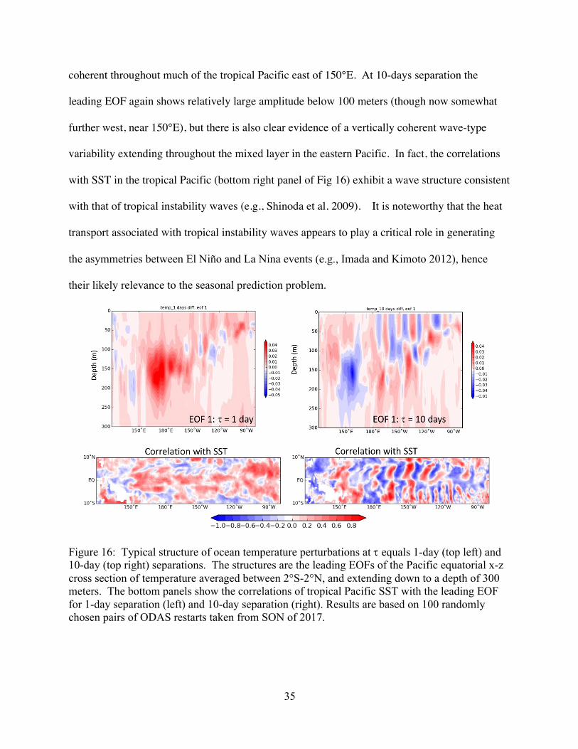
coherent throughout much of the tropical Pacific east of 150°E. At 10-days separation the

leading EOF again shows relatively large amplitude below 100 meters (though now somewhat

further west, near 150°E), but there is also clear evidence of a vertically coherent wave-type

variability extending throughout the mixed layer in the eastern Pacific. In fact, the correlations

with SST in the tropical Pacific (bottom right panel of Fig 16) exhibit a wave structure consistent

with that of tropical instability waves (e.g., Shinoda et al. 2009). It is noteworthy that the heat

transport associated with tropical instability waves appears to play a critical role in generating

the asymmetries between El Niño and La Nina events (e.g., Imada and Kimoto 2012), hence

their likely relevance to the seasonal prediction problem.

Figure 16: Typical structure of ocean temperature perturbations at t equals 1-day (top left) and 10-day (top right) separations. The structures are the leading EOFs of the Pacific equatorial x-z cross section of temperature averaged between 2°S-2°N, and extending down to a depth of 300 meters. The bottom panels show the correlations of tropical Pacific SST with the leading EOF for 1-day separation (left) and 10-day separation (right). Results are based on 100 randomly chosen pairs of ODAS restarts taken from SON of 2017.

36

It is clear from the above results that by varying the separation time (t) between nearby analysis

states we are able to generate a wide array of different types of atmospheric and oceanic

perturbations that represent physically realistic and important modes of variability. In the

atmosphere these include middle latitude baroclinc waves (t=1 day) and teleconnections (t=5

days), as well as (in the tropics) MJO-like variability (t=10 days). In the tropical ocean, the

analogous perturbations appear to be tied to variations in the thermocline, with the longer

separations (e.g., t=10 days) showing clear evidence of tropical instability waves.

In summary, one can think of this approach to generating perturbations as a variant of the

lagged-average approach since we are using the information about the temporal coherence in

nearby analysis states to generate the ensemble members. However, unlike the lagged-average

approach, we are not constrained to go further back in time to generate more

perturbations/ensemble members (and therefore effectively introduce larger and larger

amplitude perturbations). In fact, we have control over the amplitude of the perturbations and,

to some extent, the structure of the perturbations, and we are free to choose the time at which to

introduce the perturbations, allowing ensemble members to be generated in a burst mode. We

shall refer to this as the Synchronized Multiple Time-lagged (SMT) approach to generating

perturbations. Furthermore, the above results suggest that an SMT approach in which the

perturbations are based on separations of at least 1, 3, 5 and 10 days would introduce a

reasonable blend of different physically realizable error structures that are likely to have a

substantial impact on the early (1-2 month) growth of forecast errors in both the ocean and

atmosphere.

37

3.2 Sub-setting the Ensemble at Long Leads

Ideally, we would like to run a large number of ensemble members in order to obtain not only

better estimates of the mean but also the various other probabilistic measures of forecast quality

involving higher order moments. This, of course, has to be weighed against the desire to

increase model resolution and complexity in what is, for practical reasons, always a limited

resource environment (limited computing, limited storage, time constraints for providing near

real time forecasts, etc). In this section, we consider the possibility of running with a reduced

ensemble size for the longer lead forecasts. In particular, we consider here the option of

running with a relatively large number of ensemble members for, say, the first 2 months, and

then selecting a smaller subset to continue out to the longest leads. The question addressed

here is how to optimally select that subset, taking advantage of well-known results on stratified

sampling (Cochran 1963).

The basic idea is that we take advantage of the information about the early error growth that can

be obtained from the relatively large initial ensemble, in a way that ensures the capture, through

proper subsampling, of the leading directions (in phase space) of error growth (e.g., Schubert et

al. 1992). This can be especially important when the ensemble is characterized by more than

one dominant direction of error growth (e.g., the bimodal structure of the underlying probability

density function (PDF) that would be obtained if roughly half of the ensemble members are

tending to El Niño conditions, while the other half are tending to La Nina conditions).

The approach we use assumes that for a quantity y, we have a large ensemble of size N (the

population) that we wish to subsample with n ensemble members, where N>>n. The

38

population of size N is divided into L disjoint strata, where nh (Nh) are the number of members

of the sample (population) in stratum h. Then the optimal sampling strategy (called Neyman

allocation: it is optimal in the sense that it minimizes the variance of the sample mean) consists

of performing random sampling in each stratum where the number of members in each stratum

is chosen according to (Cochran 1963):

~�~= ��9�

∑ ��9��, (3.14)

where

𝑆�- =b

��6b∑ ((𝑦�)v − 𝑌�� )-��v�b (3.15)

is the population variance of y in stratum h, and

𝑌�� = b��∑ (𝑦�)v��v�b (3.16)

is the population mean in stratum h. Another (simpler) sampling strategy is proportional

sampling, wherein each stratum is sampled in proportion to its representation in the population

as given by

~�~= ��

�. (3.17)

While it would seem that Neyman allocation would be the better approach in general, it may be

that proportional allocation would be a reasonable fallback if the population size N is too small

to obtain reliable estimates of the population variances in each stratum. As we shall see

(Section 3.3.3), such an approach (while not optimal) nevertheless produces considerable

improvements over simple random sampling.

39

The success of the above sampling strategies requires that we are able to divide the population

(N) into L strata. One reasonable approach to doing this is to divide the population in a way

that minimizes the average intra-stratum variance (see e.g., Schubert et al. 1992). Algorithms

for this are readily available. The KMEANS clustering algorithm is just one example (Spath

1980). This algorithm requires specifying the number of clusters (L) along with some initial

guess of the cluster distribution, which could in our case be the cluster obtained from the

previous forecast. Given that our population size (N) is likely to be only about 40 and our

sample size (n) about 10, a reasonable number of clusters is likely to be no more than 3 or 4.

We could for example carry out the clustering based on the Niño3.4 index, since it is likely that

beyond two months or so, our focus should be on obtaining the best possible ENSO forecast for

a given sample size. We present an example of such an approach in Section 3.3.3.

3.3. Some Initial Tests

We have carried out a limited number of experiments (Table 1) with the current (GEOS-S2S-2)

system to examine the impacts of various options outlined in the previous sections for

generating and selecting ensemble members. A key issue concerns the relative

advantages/disadvantages of employing a burst versus a lagged-average approach (e.g., Trenary

et al. 2018). The various other issues considered are whether there is a sensitivity to the sign of

the perturbation, the amplitude of the perturbations, and the separate impacts of perturbing the

atmosphere versus the ocean (Section 3.3.1). We also examine, in Section 3.3.2, the impact of

ensemble size on the skill of predicting some of the leading modes of atmospheric subseasonal

variability. Finally, we present in Section 3.3.3 some initial results showing the benefits of

40

stratified sampling. It is important to note that these results are not meant to be a

comprehensive assessment; they merely provide some initial guidance on how to proceed. We

anticipate redoing some of these experiments as the new system (S2S-3) becomes available for

testing.

Table 1: List of experiments carried out with S2S-2 to examine the impact of various burst and lagged-average strategies, as well as the impact of ensemble size, on skill. # ensemble members

Perturbed variables Notes Year Month/Day

40 potential temperature (PT), specific humidity (Q), zonal wind (U), and meridional wind (V)

Atmos. perturbations t = 1, 2, 3, 4, 5 days (8 of each) e = 0.10 (see eq. 3.4 in text)

2005 2006 2009 2010 2015 2017

11/27 & 03/27

40 PT, Q, U, V Atmos. perturbations t = 1, 2, 3, 4, 5 days e = 0.15 (assess sensitivity to e)

2017 11/27

30 the entire state implicit perturbations via time lags initialized each day of the month

2017 Daily Nov & Mar

40 temp, salt, u, v, t_surf, s_surf, u_surf, v_surf,sea_lev, frazil

Ocean perturbations t = 1, 2, 3, 4, 5 days e =0.10

2017 11/27

40

HSKINI, HSKINW, SSKINI, SSKINW, TSKINI, TSKINW

Surface only (saltwater restarts) t = 1, 2, 3, 4, 5 days e =0.10

2017 11/27

41

3.3.1 Perturbation Strategy

Figure 17 shows an example of some of the key results (in terms of ensemble spread of Niño

3.4) for experiments initialized in November of 2017. Comparisons are made with how we

currently produce our forecasts with the S2S-2 system (labeled S2S, see Section 2). Here we

have plotted the S2S-2 results for the 4 lagged forecasts (green) and the 6 burst forecasts (olive)

separately. This shows quite clearly that while the ensemble spread for the first month

(December) is smaller for the burst forecasts (compared to the lagged-forecasts), by the third

month (February) the ensemble spread for the two sets of forecasts is essentially

indistinguishable. Similarly, other burst forecasts (with larger ensembles) involving only

atmospheric perturbations (yellow, 40 members), ocean perturbations (blue, 40 members) and

SST perturbations (purple, 40 members), produce considerably less spread during the first

month, compared to the lagged forecasts (magenta, 30 members- initialized each day during

November). This is not too surprising for the atmospheric perturbations, since it presumably

takes some time for those perturbations to impact the ocean. It does, however, suggest that we

may want to increase the amplitude of the ocean and SST perturbations in order to increase their

early impacts (recall that the S2S-2 system appears to be somewhat under-dispersive at short

leads). The fact that all the strategies appear to produce similar ensemble spread after the third

month or so is consistent with the results of Vialard et al. (2005). There is some suggestion that

the lagged forecasts, while having an initially larger spread, produce an ensemble spread that

grows more slowly than that of the burst forecasts (cf. the magenta and yellow results before

and after February), suggesting a combination of lagged and burst forecasts may be the best

approach for increasing ensemble spread throughout the forecast period.

42

Figure 17 A comparison of various strategies for producing initial ensemble members: impact on ensemble spread shown as box and whisker plots where the whiskers denote the maximum and minimum values and the box has length equal to 2 standard deviations centered on the ensemble mean. Results are for forecasts initialized during November 2017, with the nominal first month of the forecast being December. Here S2S-2 lagged nov results (green) are for the 4 lagged forecasts (initialized 5 days apart) from our production forecasts, while the lagged results (magenta) are based on 30 members- initialized each day during November. See text for details.

The set of predictions for Dec 2015 (Figure 18) is a rather unusual case. The set of 4 hindcasts

from our current (S2S-2) approach (we did not produce burst ensemble members when running

in hindcast mode – that only started in 2017, see Section 2) showed very little if any ensemble

spread out to 6 months lead. This appears to be in part a sampling issue since the 30 member

lagged results do in fact show a systematic increase in spread through the forecast period. This

is also true for the other (burst) approaches, though compared to 2017 the uncertainty does

appear to grow more slowly with forecast lead. While this in itself may be an interesting

predictability issue to investigate further (though this is beyond the scope of the present

43

analysis), it also points to the limitations of having so few (4) ensemble members to address

forecast uncertainty.

Figure 18: A comparison of various strategies for producing initial ensemble members: impact on ensemble spread shown as box and whisker plots where the whiskers denote the maximum and minimum values, and the box has length equal to 2 standard deviations centered on the ensemble mean. Results are for forecasts initialized during November 2015, with the nominal first month of the forecast being December. See text for details.

Other results, not shown here, indicate little impact on the Niño3.4 ensemble spread from

increasing the amplitude of the atmospheric perturbations from 10 to 15% of the climatological

standard deviation. Also, we did not find any systematic differences when comparing the

results for positive and negative atmospheric perturbations. Finally, we note that various

initialization strategies – bursts of atmospheric, ocean, and SST-only perturbations and lagged

ensembles – do not necessarily have uniform (with forecast lead) effect on the SST spread.

This undoubtedly reflects the limited number of cases we have available for study and the fact

that even at 6-month lead the Niño3.4 SST ensemble spread has yet to reach saturation.

44

3.3.2 Ensemble Size

We next turn to an assessment of the impact of ensemble size on forecast skill. As already

mentioned, the S2S-2 forecasts contributed by the GMAO to the NMME consist of 10 ensemble

members (see e.g., Fig. 1). Limiting the ensemble size to 10 was determined by practical

considerations (e.g., computing resources, time constraints for delivering the forecast to

NMME, etc.), and we recognize that this small size is very likely insufficient for properly

estimating the various probabilistic measures of the forecast. It is however unclear what the

optimal size of the forecast ensemble should be, since it presumably depends on the metric that

is used to determine forecast quality (e.g., skill, reliability, consistency), as well as the

underlying predictability of the phenomena (e.g., ENSO, MJO, NAO, etc.) and time scales of

interest.

Here we attempt to provide some guidance for what a more appropriate ensemble size may be,

focusing on forecast skill (in particular the correlation between the ensemble mean forecast and

observations) of some of the leading extratropical modes of variability (PNA, NAO, AO). We

focus on these modes because there is some evidence that a substantial increase in skill in

forecasting them can be obtained by greatly increasing the number of ensemble members well

beyond the 10 or so typically used in seasonal forecasting (Scaife et al. 2014).

The results presented here are preliminary since they are based on only 6 years of forecasts

(2005, 2006, 2009, 2010, 2015, 2017), all initialized on Nov 27. For this purpose we examine

the results of 40 ensemble members (produced by perturbing the atmosphere, see Table 1) for

each year of forecast, though we make use of the fact that we can generate M = N!/[k!(N-k)!]

45

different combinations of size k from the N=40 ensemble members. The results (in this case the

correlations with observations) based on the ensemble means of the M different sets of k

members are averaged to get an average correlation for that ensemble size. At one extreme, if

k=1 then M=40, and we generate 40 correlations from the 40 individual ensemble members,

which we then average into a single value. At the other extreme, if k=40, then we have M=1,

which gives us just 1 correlation value associated with the ensemble mean of 40 members.

Given that we only have 6 years of forecasts, we also combine the results for various ranges of

forecast leads.

Figure 19 shows that at short forecast leads (1-10 days) the skill is already quite high for a

single ensemble member and that the skill saturates at about 5 ensemble members. There is also

some evidence that increasing the ensemble size has the greatest impact on PNA forecasts at

these leads. At longer forecast lead times (11-20 days, and 21-30 days) the overall skill levels

drop as expected, but there is also a gradual increase in skill with increasing number of

ensemble members, though any increase beyond about 30 members is quite marginal. At the

longest lead times (31- 50 days) the skill is quite low (no skill for the AO), and again little

support for increasing the ensemble size much beyond 30 or so.

In summary, these results indicate that much of the overall increase in skill in predicting these

leading extratropical atmospheric modes at subseasonal time scales occurs in going from a

single ensemble member to about 10 ensemble members. Also, the skill largely saturates at

about 30 ensemble members. There is, however, some suggestion that skill continues to

increase slowly for ensemble sizes greater than 30 for the longer forecast leads (beyond 20 days

46

or so), consistent with the Scaife et al. (2014) study which focused on seasonal forecasts of the

NAO.

Figure 19: The impact of ensemble size on skill of the forecasts made with the S2S-2 system for the NAO, PNA and AO indices as measured by the correlations with observations (MERRA-2). The results are based on 40 ensemble members (with perturbed atmospheric conditions) initialized on Nov 27 of the years 2005, 2006, 2009, 2010, 2015, 2017. Results for lead times within the indicated ranges are combined to increase the degrees of freedom. See text for details.

3.3.3 Impact of Stratification

Here we utilize the 5 months-long experimental forecasts initialized in November 2017 (Table

1) to assess our sampling strategy (see Section 3.2). The full 110-member ensemble consists of

30 that are based on lagged initial conditions (runs started each day in Nov 1-30) and 80 that are

initialized on Nov 27 using the burst approach; of the latter, 40 have atmospheric perturbations

47

and another 40 have oceanic perturbations. Given the importance of ENSO at the longer

forecast leads, we focus on the Niño3.4 SST index.

We treat the N=110 ensemble members as our population and wish to choose an optimal7

subsample in the sense that it minimizes the variance of the sample mean (see Section 3.2).

While at this point the choice of the size of our subsample is somewhat arbitrary, we consider

here an n=30-member subsample, since it likely represents a realistic downsizing fraction that

we hope to introduce in practice (with the smaller ensemble being roughly 1/4 the size of the

larger initial ensemble, whatever that may turn out to be).

We consider subsampling after both the first month (Dec 2017) and second month (Jan 2018) of

the forecasts to get some sense of the sensitivity of the stratification to the lead time at which we

do the subsampling. The stratification in each case is based on the daily Niño3.4 values and

employs the KMEANS algorithm to separate the grand ensemble into L clusters (see section

3.2), where we consider values of L = 3, 4, 5, 6, 7 and 10. We select, at random, a sample of

members from each cluster (h), where the size of each sample is proportional to the size of

corresponding population cluster (𝑛� = 𝑛 ���,or the so-called proportional sampling – see

Section 3.2). The monthly 30-member ensemble means obtained from such a sampling strategy

are compared with those obtained by simply taking a sample of 30 members at random from the

7 While (as discussed in Section 3.2) Neyman sampling is optimal, we choose here to do proportional sampling given the overall limited number of ensemble members we have to compute the within-strata population variances.

48

population’s 110 ensemble members. We note that an unbiased estimate of the mean for

stratified sampling is (Cochran 1963):

𝑦\� = ∑ ���𝑦�...�

��b , (3.18)

where

𝑦�... =b~�∑ 𝑦�v~�v�b (3.19)

is the mean of 𝑦 in stratum h. In the case of proportional sampling (3.1.7), we have:

𝑦\� = ∑ ���𝑦�...�

��b = ∑ ~�~𝑦�...�

��b = b~∑ ∑ 𝑦�v

~�v�b

���b , (3.20)

which is simply the average of the n=30 stratified ensemble members.

The key metric we use to assess the value of stratification is the ratio (ℜ) of the variance of the

sample mean obtained from stratification (𝑦\� ) to that obtained from a simple random sampling

of the population (𝑦S� ), namely

ℜ = QRS(0�)....

QRS(0�)...... (3.21)

We compute those variances using a Monte Carlo approach. In particular, given the L

clusters/strata, we randomly sample the strata proportionally (in fact we do this 1000 times with

different random seeds), to obtain 1000 estimates of the sample ensemble mean, from which we

then estimate the variance of the sample mean. Those results are compared with the results

obtained analogously for simple random sampling from the population.

Figure 20 shows, as an example, the results for 5 strata. The individual dashed lines are the

1000 30-member ensemble means computed with the repeated sampling described above. All

the results (whether obtained through stratified or random sampling, during either the first or

49

Figure 20: Ensemble means of forecasted Niño3.4 based on stratified (left panels) and random (right panels) sampling. The top panels are based on choosing the ensemble members from the 1st month of the forecasts (Dec 2017), while the bottom panels are based on choosing them from the second month (Jan 2018). For the left panels, the sampling is done proportionally employing 5 strata/clusters. The population size is 110 while the subsampled ensemble consists of 30 members. The individual lines are the ensemble means, 𝑦,� produced by repeatedly sampling 30 members using a Monte Carlo approach (with 1000 random seeds), sampling randomly from within the strata (left panels) and from the entire population (right panels). The thick solid lines show the mean of the original 110-member ensemble.

second month) show basically the same evolution as the grand mean (thick solid lines). There

are, however, substantial differences in the variance of the ensemble means, as suggested by the

differences in the spread of the 1000 ensemble members. In particular, the initial spread

appears much reduced for the stratified samples (left panels) compared to that for the random

sampling from the full population (right panels). It also appears that the stratification based on

the second month (bottom left panel of Fig. 20) produces reduced spread (variance of the

ensemble means) that extends out to longer forecast leads (cf. top left and bottom left panels of

50

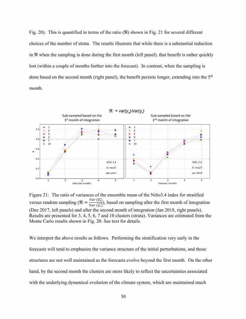
Fig. 20). This is quantified in terms of the ratio (ℜ) shown in Fig. 21 for several different

choices of the number of strata. The results illustrate that while there is a substantial reduction

in ℜ when the sampling is done during the first month (left panel), that benefit is rather quickly

lost (within a couple of months further into the forecast). In contrast, when the sampling is

done based on the second month (right panel), the benefit persists longer, extending into the 5th

month.

Figure 21: The ratio of variances of the ensemble mean of the Niño3.4 index for stratified versus random sampling (ℜ = QRS(0�)....

QRS(0�).....), based on sampling after the first month of integration (Dec 2017, left panels) and after the second month of integration (Jan 2018, right panels). Results are presented for 3, 4, 5, 6, 7 and 10 clusters (strata). Variances are estimated from the Monte Carlo results shown in Fig. 20. See text for details.

We interpret the above results as follows. Performing the stratification very early in the

forecasts will tend to emphasize the variance structure of the initial perturbations, and those

structures are not well maintained as the forecasts evolve beyond the first month. On the other

hand, by the second month the clusters are more likely to reflect the uncertainties associated

with the underlying dynamical evolution of the climate system, which are maintained much

51

longer into the forecast. One final note is that we find rather little benefit from increasing the

number of strata beyond 4 or 5. This is presumably in part a reflection of the limited size (110

members) of our population.

4. Summary and Conclusions

Many models used for short term climate forecasts tend to be under-dispersive in their SST

ensemble forecasts. GEOS S2S-1 (the system first used by the GMAO to provide forecasts to

the NMME project) is no exception, with a history of producing overconfident El Niño

forecasts; for S2S-1, the ensemble spread in the Niño SST indices is small compared to the

actual forecast errors. This changed in 2017 with the introduction of the S2S-2 system. While

our analysis here was based on a limited number of ensemble members, all indications are that

this system has considerably increased dispersion in the SST ensemble forecasts compared with

S2S-1, producing ensemble uncertainties in Niño3.4 predictions that are more in line with the

forecast errors, though S2S-2 appears to be over-dispersive at some of the longest forecast

leads. These changes in ensemble dispersion appear to reflect changes in the model climate

variability rather than any changes in the method of initializing the ensemble members (both

sets of predictions examined here were based on only time-lagged initial states), with the S2S-2

model exhibiting more realistic (increased) subseasonal SST variability, though excessive

interannual (ENSO) variability. It is only at the shorter forecast leads (1-2 months) that the

S2S-2 system still appears to be somewhat under-dispersive.

Looking ahead to our next subseasonal-to-seasonal forecast system (S2S-3), we have examined

in more detail our approaches to generating ensemble members. Currently these are generated

52

using a combination of time-lagged initial conditions (initialized every 5 days on a fixed

calendar) and so-called burst forecasts initialized on the pentad falling closest to the beginning

of the month. For the bursts, the ensemble members are currently generated by adding

perturbations to the analysis state, with the perturbations consisting of scaled differences

between two analysis states separated by 5 days. We analyze here the characteristics of the

perturbations generated in this way, with some focus on how these characteristics vary with the

separation time (t) between the two analysis states used to generate them. The key results are:

1) By varying the time between the two analysis states (from t=1 to 10 days), we are able

to produce perturbations representative of a wide array of what appear to be physically

realistic spatial structures in both the atmosphere and ocean. In fact, an examination of

the leading eigenvectors (EOFs) of the relevant covariance matrices of the difference

fields shows that the perturbations are in effect sampling well-known modes of

variability. In the atmosphere these modes include middle latitude synoptic weather

systems and teleconnections, tropical easterly waves, and MJO-like structures, while in

the ocean these include various fluctuations in the thermocline and tropical Pacific

instability waves.

2) A further analysis of the EOFs associated with the difference fields shows that they are

strongly similar to the fastest growing modes of the linear propagator of the relevant

dynamical system. In fact, under somewhat restrictive conditions, the EOFs of the

difference fields are identical to the left singular vectors of the appropriately linearized

dynamical operator.

3) The amplitude of the unscaled difference perturbations is a function of the separation

(t). Therefore, efforts to provide a consistent amplitude of the perturbations that is

53

independent of t (for example, if it is desirable for all perturbations to have amplitudes

that are a fixed fraction of the climatological variance) must account for the temporal

autocorrelation of the fields in question.

Based on these results, we recommend that for our upcoming S2S-3 forecast system, the

perturbations used for the burst approach should be generated with several different separation

times between the analysis states, an approach we refer to as a Synchronized Multiple Time-

lagged (SMT) approach. This appears to be a viable (relatively simple to implement and

effective) approach to injecting uncertainty into a number of key atmospheric and oceanic

modes of variability believed to have a significant impact on the early stages (1-2 months) of

forecast error growth.

Results of our initial limited tests employing both time-lagged and burst modes with the S2S-2

system varied considerably from one year to the next. Nevertheless, a number of results appear

to be reasonably robust. Focusing on SST, we found that after the first few months all of the

various approaches we tried (lagged, burst, atmosphere-only perturbations, ocean-only

perturbations) produced similar results in terms of the Niño3.4 ensemble spread, consistent with

previous results with other systems (e.g., Vialard et al. 2005). Somewhat greater spread was

seen early on for the lagged ensembles, presumably reflecting the effectively larger initial

perturbations from that approach, with however some evidence of more rapid growth of

ensemble spread for the burst forecasts during the first few months. In addition, we believe that

in order to substantially increase the ensemble spread in Niño3.4 during the first 1-2 months, we

will likely need to increase the amplitude of the perturbations in the ocean given that the

54

atmospheric perturbations appear to be ineffective in impacting the ocean on such short time

scales.

While we have yet to isolate the separate impacts of the different SMT perturbations on the

overall growth of uncertainty (something that will require many more forecasts than are

currently available), we are nevertheless convinced (given their connections to physically

realistic modes of variability) that such perturbations should play an important role, especially

in the growth of uncertainty in the atmosphere during the first month or so of the forecasts (the

subseasonal forecasts). With that in mind, we recommend a combination of lagged and burst

approaches (with burst perturbations computed with separation time scales of 1, 3, 5 and 10

days) as the best way of ensuring that we sweep the widest range of possible error growth

trajectories, especially during the first few months of the forecasts.

Our tests regarding ensemble size focused on assessing improvements in the skill of predicting

some of the leading modes of boreal winter atmospheric variability, particularly the NAO, PNA

and AO. This focus was inspired by the results of Scaife et al. (2014), which suggest that the

skill of predicting the NAO (at seasonal time scales) continues to increase with ensemble size

out to 60 members and beyond. Our results, while not entirely inconsistent with the Scaife et al.

(2014) study, indicate that little is to be gained (in terms of skill) by increasing the ensemble

size much beyond 30 or so, though it should be noted that our focus was on subseasonal time

scales, and we did find some small increase in skill for larger ensemble sizes (beyond 30) at the

longer forecast leads.

55

Finally, anticipating continued computational resource limitations and timeliness constraints

(e.g., for delivery of the forecasts to NMME), we have outlined a strategy for reducing the

forecast ensemble size after a specified lead time (say, 2 months). Based on our initial results,

the strategy, which involves performing a stratified sampling of the early larger ensemble in a

way that accounts for the emerging directions of error growth, shows considerable promise for

reducing the uncertainty in the ensemble mean (compared with simple random sampling) when

the sampling is done after the second month of the forecasts. To some degree, the reduction in

uncertainty appears to be maintained up to 3 months further into the forecasts.

Acknowledgements

We thank Jelena Marshak for running all the experiments. This work benefitted from Amal El

Akkraoui, Eric Hackert, Richard Cullather, Yury Vikhliaev, Robin Kovach, and Bin Zhao

sharing their expertise and helping to brain-storm ideas. This study was supported by NASA

MAP funding under WBS 802678.02.17.01.33.

56

57

References

• Andrejczuk, M., F.C. Cooper, S. Juricke, T.N. Palmer, A. Weisheimer, and L. Zanna,

2016: Oceanic Stochastic Parameterizations in a Seasonal Forecast System. Mon. Wea.

Rev., 144, 1867–1875, https://doi.org/10.1175/MWR-D-15-0245.1

• Atger, F., 2004: Estimation of the reliability of ensemble based probabilistic

forecasts. Quart. J. Roy. Meteor. Soc., 130, 627–646.

• Baehr, J. and R. Piontek, 2014: Ensemble initialization of the oceanic component of a

coupled model through bred vectors at seasonal-to-interannual timescales. Geosci. Model

Dev., 7, 453-461.

• Barnston, A.G., M.K. Tippett, H.M. van den Dool, and D.A. Unger, 2015: Toward an

Improved Multimodel ENSO Prediction. J. Appl. Meteor. Climatol., 54, 1579–1595, DOI

10.1175/JAMC-D-14-0188.1

• Borovikov, A., R. Cullather, R. Kovach, J. Marshak, G. Vernieres, Y. Vikhliaev, B.

Zhao, Z. Li., 2107: GEOS-5 seasonal forecast system. Clim. Dyn.,

https://doi.org/10.1007/s00382-017-3835-2

• Chang, Y., S. Schubert, R. Koster, A. Molod and H. Wang., 2019: Tendency Bias

Correction in Coupled and Uncoupled Global Climate Models with a focus on impacts

over North America. J. Climate, 32, 639–661, 2019. https://doi.org/10.1175/JCLI-D-18-

0598.1

• Cochran, W.G., 1963: Sampling Techniques. John Wiley & Sons, Inc. 413pp.

58

• Dalcher, A., E. Kalnay, and R.N. Hoffman, 1988: Medium Range Lagged Average

Forecasts. Mon. Wea. Rev., 116, 402–416, https://doi.org/10.1175/1520-

0493(1988)116<0402:MRLAF>2.0.CO;2.

• DelSole, T., Trenary, L., and Tippett, M. K., 2017: The Weighted-Average Lagged

Ensemble. Journal of advances in modeling earth systems, 9(7), 2739–2752.

doi:10.1002/2017MS001128.

• Doblas-Reyes, F. J., Deque, M. and Piedelievre, J. P., 2000: Model and multi-model

spread and probabilistic seasonal forecasts in PROVOST, Quart. J. Roy. Meteor. Soc.,

126, 2069 - 2087. 10.1002/qj.49712656705.

• Feldstein, S.B., 2000: The Timescale, Power Spectra, and Climate Noise Properties of

Teleconnection Patterns. J. Climate, 13, 4430–4440, https://doi.org/10.1175/1520-

0442(2000)013<4430:TTPSAC>2.0.CO;2

• Griffies, S., 2012: Elements of the Modular Ocean Model (MOM). http://mdl-mom5.

herokuapp.com/web/docs/project/MOM5_elements.pdf .

• Ham, Y.-G., S. Schubert, and Y. Chang, 2012: “Optimal Initial Perturbations for

Ensemble Prediction of the Madden-Julian Oscillation during Boreal Winter”, J. Climate,

25, 4932–4945, 2012.

• Imada, Y. and M. Kimoto, 2012: Parameterization of Tropical Instability Waves and

Examination of Their Impact on ENSO Characteristics. J. Climate, 25, 4568–

4581,https://doi.org/10.1175/JCLI-D-11-00233.1

59

• Jolliffe, I. T., and D. B. Stephenson, 2003: Forecast Verification. Wiley, 240 pp.

• Kirtman, B.P., D. Min, J.M. Infanti, J.L. Kinter, D.A. Paolino, Q. Zhang, H. van den

Dool, S. Saha, M.P. Mendez, E. Becker, P. Peng, P. Tripp, J. Huang, D.G. DeWitt, M.K.

Tippett, A.G. Barnston, S. Li, A. Rosati, S.D. Schubert, M. Rienecker, M. Suarez, Z.E.

Li, J. Marshak, Y. Lim, J. Tribbia, K. Pegion, W.J. Merryfield, B. Denis, and E.F. Wood,

2014: The North American Multimodel Ensemble: Phase-1 Seasonal-to-Interannual

Prediction; Phase-2 toward Developing Intraseasonal Prediction. Bull. Amer. Meteor.

Soc., 95, 585–601, https://doi.org/10.1175/BAMS-D-12-00050.1

• Magnusson, L., M. Leutbecher, and E. Källén, 2008: Comparison between Singular

Vectors and Breeding Vectors as Initial Perturbations for the ECMWF Ensemble

Prediction System. Mon. Wea. Rev., 136, 4092–4104,

https://doi.org/10.1175/2008MWR2498.1

• Molod, A., E. Hackert, L. C. Andrews, R. M. Kovach, B. Zhao, Z. Li, Y.-K. Lim, A.

Borovikov, G. Vernieres, J. Marshak, R. Koster, J. Carton, R. Cullather, D. Barahona, S.

Schubert, D. Achuthavarier, Y. Vikhliaev, J. L. M. Freire, K. M. Longo, 2019: GEOS-

S2S Version 2: The GMAO high resolution coupled model and assimilation system for

seasonal prediction. Submitted to J. Geophysical Research, 2019.

• Pegion, K., B.P. Kirtman, E. Becker, D.C. Collins, E. LaJoie, R. Burgman, R. Bell, T.

DelSole, D. Min, Y. Zhu, W. Li, E. Sinsky, H. Guan, J. Gottschalck, E.J. Metzger, N.P.

Barton, D. Achuthavarier, J. Marshak, R.D. Koster, H. Lin, N. Gagnon, M. Bell, M.K.

Tippett, A.W. Robertson, S. Sun, S.G. Benjamin, B.W. Green, R. Bleck, and H. Kim,

60

2019: The Subseasonal Experiment (SubX): A multi-model subseasonal prediction

experiment. Bull. Amer. Meteor. Soc., https://doi.org/10.1175/BAMS-D-18-0270.1

• Sansom, P.G., C.A. Ferro, D.B. Stephenson, L. Goddard, and S.J. Mason, 2016: Best

Practices for Postprocessing Ensemble Climate Forecasts. Part I: Selecting Appropriate

Recalibration Methods. J. Climate, 29, 7247–7264, https://doi.org/10.1175/JCLI-D-15-

0868.1

• Scaife, A. A., et al. , 2014: Skillful long-range prediction of European and North

American winters, Geophys. Res. Lett., 41, 2514–2519, doi:10.1002/2014GL059637

• Schubert, S.D., M. Suarez, J-K Schemm, and E. Epstein, 1992: Dynamically Stratified

Monte Carlo Forecasting, Mon. Wea. Rev., 120, 1077-1088.

• Shinoda, T., G.N. Kiladis, and P. E. Roundy, 2009: Statistical representation of equatorial

waves and tropical instability waves in the Pacific Ocean. Atmospheric Research, 94,

Issue 1, September 2009, Pages 37-44.

• Spath, H., 1980: Cluster Analysis Algorithms for Data Reduction and Classification of

Objects. Halstead Press, 226pp.

• Strang, G., 1988: Linear Algebra and its Applications. Harcourt, Brace, and Jovanovitch,

505pp.

• Toth, Z. and Kalnay, E. 1997. Ensemble forecasting at NCEP and the breeding method.

Mon. Wea. Rev., 125, 3297–3319. DOI: 10.1175/1520-

0493(1997)125<3297:EFANAT>2.0.CO

61

• Trenary, L., DelSole, T., Tippett, M. K., & Pegion, K. (2018). Monthly ENSO forecast

skill and lagged ensemble size. Journal of Advances in Modeling Earth Systems, 10,

1074–1086. https://doi.org/10.1002/2017MS001204

• Vialard, J., F. Vitart, M.A. Balmaseda, T.N. Stockdale, and D.L. Anderson, 2005: An

Ensemble Generation Method for Seasonal Forecasting with an Ocean–Atmosphere

Coupled Model. Mon. Wea. Rev., 133, 441–453, https://doi.org/10.1175/MWR-2863.1

• Wallace, J. M., and D. S. Gutzler, 1981: Teleconnections in the geopotential height field

during the Northern Hemisphere Winter. Mon. Wea. Rev., 109, 784-812.

• Weisheimer A., S. Cori, T. Palmer and F. Vitart, 2014: Addressing model error through

atmospheric stochastic physical parametrizations: Impact on the coupled ECMWF

seasonal forecasting system, Phil. Trans. R. Soc. A., 372, 2018,

https://doi.org/10.1098/rsta.2013.0290.

• Wheeler, M. C., and H. H. Hendon, 2004: An all-season real-time multivariate MJO

index: Development of an index for monitoring and prediction. Mon. Wea. Rev., 132,

1917-1932.

• Yang, S-C., M. Cai, E. Kalnay, M. Rienecker, G. Yuan, and Z. Toth, 2006: ENSO bred

vectors in coupled ocean–atmosphere general circulation models. J. Climate, 19, 1422–

1436.

• Yang S., Kalnay E., Cai M, Rienecker M., 2008: Bred vectors and tropical Pacific

forecast errors in the NASA coupled general circulation model. Mon. Wea. Rev.

136:1305–1326. doi:10.1175/2007MWR2118.1

62

63

Previous Volumes in This Series

Volume 1

September 1994

Documentation of the Goddard Earth Observing System (GEOS) general circulation model - Version 1

L.L. Takacs, A. Molod, and T. Wang

Volume 2

October 1994

Direct solution of the implicit formulation of fourth order horizontal diffusion for gridpoint models on the sphere

Y. Li, S. Moorthi, and J.R. Bates

Volume 3

December 1994

An efficient thermal infrared radiation parameterization for use in general circulation models

M.-D. Chou and M.J. Suarez

Volume 4

January 1995

Documentation of the Goddard Earth Observing System (GEOS) Data Assimilation System - Version 1

James Pfaendtner, Stephen Bloom, David Lamich, Michael Seablom, Meta Sienkiewicz, James Stobie, and Arlindo da Silva

Volume 5

April 1995

Documentation of the Aries-GEOS dynamical core: Version 2

Max J. Suarez and Lawrence L. Takacs

Volume 6

April 1995

A Multiyear Assimilation with the GEOS-1 System: Overview and Results

Siegfried Schubert, Chung-Kyu Park, Chung-Yu Wu, Wayne Higgins, Yelena Kondratyeva, Andrea Molod, Lawrence Takacs, Michael Seablom, and Richard Rood

Volume 7

September 1995

Proceedings of the Workshop on the GEOS-1 Five-Year Assimilation

Siegfried D. Schubert and Richard B. Rood

Volume 8

March 1996

Documentation of the Tangent Linear Model and Its Adjoint of the Adiabatic Version of the NASA GEOS-1 C-Grid GCM: Version 5.2

Weiyu Yang and I. Michael Navon

Volume 9

March 1996

Energy and Water Balance Calculations in the Mosaic LSM

Randal D. Koster and Max J. Suarez

64

Volume 10

April 1996

Dynamical Aspects of Climate Simulations Using the GEOS General Circulation Model

Lawrence L. Takacs and Max J. Suarez

Volume 11

May 1997

Documentation of the Tangent Linear and Adjoint Models of the Relaxed Arakawa-Schubert Moisture Parameterization Package of the NASA GEOS-1 GCM (Version 5.2)

Weiyu Yang, I. Michael Navon, and Ricardo Todling

Volume 12

August 1997

Comparison of Satellite Global Rainfall Algorithms

Alfred T.C. Chang and Long S. Chiu

Volume 13

December 1997

Interannual Variability and Potential Predictability in Reanalysis Products

Wie Ming and Siegfried D. Schubert

Volume 14

August 1998

A Comparison of GEOS Assimilated Data with FIFE Observations

Michael G. Bosilovich and Siegfried D. Schubert

Volume 15

June 1999

A Solar Radiation Parameterization for Atmospheric Studies

Ming-Dah Chou and Max J. Suarez

Volume 16

November 1999

Filtering Techniques on a Stretched Grid General Circulation Model

Lawrence Takacs, William Sawyer, Max J. Suarez, and Michael S. Fox-Rabinowitz

Volume 17

July 2000

Atlas of Seasonal Means Simulated by the NSIPP-1 Atmospheric GCM

Julio T. Bacmeister, Philip J. Pegion, Siegfried D. Schubert, and Max J. Suarez

Volume 18

December 2000

An Assessment of the Predictability of Northern Winter Seasonal Means with the NSIPP1 AGCM

Philip J. Pegion, Siegfried D. Schubert, and Max J. Suarez

Volume 19

July 2001

A Thermal Infrared Radiation Parameterization for Atmospheric Studies

Ming-Dah Chou, Max J. Suarez, Xin-Zhong Liang, and Michael M.-H. Yan

65

Volume 20

August 2001

The Climate of the FVCCM-3 Model

Yehui Chang, Siegfried D. Schubert, Shian-Jiann Lin, Sharon Nebuda, and Bo-Wen Shen

Volume 21

September 2001

Design and Implementation of a Parallel Multivariate Ensemble Kalman Filter for the Poseidon Ocean General Circulation Model

Christian L. Keppenne and Michele M. Rienecker

Volume 22

August 2002

A Coupled Ocean-Atmosphere Radiative Model for Global Ocean Biogeochemical Models

Watson W. Gregg

Volume 23

November 2002

Prospects for Improved Forecasts of Weather and Short-term Climate Variability on Subseasonal (2-Week to 2-Month) Time Scales

Siegfried D. Schubert, Randall Dole, Huang van den Dool, Max J. Suarez, and Duane Waliser

Volume 24

July 2003

Temperature Data Assimilation with Salinity Corrections: Validation for the NSIPP Ocean Data Assimilation System in the Tropical Pacific Ocean, 1993–1998

Alberto Troccoli, Michele M. Rienecker, Christian L. Keppenne, and Gregory C. Johnson

Volume 25

December 2003

Modeling, Simulation, and Forecasting of Subseasonal Variability

Duane Waliser, Siegfried D. Schubert, Arun Kumar, Klaus Weickmann, and Randall Dole

Volume 26

April 2005

Documentation and Validation of the Goddard Earth Observing System (GEOS) Data Assimilation System – Version 4

Senior Authors: S. Bloom, A. da Silva and D. Dee

Contributing Authors: M. Bosilovich, J-D. Chern, S. Pawson, S. Schubert, M. Sienkiewicz, I. Stajner, W-W. Tan, and M-L. Wu

Volume 27

December 2008

The GEOS-5 Data Assimilation System - Documentation of Versions 5.0.1, 5.1.0, and 5.2.0.

M.M. Rienecker, M.J. Suarez, R. Todling, J. Bacmeister, L. Takacs, H.-C. Liu, W. Gu, M. Sienkiewicz, R.D. Koster, R. Gelaro, I. Stajner, and J.E. Nielsen

66

Volume 28

April 2012

The GEOS-5 Atmospheric General Circulation Model: Mean Climate and Development from MERRA to Fortuna

Andrea Molod, Lawrence Takacs, Max Suarez, Julio Bacmeister, In-Sun Song, and Andrew Eichmann

Volume 29

June 2012

Atmospheric Reanalyses – Recent Progress and Prospects for the Future.

A Report from a Technical Workshop, April 2010

Michele M. Rienecker, Dick Dee, Jack Woollen, Gilbert P. Compo, Kazutoshi Onogi, Ron Gelaro, Michael G. Bosilovich, Arlindo da Silva, Steven Pawson, Siegfried Schubert, Max Suarez, Dale Barker, Hirotaka Kamahori, Robert Kistler, and Suranjana Saha

Volume 30

December 2012

The GEOS-iODAS: Description and Evaluation

Guillaume Vernieres, Michele M. Rienecker, Robin Kovach and Christian L. Keppenne

Volume 31

March 2013

Global Surface Ocean Carbon Estimates in a Model Forced by MERRA

Watson W. Gregg, Nancy W. Casey and Cecile S. Rousseaux

Volume 32

March 2014

Estimates of AOD Trends (2002-2012) over the World’s Major Cities based on the MERRA Aerosol Reanalysis

Simon Provencal, Pavel Kishcha, Emily Elhacham, Arlindo M. da Silva, and Pinhas Alpert

Volume 33

August 2014

The Effects of Chlorophyll Assimilation on Carbon Fluxes in a Global Biogeochemical Model

Cécile S. Rousseaux and Watson W. Gregg

Volume 34

September 2014

Background Error Covariance Estimation using Information from a Single Model Trajectory with Application to Ocean Data Assimilation into the GEOS-5 Coupled Model

Christian L. Keppenne, Michele M. Rienecker, Robin M. Kovach, and Guillaume Vernieres

Volume 35

December 2014

Observation-Corrected Precipitation Estimates in GEOS-5

Rolf H. Reichle and Qing Liu

67

Volume 36

March 2015

Evaluation of the 7-km GEOS-5 Nature Run

Ronald Gelaro, William M. Putman, Steven Pawson, Clara Draper, Andrea Molod, Peter M. Norris, Lesley Ott, Nikki Prive, Oreste Reale, Deepthi Achuthavarier, Michael Bosilovich, Virginie Buchard, Winston Chao, Lawrence Coy, Richard Cullather, Arlindo da Silva, Anton Darmenov, Ronald M. Errico, Marangelly Fuentes, Min-Jeong Kim, Randal Koster, Will McCarty, Jyothi Nattala, Gary Partyka, Siegfried Schubert, Guillaume Vernieres, Yuri Vikhliaev, and Krzysztof Wargan

Volume 37

March 2015

Maintaining Atmospheric Mass and Water Balance within Reanalysis

Lawrence L. Takacs, Max Suarez, and Ricardo Todling

Volume 38

September 2015

The Quick Fire Emissions Dataset (QFED) – Documentation of versions 2.1, 2.2 and 2.4

Anton S. Darmenov and Arlindo da Silva

Volume 39

September 2015

Land Boundary Conditions for the Goddard Earth Observing System Model Version 5 (GEOS-5) Climate Modeling System - Recent Updates and Data File Descriptions

Sarith Mahanama, Randal Koster, Gregory Walker, Lawrence Takacs, Rolf

Reichle, Gabrielle De Lannoy, Qing Liu, Bin Zhao, and Max Suarez

Volume 40

October 2015

Soil Moisture Active Passive (SMAP) Project Assessment Report for the Beta-Release L4_SM Data Product

Rolf H. Reichle, Gabrielle J. M. De Lannoy, Qing Liu, Andreas Colliander,

Austin Conaty, Thomas Jackson, John Kimball, and Randal D. Koster

Volume 41

October 2015

GDIS Workshop Report

Siegfried Schubert, Will Pozzi, Kingtse Mo, Eric Wood, Kerstin Stahl, Mike Hayes, Juergen Vogt, Sonia Seneviratne, Ron Stewart, Roger Pulwarty, and Robert Stefanski

Volume 42

November 2015

Soil Moisture Active Passive (SMAP) Project Calibration and Validation for the L4_C Beta-Release Data Product

John Kimball, Lucas Jones, Joseph Glassy, E. Natasha Stavros, Nima Madani, Rolf Reichle, Thomas Jackson, and Andreas Colliander

68

Volume 43

September 2015

MERRA-2: Initial Evaluation of the Climate

Michael G. Bosilovich, Santha Akella, Lawrence Coy, Richard Cullather, Clara Draper, Ronald Gelaro, Robin Kovach, Qing Liu, Andrea Molod, Peter Norris, Krzysztof Wargan, Winston Chao, Rolf Reichle, Lawrence Takacs, Yury Vikhliaev, Steve Bloom, Allison Collow, Stacey Firth, Gordon Labow, Gary Partyka, Steven Pawson, Oreste Reale, Siegfried Schubert, and Max Suarez

Volume 44

February 2016

Estimation of the Ocean Skin Temperature using the NASA GEOS Atmospheric Data Assimilation System

Santha Akella, Ricardo Todling, Max Suarez

Volume 45

October 2016

The MERRA-2 Aerosol Assimilation

C. A. Randles, A. M. da Silva, V. Buchard, A. Darmenov, P. R. Colarco, V. Aquila, H. Bian, E. P. Nowottnick, X. Pan, A. Smirnov, H. Yu, and R. Govindaraju

Volume 46

October 2016

The MERRA-2 Input Observations: Summary and Assessment

Will McCarty, Lawrence Coy, Ronald Gelaro, Albert Huang, Dagmar Merkova, Edmond B. Smith, Meta Sienkiewicz, and Krzysztof Wargan

Volume 47

May 2017

An Evaluation of Teleconnections Over the United States in an Ensemble of AMIP Simulations with the MERRA-2 Configuration of the GEOS Atmospheric Model.

Allison B. Marquardt Collow, Sarith P. Mahanama, Michael G. Bosilovich, Randal D. Koster, and Siegfried D. Schubert

Volume 48

July 2017

Description of the GMAO OSSE for Weather Analysis Software Package: Version 3

Ronald M. Errico, Nikki C. Prive, David Carvalho, Meta Sienkiewicz, Amal El Akkraoui, Jing Guo, Ricardo Todling, Will McCarty, William M. Putman, Arlindo da Silva, Ronald Gelaro, and Isaac Moradi

Volume 49

March 2018

Preliminary Evaluation of Influence of Aerosols on the Simulation of Brightness Temperature in the NASA Goddard Earth Observing System Atmospheric Data Assimilation System

Jong Kim, Santha Akella, Will McCarty, Ricardo Todling, and Arlindo M. da Silva

69

Volume 50

March 2018

The GMAO Hybrid Ensemble-Variational Atmospheric Data Assimilation System: Version 2.0

Ricardo Todling and Amal El Akkraoui

Volume 51

July 2018

The Atmosphere-Ocean Interface Layer of the NASA Goddard Earth Observing System Model and Data Assimilation System

Santha Akella and Max Suarez

Volume 52

July 2018

Soil Moisture Active Passive (SMAP) Project Assessment Report for Version 4 of the L4_SM Data Product

Rolf H. Reichle, Qing Liu, Randal D. Koster, Joe Ardizzone, Andreas Colliander, Wade Crow, Gabrielle J. M. De Lannoy, and John Kimball