ensemble weather prediction: verification, numerical issues, and use tom hamill noaa earth system...
TRANSCRIPT

Ensemble weather prediction:verification, numerical
issues, and useTom Hamill
NOAA Earth System Research LabBoulder, Colorado, [email protected]
NOAA Earth SystemResearch Laboratory
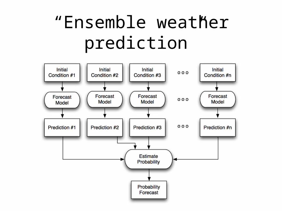
“Ensemble weather prediction”
Outline
• (1) Verification methods for evaluating ensemble (and probabilistic) forecasts
• (2) Numerical issues and principles. What more is there more to running an ensemble than slapping various forecasts together?
• (3) Examples of how ensembles can and will be used operationally to improve decisions.
4
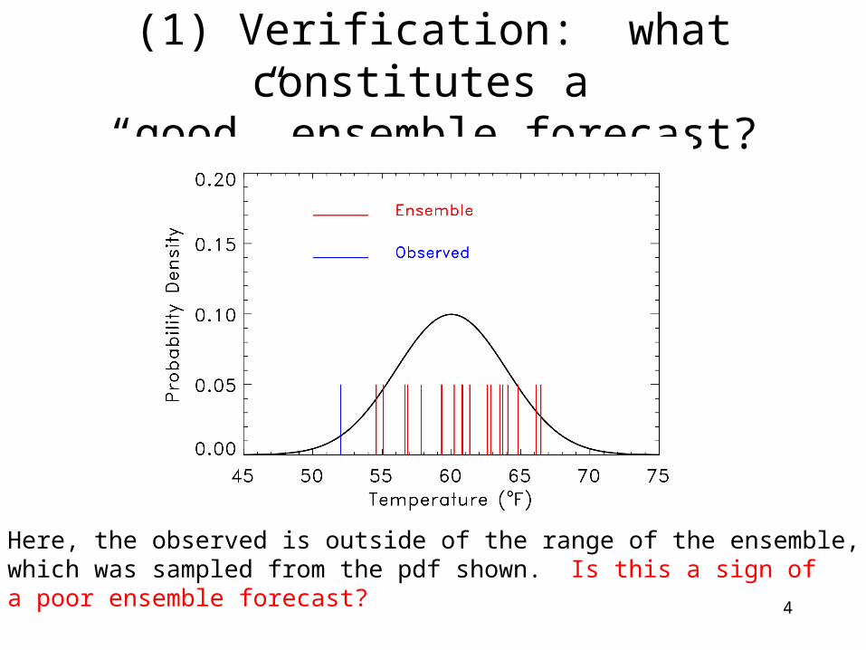
(1) Verification: what constitutes a “good” ensemble forecast?
Here, the observed is outside of the range of the ensemble,which was sampled from the pdf shown. Is this a sign ofa poor ensemble forecast?
5
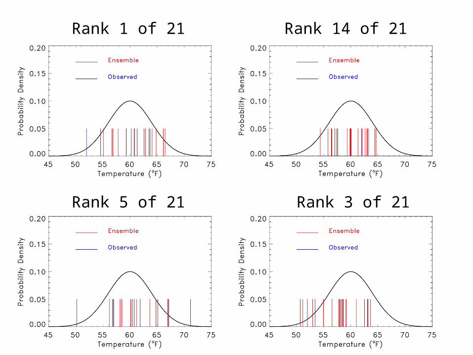
Rank 1 of 21 Rank 14 of 21
Rank 5 of 21 Rank 3 of 21

6
One way of evaluating ensembles: “rank histograms” or “Talagrand diagrams”
Happens whenobserved is indistinguishablefrom any other member of theensemble. Ensemble
is “reliable”
Happens when observed too commonly islower than the ensemble members.
Happens whenthere are eithersome low and somehigh biases, or whenthe ensemble doesn’tspread out enough.
We need lots of samples from many situations to evaluate the characteristics of the ensemble.
ref: Hamill, MWR, March 2001
7
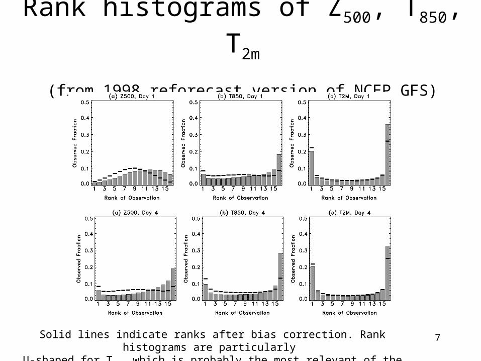
Rank histograms of Z500, T850, T2m
(from 1998 reforecast version of NCEP GFS)
Solid lines indicate ranks after bias correction. Rank histograms are particularly U-shaped for T2M, which is probably the most relevant of the three plotted here.
8
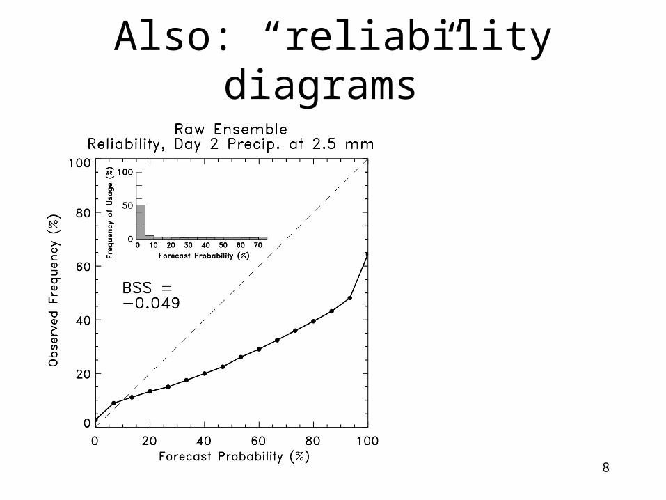
Also: “reliability diagrams”
9
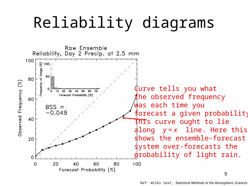
Reliability diagrams
Curve tells you whatthe observed frequencywas each time youforecast a given probability.This curve ought to liealong y = x line. Here thisshows the ensemble-forecastsystem over-forecasts theprobability of light rain.
Ref: Wilks text, Statistical Methods in the Atmospheric Sciences
10
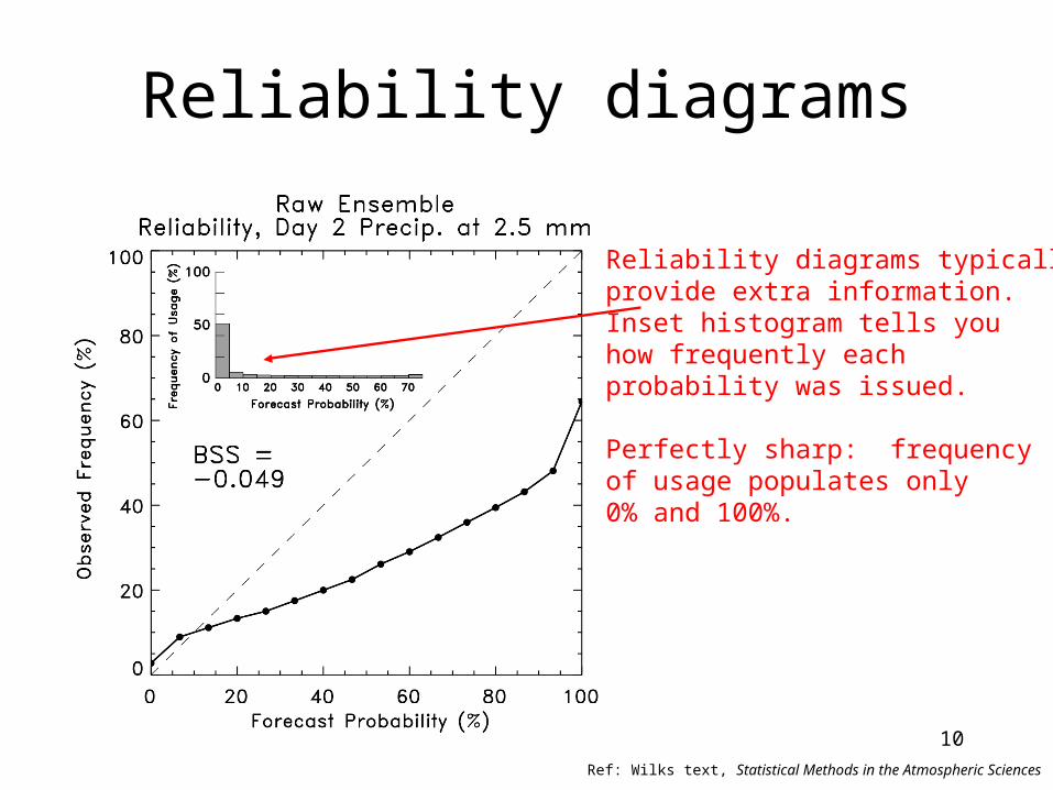
Reliability diagrams
Reliability diagrams typicallyprovide extra information.Inset histogram tells you how frequently each probability was issued.
Perfectly sharp: frequency of usage populates only0% and 100%.
Ref: Wilks text, Statistical Methods in the Atmospheric Sciences

11
Reliability diagramsBSS = Brier Skill Score
BSS =BS(CLimo)−BS(Forecast)BS(CLimo)−BS(Perfect)
BS(•) measures theBrier Score, which youcan think of as the squared error of a probabilistic forecast.
Perfect: BSS = 1.0Climatology: BSS = 0.0
A perfect BSS occurs onlywhen you forecast probabilitiesof 0 and 1 (and are perfectlyreliable).
Ref: Wilks text, Statistical Methods in the Atmospheric Sciences

12
Brier score• Define an event, e.g., obs. precip > 2.5 mm.• Let be the forecast probability for the ith
forecast case.• Let be the observed probability (1 or 0).
Then
Pif
Oi
BS(forecast) =1
ncasesPi
f −Oi( )i=1
ncases∑2
(So the Brier score is the averaged squared error ofthe probabilistic forecast)
13
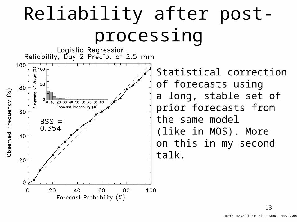
Reliability after post-processing
Statistical correctionof forecasts using a long, stable set ofprior forecasts fromthe same model (like in MOS). Moreon this in my secondtalk.
Ref: Hamill et al., MWR, Nov 2006
14
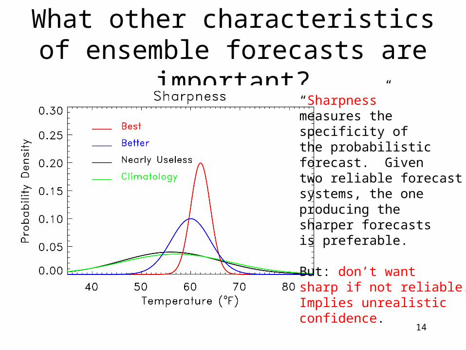
What other characteristics of ensemble forecasts are important?
“Sharpness”measures thespecificity ofthe probabilisticforecast. Given two reliable forecastsystems, the one producing the sharper forecastsis preferable.
But: don’t wantsharp if not reliable.Implies unrealistic confidence.

15
“Spread-skill” relationships are important, too.
ensemble-meanerror from a sampleof this pdf on avg.should be low.
ensemble-meanerror should bemoderate on avg.
ensemble-meanerror should belarge on avg.
Small-spread ensemble forecasts should have less ensemble-mean error than large-spread forecasts.

More verification topics (see backup slides)
• Continuous ranked probability score (CRPS).• Relative Operating Characteristic• Potential Economic Value• Issues with calculating skill - exaggerated skill
when combining samples from regions with different climatologies
• Evaluating multi-dimensional characteristics of ensembles.
(2) Ensemble prediction:numerical issues & principles
• Initial conditions should be consistent with analysis errors and should grow rapidly.
• Given forecast model is imperfect, ensemble should include methods for uncertainty of the models themselves.
• For regional ensembles, careful consideration of domain size & treatment of lateral boundary conditions essential.
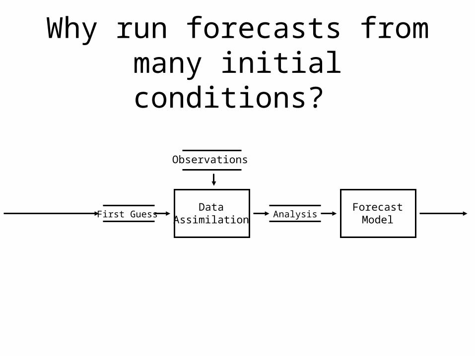
Why run forecasts from many initial conditions?
DataAssimilation
First Guess
Observations
AnalysisForecast
Model

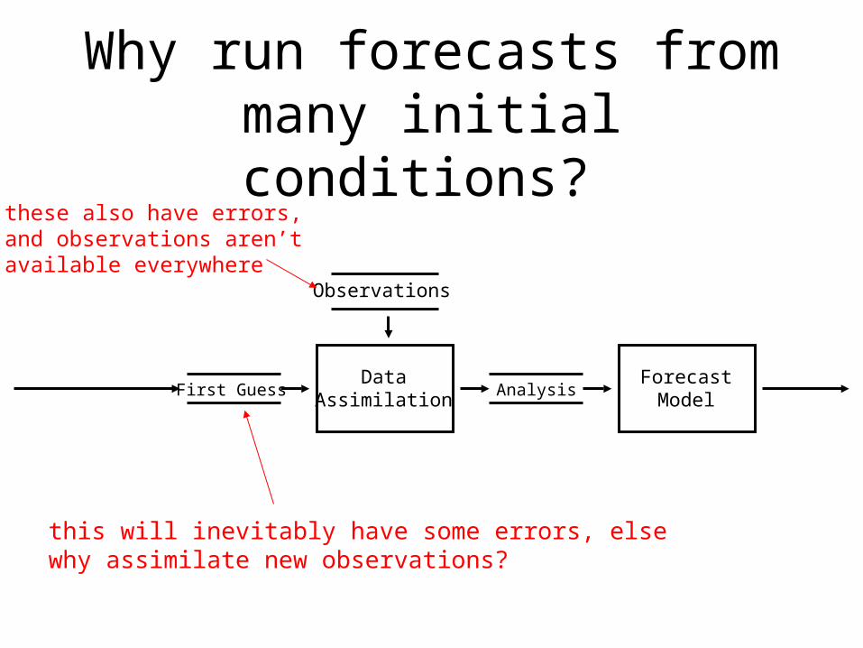
Why run forecasts from many initial conditions?
DataAssimilation
First Guess
Observations
Analysis
these also have errors,and observations aren’t available everywhere
ForecastModel
Why run forecasts from many initial conditions?
DataAssimilation
First Guess
Observations
Analysis
this will inevitably have some errors, elsewhy assimilate new observations?
ForecastModel
these also have errors,and observations aren’t available everywhere

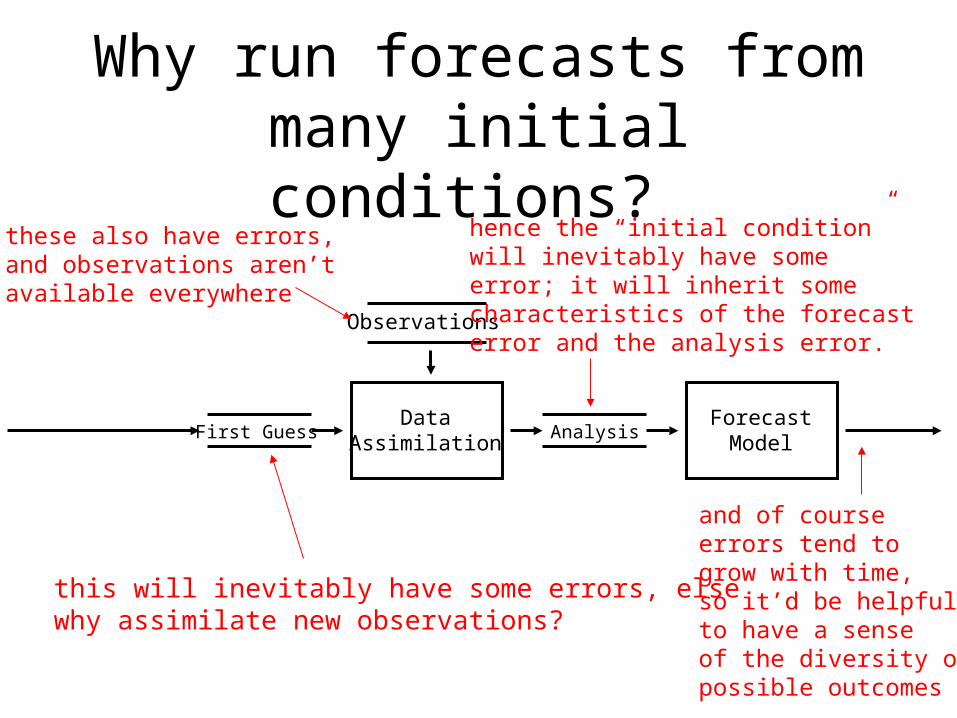
Why run forecasts from many initial conditions?
DataAssimilation
First Guess
Observations
Analysis
this will inevitably have some errors, elsewhy assimilate new observations?
these also have errors,and observations aren’t available everywhere
ForecastModel
hence the “initial condition”will inevitably have some error; it will inherit somecharacteristics of the forecasterror and the analysis error.
and of courseerrors tend togrow with time, so it’d be helpfulto have a senseof the diversity ofpossible outcomes
Preferred characteristics of ensemble initial conditions
• Differences between initial conditions should be larger:– in regions with few observations – in storm tracks, where past forecast differences
have grown quickly– where model dynamics are not accurate.
• Should perturb aspects of model state where– state is not estimated accurately.– model forecasts are sensitive to small changes in
state.
2424
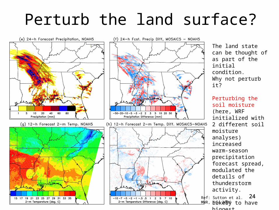
Perturb the land surface?
The land state can be thought of as part of the initial condition.Why not perturb it?
Perturbing the soil moisture (here, WRF initialized with 2 different soil moistureanalyses) increased warm-season precipitation forecast spread, modulated thedetails of thunderstormactivity.
Likely to have biggestimpact in warm season,when insolation is large. Though In winter, perturb snow cover/depth?
Ref: Sutton et al.MWR, Nov 2006
25
Model errors at mesoscale: higher resolution is important, but it’s
more than just that.
• Land-surface parameterization• Boundary-layer parameterization• Convective parameterization• Microphysical parameterization• etc.
26
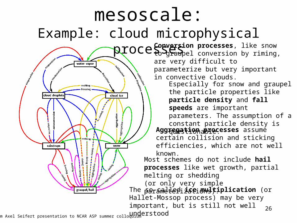
Model error at mesoscale:Example: cloud microphysical processes
Conversion processes, like snow to graupel conversion by riming, are very difficult to parameterize but very important in convective clouds.
Especially for snow and graupel the particle properties like particle density and fall speeds are important parameters. The assumption of a constant particle density is questionable.
Aggregation processes assume certain collision and sticking efficiencies, which are not well known.
Most schemes do not include hail processes like wet growth, partial melting or shedding (or only very simple parameterizations).
The so-called ice multiplication (or Hallet-Mossop process) may be very important, but is still not well understood
from Axel Seifert presentation to NCAR ASP summer colloquium
27
Model error at mesoscale:Summary of microphysical issues
in convection-resolving NWP
• Many fundamental problems in cloud microphysics are still unsolved.
• The lack of in-situ observations makes any progress very slow and difficult.
• Most of the current parameterization have been designed, operationally applied and tested for stratiform precipitation only.
• Most of the empirical relations used in the parameterizations are based on surface observation or measurements in stratiform cloud (or storm anvils, stratiform regions).
• Many basic parameterization assumptions, like N0=const., are at least questionable in convective clouds.
• Many processes which are currently neglected, or not well represented, may become important in deep convection (shedding, collisional breakup, ...).
• One-moment schemes might be insufficient to describe the variability of the size distributions in convective clouds.
• Two-moment schemes haven‘t been used long enough to make any conclusions.
• Spectral methods are overwhelmingly complicated and computationally expensive. Nevertheless, they suffer from our lack of understanding of the fundamental processes.
from Axel Seifert presentation to NCAR ASP summer colloquium
28
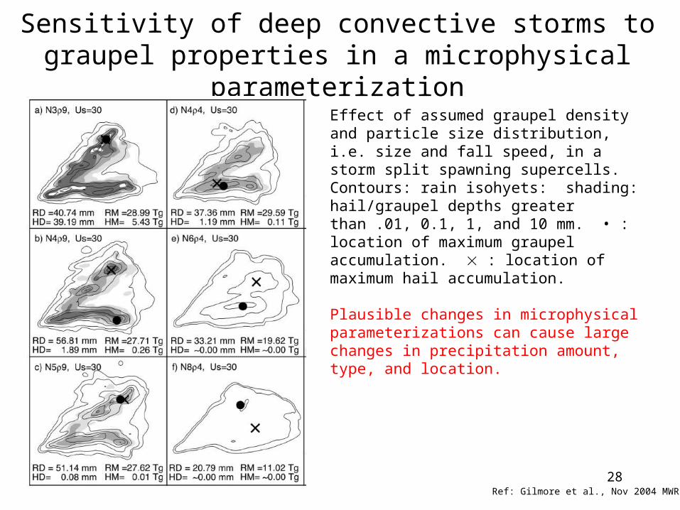
Sensitivity of deep convective storms to graupel properties in a microphysical parameterization
Ref: Gilmore et al., Nov 2004 MWR
Effect of assumed graupel density and particle size distribution, i.e. size and fall speed, in a storm split spawning supercells. Contours: rain isohyets: shading: hail/graupel depths greater than .01, 0.1, 1, and 10 mm. • : location of maximum graupel accumulation. : location of maximum hail accumulation.
Plausible changes in microphysical parameterizations can cause large changes in precipitation amount, type, and location.

What is commonly done to deal with model error
• Increase resolution• Use multiple forecast models.• Use multiple parameterizations.• Use multiple constants in parameterizations.• Introduce stochastic elements into
deterministic forecast model.
There isn’t a clean, unifying theory guiding us on model error.

3030
Lateral boundary conditions(now universally accepted that perturbed LBCs necessary
in limited-area ensembles)
0-h
12-h
24-h
36-h
Perturb both IC & LBC
Perturb LBC only
Example:
SREF Z500 spreadfor a 19 May 98case of 5-member,32-km Eta modelensemble.
(only small impacton precipitation field)
Ref: Du and Tracton,1999, WMO reportfor WGNE.
Perturb IC only

3131
Lateral boundary condition issues for LAMs (and LAEFs)
• With 1-way LBCs, small scales in domain cannot interact with scales larger than some limit defined by domain size.
• LBCs generally provided by coarser-resolution forecast models, and this “sweeps” in low-resolution information, sweeps out developing high-resolution information.
• Physical process parameterizations for model driving LBCs may be different than for interior. Can cause spurious gradients
• LBC info may introduce erroneous information for other reasons, e.g., model numerics.
• LBC initialization can produce transient gravity-inertia modes.
Ref: Warner et al. review article, BAMS, November 1997

3232
Influence of domain size
T-126 global model drivinglateral boundary conditionsfor nests with 80-km and 40-km grid spacingof limited-area model.
from Warner et al. Nov 1997 BAMS, and Treadon and Peterson (1993), Preprints, 13thConf. on Weather Analysis and Forecasting
3333
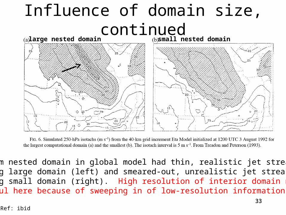
Influence of domain size, continued
40-km nested domain in global model had thin, realistic jet streak using large domain (left) and smeared-out, unrealistic jet streak using small domain (right). High resolution of interior domain notuseful here because of sweeping in of low-resolution information.
large nested domain small nested domain
Ref: ibid
(3) Use of ensembles for improving decisions
35
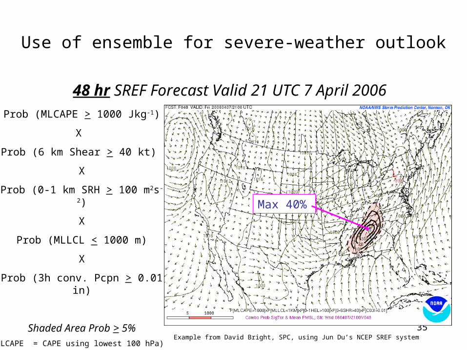
Use of ensemble for severe-weather outlook
48 hr SREF Forecast Valid 21 UTC 7 April 2006
Prob (MLCAPE > 1000 Jkg-1)
X
Prob (6 km Shear > 40 kt)
X
Prob (0-1 km SRH > 100 m2s-2)
X
Prob (MLLCL < 1000 m)
X
Prob (3h conv. Pcpn > 0.01 in)
Shaded Area Prob > 5%
Max 40%
(MLCAPE = CAPE using lowest 100 hPa)Example from David Bright, SPC, using Jun Du’s NCEP SREF system
36
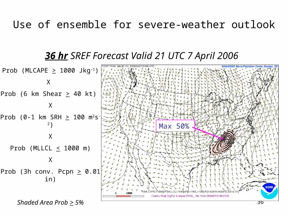
Use of ensemble for severe-weather outlook
36 hr SREF Forecast Valid 21 UTC 7 April 2006
Prob (MLCAPE > 1000 Jkg-1)
X
Prob (6 km Shear > 40 kt)
X
Prob (0-1 km SRH > 100 m2s-2)
X
Prob (MLLCL < 1000 m)
X
Prob (3h conv. Pcpn > 0.01 in)
Shaded Area Prob > 5%
Max 50%
37
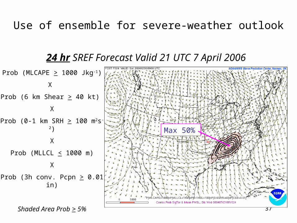
24 hr SREF Forecast Valid 21 UTC 7 April 2006
Prob (MLCAPE > 1000 Jkg-1)
X
Prob (6 km Shear > 40 kt)
X
Prob (0-1 km SRH > 100 m2s-2)
X
Prob (MLLCL < 1000 m)
X
Prob (3h conv. Pcpn > 0.01 in)
Shaded Area Prob > 5%
Max 50%
Use of ensemble for severe-weather outlook
38
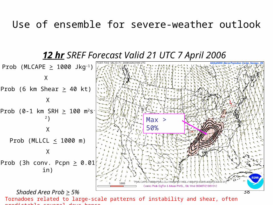
12 hr SREF Forecast Valid 21 UTC 7 April 2006Prob (MLCAPE > 1000 Jkg-1)
X
Prob (6 km Shear > 40 kt)
X
Prob (0-1 km SRH > 100 m2s-2)
X
Prob (MLLCL < 1000 m)
X
Prob (3h conv. Pcpn > 0.01 in)
Shaded Area Prob > 5%
Max > 50%
Use of ensemble for severe-weather outlook
Tornadoes related to large-scale patterns of instability and shear, often predictable several days hence.
39
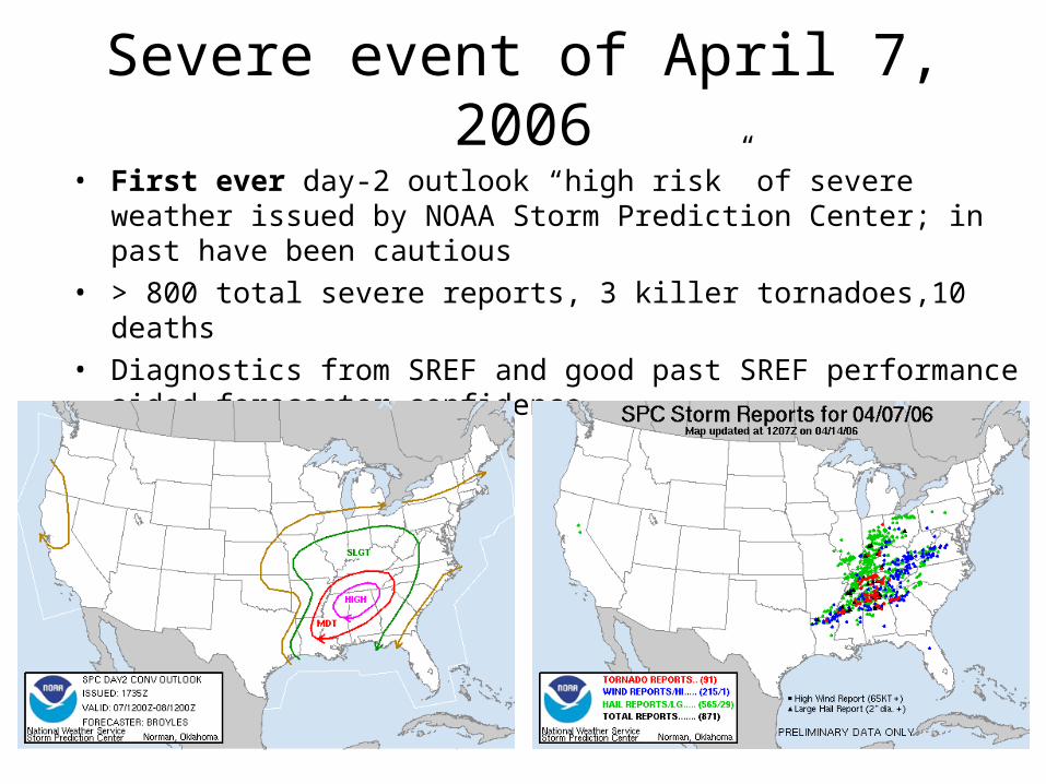
Severe event of April 7, 2006• First ever day-2 outlook “high risk” of severe weather issued by
NOAA Storm Prediction Center; in past have been cautious• > 800 total severe reports, 3 killer tornadoes,10 deaths • Diagnostics from SREF and good past SREF performance aided
forecaster confidence
40
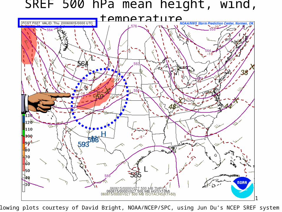
Example of predicting extreme event from ensemble: USfire-weather forecasting
• Ingredients from large-scale conditions:– High wind speeds– Hot temperatures– Low relative humidity near surface– Little rainfall
41
SREF 500 hPa mean height, wind, temperature
Following plots courtesy of David Bright, NOAA/NCEP/SPC, using Jun Du’s NCEP SREF system
42
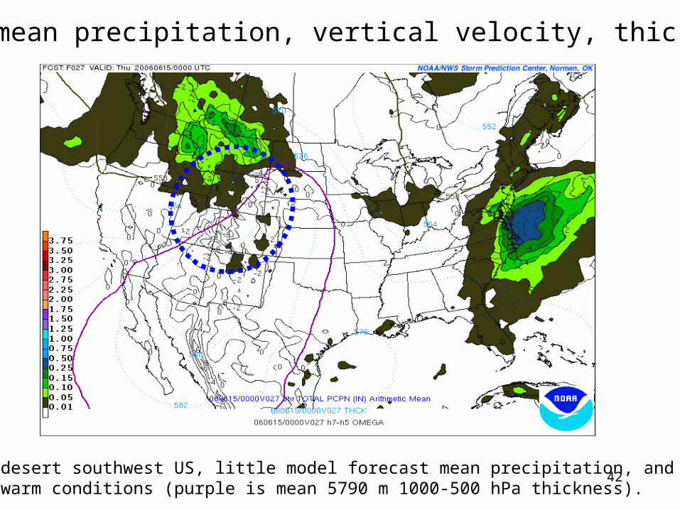
SREF mean precipitation, vertical velocity, thickness
Over desert southwest US, little model forecast mean precipitation, and very warm conditions (purple is mean 5790 m 1000-500 hPa thickness).

43
SREF Pr[P12I > .01”] and Mean P12I = .01” (dash)
Some members forecasting precipitation over Colorado,New Mexico, but southern Utah and Arizona forecast dry.
44
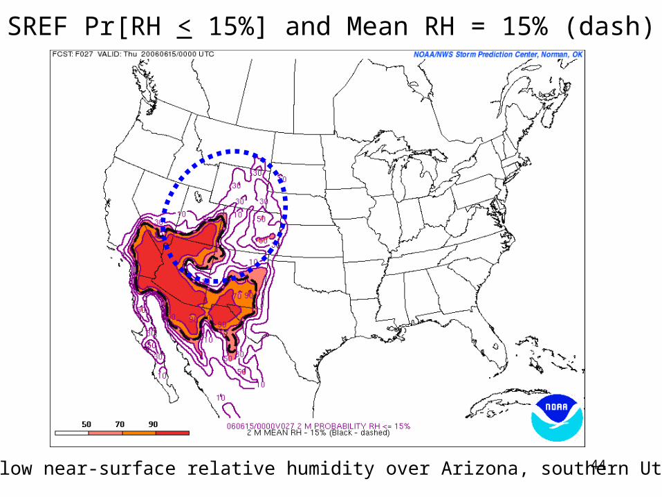
SREF Pr[RH < 15%] and Mean RH = 15% (dash)
very low near-surface relative humidity over Arizona, southern Utah
45
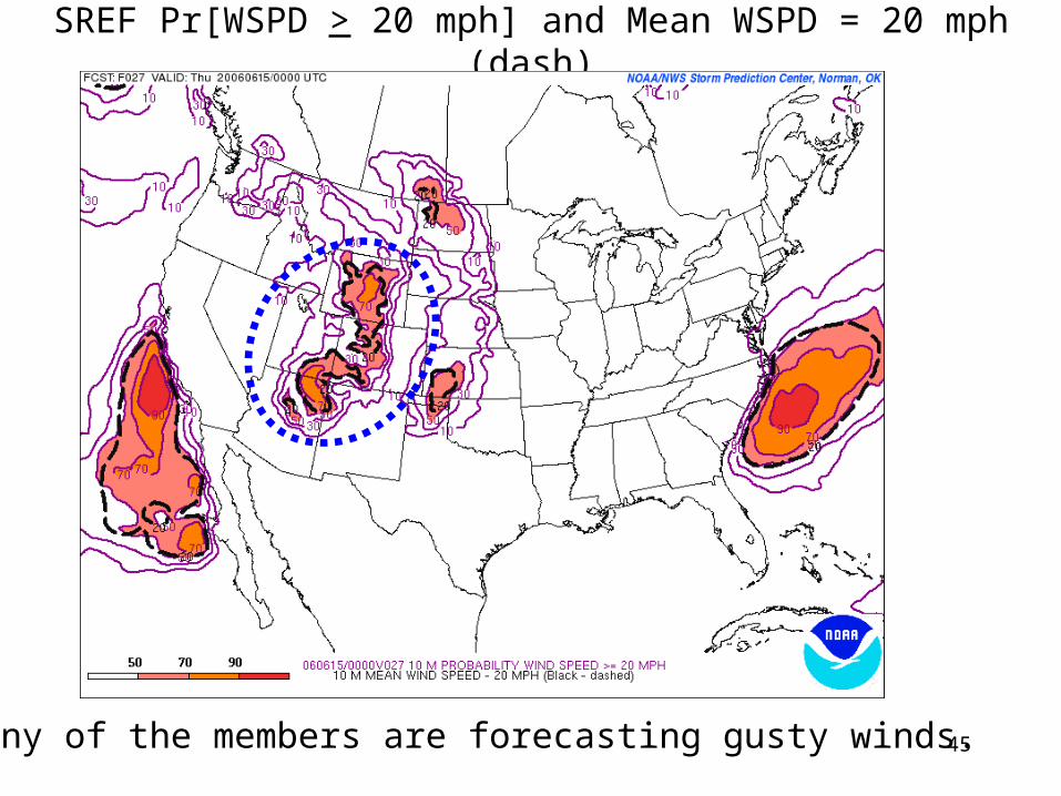
SREF Pr[WSPD > 20 mph] and Mean WSPD = 20 mph (dash)
Many of the members are forecasting gusty winds.
46
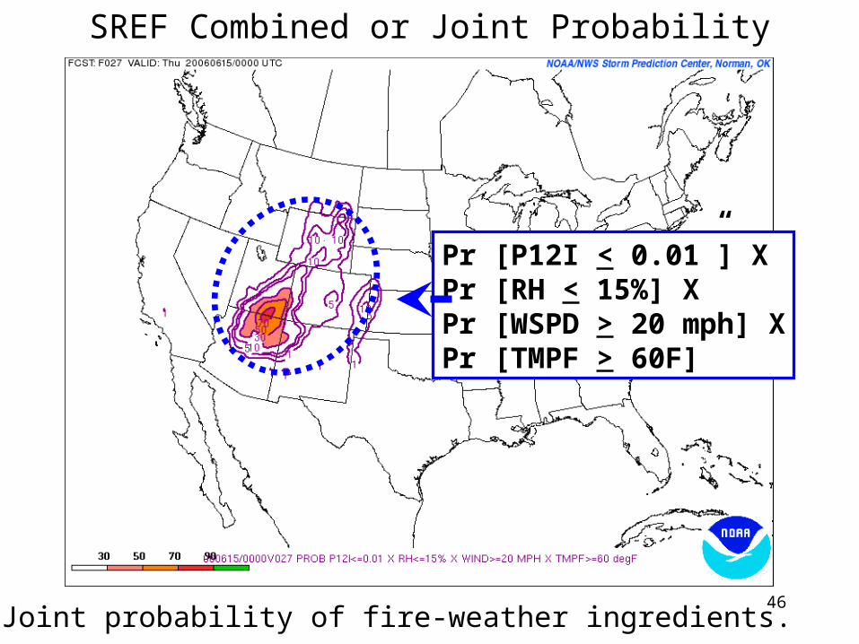
SREF Combined or Joint Probability
Pr [P12I < 0.01”] XPr [RH < 15%] XPr [WSPD > 20 mph] XPr [TMPF > 60F]
Joint probability of fire-weather ingredients.

47
NOAA SPC Operational Outlook(Uncertainty communicated in accompanying text)
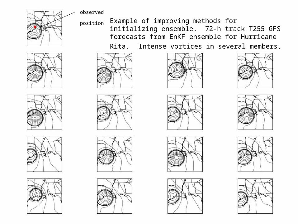
Example of improving methods for initializing ensemble. 72-h track T255 GFS forecasts from EnKF ensemble for
Hurricane Rita. Intense vortices in several members.
observed
position

NHC official track forecast(note: official track far south of actual track,
south of EnKF ensemble track forecast)
Take-home messages as we move to ensemble prediction
• A new probabilistic forecast paradigm requires verifying in new ways, measuring “reliability” and “sharpness.”
• Ensemble prediction requires more than slapping some control forecasts together; there are numerical principles to be followed.
• Better decisions, or advanced lead time for decisions, are possible by utilizing ensembles.
51
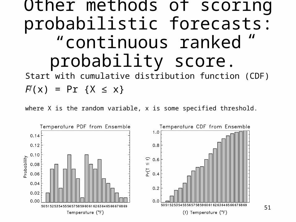
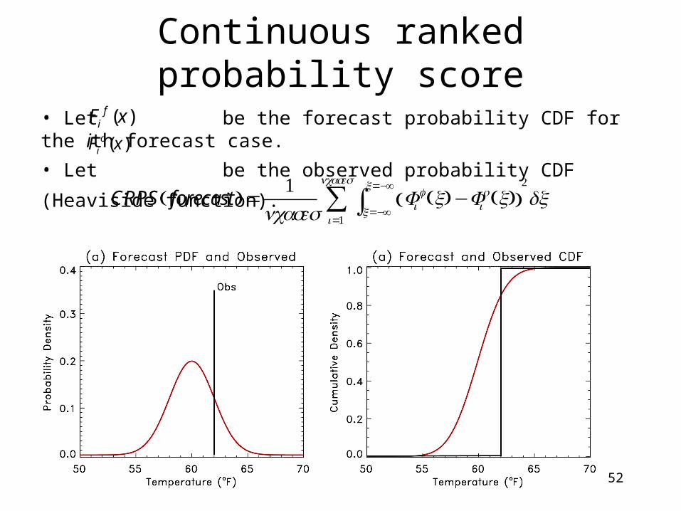
Other methods of scoring probabilistic forecasts: “continuous
ranked probability score.”Start with cumulative distribution function (CDF)
Ff(x) = Pr {X ≤ x}
where X is the random variable, x is some specified threshold.
52
Continuous ranked probability score
• Let be the forecast probability CDF for the ith forecast case.
• Let be the observed probability CDF (Heaviside function).
Fif (x)
Fio(x)
CRPS forecast( ) =1
ncasesFi
f (x)−Fio(x)( )
x=−∞
x=−∞
∫2
dxi=1
ncases
∑
53
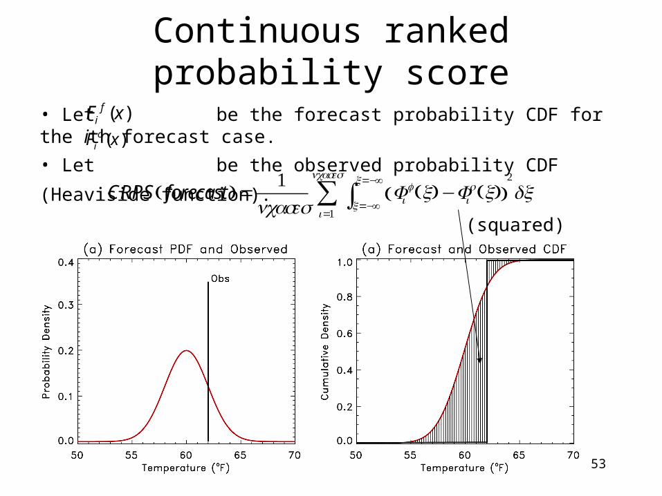
Continuous ranked probability score
• Let be the forecast probability CDF for the ith forecast case.
• Let be the observed probability CDF (Heaviside function).
Fif (x)
Fio(x)
CRPS forecast( ) =1
ncasesFi
f (x)−Fio(x)( )
x=−∞
x=−∞
∫2
dxi=1
ncases
∑(squared)

54
Continuous ranked probability skill score (CRPSS)
CRPSS =CRPS( forecast)−CRPS(climo)CRPS(perfect)−CRPS(climo)
Like the Brier score, it’s common to convert this toa skill score by normalizing by the skill of climatology,or some other reference.
Ref: Wilks 2006 text
55
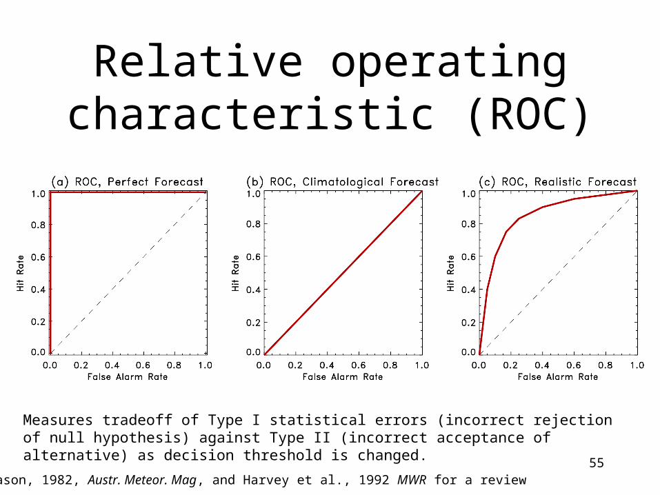
Relative operating characteristic (ROC)
see Mason, 1982, Austr. Meteor. Mag, and Harvey et al., 1992 MWR for a review
Measures tradeoff of Type I statistical errors (incorrect rejection of null hypothesis) against Type II (incorrect acceptance of alternative) as decision threshold is changed.
56
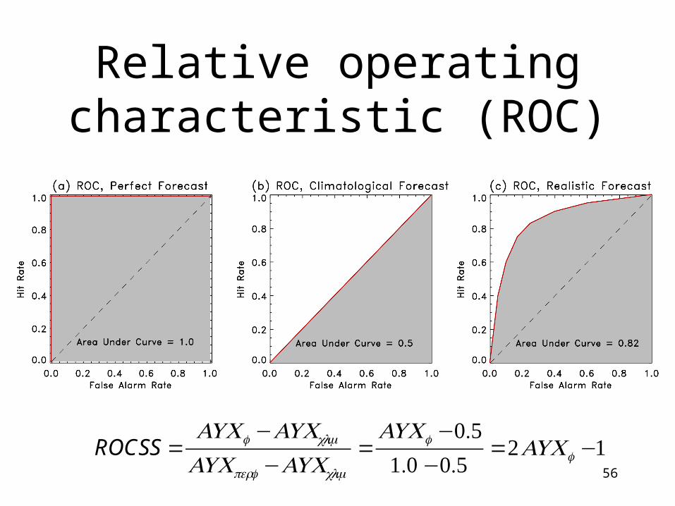
Relative operating characteristic (ROC)
ROCSS =AUC f −AUCclim
AUCperf −AUCclim
=AUC f −0.51.0 −0.5
=2AUC f −1

57
Method of calculation of ROC:parts 1 and 2
Y N
Y 0 0
N 0 1
55 56 57 58 59 60 61 62 63 64 65 66
T
F FFFFF
Obs ≥ T?
Fcs
t ≥ T
?
(1) Build contingency tables for each sorted ensemble member
Obs
Y N
Y 0 0
N 0 1
Obs ≥ T?
Fcs
t ≥ T
?
Y N
Y 0 0
N 0 1
Obs ≥ T?
Fcs
t ≥ T
?
Y N
Y 0 1
N 0 0
Obs ≥ T?F
cst ≥
T?
Y N
Y 0 1
N 0 0
Obs ≥ T?
Fcs
t ≥ T
?
Y N
Y 0 1
N 0 0
Obs ≥ T?
Fcs
t ≥ T
?
(2) Repeat the process for other locations, dates, buildingup contingency tables for sorted members.
58
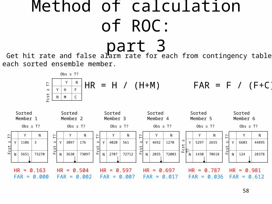
Method of calculation of ROC:part 3
Y N
Y 4020 561
N 2707 72712
Obs ≥ T?
Fcs
t ≥ T
?
(3) Get hit rate and false alarm rate for each from contingency table for each sorted ensemble member.
Obs ≥ T?
Fcs
t ≥ T
?
Obs ≥ T?
Fcs
t ≥ T
?
Obs ≥ T?
Fcs
t ≥ T
?
Obs ≥ T?
Fcs
t ≥ T
?
Obs ≥ T?
Fcs
t ≥ T
?
Y N
Y H F
N M C
Obs ≥ T?
Fcs
t ≥ T
? HR = H / (H+M) FAR = F / (F+C)
Sorted Member 1
Sorted Member 2
Sorted Member 3
Sorted Member 4
Sorted Member 5
Sorted Member 6
Y N
Y 1106 3
N 5651 73270
Y N
Y 4692 1270
N 2035 72003
Y N
Y 3097 176
N 3630 73097
Y N
Y 5297 2655
N 1430 70618
Y N
Y 6603 44895
N 124 28378
HR = 0.163FAR = 0.000
HR = 0.504FAR = 0.002
HR = 0.597FAR = 0.007
HR = 0.697FAR = 0.017
HR = 0.787FAR = 0.036
HR = 0.981FAR = 0.612
59
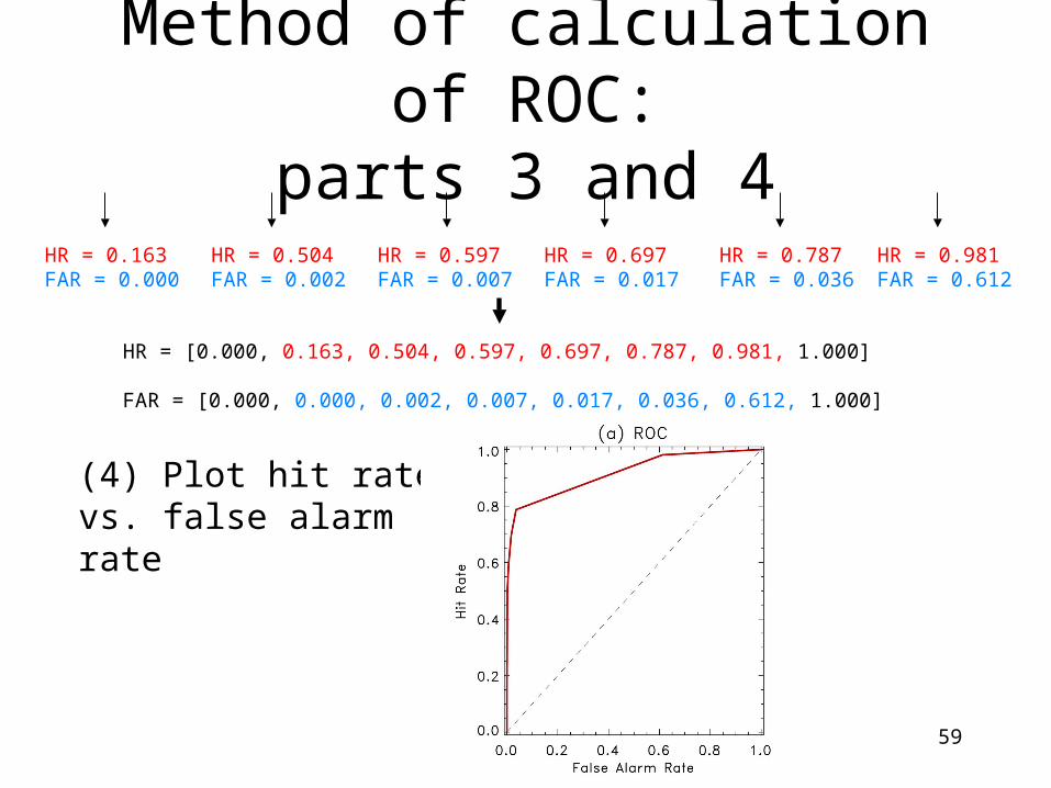
Method of calculation of ROC:parts 3 and 4
HR = 0.163FAR = 0.000
HR = 0.504FAR = 0.002
HR = 0.597FAR = 0.007
HR = 0.697FAR = 0.017
HR = 0.787FAR = 0.036
HR = 0.981FAR = 0.612
HR = [0.000, 0.163, 0.504, 0.597, 0.697, 0.787, 0.981, 1.000]
FAR = [0.000, 0.000, 0.002, 0.007, 0.017, 0.036, 0.612, 1.000]
(4) Plot hit ratevs. false alarmrate
60
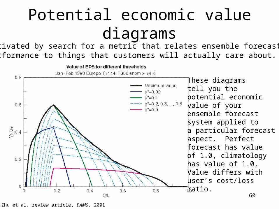
Potential economic value diagrams
These diagramstell you the potential economicvalue of yourensemble forecastsystem applied toa particular forecastaspect. Perfectforecast has valueof 1.0, climatologyhas value of 1.0.Value differs withuser’s cost/lossratio.
Motivated by search for a metric that relates ensemble forecastperformance to things that customers will actually care about.
from Zhu et al. review article, BAMS, 2001
61
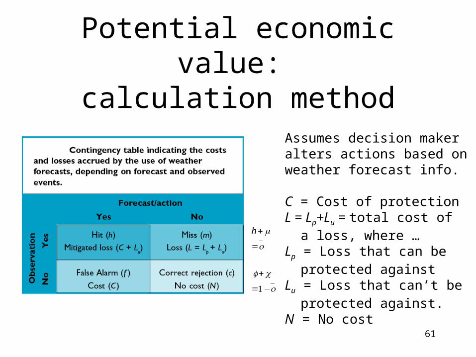
Potential economic value: calculation method
Assumes decision makeralters actions based on weather forecast info.
C = Cost of protectionL = Lp+Lu = total cost of a loss, where …Lp = Loss that can be protected againstLu = Loss that can’t be protected against.N = No cost
h +m
=o
f + c
=1−o

62
Potential economic value, continuedSuppose we have the contingencytable of forecast outcomes, [h, m, f, c].
Then we can calculate the expectedvalue of the expenses from a forecast,from climatology, from a perfect forecast.
E forecast = fC +h C + Lu( ) +m Lp + Lu( )
Eclimate =Min o Lp + Lu( ), C + oLu⎡⎣ ⎤⎦=oLu + Min oLp, C⎡⎣ ⎤⎦
Eperfect =o C + Lu( )
V =Eclimate −E forecast
Eclimate −Eperfect
=Min oLp, C⎡⎣ ⎤⎦− h+ f( )C −mLp
Min oLp, C⎡⎣ ⎤⎦−oC
Note thatvalue will varywith C, Lp, Lu;
Different userswith different protection costsmay experiencea different valuefrom the forecastsystem.
h +m
=o
f + c
=1−o
63
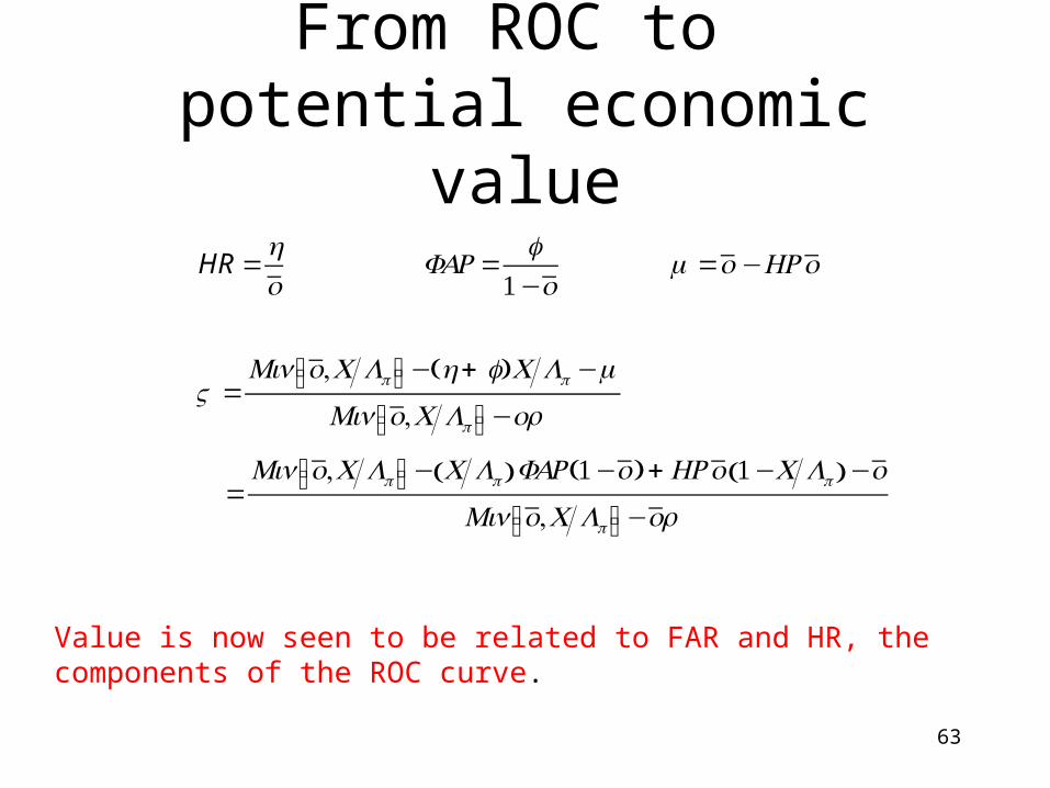
From ROC to potential economic value
HR =ho
FAR=f
1−om=o−HRo
V =Min o,C Lp⎡⎣ ⎤⎦− h+ f( )C Lp −m
Min o,C Lp⎡⎣ ⎤⎦−or
=Min o,C Lp⎡⎣ ⎤⎦− C Lp( )FAR 1−o( ) + HRo 1−C Lp( )−o
Min o,C Lp⎡⎣ ⎤⎦−or
Value is now seen to be related to FAR and HR, the components of the ROC curve.

64
The red curve isfrom the ROCdata for the member defining the 90th percentile of the ensemble distribution.Green curve is forthe 10th percentile.Overall economicvalue is the maximum(use whatever memberfor decision threshold that provides thebest economic value).
Economic value curve example
While admirable for framing verification in terms more relevant to the forecast user, the economic value calculations as presented here do not take into account other
factors such as risk-aversion, or more complex decisions other than protect/don’t.

65
Forecast skill often overestimated!- Suppose you have a sample of forecasts from two islands, and each island has different climatology.
- Weather forecasts impossible on both islands.
- Simulate “forecast” with an ensemble of draws from climatology
- Island 1: F ~ N(,1). Island 2: F ~ N(-,1)
- Calculate ROCSS, BSS, ETS in normal way. Expect no skill.
As climatology of the two islands begins to differ, then “skill” increases though samples drawn from climatology.
These scores falsely attribute differences in samples’ climatologies to skill of the forecast.
Samples must have the same climatological event frequency to avoid this.
reference: Hamill and Juras, QJRMS, Oct 2006
66
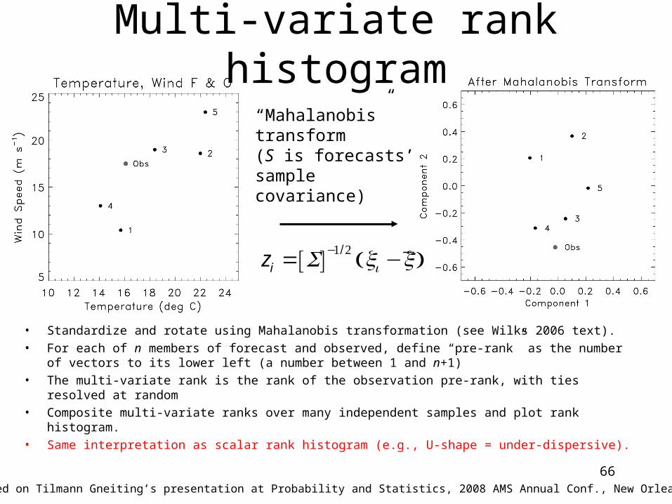
Multi-variate rank histogram
• Standardize and rotate using Mahalanobis transformation (see Wilks 2006 text).
• For each of n members of forecast and observed, define “pre-rank” as the number of vectors to its lower left (a number between 1 and n+1)
• The multi-variate rank is the rank of the observation pre-rank, with ties resolved at random
• Composite multi-variate ranks over many independent samples and plot rank histogram.
• Same interpretation as scalar rank histogram (e.g., U-shape = under-dispersive).
based on Tilmann Gneiting’s presentation at Probability and Statistics, 2008 AMS Annual Conf., New Orleans .
zi = S[ ]−1/2 xi −x( )
“Mahalanobis”transform(S is forecasts’samplecovariance)
67
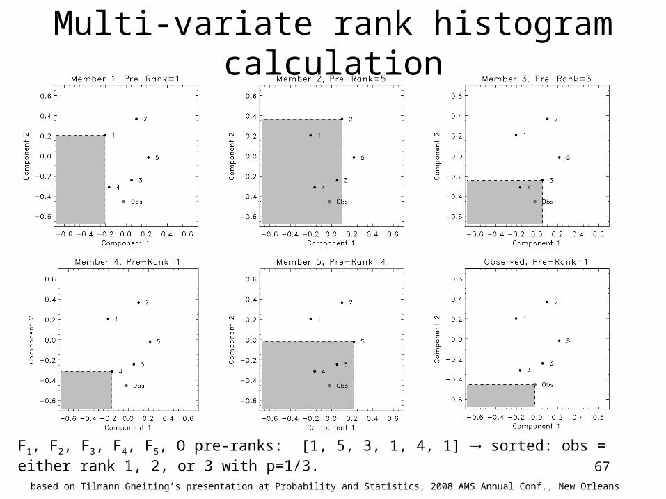
Multi-variate rank histogram calculation
based on Tilmann Gneiting’s presentation at Probability and Statistics, 2008 AMS Annual Conf., New Orleans
F1, F2, F3, F4, F5, O pre-ranks: [1, 5, 3, 1, 4, 1] sorted: obs = either rank 1, 2, or 3 with p=1/3.
68
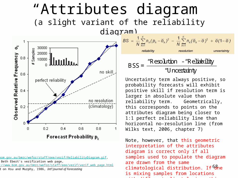
“Attributes diagram”(a slight variant of the reliability diagram)
www.bom.gov.au/bmrc/wefor/staff/eee/verif/ReliabilityDiagram.gif,from Beth Ebert’s verification web page,http://www.bom.gov.au/bmrc/wefor/staff/eee/verif/verif_web_page.htmlbased on Hsu and Murphy, 1986, Int’l Journal of Forecasting
BSS = “Resolution” - “Reliability”
“Uncertainty”Uncertainty term always positive, so probability forecasts will exhibit positive skill if resolution term is larger in absolute value than reliability term. Geometrically, this corresponds to points on the attributes diagram being closer to 1:1 perfect reliability line than horizontal no-resolution line (from Wilks text, 2006, chapter 7)
Note, however, that this geometric interpretation of the attributes diagram is correct only if all samples used to populate the diagram are drawn from the same climatological distribution. If one is mixing samples from locations with different climatologies, this interpretation is no longer correct! (for more on what underlies this issue, see Hamill and Juras, Oct 2006 QJRMS)
69
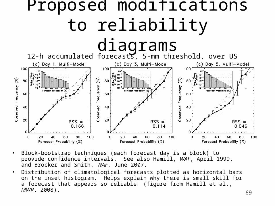
Proposed modifications to reliability diagrams
• Block-bootstrap techniques (each forecast day is a block) to provide confidence intervals. See also Hamill, WAF, April 1999, and Bröcker and Smith, WAF, June 2007.
• Distribution of climatological forecasts plotted as horizontal bars on the inset histogram. Helps explain why there is small skill for a forecast that appears so reliable (figure from Hamill et al., MWR, 2008).
12-h accumulated forecasts, 5-mm threshold, over US