enterprise scale topological data analysis using spark
TRANSCRIPT
ENTERPRISE-SCALE TOPOLOGICAL DATA ANALYSIS USING SPARK
Anshuman Mishra, Lawrence Spracklen Alpine Data
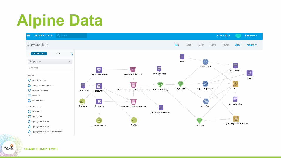
Alpine Data
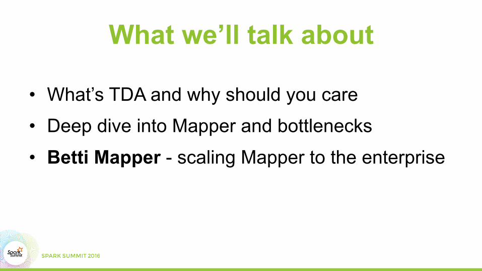
What we’ll talk about
• What’s TDA and why should you care
• Deep dive into Mapper and bottlenecks
• Betti Mapper - scaling Mapper to the enterprise

Can anyone recognize this?
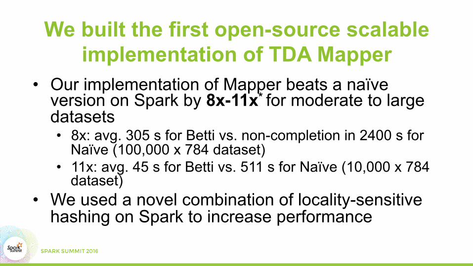
We built the first open-source scalable implementation of TDA Mapper
• Our implementation of Mapper beats a naïve version on Spark by 8x-11x* for moderate to large datasets • 8x: avg. 305 s for Betti vs. non-completion in 2400 s for
Naïve (100,000 x 784 dataset)
• 11x: avg. 45 s for Betti vs. 511 s for Naïve (10,000 x 784 dataset)
• We used a novel combination of locality-sensitive hashing on Spark to increase performance
TDA AND MAPPER: WHY SHOULD WE CARE?

Conventional ML carries the “curse of dimensionality”
• As d à∞, all data points are packed away into corners of a corresponding d-dimensional hypercube, with little to separate them
• Instance learners start to choke
• Detecting anomalies becomes tougher
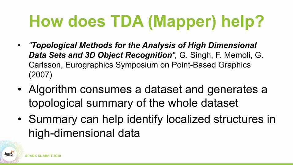
How does TDA (Mapper) help? • “Topological Methods for the Analysis of High Dimensional
Data Sets and 3D Object Recognition”, G. Singh, F. Memoli, G. Carlsson, Eurographics Symposium on Point-Based Graphics (2007)
• Algorithm consumes a dataset and generates a topological summary of the whole dataset
• Summary can help identify localized structures in high-dimensional data
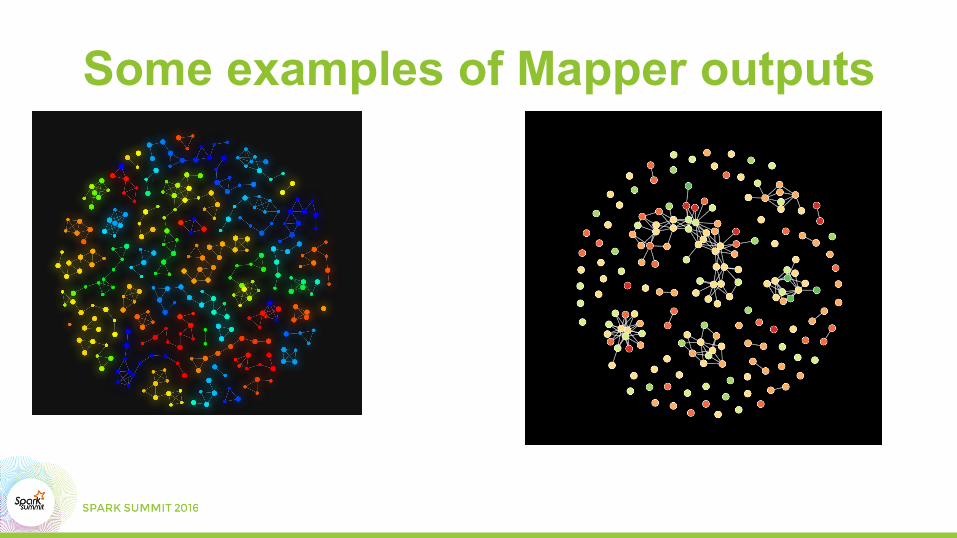
Some examples of Mapper outputs

DEEP DIVE INTO MAPPER

Mapper: The 30,000 ft. view
M x M distance matrix
M x N
M x 1
M x 1
. . .
. . .
.
. .
. . . . …
M x M distance matrix
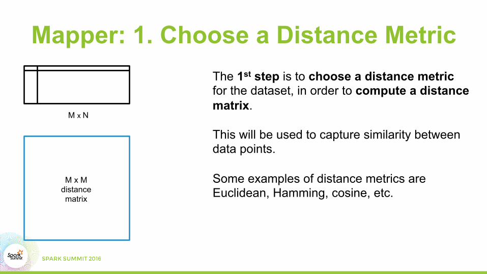
Mapper: 1. Choose a Distance Metric
M x N
The 1st step is to choose a distance metric for the dataset, in order to compute a distance matrix. This will be used to capture similarity between data points. Some examples of distance metrics are Euclidean, Hamming, cosine, etc.
M x M distance matrix
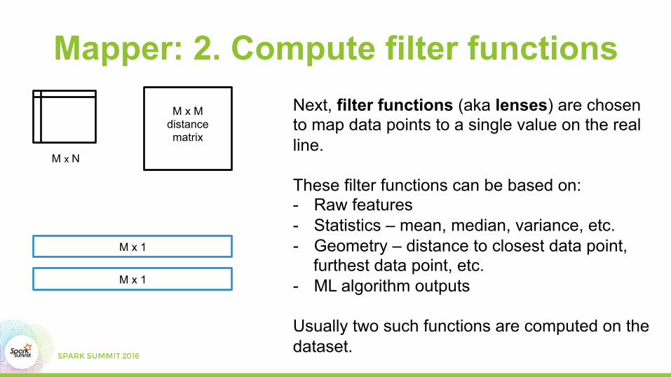
Mapper: 2. Compute filter functions
M x N
Next, filter functions (aka lenses) are chosen to map data points to a single value on the real line. These filter functions can be based on: - Raw features - Statistics – mean, median, variance, etc. - Geometry – distance to closest data point,
furthest data point, etc. - ML algorithm outputs
Usually two such functions are computed on the dataset.
M x 1
M x 1

M x M distance matrix
Mapper: 3. Apply cover & overlap
M x N
M x 1
M x 1
…
Next, the ranges of each filter application are “chopped up” into overlapping segments or intervals using two parameters: cover and overlap - Cover (aka resolution) controls how many
intervals each filter range will be chopped into, e.g. 40,100
- Overlap controls the degree of overlap between intervals (e.g. 20%)
Cover
Overlap
M x M distance matrix
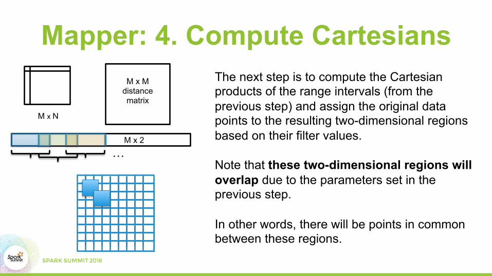
Mapper: 4. Compute Cartesians
M x N
The next step is to compute the Cartesian products of the range intervals (from the previous step) and assign the original data points to the resulting two-dimensional regions based on their filter values. Note that these two-dimensional regions will overlap due to the parameters set in the previous step. In other words, there will be points in common between these regions.
M x 2
…

M x M distance matrix
Mapper: 5. Perform clustering M x N
The penultimate stage in the Mapper algorithm is to perform clustering in the original high-dimensional space for each (overlapping) region. Each cluster will be represented by a node; since regions overlap, some clusters will have points in common. Their corresponding nodes will be connected via an unweighted edge. The kind of clustering performed is immaterial. Our implementation uses DBSCAN.
M x 2
…
. . .
. . .
. . .
. . . .
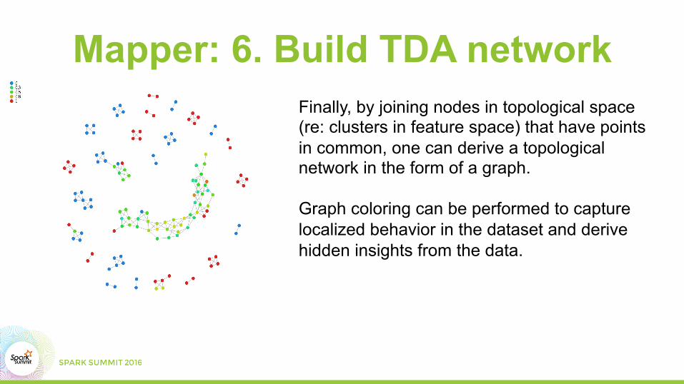
Mapper: 6. Build TDA network Finally, by joining nodes in topological space (re: clusters in feature space) that have points in common, one can derive a topological network in the form of a graph. Graph coloring can be performed to capture localized behavior in the dataset and derive hidden insights from the data.
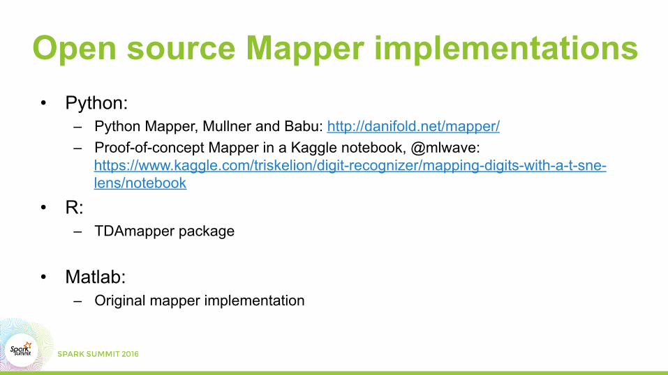
Open source Mapper implementations • Python:
– Python Mapper, Mullner and Babu: http://danifold.net/mapper/ – Proof-of-concept Mapper in a Kaggle notebook, @mlwave:
https://www.kaggle.com/triskelion/digit-recognizer/mapping-digits-with-a-t-sne-lens/notebook
• R: – TDAmapper package
• Matlab: – Original mapper implementation

Alpine TDA R
Python

Mapper: Computationally expensive!
M x M distance matrix
M x N
M x 1
M x 1
. . .
. . .
.
. .
. . . . …
O(N2) is prohibitive for large datasets
Single-node open source Mappers choke on large datasets (generously defined as > 10k data points with >100 columns)
Rolling our own Mapper.. • Our Mapper implementation
– Built on PySpark 1.6.1 – Called Betti Mapper – Named after Enrico Betti, a famous topologist
X ✔

Multiple ways to scale Mapper 1. Naïve Spark implementation
ü Write the Mapper algorithm using (Py)Spark RDDs – Distance matrix computation still performed over entire dataset on
driver node
2. Down-sampling / landmarking (+ Naïve Spark) ü Obtain manageable number of samples from dataset – Unreasonable to assume global distribution profiles are captured
by samples
3. LSH Prototyping!!!!?!

What came first?
• We use Mapper to detect structure in high-dimensional data using the concept of similarity.
• BUT we need to measure similarity so we can sample efficiently. • We could use stratified sampling, but then what about
• Unlabeled data? • Anomalies and outliers?
• LSH is a lower-cost first pass capturing similarity for cheap and helping to scale Mapper
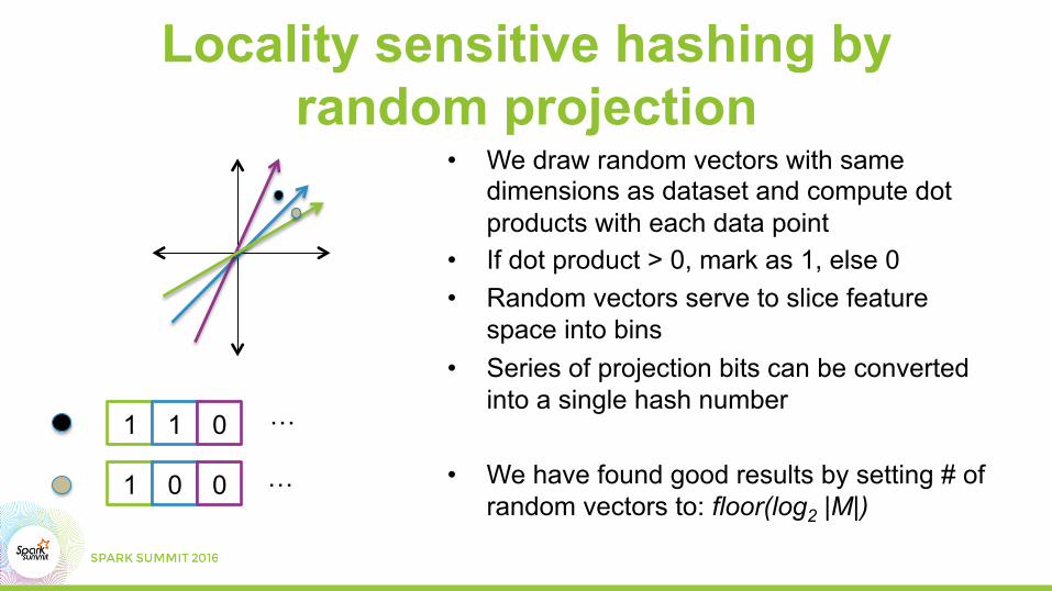
Locality sensitive hashing by random projection
• We draw random vectors with same dimensions as dataset and compute dot products with each data point
• If dot product > 0, mark as 1, else 0 • Random vectors serve to slice feature
space into bins • Series of projection bits can be converted
into a single hash number
• We have found good results by setting # of random vectors to: floor(log2 |M|)
1
1
1
0
0
0
…
…

Scaling with LSH Prototyping on Spark 1. Use Locality Sensitive Hashing
(SimHash / Random Projection) to drop data points into bins
2. Compute “prototype” points for each bin corresponding to bin centroid – can also use median to make
prototyping more robust 3. Use binning information to
compute topological network: distMxM => distBxB, where B is no. of
prototype points (1 per bin)
ü Fastest scalable implementation ü # of random vectors controls # of bins and therefore fidelity of topological representation
ü LSH binning tends to select similar points (inter-bin distance > intra-bin distance)

Betti Mapper
B x B Distance
Matrix of prototypes
M x N
B x 1
B x 1
. . .
. . .
.
. .
. . . . …
LSH
M x M Distance Matrix:
D(p1, p2) = D(bin(p1), bin(p2))
M x 1
M x 1
B x N prototypes
X X
IMPLEMENTATION PERFORMANCE
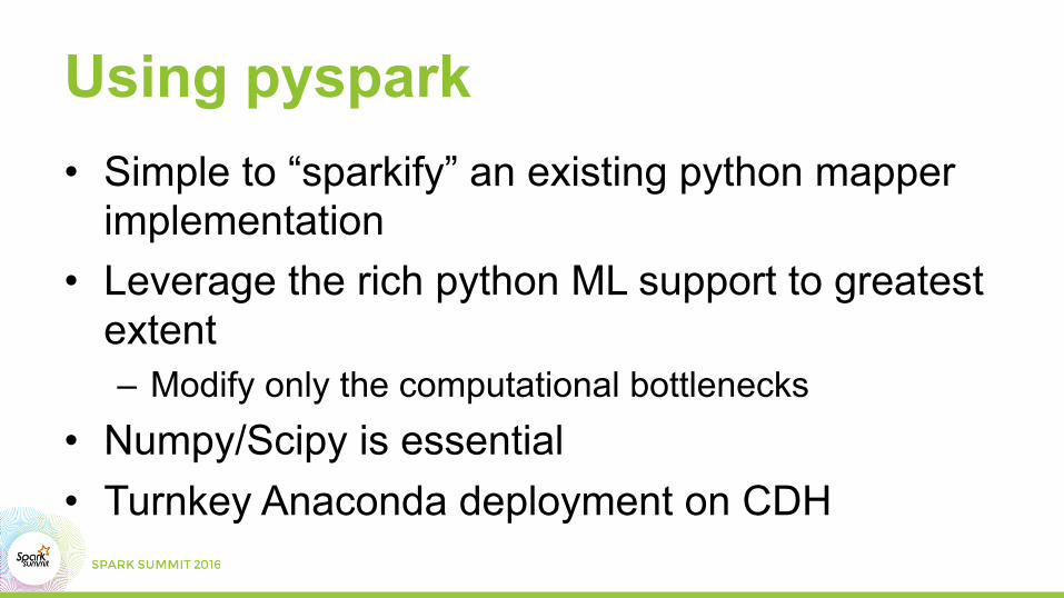
Using pyspark • Simple to “sparkify” an existing python mapper
implementation • Leverage the rich python ML support to greatest
extent – Modify only the computational bottlenecks
• Numpy/Scipy is essential • Turnkey Anaconda deployment on CDH

Naïve performance Ti
me
(Yea
rs) • 4TFLOP/s GPGPU (100% util)
• 5K Columns • Euclidean distance
Seconds
Decades
Row count
0.000
0.000
0.000
0.000
0.000
0.001
0.010
0.100
1.000
10.000
100.000
1000.000
10K 100K 1M 10M 100M 1B
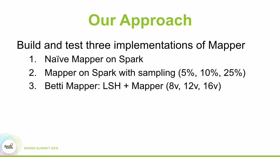
Our Approach Build and test three implementations of Mapper
1. Naïve Mapper on Spark 2. Mapper on Spark with sampling (5%, 10%, 25%) 3. Betti Mapper: LSH + Mapper (8v, 12v, 16v)

Test Hardware
Macbook Pro, mid 2014 • 2.5 GHz Intel® Core i7 • 16 GB 1600 MHz DDR3 • 512 GB SSD
Spark Cluster on Amazon EC2 • Instance type: r3.large • Node: 2 vCPU, 15 GB RAM, 32 GB SSD • 4 workers, 1 driver • 250 GB SSD EBS as persistent HDFS • Amazon Linux, Anaconda 64-bit 4.0.0,
PySpark 1.6.1

Spark Configuration
• --driver-memory 8g • --executor-memory 12g (each) • --executor-cores 2 • No. of executors: 4

Dataset Configuration Filename Size (MxN) Size (bytes) MNIST_1k.csv 1000 rows x 784 cols 1.83 MB MNIST_10k.csv 10,000 rows x 784 cols 18.3 MB MNIST_100k.csv 100,000 rows x 784 cols 183 MB MNIST_1000k.csv 1,000,000 rows x 784 cols 1830 MB
The datasets are sampled with replacement from the original MNIST dataset available for download using Python’s scikit-learn library (mldata module)
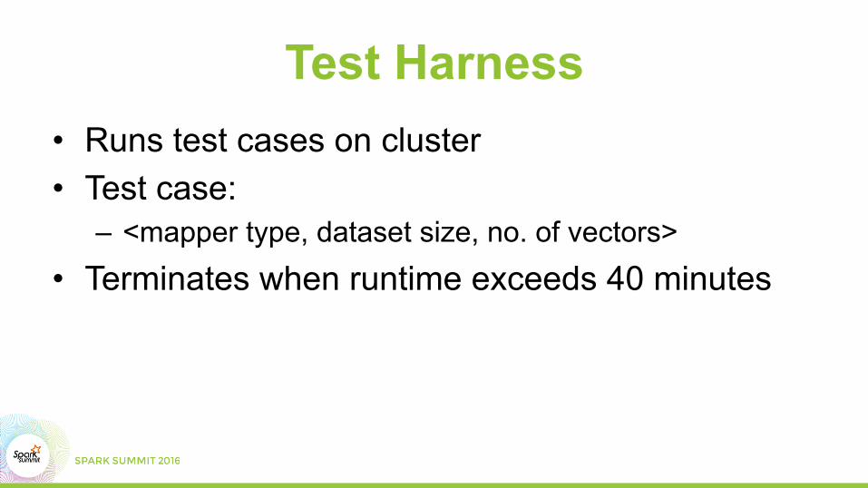
Test Harness • Runs test cases on cluster • Test case:
– <mapper type, dataset size, no. of vectors>
• Terminates when runtime exceeds 40 minutes
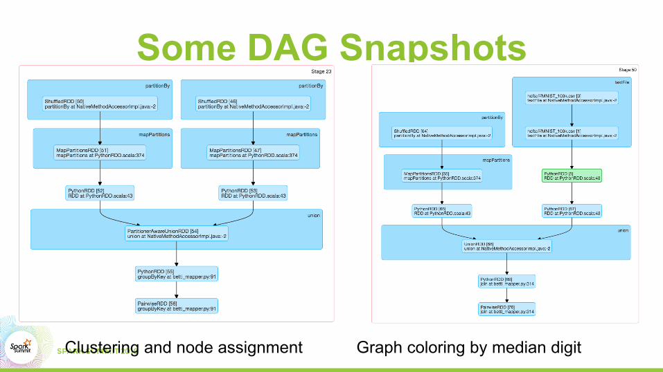
Some DAG Snapshots
Graph coloring by median digit Clustering and node assignment

X X X 40minutes


Future Work • Test other LSH schemes • Optimize Spark code and leverage existing
codebases for distributed linear algebra routines • Incorporate as a machine learning model on the
Alpine Data platform

Alpine Spark TDA
TDA
Key Takeaways • Scaling Mapper algorithm is non-trivial but
possible • Gaining control over fidelity of representation is
key to gaining insights from data • Open source implementation of Betti Mapper will
be made available after code cleanup! J

References • “Topological Methods for the Analysis of High Dimensional Data Sets and 3D
Object Recognition”, G. Singh, F. Memoli, G. Carlsson, Eurographics Symposium on Point-Based Graphics (2007)
• “Extracting insights from the shape of complex data using topology”, P. Y. Lum, G. Singh, A. Lehman, T. Ishkanov, M. Vejdemo-Johansson, M. Alagappan, J. Carlsson, G. Carlsson, Nature Scientific Reports (2013)
• “Online generation of locality sensitive hash signatures”, B. V. Durme, A. Lall, Proceedings of the Association of Computational Linguistics 2010 Conference Short Papers (2010)
• PySpark documentation: http://spark.apache.org/docs/latest/api/python/
Acknowledgements • Rachel Warren • Anya Bida
Alpine is Hiring • Platform engineers • UX engineers • Build engineers • Ping me : [email protected]

Q & (HOPEFULLY) A

THANK YOU. [email protected] [email protected]