envelope condition method with an application to default ...maliarl/files/jedc2016_ammt.pdfbellman...

Contents lists available at ScienceDirect

Journal of Economic Dynamics & Control

Journal of Economic Dynamics & Control 69 (2016) 436–459

http://d0165-18

n CorrE-m

journal homepage: www.elsevier.com/locate/jedc

Envelope condition method with an application to defaultrisk models

Cristina Arellano, Lilia Maliar n, Serguei Maliar, Viktor TsyrennikovOffice 249, Department of Economics, Stanford, CA 94305-6072, USA

a r t i c l e i n f o

Article history:Received 15 February 2013Received in revised form3 May 2015Accepted 19 May 2016Available online 8 June 2016

JEL classification:C6C61C63C68

Keywords:Dynamic programmingBellman equationEndogenous gridCurse of dimensionalityLarge scaleDefault risk

x.doi.org/10.1016/j.jedc.2016.05.01689/& 2016 Elsevier B.V. All rights reserved.

esponding author. Tel.: þ1 6507259069.ail address: [email protected] (L. Maliar)

a b s t r a c t

We develop an envelope condition method (ECM) for dynamic programming problems – atractable alternative to expensive conventional value function iteration (VFI). ECM has twonovel features: first, to reduce the cost of iteration on Bellman equation, ECM constructspolicy functions using envelope conditions which are simpler to analyze numerically thanfirst-order conditions. Second, to increase the accuracy of solutions, ECM solves forderivatives of value function jointly with value function itself. We complement ECM withother computational techniques that are suitable for high-dimensional problems, such assimulation-based grids, monomial integration rules and derivative-free solvers. Theresulting value-iterative ECM method can accurately solve models with at least up to 20state variables and can successfully compete in accuracy and speed with state-of-the-artEuler equation methods. We also use ECM to solve a challenging default risk model with akink in value and policy functions.

& 2016 Elsevier B.V. All rights reserved.

1. Introduction

We develop an envelope condition method (ECM) for dynamic programming problems – a tractable alternative toexpensive conventional value function iteration (VFI). ECM has two novel features: first, to reduce the cost of iteration onBellman equation, ECM constructs policy functions using envelope conditions which are simpler to analyze numericallythan first-order conditions. Second, to increase the accuracy of solutions, ECM solves for derivatives of value function jointlywith value function itself. We complement ECM with other computational techniques that are suitable for high-dimensionalproblems, such as simulation-based grids, monomial integration rules and derivative-free solvers. The resulting value-iterative ECM method can accurately solve models with at least up to 20 state variables and can successfully compete inaccuracy and speed with state-of-the-art Euler equation methods. We finally use ECM to solve a challenging default riskmodel with a kink in value and policy functions.

.

www.sciencedirect.com/science/journal/01651889

www.elsevier.com/locate/jedc

http://dx.doi.org/10.1016/j.jedc.2016.05.016



http://crossmark.crossref.org/dialog/?doi=10.1016/j.jedc.2016.05.016&domain=pdf



mailto:[email protected]



C. Arellano et al. / Journal of Economic Dynamics & Control 69 (2016) 436–459 437

We present ECM in the context of three applications: a one-agent growth model, a multi-country model of internationaltrade and a default risk model. In our first application, we consider a stylized optimal growth model with inelastic laborsupply. To solve such a model, conventional VFI constructs policy function by finding a maximum of the right side of theBellman equation. This is done either directly (by using numerical maximization) or via first-order condition (by using anumerical solver). In contrast, the ECM methods construct policy functions by finding a solution to the envelope condition.Because such a solution can be derived in a closed form, ECM requires only direct calculations and avoids the need of eithernumerical optimization or numerical solvers when iterating on the Bellman equation.

We also develop a version of ECM that approximates derivatives of value function (possibly, jointly with value function)instead of value function itself. This version of ECM produces more accurate solutions than an otherwise identical ECM thatsolves exclusively for value function. This is because solving accurately for value function does not necessarily leads tosufficiently accurate approximations of its derivatives. For example, if value function is approximated with polynomial ofdegree n, then its derivatives are effectively approximated with polynomial of degree n�1, i.e., we ”lose” one polynomialdegree when differentiating value function. In contrast, by approximating derivatives of value function directly, we focus onthe object that identifies policy functions and hence, obtain more accurate solutions.

We then investigate the convergence properties of the constructed class of ECM methods in the context of the studiedoptimal growth model. We establish that ECM has the same fixed point solution as the regular Bellman operator with someadditional technical restriction. However, the ECM operator does not possess the property of contraction mapping like theregular Bellman operator. In this respect, the ECM class of methods is similar to the Euler equation class of methods forwhich global convergence results are generally infeasible. Nevertheless, the fact that the convergence theorems cannot beestablished for some numerical methods does not mean that the method is not useful. In particular, Euler equation methodsare useful in a variety of contexts. In our numerical experiments, the ECM method has good convergence properties andproduces accurate solutions in a wide range of the model's parameters.

In our second application, we construct a version of ECM that is suitable for high-dimensional applications, includingstochastic simulation, non-product monomial integration rules, and derivative-free solvers, to solve a multicountry growthmodel with up to 10 countries (20 state variables).1 This model is the one studied in the February 2011's special issue of theJournal of Economic Dynamics and Control (henceforth, JEDC project) which compares the performance of six state-of-the-art solution methods.2 We show that the ECM methods is tractable and reliable in this setting and is able to successfullycompete with state-of-the-art Euler equation methods in the high-dimensional applications which were part of the JEDCproject. For our most accurate third-degree polynomial solutions, maximum unit-free residuals in the model's equations arealways smaller than 0.002% on a stochastic simulation of 10,000 observations.

Finally, our third application is a default risk model of Arellano (2008). Default models are challenging computationallybecause value and policy functions have kinks and the price function of debt depends on the level of debt reflecting defaultprobabilities. Nonetheless, at the optimal debt level, the decision functions are continuously differentiable and satisfy FOCs;see Clausen and Strub (2013) for a version of the envelope theorem that applies to models with default risk and a survey ofenvelope theorems in the literature. We show that the ECM methods are fast in computing this model. Relative to theexpensive VFI method, ECM speeds up the computation time by more than 50 times. However, the convergence is moredifficult to attain in this model. Numerical errors in approximating value function along iteration may lead to nonmonotonepolicy functions and result in non-convergence. Damping and shape preserving restrictions on value function can help todeal with this problem.

While our analysis is limited to the benchmark default risk model, we think that ECM can be useful for many otherapplications with default risk. In fact, a substantial hurdle for the growing literature on sovereign default is the computa-tional cost; see, e.g., Aguiar and Gopinath (2006), Chatterjee et al. (2007), Hopenhayn and Werning (2008), Bianchi et al.(2009), Maliar et al. (2008), Chatterjee and Eyigundor (2011), Arellano et al. (2013), Tsyrennikov (2013), and Aguiar et al.(2015); see Aguiar and Amador (2013) for a review of the literature on sovereign debt. The ECM methods can facilitate thedevelopment of this literature by expanding the types of problems that can be efficiently solved.

We next discuss the relation of the ECM method to other numerical methods in the literature. Dynamic programmingmethods are introduced in Bellman (1957) and Howard (1960) in the context of stationary, infinite-horizon Markovianproblems. There is a large body of literature that focuses on solving DP problems including methods based on discretizationof state space (e.g., Rust, 1996, 1997), stochastic simulation methods (e.g., Smith, 1991, 1993), Maliar and Maliar, 2005),learning methods (e.g., Bertsekas and Tsitsiklis, 1996), perturbation methods (e.g., Judd, 1998), policy iteration (e.g., Santosand Rust, 2008), nonexpensive approximations (Stachurski, 2008), approximate DP methods (e.g., Powell, 2011), polyhedralapproximations (e.g., Fukushima andWaki, 2011), random contractions (Pal and Stachurski, 2013); also see Rust (2008), Judd(1998), Santos (1999), and Stachurski (2009) for literature reviews. From one side, many methods, which are accurate andreliable in problems with low dimensionality, are intractable in problems with high dimensionality. This is in particular true

1 See Maliar and Maliar (2014) for a survey of these and other numerical techniques that are tractable in problems with a large number of statevariables.

2 The objectives of the JEDC project are described in Den Haan et al. (2011); the methodology of the numerical analysis is outlined in Juillard andVillemot (2011); the results of the comparison analysis are provided in Kollmann et al. (2011b). The six participating methods are first- and second-orderperturbation methods of Kollmann et al. (2011a), stochastic simulation and cluster-grid algorithms of Judd et al. (2011), monomial rule Galerkin method ofPichler (2011) and Smolyak's collocation method of Malin et al. (2011).

C. Arellano et al. / Journal of Economic Dynamics & Control 69 (2016) 436–459438

for projection-style methods that rely on tensor product rules in the construction of either grid points or integration nodes.From the other side, methods that are tractable in high-dimensional problems may be insufficiently accurate. One exampleis perturbation methods whose accuracy deteriorates rapidly away from the steady state. Another example is simulation-based methods, including approximate DP methods and learning methods, whose accuracy is limited by a low (square-root)rate of convergence of Monte Carlo simulation, see Judd et al. (2011). In contrast to such methods, ECM relies on accuratedeterministic integration methods and is both tractable and accurate in problems with high dimensionality.

Endogenous grid method (EGM) of Carroll (2005) reduces the cost of conventional VFI; see also Barillas and Fernandez-Villaverde (2007) and Ishakov et al. (2012). In a companion paper, Maliar and Maliar (2013) compare the ECM and EGMmethods in the context of a one-agent model with elastic labor supply and find that the two methods are very similar bothin terms of accuracy of solutions and computational expense. However, in more complex applications, one method mayhave advantages over the other. Constructing a grid on future state variables under EGM is complicated in problems withkinks in future state variables (due to, e.g., occasionally binding inequality constraints or default) because it is not known atthe stage of initialization whether an inequality constraint binds or whether a default occurs in a given grid point. Thistypically requires to nest the EGM method within another iterative procedure; see, e.g., Villemot (2012) and Fella (2014). Incontrasts, ECM methods use the conventional current state variables and may be easier to implement.

Other papers that solve high-dimensional problems are multicountry models with 20–60 state variables in Judd et al.(2011, 2012, 2014); medium-scale new Keynesian models in Judd et al. (2011, 2012), Fernández-Villaverde et al. (2012),Aruoba and Schorfheide (2013), Gust et al. (2012) Maliar and Maliar (2015), etc.; and large-scale OLG models with up to 80state variables in Hasanhodzic and Kotlikoff (2013). All the methods that solve high-dimensional problems, including thoseparticipating in the JEDC project, build on Euler equations, and none of these papers uses value iterative approaches evenwhen the studied models admit a dynamic programming representation. However, value iterative approaches that build onECM can successfully compete with state-of-the-art Euler equation methods in high-dimensional applications.3 In particular,we are able to compute accurate polynomial approximations up to third degree, while the Euler equation methods parti-cipating in the comparison analysis of Kollmann et al. (2011b) are limited to less accurate second-degree polynomials (dueto their high computational expense).

The rest of the paper is organized as follows. In Section 2, we illustrate the ECM methods in the context of the standardone-agent neoclassical growth model. In Section 3, we apply the ECM methods to solve the multicountry growth modelsstudied in the JEDC project. In Section 4, we apply the ECM method to solve a default risk model. In Section 5, we conclude.

2. ECM in the one-agent growth model

We begin by illustrating the envelope condition method (ECM) in the context of the standard one-agent neoclassicalgrowth model.

2.1. The model

We consider a dynamic programming (DP) problem of finding value function, V, that solves the Bellman equation,

V k; zð Þ ¼maxc;k0

u cð ÞþβE V k0; z0� �� ð1Þ

s:t: k0 ¼ 1�δð Þkþzf kð Þ�c; ð2Þ

ln z0 ¼ ρ ln zþε0; ε0 �N 0; σ2� �

; ð3Þwhere k, c and z are capital, consumption and productivity level, respectively; βA 0;1ð Þ; δA 0;1ð �; ρA �1;1ð Þ; σZ0; theutility and production functions, u and f, respectively, are strictly increasing, continuously differentiable and strictly concave.The primes on variables denote next-period values, and E V k0; z0

� �� is an expectation conditional on state k; zð Þ.

2.2. First order condition (FOC) versus envelope condition (EC)

Under our assumptions, a solution to Bellman equation (1)–(3) exists, is interior and is unique; and optimal valuefunction V is differentiable, strictly increasing and strictly concave; see Stokey and Lucas with Prescott (1989), Santos (1999)and Stachurski (2009) for a discussion. We compute the derivative of V in the left side of (1) to obtain

V1 k; zð Þ ¼ u0 C k; zð Þð ÞC1 k; zð ÞþβE V1 K k; zð Þ; z0ð Þ� �K1 k; zð Þ; ð4Þ

where c¼ C k; zð Þ and k0 ¼ K k; zð Þ are the optimal policy functions. (Here and further in the paper, Fi …; xi;…ð Þ denotes a first-order partial derivative of function F …; xi;…ð Þ with respect to ith variable xi).

3 In a recent contribution, Achdou et al. (2015) show how to apply the envelope type of argument for constructing numerical solutions to dynamiceconomic models in continuous time, including heterogeneous agent models.


According to (2), we have C1 k; zð Þ ¼ 1�δþzf kð Þ�K1 k; zð Þ. Substituting the latter result into (4) yields

V1 k; zð Þ�u0 C k; zð Þð Þ 1�δþzf 0 kð Þ� �|fflfflfflfflfflfflfflfflfflfflfflfflfflfflfflfflfflfflfflfflfflfflfflfflfflfflfflfflfflfflffl{zfflfflfflfflfflfflfflfflfflfflfflfflfflfflfflfflfflfflfflfflfflfflfflfflfflfflfflfflfflfflffl}EC

¼ βE V1 k0; z0� �� u0 C k; zð Þð Þ� �|fflfflfflfflfflfflfflfflfflfflfflfflfflfflfflfflfflfflfflfflfflfflfflfflffl{zfflfflfflfflfflfflfflfflfflfflfflfflfflfflfflfflfflfflfflfflfflfflfflfflffl}

FOC

K1 k; zð Þ: ð5Þ

The left side of (5) is the envelope condition (EC) and the right side corresponds to first order condition (FOC) of themaximization problem (1)–(3).

Conventional value function iteration (VFI) and policy iteration (PI) construct policy functions such as consumptionfunction by setting the FOC equal to zero (we denote such a function by CFOC k; zð ÞÞ:

u0 CFOC k; zð Þð Þ ¼ βE V1 k0; z0� ��

: ð6ÞIn contrast, the class of methods advocated in the present paper solves for consumption function by setting the EC equal tozero (we denote such a function by CEC k; zð ÞÞ:

V1 k; zð Þ ¼ u0 CEC k; zð Þð Þ 1�δþzf 0 kð Þ� �: ð7Þ

We refer to this new class of methods as envelope condition methods (ECM), following Maliar and Maliar (2013).In the true solution, both ways of constructing the consumption function, defined by (6) and (7), must lead to the same

consumption function since the solution must satisfy both the FOC and EC, i.e., CFOC ¼ CEC . However, operationally, the con-struction of CEC from (7) is simple (namely, CEC can be derived in a closed form), whereas the construction of CFOC from (6) ismore complicated (it generally involves using a numerical solver). Replacing FOC with EC leads to a dramatic reduction in cost ofvalue iteration, as the policy functions must be constructed a large number of times along iteration; see Maliar and Maliar (2013)for numerical examples. However, it turned out that the new way of constructing policy functions affects also the convergenceproperties of VFI and PI methods. In the remainder of the paper, we formulate several different variants of the ECM methods,explore their convergence properties, discuss their relation to the literature and illustrate their applications with examples.

2.3. Value function iteration

We now describe a variant of ECM that finds a solution to Bellman equation by iterating on value function and wecompare it to two related methods in the literature, conventional value function iteration and endogenous grid method ofCarroll (2005).

2.3.1. ECM-VFECM-VF finds consumption from envelope condition (7). It constructs value function V satisfying (1)–(3) by the following

iteration procedure:

Algorithm 1. ECM-VF.
Given V, for each point k; zð Þ, define the following recursion:
(i) Find c¼ u0�1 V1 k;zð Þ1� δþ zf 0 kð Þ

h i.

(ii) Find k0 ¼ 1�δð Þkþzf kð Þ�c.

(iii) Find bV k; zð Þ ¼ u cð ÞþβE V k0 ; z0� ��

.

Iterate on (i)–(iii) until convergence bV ¼ V .

The formulas in (i) and (ii) are envelope condition (7) and budget constraint (2), respectively, and the formula in (iii) isBellman equation (1), evaluated under optimal policy functions (which eliminates the maximization sign). We observe thatunder ECM-VF, neither numerical maximization nor numerical solver is necessary for iteration on the Bellman equation butjust direct calculations. The envelope condition type of argument is used in Achdou et al. (2015) to construct a new class offast and efficient numerical methods for solving dynamic economic models in continuous time.

2.3.2. Conventional VFI and EGMTwo related methods in the literature are conventional VFI and endogenous grid method (EGM) of Carroll (2005). Both

methods perform time iteration on FOC (6), namely, they guess value function at tþ1 and use the Bellman equation tocompute value function at t. FOC (6), combined with budget constraint (2), becomes

u0 cð Þ ¼ βE V1 1�δð Þkþzf kð Þ�c; z0ð Þ� �: ð8Þ

Conventional VFI finds consumption from FOC (8).

Algorithm 2. Conventional VFI.
Given V, for each point k; zð Þ, define the following recursion:
(i) Solve for c satisfying u0 cð Þ ¼ βE V1 1�δð Þkþzf kð Þ�c; z0ð Þ� �.




.


Conventional VFI is expensive because step (i) requires us to numerically find a root to (8) for each k; zð Þ by interpolatingV1 to new values k0; z0

� �and by approximating conditional expectation – this all must be done inside an iterative cycle; see

Aruoba et al. (2006) for an example of cost assessment of conventional VFI (alternatively, we can find k0 by maximizing theright side of Bellman Eq. (1) directly without using FOCs, however, this is also expensive).

Carroll (2005) proposes a way to reduce the cost of conventional VFI. The EGM method of Carroll (2005) exploits the factthat it is easier to solve (8) with respect to c given k0; z

� �than to solve it with respect to c given k; zð Þ. EGM constructs a grid

on k0; z� �

by fixing the future endogenous state variable k0 and by treating the current endogenous state variable k asunknown. Since k0 is fixed, EGM computes E V1 k0; z0

� �� up-front and thus can avoid costly interpolation and approximation

of expectation in a rootfinding procedure.

Algorithm 3. EGM of Carroll (2005).

Given V, for each point k0 ; z� �

, define the following recursion:

(i) Find c¼ u0�1 βE V1 k0 ; z0� ��

.

(ii) Solve for k satisfying k0 ¼ 1�δð Þkþzf kð Þ�c.


.


In step (ii) of EGM, we still need to find k numerically. However, for the studied model, Carroll (2005) shows a change ofvariables that makes it possible to avoid finding k numerically on each iteration (except of the very last iteration).

As we have seen, ECM-VF avoids the rootfinding completely in the studied model (even without a change of variables).Thus, it attains the same outcome as the EGM of Carroll (2005) via a different mechanism. In more complicated models, forexample, an optimal growth model with elastic labor supply, neither EGM nor ECM avoid the rootfinding completely butstill simplify it considerably compared to conventional VFI; see Barillas and Fernandez-Villaverde (2007) for an extension ofEGM to a model with elastic labor supply. In a companion paper, Maliar and Maliar (2013) show that ECM-VF and EGMperform very similarly in terms of their accuracy and speed in the context of a model with elastic labor supply.

However, EGM of Carroll (2005) is non-trivial to implement for models in which future state variables have kinks, forexample, for models with occasionally binding inequality constraints or with a risk of default. Since EGM needs to constructa grid on future state variables, we must specify whether an inequality constraint binds or whether a default occurs in eachgrid point. This is generally not possible to do before the model is solved. To deal with this complication, the literature nestsEGM within another iterative procedure; see, e.g., Villemot (2012) and Fella (2014). The proposed ECM methods may haveadvantages over EGM for this kind of problems as they construct grids on present state variables whose values are naturallyknown. In Section 4, we apply an ECM method to solve a default risk model.

2.4. Policy iteration

We now describe a variant of ECM that solves Bellman equation by iterating on policy function and we compare it toconventional PI methods, e.g., Santos and Rust (2008); see Santos and Rust (2008), Rust (2008) and Stachurski (2009) for ageneral discussion of policy iteration methods.

2.4.1. ECM-PIWe refer to a variant of ECM that performs PI instead of VFI as ECM-PI.

Algorithm 4. ECM-PI.
Given C, for each point k; zð Þ, define the following recursion:
(i) Find K k; zð Þ ¼ 1�δð Þkþzf kð Þ�C k; zð Þ.(ii) Solve for V satisfying V k; zð Þ ¼ u C k; zð Þð ÞþβE V K k; zð Þ; z0ð Þ� �

.

(iii) Find bC k; zð Þ ¼ u0�1 V1 k;zð Þ1�δþ zf 0 kð Þ

h i.

Iterate on (i)–(iii) until convergence bC ¼ C.

That is, the ECM-PI method guesses policy function for consumption c¼ C k; zð Þ, finds the corresponding policy function forcapital k¼ K k; zð Þ, computes the corresponding V by iteration on the Bellman equation until convergence holding the policyfunctions fixed and recomputes the policy function bC k; zð Þ, iterating until convergence. An example of ECM iterating onpolicy function is shown in Section 4.2.1.


2.4.2. Conventional policy iterationConventional policy iteration methods construct consumption function using FOC (6) instead of envelope condition (7).

Algorithm 5. Conventional PI.
Given C, for each point k; zð Þ, define the following recursion:
(i) Find K k; zð Þ ¼ 1�δð Þkþzf kð Þ�C k; zð Þ.(ii) Solve for V satisfying V k; zð Þ ¼ u C k; zð Þð ÞþβE V K k; zð Þ; z0ð Þ� �

.

(iii) Find bC satisfying u0 bC k; zð Þ

¼ βE V1 1�δð Þkþzf kð Þ� bC k; zð Þ; z0 h i

.


The difference between ECM-PI and conventional PI consists in step (iii) in which the policy function for next iteration isconstructed.

2.5. Iteration on derivatives of value function

The ECM methods described up to now solve for value function (either directly or via PI). We now describe versions ofECM that solve for derivative of value function instead of value function itself. We argue that the derivative-based version ofECM has similarity to the Euler-equation class of methods.

2.5.1. ECM-DVFThe studied ECM method suggests a useful recursion for the derivative of value function. We first construct consumption

function C k; zð Þ satisfying FOC (6) under the current value function βE V1 k0; z0� �� ¼ u0 C k; zð Þð Þ, and we then use (4) to obtain

the derivative of value function for next iteration:

V1 k; zð Þ ¼ β 1�δþzf 0 kð Þ� �E V1 k0; z0

� �� : ð9Þ

This leads to a solution method that we call ECM-DVF.

Algorithm 6. ECM-DVF.
Given V1 for each point k; zð Þ, define the following recursion:
(i) Find c¼ u0�1 V1 k;zð Þ1� δþ zf 0 kð Þ

h i.


(iii) Find bV 1 k; zð Þ ¼ β 1�δþzf 0 kð Þ� �E V1 k0 ; z0

� �� .

Iterate on (i)–(iii) until convergence bV 1 ¼ V1.Given the converged policy functions, find V satisfying V k; zð Þ ¼ u cð ÞþβE V k0 ; z0

� �� :

The difference of ECM-DVF from the previously studied ECM-VF consists in that we iterate on V1 without computing V oneach iteration. We only compute V at the very end, when both V1 and the optimal policy functions are constructed. Again,neither numerical maximization nor a numerical solver is necessary under ECM-DVF but only direct calculations.

In our numerical experiments, a version of ECM-DVF that solves for a derivative of value function produces more accuratesolutions than an otherwise identical ECM-VF that solves exclusively for value function. This is because solving accuratelyfor value function does not lead to sufficiently accurate approximations of its derivatives. For example, assume that valuefunction is approximated with polynomial of degree n. Then, its derivatives are effectively approximated with a polynomialof degree n�1 since we “lose” one polynomial degree when differentiating value function. In contrast, when approximatingderivatives of value function directly, we focus on the object that identifies policy functions and as a result, we obtain moreaccurate solutions.

Maliar and Maliar (2013) also show how to construct a version of EGM-DVF of Carroll (2005) that iterates on thederivatives of value function instead of the value function itself in a way that is parallel to ECM-DVF. This paper finds that theperformance of ECM-DVF and EGM-DVF is very similar in terms of their accuracy and speed in the context of a model withelastic labor supply. Finally, it is straightforward to formulate the variants of ECM-DVF and ECM-DVF that perform PI insteadof VFI but we omit this extension to save on space.

2.5.2. Euler equation methodsECM-DVF has similarity to Euler equation methods; see Judd (1998) and Santos (1999) for a general discussion of such

methods. The standard Euler equation follows from optimality conditions (6) and (7): we update (7) to obtain V1 k0; z0� �

andwe substitute the result into (6) to eliminate the unknown derivative of the value function,

u0 cð Þ ¼ βE u0 c0ð Þ 1�δþz0f 0 k0� ��

: ð10ÞEuler equation methods approximate policy functions for consumption c¼ C k; zð Þ, capital k0 ¼ K k; zð Þ (or other policy


functions) to satisfy (2), (3) and (10). Below, we provide an example of Euler equation method (other recursions for suchmethods are possible).

Algorithm 7. Euler equation algorithms.
Given C k; zð Þ, for each point k; zð Þ, define the following recursion:
(i) Find K k; zð Þ ¼ 1�δð Þkþzf kð Þ�C k; zð Þ.(ii) Find c0 ¼ C K k; zð Þ; z0ð Þ.(iii) Find bC k; zð Þ ¼ u0�1 βE u0 c0ð Þ 1�δþz0f 0 k0

� �� .


Similar to ECM, Euler equation methods do not solve for value function but only for decision (policy) functions. Onepossible decision function is a derivative of value function. Thus, the ECM recursion (9) can be also viewed as an Eulerequation written in terms of the derivative of value function.

2.6. Convergence properties of the ECM methods

We now study the convergence of the ECM methods. For the expositional convenience, our analysis is limited to theoptimal growth model (1)–(3), however, it can be readily extended to other models that satisfy the standard assumptionssuch as compactness and convexity of the budget set, smoothness and strong concavity of the utility function and theinteriority of solutions; see Stokey and Lucas with Prescott (1989), Santos (1999, 2000), Stachurski (2009) and Krueger(2012) for a discussion of these assumptions.

2.6.1. ECM-VFWe study the convergence of the ECM method iterating on value function, described in Section 2.3.1; see “Algorithm 1

ECM-VF”. Our analysis relies on the comparison of ECM to the conventional VFI iteration; see “Algorithm 2 FOC-VFI”. Wedefine the regular Bellman operator T for the model (1)–(3) as

TV k; zð Þ � u CFOC k; zð Þð ÞþβE V zf kð Þ�CFOC k; zð Þ; z0ð Þ� �; ð11Þ

CFOC k; zð Þ:u0 cð Þ ¼ βE V1 zf kð Þ�c; z0ð Þ� �; ð12Þ

where CFOC k; zð Þ is the consumption function defined implicitly by FOC (6) (to simplify the notation, we assume δ¼ 1 in thissection).

We next introduce an operator Q that corresponds to the ECM-VF recursion

QV k; zð Þ � u CEC k; zð Þð ÞþβE V zf kð Þ�CEC k; zð Þ; z0ð Þ� �; ð13Þ

CEC k; zð Þ:V1 k; zð Þ ¼ u0 cð Þzf 0 kð Þ; ð14Þwhere CEC k; zð Þ is the consumption function defined implicitly by envelope condition (7).

Does ECM-VF have the same fixed point as conventional VFI? The operators T and Q are different but any fixed point of T isalso a fixed point of Q and vice versa (with an additional technical restriction). Specifically, we have the following result.

Proposition 1. Let Vn be a fixed point of Q such that K1a0. Than, V� ¼ TV� iff V� ¼QV�.

Proof. The proof follows by formula (5) that shows that imposing FOC enforces the envelope condition and vice versa.(i) To see that V� ¼ TV� implies V� ¼QV�, note that if Vn is a fixed point of T, then assuming interiority, CFOC must satisfy

FOC (12). Hence, according to (5), CFOC must also satisfy envelope condition (14). Hence, CFOC ¼ CEC and hence, V� ¼ QV�.(ii) In the opposite direction, note that if Vn is a fixed point of Q, then CEC satisfies envelope condition (14). According to (5),

CEC must either satisfy FOC (12) or it must be the case that K1 ¼ 0. Since the latter possibility is ruled out by assumption, weconclude that CFOC ¼ CEC . Hence, V

� ¼QV� implies V� ¼ TV�. □

The restriction K1a0 is important and allows us to rule out degenerate functions that satisfy envelope condition but notFOC and hence, that are not solutions to the Bellman equation. We illustrate this point by way of example.

Example 1. Assume u 0ð Þ ¼ f 0ð Þ ¼ 0 and consider V k; zð Þ ¼ u zf kð Þð Þ. According to (14), we have

CEC k; zð Þ ¼ u0�1 V1 k; zð Þzf 0 kð Þ

� �¼ u0�1 u0 zf kð Þð Þzf 0 kð Þ

zf 0 kð Þ

� �¼ zf kð Þ:

Inserting this result in the right side hand side of (13), we have

QV k; zð Þ ¼ u CEC k; zð Þð ÞþβE V zf kð Þ�CEC k; zð Þ; z0ð Þ� �u zf kð Þð ÞþβE V zf kð Þ�zf kð Þ; z0ð Þ� �¼ u zf kð Þð ÞþβE V 0; z0ð Þ½ � ¼ u zf kð Þð Þ


Hence, V k; zð Þ ¼ u zf kð Þð Þ is a fixed point of Q which is not fixed point of T. This is a degenerate fixed point that has capitalfunction K¼0 that does not satisfy the restriction K1 ¼ 0. □

Does ECM-VF have the contraction mapping property as conventional VFI? Our goal is to analyze the convergence propertiesof ECM-VF. In order to do this, it is useful to recall the convergence results for the regular Bellman operator T. It is well-known that the Bellman operator is a contraction mapping and thus, it guarantees a convergence to a fixed point Vn startingfrom an arbitrary initial guess V, in the space of continuous bounded functions, i.e., TnV-V� as n-1. The proof of this factis as follows:

Let V and W be two continuous bounded functions. Then, we have

TV k; zð Þ�TW k; zð Þ ¼ max

cu cð ÞþβE V zf kð Þ�c; z0ð Þ� �� max

cu cð ÞþβE W zf kð Þ�c; z0ð Þ� �� :

Using the property of a maximum operator, we obtain

TV k; zð Þ�TW k; zð Þ rmax

cu cð ÞþβE V zf kð Þ�c; z0ð Þ� �� u cð ÞþβE W zf kð Þ�c; z0ð Þ� �� :

Taking the supremum on the left-hand side shows that T is a contraction mapping with a modulus β,

TV�TWk krβ V�Wk k; ð15Þwhere here and further in the text �k k is used to denote the supremum L1 norm.

We next ask: Is the ECM-VF operator Q a contraction mapping like T? In other words, does Q guarantee a convergence toa fixed point QnV-V� as n-1 in the space of continuous bounded functions? Example 1 suggests a negative answer to thisquestion. Indeed, if we use V k; zð Þ ¼ u zf kð Þð Þ for initializing ECM-VF (such a guess is frequently used for initializing con-ventional VFI in applications), ECM-VF will get stuck in a wrong fixed point with K¼0. Clearly, ECM-VF does not guarantee aconvergence from any initial guess.

To further explore the convergence properties of ECM-VF, let us repeat the same steps for this method as we did for theregular Bellman operator. We have

QV k; zð Þ�QW k; zð Þ ¼ u cV k; zð Þð ÞþβE V zf kð Þ�cV k; zð Þ; z0ð Þ� ��u cW k; zð Þð Þ�βE W zf kð Þ�cW k; zð Þ; z0ð Þ� � ; ð16Þ

where cV k; zð Þ and cW k; zð Þ are consumption functions generated by the envelope conditions of V and W, respectively,

cV k; zð Þ:V1 k; zð Þ ¼ u0 cð Þzf 0 kð Þ;cW k; zð Þ:W1 k; zð Þ ¼ u0 cð Þzf 0 kð Þ: ð17Þ

By using a triangular inequality and by taking a supremum of (16), we arrive at

QV�QWk kr‖u cVð Þ�u cWð Þ‖þβ V�Wk k: ð18ÞFormula (18) for the ECM operator Q has a new term u cVð Þ�u cWð Þ

�� compared to a similar formula (15) for the regularBellman operator T. This term can be potentially large if the derivatives of V and W are very different, and hence, the ECMoperator Q is not necessarily a contraction mapping.

To investigate the convergence properties of the term u cVð Þ�u cWð Þ�� , we study the recursion that ECM implies for the

derivative V1. On iteration n, we first construct consumption function Cn k; zð Þ satisfying envelope condition (7) under thecurrent value function Vn

1 k; zð Þ ¼ u0 Cn k; zð Þ� �1�δþzf 0 kð Þ� �

, and we then use (5) to obtain following recursion for the deri-vative of value function for iteration nþ1:

Vnþ11 k; zð Þ ¼ Vn

1 k; zð Þþ βE Vn1 k0; z0� �� Vn

1 k; zð Þ1�δþzf 0 kð Þ

� �Kn1 k; zð Þ: ð19Þ

With the result (19), we obtain the following equation that describes the evolution of Cn k; zð Þ along iteration for the ECM-VFmethod:

u0 Cnþ1 k; zð Þ

¼ u0 Cn k; zð Þ� �þ βE u0 Cn k0; z0� ��

z0f 0 k0� �� u0 Cn k; zð Þ� �� Kn

1 k; zð Þzf 0 kð Þ : ð20Þ

Effectively, the recursion (20) attempts to solve an Euler equation

u0 Cn k; zð Þ� �¼ βE u0 Cn k0; z0� ��

z0f 0 k0� �� ð21Þ

using fixed point iteration. However, the convergence of fixed point iteration on Euler equation is not generally guaranteed;see Maliar and Maliar (2014) for a discussion. The absence of strong convergence results is an important shortcoming of theclass of Euler equation methods relative to the class of conventional value-iterative approaches.

Why do the Bellman and ECM operators have different convergence properties? Note that a solution to EC (7) does notmaximize the right side of the Bellman equation for any V that occurs in iteration (it only does for a limiting fixed-pointsolution Vn). Similarly, the regular Bellman operator enforces FOC (6) in each iteration but does not enforces envelopecondition (7); it only enforces such a condition in the limiting fixed point Vn. Since ECM does not produce a maximum of the


Bellman equation in each iteration, it is not possible to cancel out u cVð Þ�u cWð Þ�� , as is possible to do under the regular

Bellman operator. This fact prevents us from having the property of contraction mapping.

2.6.2. ECM-PIGlobal convergence for policy iteration is established for a space of concave value functions in Santos and Rust (2008).

Thus, the convergence of policy iteration methods requires more stringent conditions than the convergence of the regularBellman operator that is established for a more general class of continuous bounded functions.

Unfortunately, the restriction of concavity of value function is still not sufficient to insure the convergence of ECM-PI.This is because ECM-PI is subject to the same shortcomings as ECM-VF. Namely, the conventional PI method computespolicy functions to satisfy FOC (21) exactly on each iteration, while the ECM-PI method again applies fixed-point iteration(20) to solve FOC only in the limit. This fact can be seen by comparing Algorithms 4 and 5 which have identical steps 1 and2 but differ in step 3.

2.6.3. ECM-DVFWe next turn to ECM-DVF methods described in Section 2.2.2, specifically, we consider the recursion ECM-DVF (9) that is

used in Algorithm 7. We introduce an operator D that corresponds to the ECM-DVF recursion as follows:

DV1 k; zð Þ � zf 0 kð ÞβE V1 zf kð Þ�cV k; zð Þ; z0ð Þ� �; ð22Þ

cEC k; zð Þ:V1 k; zð Þ ¼ u0 cð Þzf 0 kð Þ: ð23ÞWe investigate the convergence properties of the ECM-DVF operator as we did for ECM-VF. Let V1 and W1 be two boundedcontinuous functions. Then, we have

jDV1ðk; θÞ�DW1ðk; θÞj ¼ zf 0 kð Þ β EV1 zf kð Þ�cV k; zð Þ; z0ð Þ� ��EW1 zf kð Þ�cW k; zð Þ; z0ð Þ� � :By taking a supremum, we obtain

DV1�DW1k krzf 0 kð Þβ V1�W1k k: ð24ÞTo have a contraction mapping, we need the term zf 0ðkÞβ in (24) to be smaller than 1 for all k; zð Þ. However, this is not thecase: this term is equal to 1 in the steady state, and it is either smaller or larger than 1 depending on a specific state k; zð Þconsidered.

Another possible way to prove that a mapping is contraction is to show that it satisfies Blackwell's (1965) sufficiencyconditions; see Santos (1999) and Stachurski (2009) for a discussion of these conditions. It is easy to check that the operatorECM-DVF possesses the property of monotonicity but not discounting which agrees with the result (24) (curiously, for thepreviously considered operator ECM-VF (13) and (14), we find exactly the opposite, namely, it possesses the property ofdiscounting but may fail to satisfy monotonicity). Hence, our theoretical analysis does not provide a basis to affirm thatECM-DVF (22) is a contraction mapping.

2.6.4. DiscussionConventional VFI and PI are classified as DP methods. An important advantage of the DP class of methods is that under

the appropriate assumptions, their properties can be characterized analytically including their convergence rates, errorbounds, numerical stability and computational complexity; see Stokey and Lucas with Prescott (1989), Santos (1999) andStachurski (2009) for reviews of formal results for such methods.

In turn, the ECM method solves for value and/or policy functions jointly and effectively includes iteration on Eulerequation. For the Euler equation class of methods, formal results are harder to obtain and even their convergence is ingeneral not guaranteed. Effectively, we need to find a numerical solution to a system of non-linear equations. There are threeapproaches in the literature that are used to solve non-linear systems of equations, namely, fixed point iteration, timeiteration, and Newton-style solvers; see Maliar and Maliar (2014) for a discussion. Time iteration is a special kind of fixedpoint iteration that mimics the Bellman operator: given a guess about decision functions for future variables, it finds thevalues of the current variables to update the guess, iterating until convergence. Time iteration is more numerically stablethan other fixed point iteration schemes, however, it is also more expensive; see Judd (1998, Chapter 16) for a discussion.Moreira and Maldonado (2003) show a variant of the time-iteration method for deterministic problems that is a contractionmapping. The idea is to construct a sequence of subiterations on the Euler equation by exploiting a local saddle-pathstability of the system. Another paper that shows convergence results for their Euler equation method is Feng et al. (2009).

The ECM class of methods is not related to a specific iterative procedure for finding a fixed point and is compatible withall the procedures discussed above. In our numerical experiments, we use fixed point iteration with damping because it issimple, inexpensive and reliable. Instead, we could have used time iteration or Newton-style solvers. For a version of theECM-DVF method based on time iteration, we can possibly show (local) convergence by using a construction similar to theone in Moreira and Maldonado (2003). However, the latter paper is limited to deterministic settings. Generalizing theiranalysis to a stochastic case is a non-trivial task and it goes beyond the scope of the present paper. We leave this extensionfor further research.


Finally, we shall emphasize that the absence of convergence results for Euler equation methods does not mean that suchmethods diverge and are not useful. Euler equation methods successfully converge in many applications under an appro-priate implementation although we cannot prove it analytically. Moreover, even if iteration on Euler equation becomesexplosive, it can often be stabilized by damping; see Maliar et al. (2011) for a graphical illustration. The same is true for theECM class of methods advocated in the present paper.

2.7. Numerical analysis

We now present the results of numerical experiments for the one-agent model.

2.7.1. Computational choicesWe parameterize the model (1)–(3) using the Constant Relative Risk Aversion (CRRA) utility function, u cð Þ ¼ c1� γ �1

1� γ , andthe Cobb–Douglas production function, f kð Þ ¼ kα, and we calibrate the parameters to the standard values: α¼ 1=3, β¼ 0:99,δ¼ 0:025, ρ¼ 0:95 and σ ¼ 0:01. We consider two values of risk-aversion coefficient γ ¼ 1=3 and γ ¼ 3. As a solution domain,we use a rectangular, uniformly spaced grid of 10�10 points for capital and productivity within an ergodic range (todetermine such a range we solve and simulate the model several times). We use a 10-node Gauss–Hermite quadrature rulefor approximating integrals. We parameterize value function (ECM-VF) or a derivative of value function (ECM-DVF) withcomplete ordinary polynomials of degrees up to 5. As an initial guess, we use a linear approximation to the capital policyfunction. To solve for the polynomial coefficients, we use fixed point iteration. We use MATLAB software, version 7.6.0.324(R2012a) and a desktop computer ASUS with Intel(R) Core(TM)2 Quad CPU Q9400 (2.66 GHz), RAM 4 MB. A detaileddescription of the algorithms is provided in Appendix A.

2.7.2. ResultsIn Table 1, we show the results for the ECM-VF. As a measure of accuracy, we report the average and maximum absolute unit-

free residuals in Euler equation (10). Furthermore, in Table 2, we report the results for the ECM-DVF under the same para-meterizations. The main finding is that both ECM-VF and ECM-DVF deliver high accuracy levels. The accuracy increases with adegree of approximating polynomial. ECM-VF is less accurate than ECM-DVF given the same degree of approximating polynomial.This is because if we approximate V with polynomial of some degree, we effectively approximate V1 with polynomial of onedegree less, i.e., we “lose” one polynomial degree. When γ increases (decreases), the accuracy of solutions decreases (increases);these cases are not reported. Namely, under γ ¼ 3 (γ ¼ 1=3), the residuals for ECM-VF vary with the polynomial degree from �3.2to �6.04 (resp., from �3.83 to �7.51). For ECM-DVF, the corresponding residuals vary from �2.98 to �6.63 (resp., from �3.59 to�8.44).

Finally, as we see from the table, the convergence of ECM-VF is faster than that of ECM-DVF. The observed difference incosts represents the difference in the number of iterations necessary for convergence. ECM-DVF needed more iterations toconverge because it was less numerically stable than ECM-VF, and we stabilize it using damping with an updating rate of10% per iteration (we borrow this technique from the Euler equation class of methods). In contrast, ECM-VF was stablewithout damping with an updating rate of 100% per iteration.

3. ECM in the multicountry model

We consider the model studied in the February 2011's Journal of Economic Dynamics and Control special issue (hen-ceforth, JEDC project) on a comparison of solution methods. This is a stylized stochastic growth model with N heterogeneousagents (interpreted as countries). Each country is characterized by a capital stock and productivity level, so that there are 2N

Table 1Accuracy and speed of ECM-VF in the one-country model.a

Polynomial degree γ ¼ 1=3 γ ¼ 3

Euler equation Value function CPU Euler equation Value function CPU

L1 L1 L1 L1 L1 L1 L1 L1

1st – – – – – – – – – –

2nd �3.20 �2.67 �4.79 �4.40 0.94 �3.83 �3.50 �2.61 �2.60 0.323rd �4.12 �3.29 �5.97 �5.45 0.59 �5.17 �4.61 �3.35 �3.34 0.224th �5.06 �4.12 �7.07 �6.35 0.42 �5.27 �5.81 �3.88 �3.87 0.155th �6.04 �4.92 �8.08 �7.23 0.33 �7.51 �6.91 �4.33 �4.32 0.13

a L1 and L1 are, respectively, the average and the maximum of absolute residuals across optimality condition and test points (in log 10 units) on astochastic simulation of 10,000 observations; CPU is the time necessary for computing a solution (in seconds).

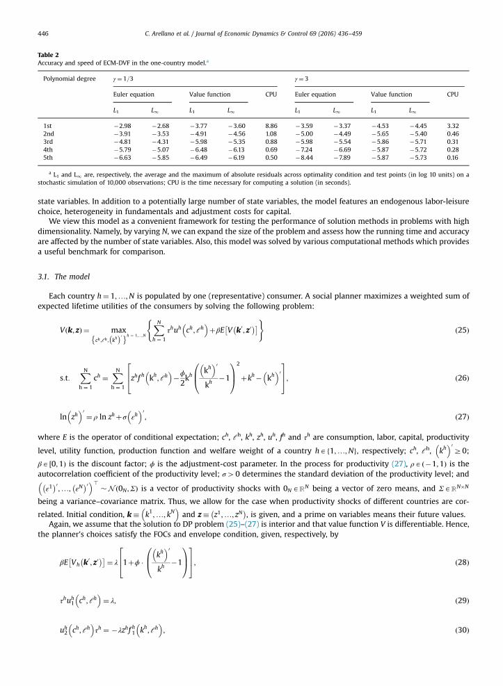
Table 2Accuracy and speed of ECM-DVF in the one-country model.a

Polynomial degree γ ¼ 1=3 γ ¼ 3

Euler equation Value function CPU Euler equation Value function CPU

L1 L1 L1 L1 L1 L1 L1 L1

1st �2.98 �2.68 �3.77 �3.60 8.86 �3.59 �3.37 �4.53 �4.45 3.322nd �3.91 �3.53 �4.91 �4.56 1.08 �5.00 �4.49 �5.65 �5.40 0.463rd �4.81 �4.31 �5.98 �5.35 0.88 �5.98 �5.54 �5.86 �5.71 0.314th �5.79 �5.07 �6.48 �6.13 0.69 �7.24 �6.69 �5.87 �5.72 0.285th �6.63 �5.85 �6.49 �6.19 0.50 �8.44 �7.89 �5.87 �5.73 0.16

a L1 and L1 are, respectively, the average and the maximum of absolute residuals across optimality condition and test points (in log 10 units) on astochastic simulation of 10,000 observations; CPU is the time necessary for computing a solution (in seconds).


state variables. In addition to a potentially large number of state variables, the model features an endogenous labor-leisurechoice, heterogeneity in fundamentals and adjustment costs for capital.

We view this model as a convenient framework for testing the performance of solution methods in problems with highdimensionality. Namely, by varying N, we can expand the size of the problem and assess how the running time and accuracyare affected by the number of state variables. Also, this model was solved by various computational methods which providesa useful benchmark for comparison.

3.1. The model

Each country h¼ 1;…;N is populated by one (representative) consumer. A social planner maximizes a weighted sum ofexpected lifetime utilities of the consumers by solving the following problem:

V k; zð Þ ¼ maxch ;ℓh ; kh

� �0� �h ¼ 1;…;N

XNh ¼ 1

τhuh ch;ℓh

þβE V k0; z0� �� ( )

ð25Þ

s:t:XNh ¼ 1

ch ¼XNh ¼ 1

zhf h kh;ℓh

�ϕ

2kh

kh 0

kh�1

0B@1CA

2

þkh� kh 0

264375; ð26Þ

ln zh 0

¼ ρ ln zhþσ εh 0

; ð27Þ

where E is the operator of conditional expectation; ch, ℓh, kh, zh, uh, fh and τh are consumption, labor, capital, productivity

level, utility function, production function and welfare weight of a country hA 1;…;Nf g, respectively; ch, ℓh, kh 0

Z0;

βA 0;1½ Þ is the discount factor; ϕ is the adjustment-cost parameter. In the process for productivity (27), ρA �1;1ð Þ is theautocorrelation coefficient of the productivity level; σ40 determines the standard deviation of the productivity level; and

ε1� �0

;…; εN� �0 >

�N 0N ;Σð Þ is a vector of productivity shocks with 0NARN being a vector of zero means, and ΣARN�N

being a variance–covariance matrix. Thus, we allow for the case when productivity shocks of different countries are cor-

related. Initial condition, k� k1;…; kN

and z� z1;…; zN� �

, is given, and a prime on variables means their future values.Again, we assume that the solution to DP problem (25)–(27) is interior and that value function V is differentiable. Hence,

the planner's choices satisfy the FOCs and envelope condition, given, respectively, by

βE Vh k0; z0� �� ¼ λ 1þϕ �

kh 0

kh�1

0B@1CA

264375; ð28Þ

τhuh1 ch;ℓh

¼ λ; ð29Þ

uh2 ch;ℓh

τh ¼ �λzhf h1 kh;ℓh

; ð30Þ


Vh k; zð Þ ¼ λ 1þzhf h1 kh;ℓh

þϕ

2

kh 0

kh

0B@1CA

2

�1

0B@1CA

264375; ð31Þ

where λ is the Lagrange multiplier, associated with the economy's resource constraint (26).

3.2. Envelope condition method

In the multicountry case, we implement versions of the ECM methods that perform policy function iteration instead ofvalue function iteration. This is because, operationally, it is easier to solve for value function given policy function than tosolve for policy functions given value function.

We first eliminate λ by combining FOC (28) and envelope condition (31),

1¼ βE Vh k0; z0� ��

Vh k; zð Þπhþzhf h1 kh;ℓh

h ioh

; ð32Þ

where oh and πh are given by

oh � 1þϕkh

0

kh�1

0B@1CA and πh � 1þϕ

2

kh 0

kh

0B@1CA

2

�1

0B@1CA:

Condition (32) relates today's and tomorrow's derivatives of the value function. We next use (32) to parameterize capitalpolicy functions, namely, we premultiply both sides of (32) with kh

0to obtain

kh 0

¼ βE Vh k0; z0� ��

Vh k; zð Þπhþzhf h1 kh;ℓh

h ioh

kh 0

: ð33Þ

The optimal capital policy functions, kh 0

¼ Kh k; zð Þ, h¼ 1;…;N, must satisfy a fixed point property: if we substitute suchfunctions in the right side of (33 ), we must obtain the same functions in the left side. Conditions (33) for h¼ 1;…;N provideus with a way to implement fixed point iteration on capital policy functions. Namely, we guess some policy functionsKh k; zð Þ, h¼ 1;…;N, substitute them in the right side of (33), recompute kh

0in the left side and iterate on these steps until

convergence.Parameterization (33) is analogous to the one used in Maliar et al. (2011) to reparameterize the Euler equations in model

(25)–(27),

kh 0

¼ Eβuh

1 ch� �0

; ℓh� �0

uh1 ch;ℓh� � πh

� �0 þ zh� �0

f h1 kh 0

; ℓh� �0 h

oh

8<:9=; kh 0

: ð34Þ

This kind of representation of Euler equations was originally used in the context of Monte Carlo based solution methods inwhich parameterizing expectation functions in canonical Euler equations do not identify all model's variables: see Den Haan(1990) and Marcet and Lorenzoni (1999) for related examples. The identification of variables is not an issue for solutionmethods like ECM that builds on deterministic integration techniques. However, solving nonlinear systems of equations (32)can be a non-trivial and costly task, especially, when the dimensionality is large. In contrast, fixed point iteration schemeslike (33) and (34) are straightforward to implement; again, only direct calculations are needed.

3.2.1. ECM-VFThe fixed-point problem for the ECM-VF method in the multicountry model is similar to that in the one-country case,

except that we use policy function iteration instead of value function iteration.


Given Kh k; zð Þ, h¼ 1;…;N for each k; zð Þ:(i) Compute kh

0¼ Kh k; zð Þ, h¼ 1;…;N.

(ii) Find c;ℓð Þ satisfying (26), (29) and (30) for each given k; z;k0� �.

(iii) Find V satisfying V k; zð Þ ¼ PNh ¼ 1 τ

huh ch ;ℓh� �þβE V k0 ; z0

� �� .

(iv) Use V to find Vh k; zð Þ and to infer future values Vh k0 ; z0� �

, h¼ 1;…;N.

(v) Compute bkh� �0

¼ βE Vh k;zð Þ½ �Vh k;zð Þ

πh þ zh f h1 kh ;ℓh� ��

oh kh 0

, h¼ 1;…;N.

The optimal policy functions satisfy bkh� �0

¼ kh 0

, h¼ 1;…;N.


In step (ii), we need to compute c;ℓð Þ satisfying (26), (29) and (30) given k; z;k0� �. This requires us to solve a system of

2Nþ1 equations with 2Nþ1 unknowns c;ℓð Þ and λ. This system can be solved with a standard Newton-style numericalsolver but the cost of such a solver may become prohibitive when the dimensionality of the problem increases. Maliar et al.(2011) show a derivative-free iteration-on-allocation solver that can be used in this context and that can be vectorizedfor speed.

3.2.2. ECM-DVFThe fixed-point problem of the ECM-DVF method for the multicountry case also relies on policy function iteration.


Given Kh k; zð Þ, h¼ 1;…;N for each k; zð Þ:(i) Compute kh

0¼ Kh k; zð Þ, h¼ 1;…;N.

(ii) Find c;ℓð Þ satisfying (26), (29) and (30) for each given k; z;k0� �.

(iii) Find Vh k; zð Þ ¼ uh1 ch ;ℓh� �

πhþzhf h1 kh ;ℓh h i

, h¼ 1;…;N.

(iv) Use Vh to infer future values Vh k0 ; z0� �

, h¼ 1;…;N.

(v) Compute bkh� �0

¼ βE Vh k;zð Þ½ �Vh k;zð Þ

πh þ zh f h1 kh ;ℓh� ��

oh kh 0

, h¼ 1;…;N.

The optimal policy functions satisfy bkh� �0

¼ kh 0

, h¼ 1;…;N.

Again, in step (iii), we need to solve the same system of equations as under ECM-VF, i.e., to compute c;ℓð Þ satisfying (26),(29) and (30) given k; z;k0� �

.

3.2.3. Making ECM tractable in high-dimensional problemsThe ECM approaches focus on one specific issue, namely, on how to reduce the computational cost of solving for value

function and its derivatives using the optimality conditions. However, to build a solution method, we need to specify othercomputational choices such as a grid for finding a solution, a function for approximations, an integration method, a fittingmethod, etc. Recent literature distinguished techniques that are tractable in high-dimensional applications in the context ofEuler equation methods; these are non-product grids, low-cost accurate monomial integration rules, derivative-free solvers;see Krueger and Kubler (2004), Malin et al. (2011), Pichler (2011), Maliar et al. (2011), Judd et al. (2011, 2012), and Maliar andMaliar (2015); see also Maliar and Maliar (2014) for a review. The ECM methods are fully compatible with all thesetechniques.

We choose to implement ECM-VF and ECM-DVF following the design of generalized stochastic simulation algorithm(GSSA) method of Judd et al. (2011). GSSA uses a set of points produced by stochastic simulation as a grid for finding asolution. In this sense, it is similar to simulation-based Euler equation and value function iteration methods introduced inMarcet (1988) and Maliar and Maliar (2005), respectively.4 However, GSSA differs from the latter methods in two respects:first, to insure numerical stability, it uses fitting methods that are suitable for dealing with ill-conditioned problems andsecond, to attain high accuracy of solutions, it uses non-stochastic (monomial and quadrature) integration rules. As a result,GSSA delivers accuracy levels that are comparable to the best accuracy attained in the related literature and that areinfeasible for pure simulation methods; see Judd et al. (2011) for a discussion and numerical examples.


We now present the results of numerical experiments for the multicountry model.

3.3.1. Computational choicesWe apply the ECM methods to solve Model II with an asymmetric specification; see the comparison analysis of Kollmann

et al. (2011b). We chose this model among others because it represents all challenges posed in the comparison analysis,namely, a large number of state variables, elastic labor supply, heterogeneity in fundamentals and the absence of closed-form expressions for next-period state and control variables.5 The utility and production functions are given by

uh cht ;ℓht

¼ cht� �1�1=γh

1�1=γh�Bh ℓh

t

� �1þ1=ηh

1þ1=ηh; zf h kht ;ℓ

ht

¼ zhA kht

αℓht

1�α�δkh; ð35Þ

where γh;Bh; ηhn o

are the utility-function parameters; α is the capital share in production; A is the normalizing constant inoutput; δA 0;1ð � is the depreciation rate. We calibrate the model as in Kollmann et al. (2011b). We use the following values of

4 Marcet's (1988) method is developed in Den Haan and Marcet (1990) and Marcet and Lorenzoni (1999).5 Model I has a degenerate labor-leisure choice, and Models III and IV are identical to Model II up to specific assumptions about preferences and

technologies. Juillard and Villemot (2011) provide a description of all models studied in the comparison analysis of Kollmann et al. (2011b).

Table 3Accuracy and speed of ECM-VF in the multicountry model.

Number of countries Polyn. degree CPU r¼0.01 r¼0.1 r¼0.3 Simulation

L1 L1 L1 L1 L1 L1 L1 L1

ECM-VF methodN¼2 2nd 29 �4.95 �3.66 �4.12 �2.69 �3.62 �2.13 �3.97 �2.51

3rd 34 �5.09 �3.71 �4.14 �2.72 �3.65 �2.18 �4.01 �2.51N¼4 2nd 155 �4.90 �3.66 �3.96 �2.70 �3.48 �2.13 �3.86 �2.48

3rd 1402 �4.92 �3.68 �3.99 �2.74 �3.50 �2.20 �3.90 �2.50N¼6 2nd 629 �4.86 �3.64 �3.91 �2.68 �3.43 �2.08 �3.84 �2.47

3rd 21,809 �4.88 �3.66 �3.95 �2.69 �3.47 �2.16 �3.88 �2.51N¼8 2nd 2888 �4.84 �3.62 �3.88 �2.65 �3.40 �2.04 �3.83 �2.48

3rd 89,872 �4.92 �3.68 �3.94 �2.66 �3.41 �1.94 �3.90 �2.48

ECM-DVF methodN¼2 1st 173 �5.14 �4.24 �4.78 �3.14 �4.00 �2.25 �4.82 �3.01

2nd 1189 �6.58 �5.73 �6.22 �4.49 �5.22 �3.14 �6.06 �4.213rd 1734 �7.84 �6.95 �7.37 �5.56 �6.00 �4.08 �7.10 �4.93

N¼4 1st 531 �5.12 �4.32 �4.65 �3.37 �3.84 �2.48 �4.82 �3.192nd 2039 �6.35 �5.61 �6.22 �4.61 �5.14 �3.53 �6.01 �4.323rd 8092 �7.47 �6.52 �6.95 �5.51 �5.65 �3.98 �6.87 �4.89

N¼6 1st 635 �5.10 �4.30 �4.60 �3.36 �3.79 �2.56 �4.83 �3.262nd 2723 �6.71 �5.71 �5.94 �4.48 �4.97 �3.44 �5.88 �4.273rd 38,698 �7.28 �6.37 �6.66 �5.12 �5.25 �3.74 �6.61 �4.76

N¼8 1st 1071 �5.11 �4.29 �4.58 �3.42 �3.76 �2.62 �4.84 �3.342nd 4541 �6.55 �5.65 �5.69 �4.34 �4.74 �3.31 �5.72 �4.163rd 165,911 �7.35 �6.46 �6.42 �4.82 �5.00 �3.40 �6.46 �4.71

Notes: Columns “r¼0.01”, “r¼0.1”, “r¼0.3” contain the results of accuracy evaluation across 1000 draws of state variables located on spheres in the statespace (centered at steady state) with radii 0.01, 0.10, and 0.30, respectively, and column “Simulation” contains the results of accuracy evaluation on astochastic simulation of 10,000 observations. The statistics L1 and L1 are, respectively, average and maximum absolute unit-free residuals (in log 10 units)across all equilibrium conditions. CPU is the running time (in seconds).


common-for-all-countries parameters: α¼ 0:36, β¼ 0:99, δ¼ 0:025, σ ¼ 0:01, ρ¼ 0:95, ϕ¼ 0:5, and we assume that thecountry-specific utility-function parameters γh and ηh are uniformly distributed in the intervals 0:25;1½ � and 0:1;1½ � acrosscountries h¼ 1;…;N, respectively. The steady state level of productivity is normalized to one, zh ¼ 1. We also normalize thesteady state levels of capital and labor to one, k

h ¼ 1, ℓh ¼ 1, which implies ch ¼ A, λ ¼ 1 and leads to A¼ 1�βαβ , τh ¼ uh A;1ð Þ

and Bh ¼ 1�αð ÞA1�1=γh . We consider N¼2, 4, 6 and 8.We parameterize value function (ECM-VF) and the derivative of value function (ECM-DVF) with complete ordinary

polynomials of degrees 2, 3 and 1, 2, 3, respectively. As an initial guess, we use a linear approximation of capital policyfunction. To solve for the polynomial coefficients, we use fixed point iteration. To solve for consumption and labor satisfying(26), (29) and (30), we use an iteration-on-allocation solver developed in Maliar et al. (2011). To approximate integrals, weuse a monomial integration rule M1 with 2N nodes, and to fit the value and policy functions to simulated data, we use aleast-squares truncated QR factorization method; see Judd et al. (2011) for a description of these techniques. We use thesame software and hardware as that used to solve the one-country model. We provide a detailed description of the studiedECM methods in Appendix B.

3.3.2. ResultsIn Table 3, we present the results produced by two versions of the ECM method, ECM-VF that solves for value function

and ECM-DVF that solves for derivative of value function. We report two accuracy measures: one measure is the size ofabsolute unit-free residuals across 1000 draws of state variables located on spheres in the state space (centered at steadystate) with radii 0.01, 0.10, and 0.30. Roughly speaking, this measure shows how accurate our solution is when we deviatefrom the steady state by 1%, 10% and 30%, respectively. The other measure is the size of the residuals on a stochasticsimulation of 10,000 observations; this measure shows how accurate our solution in the high-probability area of the statespace – the ergodic set. These two accuracy measures are used in the JEDC comparison analysis of Kollmann et al. (2011b);also see Juillard and Villemot (2011) for more details.

Our main finding is that the ECM methods are tractable in the context of the given multidimensional problem. Moreover,the ECM methods are able to produce not only the second-degree but also far more expensive third-degree polynomialapproximations. All Euler equation methods studied in Kollmann et al. (2011b) are limited to second-degree polynomialapproximation. The ECM methods have an advantage over Euler equation methods in that they solve for control variablesonly at present and do not need to find such variables in all integration nodes. This advantage can be especially important inhigh-dimensional problems as the number of integration nodes grows rapidly with dimensionality.

As far as the accuracy is concerned, ECM-VF is considerably less accurate than ECM-DVF. Our results suggest that in high-dimensional problems, approximating value function with polynomial on a grid does not produce accurate approximations


for derivatives of value function. This is the same effect that we observed in Section 2.5.1 for the one-agent model, namely, ifwe approximate V with polynomial, we effectively approximate V1 with polynomial of one degree less, i.e., we “lose” onepolynomial degree.

In turn, the ECM-DVF method is very accurate. It reaches the accuracy frontier attained in the comparison analysis ofKollmann et al. (2011b). In particular, in an accuracy check on a stochastic simulation, our third-degree polynomial solutionsare more accurate than second-degree polynomial solutions reported in Kollmann et al. (2011b) although our second-degreepolynomial solutions are somewhat less accurate than their most-accurate solutions. For example, for a model with N¼8countries, the second- and third-degree ECM-DVF polynomial solutions have maximum residuals across the optimalityconditions of orders 10�4:16 and 10�4:71, respectively. For comparison, the most accurate second-degree method in Koll-mann et al. (2011b) produces maximum residual of order 10�4:50. Thus, we conclude that ECM value iteration methods cansuccessfully compete with the state-of-the-art Euler equation methods.6

4. ECM for default risk models

Default risk models focus on borrowing-lending arrangements in which debt is unsecured and a borrower can default ondebt. Examples of situations with default include sovereign default (e.g, Greek default of 2012; Argentinian default of 2001),consumer bankruptcy (defaults on loans and mortgages), firm bankruptcy (defaults on financial or contractual obligations),local government defaults (e.g., Detroit in 2013), etc.

The recent financial and sovereign debt crises worldwide has sparked a growing literature on quantitative models ofdefaultable debt. Arellano (2008) studied quantitatively the implications of the seminal paper of Eaton and Gersovitz (1981)and showed that it was useful for understanding sovereign default in emerging markets. Aguiar and Gopinath (2006)showed the importance of shocks to trend for output in emerging economies in the context of a sovereign default model.Chatterjee et al. (2007) provided a framework to study consumer bankruptcy in the United States. Their model can ratio-nalize the cross section distribution of bankruptcies across households of different characteristics. Maliar et al. (2008)constructed a default risk model of FDI and capital controls; they argue that scarce capital flow from rich to poor nations canbe explained by a risk of expropriation. Hopenhayn and Werning (2008) analyzed the optimal financing of an investmentproject subject to the risk of default and show that the optimal contract may allow default along the equilibrium path.Arellano et al. (2013) studied the implications of firm default for business cycles and for the Great Recession in the UnitedStates. Tsyrennikov (2013) analyzed optimal fiscal and default policy in default risk models. Bianchi et al. (2009) used adefault risk model for investigating the optimal accumulation of international reserves as a hedge against roll over risk.Aguiar et al. (2015) studied fiscal and monetary policy in a monetary union with the potential for rollover crises in sovereigndebt markets. See Aguiar and Amador (2013) for a review of the literature on sovereign debt. The main challenge for thisliterature, however, is the computational burden of models with default. Computational limitations constitute a substantialobstacle to analyze richer models. We argue that the ECM methods can significantly reduce the computational expense ofdefault risk models.

4.1. A default risk model

We study a variant of the default risk model of Arellano (2008). A country-borrower may decide to default when the debtis getting too large and or when facing a large negative shock.

A borrower's problem: A country-borrower is populated by a representative household with preferences E0P1

t ¼ 0 βtu ctð Þ

where u is strictly increasing, continuously differentiable and concave and βA 0;1ð Þ. The borrower receives exogenousstochastic income yt which follows an AR1 process

logðytÞ ¼ ρlogðyt�1Þþεt ; ð36Þ

with εt �N 0; σ2� �

, ρA �1;1ð Þ, and σZ0.The borrower trades one period bonds with international lenders and can default on the bonds. When the borrower has

bonds bt ; income yt ; and does not default, it can choose new bond btþ1 at price qðbtþ1; ytÞ: Consumption in this case is

ct ¼ ytþbt�qðbtþ1; ytÞbtþ1:

A negative value of b means that the country issues bonds to borrow; qðbtþ1; ytÞ is the price that a borrower will pay for aunit bond depending on the quantity of bonds issued by the country btþ1 and its current state yt. These variables determinethe probability of default in the next period. The borrower takes as given the bond price function.

6 The only method (apart from ECM) that has produced third-degree polynomial solutions to a similar model is a perturbation-based hybrid Eulerequation method of Maliar et al. (2013). This method computes some policy functions locally (using perturbation) and computes the remaining policyfunctions globally (using analytical formulas and numerical solvers). In the given model with N¼8 countries, this method delivers maximum residuals oforder 10�4:69.


Default decision: The borrower can default at any time on the debt bt it owes and pay 0. If a borrower defaults, he goes toautarky and gets punished with reduced output ydry in every period spent in autarky. In the future, the borrower re-incorporates in the world economy with exogenously given probability θ.

Lenders' problem and bond-price function: Lenders are risk neutral and perfectly competitive. Their problem is

maxbt þ 1

qtbtþ1�1�δt1þr

btþ1

� �; ð37Þ

where r is a risk-free interest rate, and δt is a probability of a borrower to default. A zero-profit condition implies thatqt ¼ 1� δt

1þ r . If δt ¼ 0 (i.e., a borrower never defaults), then qt ¼ 11þ r (risk-free interest rate), and if δt ¼ 1 (i.e., a borrower always

defaults), then qt ¼ 0 (bonds are worthless). If a borrower defaults with some probability δtA 0;1ð Þ, then we haveqtA 0; 1

1þ r

.

A recursive formulation of Arellano's (2008) model: To formulate a Bellman equation for the consumer's problem, weintroduce two value functions Vd yð Þ and Vðb; yÞ that correspond to default and no-default states. To decide whether todefault or not, an agent compares these two possibilities and chooses the one that implies higher welfare,

Voðb; yÞ � max Vðb; yÞ;Vd yð Þn o

: ð38Þ

However, by assumption the borrower chooses default if Vðb; yÞoVðb; y bð ÞÞ � Vd yð Þ. If a borrower does not default, his valuefunction V satisfies

Vðb; yÞ ¼maxb0

uðcÞþβ

Zmax Vðb0; y0Þ;Vðb0; y b0

� �Þ� �dFðy0Þ

� �s:t: c¼ yþb�q b0; y

� �b0; ð39Þ

where F is a distribution function of y0 and q b0; y� �

is the bond-price function that is related to the probability of defaultδ b0; y� �

as q b0; y� �¼ 1� δ b0 ;yð Þ

1þ r . If a borrower defaults, his value function Vd is given by

Vd yð Þ ¼ u yd

þβE θVoð0; y0Þþ 1�θð ÞVd y0ð Þh i

; ð40Þ

where θ is the probability of re-incorporating in the world economy after default, and ydry is a direct output cost fromdefaulting. By changing θ and yd, we can affect Vd yð Þ and hence, the borrower's incentives to default.

A version of the default risk model with an exogenous default rule: We will also consider a version of default risk model withexogenous default risk rule. Namely, we assume that the borrower's default decision is represented by an exogenousfunction y btð Þ such that an agent with the debt bt will default whenever the random income yt falls below the thresholdlevel ytoy btð Þ. By using (36), we can compute the probability of default δ btþ1; yt

� �at tþ1

δ btþ1; yt� �¼ prob yρt exp εtð Þ|fflfflfflfflfflffl{zfflfflfflfflfflffl}

ytþ 1

oy btþ1ð Þ

0B@1CA¼ F ln

y btþ1ð Þyρt

� �� ; ð41Þ

where F is a cumulative distribution function of a normal distribution. Using (41), we can represent the price functionq btþ1; yt� �

by

q btþ1; yt� �¼ 1

1þr1�F ln

y btþ1ð Þyρt

� �� : ð42Þ

The probability of default q btþ1; yt� �

increases with the amount of debt btþ1, and it decreases with income yt.Endogenous versus exogenous default rule: There is a relation between Arellano (2008) model and the default risk model

with exogenous default rule. In the model of Arellano (2008), a condition for default is defined implicitly by (38): a borrowerdefaults for those y for which Vðb; yÞoVd yð Þ given b. For the case of i.i.d. shocks and when the cost of default is limited toexclusion from the borrowing market, Arellano (2008) showed that the default decision is a cutoff rule of type y bð Þ. Inquantitative simulations for more general shock processes and default costs, that paper also contains default decisions thatare cutoff rules. Hence, the cutoff rule for default y bð Þ induces the corresponding value function condition Vðb; yÞoVd yð Þ andvice versa. In particular, if we take the cutoff rule y bð Þ that is implied by Arellano (2008) analysis, we will get the samesolution in the models with endogenous and exogenous default rules.

Thus, the model with exogenous default rule is useful for three reasons: first, the ECM analysis requires us to solve such amodel as a part of the solution procedure of Arellano (2008) model with endogenous default rule. Second, the model withexogenous default rule is a convenient setup for testing the performance of the proposed numerical solution methods.Finally, the model with exogenous default rule has interest of its own and can be used as a simpler alternative to theconventional model with endogenous default rule in some applications.

Fig. 1. Discretization method: value function, policy functions and prices.


4.2. Envelope condition method

Assuming differentiability of the price and value functions, in those states in which default does not occur yZy bð Þ, thequantity of issued bonds b0 satisfies the following FOC:

u0ðcÞ½q1ðb0; yÞb0 þqðb0; yÞ� ¼ βE Vo1ðb0; y0Þ

� �: ð43Þ

The envelope condition, V1ðb; yÞ ¼ u0ðcÞ, in turn implies the following ECM-DVF recursion

V1 b; yð Þ ¼ βE Vo1ðb0; y0Þ

� �q1ðb0; yÞb0 þqðb0; yÞ ¼

βRV1ðb0; y0Þ1 y04y b0

� �� dFðy0Þ

q1ðb0; yÞb0 þqðb0; yÞ ; ð44Þ

where 1ðXÞ is an indicator of the event X, and F is a distribution function of y0. The term corresponding to the indicatorfunction 1ðy0ry b0

� �Þ does not appears in (44) because for y0ry b0� �

, we have Vo1 b0; y0� �¼ ∂Vd y0ð Þ

∂b0 ¼ 0. Although value functionhas a kink in the default point, it is never optimal for the agent to reach that point (this fact follows by the generalizedenvelope theorem of Clausen and Strub, 2013). As a result, the optimal choice satisfies (43) and (44).

4.2.1. ECM-VF for the model with an exogenous default ruleWe first show ECM-VF for the default risk model with exogenous default rule (39), (40) and (42).

Fix y bð Þ and choose a set of points b; yð Þ such that y4y bð Þ.Precompute qðb0 ; yÞ using (42).Define ðb0 ; yÞ � qðb0 ; yÞb and precompute its inverse �1.Given Vðb; yÞ, for each point b; yð Þ, compute:
(i). c¼ u0�1 V1ðb; yÞ� �

.

(ii). b0 ¼ �1ðbþy�cÞ.(iii). bV ðb; yÞ ¼ u cð ÞþβE max Vðb0 ; y0Þ;Vðb0 ; y b0

� �Þ� �� .


While we can solve for b0 satisfying (39) for each point b; yð Þ within the main iterative cycle, doing so would be costlybecause we need to use a nonlinear solver a large number of times. Precomputation – constructing a part of a numericalsolution outside the main iterative cycle – can speed up computation greatly; see Maliar and Maliar (2014) for review ofprecomputation techniques for dynamic economic models.

4.2.2. ECM-DVF for the model with an exogenous default ruleWe now show ECM-DVF for the default risk model with an exogenous default rule (39), (40) and (42).


Fix y bð Þ and choose a set of points b; yð Þ such that y4y bð Þ.Precompute qðb0 ; yÞ using (42).Define ðbÞ � qðbÞb and precompute its inverse �1.Given V1ðb; yÞ, for each point b; yð Þ, define:
(i) c¼ u0�1 V1ðb; yÞ� �

.

(ii) b0 ¼ �1ðbþy�cÞ.(iii) bV 1 b; yð Þ ¼ βE Vo

1 ðb0 ;y0 Þ½ �q1 ðb0 ;yÞb0 þqðb0 ;yÞ ¼

βR

V1 ðb0 ;y0 Þ1 y0 4y b0ð Þð ÞdFðy0 Þq1 ðb0 ;yÞb0 þqðb0 ;yÞ .

The optimal value function satisfies bV 1 ¼ V1.

Given a converged bV 1, find bV satisfying bV ðb; yÞ ¼ u cð ÞþβE max bV ðb0 ; y0Þ; bV ðb0 ; y b0� �Þn oh i

.

When implementing ECM-DVF, one needs to be careful not to include grid points for which q1ðb0; yÞb0 þqðb0; yÞo0. As wasshown in Arellano (2008), the amount of resources that a country can borrow follows a Laffer curve. Initially, the loanðbÞ � qðbÞb decreases with b, then it reaches its maximum and finally, it decreases to zero because an increased risk of defaultquickly drives the bond price q(b) to zero which dominates the product qðbÞb; see Fig. 1 for an example of the Laffer curve. Aborrower can never be on a negatively sloped portion of that Laffer curve.

4.2.3. ECM for the model with an endogenous default ruleAn algorithm for solving the version of the model (38)–(40) with endogenous default risk is identical to the one used in

Arellano (2008) except that the conventional VFI iteration cycle is replaced by ECM-VF and ECM-DVF methods.To be more specific, given Vðb; yÞ and Vd yð Þ, we first find the cut-off rule y bð Þ satisfying Vðb; yÞ ¼ Vd yð Þ (according to (38),

the agent will default whenever yoy bð Þ). Next, for given exogenous default rule yoy bð Þ, we solve for the new valuefunction bV using either Algorithm 10 or Algorithm 11, and we update the autarky value function Vd according to (40). If Vand Vd converged, we end iteration; otherwise, we proceed to next iteration.


We now construct numerical solutions for the default risk model. We first report the results for the test model with anexogenous default rule, and we then study Arellano (2008) model with an endogenous default rule.

4.3.1. The model with an exogenous default ruleAs an example, we consider a simple default rule ytryðbtÞ � n�bt , where n is an exogenous lower bound on the bor-

rower's net worth. The borrower with the mean income level yt ¼ 1 would default when its debt rises above 1�n. Weconsider three values of n ¼ 0:65;0:75;0:95f g that imply that the borrower's debt rises above 0.35, 0.25 and 0.05 of anaverage period's income, respectively. We assume that the income in (36) is i.i.d, y�N ð0;0:05Þ. Then, the probability ofdefault (41) is given by

δ btþ1; yt� �¼ probðytþ1ryðbtþ1ÞÞ ¼ Fðn�btþ1Þ;

where F is a distribution function of a Normal distribution. We choose the remaining parameters in line with Arellano(2008), namely, we parameterize the utility function by u cð Þ ¼ c1� γ �1

1� γ with γ ¼ 2, and we fix β¼ 0:94.We solve the model on bA ½�0:18;0:40�. For each realization of output y we approximate the unknown value function

and its derivative using a cubic spline with 21 nodes. Grid points are Chebyshev extrema scaled so that b1 ¼ �0:18,b100 ¼ 0:40. (As an alternative, we tried to use grid points that are uniformly spaced and we find that it leads to comparableand slightly lower accuracy measures). To perform integration with respect to y0, we use a Gauss–Hermite quadrature rulewith 11 nodes. We implemented three algorithms: ECM-VF, ECM-DVF and conventional VFI which construct policy functionsusing FOC. We find that ECM-VF is less stable numerically in the default risk model and requires a sufficiently accurate initialguess for convergence, while ECM-DVF is more robust to the choice of an initial guess. For all the three algorithms, we usean identical convergence criterion that the (maximum across nodes) change in the value function was smaller than 10�4. All

Table 4Accuracy and speed of ECM-VF and ECM-DVF in the one-country model.a

Default rule ECM-VF ECM-DVF VFI

L1 L1 CPU L1 L1 CPU L1 L1 CPU

yðbÞ ¼ 0:65�b �3.85 �3.32 5.41 �3.00 �2.92 5.32 �3.85 �2.83 412.24yðbÞ ¼ 0:75�b �3.86 �3.34 5.48 �3.00 �2.92 5.34 �3.86 �3.34 282.24yðbÞ ¼ 0:95�b �3.85 �3.40 5.39 �2.99 �2.93 5.29 �3.48 �3.00 295.13

a L1 and L1 are, respectively, the average and the maximum of unit-free absolute residuals in Bellman equation across test points (in log 10 units) on astochastic simulation of 10,000 observations; CPU is the time necessary for computing a solution (in seconds).

Fig. 2. Envelope condition method: value function, policy functions and prices.


calculations are performed in MATLAB 2013b on a laptop with an 2.9 GHz Intel i7-3520 M processor. We provide a detaileddescription of the studied computational methods in Appendix C.

In Table 4, we report the running time and accuracy measures on a stochastic simulation produced by ECM-VF and ECM-DVF, and we compare the results with those produced by a conventional VFI. The standard VFI takes about 282.2 s toconverge, while the ECM-VF and ECM-DVF methods take both about 5.5 s; hence, we observe about 50� speedups orhigher. As in all previous numerical experiments, the accuracy of ECM-VF is somewhat lower than that of ECM-DVF as was inall the previous experiments.

4.3.2. The model with endogenous default ruleWe next apply ECM for solving Arellano (2008) model with an endogenous default rule. In such a model, the con-

vergence of ECM was more difficult to attain. Specifically, a simultaneous iteration on both value functions and endogenousbond price function led to numerical errors that accumulate along iterations, resulting in non-monotone policy functions.Significant damping was needed to stabilize explosive iteration.

We find that the best use of the ECM method in the context of the given problem is to refine a low accuracy solutionproduced by a version of VFI based on discretization. To be specific, we discretize the domain for bonds into 1000 equallyspaced grid points b1;…; b1000, where b1 ¼ �0:18 and b1000 ¼ 0:40, and we solve for value function by finding maximum ofthe right side of Bellman equation (39) across a finite number of discretized bond holdings. The running time was low, 22 s,but the accuracy of the solution was also low.

We show the constructed value function, policy functions and prices produced by the conventional VFI discretizationmethod in Fig. 1.

As is seen from Fig. 1, the constructed value and decision functions have the form of step functions. This indicates thatthe discretization method produces considerable approximation errors. Indeed, the average and maximum unit-free resi-duals in the Bellman equation on a solution domain (39) are �1.84 and �0.84, respectively, indicating that the approx-imation errors can be as large as 15% for the VFI method based on discretization.

We next refine the VFI solution using ECM-VF implemented on the same 1000 grid points. The running time for the ECMmethod was approximately 8 seconds. In Fig. 2, we plot the constructed value function, policy functions and prices of theECM solution.

The step functions are not appreciated for the ECM solution. This is because the constricted policy and value functions areaccurately interpolated off the grid points using cubic splines. The average and maximum unit-free residuals in the Bellmanequation on a solution domain (39) are �4.85 and �3.09 after the refinement, respectively. This indicates that the residualsare of order 0.1%, which is about 100 times smaller than those produced by the VFI discretization method. It would bepossible to attain higher accuracy levels under conventional VFI if a finer grid is used, for example, 100,000 points instead of1000 points but memory of our computer was insufficient to run such experiments. In contrast, ECM was feasible andrequired just few seconds to produce highly accurate solution.


5. Conclusion

In the paper, we focus on a broad and empirically relevant class of DP problems characterized by a large, finite number ofcontinuous state variables and a differentiable value function. There are three main challenges that such problems representto numerical solution methods. First, the number of arguments in value and policy functions increases with the dimen-sionality of the problem and such functions become costly to approximate numerically. Second, the cost of integrationincreases as the number of exogenous random variables increases. Finally, larger problems are normally characterized bylarger and more complex systems of equations which are more expensive to solve. Moreover, some applications requiresolving a sequence of similar economic models a large number of times, for example, nested fixed point methods foreconometric estimation as in Fernández-Villaverde and Rubio-Ramírez (2007) and extended function path (EFP) frameworkof Maliar et al. (2015) for analyzing nonstationary and unbalanced growth models.

We develop ECM methods for DP problems that are aimed to address these challenges. Concerning the first two chal-lenges, we build ECM on non-product approximation, integration and interpolation techniques that are designed for dealingwith high-dimensional problems; see Maliar and Maliar (2014) for a review of such techniques. The last challenge is themain focus of our analysis, namely, we replace conventional expensive VFI based on FOCs or direct maximization with acheap forward-style ECM iteration based on the envelope condition. We show that the computational expense of high-dimensional applications can be reduced even further by combining value and policy function iteration.

We find that solving for value function does not accurately identify the derivatives of value function. The accuracy of ECMcan be significantly increased by solving for the derivatives of value function instead of the value function itself, or, alter-natively, by solving jointly for value function and its derivatives. In the context of large-scale models studied in the JEDCproject, the version of the ECM method that approximates derivatives of value function can successfully compete with thestate-of-the-art Euler equation methods. Moreover, the ECM methods produce accurate solutions to challenging default riskmodels with a kink in value and policy functions and is faster by orders of magnitude than conventional VFI in our exampleswith exogenous default rules. These are promising results given a high computational expense of default risk models.However, the convergence of ECM methods was hard to achieve in a default risk model with endogenous default rules.Further research is needed to enhance the convergence properties of the ECM methods in this class of models.

Acknowledgments

We are indebted to Editor Chris Otrok and two very competent anonymous referees for many thoughtful comments andsuggestions. Also, we benefited from comments of Francisco Buera, Jesús Fernández-Villaverde, Grace Gu, Kenneth L. Judd,Seung Lee, Marcelo Veracierto, Mark Wright, seminar participants at Bank of Canada, Boston University, Federal ReserveBank of Chicago, Indiana University, Santa Clara University, Stanford University, University of California at Santa Cruz as wellas from participants of the 2014 meeting of Society of Computational Economics and the 2015 meetings of Society forEconomic Dynamics and Econometric Society. Errors are ours. Support from the Hoover Institution and Department ofEconomics at Stanford University, University of Alicante, Santa Clara University and the MINECO/FEDER grant ECO2015-70540-P is gratefully acknowledged.

Appendix

In Appendix A, we provide a description of ECM-VF and ECM-DVF for the one-country model. In Appendix B, we describehow to implement these methods for the multicountry model. Finally, in Appendix C, we show numerical methods used tosolve a default risk model.

Appendix A. ECM for the one-agent model

We first describe the ECM-VF method that solves for value function in one-agent model (1)–(3).

Algorithm 1. ECM-VF (with implementation details).
Initialization.
(i) Choose an approximating function V �; að Þ V .(ii) Choose integration nodes, εj, and weights, ωj, j¼ 1;…; J.(iii) Construct a grid km ; zm

� �m ¼ 1;…;M .

(iv) Make an initial guess on a 1ð Þ .

Iterative cycle. At iteration n, given a nð Þ , perform the following steps.


Step 1. For m¼ 1;…;M, compute:

(i) cm ¼ V1 km ;zm ;a nð Þð Þ1� δþ zαkα� 1

m

� ��1=γ

.

(ii) k0m ¼ 1�δð Þkmþzmkαm�cm .

(iii) vm ¼ c1� γm �11� γ þβ

PJj ¼ 1 ωjV k0m ; z

ρmexp εj

� �; a nð Þ� �

.

Step 2. Computation of a that fits the values vm on the grid.

Run a regression to find ba ¼ argmina

PMm ¼ 1 vm�V km ; zm; að Þ

�� .Step 3. Convergence check and fixed-point iteration.

Stop if 1ξM

PMm ¼ 1

k0mð Þ nþ 1ð Þ � k0mð Þ nð Þ

k0mð Þ nð Þ

o10�10, where ξ¼ 0:1 is a damping parameter.

Otherwise, use damping to compute a nþ1ð Þ ¼ 1�ξð Þa nð Þ þξba and go to Step 1.

We next describe ECM-DVF that solves for the derivatives of value function in the one-country model (the steps that areidentical to those in ECM-VF are omitted).

Algorithm 6. ECM-DVF (with implementation details).
Initialization.
(i) Choose an approximating function V1 �; að Þ V1.…

Iterative cycle. At iteration n, given a nð Þ , perform the following steps.

Step 1. For m¼ 1;…;M, compute…

(iii) dm ¼ β 1�δþαzkα�1m

h iPJj ¼ 1 ωjV1 k0m ; z

ρmexp εj

� �; a nð Þ� �

.

Step 2. Computation of a that fits the values dm on the grid.


PMm ¼ 1 dm�V1 km; zm; að Þ

�� .…

Appendix B. ECM for multicountry model

We now describe the ECM-VF method that solves for value function in multicountry model (25)–(27).

Initialization.
(i) Choose approximating functions Kh �; ah� � Kh , h¼ 1;…;N and V �;ϖð Þ V .

(ii) Choose integration nodes, εj ¼ ε1j ;…; εNj

, and weights, ωj, j¼ 1;…; J.

(iii) Fix the simulations length T and the initial condition k0 ; z0ð Þ.(iv) Draw and fix a sequence of productivity levels ztf gt ¼ 1;…;T using (27).

(v) Construct integration nodes, ztþ1;j ¼ zhtþ1;j;…; zhtþ1;j

with zhtþ1;j ¼ zht

� �ρexp εhj

.

(vi) Make an initial guess on a1� � 1ð Þ

;…; ah� � 1ð Þ

.

Iterative cycle. At iterationn, given a1� � nð Þ

;…; ah� � nð Þ

, perform the following steps.

Step 1. For t ¼ 1;…; T ,

(i) Use khtþ1 ¼ bKhkt ; zt ; ah

� � nð Þ , h¼ 1;…;N, to recursively calculate ktþ1

� �t ¼ 0;…;T .

(ii) Compute ct ;ℓtf gt ¼ 0;…;T satisfying (26), (29) and (30) given kt ; zt ;ktþ1� �

t ¼ 0;…;T .

(iii) Find bϖ satisfying V kt ; zt ; bϖð Þ ¼ PNh ¼ 1 τ

huh cht ;ℓht

� �þβPJ

j ¼ 1 V ktþ1 ; ztþ1;j; bϖ� �.

(iv) Use V �; bϖð Þ to find Vh kt ; zt ; bϖð Þ and to infer Vh ktþ1 ; ztþ1;j; bϖ� �for j¼ 1;…; J.

(v) Compute bkh

tþ1 �PJ

j ¼ 1 βVh kt þ 1 ;zt þ 1;j ;bϖ� �

Vh kt ;zt ;bϖ� � πht þ zht fh1 kht ;ℓ

ht

� �� oht

khtþ1, h¼ 1;…;N.

Step 2. Computation ofah that fits the values bkh

tþ1 on the grid.

Run regressions to find bah � argminah

PTt ¼ 1

bkh

tþ1�Kh kt ; zt ; ah� �� :

Step 3. Convergence check and fixed-point iteration..


Stop if 1TNξ

PTt ¼ 1

PNh ¼ 1

bkh

t þ 1

nþ 1ð Þ� kht þ 1

� � nð Þ

kht þ 1

� � nð Þ

o10�7, where ξ¼ 0:05 is damping parameter.

Otherwise, use damping to compute ah� � nþ1ð Þ ¼ 1�ξð Þ ah

� � nð Þ þξbah and go to Step 1.

We next describe ECM-DVF that solves for the derivatives of value function in the multicountry model (the steps that areidentical to those in ECM-VF are omitted).

Initialization.
(i) Choose approximating functions Kh �; ah� � Kh and Vh �;ϖh� � Vh, h¼ 1;…;N.

…

Iterative cycle. At iterationn, given a1� � nð Þ

;…; ah� � nð Þ

, perform the following steps.

Step 1. For t ¼ 1;…; T ,…

(iii) Find dht � uh1 cht ;ℓ

ht

� �πht þzht f

h1 kht ;ℓ

ht

h iand find bϖh � argmin

ϖhdht �Vh kt ; zt ;ϖh

� �� , h¼ 1;…;N;

(iv) Use Vh U ; bϖh

to find Vh kt ; zt ; bϖh

and to infer Vh ktþ1 ; ztþ1;j; bϖh

for j¼ 1;…; J;

…

Appendix C. ECM for default risk model

We show the ECM-VF method that solves for value function in default risk model (38)–(39).

Initialization.
(i) Choose an approximating function V �; að Þ V .(ii) Choose integration nodes, εj, and weights, ωj, j¼ 1;…; J.(iii) Construct a grid bm; ym

� �m ¼ 1;…;M covering the area y4y bð Þ.

(iv) Compute qðb0 ; yÞ using (42).(v) Define ðbÞ � qðbÞb and precompute its inverse �1.(vi) Make an initial guess on a 1ð Þ .

Iterative cycle. At iterationn, given a nð Þ , perform the following steps.

Step 1. For m¼ 1;…;M, compute:

(i) cm ¼ V1 bm ; zm; a nð Þ� ��1=γ .

(ii) b0m ¼ �1ðbmþym�cmÞ.(iii) vm ¼ c1� γ

m �11� γ þβ

PJj ¼ 1 ωjmax V b0m ; y

ρmexp εj

� �; a nð Þ� �

V b0m ; y bmð Þ; a nð Þ� �� Step 2. Computation ofa that fits the valuesvm on the grid.


PMm ¼ 1 vm�V km ; zm; að Þ

�� .Step 3. Convergence check and fixed-point iteration.

Stop if max v nþ1ð Þm �v nð Þ

m

o10�4, where ξ¼ 0:1 is a damping parameter.

Otherwise, use damping to compute a nþ1ð Þ ¼ 1�ξð Þa nð Þ þξba and go to Step 1.

We next describe ECM-DVF that solves for the derivatives of value function in default risk model (38)–(39) (the steps thatare identical to those in ECM-VF are omitted).

Initialization.
(i) Choose an approximating function V1 �; að Þ V1.…

Iterative cycle. At iterationn, given a nð Þ , perform the following steps.


Step 1. For m¼ 1;…;M, compute…

(iii) dm ¼ βPJ

j ¼ 1ωjV1 b0m ;yρm exp εjð Þ;a nð Þð Þ1 yρmexp εjð Þ4y b0mð Þð Þ

q1 ðb0m ;ym Þb0m þqðb0m ;ym Þ .

…Step 2. Computation of a that fits the values dm on the grid.


PMm ¼ 1 dm�V1 km; zm; að Þ

�� .…

We next describe conventional VFI that solves for value function in default risk model (38)–(39) (the steps that areidentical to those in ECM-VF are omitted).

Algorithm 12. FOC-VFI (with implementation details).
…
Step 1. For m¼ 1;…;M, use a numerical solver to find

(i) maxb0m

c1� γm �11� γ þβ

PJj ¼ 1 ωj max V b0m; y

ρm exp εj

� �; a nð Þ� �

;V b0m ; y bmð Þ; a nð Þ� �� n o,

where cm ¼ bmþym�b0mqðb0m ; ymÞ.…

References

Achdou, Y., Han, I., Lasry, J.M., Lions, P.L., Moll, B., 2015. Heterogeneous Agent Models in Continuous Time. Manuscript.Aguiar, M., Gopinath, G., 2006. Defaultable debt, interest rates and the current account. J. Int. Econ. 69 (1), 64–83.Aguiar, M., Amador, M., 2013. Sovereign Debt: A Review. NBER Working Papers 19388.Aguiar, M., Amador, M., Farhi, E., Gopinath, G., 2015. Coordination and Crisis in Monetary Unions. Manuscript.Arellano, C., 2008. Default risk and income fluctuations in emerging economies. Am. Econ. Rev. 98 (3), 690–712.Arellano, C., Bai, Y., Kehoe, P., 2013. Financial Frictions and Fluctuations in Volatility. Federal Reserve Bank of Minneapolis Staff Report 466.Aruoba, S., Schorfheide, F., 2013. Macroeconomic Dynamics Near ZLB: A Tale of Two Equilibria. NBER Working Paper 19248.Aruoba, S., Fernández-Villaverde, J., Rubio-Ramírez, J., 2006. Comparing solution methods for dynamic equilibrium economies. J. Econ. Dyn. Control 30,

2477–2508.Barillas, F., Fernandez-Villaverde, J., 2007. A generalization of the endogenous grid method. J. Econ. Dyn. Control 31, 2698–2712.Bellman, R., 1957. Dynamic Programming. Princeton University Press, Princeton, NJ.Bertsekas, D.P., Tsitsiklis, J.N., 1996. Neuro-Dynamic Programming. Athena Scientific, Belmont, MA.Bianchi, J., Hatchondo, J.C., Martinez, L., 2009. International Reserves and Rollover Risk. Manuscript.Blackwell, D., 1965. Discounted dynamic programming. Ann. Math. Stat. 36, 226–235.Carroll, K., 2005. The method of endogenous grid points for solving dynamic stochastic optimal problems. Econ. Lett. 91, 312–320.Chatterjee, S., Eyigundor, B., 2011. A Quantitative Analysis of the U.S. Housing and Mortgage Markets and the Foreclosure Crisis. Working Papers 11-26,

Federal Reserve Bank of Philadelphia.Chatterjee, S., Corbae, D., Nakajima, Ríos-Rull, J.V., 2007. A quantitative theory of unsecured consumer credit with risk of default. Econometrica 75

(November), 1525–1589.Clausen, A., Strub, C., 2013. A General and Intuitive Envelope Theorem. Manuscript.Den Haan, W., 1990. The optimal inflation path in a Sidrauski-type model with uncertainty. J. Monet. Econ. 25, 389–409.Den Haan, W., Marcet, A., 1990. Solving the stochastic growth model by parameterized expectations. J. Bus. Econ. Stat. 8, 31–34.Den Haan, W., Judd, K.L., Juillard, M., 2011. Computational suite of models with heterogeneous agents II: multicountry real business cycle models. J. Econ.

Dyn. Control 35, 175–177.Eaton, J., Gersovitz, M., 1981. Debt with potential repudiation: theoretical and empirical analysis. Rev. Econ. Stud. 48 (2), 289–309.Fella, G., 2014. A generalized endogenous grid method for non-smooth and non-concave problems. Rev. Econ. Dyn. 17/2, 329–344.Feng, Z., Miao, J., Peralta-Alva, A., Santos, M., 2009. Numerical Simulation of Nonoptimal Dynamic Equilibrium Models. Working Papers Federal Reserve

Bank of St. Louis 018.Fernández-Villaverde, J., Rubio-Ramírez, J., 2007. Estimating macroeconomic models: a likelihood approach. Rev. Econ. Stud. 74, 1059–1087.Fernández-Villaverde, J., Gordon, G., Guerrón-Quintana, P., Rubio-Ramírez, J., 2012. Nonlinear Adventures at the Zero Lower Bound. NBER Working Paper

18058.Fukushima, K., Waki, Y., 2011. A Polyhedral Approximation Approach to Concave Numerical Dynamic Programming. Manuscript.Gust, C., López-Salido, D., Smith, M., 2012. The empirical implications of the interest-rate lower bound. Federal Reserve Board, Finance and Economics

Discussion Series, No. 2012-83.Hasanhodzic, J., Kotlikoff, L., 2013. Generational Risk—Is It a Big Deal? Simulating an 80-Period OLG Model with Aggregate Shocks. NBER Working Paper

19179.Hopenhayn, Werning, 2008. Equilibrium Default. Manuscript.Howard, R., 1960. Dynamic Programming and Markov Processes. MIT Press, Cambridge, MA.Ishakov, F., Rust, J., Schjerning, B., 2012. Extending Endogenous Grid Method for Solving Discrete Continuous Sequential Decision Problems. Manuscript.Judd, K., 1998. Numerical Methods in Economics. MIT Press, Cambridge, MA.Judd, K., Maliar, L., Maliar, S., 2011. Numerically stable and accurate stochastic simulation approaches for solving dynamic models. Quant. Econ. 2, 173–210.Judd, K., Maliar, L., Maliar, S., 2012. Merging Simulation and Projection Approaches to Solve High-Dimensional Problems. NBER Working Paper 18501.Judd, K., Maliar, L., Maliar, S., Valero, R., 2014. Smolyak method for solving dynamic economic models: Lagrange interpolation, anisotropic grid and adaptive

domain. J. Econ. Dyn. Control 44 (3C), 92–123.Juillard, M., Villemot, S., 2011. Multi-country real business cycle models: accuracy tests and testing bench. J. Econ. Dyn. Control 35, 178–185.Kollmann, R., Kim, S., Kim, J., 2011a. Solving the multi-country real business cycle model using a perturbation method. J. Econ. Dyn. Control 35, 203–206.Kollmann, R., Maliar, S., Malin, B., Pichler, P., 2011b. Comparison of solutions to the multi-country real business cycle model. J. Econ. Dyn. Control 35,

186–202.Krueger, D., Kubler, F., 2004. Computing equilibrium in OLG models with production. J. Econ. Dyn. Control 28, 1411–1436.Krueger, D., 2012. Macroeconomic Theory. Manuscript.

http://refhub.elsevier.com/S0165-1889(16)30093-8/sbref2
















































Maliar, L., Maliar, S., 2005. Solving nonlinear stochastic growth models: iterating on value function by simulations. Econ. Lett. 87, 135–140.Maliar, L., Maliar, S., 2013. Envelope Condition Method Versus Endogenous Grid Method for Solving Dynamic Programming Problems. Manuscript.Maliar, L., Maliar, S., 2014. Numerical methods for large scale dynamic economic models. In: Schmedders, K., Judd, K. (Eds.), Handbook of Computational

Economics, vol. 3. , Elsevier Science, Amsterdam.Maliar, L., Maliar, S., 2015. Merging simulation and projection approaches to solve high-dimensional problems with an application to a new Keynesian

model. Quant. Econ. 6, 1–47.Maliar, L., Maliar, S., Pérez-Sebastián, F., 2008. Sovereign risk, FDI spillovers, and economic growth. Rev. Int. Econ. 16/3, 463–477.Maliar, S., Maliar, L., Judd, K., 2011. Solving the multi-country real business cycle model using ergodic set methods. J. Econ. Dyn. Control 35, 207–228.Maliar, L., Maliar, S., Villemot, S., 2013. Taking perturbation to the accuracy frontier: a hybrid of local and global solutions. Comput. Econ. 42/3, 307–325.Maliar, L., Maliar, S., Taylor, J.B., Tsener, I., 2015. A Tractable Framework for Analyzing a Class of Nonstationary Markov Models. NBER Working Paper 21155.Malin, B., Krueger, D., Kubler, F., 2011. Solving the multi-country real business cycle model using a Smolyak-collocation method. J. Econ. Dyn. Control 35,

229–239.Marcet, A., 1988. Solving non-linear models by parameterizing expectations. Unpublished manuscript, Carnegie Mellon University, Graduate School of

Industrial Administration.Marcet, A., Lorenzoni, G., 1999. The parameterized expectation approach: some practical issues. In: Marimon, R., Scott, A. (Eds.), Computational Methods for

Study of Dynamic Economies, Oxford University Press, New York, pp. 143–171.Moreira, H., Maldonado, W., 2003. A contractive method for computing the stationary solution to the Euler equation. Econ. Bull. 3, 1–14.Pal, J., Stachurski, J., 2013. Fitted value function iteration with probability one contractions. J. Econ. Dyn. Control 37, 251–264.Pichler, P., 2011. Solving the multi-country real business cycle model using a monomial rule Galerkin method. J. Econ. Dyn. Control 35, 240–251.Powell, W., 2011. Approximate Dynamic Programming. Wiley, Hoboken, NJ.Rust, J., 1996. Numerical dynamic programming in economics. In: Amman, H., Kendrick, D., Rust, J. (Eds.), Handbook of Computational Economics, Elsevier,

North Holland.Rust, J., 1997. Using randomization to break the curse of dimensionality. Econometrica 65 (3), 487–516.Rust, J., 2008. Dynamic programming. In: Durlauf, S., Blume, L. (Eds.), The New Palgrave Dictionary of Economics, Palgrave MacMillan, London.Santos, M., 1999. Numerical solution of dynamic economic models. In: Taylor, J., Woodford, M. (Eds.), Handbook of Macroeconomics, Elsevier Science,

Amsterdam, pp. 312–382.Santos, M., 2000. Accuracy of numerical solutions using the Euler equation residuals. Econometrica 68, 1377–1402.Santos, M., Rust, J., 2008. Convergence properties of policy iteration. SIAM J. Control Optim. 42/6, 2094–2115.Smith, A., 1991. Solving Stochastic Dynamic Programming Problems Using Rules of Thumb, Queen’s Economics Department Working Paper No. 816.Smith, A., 1993. Near-Rational Alternatives and the Empirical Evaluation of Real Business Cycle Models, Tepper School of Business Working Paper No. 239.Stachurski, J., 2008. Continuous state dynamic programming via nonexpansive approximation. Comput. Econ. 31, 141–160.Stachurski, J., 2009. Economic Dynamics: Theory and Computation. MIT Press, Cambridge.Stokey, N.L., R.E. Lucas, Jr. with E. Prescott, 1989. Recursive Methods in Economic Dynamics. Harvard University Press, Cambridge, MA.Tsyrennikov, 2013. Fiscal Policy, Sovereign Debt and Default with Model Misspecification, Cornell University, Manuscript.Villemot, S., 2012. Accelerating the Resolution of Sovereign Debt Models Using an Endogenous Grid Method. Dynare Working Paper 17, ⟨http://www.

dynare.org/wp⟩.










































http://www.dynare.org/wp

http://www.dynare.org/wp

envelope condition method with an application to default ...maliarl/files/jedc2016_ammt.pdfbellman...

Documents