environmental control and potential fate of size

Vol. 98: 297-313,1993 MARINE ECOLOGY PROGRESS SERIES

Mar. Ecol. Prog. Ser. Published August 19

Environmental control and potential fate of size-fractionated phytoplankton production in the

Greenland Sea (75" N)

Louis Legendre1, Michel ~osse l in'~' , Hans-Jiirgen Hirche 2, Gerhard ~attner 2,

Gene Rosenbergl,

'GIROQ. Departement de biologie, Universite Laval, Quebec. Canada G1K 7P4 ZAlfred-Wegener-Institut fiir Polar- und Meeresforschung, ColumbusstraSe 1, D-27570 Bremerhaven, Germany

ABSTRACT: Environmental control and potential fate of phytoplankton production were investigated in the Greenland Sea (75" N) in June 1989. Phytoplankton biomass, taxonomic con~position and production were size fractionated. Total primary production was generally high (up to > 0.9 g C m-* d- ' ) , especially in the Arctic Front. The production per unit biomass P B ( z ) was a nonlinear function of the vertical distribution of Irradiance E@), especially for the >5 pm fraction where E(z) accounted for 60 to 97 % of the variance of P B ( z ) . Much of the subsurface chlorophyll was probably not photosynthetically active due to limitation by irradiance. There was a marked transition in several variables at the Arctic Front. To the west (Arctic Domain), waters were cooler and slightly less saline than to the east (Atlantic Domain), concentrations of silicate were lower, and total primary production was generally lower. The structure of phytoplankton assemblages (diatoms and dinoflagellates) changed at the front. Results confirmed the previously reported trend of a progressive decrease of phycoerythrin-containing cyanobacteria with increasing latitude. In the Arctic Domain, primary production was generally dominated by cells >5 pm, but this was not proportionally reflected in the standing stock which was dominated by the <5 pm fraction. This difference between production and standing stock was potentially due to strong grazing on the large cells. In the Arctic Front, production was equally shared by large and small cells, but the standing stock was still dominated by cells < 5 pm. Potential rates (i.e. calculated, not measured) of grazing and sedimentation of large versus small cells in the Arctic Front were lower than in the Arctic Domain. In the Atlantic Domain, both primary production and standing stock were largely dominated by cells < 5 pm.

INTRODUCTION

The Greenland Sea offers a wide spectrum of oceanographic conditions, ranging from ice-covered waters to marginal ice zones and to open waters. In the upper layer of the Greenland Sea, Swift & Aagaard (1981) distinguish between the Polar Domain, which is under polar influence, the Atlantic Domain, which is under Atlantic influence and, in between, the Arctic Domain,

Present addresses: ' Departement d'oceanographie, Universite du Quebec d

Rimouski, 300 avenue des Ursulines, Rimouski, Quebec, Canada G5L 3A1

" American Association for the Advancement of Science, 1333 H Street NW, Washington, DC 20005, USA

which comprises the Greenland Sea Gyres. These domains are characterized by different water masses. Along the Greenland coast, polar water (T<O°C, S <34 %o) flows out of the Arctic Ocean as part of the southbound East Greenland Current which transports ice to lower latitudes. To the east, the northbound West Spitsbergen Current carries Atlantic water (T > 3 " C , S>34.9%0), of which part is recirculated southward into the East Greenland Current (Coachman & Aagaard 1974, Paquette et al. 1985, Swift 1986). Between these two is a region where the upper layer is relatively cold (0 to 4°C) and saline (34.6 to 34.9%0), i.e. warmer and more saline than the waters of the East Greenland Current but cooler and less saline than the Atlantic water. Surface waters in this Arctic Domain are mark-

O Inter-Research 1993

298 Mar Ecol. Prog. Ser. 98: 297-313, 1993

Table 1. Statlon numbers (FS 'Polarstern' ARKTIS VI/3 cruise, and in the present paper), positions of the stations (from west to east), sampling dates and times, and oceanographlc domain

Stn no. Lat. Long. Date Time Oceanographic domain ARKTIS Present June 1989 GMT

East Greenland Polar Frontal Zone Arctic Domain: Greenland Sea Gyre Arctic Domain: Greenland Sea Gyre Arctic Domain: Greenland Sea Gyre Arctic Domain: Greenland Sea Gyre Arctic Frontal Zone Arctic Frontal Zone Arctic Frontal Zone Arctic Frontal Zone Atlantlc Domain Atlantlc Domain

edly denser than either of the surface source-water masses, which results in lower vertical stability than in the adjacent Polar and Atlantic Domains (Swift 1986).

Given the hydrodynamic regime of the Greenland Sea, contrasting environmental conditions may be encountered within short distances (i.e. 20 to 30° long- itude; ca 600 to 900 km), thus offering a unique opportunity for testing oceanographic hypotheses. Concerning biological oceanography and specifically phytoplankton, the Greenland Sea is interesting because sampling different oceanographic domains may be conducted at the same latitude, thus eliminating the added complexity resulting from the influence of changing day length on such phytoplankton characteristics as the coefficients of photosynthesis versus irradiance curves or the C:chl a ratios (references in Saks- haug & Slagstad 1991).

The presence of different water bodies influences several characteristics of phytoplankton in the Green- land Sea, i.e. biomass (e.g. Smith et al. 1987, Spies 1987), taxonomic composition (e.g. Spies 1987, Gradinger & Lenz 1989, Gradinger & Baumann 1991, Hirche et al. 1991), magnitude of primary production (e.g. Smith et al. 1987, 1991, Hirche 1988, Baumann 1990, Hirche et al. 1991), relative importance of new versus regenerated production (e.g. Smith & Kattner 1989, Keene et al. 1991), grazing by herbivorous copepods (e.g. Smith et al. 1985, Hirche et al. 1991), and export through sedimentation (e.g. Hebbeln & Wefer 1991, Wassmann et al. 1991). This may be significant for the biogeochemical cycling of carbon, given that the Greenland Sea is an area of surface convergence and deep-water formation (Chu & Gascard 1991, and references therein). Since cell size is a major determi- nant of the fate of production in oceans (i.e. in s i tu re- cycling versus export; e.g. Legendre & Le Fevre 1989), the strategy used in the present study was to systematically investigate phytoplankton biomass, taxonomic composition and production in terms of size fractions.

T h s made it possible to assess the export potential of various ecosystems, and to partition this potential between the pelagic food web (grazing) and the deep waters (sedimentation).

MATERIALS AND METHODS

Sampling and laboratory analyses. Sampling was conducted in the Greenland Sea during June 1989, on board the oceanographic icebreaker FS 'Polar- stern', within the framework of the Greenland Sea Project (cruise ARK VI/3). A total of 11 stations were sampled at the same latitude within 12 d (Fig. l), in waters of the East Greenland Polar Frontal Zone, the Arctic Domain (Greenland Sea Gyre), the Arctic Frontal Zone and the Atlantic Domain (Table 1). All stations were free of ice, except Stn A where the ice cover was ca 50 %.

At each station, a temperature-salinity profile was recorded with either a CTD HS 200 (Salzgitter Elek- tronik, Flintbek) or a modified CTD ME KMS (Trap- penkamp). Using a rosette sampler equipped with

Fig 1. Greenland Sea, showing the location of the 11 sampling stations (A to K)

Legendre et al.: Environmental control of phyl Loplankton production ~n the Greenland Sea 299

twelve 12 1 Niskin bottles and a LICOR LI-185 B underwater quantum PAR meter (PAR: photosynthetically active radiation, 400 to 700 nm), water was collected at 20 depths (2 successive casts) chosen to correspond to irradiances available in a simulated in situ incubator (described below). Subsamples were first drawn from each Niskin bottle for the determination of dissolved nutrients. The Niskin bottles were then emptied into dark plastic carboys, which were kept at the ambient cold temperature of the wet laboratory.

Samples for dissolved inorganic nutrients (nitrite, nitrate, phosphate, shcate, ammonium) and urea were processed immediately after collection, using a Technicon Auto Analyzer-I1 system. Nutrients were measured as described in Kattner & Becker (1991), and urea with the diacetyl monoxime method (Price & Harrison 1987). Various measurements concerning phytoplankton were performed on the water samples. Subsamples for pigment analyses (pre-filtered on Nitex 333 pm) were filtered on Poretics 0.4 and 5 pm polycarbonate membranes. Subsamples for microsco- pic examination were prepared by adding borax-buf- fered formaldehyde to a final concentration of 0.2 %; after several minutes in darkness, these subsamples were successively filtered through Poretics 5 and 0.4 Fm, by gravity and under low vacuum, respectively. The filters were transferred to a microscope slide, with a cover slip and a drop of non-fluorescent immer- sion oil (Resolve brand, Stephens Scientific). The slides were briefly examined under epifluorescence in order to verify the cell density, before being placed in a cryo- freezer. Subsamples were also preserved with acidic Lugol's solution, for cell identification and enumeration under the inverted nlicroscope (Lund et al. 1958).

Primary production was estimated using a simulated in situ linear incubator, based on that described by Herman & Platt (1986). This incubator contained 20 rows of 4 glass bottles (2 light and 2 dark; 130 ml). Illumination was provided by an artificial light source (400 W Optimarc super metal halide lamp, Tungsten Products Corp.). A sheet of blue-green plexiglass was placed outside the front window of the incubator, and cooling was by running seawater continuously pumped by the ship at a depth of 8 m (little temperature difference between the incubator and the natural environment). The 2 light bottles, located in the center of each row, exponentially attenuated the irradiance, thus simulating light conditions in the upper part of the water column. The irradiance could be adjusted to the ambient meteorological conditions (i.e. overcast versus clear sky) by placing neutral density filters between the light source and the incubator. Two light and 2 dark bottles were filled with water from each depth (pre-filtered on Nitex 333 pm) and placed in the incubator at the appropriate irradiance level (row), after

being inoculated with 1 m1 of a solution of Hi4C0, (ca 10 pCi ml-l). The dark bottles also received 250 ~1 of 3-(3,4-dichloropheny1)-1,l-din~enthylurea (DCMU), for a final concentration of 20 pm01 1-' (Legendre et al. 1983). The activity of the primary H14C0f solution was determined on 50 p1 subsamples, pipetted from a diluted (by a factor of 10) secondary solution to 10 m1 of Ready-Safe (Beckman) scintillation cocktail with 0.5 m1 of organic base (2-phenylethylamine, Sigma). During the course of the 4 to 5 h incubation, all bottles were gently shaken once by hand. At the end of the incubation, 1 light and 1 dark bottle from each depth (row) were filtered on Poretics 0.4 pm polycarbonate membranes; the other 2 bottles were filtered on Poretics 5 pm. Since filtering the 80 bottles took ca 1 h, the light source was left on during this period, the incubator being progressively emptied from the lowest up to the highest irradiances. The starting time of filtration was noted for each bottle, in order to calculate the exact du- ration of the incubation, and the filtration time was kept as short as possible by subsampling whenever necessary. The filters were rinsed with non-radioactive filtered seawater before being removed from the filtration apparatus, after which they were dropped in vials containing the scintillation cocktail. The activity was measured on a Beckman LS 1800 liquid scintillation counter.

Concentrations of chlorophyll a (chl a) and phaeopigments (Phaeo) were determined on a Turner Designs fluorometer, after 24 h extraction in 90 % ace- tone at 5°C without grinding (Parsons et al. 1984). Cells on the 0.4 pm filter were enumerated at 630X, under a Leitz epifluorescence microscope equipped with a blue (BP 450 to 490 nm) excitation filter. The chlorophyll-containing eukaryotes were identified by their red fluorescence, and the phycoerythrin-containing cyanobacteria by their yellow fluorescence (Hall & Vincent 1990). Primary production was calculated according to Parsons et al. (1984), using a value of 25 000 mg C m-3 for the dissolved inorganic carbon. The 0.4 and 5 !m filters provided pigment concentrations and estimates of primary production for the total sample and the > 5 pm fraction respectively; corresponding values for the < 5 pm fraction were obtained by sub- tracting the > 5 pm values from total ones.

Daily radiation and production. The daily solar radiation (Q,) is usually calculated (e.g. Kirk 1983) using a sine approximation for the diurnal variation of irradiance with time (t):

where N = daylength (S) and E,,, is the irradiance at solar noon (pEin m-2 S-'). Integrating Eq. (1) gives:

300 Mar. Ecol. Prog. Ser. 98: 297-313, 1993

In the present paper, Eq. (2) was modified to account for the fact that, at latitudes >66" 33' N (polar circle). the sun does not go below the horizon between 21 March and 21 September:

Q, = 86400 [Eo + 2(Em - E0)/n] Q, = 86400 [( l - 2/n)Eo + (2/r)Em]

where E. = midnight irradiance. The solar elevation (P), for a given latitude (y) and solar declination (6), is a function of the time of the day (t: 0 to 24 h):

p, = sin-'(cl - c2cos T) (Kirk 1983)

where cr = siny sins, c2 = cosy COS& and T = 360" (t/24 h). Values for S can be found in tables (e.g. Anon. 1989), or calculated using an approximation formula (e.g. Cooper 1969):

where D = the date (Julian days). For a given set of at- mospheric conditions, the irradiance is determined by the solar elevation. Assuming constant conditions over the 24 h period, it is possible to estimate Ern (P = 180') and E, (p = 0') from the irradiance E, measured at any time t during the day:

Em = (Pl~00lP.i) Et E0 = (Po0/P180") Ern = (Po0//%) Et.

Combining Eqs. (3, 4 , 6 & ?), and taking into account the fact that cos(OO) = + l and cos(180°) = -1, allows the computation of Q, as a function of E,:

where p, is calculated using Eq. ( 4 ) . It follows from Eq. (8) that:

Q,/E, = [86400/P,)[(l - 21lc)sin-'(c, - c2) + (2/n)sin-'(cl + cz)].

Using the irradiance E,(z) measured at depth z at any time t, the daily solar radiation Q,(z) may be computed according to Eq. (8). Similarly, Eq. (9) makes it possible to estimate the daily primary production Pd (mg C m-3 d-l) from production P, (mg C S- ' ) measured at time t, assuming that photosynthesis was measured below light saturation and that the ratio Q,/E, remained constant over the water column:

Pd= (Q,/Et) P,.

In the remainder of this paper, for convenience, daily production will be denoted P (without the subscript d).

Depth profiles of production versus irradiance. In order to describe the changes of production per unit chl a as a function of decreasing irradiance E(z), the P vs Emodel of Platt et al. (1980) was adjusted to the data sampled at various depths in the production layer (the latter being defined in the 'Results'), for each station:

where p ( z ) = production per unit chl a (mg C mg-' chl a d-l) measured at depth z. Parameter P:is related to maximum production (P:):

This model was not originally developed to describe depth profiles of PB(z) = f (E(z)], but for PB VS E curves where subsamples drawn from a single sample are incubated under different irradiances. In the context of the present paper, P (mg C mg-' chl a Ein-' m2) characterizes the slope of increasing PB(z), from surface to the depth (z,) of P:, and a (same units as P) is the slope of decreasing PB(z), below z,. The irradiance corresponding to P$ is given by:

In the case that PB(z) values in the upper layer either continuously increase toward the surface or are approximately equal to P:, P = 0 and E(zm) is undefined. Computations of P!, a and P were performed with SAS (1982) program NLIN using the Gauss- Newton algorithm.

Depth-integrated variables. Area1 concentrations were obtained by linearly integrating, over the (k - 1) depth intervals, values (Y) from the k depths between the surface (0) and the bottom of the production layer (zprod; see 'Results'):

Y(0 - zprod) = 0.5 X[Y(i + 1) + Y(i)][z(i + 1) - ~ ( i ) ] , where 0 I i 5 (k- 1). (14)

In order to calculate depth-integrated concentrations or rates, the surface value Y(0) must be known. However, sampling at photic depths (as in the present case, see above) does not always provide surface measurements, since the highest irradiance in the simulated in situ incubator is often lower than the surface irradiance Et(0). For variables whose concentrations were not measured at the sea surface, the value determined at the shallowest depth was used as the best estimate for the surface. In the case of primary production, the surface value P(0) was estimated using the parameters of the pB(z) VS E(z) curve (Eq. l l) , combined with measured. Q,(O) and estimated chl a (0). A

Legendre et al . . Environmental control of phytoplankton production in the Greenland Sea 301

Table 2. Depths of the surface mixed layer (z,,,), the nutricline (z,,,,,) and the production layer (z,,,,,; primary production for total samples >2.0 mg C m-2 d.'). I r rad~ance (PAR: 400 to 700 nm) measured in water at the sea surface at the time of sampling E,(O) and at the bottom of the production layer E,(z,,,d), estimated daily average irradiance in the production layer < Q ( 0 - zprod)>,

and coefficient of d~ffuse light attenuation (X)

Stn 21n1, 2ntt:r Z,,tnd f-30) E1(zk,i8?,l1 < Qs(O - zpc,,i)> X (m) (m) (m) ( p E ~ n m - 2 S- ' ) (pEin m - S - ' ) (Ern m ' d '1 (m- ' )

A 21 15 3 6 900 2.5 6.5 0.135 B 27 25 3 8 320 2.5 2.7 0.105 C 4 1 4 5 4 4 330 4 0 5 2 0.092 D 57 4 0 46 280 5 0 4.2 0.076 E 50 4 0 55 450 2.5 4.6 0.082 F 7 0 30 4 5 260 1 .O 2.4 0.129 G 12 None 39 270 2.0 4.0 0.124 H 4 6 None 39 270 2.0 3.3 0.115 I 7 0 None 44 350 1 .O 4.1 0.130 J 90 None 34 290 2.5 4.0 0.139 K 55 5 0 4 3 250 7.0 3.7 0.052

different curve was fitted for each station where P(0) had not been directly measured, using values of PB(z) from the k - 1 depths (z) sampled in the production layer.

Potential sedimentation and grazing rates. Tem- poral changes in concentrations of chl a and Phaeo are driven by the rates (d-') of production (p), sedimentation (S) and grazing (g):

dchl/dt = (pchl - s , ~ I - g) chl (15) dphaeoldt = (ppi,,,rn - sphaeo) Phaeo. (16)

Eq. (16) does not take into account photodegradation of phaeopigments or metabolic losses. The rates of potential sedimentation and grazing may be estimated, using the following simplifying assumptions:

dchlldt = 0 and dPhaeoldt = 0 (steady state) (17)

g chl = fihaeo Phaeo (grazed chl a all transformed into Phaeo)

(18)

schi = sphaeo = S (same sedimentation rates of chl a and Phaeo-containing particles). (19)

Expressions to calculate s and g may then be derived by combining Eqs. (15 & 16) with Eqs. (17 to 19), and using the ratio of carbon to chl a (mass: mass) to trans- form measured production of carbon (P ) into production of chl a, i.e. (pchl chl) = (P/ C : chl):

s = ( P l c : chl) / (chl + Phaeo) =

(PlC)[chl l (chl + Phaeo)] (20)

g = (Phaeolchl) s = (PlC)[Phaeo / (chl + Phaeo)]. (21)

In the present paper, the value C : chl = 60 was used. Rates may be computed for each size class, assuming

that pigments are not transferred across the 5 pm boundary when chl a is transformed into Phaeo as a result of grazing.

Coefficient of diffuse light attenuation and average irradiance in the water column. Irradiance in the water colun~n E,(z) decreases exponentially with depth (e.g. Kirk 1983):

where X = the coefficient of diffuse light attenuation (m- ' ) . Values for E,(O) and X at each station were estimated by linear regression of irradiances measured in the water column against sampling depths:

E,(O) estimated from irradiances measured at depth is generally lower than the value actually measured, because there is strong absorption of light in the red part of the spectrum near the sea surface. Using both E,(O) and X from Eq. (23), the average irradiance between the surface and any depth (z) may be calculated by integrating Eq. (22) over the depth interval

and dividing the result by the depth z:

The daily average irradiance is estimated by combining Eqs. (9 & 24):

302 Mar. Ecol. Prog Ser. 98: 297-313, 1993

Total primary production (ms c m3 6')

Fig. 2. Vertical profiles of total primary production. Hor~zontal dashed line: depth of the production layer (z,,,~), below which total primary production is < 2.0 mg C m-3 d- ' Values are missing at Stns B, F, I & K

face maximum (Fig. 2), below whlch the values progressively decrease to reach 2.0 mg C m-3 d- ' at depths that range between 34 and 55 m. In the present paper, the water column above this threshold is called the production layer, and its depth (zprod) is given in Table 2 for each station. Table 2 also summarizes other physical characteristics of the sampling stations, i.e. the depths of the surface mixed layer (z,,,; determined from the vertical density profile, i.e. maximum value in the profile of Brunt-Vai'sala frequencies computed over 1 m intervals) and of the nutricline (z,,,,,; determined by comparing the vertical profiles of the various measured nutrients, i.e. simul- taneous increases with depth in the concentrations of several nutrients), the irradiance measured in water at the sea surface E,(O) and at the bottom of the production layer E,(zprod), the estimated daily average irradiance in the production layer < Q,(O - zProd) > (Eq. 25), and the coefficient of diffuse light attenuation ( X ) There is a significant inverse linear correlation between log(zProd) and X (r = -0.59, p = 0.05). Temperatures and salin- ities in the production layer vary from -0.8 to 0.6"C and 34.4 to 34.8 %, respectively, at Stns A to E, and from 3.0 to 6.5 "C and 34.8 to 35.1 %o at Stns F to K.

RESULTS Vertical profiles

General characteristics of the stations Primary production

At all stations, the vertical profiles of primary pro- The subsurface production maximum for total sam- duction (total samples) are characterized by a subsur- ples (Fig. 2 and Table 3) is located within the upper 5 to

Table 3. Maximum subsurface production (P,) for the total samples and the 2 size fractions: depth, measured value, and magnitude relative to the mean value in the production layer, i.e. P,/[P(O - z ~ ~ ~ ~ ) / z ~ ~ ~ ~ ]

Stn Total production 5 km fraction < 5 km fraction Depth Production Depth Production Depth Production

(m) (mg C m-3 d - ' ) Rel. (m) (mg C m-3 d.') Rel. (m) (mg C m-3 d-'1 Rel.

A 14 18.7 1.9 14 11.2 2.1 14 7.5 1.7 B 10 34.0 2.4 10 15.4 2.5 10 18.6 2.4 C 14 10.6 1 3 9 8.4 l. .6 26 3.8 1.2 D 5 13.2 1.5 5 9.0 1.7 9 4.4 1.4 E 13 14.4 1.9 13 8.7 2.5 29 6.3 1 .S F 8 26.1 2.2 6 15.1 2.3 8 15.6 2.2 G 10 27.1 1.8 10 12.8 1.7 10 14.4 1 9 H 9 36.6 1.8 9 16.6 1.8 9 20.0 1.8 I 5 45.9 2.1 5 15.6 1.6 5 30.3 2.5 J 9 42 5 1.9 4 10.8 1.9 9 33.0 2.0 K 8 17.9 1.9 12 1.6 1.8 8 16.5 1.8

Legendre et al.. Environmental control of phytoplankton production in the Greenland Sea 303

Primary production (mg c m-3 d.') vertical proflles are generally dominated by the > 5 pm fraction at Stns A to D, and by the < S Km fraction at Stns H to K; at Stns E to G , the profiles for the 2 size fractions are quite similar Table 3 shows that cells > 5 pm generally have a more pronounced subsurface maximum between Stns A & F (at 4 stations, magnitude 22 .1 relative to the mean value in the production layer) than between Stns G & K (relative magnitude 11 .9 at all stations). The trend is opposite for cells < 5 pm, where the subsurface maximum is generally more pronounced between Stns F & K (relative magnitude 2 1.8 at all stations) than between Stns A & E (at 4 stations, relative magnitude 5 l.?).

Chlorophyll biomass

In the production layer, the depth profiles of total chl a (Fig. 4) either exhibit strong vertical gradients (i.e. subsurface maximum or

> 5 1 ~ m sharp decrease, Stns A to D, F & I ) or are rel-

.. . atlvely featureless (i.e. regular decrease or . ~

uniform distribution). The depth profiles of

Fig. 3. Vertical profiles of prlrnary product~on by the < 5 and > 5 pm frac- the >5 pm fraction (Fig, 5) often show less tions. Horizontal dashed line: depth of the production layer (see Fig. 2). vertical structure than the profiles of either

Values are mlssing at Stns B, E , F, I , & K total samples or cells < 5 pm. Since the

smaller cells most often dominate the chl a 15 m, and its magnitude ranges between 1.3 and 2.4 bion~ass (see Table 6) , depth profiles of chl a for cells times the mean value in the production layer. In the < 5 pm resemble those for the total samples (Figs. 4 & 2 size fractions, vertical distributions of primary pro- 5). Maxima or sharp decreases in subsurface chloro- duction are quite different from each other (Fig. 3). The phyll (when present, Figs. 4 & 5) are always located

Table 4. Proportion of the vanance (r2) of measured P' accounted for b y P' = f ( E ) (Eq. 11; model of Platt et al. 1980) above zProd; significance of the correlation coefficient (Ho: r = 0). Charactenstics of production per unit chl a as a function of irradiance in the water column (Eqs. 12 & 13): calculated maximum value P: (mg C mg- ' chl a d.'), and irradlance at whlch P; occurs E(z,) (Ein m-' d - l ) . In the case that P' values in the upper layer either continuously increase toward the surface or are approximately

equal to P:, E(z,,) is undefined

Stn Total sample > 5 pm fraction < 5 pm fraction r2 P: E ( z . , l r2 P: E(z,,,) r2

. P P p- P -- - -

P!, E(z, 0 P

A 0.95 " 20.6 7.5 0.91 " 28.0 6.8 0.73 13.7 Undef. B 0.33 ' 18.0 2 8 0.60 " 1 8 2 5 9 0.09 NS 17.0 1.1 C 0.95 " 34 8 12.2 0.95 " 64.8 8.9 0.49 16.9 3.6 D 0.83 " 17.6 5.3 0.89 " 33.7 6.1 0.18 NS 8.8 Undef. E 0.91 " 25.8 Undef. 0.91 " 40.1 8.4 0.71 " 18.8 Undef. F 0.67 " 19.9 Undef 0.68 " 30.8 5.9 0 30 NS 16.2 2.0 G 0.97 " 19.9 6.1 094 " 33.5 Undef 0 9 1 " 14 7 5.8 H 0.98 " 24.6 5 6 0.96 " 29.0 7.6 0 9 3 " 22.2 4.6 I 0.80 " 39.1 13.6 0.81 " 46 7 Undef 0 7 2 " 39.2 9.0 J 0.98 " 32.5 8.8 0.97 " 45.9 Undef. 0 9 6 " 29.9 8.0 K 0 5 7 ' 47.7 6.7 0.89 " 88.8 Undef. 0.33 NS 54.1 5.0

' ' p < 0.01; ' p < 0.05, NS. p > 0.05

3 04 Mar. Ecol. Prog. Ser. 98: 297-313, 1993

Total chlorophyll a (mg toplankton, the latter component may be con-

0.0 0.5 1.0 1.5 2.00.0 0.5 1.0 1.5 2.00.0 0.5 1.0 1.5 2.00.0 0.5 1.0 1.5 2.0 sidered separately. Depth profiles of (production per unit chl a) are shown in Fig. 6 for iprFr very low the chl total low a concentrations, samples. rates of Values primary i.e. corresponding at production depths > z p r o d , and to

60 may be quite erratic given the large errors

80 involved (e.g. at Stn K). In general, P E is reduced in the lower part of the production

100 layer. Correlations were calculated between measured PB and computed P B = f ( E ) ( E q . 1 l ) , for depths above zprod These calculations are,

... ...... ..... .......... .... in fact, nonlinear correlations between meas- q - ~ ~ ~ 60 .. ured PB and E, since the computed PB(z) val-

0 ues are nonlinear transformations of under-

80 water irradiances E ( z ) ( E q . 11). In general, the proportion of the variance of measured P E ac-

100 counted for by underwater irradiance is high (Table 4 ; r2) and, in the case of cells > 5 pm, r is always significantly different from zero.

-----..-------- Characteristics concerning the calculated

60 maximum photosynthetic activity (Eqs. 12 &

13) are summarized in Table 4 . In general, 80 there were 2 to 3 samples located above the

100 depth of the observed maximum activity. P: of cells > 5 pm are systematically higher than

Fig. 4. Vertical profiles of total chlorophyll a. Horizontal dashed line: that of cells < 5 Pm, in ~ r o ~ o r t i o n s that range depth of the production layer (see Fig. 2) . Values are misslng at Stns between 1.1 and 3.8 (median value of 1.9). In

D & I addition, maximum photosynthetic activity

for cells <5 pm always occurs at a lower irra- much deeper than the subsurface production maxima diance (and thus deeper) than for either the > 5 pm (Figs. 2 & 3) . cells or the total samples. There is a significant positive

linear correlation between P! and E(zm) for the > 5 pm fraction (r = 0.79, p<0.05), indicating that the largest

Photosynthetic activity maxima generally occurred at higher irradiances; the correlation for the total samples and cells < 5 ,um is not

Since primary production reflects both the concen- significant (r = 0.60 and 0.50, respectively, p>0.05) . tration of chl a and the photosynthetic activity of phy- Concerning the longitudinal distribution of P;, the

highest values for the < 5 pm fraction are at Stns H to K. The total samples and > 5 pm fractions do not exhibit

Table 5. Mean nutrient concentrations (mm01 m-3) in the pro- any definite longitudinal patterns in P! duction layer (depth-~ntegrated ~a luesh , , , , ~ )

Stn Nitrate Nitrite Ammonium Urea Phosphate Silicate Depth-integrated values

In order to more easily compare stations, vertical profiles of several variables were depth-integrated. Given the fact that physical conditions varied among stations, the integration was restricted to the production layer (depths zProd are given in Table 2) Since pnmary production values (or derived rates) partly reflect the irradiance prevailing on each sampling day, some results are best expressed as proportions of the total sample or ratios of size fractions, these ratios being independent from irra.diance.

Legendre e t al.: Environmental control of phytoplankton production in the Greenland Sea 305

Chlorophyll a (me m-3) phate is similar to that of nitrate. Ammonium is generally low in the production layer, with

0.0 0.5 1.0 1.5 2.0 0.0 0.5 1.0 1.5 2.0 0.0 0.5 1.0 1.5 2.0 0.0 0.5 1.0 1.5 2.0 Orrrr 2 . . .

slightly (Stn A) and higher in the values Atlantic in Domain the Polar (Stns Front J &

20 1- .:::>: ....-. K ) . Nitrite and urea are in low concentra-

40 ! ..i........... ...A

:-I ............ tions, with a slight increase in the Atlantic

60 Domain (Stns J & K) for nitrite and no distinct longitudinal pattern for urea. In contrast,

B0 concentrations of silicate in the production

IW I, A

rr C D layer Greenland are lower Sea in Gyre the (Stns Polar A Front to E; and 0.7 the to

3 2.6 mm01 m-3) than in the Arctic Frontal

'. - - . . .. . . . . . . . . . . . . 2, Zone and the Atlantic Domain (Stns F to K; E 40 . 2- .-/'--------- I .' -.---.-..-----. 3.8 to 4.7 mm01 m-3). t 60 W ...;

80

Pigments and production 1 W

Table 6 gives the area1 concentrations of M chlorophyll a and phaeopigments in the

.....-.....--... production layer for the total samples, to- gether with the production rates, and the

M) corresponding percent values for the < 5 pm

> 5 V m fraction. At all stations, the smaller fraction

100 , , accounts for more than half the chl a, with values ranging between 51 and

Fig. 5. Vertical profiles of chlorophyll a in the <5 and >5 pm fractions. 69 % from Stns A through I and > 80 % at the Horizontal dashed line: depth of the production layer (see Fig 2). Values last 2 -l-he < 5 pm fraction also

are missing a t Stns D & I accounts for more than half the Phaeo (with the exception of Stn B), but these

Nutrients concentrations do not exhibit any distinct longitudinal pattern. Mean pigment concentrations in the

Average nutrient concentrations in the production production layer, i.e. [chl (0-zprod) + Phaeo (0-zProd)]/ layer are summarized in Table 5. Nitrate is relatively zprod, account for > 65 % of the variation in the abundant at all stations, but it is more reduced at the coefficient of diffuse light attenuation X (r = 0.81, first 2 stations. The longitudinal distribution of phos- p <0.01).

Table 6. Area1 concentrations of chlorophyll a and phaeopigments (mg m-') and primary production (mg C m-? d - l ) in the production layer: integrated value for the total sample, and percent in the < 5 pm fraction. Difference between percent biomass and

production; B - P (< 5 pm) = P- B (>5 pm)

Stn Chlorophyll a (B) Phaeopigments Production (P) B-P ( c 5 pm) Total < 5 pm ('%) Total c 5 pm (%) Total < 5 pm (%)

A 34.2 63 15.5 55 358 4 6 +l7 B 44.9 51 10.8 44 535 55 - 4 C 15.7 63 4.3 68 350 34 +29 D 27.8 64 7.8 60 389 38 +26 E 22.6 68 11.1 8 1 421 54 +l4 F 37.8 63 11.2 71 612 52 + l1 G 46.3 69 9.5 77 587 50 + l9 H 55.2 59 12.7 75 791 54 + 5 I 37.5 64 14.4 68 962 55 + 9 J 41.9 81 10.7 84 759 74 + 7 K 8.1 86 4.5 60 414 91 - 5

306 Mar. Ecol. Prog Ser. 98: 297-313, 1993

Production/ChlorophyII a (ms C mp-lchl 6.') 4b CHLOROPHYLL a BIOMASS e5vm

%CHLOROPHYLL a BIOMASS >5pm

Fig. 7. Percentage of primary production in the >5 pm fraction (or conversely the <5 pm fraction) plotted against the percentage of the chIorophyll a biomass in the same size fraction. Above (below) the diagonal: % production in the >5 pm ( 4 pm)

fraction larger than % biomass in this fraction

tion is effected by the smaller cells, in parallel

Fig. 6. Vertical profiles of production per unit chlorophyll a (PB) for the with chl a concentrations. Cells 15 km gener- total samples. Horizontal dashed line: depth of the production layer (see ally account for a proportion of the production

Fig. 2). Values are missing at Stns B. D, F, I & K smaller than their contribution to the chl a biomass, with only 2 exceptions (Stns B PL K;

Total primary production is generally lower at Stns A Fig. 7 and negative values in the last column of to E (350 to 535 mg C m-2 d-') than at Stns F to K (414 Table 6). to 962 mg C m-2 d- l ) . At the first 4 stations (with the exception of Stn B), the larger cells are responsible for Potential sedimentation and grazing > 50 % of the primary production (Fig. 7). From Stns E through I, production is almost equally split between As explained in the 'Materials and methods', poten- the 2 size fractions. At Stns J & K, most of the produc- tial rates of sedimentation and grazing (Table 7) were

estimated from the production of chl a combined with the concentrations of chl

Table 7 Estimated rates (d-l) of potential sedimentation and grazing in the a and Phaeo. %diJI-Ientation and graz- production layer ing rates (Eqs. 20 & 21) are generally

higher for the > 5 pm than for the i 5 pm fraction. Concerning sedimentation, these rates are higher by a factor >2.5 at Stns C & D; the same is true for grazing at Stns A, C & D. These 3 stations are also those where cells > 5 pm account for >50 % of the production (Table 6). Stn K, where the > 5 km fraction accounts for the lowest proportions of total chl a and production, shows the highest potential grazing rates. It is also the only station where the grazing rate of cells > 5 pm exceeds their rate of sedimentation.

Stn Potential sedimentation rate Potential grazing rate > 5 p m < 5 p m > 5 p m / < 5 p m > 5 y m < 5 y m > 5 p r n / c 5 p m

A 0.165 0.091 1.8 0.091 0.035 2.6 B 0.143 0.177 0.8 0.038 0.038 1 .O C 0.528 0.155 3.4 0 130 0.046 2.8 D 0.314 0.108 2.9 0.099 0.027 3.7 E 0.341 0.155 2.2 0.098 0.091 1.1 F 0.284 0 167 1.7 0 066 0.055 1.2 G 0.299 0.123 2.4 0.046 0.028 1.6 H 0.232 0.170 1.4 0.031 0.049 0.6 I 0.399 0.264 1.5 0.138 0.106 1.3 J 0.326 0.219 1.5 0 068 0.058 1.2 K 0.215 0.651 0.3 0.331 0.250 1.3

Legendre et al.: Environmental control of phytoplankton production in the Greenland Sea 307

Table 8. Taxonomic composition of large phytoplankton: average concentration in the upper layer ( 1 0 ~ e l l s I - ' ) ; percent abundance in parentheses

Stn Centric Pennate Dinoflagellates Phaeocystis spp. Others diatoms diatoms

A 27 (2) 4 (0) 55 (5) 467 (39) 650 (54) B 58 (1) 13 (0) 27 (1) 4353 (93) 221 (5) C 47 (5) 139 (13) 23 (2) 490 (47) 343 (33) D 8 (14) 1 (2) 3 (6) 14 (26) 29 (52) E 28 (33) 0 (0) 4 (5) 4 (5) 47 (56) F 115 (3) 341 (8) 61 (2) 118 (3) 3535 (85) G 71 (1) 540 (10) 80 (2) 230 (4) 4513 (83) H 336 (5) 1292 (18) 128 (2) 624 (9) 4973 (68) I 125 (4) 156 (5) 87 (3) 296 (10) 2373 (78) J 27 (1) 876 (37) 35 (2) 121 (5) 1315 (55) K 6 (1) 2 (0) 0 (0) 783 (74) 274 (26)

Taxonomic composition centrations of cyanobacteria are low relative to total ultraplankton, the highest values being found in the

Fig. 8 shows the vertical distribution of small cells Arctic Frontal Zone (Stns F to I). At most stations, (<S pm) at the upper 10 sampling depths. There is no cyanobacteria tend to be uniformly distributed on the definite longitudinal pattern among stations. Con- vertical. Small eukaryotes generally account for lar-

ger proportions of the small cells than cyanobacteria, and they are often responsible for

Phytoplankton <5pm (106 cells I - l ) the presence of large subsurface maxima. The average taxonomic composition oi

0 2 4 6 8 0 2 4 6 8 0 2 4 6 8 0 2 4 6 8 large cells in the upper layer is summarized in Table 8. There are obvious differences between stations. For example, Stns F to J exhibit the largest concentrations of diatoms and dinoflagellates, while Stns D & E have

30 . . . . . . . . . . . . . . the lowest concentrations of Phaeocystis spp.

................... 40 ................... Concentrations of large phytoplankton in

. . . . . . . - - 50

Table 8 were used to determine groups of stations, by subjecting the matrix of similarities between pairs of stations (Steinhaus coefficient; Legendre & Legendre 1983) to a complete linkage clustering (under the constraint of spatial contiguity, i.e. only neigh-

: 30 boring stations were included in the same n

,116 ................... ........... .. cluster; Fig. 9). There are 2 main groups of stations, located west and east of the transi-

50 tion (Stns E & F) between the Greenland Sea Gyre and the Arctic Frontal Zone. The 2 groups correspond in part to changes in the

10 concentrations of diatoms and dinoflagel-

...... Cyanobmena lates (Table 8). Within the group of western

30 - Total <5pm stations, the low concentrations of Phaeo-

. . . . . . . . . . . . . . . cystis spp. at Stns D & E are reflected in a dis- 40 . . . . . . . - - . . . . . . ........... tinct cluster. Within the group of eastern sta-

so tions, the dendrogram reflects the different taxonomic composition of Stn K.

Fig. 8. Vertical profiles of small cells (<5 pm; total ultraphytoplankton and phycoerythrin-containing cyanobacteria) at the upper 10 sampling depths. Concentrations of silicate in the production

Horizontal dashed line: depth of the production layer (see Fig. 2). Values layer are higher at Stns F to K than at Stns A are missing at Stns E, G & I to E (Table 5), which generally corresponds

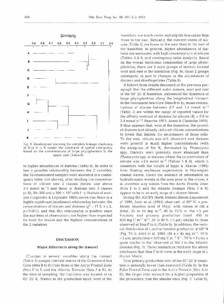
308 Mar. Ecol. Prog. Ser. 98: 297-313, 1993

Similarity

Fig. 9. Dendrogram showing the complete linkage clustering of Stns A to K (under the constraint of spatial contiguity), based on the concentrations of large phytoplankton in the

upper layer (Table 8)

to higher abundances of diatoms (Table 8). In order to test a possible relationship between the 2 variables, the 32 enumerated samples were allocated to a contingency table (not shown), after dividing the concentrations of sihcate into 2 classes (below and above 3.0 mm01 m-3) and those of diatoms into 3 classes (c 30, 30-300 and > 300 X 103 cells 1-l). Statistical analysis (Legendre & Legendre 1983) shows that there is a highly significant (nonlinear) relationship between the concentrations of silicate and diatoms ( x 2 = 17.5, v = 2, p <0.001), and that this relationship is positive since the numbers of observations are higher than expected for both the lowest and the highest concentrations of the 2 variables.

DISCUSSION

Major differences along the transect

Changes in several variables along the transect (Table 1) sharply contrast waters of the Greenland Sea Gyre (Stns B to E) from those of the Arctic Frontal Zone (Stns F to I) and the Atlantic Domain (Stns J & K). At the time of sampling, the transition was located at ca 05' 25' E. Waters m the production layer, west of the

transition, are much cooler and sllghtly less saline than those to the east. Similarly, the concentrations of silicate (Table 5) are lower to the west than to the east of the transition. In general, higher abundances of diatoms are associated with high concentrations of silicate (Tables 5 & 8, and contingency table analysis). Based on the overall taxonomic composition of large phytoplankton, there are 2 main groups of stations located west and east of the transition (Fig. 9); these 2 groups correspond in part to changes in the abundances of diatoms and dinoflagellates (Table 8).

It follows from results discussed in the previous paragraph that the different water masses, west and east of the 05' 25' E transition, influenced the dynamics of large phytoplankton along the longitudinal transect. In the Greenland Sea Gyre (Stns B to E), mean concentrations of silicate between 0.7 and 1.4 mm01 m-3 (Table 5) are within the range of reported values for the affinity constant of diatoms for silicate (K, = 0.8 to 3.4 mm01 m-3; Paasche 1973, Azam & Chisholm 1976). It thus appears that, west of the transition, the growth of diatoms had already reduced silicate concentrations to levels that limited the abundances of these cells. To the east, silicate was still abundant and diatoms were present in much higher concentrations (with the exception of Stn K, dominated by Phaeocystis spp). Diatoms were generally more abundant than Phaeocystis spp. at stations where the concentration of shcate was >2.6 mm01 m-3 (Tables 5 & 8), which is consistent with the results of Egge & Aksnes (1992) from floating enclosure experiments in Norwegian coastal waters. Given the absence of information on hydrodynamic events in the area prior to the cruise, it is uncertain why waters from the Arctic Frontal Zone (Stns F to I) and the Atlantic Domain (Stns J & K) appear to be in an early stage of a diatom bloom.

During the JGOFS North Atlantic Bloom Experiment of 1989, Joint et al. (1993) observed, at 60' N, a pre- bloom situation (end of May), with values of chl a (total: 35 to 50 mg m-*, 40 to 75% in the < 5 Fm fraction) and primary production (total. 450 to 830 mg C m-' d- l , 35 to 80 % i 5 pm) similar to those observed at Stns F to K (Table 6). In addition, the vertical distribution of size-fractionated production at 60" N (Fig. 7b in Joint et al. 1993; chl a = 45 mg m-', 70 %

c 5 pm; production = 520 mg C m-2 d-l , 70 % 1 5 pm) is quite similar to that observed at Stn J in the Atlantic Domain (Fig. 3). These similarities reinforce the above conclusion that Stns F to K were in the early stage of a diatom bloom.

Total primary production west of the 05' 25' E transition is generally lower than eastward (Table 6). In the Polar Frontal Zone and in the Arctic Domain (Stns A to D), the larger cells account for a higher proportion of the production than the smaller ones (Fig. 3, Table 6),

Legendre et al.: Environmental control of phytoplankton production in the Greenland Sea 309

while the situation is reversed in the Atlantic Domain (Stns J & K); between these 2 water bodies, in the Arctic Frontal Zone (Stns E & F), production profiles of the 2 size fractions are very similar. The magnitude of the subsurface production maxima (P,,,; Table 3) varies according to the oceanographic domains. The > 5 pm cells generally exhibit more pronounced production maxima in the Polar Frontal Zone and in the Arctic Domain (Stns A to F) than at stations to the east. The < 5 pm cells generally show more pronounced production maxima (Stns F to K) and higher P i (Stns H to K; Table 4, where maximum photosynthesis is estimated from Eq. 12) in the Arctic Frontal Zone and in the Atlantic Domain than at stations to the west. The observed change in primary production along the transect, from dominance by the > 5 pm fraction in the Polar Frontal Zone and the Arctic Domain to strong dominance by the < 5 pm fraction in the Atlantic Domain, thus corresponds to changes in the photosynthetic characteristics of the cells.

Production layer

The depth of the production layer (Table 2) seems to be primarily controlled by the underwater irradiance, since zprod is inversely correlated with the coefficient of diffuse light attenuation. At some stations, zProd also corresponds to the depth of the surface mixed layer (Stns C, E & H) or of the nutricline (Stns C, D & K), sug- gesting possible additional control of phytoplankton production on the vertical through hydrodynamics.

In general, irradiance at the bottom of the production layer EI(zprod) is 1 5 pEin m-2 S- ' . Compensation irradiance~ for photosynthesis, measured in the laboratory for chl a-, c- and carotenoid-containing algae, range between 0.2 pEin m-2 S-' (Skeletonerna costa- turn; Falkowski & Owens 1980) and values that vary from 4 to 20 (Dunaliella tertiolecta; Falkowski & Owens 1980) or 5 to 20 (Arnphidiniurn carterae; Samuelsson &

Richardson 1982) depending upon the irradiance under which the algae were grown (Richardson et al. 1983). At most of the sampling stations, the bottom of the production layer therefore probably corresponds to the compensation depth for phytoplankton photosynthesis (i.e. the depth where phytoplankton production is balanced by respiration).

Environmental control of primary production

With the exception of Stns A & C, all the sampled stations experienced relatively similar daily average irradiance in the production layer (from 2.4 to 4.6 Ein m-' d-'; Table 2). The attenuation of light in the

water column at the sampled stations is largely determined by phytoplankton and phytodetritus, i.e. the mean concentration of pigments (chl a + Phaeo) in the production layer accounts for >65 "/o of the observed variation in the coefficient of diffuse light attenuation. In general, the vertical distribution of irradiance E(z) accounts for most of the variation in measured PB(z) within the production layer (Table 4). This is especially true for the > 5 pm fraction, where E(z) accounts for r2 = 60 to 97 % of the variance in PB(z) and where all the nonlinear correlations between the 2 variables are significantly different from zero. For the < 5 pm fraction, some of the stations (B, D, F & K) do not exhibit such a straightforward relationship between photosynthesis and irradiance, while the others have r2 as high as for the > 5 pm fraction. In addition, maximum photosynthetic activity in the water colunln (P;), for the > 5 pm fraction, is significantly correlated with E(z,) taking into consideration all the stations where the latter is defined. Also, activity of the photosynthetic biomass in the lower part of the production layer is generally reduced (Fig. 6). Finally, subsurface production maxima for the total samples and the 2 size fractions (Figs. 2 & 3) are always shallower than the maxima or sharp decreases in subsurface chlorophyll (when present; Figs. 4 & 5).

The characteristics of phytoplankton production summarized in the previous paragraph suggest that, in the lower part of the production layer, the photosynthetic biomass is limited by irradiance. This situation is similar to that reported by Herman & Platt (1986) for the Scotian Shelf (Eastern Canada), where subsurface production maxima often occurred within the upper chlorophyll gradient. They concluded that much of the subsurface chlorophyll was probably not photosynthetically active, due to limitation by irradiance. Size- fractionated samples (Table 4) show that P: of cells > 5 pm are systematically higher than those of cells < 5 pm, and that maximum photosynthetic activity for cells < 5 pm always occurs at a lower irradiance (i.e. deeper) than for either the > 5 pm cells or the total samples. This may be explained by higher photosynthetic efficiency, at low irradiance, for picoplankton than for the larger cells (e.g. Glover & Morris 1981, Platt et al. 1983, Glover et al. 1985).

Primary production, standing stock and ecosystem

types

Values of area1 total primary production in Table 6 (350 to 960 mg C n r 2 d - ' ) are consistent with estimates ("N uptake) at the end of May, published by Keene et al. (1991) for the East Greenland Polar Frontal Zone (76 to 78' N, 6' W to 4' E; 776 mg C m-2 d-l) and the

310 Mar. Ecol. Prog. Ser. 98: 297-313, 1993

Arctic Frontal Zone (74 to 75" N, 4 to 8' E; 215 mg C m-2 d-l). They are also consistent with I4C uptake measurements, reported in Hirche (1988) for the area corresponding to Stns E to I (74 to 75" N, 4 to 9" E; their Stns 72 to 94; 330 to 635 mg C m-' d-l). At these stations, the fraction c 2 0 Frn accounts for 25 to 47 % of the total production, which is similar to the contribution of the < 5 pm fraction at Stns E to 1 (50 to 55 %; Table 7). As observed by Smith et al. (1991) at 78" 30' N in April and May, the high rates of primary production are not limited to areas close to the ice edge, but occur at most stations (especially in the Arctic Frontal Zone; Stns F to I, Table 6). However, high production is not always associated with high concentrations of Phaeocystis spp. (Tables 6 & 8), contrary to the situation reported by Smith et al. (1991) earlier in the season (April-May).

Maximum concentrations of phycoerythrin-containing cyanobacteria in the vertical profiles (Fig. 8) are 3.7 to 14.6 X 105 cells 1-' at Stns A to E (-0.8 to 0.6'C), and 2.9 to 17.8 X 105 cells 1-' at Stns F to K (3.0 to 6.5"C). These values are intermediate between maximum concentrations from vertical profiles observed near Iceland (61 to 63' N; 2 to 16 X 106 cells 1- l ) by Murphy & Haugen (1985), and abundances < 23 X 103 cells 1-' reported in the ice-covered East Greenland Current (Fram Strait; 80 to 81' N) by Gradinger & Lenz (1989). Present results thus confirm the general trend from these previous studies of a progressive decrease of phycoerythrin-containing cyanobacteria with increasing latitude, in the North Atlantic. The dfference in concentrations between stations west and east of the 05' 25' E transition would support the conclusion of the above cited authors that water temperature may play a role in controlling the abundance of cyanobacteria. Maximum concentrations of small chlorophyll-containing eukaryotes in the vertical profiles range between 1.2 X 106 (Stn G) and 11.3 X 106 (Stn E) cells 1-l. These are similar to maximum concentrations from vertical profiles near Iceland (6 to 16 X 106 cells 1 - l ) , which is consistent with the observation of Murphy & Haugen (1985) that small eukaryotes dominate the ultraphytoplankton in the ocean at high latitude. For comparison, in the isothermal layer (> 12 "C) of vertically stable waters <50° N, these authors report that cyanobacteria were ca 1 order of magnitude more abundant than the small eukaryotes.

Estimates of potential sedimentation (S) and grazing (g) rates in Table 7 are derived from a simple model (see the 'Materials and methods'), in which all the primary production is exported out of the production layer, in the form of intact cells (chl) and faecal pellets (Phaeo). In the same region (74 to 75' N, 4 to 8' E) at the end of May, Keene et al. (1991) estimated the I-ratio (ratio of new to total primary production) to

be 0.69. Within the context of the steady-state stoichio- metric model of Eppley & Peterson (1979), this would indicate that ca 70% of the primary production was available for export from the euphotic zone. Given this high export potential in the sampled area, the present model, which assumes 100 % export, may thus provide useful indications concerning potential export pro- cesses.

One of the simplifying assumptions of the model is that all grazed chl a is transformed into Phaeo. This assumption has been criticized in the Literature (e.g. Conover et al. 1986, Lopez et al. 1988, Pasternak & Drits 1988). Combining Eq. (16) with Eqs. (17 to 19) gives:

g c h l - S Phaeo = 0

If only part of the grazed chl a had in fact been con- verted into Phaeo, [g chl] would overestimate the actual production of Phaeo (pPhaeo Phaeo = g chl; Eq. 18), so that true S should be smaller than calculated. In such a case, true g would be larger than calculated, in order to satisfy Eq. (15) (combined with Eqs. 17 & 19):

It follows that potential grazing rates calculated with Eq. (21) might underestimate actual grazing, and that potential sedimentation rates calculated using Eq. (20) might overestimate actual sedunentation. The real differences between sedimentation and grazing rates may therefore be smaller than those shown in Table 7.

In addition, it could be argued that larger calculated sedimentation and grazing rates for the > 5 l m fraction, in cases where this fraction accounts for a large part of the production, may simply reflect the fact that the 2 rates are linked to primary production through the following relation:

which is another formulation of the steady state assumption, i.e. export = production. However, the parti- tioning of production between potential sedimentation and grazing in Eqs. (20 & 21) depends on the relative abundances of chl a and Phaeo, so that there is no significant relationship between percent production by the > 5 pm cells (Table 6) and either sedimentation or grazing rates (Table 7) (r = 0.41 and 0.57, respectively, p > 0.05). The much higher potential grazing rates at Stns A, C and D therefore probably reflect a real difference in grazing for these stations, within the context of the simplifying assumptions stated in the 'Materials and methods' (Eqs. 17 to 19).

Legendre et al.: Environmental control of ph ~ytoplankton production in the Greenland Sea 311

Legendre & Le Fevre (1991) proposed a typology of pelagic marine ecosystems, based on 5 combinations linking the size distribution of phytoplankton production to that of the standing stock. Stations sampled during the present study correspond to 2 of these types: i.e. ( l ) production as well as standing stock dominated by small cells (Stns J & K ) ; and (2) production by large and small cells but standing stock dominated by small cells (Stns A to 1). Other possible types (not encountered in the present study) are: production by large and small cells and standing stocks dominated by either (3) large and small cells or (4) large cells, and (5) production as well as standing stocks dominated by large cells.

According to Legendre & Le Fevre (1991), the various types of ecosystems correspond to different modes of phytoplankton production (determining the size distribution of production) and different trophic structures (as reflected in the size distribution of the standing stock). They explain that efficient export of large cells, through grazing and sedimentation, is responsible for the dominance of the standing stock by small phytoplankton in cases where production is affected by both large and small cells. It is thus expected that grazing on the large cells should be strong when there is a large difference between the proportions of the production and of the biomass accounted for by the large cells. This is what occurs at Stns A, C & D , where there are large positive differences (17 to 29 %) between the proportions of production and chl a biomass accounted for by cells > 5 pm (Table 6) and where, in agreement with Legendre & Le Fevre (1991), potential grazing on cells > 5 pm is more than 2.5 times that on cells < 5 pm (Table 7).

Two stations exhibit a negative difference between the proportions of production and biomass accounted for by cells > 5 pm (Stns B & K; Table 6, Fig. 7). This may be interpreted as reflecting accumulation of the large phytoplankton in the production layer. Interestingly, these 2 stations are also those with the largest proportions of Phaeocystis spp. (Table 8). Concentrations of Phaeocystis spp. at the sampling stations are within the range of values reported by Smith et al. (1987) for the marginal ice zone of the Fram Strait ( 2 to 8125 X 103 cells I- '). There are reports of large blooms of Phaeocystis spp. in the marginal ice zone (e.g. Smith et al. 1987 and references therein, Gradinger & Baumann 1991, Hirche et al. 1991) and also in waters remote from the ice edge (Smith et al. 1991). High concentrations observed at Stn B may correspond to the former, while those at Stn K may pertain to the latter. Such blooms may be subjected to active grazing by micro-, meso- and possibly macrozooplank- ton (references in Sournia 1991). At Stn B (Table 7), the potential grazing rate on phytoplankton > 5 pm (prob-

ably largely Phaeocystis spp.) is not the lowest observed and, at Stn K , it is the highest of all the stations. This is consistent with grazing on Phaeocystis spp. In contrast, potential sedimentation rates of cells > 5 pm are especially low at Stns B & K, which suggests that the accumulation of large phytoplankton there may reflect low sedimentation of Phaeocystls spp. However, according to conditions, Phaeocystis spp. aggregates may sometimes rapidly sink out of the euphotic zone (e.g. for Arctic waters, see Wassmann et al. 1990).

Given the above discussion, water bodies sampled during the cruise could be ecologically characterized as follows (Tables 7 & 8, Fig. 7). In the Polar Frontal Zone and the Arctic Domain (Stns A to D), primary production is generally dominated by cells > 5 pm (up to 66 %), but this is not proportionally reflected in the standing stock (Stns A, C & D are located far from the diagonal in Fig. 7), potentially due to strong grazing on the large cells; sedimentation of cells > 5 pm may also be high relative to cells <5 pm. In the Arctic Frontal Zone (Stns E to I) , production is equally shared by the large and small size fractions, but the standing stock is still dominated by cells 5 pm; potential rates of grazing and sedimentation of large versus small cells are generally lower than in the Arctic Domain. In the Atlantic Domain (Stns J & K), both primary production and standing stock are largely dominated by cells < 5 pm. The 2 stations where the biomass of large cells is dominated by Phaeocystis spp. (Stns B & K) may be characterized by low sedimentation of large cells relative to that of small ones.

Acknowledgements. This research was funded by grants to L.L. from the Natural Sciences and Engineering Research Council of Canada, and to GIROQ (Groupe interuniversitaire de recherches oceanographiques du Quebec) from NSERC and the Fonds FCAR of Quebec. We thank U. Babst, H. Becker, G. Bergeron, M.-J Mai-tineau, U. Meyer, M. Stiircken and K. Pfeifer for assistance in the field, E. M. Haugen for help with epifluorescence microscopy, S. Gugg and S. Higgins for ultraphytoplankton enumeration, L. Berard-Therriault for Utermohl phytoplankton enumeration, H. Becker, S. Gosselin, D LeBlanc and M. Parrot for data analyses, and anonymous reviewers for useful suggestions. Contribution to the programme of GIROQ, and contribution no. 591 of the Alfred-Wegener-Institut fiir Polar- und Meeresforschung.

LITERATURE CITED

Anonymous (1989). Sun. In: The astronomical almanac 1989. U.S. Government Printing Office. Washington, DC, Cl-C24

Azam, F., Chisholm, S. W. (1976). Silic~c acid uptake and in- corporation by natural manne phytoplankton populations. Limnol. Oceanogr 21: 427-435

312 Mar. Ecol. Prog. 6

Baumann. M. (1990). Untersuchung zur Primarproduktion und Verteilung des Phytoplanktons der Gronlandsee mit Kulturexperi.menten zum EinfluB des Lichtes und der Temperatur auf Wachstum und Photosyntheseleistung arktischer Diatomeen. Ph.D. thes~s, RWTH Aachen

Chu, P. C., Gascard. J. C. (eds.) (1991). Deep convection and deep water formation in the oceans Elsevier, Amsterdam

Coachman, L. K., Aagaard, K. (1974). Physical oceanography of Arctic and subarctic seas. In: Herman, Y (ed.) Marine geology and oceanography of the Arctic seas. Springer- Verlag, New York, p. 1-72

Conover, R. J., Durvasula, R., Roy, S., Wang, R. (1986). Probable loss of chlorophyll-derived pigments during passage through the gut of zooplankton, and some of the consequences. Limnol. Oceanogr. 31: 878-887

Cooper, P. I. (1969). The absorption of solar radiation in solar stills. Sol. Energy 12: 333-346

Egge, J . K. , Aksnes, D. L. (1992). Silicate as regulating nutrient in phytoplankton competition. Mar. Ecol. Prog. Ser. 83: 281-289

Eppley, R. W., Peterson, B. J . (1979). Particulate organic mat- ter flux and planktonic new production in the deep ocean. Nature 282: 677-680

Falkowski, P. G., Owens, T. G. (1980). Light-shade adaptation. Two strategies In marine phytoplankters. Plant Physiol. (Bethesda) 66: 592-595

Glover, H. E., Morris, 1. (1981). Photosynthetic characteristics of coccoid marine cyanobacteria. Arch. Mikrobiol. 129: 42-46

Glover, H. E., Phinney, D. A., Yentsch, C. S. (1985). Photosynthetic characteristics of picoplankton compared with those of larger phytoplankton populations, in various water masses in the Gulf of Maine. Biol. Oceanogr. 3: 223-248

Gradinger, R . , Lenz, J. (1989). Picocyanobacteria in the high Arctic. Mar. Ecol. Prog. Ser. 52: 99-101

Gradinger. R. R.. Baumann. M. E. M. (1991). Distribution of phytoplankton communities in relation to the large-scale hydrographical regime in the Fram Strait. Mar. Biol. 111: 311-321

Hall, J . A.. Vincent. W. F. (1990). Vertical and horizontal structure in the picoplankton communities of a coastal upwell- ing system. Mar. Biol. 106: 465-471

Hebbeln, D., Wefer, G. (1991). Effects of ice coverage and ice- rafted material on sedimentation in the Fram Strait. Nature 350: 409-41 1

Herman, A. W., Platt, T. (1986). Pnmary production profiles in the ocean: estimation from a chlorophyll/light model. Oceanol. Acta 9: 31-40

Hirche, H. J . (ed.) (1988). Data report of RV 'Polarstern' cruise ARK IV/1, 1987, to the Arctic and Polar Fronts. Ber. Polarforsch. 44: 1-228

Hirche. H. J . , Baumann. M. E. M., Kattner, G , Gradinger, R. (1991). Pl.ankton d.istnbution and the impact of copepod grazing on primary production in Fram Strait, Greenland Sea. J. mar. Syst. 2: 477-494

Joint, I . , Pomroy, A., Savidge, G., Boyd, P. (1993). Size-fractionated pnmary productivity in the northeast Atlantic in May-July 1989. Deep Sea Res. 40: 423-440

Kattner, G., Becker, H. (1991). Nutrients and organic nitro- genous compounds In the marginal ice zone of the Fram Stra~t . J . mar. Syst. 2. 385-394

Keene, N. K., Smith, W. 0. Jr, Kattner, G. (1991). Nitrogen uptake in two frontal areas in the Greenland Sea. Polar Biol. 11. 219-225

Kirk. J. T 0 . (1983). Light and photosynthesis in aquatic ecosystems. Cambridge Univ. Press. Cambridge

Legendre, L., Demers, S., Yentsch. C. Wl., Yentsch, C. S. (1983). The "C method: patterns of dark CO2 fixation and DCMU correction to replace the dark bottle. Limnol. Oceanogr. 28: 996-1003

Legendre. L., Le Fevre, J. (1989). Hydrodynamic singularities as controls of recycled versus export production in oceans. In: Berger, W. H., Smetacek, V. S., Wefer, G. (eds.) Productivity of the ocean: present and past. Wiley, Chichester, p. 49-63

Legendre, L., Le Fevre, J. (1991). From individual plankton cells to pelagic marine ecosystems and to global biogeochemical cycles. In: Demers, S. (ed.) Particle analysis in oceanography. Springer-Verlag. Berlin, p. 260-299

Legendre, L., Legendre, P. (1983). Numerical ecology. Elsevier, Amsterdam

Lopez, M. D. G., Huntley, M. E., Sykes, P. F. (1988). Pigment destruction by Calanus pacificus: impact on the estimation of water column fluxes. J. Plankton Res. 104: 715-734

Lund, J. W. G., Kipling, C., Le Cren, E. D. (1958). The inverted microscope method of estimating algal numbers and the statistical basis of estimations by counhng. Hydrobiologia 11: 143-170

Murphy. L. S., Haugen. E. M. (1985). The distribution and abundance of phototrophic ultraplankton in the North Atlantic. Limnol. Oceanogr. 30: 47-58

Paasche, E. (1973). Silicon and the ecology of marine diatoms. 11. Silicate-uptake kinetics in five diatom species. Mar. Biol 19: 262-269

Paquette, R. G., Bourke, R. H., Perdue, W. F. (1985). The East Greenland Polar Front in autumn. J . geophys. Res. 90: 4866-4882

Parsons, T R. , Maita, Y., Lalli, C. M. (1984). A manual of chemical and biological methods for seawater analysis. Pergamon Press, Toronto

Pasternak, A. F., Drits, A. V. (1988). Possible degradation of chlorophyll-derived pigments during gut passage of herbivorous copepods. Mar. Ecol. Prog. Ser. 49: 187-190

Platt, T., Gallegos, C. L . , Harrison, W. G. (1980). Photo- inhibition of photosynthesis in natural assemblages of marine phytoplankton. J. mar. Res. 38: 687-701

Platt, T., Subba Rao, D. V., Irwin, B. (1983). Photosynthesis of picoplankton in the oligotrophic ocean. Nature 301: 702-704

Price, N. M., Harrison, P. J. (1987). Comparison of methods for the analysis of dissolved urea in seawater. Mar. Biol. 94: 307-313

Richardson, K., Beardall, J., Raven, J. A. (1983). Adaptation of unicellular algae to irradiance: an analysis of strategies. New Phytol. 93: 157-191

Sakshaug, E , Slagstad, D. (1991) Light and productivity of phytoplankton in polar marine ecosystems: a physiological view. Polar Res. 10: 69-85

Samuelsson, G., Richardson, K. (1982). Photoinhibition at low quantum flux densities in a marine dinoflagellate. Mar. Biol. 70: 21-26

SAS (1982). SAS user's guide. statistics, 1982 edn. SAS Institute, Inc., Cary, NC

Smith, S. L.. Smith, W. 0. Jr, Codispoti, L. A., Wilson, D. L. (1985). Biological observations in the marginal ice zone of the East Greenland Sea. J . mar. Res. 43: 693-717

Smith, W. 0. Jr, Baumann, M. E. M, , Wilson, D. L., Aletsee, L. (1987). Phytoplankton biomass and productivity in the marginal ice zone of the Frarn Strait during summer, 1984. J . geophys Res. 92: 6777-6786

Smith. W. 0. Jr, Codispoti, L. A., Nelson, D. M,. ~Manley, T., Buskey, E. J., Niebauer, H. J. , Cota, G. F. (1991).

Legendre et a1 . Environmental control of phytoplankton production in the Greenland Sea 313

Importance of Phaeocystis blooms in the high-latitude ocean carbon cycle. Nature 352: 514-516

Smith. W. 0. Jr. Kattner, G. (1989). Inorganic nitrogen uptake by phytoplankton in the marginal ice zone of the Fram Strait Rapp. P.-v. Reun. Cons. int. Explor Mer 188: 90-97

Sournla, A (1991). Le genre Phaeocystis (Prymnesiophycees). In: Sourn~a , A . et al. (eds.) Le phytoplankton nuisible des cBtes de France: de la biologie a la prevention. IFREMER, Brest, p. 91-100

Sples, A (1987). Phytoplankton in the marginal ice zone of the Greenland Sea during summer, 1984. Polar Biol. 7: 195-205

This article was submitted to the editor

Swift, J. H. (1986). The Arctic waters. In: Hurdle, B. G. (ed.) The Nordic seas. Springer-Verlag, New York, p. 129-153

Swift. J. H., Aagaard, K. (1981). Seasonal trans'itions and water formation in the Iceland and Greenland Seas. Deep Sea Res 28: 1107-1129

Miassmann, P , Peinert, R., Smetacek, V (1991). Patterns of production and sedimentation in the boreal and polar Northeast Atlantic. Polar Res. 10 209-228

Wassmann, P., Vernet, M, , Mitchell, G , Rey, F (1990). Mass sedimentation of Phaeocystispoucheti~ In the Barents Sea. Mar. Ecol. Prog. Ser. 66: 183-195

Manuscript first received: February 5,1993 Revised version accepted: April 5,1993

environmental control and potential fate of size

Documents