Charles University in Prague, Faculty of Science, Institute for Environmental Studies

SPATIAL ANALYSIS FOR ENVIRONMENTAL MAPPING

OF ŠUMAVA NATIONAL PARK

Lemenkova Polina

2

• Planned PhD work: Assessment of natural and human-induced changes in the vegetation of important floristic locations in South-West Bohemia: a GIS analysis

• Results of the 1st year include: 1. Literature review of the research area (geography,ecological settings,

botanical characteristics, environmental problems etc) 2. Data capture from various sources 3. Technical organizing of GIS project, compatibility of data. 4. Remote sensing data processing and spatial analysis

!• Current presentation shows these results (1st part of the PhD work, year

1): “Remote sensing data analysis for pattern recognition of the land cover types in Šumava National Park (time span 1991-2009)”.

Content of Presentation

3

Structure of PresentationCurrent presentation consists of 2 parts: !1) Overview of the environmental research problem and biogeographical characteristics of Šumava National Park. Consequences of anthropogenic and climatic impacts on land cover patterns !2) Detailed technical description of the workflow (GIS part): remote sensing data capture, pre-processing, algorithm processing, image classification and spatial analysis. !The presentation is formed by 46 slides, two logical parts. • Part 1 (ecological overview of study area): 12 slides, • Part 2 (GIS spatial analysis workflow): 34 slides. !Proposed time: 15 min (~3 slides / min)

Summary

Research area: Šumava National Park, Czech Republic, spatial segment of 48°-49° N, 12°-13° E !Research aim: spatio-temporal analysis of land cover changes in study area during 18 years (1991-2009) !Research objective: application of geoinformatic tools of QGIS, remote sensing data (satelite images Landsat TM) and spatial analysis methodology for ecological study

Part I

Part I: Environment and Geography of the Study Area

Study Area: Overview

Significance: Since 1990 the Šumava National Park (further ŠNP) has been the protected Biospherical Reserve of UNESCO and Natura 2000 protected area: the Bird EU Directive and Habitat EU Directive

Characteristics: the fundamental features of ŠNP include its topographic location in 3 boarding countries (Czech Republic, Germany and Austria) and climatic-geographic settings. The study area is the largest of the four national parks (68,064 hectares) located in the south-west of Czech Republic, on the border with Germany.

Fig.1.

7

Geographic LocationTopographically, the ŠNP spreads from the northeast to the southeast. It is

located at the heights between 600 m (Otava River valley at Rejštejn) and

1378 m (top Plechý, the highest mountain of the Czech Bohemian Forest). The highest peak on the Czech

side is mountain (1456 m).

Geomorphologically, the study

area covers Šumava plains,

u p l a n d s Ž e l e z n o r u d s k o ,

Boubínská , Želnavskou , the

Šumava mountains and Vltava

furrow (Barešová & Hanusová,

2010).

Fig.2.

8

Hydrological SettingsThe ŠNP is the principal European division between the North and the Black

Sea. Hydrologically, it includes most of the drainage area (springs and bogs,

rivers, glacial lakes and artificial waters) to the North Sea, the Elbe River

Basin with major rivers Vltava and Otava.

The ŠNP is included in the protected areas of natural water accumulation (CHOPAV), designed to prevent the reduction of the water potential, and negative changes in water quality and conditions. Climatic settings, wetlands, peatlands and forests affect positively the accumulation of water in the area and their control runoff.

Hydrological network visualization

Fig.3.

9

Geobotanical Settings

Geobotanically, the ŠNP belongs to the Bohemian Forest, which is split into

two national parks (Czech Republic and Germany). It forms a unique

protected forested area in Central Europe and one of the largest forested areas

between the Atlantic Ocean and Ural (Krenova and Hruska, 2012). The habitats of the

ŠNP are represented

by diverse biotops and

host numerous rare

and protected flora

and fauna species.

Natura-2000 zonation

Geobotanical zonation

Fig.4. Fig.5.

10

Vegetation Zones

• vast wooded areas, • mountain spruce forests • fir-beech and spruce fir-beech • mixed forests of various ages, • peat bogs, grasslands, heaths, debris, • meadows biotops, secondary shrubs • moors, lakes, streams, springs, wetlands • habitats modified or affected by humans

The area is represented by following main vegetation types:

Altogether, they create a unique mosaic of biotopes, which is a

habitat for a variety of rare, endemic and endangered species,

e.g. lynx, pearl mussel, owls, diverse songbirds, etc.

11

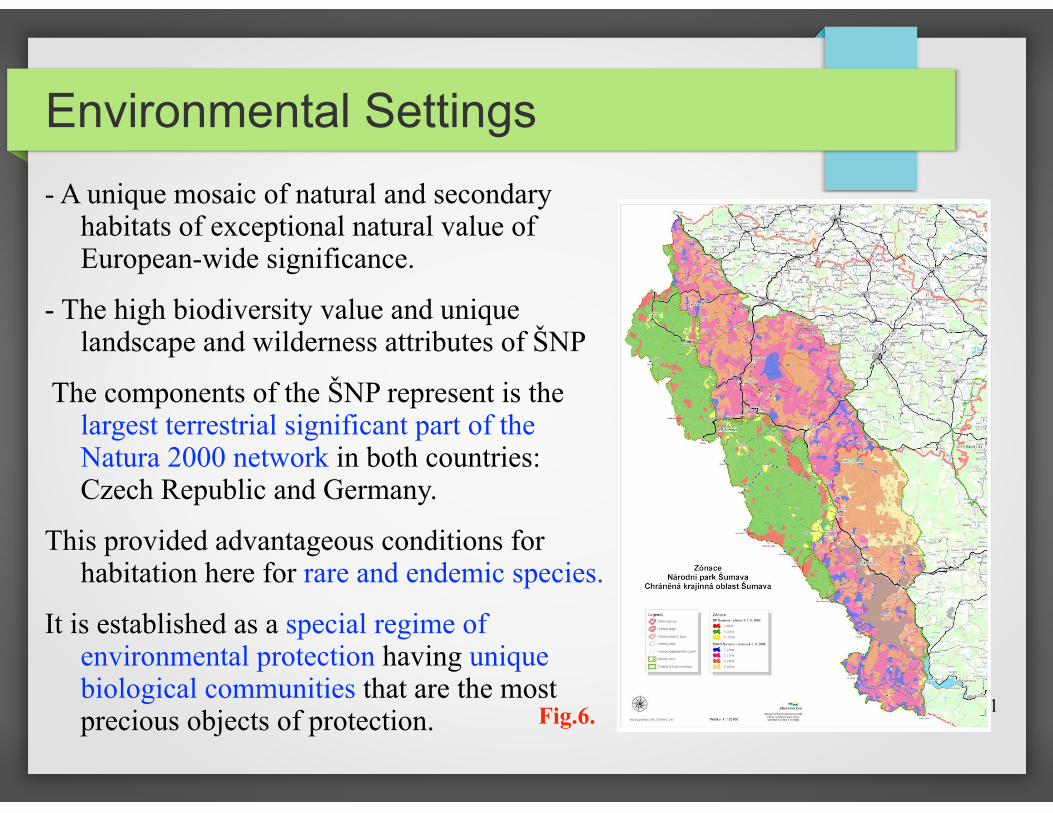
Environmental Settings- A unique mosaic of natural and secondary

habitats of exceptional natural value of European-wide significance.

- The high biodiversity value and unique landscape and wilderness attributes of ŠNP

The components of the ŠNP represent is the largest terrestrial significant part of the Natura 2000 network in both countries: Czech Republic and Germany.

This provided advantageous conditions for habitation here for rare and endemic species.

It is established as a special regime of environmental protection having unique biological communities that are the most precious objects of protection. Fig.6.

Examples of Environmental Problems

• Human activity reached its peak at the end of the 19th and beginning of the 20th century. During that period, the original floodplain forests were fragmented and deforested land was managed mostly as regularly-cut meadows (Schreiber 1924, Holubicková 1960).

• During last decades some ecosystems components are being gradually, changed, or degrading, or under extinction. For example, the number of populations of rare plant species Gentianella praecox subsp. bohemica. (endemic to semi-natural grasslands in central Europe) declined rapidly in the last 60 years (Bucharová et al. 2012).)

• The extinction of some endangered, rare, unique and important species can be inevitable within several decades without management: even very large populations (1000 flowering individuals) can disappear before 2060

• The future of nature conservation in the ŠNP caused discussions about zoning of the Park, which has undergone significant changes since establishment (Křenová and Hruška 2012).

Part II

Part II: Remote Sensing Data

using Quantum GIS

Methods

1)Data capture, unpacking and storage. 2)Organizing GIS project. 3)Geo-referencing and re-projection. 4)Activating GDAL and GRASS remote sensing plugins. 5)Preliminary data processing. 6)Generating contour layers from DEM 7)Color composition from 3 Landsat TM bands 8)Defining Region of Interest: raster mosaicing and clipping 9)False color composites (bands 4-3-2) 10)Setting up parameters for classification 11)Image classification using K-Means algorithm 12)Pattern recognition 13)Spatial analysis

Methods used in the current work include following steps:

Techniques

● The research was performed using Quantum GIS (QGIS) software using Landsat TM images for 1991 and 2009 (18-year time span).

● The landscapes in study area at both Landsat TM images were classified into different land cover types

● The area covered by each land cover class is compared and dynamics is analyzed for respecting years.

● The changes in the selected land cover types were analyzed and the environmental modifications within landscapes detected.

● Finally, classified land cover types across study area were compared at both maps of land cover types for the years 1991 and 2009, respectively.

16

Data Content. Vector Layers.The data used in the current work consist of 2 parts: vector and raster layers. !

Geodetic background of vector layers: the data were stored in a GIS Project with the following coordinate system and mathematic projection: World Geodetic System WGS 84, ellipsoid Bessels, Křovák's Projection with 2 pseudo-standard parallels (oblique case of Lambert conformal conic projection made in 1922 for Czech Republic)

Content: basic and geographic

info: hydrological network,

municipalities and cities, roads,

borders, relief, geomorphic

contours, zone boundaries,

NATURA 2000, etc.

Vector layers: GIS layers used for the spatial

analysis include various vector layers in ArcGIS

shape-file (.shp) format. Fig.7.

17

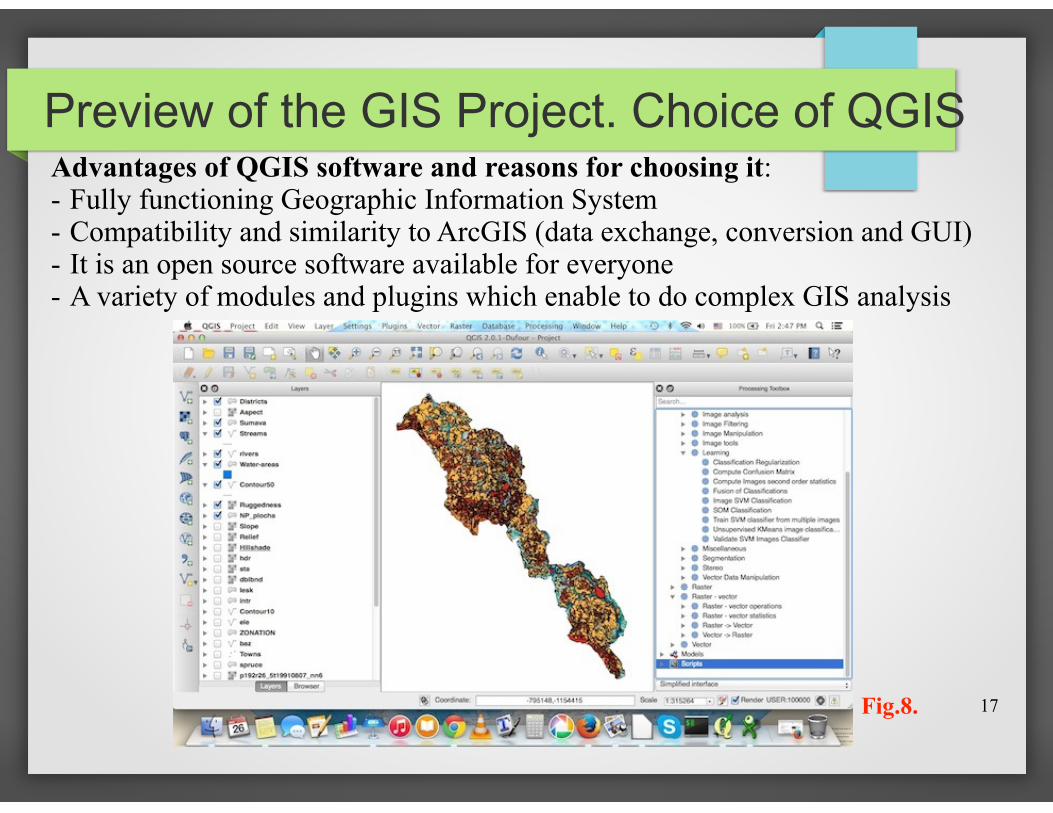
Preview of the GIS Project. Choice of QGISAdvantages of QGIS software and reasons for choosing it: - Fully functioning Geographic Information System - Compatibility and similarity to ArcGIS (data exchange, conversion and GUI) - It is an open source software available for everyone - A variety of modules and plugins which enable to do complex GIS analysis

Fig.8.

Data Capture. Raster Layers.Two Landsat Thematic Mapper (TM) images were downloaded from the Global Land

Cover Facility Earth Science Data Interface website (http://glcfapp.glcf.umd.edu ).

To select target area, a spatial mask of coordinates ranging from 48°00’-49°00’N, 12°00’-13°00’E.

The target images were chosen on 1991 and 2009 years due to 3 reasons (reasonable time span of 18 years, summer period, technical availability of cloudless images).

Capture of Landsat TM, 2009Capture of Landsat TM, 1991

Fig.9. Fig.10.

19

Cloud CoverageThe main important issue for remote sensing (RS) data:

“the less clouds the better”.

Other point for vegetation classification is “clouds nature and their location”: images with clouds above non-forest (urban) area is Ok, but clouds above forest area make otherwise good image useless.

Landsat TM, 1991-08-07 Landsat TM, 2001-08-26 Landsat TM, 2009-08-24

Fig.12.Fig.11. Fig.13.

Data Unpacking and StorageThe Landsat search parameters were tailored using GLCF website: • selecting a region on a map, • entering coordinates, and • entering a place name (Šumava National Park) Additionally, the option to choose data set was used (“Landsat 4-5 TM”, “Landsat Orthorectified ETM+”) and then parameters of acceptable cloud-cover % and the range of desired acquisition dates were selected. After that using the provided path (Fig. left) the data were downloaded. Final step includes data unpackage and storage (two bottom figures).

Fig.14.

Fig.15. Fig.16.

21

Data Preview

Landsat TM, 1991-08-07 Landsat TM, 2009-08-24

Fig.17 Fig.18

22

Changing Geographic Coordinate System

+proj=krovak +lat_0=49.5 +lon_0=24.83333333333333 +alpha=0 +k=0.9999 +x_0=0 +y_0=0 +ellps=bessel +towgs84=589,76,480,0,0,0,0 +units=m +no_defs

To change projection of Landsat TM sciences I enabled “on the fly” projection by clicking on the CRS Status button in the Status Bar and chose Enable ‘on the fly’ CRS transformation

Fig.19.

Fig.20.

RS Data Read Into ProjectFig.21

24

Landsat TM Satellite ImagesThe dataset includes the metadata file and the following Landsat TM

spectral bands (16 bit raster) with a spatial resolution of 30 meters:

Band 1 = Blue; Band 2 = Green; Band 3 = Red; Band 4 = Near-Infrared; Band 5= SWIR (Short Wavelength Infrared 1); Band 6 = Thermal Band 7 = SWIR (Short Wavelength Infrared 2).

Table Source: http://landsat.usgs.gov/

25

Activating RS Tools in QGIS

To activated remote sensing (RS) functioning, I activated and updated the GDAL and GRASS plugins (figure below) using the “Manage Plugins” (Plugins menu) and selected all useful ones.

After that the GUI changed to active image processing menu (next step)

New activated functions of remote sensingActivation of plugins

26

The GeoTiffs of all Landsat layers were loaded into project one by one as separate raster layers.

To apply contrast enhancements, the minimum and maximum display values were set in properties by double clicking the layer name.

Preliminary Data Processing

These settings were used from the Symbology menu in the Layer Properties window that appears.

Transparency, raster histogram, zoom pyramids, metadata and other information and settings were adjusted from the Layer Properties window (Fig. right).

27

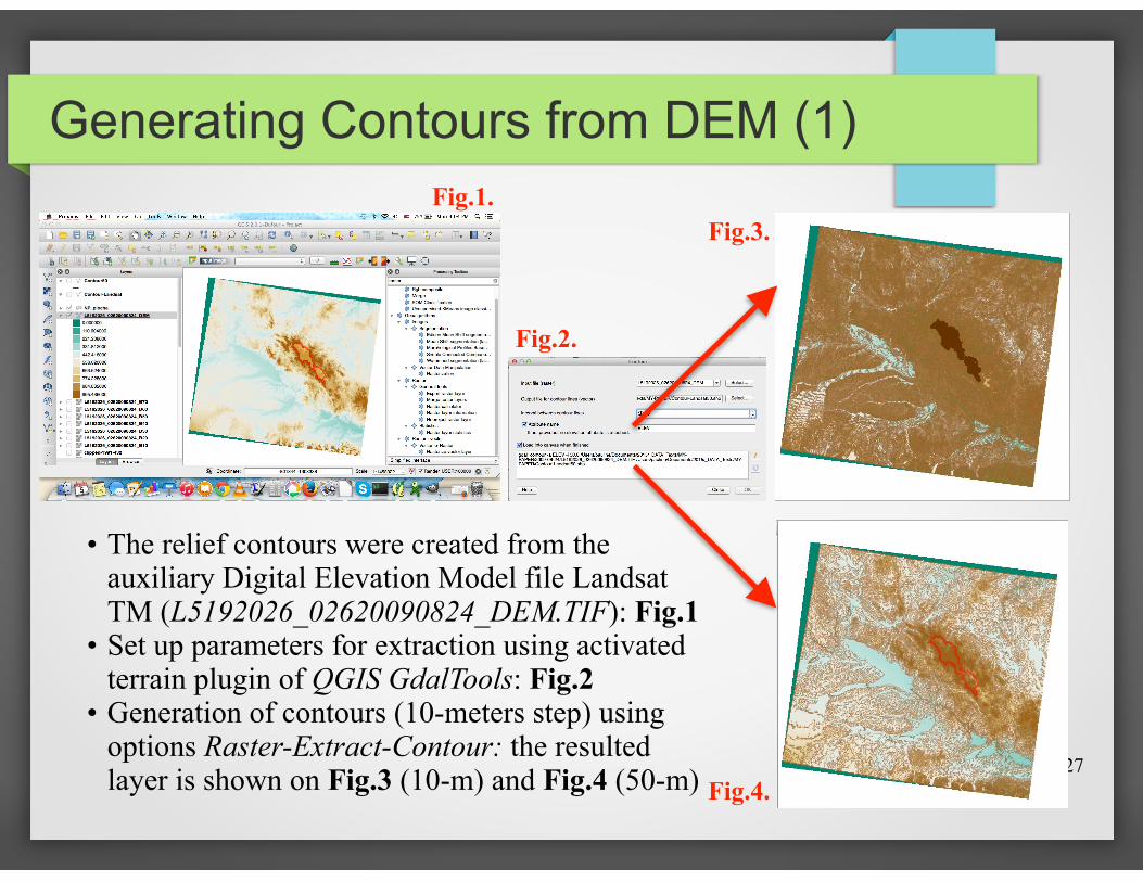
• The relief contours were created from the auxiliary Digital Elevation Model file Landsat TM (L5192026_02620090824_DEM.TIF): Fig.1

• Set up parameters for extraction using activated terrain plugin of QGIS GdalTools: Fig.2

• Generation of contours (10-meters step) using options Raster-Extract-Contour: the resulted layer is shown on Fig.3 (10-m) and Fig.4 (50-m)

Fig.1.

Fig.2.

Fig.3.

Fig.4.

Generating Contours from DEM (1)

28

• Next step was clipping the contours using mask of study area and repeating the same procedure for contours with 50 meters step: Fig.1 and Fig.2

• The generated relief is shown on Fig.3. and Fig.4 of current slide

Generating Contours from DEM (2)

Relief of study area

Generated geomorphological contours (50 m)

Fig.2.

Fig.1.

Fig.3.Fig.4.

29

Creating False Color CompositeTo create false color composites from two images I used combination of

bands 4-3-2, i.e. combination of: • band 4 VNIR (Visible Near Infra Red)- 0.76 - 0.90 µm • band 3 red - 0.61 - 0.69 µm • band 2 green - 0.51 - 0.60 µm These three bands are usually being merged for 'traditional' false color

composite. This false color combination (4-3-2) makes vegetation appear as reddish colors.

A color composite of the image RGB = 432 for Landsat TM 7 is useful for interpretation of vegetation, because healthy vegetation reflects a large part of the incident light in the near-infrared wavelength. !Band 4 gives high reflectance peak from vegetation which enables detection of numerous vegetation types and discrimination land from water. Brighter red indicates more growing (“fresh, young”) vegetation. Other land cover types: Water is colored blue (shallow or with high sediment

concentrations), deep waters - black to dark blue), soils with no or sparse vegetation - white (sandy areas), greens or browns depending on moisture and chemical settings (organic matter content). Urban areas - blue to gray.

Creating False Color Composites. Landsat TM image (1991). Bands 4-3-2A color composite images for both data (1991 and 2009) were created using “Raster/ General Tools/ Merge”. The input image layers (Bands 4-3-2) were selected using the Input Files>Select button. An output filename was assigned. The Layer Stack box was activated to create stack of image bands and the process was executed :

31

The same procedure was repeated for the second file (Landsat TM image, 2009) (Fig.1)

Creating False Color Composites. Landsat TM image (2009). Bands 4-3-2

The Layer Stack box was used to create stack of image bands representing ŠNP area.

• Layers were displayed in the RGB composite using Layers workspace.

• Stretches and other basic image processing functions were applied for better visualization.

32

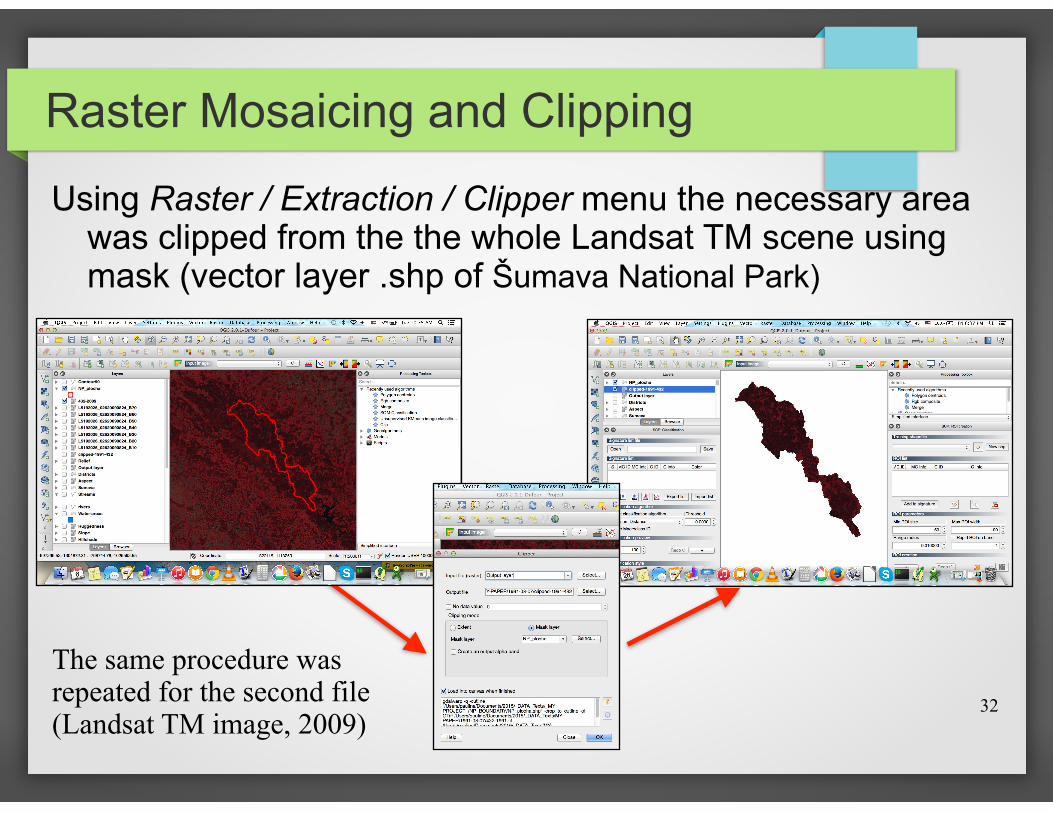
Raster Mosaicing and Clipping

Using Raster / Extraction / Clipper menu the necessary area was clipped from the the whole Landsat TM scene using mask (vector layer .shp of Šumava National Park)

The same procedure was repeated for the second file (Landsat TM image, 2009)

ClassificationThe Classification of the image has been performed using Semi - Automatic Classification Plugin The Classification Plugin allows supervised classification of Landsat TM images, providing tools to execute the classification process :

34

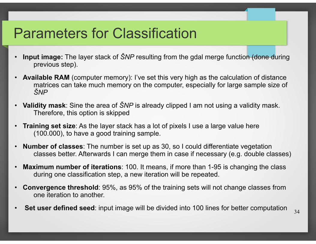
Parameters for Classification• Input image: The layer stack of ŠNP resulting from the gdal merge function (done during

previous step).

• Available RAM (computer memory): I’ve set this very high as the calculation of distance matrices can take much memory on the computer, especially for large sample size of ŠNP

• Validity mask: Sine the area of ŠNP is already clipped I am not using a validity mask. Therefore, this option is skipped

• Training set size: As the layer stack has a lot of pixels I use a large value here (100.000), to have a good training sample.

• Number of classes: The number is set up as 30, so I could differentiate vegetation classes better. Afterwards I can merge them in case if necessary (e.g. double classes)

• Maximum number of iterations: 100. It means, if more than 1-95 is changing the class during one classification step, a new iteration will be repeated.

• Convergence threshold: 95%, as 95% of the training sets will not change classes from one iteration to another.

• Set user defined seed: input image will be divided into 100 lines for better computation

35

Parameters for Classification: GUI of QGIS

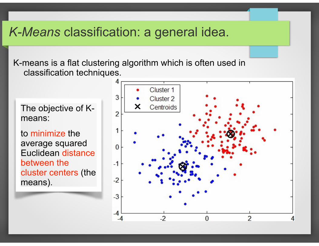
K-Means classification: a general idea.

K-means is a flat clustering algorithm which is often used in classification techniques.

The objective of K-means:

to minimize the average squared Euclidean distance between the cluster centers (the means).

The K-means analysis separates pixels into various clusters

by defining the mathematical centroids of all clusters

groups of pixel with similar values of spectral reflectance (digital number, DNs):

!!!!

K-Means clustering: a mathematical approach

The K-means separates raster pixels in n clusters (groups of equal variance) by minimizing the ‘inertia’ criterion.

Classification Output: 1991

Classification Results: Map of 1991

Classification Output: 2009

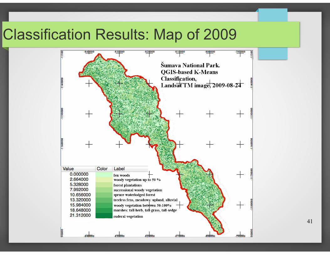
41

Classification Results: Map of 2009

Conclusions (I)Current research steps included… :

1. to collect, organize and sort data for research

2. to study, read and analyze relevant literature on research topic

3. to develop a tentative GIS method (algorithm) for producing spatio-temporal land cover maps for change detection analysis.

4. to receive preliminary results for available data (1991 and 2009)

Next steps will include…:

1) development of improved approach (comparison of various methods) discrimination of land cover types especially in the selected section of the study area, combine and compare the results from various algorithms with knowledge of vegetation and terrain characteristics

2) analyze any misclassification of forest areas (e.g. to reduce the problem of possible spectral confusion)

3) assessing and improving accuracy of both 1991 and 2009 images.

4) environmental analysis of “triggers-consequences”. For example, the depletion of certain land cover types can be attributed to environmental changes and (or) anthropogenic effects.

Conclusions (II)Methodologically, current research step also revealed the importance of spatial and

temporal remote sensing data and GIS tools for detecting changes of the environment

The importance of the GIS and remote sensing (RS) data were successfully used for the environmental monitoring since 1970s (rapid development of Earth observation satellite systems and launch of the Landsat TM program).

Therefore, the combination of remote sensing data and GIS tool for pattern recognition is proved to be effective tool for geo-botanical research

The spatial analysis performed by means of open source QuantumGIS enabled to use satellite images for geobotanical studies.

The spatio-temporal analysis was applied to Landsat TM images taken at 1991 and 2009. Built-in functions of the mathematical algorithms of QGIS enabled to process raster Landsat TM images and to derive information from them.

The classification of the images was used to analyze changes in the ŠNP area that consist in different geobotanical land cover types

The results of image processing demonstrate that structure, shape and configuration of landscapes in ŠNP changed since 1991

ReferencesBarešová M. and Hanusová Z. (2010). Zvláště chráněná území ČR - Národní parky - NP Šumava.

Online: http://www.kct-tabor.cz/gymta/ChranenaUzemiCR/SumavaNP/index.htm Bilek M., Kalal J., Bilek J. 1990. South Bohemia and Bohemian Forests information system (Spolek

pro popularizaci jižních Čech). Šumava. Online: http://www.jiznicechy.org/en/index.php?path=prir/npsumava.htm

Bláha J., Romportl D. and Křenová Z. (2013) Can Natura 2000 mapping be used to zone the Šumava National Park? European Journal of Environmental Sciences, Vol. 3 (1), pp. 57–64.

Bucharová A., Brabec J., Münzbergová Z. 2012. Effect of land use and climate change on the future fate of populations of an endemic species in central Europe. Biological Conservation 145, 39–47.

Chabera S. 1998. Fyzický zeměpis jižních Čech. Přehled geologie, geomorfologie, horopisu a vodopisu. Jihočeská univerzita, České Budějovice. 139 s.

Cudlinová E., Lapka M., Bartos M. 1999. Problems of agriculture and landscape management as perceived by farmers of the Šumava Mountains (Czech Republic). Landscape and Urban Planning 46, 71-82.

Ekrtová E., Kosnar J. 2012. Habitat-related variation in seedling recruitment of Gentiana pannonica. Acta Oecologica 45, 88-97. Hofhanzlova E., Fer T. 2009. Genetic variation and reproduction strategy of Gentiana pannonica in different habitats. Flora 204, 99–110.

Holubichková B., 1960: Studie o vegetaci blat. I. (Mrtvýluh) [A Study on the vegetation of moorlands I (“Mrtvýluh” in the Šumava Mountains)]. Sborník VŠZ, 1960, 129–149 (in Czech, English Summary).

References (continue)Jolecek M. et al. 1994. Ceska republika. Ucebnice zemepisu. Nakladatelstvi Ceske geograficke

spolecnosti. Janecková P., Wotavová K., Schodelbauerová I., Jersaková J., Kindlmann P. 2006. Relative effects

of management and environmental conditions on performance and survival of populations of a terrestrial orchid, Dactylorhiza majalis. Biological conservation 129, 40–49.

Křenová Z. and Hruska J. (2012) Proper zonation – an essential tool for the future conservation of the Šumava National Park. European Journal of Environmental Sciences, 62 (2), No 1.

Masková Z., Dolezal J., Kvet J., Zemek F. 2009. Long-term functioning of a species-rich mountain meadow under different management regimes. Agriculture, Ecosystems and Environment 132, 192–202.

Dickie I. and Whiteley G. (2013) An Outline of Economic Impacts of Management Options for Šumava National Park. Final Report. December 2013. The British Assessment Bureau, ISO 9001. Ochrana území. Online: http://www.npsumava.cz/cz/1016/sekce/ochrana-uzemi/

Prach K., Bufková I., Zemek F., Herman M., Masková Z. 2000. Grassland vegetation in the former military area Dobrá Voda, the Šumava National Park. Silva Gavreta 5, 101-112.

Schreiber H., 1924: Moore des Böhmerwaldes und des deutschen Südböhmen. IV. Sebastianberg, 119 pp.

Semotanová E. 1998. Historicka geografie Ceskych zemi. Historicky ustav, Praha, 293 s. Changes of plant species composition in the Šumava spruce forests, SW Bohemia, since the 1970s.

Final Slide

Thank you for attention. Questions ?