Environmental Regulation and Trade Openness in the Presence ofPrivate Mitigation1

Louis Hotte2 Stanley L. Winer3

August 31, 2010

1We thank Sophie Bernard, Cinzia Di Novi, Ruth Forsdyke, Michael Kevane, BryanPaterson, Stephane Straub and an anonymous referee for helpful comments. We alsothank seminar participants at CERDI-Universite d’Auvergne, Universite Paris 1 Pantheon-Sorbonne, the University of Ottawa, Universite de Rouen, the University of Western On-tario, the University of Eastern Piedmont, and participants in meetings of CSAE, the CEA,CREE and the IIPF, as well as the Montreal Natural Resources and Environmental Eco-nomics Workshop. Winer’s research was partly supported by the Canada Research ChairProgram. This work was also supported by a research grant from the SSHRCC.

2Department of Economics, University of Ottawa (louis.hotte@uottawa.ca)3School of Public Policy and Administration and Department of Economics, Carleton

University (stan winer@carleton.ca)

Abstract

Environmental Regulation and Trade Openness in the Presenceof Private Mitigation

Acknowledging the differential ability of individuals to privately mitigatethe consequences of pollution is essential for an understanding of demands forregulation of the environment and of trade in dirty goods, and for analysis ofthe implications of these demands for equilibrium policy choices. In a smallopen economy with exogenous policy, we first explain how private mitigationresults in an unequal distribution of the health consequences of pollution in amanner consistent with epidemiologic studies, and consequently how the ben-efits and costs of trade in dirty goods interact with choices concerning privatemitigation to polarize the interests of citizens concerning environmental strin-gency. The economy is then embedded in a broader political economy setting,and simulated to investigate the role of private mitigation in the determinationof policy choices. We show that when citizens can effectively choose betweencostly collective and costly private alternatives for pollution control, the samepolarization of interests underlies equilibrium policy choices concerning envi-ronmental regulation and trade openness in democratic and autocratic regimes.

Keywords: Environmental Regulation; Pollution; Private Mitigation; Trade,Dirty Goods; Individual Welfare; Health; Democracy; Representation Theorem.

JEL classification: D7, F18, Q56

1

1 Introduction

In this paper we analyze the demands by individuals of varying incomes for regulationof the environment and of trade, and the implications of these demands for equilibriumpublic policy choices. The economic setting is that of a small open economy producingtwo tradable goods, one of which is polluting, where more stringent environmentalcontrol reduces income. The differential ability of individuals to privately mitigatethe adverse consequences of pollution at a cost is a key characteristic of the analysisthroughout.

According to epidemiologic studies, the adverse health effects of pollution arenot equally distributed across the population; those with lower socioeconomic statustend to suffer a heavier health burden.1 For this reason, we might expect individualdemands for environmental regulation to be more intense among lower income groups.Similarly, when a country’s comparative advantage lies with the production of goodsthat are pollution-intensive, we might expect opposition to trade openness amonglower income citizens to be stronger .

On the other hand, it is often argued that environmental quality is a normal goodso that with diminishing marginal utility of consumption, richer individuals are willingto pay more for a cleaner environment. If that is the case, then poorer people willdemand laxer environmental regulation and more trade with specialisation in dirtyproduction. This is the basic reasoning behind Summers’ provocative 1991 memo atthe IMF, which put forward the idea that it may make sense for dirty industries tomove South.2

In the absence of private mitigation, there is certainly every reason to believe thatenvironmental quality is a normal good. But in the light of the epidemiologic studies,

1See, for instance, the empirical evidence in Ash and Fetter (2004), Pearce et al. (2006), Brooksand Sethi (1997), Neidell (2004), Jayachandran (2008) and Evans and Smith (2005) and the reviewsof Brunekreef and Holgate (2002) and O’neill et al. (2003). Moreover, news stories about how ittends to be the poorest within the developing countries who are affected by pollution are legion:see, for example, Bernard (2006), Bradsher and Barboza (2006), French (2005) or The Economist(2005).

2In the theoretical literature, Copeland and Taylor (1994) show that based on the normal-goodargument, a representative individual in a poor country optimally chooses lower environmentalstandards and thus specializes in dirtier industries. The assumption here is that all externalities aresomehow internalized. If that is not the case, and at the other end of this normative literature, arethe analyses of Pethig (1976) and Chichilnisky (1994) who take as given that environment standardsare lower in developing countries, and argue that although these countries (also) attract dirtierindustries, one cannot be sure that trade does not lower welfare; it depends on what drives thechoice of standards. On trade and endogenous internalization, see Copeland (2005) and Hotte, Longand Tian (2000). Finally, we note that while this normative literature informs our work, our concernis with positive aspects of how individual interests are shaped and how these demands play a rolein shaping equilibrium policy outcomes.

2

that this leads poorer individuals to always demand less stringent environmentalregulation and more open trade in domestically produced polluting goods does notseem sensible.3 Indeed, a similarly straightforward application of the normal goodargument also leads one to infer that wealthier individuals in developed countriesalways demand more restricted trade in polluting goods than do the poor.

In our view, it is not environmental quality per se which is a normal good. Rather,it is the health condition associated with it. Once this consideration is combinedwith the fact that the impact of pollution on health can be privately mitigated,there are far-reaching implications for our understanding of the relationships betweenenvironment regulation, trade openness and individual welfare.

We consider a small open economy with Ricardian production technology in whichindividuals differ a priori by income levels, along with its autarkic counterpart. Themodel is simplified so that closed-form derivation and comparison of economic equi-libria are possible. Here trade specialized in the polluting good versus autarky servesas a simplified policy option regarding the regulation of trade openness. The eco-nomic model (where policies are exogenously determined) allows for closed form inter-personal comparisons of the impact of environmental regulation even when pollutioncontrol interacts with the benefits of trade openness.4

The economy is then embedded in a broader political economy setting, and sim-ulated to further investigate the role of private mitigation in the determination ofpublic policy choices and their welfare consequences.

We show at the outset that in the economic framework we investigate, privatemitigation results in an unequal distribution of the health consequences of pollutionacross income groups in a manner consistent with epidemiologic studies, in contrast tomuch of the literature which assumes equal health effects for all.5 As a result, privatemitigation polarizes the interests of rich and poor with respect to the stringency ofregulation in a manner that we investigate in detail.

The interaction of private mitigation and trade openness exacerbates this diver-

3See Kahn and Matsusaka (1997) and Kristrom and Riera (1996) for some empirical evidence thatwithin a community or country, demand for environmental regulation may decrease with individualincome.

4The same qualitative effects would be present with the more general Heckscher-Ohlin frameworkbut this would come at a cost in terms of insight and clarity. As Feenstra (2004) points out, “... theRicardian model is as relevant today as it has always been.” (p. 1)

5 Analyses of the relationship between the environment and trade that assume equal healtheffects for all and which, one should note, are aimed at investigation of different issues than in thispaper, include Fredriksson (1997), Aidt (1998), Schleich (1999), McAusland (2003) and Copelandand Taylor (2003). An exception includes Copeland and Taylor (2003; §7.3) where it is assumed thatpeople’s tastes about the environment differ exogenously and without relation to income. Erikssonand Persson (2003) is the only study we have found where the negative effects of pollution decreasewith income. However, they assume that this happens exogenously and do not consider trade.

3

gence of interests. We show that when trade leads to a more polluted environmentcompared to autarky, the demand for publicly provided pollution control among high-income individuals may decrease. This is because the additional income that tradegenerates allows them to better insulated themselves from the heath consequences ofpollution. Moreover, since the gains from trade may be weaker for lower income in-dividuals, trade may lead to a strengthening of the poor’s demand for environmentalregulation. In such situations, a simple normal-good-based prediction will not serveas an accurate guide to the nature of individual interests in the open economy.6

It is reasonable to expect that the polarization of interests created by the interac-tion of private mitigation and trade will carry with it implications for the outcome ofpolitical competition. The basic reason is that introducing an ability to privately mit-igate alters individual incentives to seek costly collective as opposed to costly privateactions as a way of dealing with the health consequences of pollution. To study therole of private mitigation in a political context, we simulate the equilibrium relation-ship between environmental regulation, trade and welfare for two income groups infully democratic and in autocratic regimes differentiated by the presence or absenceof political voice for poorer citizens. The economic structure analyzed in the firstparts of the paper is embedded in the model used, and the role of private mitigationis studied by varying its effective cost.

We show that the costliness of private mitigation or, equivalently, the nature ofthe underlying pollutant, is a key factor underlying the equilibrium choice of policytowards the environment and towards trade. When private mitigation is infeasible,fully democratic and autocratic regimes in which the poor have no voice adopt thesame levels of regulation and of trade openness. But when mitigation is feasibleat some cost, the interests of the mass of poorer voters in dealing publicly withenvironmental degradation diverge from the those of the rich, and the outcome inthe fully democratic setting involves more regulation than in an autocracy. So theimportance of the interaction of private mitigation and trade openness uncoveredin the economic model with exogenous policy carries over to the equilibrium policycontext. Other authors - see, for example, Congleton 1992 and Winslow 2005 - arguethat democracy is good for the environment because elites have a greater share of anyincome generated by the production of dirty goods. Here we show why the cost ofprivate mitigation must also be acknowledged in the study of the political economyof environmental policy.7

6Note that, as discussed in footnote 23, our analysis does not contradict the EnvironmentalKuznets Curve hypothesis. For additional micro-economic perspectives on the demand for envi-ronmental regulation in the presence of private mitigation, see Coase (1960), Courant and Porter(1981), Shibata and Winrich (1983), Bartik (1988) and McKitrick and Collinge (2002).

7In a broader political economy context, we also indicate how cases may even arise where thepoor may oppose more trade openness in a democracy even though it has the potential to benefit

4

The paper is organized as follows. In section 2, we introduce the fundamental func-tions representing individual welfare as well as the production, regulation and privatepollution-mitigating technologies. We solve for decentralized consumption and pro-duction decisions in section 3. Those decisions are combined with the market-clearingconditions in section 4, for both autarky and for trade, and the resulting effects onpollution are derived in 5. In section 6 we compare the marginal welfare consequencesof environmental regulation for different income groups. We then describe, in section7, how trade openness may create conflicting demands for environmental regulation.In section 8, we introduce the political economy setting for the determination ofpolicy choices, which previously have been treated as exogenous, and we then ana-lyze political equilibria in several scenarios differentiated by the costliness of privatemitigation.

Section 9 concludes our analysis of the role of private mitigation in the relationshipbetween environmental policy, trade openness and economic well-being.

2 The economic model

2.1 Individual welfare

An individual i’s welfare level, denoted U(i), depends positively on his or her healthcondition, h(i), and the quantity of goods and services consumed, x(i). We furtherassume that the two are separable and exhibit decreasing marginal utility of con-sumption; that is,8

U(i) = u(x(i)) + h(i), ux > 0, uxx < 0.

In turn, the health condition depends negatively on the economy-wide pollutionlevel, denoted Q ≥ 0.9 This effect can, however, be privately mitigated with effortlevel d(i).10 Hence, h(i) = h(d(i), Q), hQ ≤ 0 and hd ≥ 0.

For tractability, we shall use the following functional forms in the ensuing anal-ysis: u(x(i)) = ln(x(i)) and h(i) = −[δ0 − δ1d(i)]Q, where parameter δ0 denotes

everyone, because of a concern that laxer environmental regulation with trade will then be imposedin the interests of richer citizens. Such a result is consistent with the shift of emphasis from anti-to alter-mondialisation among some (French and other) globalization protest movements. They donot oppose trade per se, but rather the type of trade that they observe.

8Unless otherwise noted, subscripts of functions denote partial derivatives.9Note that the analysis does not consider transboundary pollution issues such as greenhouse

gases.10Examples of pollution mitigation measures include choice of house location, installation of house-

hold water filtration system, drinking bottled water, fetching water at a distance, chlorine pills, aircleaning system, weekends at the mountain, asthma medicines, etc. See, for instance, Neidell (2004),Hanna (2007) and Rosado (2006).

5

the marginal effect of pollution on health in the absence of private mitigation andparameter δ1 summarizes the available private-mitigation technology. We thus have

U(i) = ln(x(i))− [δ0 − δ1d(i)]Q, d(i) ∈ (0, δ0/δ1). (1)

In the absence of pollution (Q = 0), or with maximum private mitigation (d(i) =δ0/δ1), i’s health condition attains its best state (h(i) = 0). Otherwise, if Q increaseswhile d(i) is fixed, the health condition worsens and the same holds if d(i) decreaseswhile Q is fixed. Because consumption exhibits decreasing marginal utility, the healthcondition is a normal good : a rise in income induces one to spend more on improvinghis health condition.11 A crucial feature of the model here is that there are twochannels through which an individual’s h(i) can increase: privately with higher d(i)or collectively with lower Q.

Note finally that as δ1 → 0, private mitigation becomes technologically impossible(or, equivalently, infinitely costly). In that case, with h(i) = δ0Q, the fact that healthis a normal good also makes environmental quality a normal good. This case willlater on serve as a benchmark that will be used to underscore and study the roleplayed by private mitigation.

2.2 The production technology

We assume an economy with two types of goods, denoted 1 and 2. Good 2 is a dirtygood in the sense that its production creates pollution while good 1 is clean and doesnot pollute at all. Production uses a Ricardian technology as represented by thefollowing (no-regulation) national production possibility frontier (PPF ):

Z2 = Z2 − bZ1, (2)

where Z2 and Z1 respectively denote the aggregate outputs of goods 2 and 1, pa-rameter b is the constant opportunity cost of producing an extra unit of good 1 interms of good 2, and Z2 measures the height of the PPF (an index of the country’stotal production capacity or wealth). With good 2 as the numeraire good and good1 selling at price p, the national income is

Y = pZ1 + Z2. (3)

2.3 Individual income

The economy is composed of a continuum of individual types indexed by i ∈ [0, 1] anddistributed according to density function f(i). The total population size is normalized

11This can be readily verified by solving the following problem: maxx,h u(x) + h s.t. y = x + ph,where y is income and p is the price of the health condition in units of the consumption goods.

6

to one. A priori, individuals differ solely by their claim on the national income, whichis expressed as the exogenous share α(i) > 0. Individual income is thus

y(i) = α(i)Y. (4)

Individuals are ranked so that α(i) is non-decreasing in i. Note that this represen-tation of heterogeneity allows us to concentrate on the divergent interests of citizensbased solely on income differences. Since relative factor endowments play no role, wedepart here from the manner in which the political-economic analysis of trade is ofteninvestigated. This is justified by the fact that individual interests in our frameworkdepend importantly on the ability to privately mitigate the effects of pollution, andthis ability is a function of income whatever its source.

2.4 Individual expenditures

Goods 1 and 2 are combined as imperfect substitutes for the creation of a finalgood C(i). We represent this by using the following Cobb-Douglas form: C(i) =C1(i)

aC2(i)1−a, where C1(i) and C2(i) respectively denote the quantities of goods 1

and 2 being combined. The unit cost of a final good is thus c(p) = a−a(1 − a)a−1pa

and we are left with the following budget constraint: y(i) = c(p)C(i). Final goodsare used either for consumption level x(i) or private pollution mitigation effort d(i)so that x(i) + d(i) = C(i).12

Let consumption expenditures be expressed as e(i) = c(p)x(i). The individualbudget constraint is then

e(i) = α(i)Y − c(p)d(i). (5)

2.5 Pollution and its regulation

In the absence of environmental regulation, the economy-wide pollution level Q issimply given by Q = Z2; that is, each unit of good 2 produces one unit of pollution.Environmental regulation requires the suppliers of good 2 to produce in a cleanerway. Some productive resources must be devoted to either cleaning up along theproduction process or using more sophisticated, cleaner production techniques. Eitherway, in comparison to the no-intervention case, environmental regulation has twodirect effects:

i) A benefit in the form of less pollution for any production level Z2;

12It should be noted that we are implicitly assuming that the consumption bundle and the pollutionmitigation effort bundle are equally pollution intensive. There is no a priori reason to believe thatpollution defensive measures are any more or any less pollution intensive than the mix of consumptiongoods on average.

7

ii) A cost in the form of more inputs necessary to achieve any production level Z2.

Let us define the stringency of environmental regulation as a continuous variableθ ∈ [0, 1]. θ = 0 imposes no restriction on emissions, while θ = 1 is an obligationto abate all emissions. Here there is no uncertainty surrounding the effectiveness ofenvironmental policy, and all pollution affects only the domestic environment.

The benefits and costs of regulation are represented as follows:

Benefit: Q = h(θ)Z2, with h′(θ) < 0, h(0) = 1 and h(1) = 0; (6)

Cost: Z2 = (1− θ)(Z2 − bZ1). (7)

It follows from from (7) that regulation results in a downward shift of the PPF : forany given amount of Zi, less of Zj is produced. Moreover, a pollution-free outputof good 2 is prohibitively costly. From a producer’s point of view, environmentalregulation simply increases the opportunity cost of producing the dirty good from1/b to 1/(1 − θ)b in terms of the clean goods. The maximum amount of the cleangood that can be produced is not affected by environmental regulation. We shallrefer to equation (7) as the regulated production possibility frontier (RPPF ) whichis illustrated in figure 1.

6

-Z1

Z2

a¦

b¦

Z2 = Z2 − bZ1

Z2 = (1− θ)(Z2 − bZ1)

9

Z1

Z2

(1− θ)Z2

Figure 1: The regulated production possibility frontier (RPPF)

8

3 Output and consumption decisions

We assume price-taking behavior throughout.

3.1 Production decisions

3.1.1 Autarky

Under the assumption of Ricardian technology, the opportunity cost of good 1 isconstant in terms of good 2 and equal to (1 − θ)b. Therefore, if both goods areproduced, we have pA = (1 − θ)b, where subscripts A denotes autarky. The autarkynational income is YA = (1− θ)bZ1 + Z2. Substituting the RPPF in (7), we obtain

YA = (1− θ)Z2. (8)

3.1.2 Trade

We consider the case of a small open economy. The world price of good 1 is fixed atpT , where subscript T denotes trade. There are two polar cases to consider:

(i) Specialization in the clean good

If pT ≥ (1− θ)b, only good 1 is produced and there is no pollution in equilibrium.Then national income is given by

YT = pTZ2

b. (9)

(ii) Specialization in the dirty good

If pT < (1− θ)b, only the dirty good is produced and there is pollution in equilib-rium. National income in this case is

YT = (1− θ)Z2. (10)

It is important to note that whether pT is larger or smaller than (1− θ)b dependson the stringency of environmental regulation.

3.2 Consumption decisions

With the assumed Cobb-Douglas forms for C(i), the quantities demanded for goods1 and 2 are, respectively, aα(i)Y/p and (1− a)α(i)Y .

We now have to solve for the allocation of expenditures between consumptiongoods (e(i)) and pollution mitigation (c(p)d(i)). To simplify, define v(p) ≡ 1/c(p)

9

and substitute x(i) = v(p)e(i) into the utility function so that the individual problemcan be expressed as follows:

max{e(i),d(i)}

V (i) = ln(v(p)e(i))− (δ0 − δ1d(i))Q (11)

s.t. e(i) = α(i)Y − c(p)d(i). (12)

The individual takes prices, pollution, environmental regulation and national in-come as given. Substituting e(i) in (11) for the budget constraint, the problem of anindividual reduces to choosing d(i). The first-order condition for an interior solutionis13

∂V (i)

∂d(i)= − c(p)

e∗(i)+ δ1Q = 0, (13)

where superscript ∗ denotes an individually optimal choice. This condition simplyequates the marginal welfare loss from a lower consumption level to the health gainfrom an increase in the pollution mitigation effort. Given that 0 ≤ d(i) ≤ δ0/δ1, weobtain the following interior and corner solutions:

d∗(i) = 0; e∗(i) = α(i)Y iff α(i) ≤ α, (14)

d∗(i) =δ0

δ1

; e∗(i) = α(i)Y − c(p) δ0δ1

iff α(i) ≥ α, (15)

d∗(i) =α(i)Y

c(p)− 1

δ1Q; e∗(i) = c(p)

δ1Qotherwise, (16)

where

α =c(p)

Y

1

δ1Q, (17)

α =c(p)

Y

[1

δ1Q+

δ0

δ1

]. (18)

According to corner solution (14), relatively poor individuals whose income sharelies below α choose not to spend anything on pollution mitigation because of theirhigh marginal utility of consumption. Conversely, solution (15) denotes relativelywealthy individuals with income shares above α who choose to be completely insulatedfrom the effects of pollution. Interior solution (16) represents intermediate-incomeindividuals who opt for a partial protection against pollution. Note how the pollution-mitigation effort tends to increase with the pollution level.

The welfare maximization solution allows us to assert the following:

Proposition 1 The individual pollution-mitigation effort (weakly) increases with pol-lution and with individual income. Consumption expenditure (weakly) decreases withpollution and (weakly) increases with individual income.

13It is straightforward to verify that the second-order conditions for a maximum are satisfied.

10

4 The general economic equilibrium

4.1 Equilibrium in autarky

In autarky, the supply of each good must be equal to its aggregate demand. We thushave

Z2A =

∫ 1

0

(1− a)YAα(i)f(i)di, (19)

= (1− a)(1− θ)Z2, (20)

where (20) is obtained using expression (8) for the national income. In autarky, givenθ, the economic general equilibrium is fully described by the following set of equations:

pA = (1− θ)b, (21)

Z2A = (1− a)YA, (22)

Z1A =aYA

p, (23)

QA = h(θ)Z2A, (24)

YA = (1− θ)Z2 (25)

and e∗(i) and d∗(i) are defined according to either of conditions (14), (15) or (16). Thesystem has 7 endogenous variables {pA, YA, Z1A, Z2A, QA, e∗(i), d∗(i)} and contains 7equations.

4.2 Equilibrium with trade

4.2.1 Specialization in the clean good

As shown in section 3.1.2, we have pT ≥ (1−θ)b. In the absence of pollution, we haved∗(i) = 0 and individual consumption spending is e(i) = α(i)YT = pT (α(i)Z2/b) (see(9)). In this case, consumers do not have any decision to make; they just spend alltheir income on consumption goods. Note that this is consistent with corner solution(14) when Q → 0.

As we have pointed out earlier, whether pT is larger or smaller than (1 − θ)bdepends on the stringency of environmental regulation. As a consequence, whetherthis outcome obtains or not hinges on the choice of θ, which ultimately depends on apolitical process (to be introduced later).

11

The general economic equilibrium with trade and specialization in the clean goodis summarized by the following system:

Z2T = 0, (26)

Z1T =Z2

b, (27)

e∗(i) = α(i)YT , (28)

d∗(i) = 0, (29)

QT = 0, (30)

YT =pT

bZ2 (31)

4.2.2 Specialization in the dirty good

We now have pT < (1− θ)b and the country produces only good 2. There is pollutionin this trade equilibrium, which is summarized by the following system:

Z1T = 0, (32)

Z2T = (1− θ)Z2, (33)

QT = h(θ)Z2T , (34)

YT = (1− θ)Z2 (35)

with e∗(i) and d∗(i) being determined according to either of conditions (14), (15) or(16). Since the price is now exogenous, the economic system now has 6 endogenousvariables {YT , Z1T , Z2T , QT , e∗(i), d∗(i)} and 6 equations as well.

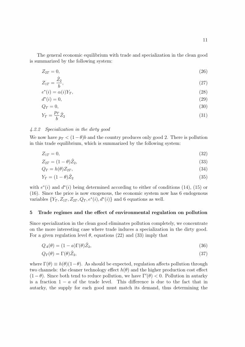
5 Trade regimes and the effect of environmental regulation on pollution

Since specialization in the clean good eliminates pollution completely, we concentrateon the more interesting case where trade induces a specialization in the dirty good.For a given regulation level θ, equations (22) and (33) imply that

QA(θ) = (1− a)Γ(θ)Z2, (36)

QT (θ) = Γ(θ)Z2, (37)

where Γ(θ) ≡ h(θ)(1−θ). As should be expected, regulation affects pollution throughtwo channels: the cleaner technology effect h(θ) and the higher production cost effect(1− θ). Since both tend to reduce pollution, we have Γ′(θ) < 0. Pollution in autarkyis a fraction 1 − a of the trade level. This difference is due to the fact that inautarky, the supply for each good must match its demand, thus determining the

12

relative output proportions between the clean and dirty goods. With trade, however,demand and supply are disjoint. In the case of a Ricardian production technology,full specialization in the production of the dirty good 2 results in a jump in pollution.This leads us to assert the following:14

Proposition 2 Compared to autarky, an increase in pollution regulation stringencyhas a larger pollution-reducing impact when the country is open to trade and specializedin the dirty good. More precisely, the impact of a change in the degree of pollutioncontrol in autarky is equal to a fraction 1− a of that with trade.

and

Proposition 3 Compared to autarky and for a fixed regulation level, trade with spe-cialization in the dirty good induces individuals to (weakly) increase their pollution-mitigation effort.

6 The welfare effects of environmental regulation

We now wish to analyze how an exogenous increase in the stringency of environmentalregulation affects individual welfare in the general-equilibrium setting. (In the caseof trade, we do so while assuming specialization in the dirty good only.) To this end,we make use of the following indirect utility function which can be obtained by directsubstitution of the results in (14), (15) and (16):

= ln(v(p)α(i)Y )− δ0Q iff α(i) ≤ α,

V ∗(p, y(i), Q) = ln

(v(p)α(i)Y − δ0

δ1

)iff α(i) ≥ α, (38)

= ln

(1

δ1Q

)−

[δ0 − δ1

(α(i)Y

c(p)− 1

δ1Q

)]Q otherwise.

In general, we have that:

d

dθV ∗(p, y(i), Q) =

[∂V ∗(i)

∂pp′(θ) +

∂V ∗(i)∂y

α(i)Y ′(θ)]

︸ ︷︷ ︸price-income effect

+

[∂V ∗(i)

∂QQ′(θ)

]

︸ ︷︷ ︸pollution effect

(39)

The impact of regulation on individual welfare reveals itself through prices, incomeand pollution. To gain insight, we analyze the price-income effect, represented by the

14Proofs of propositions are found in the Appendix.

13

first term between square brackets, separately from the pollution effect, given by thesecond term between square brackets.15 In the economic equilibrium, we have

p′A(θ) = −b in autarky and p′T (θ) = 0 with trade, (40)

Y ′A(θ) = Y ′

T (θ) = −Z2, (41)

Q′A(θ) = (1− a)Γ′(θ)Z2 and Q′

T (θ) = Γ′(θ)Z2. (42)

In autarky and for trade with specialization in the dirty good, these conditions yield

= −νk

{[1

1− θ

]+

[δ0Γ

′(θ)Z2

]}iff α(i) ≤ αk,

d

dθV ∗

k (i) = −νk

[α(i)Z2

e∗k(i)

]iff α(i) ≥ αk, (43)

= −νk

{[α(i)Z2

e∗k(i)

]+

[(δ0 − δ1d

∗k(i))Γ

′(θ)Z2

]}otherwise,

where k ∈ {A, T}, νA = 1−a and νT = 1. In each case, the first term between squarebrackets denotes the price-income effect while the second one – when present – isthe pollution effect. For α(i) ≥ αk, the pollution effect is absent since those highestincome individuals are completely insulated from pollution. We begin by analyzingthe pollution effects.

6.1 The pollution welfare effects of regulation

We have the following:

Proposition 4 In both trade and autarky, the marginal pollution welfare gains froma more stringent pollution regulation (weakly) decrease with individual income shareα(i).

The intuition behind this result is that richer individuals tend to be better insulatedfrom the effects of pollution because of their mitigation efforts.

We now want to compare the importance of the pollution welfare effects of regu-lation when moving from autarky to trade. In this respect, two opposite effects arise.One the one hand, there is a higher pollution reduction effect with trade than au-tarky (proposition 2). On the other hand, individuals tend to (weakly) increase theirprivate-mitigation effort with trade (proposition 3). We thus obtain the followingresult:

15We expect that this approach will also be useful for the conduct of empirical work.

14

Proposition 5 The pollution welfare effect of regulation is strictly more importantwith trade than autarky for individuals whose income share is below some unique valueα, while it is (weakly) less important for all the other, richer individuals.

This is a key result because it informs us about how the economic equilibriumstructures a divergence of interests among citizens. Whether the economy is openedto trade or not, the poorest segment of the population remains highly exposed to pol-lution. These people choose not to privately mitigate because of the high marginalutility of their consumption. Then given that trade causes more pollution, regulat-ing pollution must have a stronger beneficial effect on their health with trade thanautarky. For richer individuals, recall that by increasing real income and pollution,trade induces them to mitigate further. For those who receive a large enough shareof aggregate income, the increased mitigation effort is so large that they become lesssensitive to a reduction in pollution. Figure 2 summarizes proposition 5.

α(i)-

−δ0Γ′(θ)Z2

αA αAαT

−δ0(1− a)Γ′(θ)Z2

αT

6pollutioneffect

α

trade

autarkyδ1 = 0

δ1 > 0

Figure 2: The marginal pollution welfare effect of regulation by income share forautarky and trade

6.2 The price-income welfare effects of regulation

In order to have a complete picture of the welfare effects of regulation, we mustalso consider the price-income effect. To do so, we can begin with the followingproposition:

15

Proposition 6 The marginal price-income effect of regulation varies non-monotonicallywith income shares. In absolute terms, it is (weakly) increasing at low income shares(below α) and decreasing at high income shares (above α).

The best way to understand this result is by first observing that in the absence ofprivate mitigation possibilities, the marginal price-income effect is the same regardlessof income share. Indeed, even though those with higher income shares lose more fromregulation in absolute terms, they also have a lower marginal utility of income, andthe logarithmic form of utility that we use causes both effects to cancel out exactly.But once we introduce private mitigation possibilities, the diversion of expendituresaway from consumption increases the marginal utility of income, so that there is nowa net loss. The non-monotonicity stems from the fact that the poorest segment of thepopulation does not privately mitigate while for the very rich, private mitigation haslittle effect on their consumption. Hence, for these two extreme income share levels,the marginal price-income effect converges to the same value, as if private mitigationpossibilities were absent.

We also can assert the following:

Proposition 7 In absolute terms, the marginal price-income effect of regulation ismore important with trade than autarky for all income shares below or equal to αT ,as well as for arbitrarily large income shares.

The basic intuition here is that with specialisation in the production of the dirtygood, regulating pollution is more costly with trade than autarky. There is onepossible exception for the income shares around αA. The ambiguity is caused by thefact that αT < αA and that the marginal price-income effect is decreasing under tradefor α(i) > αT while in autarky, it increases up to αA.

Figure 3 illustrates propositions 6 and 7 for both trade and autarky.

7 Trade regimes and the demand for environmental regulation

We now analyze how trade openness affects the aggregate demand for environmentalregulation. In this section, we continue to take the regulation level as given andconsider the marginal effect of regulation on welfare when moving from autarky totrade. In the following section, we shall compare welfare levels when the degree ofregulation emerges from a political process.

Note that in the analysis of individual demands for regulation, we shall considerboth the number of individuals who demand stricter or laxer regulation and also vari-ations in the intensity or depth of individual demands. Both numbers and intensityof demands play a role in the political process. We first have the following result:

16

-α(i)

1−a1−θ

11−θ

αT αA αT αA

6price-income

effect

trade

autarky

δ1 = 0

δ1 > 0

Figure 3: The marginal price-income welfare effect of regulation by income share forautarky and trade

Proposition 8 The proportion of individuals who demand more environmental reg-ulation is lower with trade than autarky.

This proposition may appear counter-intuitive. Even though trade results in amore polluted environment, some individuals who in autarky preferred more stringentregulation now prefer less. But recall that the generation of more pollution constitutesonly one channel through which trade affects the demand for regulation. One mustalso consider the price-income effect and the change in the pollution-mitigation effortthat occur.

Under the assumptions of our model, the shift of expenditures from consumptionto private mitigation induced by the higher pollution associated with open tradealong with income gains makes individuals in the interior solution for d∗A(i) moresensitive to the price-income losses from regulation in comparison to the gains fromlower pollution. This is illustrated in figure 4, where it is assumed that the followinginequality holds: 1/(1−θ) < −δ0Q

′T (θ).16 The figure combines both the pollution and

price-income marginal effects of figures 2 and 3. In autarky, the indifferent individualwho receives income share αA of the national income is (locally) indifferent betweenmore or less regulation as his price-income loss is exactly compensated by his pollutiongain. Under trade, his pollution gain falls while the price-income loss increases, andhe now prefers strictly lower regulation. Under trade, the indifferent individual is onewho receives a strictly lower income share αT .

16This inequality insures that in autarky, the lowest income individuals would prefer to have morestringent regulation. Given the previous results, this preference will become even more intense withtrade.

17

6

α(i)-

11−θ

−δ0Γ′(θ)Z2

αA αAαT

−δ0(1− a)Γ′(θ)Z2

1−a1−θ

price-income loss

pollution gain

autarky

autarky

trade

trade

αT αT αA

Figure 4: Pollution and price-income effects by income shares, for autarky and trade

One may be tempted to infer from the above that open trade leads to less stringentregulation. But this assumes that government policy is driven by numbers of votersonly. A more complete view will account for changes in the intensity of preferences.In this respect, we have the following two propositions:

Proposition 9 For lower income individuals, the intensity of the demand for morestringent pollution regulation increases with trade.

This is illustrated in figure 4 by the fact that the gap between the pollution gainfrom more regulation and the price-income loss grows larger the lower the incomeshare of an individual.

Proposition 10 For high-income individuals and for a range of intermediate incomelevels, the intensity of the demand for less stringent pollution regulation increases withtrade.

For instance, in figure 4, one sees that those with high enough income will losemore from additional regulation under trade than under autarky.

We therefore have that on the one hand, trade reduces the number of peopledemanding more regulation (proposition 8). On the other hand, trade increases the

18

intensity of the demand for more stringent regulation by the poorest individuals(propositions 9), while simultaneously increasing the intensity of the demand forless stringent regulation by the richest individuals, as well as for some intermediateincome levels (proposition 10). These effects are not revealed by a simple normalgood argument about environmental quality. Moreover, if regulation is a result ofa political process that responds to the demands of citizens, then merely looking atchanges at the number of individuals who demand more regulation may not suffice.One must also account for individual sensitivities to regulation.

In this respect, we are left with an indeterminacy concerning the impact of tradeon the stringency of environmental regulation that is adopted. The policy outcomewill depend on how the political process effectively weighs the heterogeneous andconflicting demands of various voters.17 What we can say at this point is the following,which derives directly from propositions 9 and 10:

Proposition 11 Trade exacerbates the divergence of interests over environmentalregulation between low and high income individuals.

In this section, we analyzed the effects of marginal variations in environmentalregulation on individual welfare. We decomposed the marginal welfare effects ofregulation into its various sub-components. This procedure yields insight into how thepossibility of private mitigation, interacting with trade openness, leads to divergenceof interests in environmental regulation when policy choices are exogenous. In thenext section we depart from the marginal analysis of the effects of given policy choicesand broaden the framework of analysis to include the determination of policy and thelevel of welfare in a political equilibrium.

8 The political-economy of environmental regulation in the presence ofprivate mitigation

We proceed by simulating equilibria in political settings in which the economic struc-ture analyzed above is embedded. To bring out the role of private mitigation, we firstconsider equilibria in which the possibility of mitigation is absent or prohibitivelyexpensive for everyone, and then compare these outcomes to those that emerge whenmitigation is feasible at some cost.

Our principal interest is in the role of mitigation in a fully democratic, competitiveprocess. As is well-known, the outcome of such a political process can be representedby maximization, over the set of available policy instruments, of a synthetic functionS that is a weighted sum of individual (indirect) utilities of the poor V ∗

P and of the

17This is consistent with the recent empirical evidence in Farzin and Bond (2006) and Dasguptaet al. (2006).

19

rich V ∗R (see for example, Coughlin and Nitzan 1981, Coughlin 1992, and Hettich and

Winer 1999):

S = sηP V ∗P + (1− s)ηRV ∗

R (44)

Here the economic structure outlined earlier has been substituted into the indirectutility functions. Maximization of (44) is carried out with respect to the degree ofenvironmental regulation θ, which is a continuous policy choice, and trade openness,which in our framework is a discrete choice. To simplify, but in a manner that allowsthe previous analysis to be used, all individuals have been aggregated into two groups,poor (P ) and rich (R), with population weights s and (1− s). The use of two incomegroups is sufficient to bring out the importance of the role of private mitigation.18

The weights ηP and ηR reflect the effective political influence of the representativemember of each group. These weights need not be identical in a democracy, but weshall assume that they are, further strengthening our focus on the role of privatemitigation.19

It is important to note that the form of the support function in (44) and the weightson utilities are the result of the political process, and that the support function isnot a social welfare function. The maximization problem in (44) is just a convenientway of calculating an equilibrium. The intuition behind the representation theoremis this: if a political party in a competitive, democratic system does not proposeor implement platforms that move the society towards the Pareto frontier, it leavesopen the possibility that the opposition can improve the welfare of voters and therebyincrease its chances of electoral success. Competition insures that no such policymoves remain in equilibrium.20

To proceed further, we assume the following functional form for the effect ofenvironmental regulation on pollution:

h(θ) = 1− θ. (45)

We also need to choose parameters for the economic structure, to be held constantthroughout. The following values are ones that we have found to produce simulationsthat are especially illuminating:

b = 1, Z2 = 3, a = 0.5, δ0 = 2, pT = 0.1.

18The use of two income groups is a simplification that has been used in many other politicaleconomy investigations, such as that by Acemoglu and Robinson (2006).

19On the difference between economic interests and political influence, see Hotte and Winer (2001).20While policy choices are efficient in this formulation, the representation theorem can be gener-

alized to allow for inefficient policy by breaking the link between utility and voting behavior (see,for example, Hettich and Winer 1999, ch. 6). We are not concerned with these inefficiencies here.

20−

4−

20

0 .2 .4 .6 .8 1Pollution regulation

AutarkyTrade

Welfare of the poor

−2

02

0 .2 .4 .6 .8 1Pollution regulation

Welfare of the rich

−4

−2

0

0 .2 .4 .6 .8 1Pollution regulation

S

Figure 5: The welfare of the poor and the rich in autarky and trade, autocracy anddemocracy without private mitigation technology (δ1 = 0)

Finally, to set up the simulations, the poor and the rich respectively are assumedto make up 95% and 5% of the total population, the total size of which is normalizedto one, with the income share of a rich individual set at eleven times that of a poorone, that is, αR = 11αP .

8.1 Equilibria without private mitigation

We begin the simulations with the case in which private mitigation is impossible foranyone, that is, when δ1 = 0. The resulting zero mitigation equilibria are illustratedin figure 5. The first panel shows the welfare of the poor in autarky and in the openeconomy, the second panel shows the welfare of the rich or equivalently, the welfareof the elite in the autocratic regime, again in autarky and under trade. Panel threeshows political support S in (44), the maximization of which can be used to modelthe democratic outcome.

To help in understanding the shape of the curves in figure 5, we note first thatin the absence of private mitigation, both groups prefer autarky over trade whenthe regulation level is low. This is because trade gains then cannot make up for thehealth losses that come with full specialisation in the production of the dirty good.We note also that when θ ≥ 0.9, political support in a democracy, illustrated in thethird panel, is constant under trade. This is because at θ = 0.9 there is a completeshift of specialisation in the economy from the dirty good to the clean good, and so

21

any further increase in regulation has no consequence for the welfare of voters.Globally speaking, the interests of the poor and the rich are perfectly aligned in

the absence or infeasibility of private mitigation. Both groups globally prefer opentrade with a substantial pollution regulation level set at θ = 0.7.21 Since both groupshave the same interests with respect to public policy, autocracy and democracy leadto the same equilibrium policy choices.

Proposition 12 In the absence of private mitigation, the political equilibria are iden-tical under both democracy and autocracy, and both groups gain from trade.

8.2 Equilibria when private mitigation is feasible

Things are quite different when private mitigation is feasible at a cost, as illustratedby the simulations with δ1 = 0.2 shown in figure 6. The interests of the rich andthe poor are still perfectly aligned in autarky as in figure 5 (at point b in panel 1and at e in panel 2). However, for the rich we see that the best option is for theeconomy to be opened to trade, and that trade openness be combined with the lowestregulation level in order to attain the highest welfare (at point a in panel 2). Thehigher pollution levels from specialisation that accompanies trade, combined with thehigher income this produces, induce the rich to spend so much on private mitigationthat they are insulated from the effects of pollution, and they would then prefer toreduce the regulation level to its minimum in order to benefit fully from trade gains.22

Such an outcome turns out to be the worst for the poor who cannot afford to protectthemselves (see point d in panel 1). Thus when private mitigation is feasible, it turnsout that in the simulations of political equilibria, as in the marginal economic analysisearlier, trade openness interacts with choices about private mitigation to polarize theinterests of citizens.

How are these interests represented in the political equilibrium of autocracy andof the democratic state? We see from figure 6 that trade openness is chosen underboth political regimes, because both the welfare of the rich (in the case of autocracy)and political support (in the democratic case) are highest then. But environmentalregulation levels are different in these two regimes.

In the open economy, an autocratic regime controlled by a rich elite would reducethe regulation level to zero, making the rest of the population worse-off than under

21This welfare maximizing value for θ is approximate since we simulated the economy with discreteincrements of θ of 0.05.

22On the other hand, panel 2 indicates that with trade openness and increasingly strict regulation,the rich eventually will choose not to privately mitigate anymore, if given the choice, because of theconsequent fall in their income and in the level of pollution, and they thus would return to publicregulation as a preferred choice for dealing with pollution. This explains the presence of two localwelfare maxima for the rich illustrated in the second panel of figure 6.

22

b

d

c

−4

−2

0

0 .2 .4 .6 .8 1Pollution regulation

AutarkyTrade

Welfare of the poor

e

a

−2

02

0 .2 .4 .6 .8 1Pollution regulation

Welfare of the rich

−4

−2

0

0 .2 .4 .6 .8 1Pollution regulation

S

Figure 6: The welfare of the poor and the rich in autarky and trade, autocracy anddemocracy with private mitigation (δ1 = 0.2)

autarky (compare points b and d in panel 1 of figure 6). In this sense, trade andthe feasibility of private mitigation together bring out the worst aspects of the non-democratic regime. In the democratic case, or speaking more generally, when lowerincome voters exercise political voice, the interests of the mass of voters swamp thatof the rich. A stricter equilibrium regulation level of θ = 0.7 (that maximizes S in thethird panel of figure 6) emerges. In that case, collective choice leads to public actionconcerning environmental externalites because most voters cannot mitigate privately.

These patterns lead us to offer a final proposition and corollary about the rela-tionship between environmental regulation and democracy:

Proposition 13 (’Democracy is good for environmental protection’) When the healthconsequences of pollution can be mitigated privately at a cost, the nature of the politicalregime matters for the nature of equilibrium policy. In small open economies, publicregulation of pollution will be stricter in democracies than in autocracies or in regimesgoverned by elites.

The corollary is that when private mitigation is feasible, poorer citizens lose fromtrade in non-democratic regimes, while they gain from trade in a fully competitive,democratic system. In contrast, the rich gain from trade regardless of the regimetype.

23

In assessing these results, it is important to recall that when private mitigationis infeasible, environmental regulation in the equilibria of both democratic and non-democratic regimes is the same. So in the present framework, it is not simply the factthat the poor have voice in a democracy that distinguishes them. The interaction ofthe cost of private mitigation and the consequences of trade in determining the leveland distribution of economic welfare is also crucial.

As we noted in the introduction, both Congleton (1992) and Winslow (2005) ar-gue that pollution control is greater in democracies because elites in non-democraticregimes receive a larger share of the income produced by the expansion of dirty in-dustries, as they do in our framework. They also provide some empirical evidence tothis effect. Proposition 13 and its corollary point also to the critical role of privatemitigation in the relationship between the type of regime and the nature of environ-mental control, the cost of which will vary for different types of pollution, and whichis not acknowledged in these interesting studies.

8.3 Intensity of preferences and the democratic equilibrium

In a last simulation, we illustrate our assertion that when it comes to trade andpollution in the presence of private mitigation, the intensity of preferences for regu-lation along with the size of interest groups is likely to play a role in determining theoutcome of the democratic process.

In our representation of democratic political equilibria, the government maximizesa particular weighted sum of utilities S in (44). The effect of a change in regulationon optimized political support is therefore given by

∆S

∆θ= s

∆V ∗P

∆θ+ (1− s)

∆V ∗R

∆θ. (46)

Here, population numbers interact multiplicatively with the sensitivities of welfare tochanges in environmental controls - in other words, with the intensity of preferencesfor regulation - to determine which way the policy equilibrium will change.23

According to Proposition 11, trade exacerbates the divergence of interests betweenthe poor and the rich. In expression (46), this translates into situations in which, forexample, trade increases ∆V ∗

P /∆θ and reduces ∆V ∗R/∆θ. Figure 7 illustrates such a

case. The only change from the situation illustrated in figure 6 is that the privatemitigation technology parameter is raised from 0.2 to 0.4. This change - which reduces

23 Note that we do not deal here with how pollution control and pollution vary with mean in-come levels, which is the subject of the Environmental Kuznets Curve (EKC), and our results arenot inconsistent with it. Recent empirical results suggest that the EKC is driven mostly by howgovernance correlates with mean income (see, for example, Torras and Boyce (1998), Fredriksson etal. (2005), Farzin and Bond (2006) and Dasgupta et al. (2006)).

24−

4−

20

0 .2 .4 .6 .8 1Pollution regulation

AutarkyTrade

Welfare of the poor

−2

02

0 .2 .4 .6 .8 1Pollution regulation

Welfare of the rich

−4

−2

0

0 .2 .4 .6 .8 1Pollution regulation

S

Figure 7: The role of the intensity of preferences (δ1 = 0.4)

the effective cost of private mitigation - has little impact on the decisions of the poorabout mitigation. But it is enough of a change to induce the rich to be well protectedprivately against the health effects of pollution in autarky when the level of publicregulation level is low.

As a consequence, the rich now prefer that there be no public regulation at all,either with or without trade, while the poor still want some positive level of publicpollution control. And in line with proposition 11, this divergence of interests isexacerbated by a move to open trade. We see in figure 7 that as regulation increases,the welfare of the rich drops more sharply under trade than under autarky, while thewelfare of the poor increases more sharply.

Due to their larger number, the democratic equilibrium under trade still favorsthe poor, at s = 0.95. But the fact remains that with trade, the absolute loss for therich from stricter regulation is larger than in the closed economy. So while the richmay not mind so much about stricter environmental regulation under autarky, theymay not be so pliable in an open economy. This observation suggests that (in a morecomplicated political setting than we have simulated) the rich may bargain harderbefore accepting stricter environmental regulation when their welfare is relativelymore sensitive to policy changes. And if commitment to policy is a problem from theperspective of the poor, one can envisage situations in which the poor vote againstmore open trade even though it has the potential to improve the welfare of everyone,because they fear that more lax regulation will then be introduced in the interests of

25

the rich.It is interesting to point here to a comparison with Verdier’s (2004) work on trade

integration. He argues that since trade openness affects a government’s ability toredistribute, it is not possible to discuss the politics of globalization without alsoconsidering those of internal redistribution. In this paper, the ability to redistributeis not explicitly part of the analysis. But in the analysis and simulations we haveconducted, trade does raise the need for compensation of the poor due to the healtheffects of the pollution generated, depending on the costliness of private mitigation,and in a democratic equilibrium the rich essentially make sacrifices in their favor.In other words, when trade leads to environmental degradation, it is important tojointly analyze the distributive consequences of trade openness and of environmentalregulation, and to do so in the presence of private mitigation, in order to understandpublic policy in either dimension.

9 Conclusion

We have analyzed in detail how the nature and heterogeneity of demands for publicregulation of environmental externalities among citizens of differing incomes dependon the cost of private mitigation. And we have shown how the study of public policytowards regulation of the environment and of trade in dirty goods is altered whenindividual citizens can choose between costly collective and costly private alternativesfor pollution control.

To better isolate the role of private mitigation, we have broken the link betweenfactor endowments and citizen interests employed in much of the existing literature ontrade and pollution, because private mitigation depends solely on individual incomeregardless of its source. In the context of a small open economy, we then analyzed indetail how the benefits and costs of open trade in dirty goods interacts with choicesconcerning private mitigation to polarize the interests of citizens concerning the de-gree of environmental regulation. Even though trade openness leads to increasedpollution, the possibility of using some of the extra income generated by trade forprivate mitigation may allow the wealthiest to actually shelter themselves so as tobe less affected by pollution. Poorer individuals may not be in a position to affordsuch protection even after benefitting from the gains that open trade produces, andwill tend to favor collective rather than private action. In addition, we have analyzedhow the intensity, as well as the direction, of individual demands for environmentalregulation is affected by the possibility of private mitigation.

It follows from this analysis that the demands for trade openness are heteroge-neous with respect to direction and intensity, and are also importantly influenced bythe possibility of private mitigation. For it matters what kind of trade, with whatdegree of pollution regulation, one considers when analyzing who is in favor and who

26

is against more openness. It is not surprising, therefore, that introducing the abilityto privately mitigate at a cost opens up a host of possibilities concerning the na-ture of environmental regulation and its relationship to trade openness in a politicalequilibrium.

We conclude that acknowledging the role of private mitigation is essential for afull understanding of the political economy of the environment - trade - welfare nexus.

APPENDIX

Proof of proposition 2: It derives directly from equations (36) and (37).

Proof of proposition 3: Note first that with specialization in the dirty good, we haveYT = YA. Given θ, trade causes both an increase in pollution Q and a decreasein the unit cost c(p) of the pollution-mitigating effort. From (16), this results ina higher interior d∗(i). As for corner solutions (14) and (15), it can be readily veri-fied from (17) and (18) that trade’s higher Q and lower c(p) reduces α and increases α.

Proof of proposition 4: In the case of corner solutions, the marginal pollution effectis independent of α(i). In the interior solution, the marginal pollution effect is equalto −(δ0 − δ1d

∗k(i))Q

′k(θ). The result follows from the fact that d∗k(i) is increasing in

α(i), ∀k ∈ {A, T}.

Proof of proposition 5: The proof proceeds from the fact that the marginal pollutioneffect curve is continuous and non-increasing in α(i), as per proposition 4. The ideais then to show that the trade curve is steeper than the autarky one, that it beginsabove it and ends below it.

(a) Since αT < αA, all individuals with α(i) ≤ αT choose d∗(i) = 0, whether withtrade or autarky. For them, the marginal pollution effect is equal to −δ0(1−a)Γ′(θ)Z2

in autarky and −δ0Γ′(θ)Z2 with trade (see (43)). Hence, the marginal pollution effect

curve under trade is strictly above that of autarky at low α(i).(b) For those who choose to be completely insulated from the effects of pollution,

the marginal pollution effect is at the minimum value of zero. Since αT < αA, themarginal pollution effect is zero under trade for all α(i) ≥ αT , while it is strictlypositive under autarky for all α(i) ∈ (αT , αA). This implies that at αT , the marginalpollution effect under trade is strictly below that of autarky and that for all α(i) ≥ αT ,the curve under autarky is not below the trade curve.

(c) For α(i) ≤ αT , the slope is zero for both trade and autarky. For α(i) ∈(αT , αT ), the slope under trade is strictly negative while it is either zero or strictlynegative under autarky. Now the strictly negative slopes correspond to the interior

27

value for d∗k(i) and are given by the following (see (43)):

∂

∂α(i)

{−νk

[(δ0 − δ1d

∗k(i))Γ

′(θ)Z2

]}= νk

[δ1Γ

′(θ)Z2

] ∂

∂α(i)d∗k(i), k ∈ {A, T}.

According to (16), we have

∂

∂α(i)d∗k(i) =

Yk

c(pk)

Since YA = YT = (1− θ)Z2, c(pA) > c(pT ) and νA < νT , we have that the (negative)slope is steeper with trade than autarky.

Proof of proposition 6: The marginal price-income effects of regulation are given bythe first terms between square brackets in (43) for all income shares. Taking thederivatives with respect to α(i) yields the following:

∂

∂α(i)

[νk

1

1− θ

]= 0 when α(i) ≤ αk,

∂

∂α(i)

[νk

α(i)Z2

α(i)Y − c(p) δ0δ1

]< 0 when α(i) ≥ αk, (47)

∂

∂α(i)

[νk

α(i)Z2

c(p)δ1Q

]> 0 when αk < α(i) < αk.

Hence, the marginal price-income effect is initially constants up to α(i) = αk, is in-creasing for αk < α(i) < αk and is decreasing for α(i) ≥ αk. The proof is completeby noting that the marginal effect is continuous at both αk and αk, which can beverified by substituting the values in (17) and (18).

Proof of proposition 7: The marginal price-income effects of regulation are given bythe first terms between square brackets in (43) for all income shares. For α(i) ∈ [0, αT ],the result is obtained by substituting for νA = 1 − a and νT = 1, and for e∗A(i) ande∗T (i) in (14) and (16). For α(i) > αA, one can verify that limα(i)→∞ dV ∗

k (i)/dθ =−νk/(1− θ), ∀k ∈ {A, T}. The result follows from the fact that νT > νA.

Proof of proposition 8: Let αk denote the wealth level of an individual who ismarginally indifferent between more or less regulation, given θ. From (43), it canbe verified that αk, if it exists, is unique and must be in an interior solution withrespect to the pollution-mitigation effort. Moreover, αk necessarily exists if there are

28

some individuals who would prefer strictly more environmental regulation. αk mustbe such that the price-income and pollution effects are equal; that is,

αZ2

e∗k(i)= (δ0 − δ1d

∗k(i))Γ

′(θ)Z2. (48)

From (16), we have that e∗A(i) > e∗T (i) and d∗A(i) < d∗T (i). Hence, the LHS of (48) ishigher with trade than autarky while the converse holds for the RHS. An indifferentindividual in autarky will see his price-income effect of regulation strictly exceed thepollution effect with trade and specialization in the dirty good. The proof is madecomplete by the fact that the price-income effect increases with α(i) while the oppo-site holds for the pollution effect.

Proof of proposition 9: For all those whose pollution mitigating-effort is nil with trade,the gap between the marginal pollution effect and the marginal price-income effect ishigher by a factor 1/(1 − a) when opening up to trade; their demand for additionalregulation is thus more intense with trade. Among those who protect themselves par-tially, we have determined that income share αT denotes the marginally indifferentindividuals with trade and that the same individuals demanded strictly more regula-tion in autarky; the intensity of their demand for additional regulation has decreasedwith trade. By continuity of both marginal effect curves, an income share must existwhich is comprised strictly between αT and αT and for which the intensity of thedemand for additional regulation is equal in both autarky and trade.

Proof of proposition 10: Concerning the wealthiest individuals, we have seen thatfor arbitrarily large income shares, the pollution effect is nil while the price-incomeeffect increases with trade (proposition 7). Concerning intermediate income shares,it can be verified that although the price-income effect of regulation peaks at αk inboth trade and autarky, its magnitudes is higher with trade than autarky. Hence, bycontinuity of the curves, individuals with income shares located next to αk on bothsides are more severely and negatively affected by regulation with trade than autarky.

29

References

Acemoglu, Daron, and James S. Robinson (2006) Economic Origins of Dictatorshipand Democracy (Cambridge University Press)

Aidt, Toke S. (1998) ‘Political internalization of economic externalities and environ-mental policy.’ Journal of Public Economics 69, 1–16

Ash, M., and T.R. Fetter (2004) ‘Who lives on the wrong side of the environmentaltracks? Evidence from the EPA’s risk-screening environmental indicator model.’Social Science Quarterly 85, 441–462

Bartik, Timothy J. (1988) ‘Evaluating the benefits of non-marginal reductions inpollution using information on defensive expenditures.’ Journal of EnvironmentalEconomics and Management 15, 111–27

Bernard, Philippe (2006) ‘La rage d’Esperance Edoukou, victime des dechets toxiquesdeverses a Abidjan.’ Le Monde 13.09.06

Bradsher, Keith, and David Barbosa (2006) ‘Pollution from chinese coal casts a globalshadow.’ The New York Times 11.06.06

Brooks, Nancy, and Rajiv Sethi (1997) ‘The distribution of pollution: Communitycharacteristics and exposure to air toxics.’ Journal of Environmental Economicsand Management 32, 233–250

Brunekreef, B., and S.T. Holgate (2002) ‘Air pollution and health.’ The Lancet360, 1233–42

Chichilnisky, Graciela (1994) ‘North-south trade and the global environment.’ TheAmerican Economic Review 84(4), 851–874

Coase, R. H. (1960) ‘The problem of social cost.’ The Journal of Law and EconomicsIII, 1–44

Congleton, Roger D. (1992) ‘Political institutions and pollution control.’ The Reviewof Economics and Statistics 74, 412–421

Copeland, B.R., and M.S. Taylor (1994) ‘North-south trade and the environment.’Quarterly Journal of Economics 109, 755–87

(2003) Trade and the Environment: Theory and Evidence (Princeton, USA andOxford, UK: Princeton University Press)

30

Copeland, Brian R. (2005) ‘Policy endogeneity and the effects of trade on the envi-ronment.’ Agricultural and Resource Economics Review 34, 1–15

Coughlin, Peter J. (1992) Probabilistic Voting Theory (Cambridge University Press)

Coughlin, Peter J., and Shmuel Nitzan (1981) ‘Electoral outcomes with probabilisticvoting and nash social welfare maxima.’ Journal of Public Economics 15(1), 113–21

Courant, Paul N., and Richard C. Porter (1981) ‘Averting expenditure and the costof pollution.’ Journal of Environmental Economics and Management 8, 321–29

Dasgupta, S., K. Hamilton, K. Pandey, and D. Wheeler (2006) ‘Environment dur-ing growth: Accounting for governance and vulnerability.’ World Development34, 1597–1611

Eriksson, Clas, and Joakim Persson (2003) ‘Economic growth, inequality, democrati-zation, and the environment.’ Environmental and Resource Economics 25, 1–16

Evans, Mary F., and V. Kerry Smith (2005) ‘Do new health conditions supportmortality-air pollution effects?’ Journal of Environmental Economics and Man-agement 50, 496–518

Farzin, Y.Hossein, and Craig A. Bond (2006) ‘Democracy and environmental qual-ity.’ Journal of Development Economics 81, 213–235. Paper presented at the2005 Canadian Resource and Environmental Economics Annual Meeting, HECMontreal

Feenstra, Robert C. (2004) Advanced International Trade: Theory and Evidence(Princeton University Press)

Fredriksson, Per G. (1997) ‘The political economy of pollution taxes in a small openeconomy.’ Journal of Environmental Economics and Management 33, 44–58

Fredriksson, Per G., Eric Neumayer, Richard Damania, and Scott Gates (2005) ‘Envi-ronmentalism, democracy, and pollution conrol.’ Journal of Environmental Eco-nomics and Management 49, 343–365

French, Howard W. (2005) ‘Riots in Shanghai suburb as pollution protest heats up.’The New York Times 19.07.05

Hanna, Brid Gleeson (2007) ‘House values, incomes, and industrial pollution.’ Journalof Environmental Economics and Management 54, 100–112

31

Hettich, Walter, and Stanley L. Winer (1999) Democratic Choice and Taxation: ATheoretical and Empirical Analysis (New York: Cambridge University Press)

Hotte, Louis, and Stanley L. Winer (2001) ‘Political influence, economic interestsand endogenous tax structure in a Computable Equilibrium framework: Withapplication to the united states, 1973 and 1983.’ Public Choice 109, 69 – 99

Hotte, Louis, Ngo Van Long, and Huilan Tian (2000) ‘International trade with en-dogenous enforcement of property rights.’ Journal of Development Economics62, 25–54

Jayachandran, Seema (2008) ‘Air quality and early-life mortality: Evidence from In-donesia’s wildfires.’ NBER Working Papers 14011, National Bureau of EconomicResearch, Inc, May

Kahn, Matthew E., and John G. Matsusaka (1997) ‘Demand for environmental goods:Evidence from voting patterns on California inititives.’ Journal of Law and Eco-nomics XL, 137–173

Kristrom, Bengt, and Pere Riera (1996) ‘Is the income elasticity of environmentalimprovements less than one?’ Environmental and Resource Economics 7(1), 45–55

McAusland, Carol (2003) ‘Voting for pollution policy: The importance of incomeinequality and openness to trade.’ Journal of International Economics 61, 425–451

McKitrick, Ross, and Robert A. Collinge (2002) ‘The existence and uniqueness ofoptimal pollution policy in the presence of victim defense measures.’ Journal ofEnvironmental Economics and Management 44, 106–122

Mining in Peru: Halting the rush against gold (2005) The Economist

Neidell, Matthew J. (2004) ‘Air pollution, health, and socio-economic status: Theeffect of outdoor air quality on childhood asthma.’ Journal of Health Economics23, 1209–1236

O’neill, Marie S., and Al. (2003) ‘Health, wealth, and air pollution: Advancing theoryand methods.’ Environmental Health Perspectives 111, 1861–1870

Pearce, J., S. Kingham, and P. Zawar-Reza (2006) ‘Every breath you take? environ-mental justice and air pollution in Christchurch, new zealand.’ Environment andPlanning A 38, 919–938

32

Pethig, R. (1976) ‘Pollution, welfare, and environmental policy in the theory ofcomparative advantage.’ Journal of Environmental Economics and Management2, 160–169

Rosado, Marcia A. et Al. (2006) ‘Combining averting behavior and contingent valu-ation data: An application to drinking water treatment in Brazil.’ Environmentand Development Economics 11, 729–746

Schleich, Joachim (1999) ‘Environmental quality with endogenous domestic and tradepolicies.’ European Journal of Political Economy 15, 53–71

Shibata, Hirofumi, and J. Steven Winrich (1983) ‘Control of pollution when theoffended defend themselves.’ Economica 50, 425–437

Torras, Mariano, and James K. Boyce (1998) ‘Income, inequality, and pollution: Areassessment of the environmental Kuznets curve.’ Ecological Economics 25, 147–160

Verdier, Thierry (2004) ‘Socially responsible trade integration: A political economyperspective.’ Discussion Paper Series 4699, CEPR

Winslow, Margrethe (2005) ‘Is democracy good for the environment?’ Journal ofEnvironmental Planning and Management 48, 771–783