environmental regulations, air and water pollution, and
TRANSCRIPT

Massachusetts Institute of Technology Department of Economics
Working Paper Series
Environmental Regulations, Air and Water Pollution, and Infant Mortality in India
Michael Greenstone
Rema Hanna
Working Paper 11-11 July 1, 2011
Revised: February 18, 2013
Room E52-251 50 Memorial Drive
Cambridge, MA 02142
This paper can be downloaded without charge from the Social Science Research Network Paper Collection at
http://ssrn.com/abstract=1907924

Environmental Regulations, Air and Water Pollution, and Infant Mortality in India*
Michael Greenstone, MIT and NBER
Rema Hanna, Harvard Kennedy School, NBER and BREAD
February 2013
Abstract Using the most comprehensive data file ever compiled on air pollution, water pollution, and environmental regulations from a developing country, the paper examines the effectiveness of India’s environmental regulations. The air pollution regulations were responsible for substantial improvements in air quality. The most successful air regulation resulted in a modest, but statistically insignificant decline in infant mortality. The water regulations had no measurable benefits. Qualitative and quantitative evidence suggests that higher relative demand for air quality prompted the effective enforcement of air pollution regulations, indicating that environmental regulation can succeed in weak institutional settings when there is strong public support. JEL Codes: H2, Q5, Q2, O1, R5 Keywords: Air pollution; Water pollution; Benefits of environmental regulations; India
* Greenstone: MIT Department of Economics, E52-359, 50 Memorial Drive, Cambridge, MA 02142-1347 (e-mail: [email protected]) Hanna: Harvard Kennedy School, 79 JFK Street (Mailbox 26), Cambridge, MA 02138 and National Bureau of Economic Research, Bureau for Research and Economic Analysis of Development (e-mail: [email protected]). We thank Samuel Stolper, Jonathan Petkun, and Tom Zimmermann for truly outstanding research assistance. In addition, we thank Joseph Shapiro and Abigail Friedman for excellent research assistance. Funding from the MIT Energy Initiative is gratefully acknowledged. The analysis was conducted while Hanna was a fellow at the Science Sustainability Program at Harvard University. The research reported in this paper was not the result of a for-pay consulting relationship. Further, neither of the authors nor their respective institutions have a financial interest in the topic of the paper that might constitute a conflict of interest.

I. Introduction
Weak institutions are a key impediment to advances in well being in many developing
countries. Indeed, an extensive literature has documented many instances of failed policy in
these settings and has been unable to identify a consistent set of ingredients necessary for policy
success (Banerjee, Glennerster and Duflo, 2008; Duflo et al., 2012; Banerjee, Hanna and
Mullainathan, forthcoming). The specific question of how to design effective environmental
regulations in developing countries with weak institutions is increasingly important for at least
two reasons.1
India provides a compelling setting to explore the efficacy of environmental regulations
for several reasons. First, India's population of nearly 1.2 billion accounts for about 17 percent
of the world’s population. Second, it has been experiencing rapid economic growth of about 6.4
percent annually over the last two decades, placing significant pressure on the environment. For
example, Figure 1, Panel A demonstrates that ambient particulate matter concentrations in India
are five times the United States level (while China's are seven times the U.S. level) in the most
recent years with comparable data, while Figure 1, Panel B shows that water pollution
concentrations in India are also higher. Further, a recent study concluded that India currently has
the worst air pollution out of the 132 countries analyzed (Environmental Performance Index,
2013). Third, India is widely regarded as havingsub-optimal regulatory institutions: Identifying
which regulatory approaches succeed in this context would be of great practical value. More
First, "local" pollutant concentrations are exceedingly high in many developing
countries and in many instances are increasing (Alpert et al., 2012). Further, the high pollution
concentrations impose substantial health costs, including shortened lives (Chen, et al., 2013;
Cropper, 2010; Cropper, et al., 2012), so understanding the most efficient ways to reduce local
pollution could significantly improve wellbeing. Second, the Copenhagen Accord makes it clear
that it is up to individual countries to devise and enforce the regulations necessary to achieve
their national commitments to combat global warming by reducing greenhouse gas emissions
(GHG). Since most of the growth in GHG emissions is projected to occur in developing
countries, such as India and China, the planet's wellbeing rests on the ability of these countries to
successfully enact and enforce environmental policies.
1 There is a large literature measuring the impact of environmental regulations on air quality, with most of the research focused on the United States. See, for example, Chay and Greenstone (2003 and 2005), Greenstone (2003), Greenstone (2004), Henderson (1996), and Hanna and Oliva (2010), etc. The institutional differences between the United States and many developing countries mean that the findings are unlikely to be valid for predicting the impacts of environmental regulations in developing countries.
2
generally, since the air and water regulations were implemented and enforced in different
manners, a comparison of their relative effectiveness can shed light on how to design policy
successfully in weaker regulatory contexts. Fourth, India has a rich history of environmental
regulations that dates back to the 1970s, providing a rare opportunity to answer these questions
with extensive panel data.2
This paper presents a systematic evaluation of India’s environmental regulations with a
new city-level panel data file for the years 1986-2007 that we constructed from data on air
pollution, water pollution, environmental regulations, and infant mortality. The air pollution data
comprise about 140 cities, while the water pollution data covers 424 cities (162 rivers). Neither
the government nor other researchers have assembled a city-level panel database of India's anti-
pollution laws, and we are unaware of a comparable data set in any other developing country.
We consider two key air pollution policies, the Supreme Court Action Plans and the
Mandated Catalytic Converters, as well as India’s primary water policy, the National River
Conservation Plan, which focused on reducing industrial pollution in rivers and creating sewage
treatment facilities.3
The analysis indicates that environmental policies can be effective in settings with weak
regulatory institutions. However, the effect is not uniform, as we find a large impact of the air
pollution regulations, but no effect of the water pollution regulations. In the preferred
econometric specification that controls for city fixed effects, year fixed effects and differential
pre-existing trends among adopting cities, the requirement that new automobiles have catalytic
converters is associated with large reductions in airborne particulate matter with diameter less
than 100 micrometres (µm) (PM) and sulfur dioxide (SO2) of 19 percent and 69 percent,
respectively, five years after its implementation. Likewise, the Supreme Court-mandated Action
Plans are associated with a decline in nitrogen dioxide (NO2) concentrations; however, these
policies are not associated with changes in SO2 or PM. In contrast, the National River
These regulations resemble environmental legislation in the United States
and Europe, thereby providing a comparison of the efficacy of similar regulations across very
different institutional settings.
2 Previous papers have compiled data sets for a cross-section of cities or a panel for one or two cities, including Foster and Kumar (2008; 2009), which examines the effect of CNG policy in Delhi; Takeuchi, Cropper, and Bento (2007), which studies automobile policies in Mumbai; Davis (2008), which looks at driving restrictions in Mexico; and Hanna and Oliva (2011), which studies a refinery closure in Mexico City. 3 We also documented other anti-pollution efforts (e.g., Problem Area Action Plans, and the sulfur requirements for fuel), but they had insufficient variation in their implementation across cities and/or time to allow for a credible evaluation.
3
Conservation Plan—the cornerstone water policy—was not associated with improvements in the
three available measures of water quality.
As a complement to these results, we adapt a Quandt likelihood ratio test (Quandt, 1960)
from the time-series econometrics literature to the difference-in-differences (DD) style setting to
probe the validity of the findings. Specifically, we test for a structural break in the difference
between adopting and non-adopting cities’ pollution concentrations and assess whether the
structural break occurs around the year of policy adoption. The analysis finds evidence of a
structural break in adopting cities’ PM and SO2 concentrations around the year of adoption of the
catalytic converter policy and no breaks in the time-series that correspond to cities’ adoption of
the National River Conservation Plan. In addition to these substantive findings, this
demonstrates the value of this technique in DD style settings.
We conclude that the striking difference in the effectiveness of the air and water pollution
regulations reflects a greater demand for air quality by India's citizens. This conclusion is based
on a mix of qualitative and quantitative evidence. Higher demand for clean air is to be expected
given the international evidence that ambient air quality is responsible for an order of magnitude
greater number of premature fatalities than water pollution. Moreover, the costs of self-
protection against air pollution are substantially higher than against water pollution; household
technologies to clean dirty water and bottled water are effective and inexpensive, while
comparable technologies for protection against air pollution simply do not exist. Additionally,
higher demand for clean air is consistent with the greater public discourse on air quality: We
find that the Times of India, the country’s leading English-language newspaper, reports on air
pollution three times as much as water pollution. Further, high levels of citizen engagement
caused India’s Supreme Court, widely considered the country's most effective public institution,
to promptly promulgate many air pollution regulations and follow up on their enforcement. In
contrast, the water regulations were characterized by jurisdictional opacity about
implementation, enforcement that was delegated to agencies with poor track records, and a
failure to identify a dedicated source of funds. These differences in promulgation and
enforcement are especially striking because there are many similarities between the legislations
that govern air and water pollution regulation.
Empirical evidence supports these qualitative findings. We assess whether the
effectiveness of air pollution regulations differed with observed proxies for the demand for clean

4
air. We find that the catalytic converter policies were more effective in cities with greater
newspaper attention to the problems of air pollution and in cities with higher education levels. In
contrast, measured corruption levels, which should not be related to the relative demand for clean
air, are not systematically associated with differences in the effectiveness of the catalytic
converter policy across cities.
Finally, we tested whether the catalytic converter policy, which had significant effects on
air pollution, was associated with changes in measures of infant health. To the best of our
knowledge, this is the first paper to relate infant mortality rates to environmental regulations in a
developing country context.4
The paper proceeds as follows. Section II provides a brief history of environmental
regulation in India focusing on the policies that the paper analyzes. Section III describes the data
sources and presents summary statistics on the city-level trends in pollution, infant mortality, and
adoption of environmental policies in India. Section IV outlines the econometric approach and
Section V reports and discusses the results. Section VI presents evidence that the relative success
of the air regulations reflected a greater demand for air quality improvements. Section VII
concludes.
The data indicate that a city’s adoption of the policy is associated
with a decline in infant mortality, but this relationship is not statistically significant. As we
discuss below, there are several reasons to interpret the infant mortality results cautiously.
II. Background on India’s Environmental Regulations
India has a relatively extensive set of regulations designed to improve both air and water
quality. Its environmental policies have their roots in the Water Act of 1974 and Air Act of
1981. These acts created the Central Pollution Control Board (CPCB) and the State Pollution
Control Boards (SPCBs), which are responsible for data collection and policy enforcement, and
also developed detailed procedures for environmental compliance. Following the
implementation of these acts, the CPCB and SPCBs quickly advanced a national environmental
monitoring program (responsible for the rich data underlying our analysis). The Ministry of
Environment and Forests (MoEF), created in its initial form in 1980, was established largely to
set the overall policies that the CPCB and SPCBs were to enforce (Hadden, 1987). 4 See Chay and Greenstone (2003) for the relationship between infant mortality and the Clean Air Act in the United States. Burgess, Deschenes, Donaldson, and Greenstone (2011) estimate the relationship between weather extremes and infant mortality rates using the same infant mortality data used in this paper.

5
The Bhopal Disaster of 1984 represented a turning point in India’s environmental policy.
The government’s treatment of victims of the Union Carbide plant explosion “led to a re-
evaluation of the environmental protection system,” with increased participation of activist
groups, public interest lawyers, and the judiciary (Meagher, 1990). In particular, there was a
steep rise in public interest litigation, and the Supreme Court instigated a wide expansion of
fundamental rights of citizens (Cha, 2005). These developments led to some of India's first
concrete environmental regulations, such as the closures of limestone quarries and tanneries in
Uttar Pradesh in 1985 and 1987, respectively.5
Throughout the 1980s and 1990s, India continued to adopt policies that were designed to
counteract growing environmental damage. The paper’s empirical focus is on two key air
pollution policies, the Supreme Court Action Plans (SCAPs) and the catalytic converter
requirements, and the primary water pollution policy, the National River Conservation Plan.
These policies were at the forefront of India’s environmental efforts. Importantly, there was
substantial variation across cities in the timing of adoption, which provides the basis for the
paper’s research design.
We discuss the Supreme Court's role in the
promulgation and enforcement of air pollution regulations in greater detail in Section VI.
The first policy we focus on is the Supreme Court Action Plans. The Action Plans are
part of a broad, ongoing effort to stem the tide of rising pollution in cities identified by the
Supreme Court of India as critically polluted. The SCAPs involve the implementation of a suite
of policies that could include fuel regulations, building of new roads that bypass heavily
populated areas, transitioning of buses to CNG, and restrictions on industrial pollution.
Measured pollution concentrations are a key ingredient in the determination of these
designations. In 1996, Delhi was the first city ordered to develop an action plan, while the most
recent action plans were mandated in 2003.6
Although the exact form of the SCAPs varies across cities, they are typically aimed at
reducing several types of air pollutants. At least one round of plans was directed at cities with
To date, 17 cities have been given orders to
develop action plans.
5 See Rural Litigation and Entitlement Kendra v. State of Uttar Pradesh (Writ Petitions Nos. 8209 and 8821 of 1983), and M.C. Mehta v. Union of India (WP 3727/1985). 6 As documented in the court orders, the Supreme Court ordered nine more action plans in critically polluted cities “as per CPCB data” after Delhi. A year later, the Court chose four more cities based on their having pollution levels at least as high as Delhi’s. Finally, a year later, nine more cities (some repeats) were identified based on Respired Suspended Particulate Matter (i.e., smaller diameter particulate matter) concentrations.

6
unacceptable levels of Respired Suspended Particulate Matter (RSPM), which is a subset of PM
characterized by the particles’ especially small size. Given the heavy focus on vehicular
pollution, it is reasonable to presume that the plans affected NO2 levels. Finally, since SO2 is
frequently a co-pollutant, it may be reasonable to expect the Action Plans to affect its ambient
concentrations. However, there has not been a systematic exploration of the SCAP’s
effectiveness across cities.7
The second policy we examine is the mandatory use of catalytic converters for specific
categories of vehicles, which was a policy distinct from the SCAPs. The fitment of catalytic
converters is a common means of reducing vehicular pollution across the world, due to the low
cost of its end-of-the-pipe technology. In 1995, the Supreme Court required that all new petrol-
fueled cars in the four major metros (i.e., Delhi, Mumbai, Kolkata, and Chennai) were to be
fitted with converters. In 1998, the policy was extended to 45 other cities. It is plausible that
this regulation could affect all three of our air quality indicators.
Just as with the SCAPs, there has not been a systematic evaluation of the catalytic
converter policies. Qualitative evidence suggests that the catalytic converter policies were
enforced stringently by tying vehicle registrations to installation of a catalytic converter.8
Finally, we study the cornerstone of efforts to improve water quality, the National River
However, it is not clear that this was indeed successful: Oliva (2011), Davis (2008), and
Bertrand et al. (2007) all show that drivers often evade regulations. Moreover, in contrast to the
SCAPs, public response to the catalytic converter policy was less favorable for several reasons:
Petrol’s lower fuel share made the scope of the policy narrower than, for example, the mandate
for low-sulfur in diesel fuel; unleaded fuel, which is necessary for effective functioning of
catalytic converters was at best inconsistently available until 2000; and the implementation in
only a subset of cities created opportunities for purchases of cars in the uncovered cities that
would be driven in the covered cities.
7 Many believe that the overwhelming approval of Delhi’s CNG bus program as part of its Action Plan provides indications of its success. Takeuchi, Cropper, and Bento (2007) show that the imposition of a similar conversion of buses to CNG would be the most effective policy for reducing passenger vehicle emissions in Mumbai. 8 Narain and Bell (2005) write, “In 1995 the Delhi government announced that it would subsidize the installation of catalytic converters in all two- and three-wheel vehicles to the extent of 1,000 Rs. within the next three years (Indian Express, January 30, 1995). Furthermore, the Petroleum Ministry banned the registration of new four-wheel cars and vehicles without catalytic converters in Delhi, Mumbai, Chennai, and Calcutta effective April 1, 1995 (Telegraph, March 13, 1995). This directive was implemented, although it is alleged that some vehicle owners had the converters removed illegally (court order, February 14, 1996).”
7
Conservation Plan (NRCP). Begun in 1985 under the name Ganga Action Plan (Phase I), the
water pollution control program expanded first to tributaries of the Ganga River, including the
Yamuna, Damodar, and Gomti in 1993. It was later extended in 1995 to the other regulated
rivers under the new name of NRCP. Today, 164 cities on 35 rivers are covered by the NRCP.
The criteria for coverage by the NRCP are vague at best, but many documents on the plan cite
the CPCB Official Water Quality Criteria, which include standards for BOD, DO, FColi, and pH
measurements in surface water. Much of the focus has centered on domestic pollution control
initiatives over the years (Asian Development Bank, 2007). The centerpiece of the plan is the
Sewage Treatment Plant: The interception, diversion, and treatment of sewage through piping
infrastructure and treatment plant construction has been coupled with installation of community
toilets, crematoria, and public awareness campaigns to curtail domestic pollution. If the policy
has been effective, it should affect several forms of water pollution; but the largest impacts
would be expected to be on FColi levels, which are most directly related to domestic pollution.
The NRCP has been panned in the media for a variety of reasons, including poor
cooperation among participating agencies, imbalanced and inadequate funding of sites, and an
inability to keep pace with the growth of sewage output in India’s cities (Suresh et al., 2007, p.
2). However, similar to the air pollution programs, there has never been a systematic evaluation
or even a compilation of the data that would allow for one.
III. Data Sources and Summary Statistics
To conduct the analysis, we compiled the most comprehensive city-level panel data file
ever assembled on air pollution concentrations, water pollution concentrations, and
environmental policies in any developing country. We supplemented this data file with a city-
level panel data file on infant mortality rates. This section describes each data source and
presents some summary statistics, including an analysis of the trends in the key variables.
A. Regulation Data
India has implemented a series of environmental initiatives over the last two decades.
Using multiple sources, we assembled a dataset that systematically documents these policy
changes at the city-year level. We utilized print and web documents from the Indian
government, including the CPCB, the Department of Road Transport and Highways, the
Ministry of Environment and Forests, and several Indian SPCBs. We then exploited information
8
from secondary sources, including the World Bank, the Emission Controls Manufacturers
Association, and Urbanrail.net. We believe that a comparable data set does not exist for India.
Table 1 summarizes the prevalence of these policies in the data file of city-level air and
water pollution concentrations by year. Columns (1a) and (2a) report the number of cities with
air and water pollution readings, respectively. The remaining columns detail the number of these
cities where each of the studied policies is in force. The subsequent analysis exploits the
variation in the year of enactment of these policies across cities.9
B. Pollution Data
Air Pollution Data. This paper takes advantage of an extensive and growing network of
environmental monitoring stations across India. Starting in 1987, India’s Central Pollution
Control Board (CPCB) began compiling readings of NO2, SO2, and PM. The data were collected
as a part of the National Air Quality Monitoring Program, which was established by the CPCB to
identify, assess, and prioritize the pollution control needs in different areas, as well as to aid in
the identification and regulation of potential hazards and pollution sources.10 Individual State
Pollution Control Boards (SPCBs) are responsible for collecting the pollution readings and
providing them to the CPCB for checking, compilation, and analysis. The air quality data are
collected from a combination of CPCB online and print materials for the years 1987-2007.11
The full dataset includes 572 air pollution monitors in 140 cities. Many of these monitors
operate for just a subset of the sample, and for most cities data is not available for all years.
12 In
the earliest year (1987), the functioning monitors cover 20 cities, while 125 cities are monitored
by 2007 (see Appendix Table 2 for annual summary statistics). On average, there are 2.3
monitors per city, with 78 percent of cities possessing data from more than one monitor in a
given year.13
The monitored pollutants can be attributed to a variety of sources. PM is regarded by the
Figure 2 maps cities with air pollution data in at least one year.
9 Appendix Table 1 replicates Table 1 for all cities in India. 10 For a more detailed description of the data, see http://www.cpcb.nic.in/air.php (accessed on June 25, 2011). 11 From the CPCB, we obtained monthly pollution readings per city from 1987-2004, and yearly pollution readings from 2005-2007. The monthly data were averaged to get annual measures. 12 The CPCB requires that 24-hour samplings be collected bi-weekly from each monitor for a total of 104 observations per monitor per year. As this goal is not always achieved, 16 or more successful hours of monitoring are considered representative of a given day’s air quality, and 50 days of monitoring in a year are viewed as sufficient for data analysis. Some cities, such as Delhi, conduct more frequent readings, but we do not include these. 13 Each monitor is classified as belonging to one of three types of areas: residential (71 percent), industrial (26 percent), or sensitive (2 percent). The rationale for specific locations of monitors is, unfortunately, not known to us at this time so all monitors with sufficient readings are included in the analysis.

9
CPCB as a general indicator of pollution, receiving key contributions from “fossil fuel burning,
industrial processes and vehicular exhaust”. SO2 emissions, on the other hand, are
predominantly a byproduct of thermal power generation; globally, 80 percent of sulfur emissions
in 1990 were attributable to fossil fuel use (Smith, Pitcher and Wigley, 2001). NO2 is viewed by
the CPCB as an indicator of vehicular pollution, though it is produced in almost all combustion
reactions.
Water Pollution Data. The CPCB also administers water quality monitoring, in
cooperation with SPCBs. As of 2008, 1,019 monitoring stations are maintained under the
National Water Monitoring Programme (NWMP), covering rivers and creeks, lakes and ponds,
drains and canals, and groundwater sources. We focus on rivers due to the consistent availability
of river quality data, the seriousness of pollution problems along the rivers, and, most
significantly, the attention that rivers have received from public policy. We have obtained from
the CPCB, in electronic format, observations from 489 monitors in 424 cities along 162 rivers
between the years 1986 and 2005 (see Appendix Table 2).14
The CPCB collects either monthly or quarterly river data on 28 measures of water
quality, of which nine are classified as “core parameters”. We focus on three core parameters:
Biochemical Oxygen Demand (BOD), Dissolved Oxygen (DO), and Fecal Coliforms (FColi).
We chose them because of their presence in CPCB Official Water Quality Criteria, their
continual citation in planning and commentary, and the consistency of their reporting.
Figure 3 maps the locations of these
monitors along India’s major rivers.
15
These indicators can be summarized as follows. BOD is a commonly-used broad
indicator of water quality that measures the quantity of oxygen required by the decomposition of
organic waste in water. High values are indicative of heavy pollution; however, since water-
borne pollutants can be inorganic as well, BOD is not considered a comprehensive measure of
water purity. DO is similar to BOD except that it is inversely proportional to pollution; that is,
lower quantities of dissolved oxygen in water suggest greater pollution because water-borne
waste hinders mixing of water with the surrounding air, as well as hampering oxygen production
from aquatic plant photosynthesis.
Finally, FColi, is a count of the most probable number of coliform bacteria per 100 14 From 1986 to 2004, monthly data is available. For 2005, the data is only available yearly. 15 See Water Quality: Criteria and Goals (February 2002); Status of Water Quality in India (April 2006); and the official CPCB website, http://www.cpcb.nic.in/Water_Quality_Criteria.php.
10
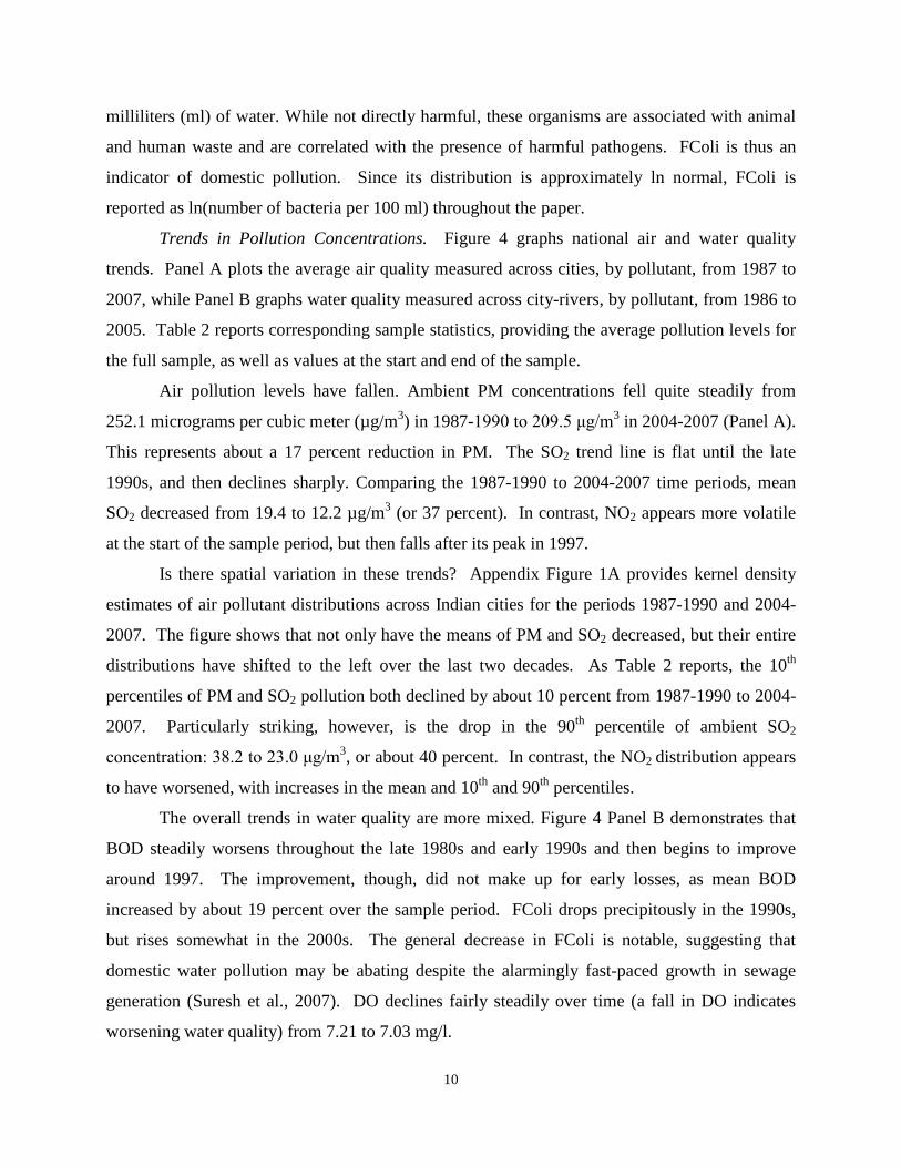
milliliters (ml) of water. While not directly harmful, these organisms are associated with animal
and human waste and are correlated with the presence of harmful pathogens. FColi is thus an
indicator of domestic pollution. Since its distribution is approximately ln normal, FColi is
reported as ln(number of bacteria per 100 ml) throughout the paper.
Trends in Pollution Concentrations. Figure 4 graphs national air and water quality
trends. Panel A plots the average air quality measured across cities, by pollutant, from 1987 to
2007, while Panel B graphs water quality measured across city-rivers, by pollutant, from 1986 to
2005. Table 2 reports corresponding sample statistics, providing the average pollution levels for
the full sample, as well as values at the start and end of the sample.
Air pollution levels have fallen. Ambient PM concentrations fell quite steadily from
252.1 micrograms per cubic meter (µg/m3) in 1987-1990 to 209.5 μg/m3 in 2004-2007 (Panel A).
This represents about a 17 percent reduction in PM. The SO2 trend line is flat until the late
1990s, and then declines sharply. Comparing the 1987-1990 to 2004-2007 time periods, mean
SO2 decreased from 19.4 to 12.2 µg/m3 (or 37 percent). In contrast, NO2 appears more volatile
at the start of the sample period, but then falls after its peak in 1997.
Is there spatial variation in these trends? Appendix Figure 1A provides kernel density
estimates of air pollutant distributions across Indian cities for the periods 1987-1990 and 2004-
2007. The figure shows that not only have the means of PM and SO2 decreased, but their entire
distributions have shifted to the left over the last two decades. As Table 2 reports, the 10th
percentiles of PM and SO2 pollution both declined by about 10 percent from 1987-1990 to 2004-
2007. Particularly striking, however, is the drop in the 90th percentile of ambient SO2
concentration: 38.2 to 23.0 μg/m3, or about 40 percent. In contrast, the NO2 distribution appears
to have worsened, with increases in the mean and 10th and 90th percentiles.
The overall trends in water quality are more mixed. Figure 4 Panel B demonstrates that
BOD steadily worsens throughout the late 1980s and early 1990s and then begins to improve
around 1997. The improvement, though, did not make up for early losses, as mean BOD
increased by about 19 percent over the sample period. FColi drops precipitously in the 1990s,
but rises somewhat in the 2000s. The general decrease in FColi is notable, suggesting that
domestic water pollution may be abating despite the alarmingly fast-paced growth in sewage
generation (Suresh et al., 2007). DO declines fairly steadily over time (a fall in DO indicates
worsening water quality) from 7.21 to 7.03 mg/l.

11
The distributions of the water pollutants across cities and their changes are presented in
Appendix Figure 1B, which comes from kernel density estimation. The distribution of BOD has
widened over the last twenty years, with many higher readings in the later time period.16
C. Infant Mortality Rate Data
While
the 10th percentile of BOD has dropped slightly, the 90th percentile has increased from 5.78 to
7.85 mg/l between the earlier and more recent periods. In contrast, the FColi distribution has
largely shifted to the left. The relatively clean cities show tremendous drops in FColi levels, with
the 10th percentile value falling from 3.61 to 1.79, while dirtier cities show more modest
declines. Lastly, the DO distribution does not appear to have changed noticeably, with very little
difference between the distributions from the earlier and later periods.
We obtained annual city-level infant mortality data from annual issues of Vital Statistics
of India for the years prior to 1996.17 In subsequent years, the city-level data were no longer
complied centrally; therefore, we visited the registrar’s office for each of India’s larger states and
collected the data directly.18 Many births and deaths are not registered in India and the available
evidence suggests that this problem is greater for deaths, so the infant mortality rate is likely
downward-biased. Although the infant mortality rate from the Vital Statistics data is about a
third of the rate measured from state-level survey measures of infant mortality rates (i.e., the
Sample Registration System), trends in the Vital Statistics and survey data are highly correlated.
While these data are likely to be noisy, there is no reason to expect that the measurement error is
correlated with the pollution measures.19
Infant mortality rates are an appealing measure of the effectiveness of environmental
regulations for at least two reasons. First, relative to measures of adult health, infant health is
likely to be more responsive to short and medium changes in pollution. Second, the first year of
life is an especially vulnerable one, and so losses of life expectancy may be large.
Since 1987, infant mortality has fallen sharply in urban India (Panel C of Figure 4). As
Panel C of Table 2 shows, the infant mortality rate fell from 29.6 per 1,000 live births in 1987-
16 The right tail of the 2002-2005 period extends to 100 mg/l, but the figure has been truncated at 20 mg/l to give a more detailed picture of the distribution. 17 We digitized the city-level data from the books. All data were double entered and checked for consistency. 18 Specifically, we attempted to obtain data in all states except the Northeastern states (which have travel restrictions) and Jammu-Kashmir. We were able to obtain data from Andhra Pradesh, Chandigarh, Delhi, Goa, Gujarat, Himachal Pradesh, Karnataka, Kerala, Madhya Pradesh, Maharashtra, Punjab, Rajasthan, and West Bengal. 19 Burgess et al. (2011) show that these mortality data are correlated with inter-annual temperature variation, providing further evidence that there is signal in these data.

12
1990 to 16.7 in 2001-2004. The kernel density graphs of infant mortality from the earlier and
later periods further confirm the reduction in mortality rates (Appendix Figure 1C).
D. Demographics Characteristics, Corruption, and Newspaper Pollution References
We additionally collected data on socio-demographic characteristics, corruption, and
social activism at the city-level. Socio-demographic data come from two sources.20
We used a variety of novel resources to develop measures of demand for clean air and
water and the degree of local corruption or institutional quality. First, we collected mentions on
“air pollution” and “water pollution” from the Times of India, the largest newspaper in India, by
state-year. Data prior to 2003 were obtained from the University of Pennsylvania’s searchable
library database, while data afterward were obtained from the Times of India’s online public
searchable database. We interpret the pollution mentions as indicators for the demand for clean
air and water but, as we discuss below, note that these measures may also be subject to other
reasonable interpretation. Systematic data on the degree of corruption across cities, as well as
measures of social activism, are notoriously difficult to obtain, particularly for developing
countries (Banerjee, Hanna and Mullainathan, forthcoming). We found and compiled data from
two sources. We conducted analogous newspaper searches from the Times of India, but in this
case searched for “corruption”, “graft”, and “embezzlement”, all of which are intended to
provide a proxy for institutional quality. Second, we collected data from Transparency
International on public perceptions of corruption by state for 2005.
First, we
obtained district-level data on population and literacy rates from the 1981, 1991, and 2001
Censuses of India. For non-census years, we linearly interpolated these variables. Second, we
collected district-level expenditure per capita data, which is a proxy for income. The data come
from the survey of household consumer expenditure carried out by India's National Sample
Survey Organization in the years 1987, 1993, and 1999 and are imputed in the missing years.
IV. Econometric Approach
This section describes a two-stage econometric approach for assessing whether India’s
regulatory policies impacted air and water pollution concentrations. The first-stage is an event
study-style equation:
20 Consistent city-level data in India is notoriously difficult to obtain. We instead acquired district level data, and matched cities to their respective districts.
13
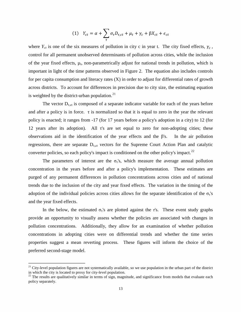
(1) 𝑌𝑐𝑡 = 𝛼 + �𝜎𝜏𝐷𝜏,𝑐𝑡 + 𝜇𝑡 + 𝛾𝑐 + β𝑋𝑐𝑡 + 𝜖𝑐𝑡𝜏
where Yct is one of the six measures of pollution in city c in year t. The city fixed effects, 𝛾𝑐 ,
control for all permanent unobserved determinants of pollution across cities, while the inclusion
of the year fixed effects, µt, non-parametrically adjust for national trends in pollution, which is
important in light of the time patterns observed in Figure 2. The equation also includes controls
for per capita consumption and literacy rates (X) in order to adjust for differential rates of growth
across districts. To account for differences in precision due to city size, the estimating equation
is weighted by the district-urban population.21
The vector Dτ,ct is composed of a separate indicator variable for each of the years before
and after a policy is in force. τ is normalized so that it is equal to zero in the year the relevant
policy is enacted; it ranges from -17 (for 17 years before a policy's adoption in a city) to 12 (for
12 years after its adoption). All τ's are set equal to zero for non-adopting cities; these
observations aid in the identification of the year effects and the β's. In the air pollution
regressions, there are separate Dτ,ct vectors for the Supreme Court Action Plan and catalytic
converter policies, so each policy's impact is conditioned on the other policy's impact.
22
The parameters of interest are the στ's, which measure the average annual pollution
concentration in the years before and after a policy's implementation. These estimates are
purged of any permanent differences in pollution concentrations across cities and of national
trends due to the inclusion of the city and year fixed effects. The variation in the timing of the
adoption of the individual policies across cities allows for the separate identification of the στ's
and the year fixed effects.
In the below, the estimated στ's are plotted against the τ's. These event study graphs
provide an opportunity to visually assess whether the policies are associated with changes in
pollution concentrations. Additionally, they allow for an examination of whether pollution
concentrations in adopting cities were on differential trends and whether the time series
properties suggest a mean reverting process. These figures will inform the choice of the
preferred second-stage model.
21 City-level population figures are not systematically available, so we use population in the urban part of the district in which the city is located to proxy for city-level population. 22 The results are qualitatively similar in terms of sign, magnitude, and significance from models that evaluate each policy separately.
14
The sample for equation (1) is based on the availability of data for a particular pollutant
in a city. For adopting cities, a city is included in the sample if it has at least one observation
three or more years before the policy's enactment and four or more years afterward. If a city
does not have any post-adoption observations or did not enact the relevant policy, then that city
is required to have at least two observations for inclusion in the sample.
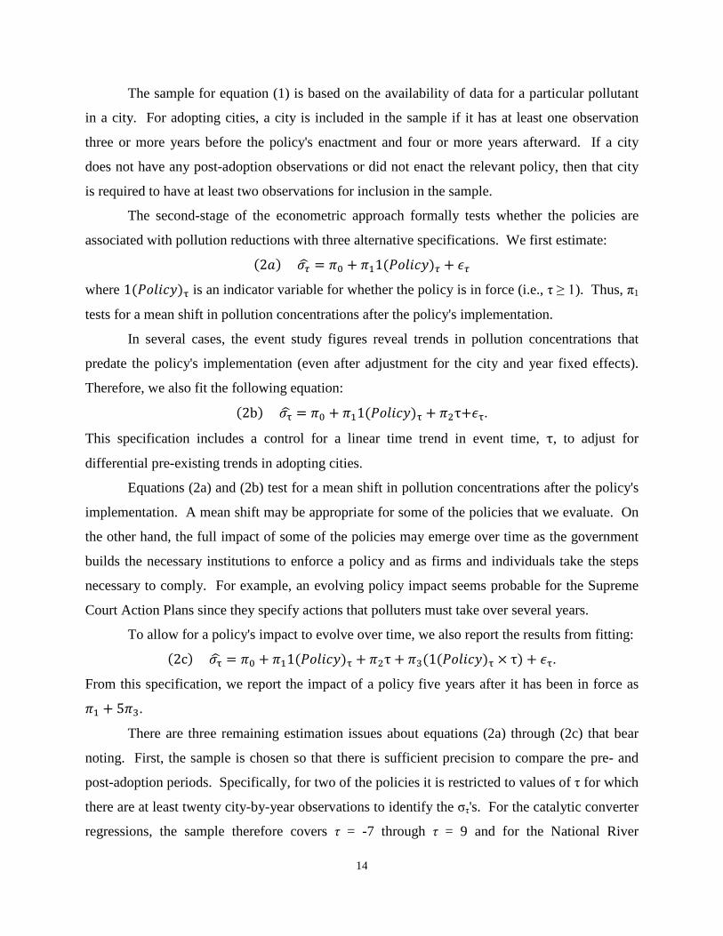
The second-stage of the econometric approach formally tests whether the policies are
associated with pollution reductions with three alternative specifications. We first estimate:
(2𝑎) 𝜎𝜏� = 𝜋0 + 𝜋11(𝑃𝑜𝑙𝑖𝑐𝑦)𝜏 + 𝜖𝜏 where 1(𝑃𝑜𝑙𝑖𝑐𝑦)τ is an indicator variable for whether the policy is in force (i.e., τ ≥ 1). Thus, π1
tests for a mean shift in pollution concentrations after the policy's implementation.
In several cases, the event study figures reveal trends in pollution concentrations that
predate the policy's implementation (even after adjustment for the city and year fixed effects).
Therefore, we also fit the following equation:
(2b) 𝜎τ� = 𝜋0 + 𝜋11(𝑃𝑜𝑙𝑖𝑐𝑦)τ + 𝜋2τ+𝜖τ.
This specification includes a control for a linear time trend in event time, τ, to adjust for
differential pre-existing trends in adopting cities.
Equations (2a) and (2b) test for a mean shift in pollution concentrations after the policy's
implementation. A mean shift may be appropriate for some of the policies that we evaluate. On
the other hand, the full impact of some of the policies may emerge over time as the government
builds the necessary institutions to enforce a policy and as firms and individuals take the steps
necessary to comply. For example, an evolving policy impact seems probable for the Supreme
Court Action Plans since they specify actions that polluters must take over several years.
To allow for a policy's impact to evolve over time, we also report the results from fitting:
(2c) 𝜎τ� = 𝜋0 + 𝜋11(𝑃𝑜𝑙𝑖𝑐𝑦)τ + 𝜋2τ + 𝜋3(1(𝑃𝑜𝑙𝑖𝑐𝑦)τ × τ) + 𝜖τ.
From this specification, we report the impact of a policy five years after it has been in force as
𝜋1 + 5𝜋3.
There are three remaining estimation issues about equations (2a) through (2c) that bear
noting. First, the sample is chosen so that there is sufficient precision to compare the pre- and
post-adoption periods. Specifically, for two of the policies it is restricted to values of τ for which
there are at least twenty city-by-year observations to identify the στ's. For the catalytic converter
regressions, the sample therefore covers τ = -7 through τ = 9 and for the National River
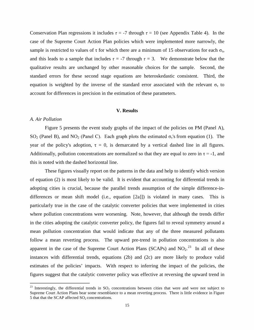
15
Conservation Plan regressions it includes τ = -7 through τ = 10 (see Appendix Table 4). In the
case of the Supreme Court Action Plan policies which were implemented more narrowly, the
sample is restricted to values of τ for which there are a minimum of 15 observations for each στ,
and this leads to a sample that includes τ = -7 through τ = 3. We demonstrate below that the
qualitative results are unchanged by other reasonable choices for the sample. Second, the
standard errors for these second stage equations are heteroskedastic consistent. Third, the
equation is weighted by the inverse of the standard error associated with the relevant στ to
account for differences in precision in the estimation of these parameters.
V. Results
A. Air Pollution
Figure 5 presents the event study graphs of the impact of the policies on PM (Panel A),
SO2 (Panel B), and NO2 (Panel C). Each graph plots the estimated στ's from equation (1). The
year of the policy's adoption, τ = 0, is demarcated by a vertical dashed line in all figures.
Additionally, pollution concentrations are normalized so that they are equal to zero in τ = -1, and
this is noted with the dashed horizontal line.
These figures visually report on the patterns in the data and help to identify which version
of equation (2) is most likely to be valid. It is evident that accounting for differential trends in
adopting cities is crucial, because the parallel trends assumption of the simple difference-in-
differences or mean shift model (i.e., equation [2a]]) is violated in many cases. This is
particularly true in the case of the catalytic converter policies that were implemented in cities
where pollution concentrations were worsening. Note, however, that although the trends differ
in the cities adopting the catalytic converter policy, the figures fail to reveal symmetry around a
mean pollution concentration that would indicate that any of the three measured pollutants
follow a mean reverting process. The upward pre-trend in pollution concentrations is also
apparent in the case of the Supreme Court Action Plans (SCAPs) and NO2.23
23 Interestingly, the differential trends in SO2 concentrations between cities that were and were not subject to Supreme Court Action Plans bear some resemblance to a mean reverting process. There is little evidence in Figure 5 that that the SCAP affected SO2 concentrations.
In all of these
instances with differential trends, equations (2b) and (2c) are more likely to produce valid
estimates of the policies’ impacts. With respect to inferring the impact of the policies, the
figures suggest that the catalytic converter policy was effective at reversing the upward trend in

16
pollution concentrations, while the SCAPs appear ineffective, with the possible exception of
NO2.
Table 3 provides more formal tests by reporting the key coefficient estimates from fitting
equations (2a) - (2c). For each pollutant-policy pair, the first column reports the estimate of π1
from equation (2a), which tests whether στ is on average lower after the implementation of the
policy. The second column reports the estimate of π1 and π2 from the fitting of equation (2b) in
the second column for each pollutant. Here, π1 tests for a policy impact after adjustment for the
trend in pollution levels (π2). The third column reports the results from equation (2c) that allow
for a mean shift and trend break after the policy’s implementation. It also reports the estimated
effect of the policy five years after their implementation, which is equal to 𝜋1 + 5𝜋3.
Reading across Panel A, it is evident that the SCAPs have a mixed record of success.24
In contrast, the regressions confirm the visual impression that the catalytic converter
policies were strongly associated with air pollution reductions. In light of the differential pre-
trends in pollution in adopting cities and that the policy's impact will only emerge as the stock of
cars changes, the richest specification (equation [2c]) is likely to be the most reliable. It
indicates that 5 years after the policy was in force, PM, SO2, and NO2 declined by 48.6 µg/m3,
13.4 µg/m3, and 4.5 µg/m3, respectively. The PM and SO2 declines are statistically significant
when judged by conventional criteria, while the NO2 decline is not. These declines are 19
percent, 69 percent, and 15 percent of the 1987-1990 nationwide mean concentrations,
respectively. These percentage declines are large, reflecting the rapid rates at which ambient
pollution concentrations were increasing before the policy’s implementation in adopting cities—
put another way, if the pre-trends had continued then pollution concentrations would have
reached levels much higher than those recorded in the 1987-1990 period.
There is little evidence of an impact on PM or SO2 concentrations. The available evidence for an
impact comes from the NO2 regressions that control for pre-existing trends. In column (8) the
estimated impact would not be judged statistically significant, while in column (9) it is of a large
magnitude and would be judged marginally significant.
Appendix Table 4 demonstrates that the qualitative results are unchanged by reasonable
alternative sample selection rules that determine the number of event years included in the 24 Note that for the Supreme Court Action Plans, the analysis lags the policies by one year. The dates we have correspond to Court Orders, which mandated submission of Action Plans. However, a special committee frequently reviewed the SCAPs and only afterwards declared/implemented them.
17
analysis.25
B. Effects of Policies on Water Quality
Specifically, we fit equation (2c) on a wider range of τ's (i.e., from τ = -9 through τ =
9 for the catalytic converters and τ = -14 through τ = 4 for the SCAPs) and a narrower range τ's
(i.e., from τ = -5 through τ = 5 for the catalytic converters and τ = -4 through τ = 4 for the
SCAPs). The pattern of the coefficients for the catalytic converters policy is similar to that of
Table 3 for both the wider and narrower event year samples. The SCAP is associated with a
large and significant decline in NO2 with the narrower range. With the wider range, the SCAP
continues to be associated with a decline in NO2 but it no longer would be judged to be
statistically significant; however, it is associated with a statistically significant decline in PM.
Panels A-C of Figure 6 present event study analyses of the impact of the National River
Conservation Plan (NRCP) on BOD, ln(FColi), and DO, respectively. As in Figure 5, the figures
plot the results from the estimation of equation (1). From the figures, there is little evidence that
the NRCP was effective at reducing pollution concentrations.
Table 4 provides the corresponding regression analysis and is structured similarly to
Table 3. The evidence in favor of a policy impact is weak. BOD concentrations are lower after
the implementation of NRCP, but the decline occurs several years prior to the implementation of
the plan (Panel A). While NRCP targets domestic pollution, the data fail to reveal an
improvement in FColi concentrations (Panel B), which is the best measure of domestic sourced
water pollution. The results from the fitting of equation (2c) are reported in column (9) and
confirm the perverse visual impression that the NRCP is associated with a worsening in DO
concentrations (recall, lower DO levels indicate higher pollution concentrations).26
C. Assessing Robustness with a Structural Break Test
The previous subsection presented results from a difference-in-differences (DD)
approach that can accommodate differential trends across cities that did and did not adopt the
25 There is a tradeoff to including a greater or smaller number of event years or τ's in the second-stage analysis. The inclusion of a wider range of τ's provides a larger sample size and allows for more precise estimation of pre and post adoption trends. But at the same time, it moves further away from the event in question so that other unobserved factors may confound the estimation of the policy effects. Further, it exacerbates the problems associated with estimating the τ's from an unbalanced panel data file of cities. In contrast, the inclusion of fewer τ's results in a smaller sample size (and number of cities) to estimate pre and post trends, but the analysis is more narrowly focused around the policy event. Appendix Table 3 reports on the number of city-by-year observations that identify the στ's associated with each event year. 26 Appendix Table 4 demonstrates that the qualitative result that the NRCP had little impact on the available measures of water pollution is unchanged by reasonable alternative selection rules for the number of event years to include in the analysis. The table reports on specifications that increase and decrease the number of event years or taus (i.e., changing the event years to include [-9,12] or to include [-5,5]) in the second-stage analysis.

18
environmental regulations. As is always the case with a non-experimental design, there is a form
of unobserved heterogeneity that can explain the findings without a causal explanation. This
subsection adapts a structural break test from time-series econometrics and demonstrates that
these tests can be used to shed light on the validity of a DD-style design. Structural break tests
have generally been limited to settings where this is a single time-series and a control group is
unavailable. However as equation (1) and the event-study figures highlight, it is straightforward
to collapse a DD framework into a single time-series, even when the policy date varies across
units (i.e., cities in our setting) that have been adjusted for unit and time fixed effects. We are
unaware of previous efforts to apply structural break tools to a DD setting and believe that these
tests can and should be used more broadly with DD designs.27
Inspired by Piehl et al. (2003), we adapt the Quandt likelihood ratio (QLR) statistic to
determine if there is a structural break in a time-series. Specifically, we take the estimated στ's
from the estimation of equation (1) and the most robust second-stage specification (i.e., [2c]) that
assumes that the regulations cause a mean shift and trend break in pollution concentrations. Note
that the test for whether a policy has any effect in equation (2c) is tantamount to calculating the
F-statistic associated with the null hypothesis that 𝜋1 = 0 and 𝜋3 = 0. In time-series, this is
often referred to as a Chow-test for parameter constancy, but it essentially boils down to an F-
test.
The idea is to assess whether there is a structural break in the policy parameters (i.e.,
𝜋1 and 𝜋3) near the true date of the policy’s adoption. The test does two things: It identifies the
date at which there is the largest change in the parameters (defined as the date associated with
the largest change in the F-statistic) and produces p-values for whether the change in those
parameters is different than zero (i.e., whether there is a break). A failure to find a break or a
finding of a break significantly before the measured date of policy implementation would
suggest that the policies were ineffective and undermine any findings to the contrary from the
DD approach. In contrast, a finding of a policy effect in the years around τ = 0, especially the
years after τ = 0, would support the findings of a policy effect from the DD results.
This test is implemented in two steps. First, equation (2c) is re-estimated redefining a
new “policy implementation” date each time and the F-statistic associated with the null 27 Based on our investigation, the closest use of a structural break test in a non-time series setting is Ludwig and Miller’s (2007) application within a regression discontinuity framework as a robustness check for the existence and timing of a discontinuity.

19
hypothesis that 𝜋1 = 0 and 𝜋3 = 0 is calculated. We test for break dates within a window of the
middle 50 percent of the event years in each time-series. There needs to be a sufficient amount
of data outside the window, so, for example, the possible break dates are limited to τ = -3
through τ = 6 (out of the total available years that range from τ = -7 through τ = 9) for the effect
of the catalytic converter policy on PM.
Second, the QLR test selects the maximum of the F-statistics to test for a break at an
unknown date. The maximum of a number of F-statistics does not converge to any known
distribution. Andrews (1993) provides critical values that are asymptotically correct, but we
instead run a Monte Carlo simulation to compute the critical values due to our small sample.
Specifically, to compute the small-sample critical values, we first generated data with the
variance set equal to the variance of the actual data, but without a break in the data. We then
compute the QLR test over the simulated data to obtain the maximum F-statistics. We replicate
this 100,000 times to obtain the distribution of the QLR statistics under a null of hypothesis of no
break.
Figure 7 and Table 5 (Panel A) report on the results of the QLR test for the catalytic
converter policy, which the previous section found to be the most effective policy. For PM,
Panel A of Figure 7 plots the F-statistics associated with the test of a break for each of the event
years. It is evident that this test selects τ = 2 as the event year with the most substantive break.
Table 5 reports that the null hypothesis of no break at τ = 2 can be rejected at the 1 percent level.
This break corresponds to the reversal of the upward trend in PM observed at τ = 2 in Figure 5.
The results from the other two structural break tests are also broadly supportive of the
previous subsection’s findings. With respect to SO2, Panel B of Figure 7 reveals that the largest
F-statistics are concentrated in the period τ = -2 through τ = 1. The QLR statistic (i.e., the biggest
F-statistic) occurs at τ = -1 and is easily statistically significant at the 1 percent level (Table 5).
A comparison of this figure and Figure 5 reveal that the QLR test, which is only designed to test
for a single break, picks the arrest of the upward trend in SO2 as a more important change than
the downward trend that is first evident in τ = 1. Overall, the test suggests that the case for the
catalytic converter policy reducing SO2 concentrations is not as strong as the case for a
relationship between the policy and reduced PM concentrations. Finally, Panel C of Figure 7
and Table 5 fail to provide evidence of a structural break in NO2 concentrations, which is
consistent with Table 3 where the null of zero effect cannot be rejected.

20
For comparison, Panel B of Table 5 provides the QLR test statistics for the National
River Conservation Policy. The null of no structural break cannot be rejected for the BOD or
Ln(Fcoli) time series, which is consistent with the results in Table 4. There is a significant break
in DO, but it occurs three years prior to the event; this is consistent with the observed worsening
of DO that, according to the event study analysis in Figure 6, begins about three years prior to
the program implementation. Finally, we note that we could not conduct the QLR test for the
SCAPs due to the limited number of event years for these policies.
D. Effects of Catalytic Converter Policy on Infant Mortality
The catalytic converter policy is the most strongly related to improvements in air
pollution. This subsection explores whether the catalytic converter policy is associated with
changes in human health, as measured by infant mortality rates.
Specifically, we fit equation (1) and equations (2a) - (2c), where the infant mortality rate
is the outcome of interest. Several estimation details are noteworthy. First, despite a large data
collection exercise (including going to each state to obtain additional registry data), there are
fewer cities in the sample.28
Figure 8 and Table 6 report the results. In light of the differential pre-existing trend, the
column (3) specification is likely to be the most reliable. It suggests that the catalytic converter
policy is associated with a reduction in the infant mortality rate of 0.86 per 1,000 live births.
However, this estimate is imprecise and is not statistically significant.
Second, the dependent variable is constructed as the ratio of infant
deaths to births, and equation (1) is weighted by the number of births in the city-year. Third, it is
natural to consider using the catalytic converter induced variation to estimate the separate
impacts of each of the three forms of air pollution on infant mortality in a two-stage least squares
setting. However, such an approach is invalid in this setting because, even when the exclusion
restriction is otherwise valid, there is a single instrument for three endogenous variables.
VI. Why Were the Air Pollution Policies More Effective than the Water Pollution Policies?
The previous section’s results’ analysis indicates that India’s air pollution policies were
more successful than the water pollution ones. The question that naturally arises is why? India
has an extensive history of both types of policies, and, in fact, the National Water Act—giving
28When the air pollution sample is restricted to the sample used to estimate the infant mortality equations, the catalytic converter policy is associated with substantial reductions in PM and SO2 but not of NO2 concentrations.

21
the government the rights and official structure in which to regulate water pollution—was passed
seven years before the Air Act. This section presents qualitative and quantitative evidence that
suggests that the difference is largely a reflection of the greater demand for clean air.
A. Qualitative Evidence
There are several reasons why the demand for better air quality may exceed that for
water. First, the costs of air pollution may be higher: The Global Burden of Disease study (Lim
et al., 2012) suggests that outdoor PM and ozone air pollution are responsible for about 3.4
million premature fatalities annually. In contrast, the estimated number of annual premature
fatalities due to unimproved water and sanitation (i.e., about 340,000) is an order of magnitude
smaller. Further, recent evidence indicates that the mortality impacts of poor air quality at the
high concentrations observed in many Indian cities may be worse than previously recognized
(Chen et al., 2013).
The second, and related, reason may be a difference in avoidance costs. The argument
starts with the observation that middle and upper income groups are the most likely to engage in
public activism on environmental issues, and these groups may find it relatively easy to avoid
water pollution through the purchase of clean, bottled water. In fact, the revenue generated from
bottled water sales in India in 2010 exceeded $250 million dollars and was “expected to grow at
a 30% rate in the next 7 years.”29
Third, air pollution appears to have been a greater source of concern in public discourse,
suggesting relatively greater demand for air quality. We collected data from the Times of India,
which is the most widely read English-language newspaper in India (and the world), on the
number of mentions of air and water pollution. Figure 9 demonstrates that air pollution was
mentioned about three times as frequently as water pollution between 1986 and 2007.
Further, it is common for middle-class households to use
boiling and other techniques for cleaning water. In contrast, it is nearly impossible to completely
protect oneself against air pollution because people spend time outdoors for leisure, travel to
work, etc., and air pollution can penetrate buildings and affect indoor air quality.
30
Fourth, the implementation and enforcement of the water pollution regulations, compared
While
this finding is consistent with higher demand for air quality, it is possible that the greater
mentions reflect differences in water or air pollution concentrations or some other factor.
29 http://www.researchandmarkets.com/research/f9deab/indian_bottled_wat, accessed on August 14, 2012. 30 Interestingly, this finding still holds even when reports from Delhi, which had especially poor air quality, are dropped.
22
to the air pollution regulations, suggest a relatively lower demand for water quality. For starters,
the lines of authority under the NRCP for the designation of water quality standards and their
enforcement were muddled and unclear. No single organization was accountable for ensuring
success: Although the NRCP was originally developed and launched by the MoEF,
implementation and enforcement were split among a wide variety of institutions that frequently
lack the power necessary for successful enforcement, including the CPCB, the State Pollution
Control Boards, and local departments for public health, development, water, and sewage
(Ministry of Environment and Forests, 2006). Additionally, the recommended solutions to high
water pollution concentrations involve the construction of sewage treatment plants and other
expensive capital investments, but the legislation did not provide a dedicated source of revenues
and funding responsibility jumped around across levels of government during this period.31
Further, state and local bodies have been accused of financial mismanagement, including
diversion, underutilization, and incorrect reporting of funds (Ministry of Environment and
Forests, 2006). The weak institutional support for the NRCP was evident in the failure to
achieve basic “process” goals, such as construction of necessary sewage treatment plants.32
In principle, air pollution laws had many of the same jurisdictional and enforcement
issues, but the key difference is that they often had the forceful support of India’s Supreme
Court. This difference is a critical one because the Supreme Court has the role of determining
when there have been serious infringements of fundamental and human rights. The avenue for
such determinations is India’s public interest litigation that can compel the Supreme Court to
deliver economic and social rights that are protected by the constitution but are otherwise
unenforceable. Notably, a public interest litigation suit can be introduced by an aggrieved party,
a third party (e.g., a non-governmental organization), or even the Supreme Court itself. In many
instances, the Supreme Court’s rulings have been motivated by executive inaction.
India’s Supreme Court became heavily involved in environmental affairs with its order
31 Under the first river Action Plan in 1985, the central government was responsible for 100 percent of policy funding. In 1990, it was decided that the cost would be split between central and state administrations. This division was revoked in 1997, returning the full cost to the Union government. One final change was made in 2001, allocating 30 percent of the financial burden to states, a third of which was levied on local bodies themselves (Suresh et al., 2007, p. 3). 32 For example as of March 2009, 152 out of 165 towns officially covered under NRCP have been approved for Sewage Treatment Plant capacity building, but construction has been initiated in only 82. Additionally, as of March 2009, there has not been any spending of federal or state monies on the NRCP in fifteen NRCP towns (National River Conservation Directorate, 2009). Furthermore, the Centre for Science and Environment (CSE) calculates that the 2006 treatment capacity was only 18.5 percent of the full sewage burden (Suresh et al., 2007, p. 11)

23
that Delhi develop an action plan to address pollution in 1996.33
In summary, the air pollution regulations had the powerful Supreme Court’s backing and
this brought substantial bureaucratic effort to bear on the problem.
The Court followed that order
with a directive to create an authority “to advise the court on pollution and monitor
implementation of its order.” Following the success of the Delhi efforts, new initiatives to
address pollution were pushed forward by non-governmental organizations, public sentiment,
prominent Indian citizens, and the Supreme Court. These efforts ultimately led to further action
by the Supreme Court, including requirements for city-level Supreme Court Action Plans, the
mandatory installation of catalytic converters for designated cities, and other regulatory and
enforcement efforts.
34 In contrast, the
implementation and enforcement of the water pollution regulation appeared to lack widespread
public support and was left to a mix of central and state government institutions without the
tools, accountability, and resources that are generally critical for effective governance. Our read
of the history is that the Supreme Court’s decision to focus on air pollution, and largely ignore
water pollution, reflects the higher level of demand for government provision of improved air
quality that manifested itself as public activism and citizen suits filed in the Supreme Court
under the aegis of India’s public interest litigation.35
B. Quantitative Evidence
This subsection quantitatively assesses the hypothesis developed in the previous
subsection that the greater success of air pollution policies was due to higher demand for
improvement in air quality. This exercise is conducted by dividing the sample of cities into
those with above and below the median value of variables that can be interpreted as demand
shifters for air quality. Given that corruption is often cited as a barrier to the efficient delivery of
government services in developing countries, we also test whether the air pollution policies were
more effective in cities with above, versus below, median values of variables designed to
measure the degree of local corruption (see, for example, Banerjee, Hanna, and Mullainathan,
forthcoming). 33 It has been suggested that the mandate for an action plan to address pollution in Delhi was partially due to Justice Kuldeep Singh reading a book published by the influential NGO Centre for Science and Environment, entitled Slow Murder: The Deadly Story of Vehicular Pollution in India (Narain and Bell, 2005, p. 10). 34 A former CPCB chairman summed up the need for Supreme Court intervention: “When it comes to doing things, it is not up to the CPCB, even in the area of air pollution.” (Sharma and Roychowdhury, 1996, p. 128). 35 As just one prominent example, see Court Order on April 5th, 2002, Supreme Court of India. Writ Petition (Civil) No. 13029 of 1985. M.C. Mehta vs. Union of India and Others.

24
Table 7 reports the results from the estimation of equation (2c) for the success of the
catalytic converter policy.36
The results are consistent with the hypothesis that differences in the demand for air
quality drive the effectiveness of the air pollution policies. Turning first to literacy, columns (1)
and (2) reveal that the catalytic converter policy is associated with larger 5-year reductions in
PM and SO2 concentrations in cities with higher literacy rates, although 95% confidence
intervals overlap in both cases. Similarly, we find larger policy impacts in cities with more
frequent mentions of air pollution in the Times of India (Columns [3] and [4]). In contrast,
columns (5) – (8) fail to reveal a consistent pattern, suggesting that the available measures of
corruption are unrelated to the effectiveness of the catalytic converter policy.
In columns (1) and (2), the samples are restricted to cities with
education levels that are above and below the median, respectively; we assume that education is
a proxy for higher demand for air quality due to higher knowledge on the health effects of air
quality and/or higher income. Columns (3) and (4) repeat this exercise, but this time we divide
cities by the number of mentions of air pollution (measured at the state-level) in the Times of
India. We interpret the newspaper mentions as a measure of demand for clean air, although it
would be inappropriate to definitively rule out that the mentions reflect other factors that cannot
be classified as demand shifters (e.g., newspaper mentions may provide new information that in
turn increase demand for air quality). Columns (5) - (8) repeat this exercise for two different
measures of corruption: The sample is divided in half by the number of mentions of corruption in
the Times of India and Transparency International’s corruption rankings, respectively.
37
VII. Conclusion
Using the most comprehensive data file ever compiled on air pollution, water pollution,
environmental regulations, and infant mortality for a developing country, this paper tests for the
impacts of key air and water pollution regulations in India. We find that air regulations were in
part responsible for observed improvements in air quality over the last two decades. The most
successful air regulation resulted in a modest, but statistically insignificant decline in infant
mortality. In contrast to the air findings, the results indicate that the National River Conservation
36 As in the main analysis, all regressions are estimated by OLS and include indicators for the Supreme Court Action Plans in the first stage, and have robust standard errors in the second stage. 37 Table 7’s results are unchanged qualitatively if cities are divided by the per-capita Times of India mentions of air pollution and corruption, rather than the raw number of mentions.
25
Plan—the cornerstone of India’s water policies—failed to lead to improvements in any of the
three available measures of water pollution.
India, like many developing countries, is widely considered to have weak regulatory
institutions, so the success of the air policies is noteworthy. A range of qualitative and
quantitative evidence suggests that citizens’ higher relative demand for air quality, especially
those with the means to file public interest litigation suits, were critical to the air regulations'
success. This demand and activism prompted the Supreme Court, which is widely considered
the country's most efficacious institution, to become active in the implementation and
enforcement of the air regulations.
There are several broader implications. First, the results demonstrate that environmental
regulations and presumably other government interventions can succeed, even in weak
institutional settings, when demand and/or public support is strong enough. Second, the results
suggest that no matter what climate deals are worked out internationally, India may be unlikely
to significantly reduce greenhouse gas emissions until climate change becomes an urgent issue
domestically. This would pose challenges for addressing climate change because India is
projected to be a major contributor to the growth in greenhouse gas emissions in the coming
decades. Third, the paper has left unanswered the fundamental questions of the magnitudes of
the marginal benefits and costs of regulation-induced emissions reductions and whether the
benefits exceed the costs. Currently, there is very limited information on the costs and benefits
of environmental regulations in developing countries and this is a rich area for future research.
REFERENCES
Alpert, Pinhas, Olga Shvainshtein, and Pavel Kishcha. 2012. “AOD Trends over Megacities Based on Space Monitoring Using MODIS and MISR.” American Journal of Climate Change,1(3): 117-131.
Andrews, Donald W. K. 1993. “Tests for Parameter Instability and Structural Change with Unknown Change Point.” Econometrica, 61(4), 821-856.
Asian Development Bank. “Yamuna Action Plan – India,” in Asian Water Development Outlook 2007. Manila, Philippines: Asian Development Bank, 2007.
Banerjee, Abhijit, Rachel Glennerster, and Esther Duflo. 2008. “Putting a Band-Aid on a Corpse: Incentives for Nurses in the Indian Public Health Care System,” Journal of the European Economics Association, 6(2-3): 487–500.
Banerjee, Abhijit, Rema Hanna and Sendhil Mullainathan. forthcoming. “Corruption.” Handbook of Organizational Economics.
Bento, Antonio, Maureen, Cropper and Akie Takeuchi. 2007. “The Impact of Policies to Control Motor Vehicle Emissions in Mumbai, India.” Journal of Regional Science,

26
47(1): 27–46. Bertrand, Marianne, Simeon Djankov, Rema Hanna, and Sendhil Mullainathan. 2007.
“Obtaining a Driver's License in India: An Experimental Approach to Studying Corruption.” Quarterly Journal of Economics, 122 (4): 1639-1676.
Burgess, Robin, Olivier Deschenes, Dave Donaldson, and Michael Greenstone. 2011. “Weather and Death in India: Mechanisms and Implications for Climate Change.” Mimeo.
Cha, J. Mijin. 2005. “A Critical Examination of the Environmental Jurisprudence of the Courts of India,” Albany Law Environmental Outlook Journal, 10: 197.
Chay, Kenneth and Michael Greenstone. 2003. “Air Quality, Infant Mortality, and the Clean Air Act of 1970,” Mimeo.
Chay, Kenneth and Michael Greenstone. 2005. “Does Air Quality Matter? Evidence from the Housing Market,” Journal of Political Economy, 113(2).
Chen, Yuyu, Avraham Ebenstein, Michael Greenstone, and Hongbin Li. 2013. “The Long-Run Impact of Air Pollution on Life Expectancy: Evidence from China’s Huai River Policy,” Mimeo.
Cropper, Maureen. 2010. “What are the Health Effects of Air Pollution in China?” Is Economic Growth Sustainable? Palgrave Macmillan, New York, New York.
Cropper, Maureen, Shama Gamkhar, Kabir Malik, Alex Limonov, and Ian Partridge. 2012. The Health Effects of Coal Electricity Generation in India, Resources for the Future Discussion Paper No. 12-25.
Davis, Lucas W. 2008. "The Effect of Driving Restrictions on Air Quality in Mexico City." Journal of Political Economy, 116(1): 38-81.
Duflo, Esther, Michael Greenstone, Rohini Pande, and Nicholas Ryan. 2012. "Truth-telling by Third-Party Auditors and the Response of Polluting Firms: Experimental Evidence from India.” Mimeograph.
Environmental Performance Index. 2013. “2012 EPI and Pilot Trend Results: Air Pollution (effects on human health).” http://epi.yale.edu/dataexplorer/indicatorprofiles?ind=eh.air Accessed 2/4/13.
Foster, Andrew D., and Naresh Kumar. 2008. “Have CNG regulations in Delhi done their job?” Economic and Political Weekly, 42(51): 48-58.
Foster, Andrew D., and Naresh Kumar. 2009. “Air Quality Interventions and Spatial Dynamics of Air Pollution in Delhi and its Surroundings.” International Journal of Environment and Waste, 4(1/2): 85-111.
Greenstone, Michael. 2003. “Estimating Regulation-Induced Substitution: The Effect of the Clean Air Act on Water and Ground Pollution.” American Economic Review Papers and Proceedings, 93(2): 442-448.
Greenstone, Michael. 2004. “Did the Clean Air Act Amendments Cause the Remarkable Decline in Sulfur Dioxide Concentrations?” Journal of Environmental Economics and Management, 47.
Hadden, Susan G. 1987. “Statutes and Standards for Pollution Control in India,” Economic and Political Weekly, 22 (16): 709-711+713-720.
Hanna, Rema, and Paulina Oliva. 2010. "The Impact of Inspections on Plant-Level Air Emissions." The B.E. Journal of Economic Analysis and Policy, 10(1).
Hanna, Rema, and Paulina Oliva. 2011. “The Effect of Pollution on Labor Supply: Evidence from a Natural Experiment in Mexico City,” Mimeo.
Henderson, J. Vernon. 1996. "Effects of Air Quality Regulation." American Economic Review,
27
86: 789-813. Lim, Stephen S., et al. 2012. “A Comparative Rise Assessment of Burden of Disease and Injury
Attributable to 67 Risk Factors and Risk Factors in 21 Regions, 1990-2010.” The Lancet, 380: 2224-2260.
Ludwig, Jens, and Douglas Miller. 2007. “Does Head Start improve children’s outcomes? Evidence from a regression discontinuity design,” Quarterly Journal of Economics, 122(1): 159-208.
Meagher, J. Patrick. 1990. “Environmental Protection and Industries in Developing Countries: The Case of India Since Bhopal.” The Georgetown International Environmental Law Review, 3(1): 1-53.
Ministry of Environment and Forests. 2006. “26th Report of the Public Accounts Committee (Fourteenth Lok Sabha): Ganga Action Plan.” Presented to Lok Sabha on March 17th, 2006. Lok Sabha Secretariat: New Delhi.
Narain, Urvashi and Ruth Greenspan Bell. 2005. “Who Changed Delhi’s Air? The Roles of the Court and the Executive in Environmental Policymaking.” Resources for the Future Discussion Paper.
National River Conservation Directorate. “M.I.S. Report of Programmes Under National River Conservation Plan, Vol. III.” National River Conservation Directorate, Ministry of Environment and Forests, Government of India: New Delhi, March, 2009.
Oliva, Paulina. 2011. “Environmental Regulations and Corruption: Automobile Emissions in Mexico City," Mimeo.
Quandt, Richard E. 1960. “Tests of the Hypothesis That a Linear Regression System Obeys Two Separate Regimes.” Journal of the American Statistical Association, 55: 324-330.
Piehl, Anne Morrison, Suzanne Cooper, Anthony Braga and David Kennedy. 2003. “Testing for Structural Breaks in the Evaluation of Programs.” The Review of Economics and Statistics, 85(3): 550-558.
Sharma, Anju and Anumita Roychowdhury. Slow Murder: The deadly story of vehicular pollution in India. New Delhi : Centre for Science and Environment, 1996.
Smith, Steven J, Hugh Pitcher and T.M.L Wigley. 2001. “Global and regional anthropogenic sulfur dioxide emissions” Global and Planetary Change, 29 (1-2): 99–119.
Suresh, Babu S. V., Bharat L. Seth, Ajit Chak, Vasudha K. Dixit, and Sunita Narain. Sewage Canal: How to Clean the Yamuna. New Delhi: Centre for Science & Environment, 2007.
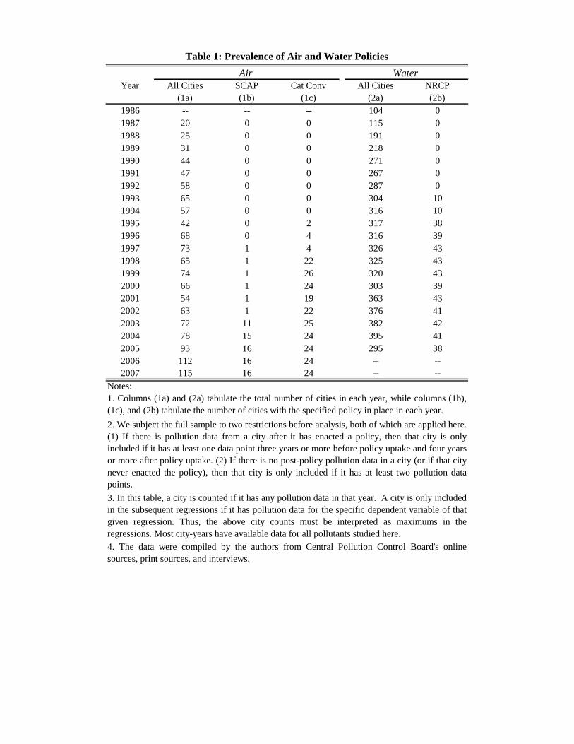
Year All Cities SCAP Cat Conv All Cities NRCP
(1a) (1b) (1c) (2a) (2b)
1986 -- -- -- 104 0
1987 20 0 0 115 0
1988 25 0 0 191 0
1989 31 0 0 218 0
1990 44 0 0 271 0
1991 47 0 0 267 0
1992 58 0 0 287 0
1993 65 0 0 304 10
1994 57 0 0 316 10
1995 42 0 2 317 38
1996 68 0 4 316 39
1997 73 1 4 326 43
1998 65 1 22 325 43
1999 74 1 26 320 43
2000 66 1 24 303 39
2001 54 1 19 363 43
2002 63 1 22 376 41
2003 72 11 25 382 42
2004 78 15 24 395 41
2005 93 16 24 295 38
2006 112 16 24 -- --
2007 115 16 24 -- --
Notes:
1. Columns (1a) and (2a) tabulate the total number of cities in each year, while columns (1b),
(1c), and (2b) tabulate the number of cities with the specified policy in place in each year.
2. We subject the full sample to two restrictions before analysis, both of which are applied here.
(1) If there is pollution data from a city after it has enacted a policy, then that city is only
included if it has at least one data point three years or more before policy uptake and four years
or more after policy uptake. (2) If there is no post-policy pollution data in a city (or if that city
never enacted the policy), then that city is only included if it has at least two pollution data
points.
3. In this table, a city is counted if it has any pollution data in that year. A city is only included
in the subsequent regressions if it has pollution data for the specific dependent variable of that
given regression. Thus, the above city counts must be interpreted as maximums in the
regressions. Most city-years have available data for all pollutants studied here.
4. The data were compiled by the authors from Central Pollution Control Board's online
sources, print sources, and interviews.
Table 1: Prevalence of Air and Water Policies
WaterAir

Period Mean
10th
Percentile
90th
Percentile Mean
10th
Percentile
90th
Percentile Mean
10th
Percentile
90th
Percentile
(1) (2) (3) (4) (5) (6) (7) (8) (9)
PM SO₂ NO
₂
Full Period 223.2 90.5 378.4 17.3 4.0 35.4 26.8 10.0 48.7
(114.0) (15.2) (18.0)
1370 1344 1382
1987-1990 252.1 101.6 384.3 19.4 4.4 38.2 25.5 8.5 42.6
(126.4) (13.3) (21.5)
120 116 117
2004-2007 209.4 92.0 366.6 12.2 4.0 23.0 25.6 10.4 47.0
(97.1) (8.1) (14.0)
420 381 417
BOD Ln(FColi) DO
Full Period 4.2 0.8 7.0 5.4 1.9 9.0 7.1 5.7 8.5
(8.0) (2.7) (1.3)
5948 4985 5919
1986-1989 3.5 0.9 5.8 6.4 3.6 9.7 7.2 6.0 8.5
(6.9) (2.3) (1.2)
644 529 648
2002-2005 4.1 0.9 7.9 5.3 1.8 9.1 7.0 5.5 8.4
(7.9) (2.9) (1.5)
1509 1339 1487
IM Rate
Full Period 23.5 3.4 46.3
(22.1)
1246
1987-1990 29.6 4.8 56.2
(31.5)
357
2001-2004 16.7 2.7 36.2
(14.1)
216
Notes:
3. Pollution data were drawn from Central Pollution Control Board's online and print sources. Infant mortality data were taken from the book Vital
Statistics of India as well as various state registrar's offices.
Table 2: Summary Statistics
Panel A: Air Pollution
Panel B: Water Quality
Panel C: Infant Mortality
1. This table provides summary statistics on air and water quality. Standard deviations are provided below the mean in parantheses.
2. Infant mortality data are restricted to those cities which have at least one air or water pollution measurement in the full sample.

(1) (2) (3) (4) (5) (6) (7) (8) (9)
π2: Time Trend -3.8 -3.6 0.2 0.2 1.2** 1.4**
(2.4) (2.8) (0.1) (0.1) (0.4) (0.4)
π1: 1(Policy) -16.2 4.9 7.5 -0.5 -1.5* -1.4 1.9 -4.4 -1.7
(9.4) (15.8) (20.6) (0.4) (0.7) (0.9) (2.0) (2.7) (3.1)
π3: 1(Policy) * Time Trend -1.5 -0.1 -1.6
(7.1) (0.3) (1.1)
5-Year Effect = π1 + 5π3 -0.2 -1.7 -9.8*
p-value 0.99 0.21 0.06
N 11 11 11 11 11 11 11 11 11
π2: Time Trend -0.3 7.8*** 0.1 2.0*** -0.3 0.9*
(1.8) (2.5) (0.3) (0.3) (0.3) (0.4)
π1: 1(Policy) 11.9 14.7 5.6 2.5 1.5 -0.5 2.2 4.5 3.2
(8.8) (17.4) (12.8) (1.7) (3.3) (1.5) (1.4) (2.8) (2.2)
π3: 1(Policy) * Time Trend -10.8*** -2.6*** -1.5***
(2.9) (0.3) (0.5)
5-Year Effect = π1 + 5π3 -48.6** -13.4*** -4.5
p-value 0.04 0.00 0.25
N 17 17 17 17 17 17 17 17 17
Equation (2a) Y N N Y N N Y N N
Equation (2b) N Y N N Y N N Y N
Equation (2c) N N Y N N Y N N Y
Table 3. Trend Break Estimates of the Effect of Policy on Air Pollution
Notes: This table reports results from the estimation of equations (2a), (2b), and (2c). Panel A reports on the estimated impact of the Supreme Court
Action Plans for PM (columns (1) – (3)), SO2 (columns (4) – (6)), and NO2 (columns (7) – (9)). Panel B reports on the same exercise, except for the
catalytic converter policy. Rows denoted "5-Year Effect" report Π1 + 5Π3, which is an estimate of the effect of the relevant policy 5 years after
implementation from equation (2c). The p-value of a hypothesis test for the significance of this linear combination is reported immediately below
the 5-year estimates. Asterisks denote significance at the 90% (*), 95% (**), and 99% (***) levels. See the text for further details.
Panel B: Catalytic Converters
PM SO₂ NO₂
Panel A: Supreme Court Action Plans

(1) (2) (3) (4) (5) (6) (7) (8) (9)
π2: Time Trend -0.1 -0.9** 0.0 -0.1 0.0 0.1***
(0.2) (0.3) (0.0) (0.1) (0.0) (0.0)
π1: 1(Policy) -1.1 -0.1 1.1 -0.1 -0.1 0.0 0.0 0.2 0.0
(1.0) (1.9) (1.7) (0.2) (0.4) (0.4) (0.1) (0.2) (0.1)
π3: 1(Policy) * Time Trend 1.0** 0.1 -0.1***
(0.4) (0.1) (0.0)
5-Year Effect = π1 + 5π3 5.9* 0.5 -0.6***
p-value 0.06 0.45 0.01
N 18 18 18 18 18 18 18 18 18
Equation (2a) Y N N Y N N Y N N
Equation (2b) N Y N N Y N N Y N
Equation (2c) N N Y N N Y N N Y
Table 4. Trend Break Estimates of the Effect of the National River Conservation Plan on Water Pollution
BOD Ln(Fcoli) DO
Notes: This table reports estimates of the impact of the National River Conservation Plan on three measures of water pollution from the fitting of
equations (2a), (2b), and (2c). The three measures of water pollution are BOD (columns (1) – (3)), Ln(Fcoli) (columns (4) – (6)), and DO (columns
(7) – (9)). The row denoted "5-Year Effect" reports Π1 + 5Π3, which is an estimate of the effect of the relevant policy 5 years after implementation
from equation (2c). The p-value of a hypothesis test for the significance of this linear combination is reported immediately below the 5-year estimates.
Asterisks denote significance at the 90% (*), 95% (**), and 99% (***) levels. See the text for further details.
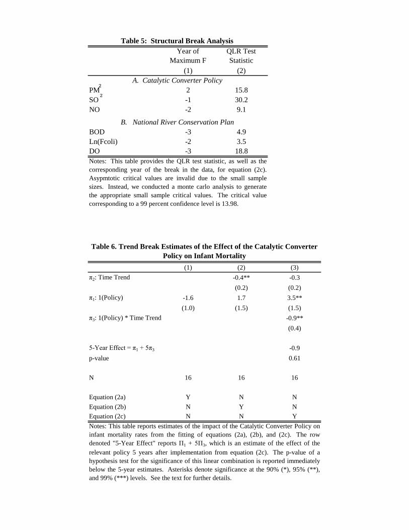
Year of
Maximum F
QLR Test
Statistic
(1) (2)
PM 2 15.8
SO
₂
-1 30.2
NO
₂
-2 9.1
BOD -3 4.9
Ln(Fcoli) -2 3.5
DO -3 18.8
(1) (2) (3)
π2: Time Trend -0.4** -0.3
(0.2) (0.2)
π1: 1(Policy) -1.6 1.7 3.5**
(1.0) (1.5) (1.5)
π3: 1(Policy) * Time Trend -0.9**
(0.4)
5-Year Effect = π1 + 5π3 -0.9
p-value 0.61
N 16 16 16
Equation (2a) Y N N
Equation (2b) N Y N
Equation (2c) N N Y
Notes: This table reports estimates of the impact of the Catalytic Converter Policy on
infant mortality rates from the fitting of equations (2a), (2b), and (2c). The row
denoted "5-Year Effect" reports Π1 + 5Π3, which is an estimate of the effect of the
relevant policy 5 years after implementation from equation (2c). The p-value of a
hypothesis test for the significance of this linear combination is reported immediately
below the 5-year estimates. Asterisks denote significance at the 90% (*), 95% (**),
and 99% (***) levels. See the text for further details.
B. National River Conservation Plan
Table 5: Structural Break Analysis
A. Catalytic Converter Policy
Notes: This table provides the QLR test statistic, as well as the
corresponding year of the break in the data, for equation (2c).
Asypmtotic critical values are invalid due to the small sample
sizes. Instead, we conducted a monte carlo analysis to generate
the appropriate small sample critical values. The critical value
corresponding to a 99 percent confidence level is 13.98.
Table 6. Trend Break Estimates of the Effect of the Catalytic Converter
Policy on Infant Mortality

High Low High Low High Low High Low
(1) (2) (3) (4) (5) (6) (7) (8)
Panel A: PM
5-Year Effect = π1 + 5π3 -57.9** -39.6 -42.8* -18.2 -38.5** -85.7* -61.5* -47.2**
p-value 0.04 0.20 0.08 0.61 0.05 0.06 0.06 0.04
Panel B: SO2
5-Year Effect -15.1*** -10.1*** -20.5*** 12.7*** -13.0*** -11.1 -6.2*** -19.4***
p-value 0.00 0.01 0.00 0.00 0.00 0.11 0.01 0.00
Panel C: NO2
5-Year Effect -1.9 -0.9 -4.2 4.5 0.4 -3.7 1.6 -5.3
p-value 0.76 0.85 0.31 0.51 0.93 0.68 0.80 0.31
Notes: This table explores the heterogeneity of the treatment effect for the Catalytic converter policy. We report estimates
from fitting equation (2c), our prefered specification. Asterisks denote significance at the 90% (*), 95% (**), and 99% (***)
levels.
Table 7: Heterogeneity of Effect of Catalytic Converter Policy
Urban Literacy
Air Pollution
Mentions Corruption Mentions
Transparency
International
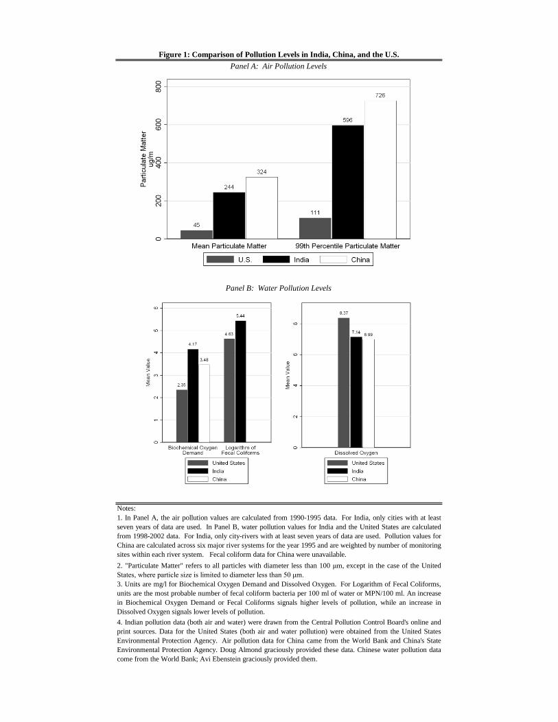
Notes:
1. In Panel A, the air pollution values are calculated from 1990-1995 data. For India, only cities with at least
seven years of data are used. In Panel B, water pollution values for India and the United States are calculated
from 1998-2002 data. For India, only city-rivers with at least seven years of data are used. Pollution values for
China are calculated across six major river systems for the year 1995 and are weighted by number of monitoring
sites within each river system. Fecal coliform data for China were unavailable.
2. "Particulate Matter" refers to all particles with diameter less than 100 μm, except in the case of the United
States, where particle size is limited to diameter less than 50 μm.
3. Units are mg/l for Biochemical Oxygen Demand and Dissolved Oxygen. For Logarithm of Fecal Coliforms,
units are the most probable number of fecal coliform bacteria per 100 ml of water or MPN/100 ml. An increase
in Biochemical Oxygen Demand or Fecal Coliforms signals higher levels of pollution, while an increase in
Dissolved Oxygen signals lower levels of pollution.
4. Indian pollution data (both air and water) were drawn from the Central Pollution Control Board's online and
print sources. Data for the United States (both air and water pollution) were obtained from the United States
Environmental Protection Agency. Air pollution data for China came from the World Bank and China's State
Environmental Protection Agency. Doug Almond graciously provided these data. Chinese water pollution data
come from the World Bank; Avi Ebenstein graciously provided them.
Figure 1: Comparison of Pollution Levels in India, China, and the U.S.
Panel A: Air Pollution Levels
Panel B: Water Pollution Levels

Notes:
Notes:
2. Geographical data are drawn from MIT's Geodata Repository. Monitoring locations
are determined from CPCB and SPCB online sources and Google Maps.
Figure 2: Air Quality Monitors Across India
1. Dots denote cities with monitoring stations under India's National Ambient Air
Quality Monitoring Programme (NAAQMP).
2. Geographical data are drawn from MIT's Geodata Repository. Monitoring locations
are determined from CPCB and SPCB online sources and Google Maps.
Figure 3: Water Quality Monitors on India's Major Rivers
1. Dots denote cities with monitoring stations under India's National Water Monitoring
Programme (NWMP). Only cities with monitors on major rivers are included, as
geospatial data for smaller rivers is unavailable.
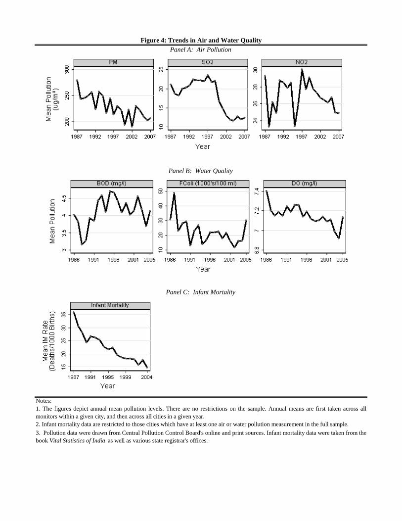
Notes:
3. Pollution data were drawn from Central Pollution Control Board's online and print sources. Infant mortality data were taken from the
book Vital Statistics of India as well as various state registrar's offices.
Figure 4: Trends in Air and Water Quality
Panel A: Air Pollution
Panel B: Water Quality
Panel C: Infant Mortality
1. The figures depict annual mean pollution levels. There are no restrictions on the sample. Annual means are first taken across all
monitors within a given city, and then across all cities in a given year.
2. Infant mortality data are restricted to those cities which have at least one air or water pollution measurement in the full sample.

Figure 5. Event Study of Air Pollution Policies
Panel A. PM Panel B. SO2 Panel C. NO2
Notes: The figures provide a graphical analysis of the effect of the Supreme Court Action Plans and mandated Catalytic Converter policies on air
pollution. The figures plot the estimated στ's against the τ's from the estimation of equation (1). Each pair of graphs within a panel are based on the same
regression. See the text for further details.
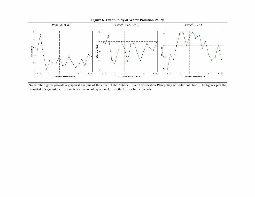
Notes: The figures provide a graphical analysis of the effect of the National River Conservation Plan policy on water pollution. The figures plot the
estimated στ's against the τ's from the estimation of equation (1). See the text for further details.
Figure 6. Event Study of Water Pollution Policy
Panel A. BOD Panel B. Ln(Fcoli) Panel C. DO
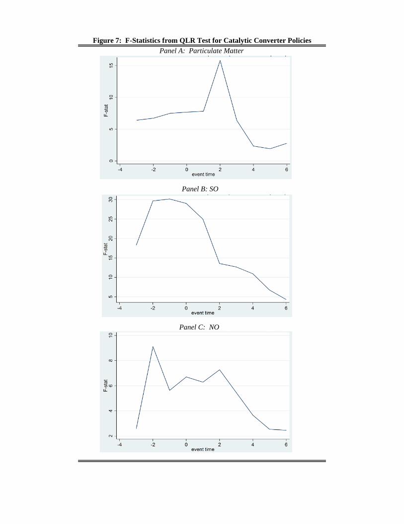
Figure 7: F-Statistics from QLR Test for Catalytic Converter Policies
Panel A: Particulate Matter
Panel B: SO
₂
Panel C: NO
₂

Source: Author Compilation from the Times of India
Figure 9: Total Nationwide References to Air and Water Pollution in Times of India, 1986 – 2007
334
109
0
100
200
300
400
Num
ber
of R
efe
rence
s
Air Pollution Water Pollution
01
02
03
04
05
06
0
Num
ber
of R
efe
rence
s
1986 1989 1992 1995 1998 2001 2004 2007Year
Air Pollution Water Pollution
Figure 8. Event Study of Catalytic Converters and Infant Mortality
Notes: The figure provides a graphical analysis of the effect of the Catalytic
Converter policy on the infant mortality rate. The figure plots the estimated στ's
against the τ's from the estimation of equation (1). See the text for further details.
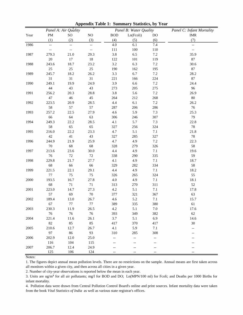
Panel C: Infant Mortality
Year PM SO
₂
NO
₂
BOD Ln(Fcoli) DO IMR
(1) (2) (3) (4) (5) (6) (7)
1986 -- -- -- 4.0 6.1 7.4 --
-- -- -- 111 100 110 --
1987 279.3 21.0 29.3 3.8 6.5 7.2 35.9
20 17 18 122 101 119 87
1988 243.6 18.7 23.2 3.2 6.3 7.2 30.6
25 25 25 190 162 195 87
1989 245.7 18.2 26.2 3.3 6.7 7.2 28.2
31 31 31 221 166 224 87
1990 249.1 19.9 24.9 3.9 6.6 7.2 24.4
44 43 43 273 205 275 96
1991 256.2 20.3 28.8 3.8 5.6 7.2 26.9
47 46 45 264 212 268 80
1992 223.5 20.9 28.5 4.4 6.1 7.2 26.2
58 57 57 287 206 286 76
1993 257.2 22.5 27.9 4.6 5.9 7.3 25.3
66 64 63 306 246 307 79
1994 249.3 22.2 28.5 4.1 5.7 7.3 22.8
58 65 65 327 256 324 78
1995 216.0 22.2 23.3 4.7 5.1 7.1 21.8
42 41 43 327 285 327 78
1996 244.9 21.9 25.9 4.7 4.9 7.2 22.3
70 68 68 328 279 326 58
1997 213.6 23.6 30.0 4.4 4.9 7.1 19.6
76 72 72 338 290 335 59
1998 229.8 21.7 27.7 4.1 4.9 7.1 18.7
68 66 66 329 282 334 58
1999 221.5 22.1 29.1 4.4 4.9 7.1 18.2
77 75 75 326 265 324 55
2000 193.5 16.7 27.8 4.0 4.9 7.1 18.1
68 71 71 313 270 311 52
2001 223.0 14.7 27.3 4.2 5.1 7.1 17.8
57 69 70 377 321 367 63
2002 189.4 13.0 26.7 4.6 5.2 7.1 15.7
67 77 77 389 335 380 61
2003 230.3 11.9 26.5 4.2 5.1 7.0 17.6
76 76 76 393 349 382 62
2004 221.4 11.6 26.1 3.7 5.1 6.9 14.6
82 85 85 417 370 417 30
2005 210.6 12.7 26.7 4.1 5.9 7.1 --
97 86 93 310 285 308 --
2006 202.9 12.0 25.0 -- -- -- --
116 104 115 -- -- -- --
2007 206.7 12.4 24.9 -- -- -- --
125 106 124 -- -- -- --
Notes:
4. Pollution data were drawn from Central Pollution Control Board's online and print sources. Infant mortality data were taken
from the book Vital Statistics of India as well as various state registrar's offices.
Appendix Table 1: Summary Statistics, by Year
Panel A: Air Quality Panel B: Water Quality
1. The figures depict annual mean pollution levels. There are no restrictions on the sample. Annual means are first taken across
all monitors within a given city, and then across all cities in a given year.
2. Number of city-year observations is reported below the mean in each year.
3. Units are ug/m³ for all air pollutants; mg/l for BOD and DO; Ln(MPN/100 ml) for Fcoli; and Deaths per 1000 Births for
infant mortality.

Water
Year
Supreme Court
Action Plans
Catalytic
Converters
National River
Conservation Plan
(1) (4) (6)
1986 -- -- 25
1987 0 0 25
1988 0 0 25
1989 0 0 25
1990 0 0 25
1991 0 0 25
1992 0 0 25
1993 0 0 25
1994 0 0 97
1995 0 0 160
1996 0 4 160
1997 0 4 160
1998 1 4 160
1999 1 49 160
2000 1 49 160
2001 1 49 160
2002 1 49 160
2003 12 49 160
2004 17 49 160
2005 17 49 160
2006 17 49 --
2007 17 49 --
Notes:
Appendix Table 2: Pollution Policy Coverage in India
1. This table describes the incidence of each policy across all of India.
2. Policy data were drawn from a variety of sources that are detailed
in the text.
Air
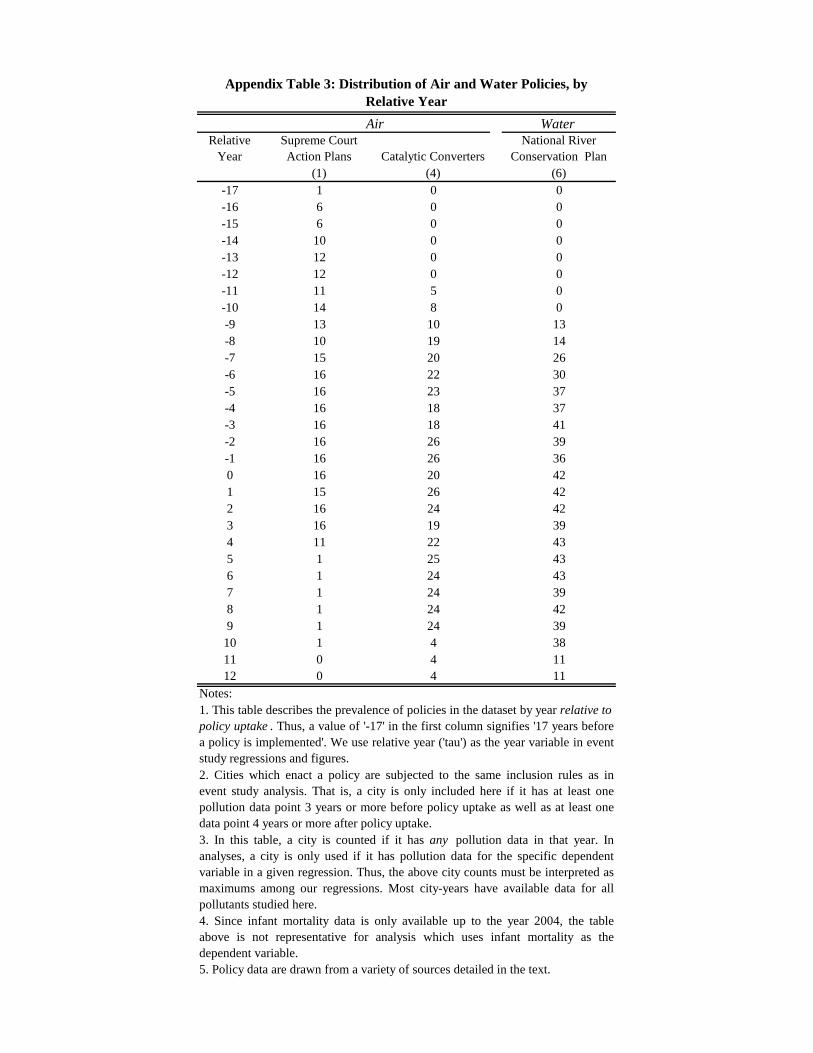
Water
Relative
Year
Supreme Court
Action Plans Catalytic Converters
National River
Conservation Plan
(1) (4) (6)
-17 1 0 0
-16 6 0 0
-15 6 0 0
-14 10 0 0
-13 12 0 0
-12 12 0 0
-11 11 5 0
-10 14 8 0
-9 13 10 13
-8 10 19 14
-7 15 20 26
-6 16 22 30
-5 16 23 37
-4 16 18 37
-3 16 18 41
-2 16 26 39
-1 16 26 36
0 16 20 42
1 15 26 42
2 16 24 42
3 16 19 39
4 11 22 43
5 1 25 43
6 1 24 43
7 1 24 39
8 1 24 42
9 1 24 39
10 1 4 38
11 0 4 11
12 0 4 11
Notes:
5. Policy data are drawn from a variety of sources detailed in the text.
Appendix Table 3: Distribution of Air and Water Policies, by
Relative Year
Air
1. This table describes the prevalence of policies in the dataset by year relative to
policy uptake . Thus, a value of '-17' in the first column signifies '17 years before
a policy is implemented'. We use relative year ('tau') as the year variable in event
study regressions and figures.
2. Cities which enact a policy are subjected to the same inclusion rules as in
event study analysis. That is, a city is only included here if it has at least one
pollution data point 3 years or more before policy uptake as well as at least one
data point 4 years or more after policy uptake.
3. In this table, a city is counted if it has any pollution data in that year. In
analyses, a city is only used if it has pollution data for the specific dependent
variable in a given regression. Thus, the above city counts must be interpreted as
maximums among our regressions. Most city-years have available data for all
pollutants studied here.
4. Since infant mortality data is only available up to the year 2004, the table
above is not representative for analysis which uses infant mortality as the
dependent variable.
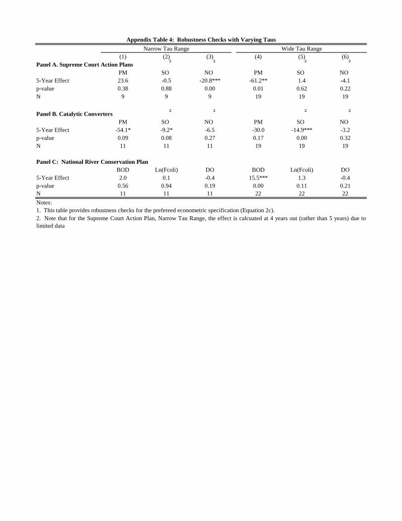
(1) (2) (3) (4) (5) (6)
PM SO
₂
NO
₂
PM SO
₂
NO
₂
5-Year Effect 23.6 -0.5 -20.8*** -61.2** 1.4 -4.1
p-value 0.38 0.88 0.00 0.01 0.62 0.22
N 9 9 9 19 19 19
PM SO
₂
NO
₂
PM SO
₂
NO
₂
5-Year Effect -54.1* -9.2* -6.5 -30.0 -14.9*** -3.2
p-value 0.09 0.08 0.27 0.17 0.00 0.32
N 11 11 11 19 19 19
BOD Ln(Fcoli) DO BOD Ln(Fcoli) DO
5-Year Effect 2.0 0.1 -0.4 15.5*** 1.3 -0.4
p-value 0.56 0.94 0.19 0.00 0.11 0.21
N 11 11 11 22 22 22
Notes:
1. This table provides robustness checks for the prefereed econometric specification (Equation 2c).
2. Note that for the Supreme Court Action Plan, Narrow Tau Range, the effect is calcuated at 4 years out (rather than 5 years) due to
limited data
Appendix Table 4: Robustness Checks with Varying Taus
Narrow Tau Range Wide Tau Range
Panel A. Supreme Court Action Plans
Panel B. Catalytic Converters
Panel C: National River Conservation Plan

Notes:
Appendix Figure 1A: Kernel Density Graphs of Air Quality
1. The graphs provide the distribution of air pollution for the early (1987-1990)
and later (2004-2007) periods of our sample. They are constructed using an
Epanechnikov kernel function.
2. Units are μg/m³ for all pollutants.
3. The data were drawn from Central Pollution Control Board's online and print
sources.
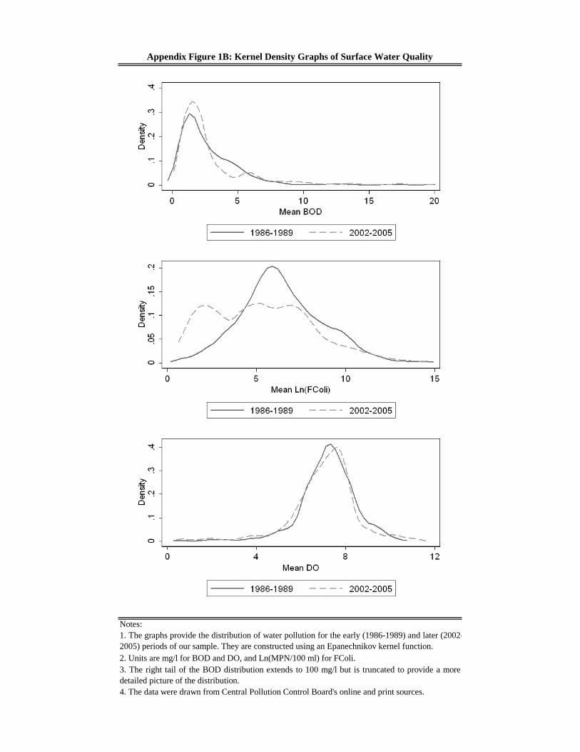
Notes:
Appendix Figure 1B: Kernel Density Graphs of Surface Water Quality
1. The graphs provide the distribution of water pollution for the early (1986-1989) and later (2002-
2005) periods of our sample. They are constructed using an Epanechnikov kernel function.
2. Units are mg/l for BOD and DO, and Ln(MPN/100 ml) for FColi.
3. The right tail of the BOD distribution extends to 100 mg/l but is truncated to provide a more
detailed picture of the distribution.
4. The data were drawn from Central Pollution Control Board's online and print sources.
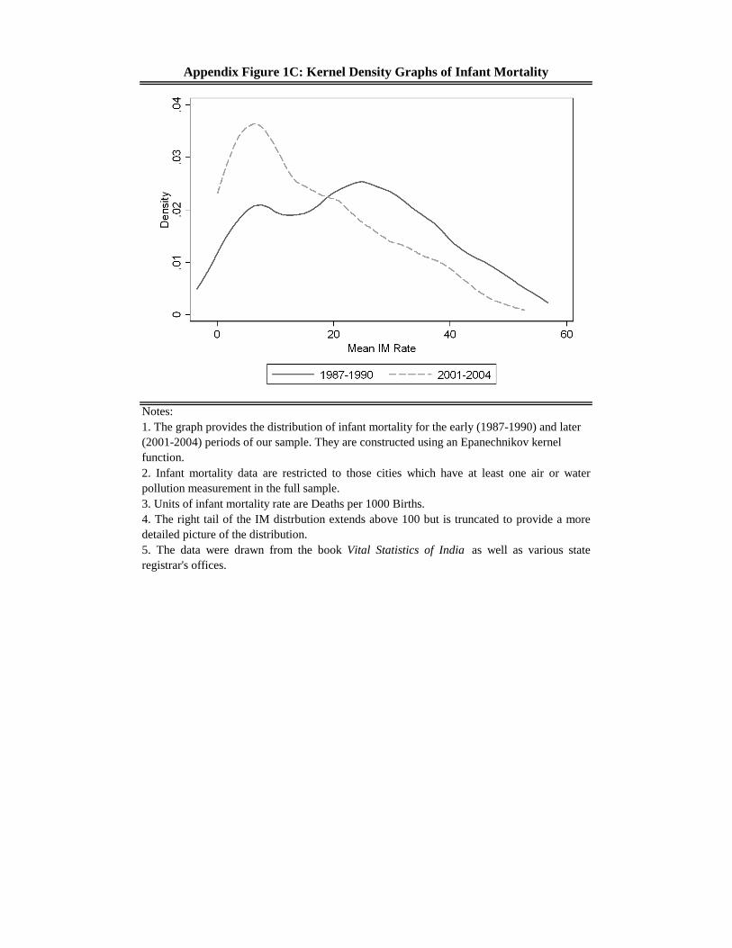
Notes:
5. The data were drawn from the book Vital Statistics of India as well as various state
registrar's offices.
Appendix Figure 1C: Kernel Density Graphs of Infant Mortality
1. The graph provides the distribution of infant mortality for the early (1987-1990) and later
(2001-2004) periods of our sample. They are constructed using an Epanechnikov kernel
function.
2. Infant mortality data are restricted to those cities which have at least one air or water
pollution measurement in the full sample.
3. Units of infant mortality rate are Deaths per 1000 Births.
4. The right tail of the IM distrbution extends above 100 but is truncated to provide a more
detailed picture of the distribution.