epa - montecarlo principle.pdf

7/29/2019 EPA - montecarlo principle.pdf

http://slidepdf.com/reader/full/epa-montecarlo-principlepdf 1/39

EPA/630/R-97/001

March 1997

Guiding Principles for Monte CarloAnalysis

Technical Panel

Office of Prevention, Pesticides, and Toxic Substances

Michael Firestone (Chair) Penelope Fenner-Crisp

Office of Policy, Planning, and Evaluation

Timothy Barry

Office of Solid Waste and Emergency Response

David Bennett Steven Chang

Office of Research and Development

Michael Callahan

Regional Offices

AnneMarie Burke (Region I) Jayne Michaud (Region I)

Marian Olsen (Region II) Patricia Cirone (Region X)

Science Advisory Board Staff

Donald Barnes

Risk Assessment Forum Staff

William P. Wood Steven M. Knott

Risk Assessment Forum

U.S. Environmental Protection Agency

Washington, DC 20460



ii

DISCLAIMER

This document has been reviewed in accordance with U.S. Environmental Protection

Agency policy and approved for publication. Mention of trade names or commercial products

does not constitute endorsement or recommendation for use.



iii

TABLE OF CONTENTS

Preface . . . . . . . . . . . . . . . . . . . . . . . . . . . . . . . . . . . . . . . . . . . . . . . . . . . . . . . . . . . . . . . . . . . iv

Introduction . . . . . . . . . . . . . . . . . . . . . . . . . . . . . . . . . . . . . . . . . . . . . . . . . . . . . . . . . . . . . . . 1

Fundamental Goals and Challenges . . . . . . . . . . . . . . . . . . . . . . . . . . . . . . . . . . . . . . . . . . . . . . 3

When a Monte Carlo Analysis Might Add Value to a Quantitative Risk Assessment . . . . . . . . . . 5

Key Terms and Their Definitions . . . . . . . . . . . . . . . . . . . . . . . . . . . . . . . . . . . . . . . . . . . . . . . 6

Preliminary Issues and Considerations . . . . . . . . . . . . . . . . . . . . . . . . . . . . . . . . . . . . . . . . . . . . 9

Defining the Assessment Questions . . . . . . . . . . . . . . . . . . . . . . . . . . . . . . . . . . . . . . . . 9

Selection and Development of the Conceptual and Mathematical Models . . . . . . . . . . . 10

Selection and Evaluation of Available Data . . . . . . . . . . . . . . . . . . . . . . . . . . . . . . . . . 10

Guiding Principles for Monte Carlo Analysis . . . . . . . . . . . . . . . . . . . . . . . . . . . . . . . . . . . . . . 11

Selecting Input Data and Distributions for Use in Monte Carlo Analysis . . . . . . . . . . . . 11

Evaluating Variability and Uncertainty . . . . . . . . . . . . . . . . . . . . . . . . . . . . . . . . . . . . . 15

Presenting the Results of a Monte Carlo Analysis . . . . . . . . . . . . . . . . . . . . . . . . . . . . . 17

Appendix: Probability Distribution Selection Issues . . . . . . . . . . . . . . . . . . . . . . . . . . . . . . . . . 22

References Cited in Text . . . . . . . . . . . . . . . . . . . . . . . . . . . . . . . . . . . . . . . . . . . . . . . . . . . . . 29



iv

PREFACE

The U.S. Environmental Protection Agency (EPA) Risk Assessment Forum was

established to promote scientific consensus on risk assessment issues and to ensure that this

consensus is incorporated into appropriate risk assessment guidance. To accomplish this, the Risk

Assessment Forum assembles experts throughout EPA in a formal process to study and report on

these issues from an Agency-wide perspective. For major risk assessment activities, the Risk

Assessment Forum has established Technical Panels to conduct scientific reviews and analyses.

Members are chosen to assure that necessary technical expertise is available.

This report is part of a continuing effort to develop guidance covering the use of

probabilistic techniques in Agency risk assessments. This report draws heavily on the

recommendations from a May 1996 workshop organized by the Risk Assessment Forum that

convened experts and practitioners in the use of Monte Carlo analysis, internal as well as externalto EPA, to discuss the issues and advance the development of guiding principles concerning how

to prepare or review an assessment based on use of Monte Carlo analysis. The conclusions and

recommendations that emerged from these discussions are summarized in the report “Summary

Report for the Workshop on Monte Carlo Analysis” (EPA/630/R-96/010). Subsequent to the

workshop, the Risk Assessment Forum organized a Technical Panel to consider the workshop

recommendations and to develop an initial set of principles to guide Agency risk assessors in the

use of probabilistic analysis tools including Monte Carlo analysis. It is anticipated that there will

be need for further expansion and revision of these guiding principles as Agency risk assessors

gain experience in their application.



1

Introduction

The importance of adequately characterizing variability and uncertainty in fate, transport,

exposure, and dose-response assessments for human health and ecological risk assessments has

been emphasized in several U.S. Environmental Protection Agency (EPA) documents and

activities. These include:

the 1986 Risk Assessment Guidelines;

the 1992 Risk Assessment Council (RAC) Guidance (the Habicht memorandum);

the 1992 Exposure Assessment Guidelines; and

the 1995 Policy for Risk Characterization (the Browner memorandum).

As a follow up to these activities EPA is issuing this policy and preliminary guidance on

using probabilistic analysis. The policy documents the EPA's position “that such probabilistic

analysis techniques as Monte Carlo analysis, given adequate supporting data and credible

assumptions, can be viable statistical tools for analyzing variability and uncertainty in risk

assessments.” The policy establishes conditions that are to be satisfied by risk assessments that

use probabilistic techniques. These conditions relate to the good scientific practices of clarity,

consistency, transparency, reproducibility, and the use of sound methods.

The EPA policy lists the following conditions for an acceptable risk assessment that uses

probabilistic analysis techniques. These conditions were derived from principles that are

presented later in this document and its Appendix. Therefore, after each condition, the relevant

principles are noted.

1. The purpose and scope of the assessment should be clearly articulated in a "problem

formulation" section that includes a full discussion of any highly exposed or highly

susceptible subpopulations evaluated (e.g., children, the elderly, etc.). The questions

the assessment attempts to answer are to be discussed and the assessment endpoints

are to be well defined.

2. The methods used for the analysis (including all models used, all data upon which the

assessment is based, and all assumptions that have a significant impact upon the

results) are to be documented and easily located in the report. This documentation is



2

to include a discussion of the degree to which the data used are representative of the

population under study. Also, this documentation is to include the names of the

models and software used to generate the analysis. Sufficient information is to be

provided to allow the results of the analysis to be independently reproduced.

(Principles 4, 5, 6, and 11)

3. The results of sensitivity analyses are to be presented and discussed in the report.

Probabilistic techniques should be applied to the compounds, pathways, and factors of

importance to the assessment, as determined by sensitivity analyses or other basic

requirements of the assessment. (Principles 1 and 2)

4. The presence or absence of moderate to strong correlations or dependencies between

the input variables is to be discussed and accounted for in the analysis, along with theeffects these have on the output distribution. (Principles 1 and 14)

5. Information for each input and output distribution is to be provided in the report. This

includes tabular and graphical representations of the distributions (e.g., probability

density function and cumulative distribution function plots) that indicate the location

of any point estimates of interest (e.g., mean, median, 95 percentile). The selectionth

of distributions is to be explained and justified. For both the input and output

distributions, variability and uncertainty are to be differentiated where possible.

(Principles 3, 7, 8, 10, 12, and 13)

6. The numerical stability of the central tendency and the higher end (i.e., tail) of the

output distributions are to be presented and discussed. (Principle 9)

7. Calculations of exposures and risks using deterministic (e.g., point estimate) methods

are to be reported if possible. Providing these values will allow comparisons between

the probabilistic analysis and past or screening level risk assessments. Further,

deterministic estimates may be used to answer scenario specific questions and to

facilitate risk communication. When comparisons are made, it is important to explain

the similarities and differences in the underlying data, assumptions, and models.

(Principle 15).



3

8. Since fixed exposure assumptions (e.g., exposure duration, body weight) are

sometimes embedded in the toxicity metrics (e.g., Reference Doses, Reference

Concentrations, unit cancer risk factors), the exposure estimates from the probabilistic

output distribution are to be aligned with the toxicity metric.

The following sections present a general framework and broad set of principles important

for ensuring good scientific practices in the use of Monte Carlo analysis (a frequently encountered

tool for evaluating uncertainty and variability). Many of the principles apply generally to the

various techniques for conducting quantitative analyses of variability and uncertainty; however,

the focus of the following principles is on Monte Carlo analysis. EPA recognizes that quantitative

risk assessment methods and quantitative variability and uncertainty analysis are undergoing rapid

development. These guiding principles are intended to serve as a minimum set of principles and

are not intended to constrain or prevent the use of new or innovative improvements wherescientifically defensible.

Fundamental Goals and Challenges

In the context of this policy, the basic goal of a Monte Carlo analysis is to chatacterize,

quantitatively, the uncertainty and variability in estimates of exposure or risk. A secondary goal is

to identify key sources of variability and uncertainty and to quantify the relative contribution of

these sources to the overall variance and range of model results.

Consistent with EPA principles and policies, an analysis of variability and uncertainty

should provide its audience with clear and concise information on the variability in individual

exposures and risks; it should provide information on population risk (extent of harm in the

exposed population); it should provide information on the distribution of exposures and risks to

highly exposed or highly susceptible populations; it should describe qualitatively and

quantitatively the scientific uncertainty in the models applied, the data utilized, and the specific

risk estimates that are used.

Ultimately, the most important aspect of a quantitative variability and uncertainty analysismay well be the process of interaction between the risk assessor, risk manager and other

interested parties that makes risk assessment into a dynamic rather than a static process.

Questions for the risk assessor and risk manager to consider at the initiation of a quantitative

variability and uncertainty analysis include:



4

Will the quantitative analysis of uncertainty and variability improve the risk

assessment?

What are the major sources of variability and uncertainty? How will variability

and uncertainty be kept separate in the analysis?

Are there time and resources to complete a complex analysis?

Does the project warrant this level of effort?

Will a quantitative estimate of uncertainty improve the decision? How will the

regulatory decision be affected by this variability and uncertainty analysis?

What types of skills and experience are needed to perform the analysis?

Have the weaknesses and strengths of the methods been evaluated?

How will the variability and uncertainty analysis be communicated to the public

and decision makers?

One of the most important challenges facing the risk assessor is to communicate,

effectively, the insights an analysis of variability and uncertainty provides. It is important for the

risk assessor to remember that insights will generally be qualitative in nature even though the

models they derive from are quantitative. Insights can include:

An appreciation of the overall degree of variability and uncertainty and theconfidence that can be placed in the analysis and its findings.

An understanding of the key sources of variability and key sources of uncertainty

and their impacts on the analysis.

An understanding of the critical assumptions and their importance to the analysis

and findings.

An understanding of the unimportant assumptions and why they are unimportant.

An understanding of the extent to which plausible alternative assumptions or models could affect any conclusions.

An understanding of key scientific controversies related to the assessment and a

sense of what difference they might make regarding the conclusions.



6

Key Terms and Their Definitions

The following section presents definitions for a number of key terms which are used

throughout this document.

Bayesian

The Bayesian or subjective view is that the probability of an event is the degree of belief

that a person has, given some state of knowledge, that the event will occur. In the classical or

frequentist view, the probability of an event is the frequency with which an event occurs given a

long sequence of identical and independent trials. In exposure assessment situations, directly

representative and complete data sets are rarely available; inferences in these situations are

inherently subjective. The decision as to the appropriateness of either approach (Bayesian or

Classical) is based on the available data and the extent of subjectivity deemed appropriate.

Correlation, Correlation Analysis

Correlation analysis is an investigation of the measure of statistical association among

random variables based on samples. Widely used measures include the linear correlation

coefficient (also called the product-moment correlation coefficient or Pearson’s correlation

coefficient ), and such non-parametric measures as Spearman rank-order correlation coefficient ,

and Kendall’s tau. When the data are nonlinear, non-parametric correlation is generally

considered to be more robust than linear correlation.

Cumulative Distribution Function (CDF)

The CDF is alternatively referred to in the literature as the distribution function,

cumulative frequency function, or the cumulative probability function. The cumulative

distribution function, F(x), expresses the probability the random variable X assumes a value less

than or equal to some value x, F(x) = Prob (X x). For continuous random variables, the

cumulative distribution function is obtained from the probability density function by integration, or

by summation in the case of discrete random variables.

Latin Hypercube Sampling

In Monte Carlo analysis, one of two sampling schemes are generally employed: simple

random sampling or Latin Hypercube sampling. Latin hypercube sampling may be viewed as a

stratified sampling scheme designed to ensure that the upper or lower ends of the distributions



7

used in the analysis are well represented. Latin hypercube sampling is considered to be more

efficient than simple random sampling, that is, it requires fewer simulations to produce the same

level of precision. Latin hypercube sampling is generally recommended over simple random

sampling when the model is complex or when time and resource constraints are an issue.

Monte Carlo Analysis, Monte Carlo Simulation

Monte Carlo Analysis is a computer-based method of analysis developed in the 1940's that

uses statistical sampling techniques in obtaining a probabilistic approximation to the solution of a

mathematical equation or model.

Parameter

Two distinct, but often confusing, definitions for parameter are used. In the first usage

(preferred), parameter refers to the constants characterizing the probability density function or cumulative distribution function of a random variable. For example, if the random variable W is

known to be normally distributed with mean µ and standard deviation , the characterizing

constants µ and are called parameters. In the second usage, parameter is defined as the

constants and independent variables which define a mathematical equation or model. For

example, in the equation Z = X + Y, the independent variables (X,Y) and the constants ( , )

are all parameters.

Probability Density Function (PDF)

The PDF is alternatively referred to in the literature as the probability function or the

frequency function. For continuous random variables, that is, the random variables which can

assume any value within some defined range (either finite or infinite), the probability density

function expresses the probability that the random variable falls within some very small interval.

For discrete random variables, that is, random variables which can only assume certain isolated or

fixed values, the term probability mass function (PMF) is preferred over the term probability

density function. PMF expresses the probability that the random variable takes on a specific

value.

Random Variable

A random variable is a quantity which can take on any number of values but whose exact

value cannot be known before a direct observation is made. For example, the outcome of the toss



8

of a pair of dice is a random variable, as is the height or weight of a person selected at random

from the New York City phone book.

Representativeness

Representativeness is the degree to which a sample is characteristic of the population for

which the samples are being used to make inferences.

Sensitivity, Sensitivity Analysis

Sensitivity generally refers to the variation in output of a mathematical model with respect

to changes in the values of the model’s input. A sensitivity analysis attempts to provide a ranking

of the model’s input assumptions with respect to their contribution to model output variability or

uncertainty. The difficulty of a sensitivity analysis increases when the underlying model is

nonlinear, nonmonotonic or when the input parameters range over several orders of magnitude.Many measures of sensitivity have been proposed. For example, the partial rank correlation

coefficient and standardized rank regression coefficient have been found to be useful. Scatter

plots of the output against each of the model inputs can be a very effective tool for identifying

sensitivities, especially when the relationships are nonlinear. For simple models or for screening

purposes, the sensitivity index can be helpful.

In a broader sense, sensitivity can refer to how conclusions may change if models, data, or

assessment assumptions are changed.

Simulation

In the context of Monte Carlo analysis, simulation is the process of approximating the

output of a model through repetitive random application of a model’s algorithm.



9

Uncertainty

Uncertainty refers to lack of knowledge about specific factors, parameters, or models.

For example, we may be uncertain about the mean concentration of a specific pollutant at a

contaminated site or we may be uncertain about a specific measure of uptake (e.g., 95th percentile

fish consumption rate among all adult males in the United States). Uncertainty includes parameter

uncertainty (measurement errors, sampling errors, systematic errors), model uncertainty

(uncertainty due to necessary simplification of real-world processes, mis-specification of the

model structure, model misuse, use of inappropriate surrogate variables), and scenario

uncertainty (descriptive errors, aggregation errors, errors in professional judgment, incomplete

analysis).

Variability

Variability refers to observed differences attributable to true heterogeneity or diversity in a population or exposure parameter. Sources of variability are the result of natural random

processes and stem from environmental, lifestyle, and genetic differences among humans.

Examples include human physiological variation (e.g., natural variation in bodyweight, height,

breathing rates, drinking water intake rates), weather variability, variation in soil types and

differences in contaminant concentrations in the environment. Variability is usually not reducible

by further measurement or study (but can be better characterized).

Preliminary Issues and Considerations

Defining the Assessment Questions

The critical first step in any exposure assessment is to develop a clear and unambiguous

statement of the purpose and scope of the assessment. A clear understanding of the purpose will

help to define and bound the analysis. Generally, the exposure assessment should be made as

simple as possible while still including all important sources of risk. Finding the optimum match

between the sophistication of the analysis and the assessment problem may be best achieved using

a “tiered approach” to the analysis, that is, starting as simply as possible and sequentially

employing increasingly sophisticated analyses, but only as warranted by the value added to the

analysis and decision process.



10

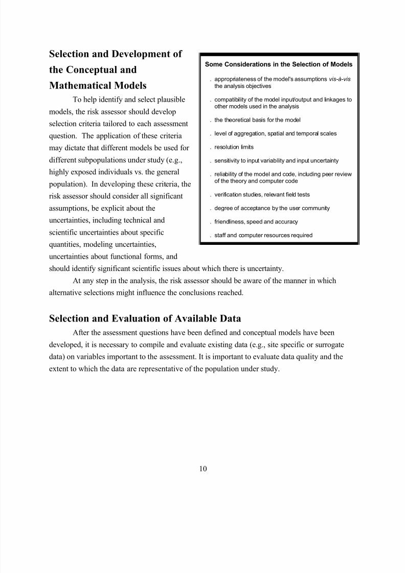
Some Considerations in the Selection of Models

. appropriateness of the model's assumptions vis-à-vis

the analysis objectives

. compatibility of the model input/output and linkages toother models used in the analysis

. the theoretical basis for the model

. level of aggregation, spatial and temporal scales

. resolution limits

. sensitivity to input variability and input uncertainty

. reliability of the model and code, including peer reviewof the theory and computer code

. verification studies, relevant field tests

. degree of acceptance by the user community

. friendliness, speed and accuracy

. staff and computer resources required

Selection and Development of

the Conceptual and

Mathematical Models

To help identify and select plausiblemodels, the risk assessor should develop

selection criteria tailored to each assessment

question. The application of these criteria

may dictate that different models be used for

different subpopulations under study (e.g.,

highly exposed individuals vs. the general

population). In developing these criteria, the

risk assessor should consider all significant

assumptions, be explicit about the

uncertainties, including technical and

scientific uncertainties about specific

quantities, modeling uncertainties,

uncertainties about functional forms, and

should identify significant scientific issues about which there is uncertainty.

At any step in the analysis, the risk assessor should be aware of the manner in which

alternative selections might influence the conclusions reached.

Selection and Evaluation of Available Data

After the assessment questions have been defined and conceptual models have been

developed, it is necessary to compile and evaluate existing data (e.g., site specific or surrogate

data) on variables important to the assessment. It is important to evaluate data quality and the

extent to which the data are representative of the population under study.



11

Guiding Principles for Monte Carlo Analysis

This section presents a discussion of principles of good practice for Monte Carlo

simulation as it may be applied to environmental assessments. It is not intended to serve as

detailed technical guidance on how to conduct or evaluate an analysis of variability and

uncertainty.

Selecting Input Data and Distributions for Use in Monte Carlo

Analysis

1. Conduct preliminary sensitivity analyses or numerical experiments to identify model

structures, exposure pathways, and model input assumptions and parameters that make

important contributions to the assessment endpoint and its overall variability and/or

uncertainty.The capabilities of current desktop computers allow for a number of "what if" scenarios to

be examined to provide insight into the effects on the analysis of selecting a particular model,

including or excluding specific exposure pathways, and making certain assumptions with respect

to model input parameters. The output of an analysis may be sensitive to the structure of the

exposure model. Alternative plausible models should be examined to determine if structural

differences have important effects on the output distribution (in both the region of central

tendency and in the tails).

Numerical experiments or sensitivity analysis also should be used to identify exposure

pathways that contribute significantly to or even dominate total exposure. Resources might be

saved by excluding unimportant exposure pathways (e.g., those that do not contribute appreciably

to the total exposure) from full probabilistic analyses or from further analyses altogether. For

important pathways, the model input parameters that contribute the most to overall variability and

uncertainty should be identified. Again, unimportant parameters may be excluded from full

probabilistic treatment. For important parameters, empirical distributions or parametric

distributions may be used. Once again, numerical experiments should be conducted to determine

the sensitivity of the output to different assumptions with respect to the distributional forms of

the input parameters. Identifying important pathways and parameters where assumptions about

distributional form contribute significantly to overall uncertainty may aid in focusing data

gathering efforts.



12

Dependencies or correlations between model parameters also may have a significant

influence on the outcome of the analysis. The sensitivity of the analysis to various assumptions

about known or suspected dependencies should be examined. Those dependencies or correlations

identified as having a significant effect must be accounted for in later analyses.

Conducting a systematic sensitivity study may not be a trivial undertaking, involving

significant effort on the part of the risk assessor. Risk assessors should exercise great care not to

prematurely or unjustifiably eliminate pathways or parameters from full probabilistic treatment.

Any parameter or pathway eliminated from full probabilistic treatment should be identified and the

reasons for its elimination thoroughly discussed.

2. Restrict the use of probabilistic assessment to significant pathways and parameters.

Although specifying distributions for all or most variables in a Monte Carlo analysis is

useful for exploring and characterizing the full range of variability and uncertainty, it is oftenunnecessary and not cost effective. If a systematic preliminary sensitivity analysis (that includes

examining the effects of various assumptions about distributions) was undertaken and

documented, and exposure pathways and parameters that contribute little to the assessment

endpoint and its overall uncertainty and variability were identified, the risk assessor may simplify

the Monte Carlo analysis by focusing on those pathways and parameters identified as significant.

From a computational standpoint, a Monte Carlo analysis can include a mix of point estimates and

distributions for the input parameters to the exposure model. However, the risk assessor and risk

manager should continually review the basis for "fixing" certain parameters as point values to

avoid the perception that these are indeed constants that are not subject to change.

3. Use data to inform the choice of input distributions for model parameters .

The choice of input distribution should always be based on all information (both

qualitative and quantitative) available for a parameter. In selecting a distributional form, the risk

assessor should consider the quality of the information in the database and ask a series of

questions including (but not limited to):

Is there any mechanistic basis for choosing a distributional family?

Is the shape of the distribution likely to be dictated by physical or biological

properties or other mechanisms?

Is the variable discrete or continuous?



13

What are the bounds of the variable?

Is the distribution skewed or symmetric?

If the distribution is thought to be skewed, in which direction?

What other aspects of the shape of the distribution are known?

When data for an important parameter are limited, it may be useful to define plausible

alternative scenarios to incorporate some information on the impact of that variable in the overall

assessment (as done in the sensitivity analysis). In doing this, the risk assessor should select the

widest distributional family consistent with the state of knowledge and should, for important

parameters, test the sensitivity of the findings and conclusions to changes in distributional shape.

4. Surrogate data can be used to develop distributions when they can be appropriately

justified.

The risk assessor should always seek representative data of the highest quality available.

However, the question of how representative the available data are is often a serious issue. Many

times, the available data do not represent conditions (e.g., temporal and spatial scales) in the

population being assessed. The assessor should identify and evaluate the factors that introduce

uncertainty into the assessment. In particular, attention should be given to potential biases that

may exist in surrogate data and their implications for the representativeness of the fitted

distributions.

When alternative surrogate data sets are available, care must be taken when selecting or

combining sets. The risk assessor should use accepted statistical practices and techniques when

combining data, consulting with the appropriate experts as needed.

Whenever possible, collect site or case specific data (even in limited quantities) to help

justify the use of the distribution based on surrogate data. The use of surrogate data to develop

distributions can be made more defensible when case-specific data are obtained to check the

reasonableness of the distribution.

5. When obtaining empirical data to develop input distributions for exposure model

parameters, the basic tenets of environmental sampling should be followed. Further,



According to NCRP (1996), an expert has (1) training and experience in the subject area resulting in1

superior knowledge in the field, (2) access to relevant information, (3) an ability to process and effectively use the

information, and (4) is recognized by his or her peers or those conducting the study as qualified to provide judgments

about assumptions, models, and model parameters at the level of detail required.

14

particular attention should be given to the quality of information at the tails of the

distribution.

As a general rule, the development of data for use in distributions should be carried out

using the basic principles employed for exposure assessments. For example,

Receptor-based sampling in which data are obtained on the receptor or on the

exposure fields relative to the receptor;

Sampling at appropriate spatial or temporal scales using an appropriate

stratified random sampling methodology;

Using two-stage sampling to determine and evaluate the degree of error,

statistical power, and subsequent sampling needs; and

Establishing data quality objectives.

In addition, the quality of information at the tails of input distributions often is not as good

as the central values. The assessor should pay particular attention to this issue when devising data

collection strategies.

6. Depending on the objectives of the assessment, expert judgment can be included either1

within the computational analysis by developing distributions using various methods or

by using judgments to select and separately analyze alternate, but plausible, scenarios.

When expert judgment is employed, the analyst should be very explicit about its use.Expert judgment is used, to some extent, throughout all exposure assessments. However,

debatable issues arise when applying expert opinions to input distributions for Monte Carlo

analyses. Using expert judgment to derive a distribution for an input parameter can reflect bounds

on the state of knowledge and provide insights into the overall uncertainty. This may be

particularly useful during the sensitivity analysis to help identify important variables for which

additional data may be needed. However, distributions based exclusively or primarily on expert

judgment reflect the opinion of individuals or groups and, therefore, may be subject to

considerable bias. Further, without explicit documentation of the use of expert opinions, the



15

distributions based on these judgments might be erroneously viewed as equivalent to those based

on hard data. When distributions based on expert judgement have an appreciable effect on the

outcome of an analysis, it is critical to highlight this in the uncertainty characterization.

Evaluating Variability and Uncertainty7. The concepts of variability and uncertainty are distinct. They can be tracked and

evaluated separately during an analysis, or they can be analyzed within the same

computational framework. Separating variability and uncertainty is necessary to

provide greater accountability and transparency. The decision about how to track

them separately must be made on a case-by-case basis for each variable.

Variability represents the true heterogeneity or diversity inherent in a well-characterized

population. As such, it is not reducible through further study. Uncertainty represents a lack of

knowledge about the population. It is sometimes reducible through further study. Therefore,

separating variability and uncertainty during the analysis is necessary to identify parameters for

which additional data are needed. There can be uncertainty about the variability within a

population. For example, if only a subset of the population is measured or if the population is

otherwise under-sampled, the resulting measure of variability may differ from the true population

variability. This situation may also indicate the need for additional data collection.

8. There are methodological differences regarding how variability and uncertainty are

addressed in a Monte Carlo analysis.There are formal approaches for distinguishing between and evaluating variability and

uncertainty. When deciding on methods for evaluating variability and uncertainty, the assessor

should consider the following issues.

Variability depends on the averaging time, averaging space, or other dimensions

in which the data are aggregated.

Standard data analysis tends to understate uncertainty by focusing solely on

random error within a data set. Conversely, standard data analysis tends to

overstate variability by implicitly including measurement errors.

Various types of model errors can represent important sources of uncertainty.

Alternative conceptual or mathematical models are a potentially important source

of uncertainty. A major threat to the accuracy of a variability analysis is a lack of

representativeness of the data.



16

9. Methods should investigate the numerical stability of the moments and the tails of the

distributions.

For the purposes of these principles, numerical stability refers to observed numerical

changes in the characteristics (i.e., mean, variance, percentiles) of the Monte Carlo simulationoutput distribution as the number of simulations increases. Depending on the algebraic structure

of the model and the exact distributional forms used to characterize the input parameters, some

outputs will stabilize quickly, that is, the output mean and variance tend to reach more or less

constant values after relatively few sampling iterations and exhibit only relatively minor

fluctuations as the number of simulations increases. On the other hand, some model outputs may

take longer to stabilize. The risk assessor should take care to be aware of these behaviors. Risk

assessors should always use more simulations than they think necessary. Ideally, Monte Carlo

simulations should be repeated using several non-overlapping subsequences to check for stability

and repeatability. Random number seeds should always be recorded. In cases where the tails of

the output distribution do not stabilize, the assessor should consider the quality of information in

the tails of the input distributions. Typically, the analyst has the least information about the input

tails. This suggest two points.

Data gathering efforts should be structured to provide adequate coverage at the

tails of the input distributions.

The assessment should include a narrative and qualitative discussion of the

quality of information at the tails of the input distributions.

10. There are limits to the assessor's ability to account for and characterize all sources of

uncertainty. The analyst should identify areas of uncertainty and include them in the

analysis, either quantitatively or qualitatively.

Accounting for the important sources of uncertainty should be a key objective in Monte

Carlo analysis. However, it is not possible to characterize all the uncertainties associated with the

models and data. The analyst should attempt to identify the full range of types of uncertainty

impinging on an analysis and clearly disclose what set of uncertainties the analysis attempts to

represent and what it does not. Qualitative evaluations of uncertainty including relative ranking of

the sources of uncertainty may be an acceptable approach to uncertainty evaluation, especially

when objective quantitative measures are not available. Bayesian methods may sometimes be



17

useful for incorporating subjective information into variability and uncertainty analyses in a

manner that is consistent with distinguishing variability from uncertainty.

Presenting the Results of a Monte Carlo Analysis

11. Provide a complete and thorough description of the exposure model and its equations

(including a discussion of the limitations of the methods and the results).

Consistent with the Exposure Assessment Guidelines, Model Selection Guidance, and

other relevant Agency guidance, provide a detailed discussion of the exposure model(s) and

pathways selected to address specific assessment endpoints. Show all the formulas used. Define

all terms. Provide complete references. If external modeling was necessary (e.g., fate and

transport modeling used to provide estimates of the distribution of environmental concentrations),

identify the model (including version) and its input parameters. Qualitatively describe the major

advantages and limitations of the models used.The objectives are transparency and reproducibility - to provide a complete enough

description so that the assessment might be independently duplicated and verified.

12. Provide detailed information on the input distributions selected. This information

should identify whether the input represents largely variability, largely uncertainty,

or some combination of both. Further, information on goodness-of-fit statistics

should be discussed.

It is important to document thoroughly and convey critical data and methods that providean important context for understanding and interpreting the results of the assessment. This

detailed information should distinguish between variability and uncertainty and should include

graphs and charts to visually convey written information.

The probability density function (PDF) and cumulative distribution function (CDF) graphs

provide different, but equally important insights. A plot of a PDF shows possible values of a

random variable on the horizontal axis and their respective probabilities (technically, their

densities) on the vertical axis. This plot is useful for displaying:

the relative probability of values;

the most likely values (e.g., modes);

the shape of the distribution (e.g., skewness, kurtosis); and



18

small changes in probability density.

A plot of the cumulative distribution function shows the probability that the value of a random

variable is less than a specific value. These plots are good for displaying:

fractiles, including the median;

probability intervals, including confidence intervals;

stochastic dominance; and

mixed, continuous, and discrete distributions.

Goodness-of-fit tests are formal statistical tests of the hypothesis that a specific set of

sampled observations are an independent sample from the assumed distribution. Common tests

include the chi-square test, the Kolmogorov-Smirnov test, and the Anderson-Darling test.

Goodness-of-fit tests for normality and lognormality include Lilliefors' test, the Shapiro-Wilks'

test, and D'Agostino's test.

Risk assessors should never depend solely on the results of goodness-of-fit tests to select

the analytic form for a distribution. Goodness-of-fit tests have low discriminatory power and are

generally best for rejecting poor distribution fits rather than for identifying good fits. For small to

medium sample sizes, goodness-of-fit tests are not very sensitive to small differences between the

observed and fitted distributions. On the other hand, for large data sets, even small andunimportant differences between the observed and fitted distributions may lead to rejection of the

null hypothesis. For small to medium sample sizes, goodness-of-fit tests should best be viewed as

a systematic approach to detecting gross differences. The risk assessor should never let

differences in goodness-of-fit test results be the sole factor for determining the analytic form of a

distribution.

Graphical methods for assessing fit provide visual comparisons between the experimental

data and the fitted distribution. Despite the fact that they are non-quantitative, graphical methods

often can be most persuasive in supporting the selection of a particular distribution or in rejecting

the fit of a distribution. This persuasive power derives from the inherent weaknesses in numerical

goodness-of-fit tests. Such graphical methods as probability-probability (P-P) and quantile-

quantile (Q-Q) plots can provide clear and intuitive indications of goodness-of-fit.



19

Having selected and justified the selection of specific distributions, the assessor should

provide plots of both the PDF and CDF, with one above the other on the same page and using

identical horizontal scales. The location of the mean should be clearly indicated on both curves

[See Figure 1]. These graphs should be accompanied by a summary table of the relevant data.

13. Provide detailed information and graphs for each output distribution.

In a fashion similar to that for the input distributions, the risk assessor should provide

plots of both the PDF and CDF for each output distribution, with one above the other on the

same page, using identical horizontal scales. The location of the mean should clearly be indicated

on both curves. Graphs should be accompanied by a summary table of the relevant data.

14. Discuss the presence or absence of dependencies and correlations.

Covariance among the input variables can significantly affect the analysis output. It isimportant to consider covariance among the model's most sensitive variables. It is particularly

important to consider covariance when the focus of the analysis is on the high end (i.e., upper

end) of the distribution.

When covariance among specific parameters is suspected but cannot be determined due to

lack of data, the sensitivity of the findings to a range of different assumed dependencies should be

evaluated and reported.

15. Calculate and present point estimates.

Traditional deterministic (point) estimates should be calculated using established

protocols. Clearly identify the mathematical model used as well as the values used for each input

parameter in this calculation. Indicate in the discussion (and graphically) where the point estimate

falls on the distribution generated by the Monte Carlo analysis. Discuss the model and parameter

assumptions that have the most influence on the point estimate's position in the distribution. The

most important issue in comparing point estimates and Monte Carlo results is whether the data

and exposure methods employed in the two are comparable. Usually, when a major difference

between point estimates and Monte Carlo results is observed, there has been a fundamental

change in data or methods. Comparisons need to call attention to such differences and determine

their impact.

In some cases, additional point estimates could be calculated to address specific risk

management questions or to meet the information needs of the audience for the assessment. Point

estimates can often assist in communicating assessment results to certain groups by providing a



20

scenario-based perspective. For example, if point estimates are prepared for scenarios with which

the audience can identify, the significance of presented distributions may become clearer. This

may also be a way to help the audience identify important risks.

16. A tiered presentation style, in which briefing materials are assembled at various levels

of detail, may be helpful. Presentations should be tailored to address the questions

and information needs of the audience.

Entirely different types of reports are needed for scientific and nonscientific audiences.

Scientists generally will want more detail than non-scientists. Risk managers may need more

detail than the public. Reports for the scientific community are usually very detailed. Descriptive,

less detailed summary presentations and key statistics with their uncertainty intervals (e.g., box

and whisker plots) are generally more appropriate for non-scientists.

To handle the different levels of sophistication and detail needed for different audiences, itmay be useful to design a presentation in a tiered format where the level of detail increases with

each successive tier. For example, the first tier could be a one-page summary that might include a

graph or other numerical presentation as well as a couple of paragraphs outlining what was done.

This tier alone might be sufficient for some audiences. The next tier could be an executive

summary, and the third tier could be a full detailed report. For further information consult Bloom

et al., 1993.

Graphical techniques can play an indispensable role in communicating the findings from a

Monte Carlo analysis. It is important that the risk assessor select a clear and uncluttered graphical

style in an easily understood format. Equally important is deciding which information to display.

Displaying too much data or inappropriate data will weaken the effectiveness of the effort.

Having decided which information to display, the risk assessor should carefully tailor a graphical

presentation to the informational needs and sophistication of specific audiences. The performance

of a graphical display of quantitative information depends on the information the risk assessor is

trying to convey to the audience and on how well the graph is constructed (Cleveland, 1994). The

following are some recommendations that may prove useful for effective graphic presentation:

• Avoid excessively complicated graphs. Keep graphs intended for a glance (e.g.,overhead or slide presentations) relatively simple and uncluttered. Graphs

intended for publication can include more complexity.

• Avoid pie charts, perspective charts (3-dimensional bar and pie charts, ribbon

charts), pseudo-perspective charts (2-dimensional bar or line charts).



21

• Color and shading can create visual biases and are very difficult to use effectively.

Use color or shading only when necessary and then, only very carefully. Consult

references on the use of color and shading in graphics.

• When possible in publications and reports, graphs should be accompanied by a

table of the relevant data.

• If probability density or cumulative probability plots are presented, present both,

with one above the other on the same page, with identical horizontal scales and

with the location of the mean clearly indicated on both curves with a solid point.

• Do not depend on the audience to correctly interpret any visual display of data.

Always provide a narrative in the report interpreting the important aspects of the

graph.

• Descriptive statistics and box plots generally serve the less technically-oriented

audience well. Probability density and cumulative probability plots are generallymore meaningful to risk assessors and uncertainty analysts.



22

Appendix: Probability Distribution Selection Issues

Surrogate Data, Fitting Distributions, Default Distributions

Subjective DistributionsIdentification of relevant and valid data to represent an exposure variable is prerequisite to

selecting a probability distribution However, often the data available are not a direct measure of

the exposure variable of interest. The risk assessor is often faced with using data taken in spatial

or temporal scales that are significantly different from the scale of the problem under

consideration. The question becomes whether or not or how to use marginally representative or

surrogate data to represent a particular exposure variable. While there can be no hard and fast

rules on how to make that judgment, there are a number of questions risk assessors need to ask

when the surrogate data are the only data available.

I s there Prior Knowledge about M echanisms? Ideally, the selection of candidate probability

distributions should be based on consideration of the underlying physical processes or mechanismsthought to be key in giving rise to the observed variability. For example, if the exposure variable

is the result of the product of a large number of other random variables, it would make sense to

select a lognormal distribution for testing. As another example, the exponential distribution

would be a reasonable candidate if the stochastic variable represents a process akin to inter-arrival

times of events that occur at a constant rate. As a final example, a gamma distribution would be a

reasonable candidate if the random variable of interest was the sum of independent exponential

random variables.

Threshold Question - Are the sur rogate data of acceptable qual ity and representativeness to

suppor t r eli able exposur e estimates?

What uncertain ties and biases are li kely to be in troduced by using sur rogate data? For

example, if the data have been collected in a different geographic region, the contribution of

factors such as soil type, rainfall, ambient temperature, growing season, natural sources of

exposure, population density, and local industry may have a significant effect on the exposure

concentrations and activity patterns. If the data are collected from volunteers or from hot spots,

they will probably not represent the distribution of values in the population of interest. Each

difference between the survey data and the population being assessed should be noted. The

effects of these differences on the desired distribution should be discussed if possible.

How are the biases li kely to af fect the analysis and can the biases be corr ected? The risk

assessor may be able to state with a high degree of certainty that the available data over-estimatesor under-estimates the parameter of interest. Use of ambient air data on arsenic collected near

smelters will almost certainly over-estimate average arsenic exposures in the United States.

However, the smelter data can probably be used to produce an estimate of inhalation exposures

that falls within the high end. In other cases, the assessor may be unsure how unrepresentative

data will affect the estimate as in the case when data collected by a particular State are used in a



23

national assessment. In most cases, correction of suspected biases will be difficult or not possible.

If only hot spot data are available for example, only bounding or high end estimates may be

possible. Unsupported assumptions about biases should be avoided. Information regarding the

direction and extent of biases should be included in the uncertainty analysis.

How should any uncertainty introduced by the sur rogate data be represented?

In identifying plausible distributions to represent variability, the risk assessor should examine

the following characteristics of the variable:

1. Nature of the variable.

Can the variable only take on discrete values (e.g., either on or off; either heads or tails) or is

the variable continuous over some range (e.g., pollutant concentration; body weight; drinking

water consumption rate)? Is the variable correlated with or dependent on another variable?

2. Bounds of the variable.

What is the physical or plausible range of the variable (e.g., takes on only positive values; bounded by the interval [a,b]). Are physical measurements of the variable censored due to limits

of detection or some aspect of the experimental design?

3. Symmetry of the Di stri bution.

Is distribution of the variable known to be or thought to be skewed or symmetric? If the

distribution is thought to be skewed, in which direction? What other aspects of the shape of the

distribution are known? Is the shape of the distribution likely to be dictated by physical/biological

properties (e.g., logistic growth rates) or other mechanisms?

4. Summary Statistics .

Summary statistics can sometimes be useful in discriminating among candidate distributions.For example, frequently the range of the variable can be used to eliminate inappropriate

distributions; it would not be reasonable to select a lognormal distribution for an absorption

coefficient since the range of the lognormal distribution is (0, ) while the range of the absorption

coefficient is (0,1). If the coefficient of variation is near 1.0, then an exponential distribution

might be appropriate. Information on skewness can also be useful. For symmetric distributions,

skewness = 0; for distributions skewed to the right, skewness > 0; for distributions skewed to the

left, skewness < 0.

5. Graphi cal Methods to Explore the Data.

The risk assessor can often gain important insights by using a number of simple graphical

techniques to explore the data prior to numerical analysis. A wide variety of graphical methods

have been developed to aid in this exploration including frequency histograms for continuous

distributions, stem and leaf plots, dot plots, line plots for discrete distributions, box and whisker

plots, scatter plots, star representations, glyphs, Chernoff faces, etc. [Tukey (1977); Conover

(1980); du Toit et al. (1986); Morgan and Henrion, (1990)]. These graphical methods are all



24

intended to permit visual inspection of the density function corresponding to the distribution of

the data. They can assist the assessor in examining the data for skewness, behavior in the tails,

rounding biases, presence of multi-modal behavior, and data outliers.

Frequency histograms can be compared to the fundamental shapes associated with standard

analytic distributions (e.g., normal, lognormal, gamma, Weibull). Law and Kelton (1991) andEvans et al. (1993) have prepared a useful set of figures which plot many of the standard analytic

distributions for a range of parameter values. Frequency histograms should be plotted on both

linear and logarithmic scales and plotted over a range of frequency bin widths (class intervals) to

avoid too much jaggedness or too much smoothing (i.e., too little or too much data aggregation).

The data can be sorted and plotted on probability paper to check for normality (or log-normality).

Most of the statistical packages available for personal computers include histogram and

probability plotting features, as do most of the spreadsheet programs. Some statistical packages

include stem and leaf, and box and whisker plotting features.

After having explored the above characteristics of the variable, the risk assessor has three

basic techniques for representing the data in the analysis. In the first method, the assessor canattempt to fit a theoretical or parametric distribution to the data using standard statistical

techniques. As a second option, the assessor can use the data to define an empirical distribution

function (EDF). Finally, the assessor can use the data directly in the analysis utilizing random

resampling techniques (i.e., bootstrapping). Each of these three techniques has its own benefits.

However, there is no consensus among researchers (authors) as to which method is generally

superior. For example, Law and Kelton (1991) observe that EDFs may contain irregularities,

especially when the data are limited and that when an EDF is used in the typical manner, values

outside the range of the observed data cannot be generated. Consequently, when the data are

representative of the exposure variable and the fit is good, some prefer to use parametric

distributions. On the other hand, some authors prefer EDFs (Bratley, Fox and Schrage, 1987)

arguing that the smoothing which necessarily takes place in the fitting process distorts realinformation. In addition, when data are limited, accurate estimation of the upper end (tail) is

difficult. Ultimately, the technique selected will be a matter of the risk assessor’s comfort with the

techniques and the quality and quantity of the data under evaluation.

The following discussion focuses primarily on parametric techniques. For a discussion of the

other methods, the reader is referred to Efron and Tibshirani (1993), Law & Kelton (1991), and

Bratley et al (1987).

Having selected parametric distributions, it is necessary to estimate numerical values for the

intrinsic parameters which characterize each of the analytic distributions and assess the quality of

the resulting fit.

Parameter Estimation. Parameter estimation is generally accomplished using conventional

statistical methods, the most popular of which include the method of maximum likelihood,

method of least squares, and the method of moments. See Johnson and Kotz (1970), Law and



25

Kelton (1991), Kendall and Stewart (1979), Evans et al. (1993), Ang and Tang (1975),

Gilbert (1987), and Meyer (1975).

Assessing the Representativeness of the F itted Distr ibuti on. Having estimated the

parameters of the candidate distributions, it is necessary to evaluate the "quality of the fit"

and, if more than one distribution was selected, to select the "best" distribution from amongthe candidates. Unfortunately, there is no single, unambiguous measure of what constitutes

best fit. Ultimately, the risk assessor must judge whether or not the fit is acceptable.

Graphi cal M ethods for Assessing F it. Graphical methods provide visual comparisons

between the experimental data and the fitted distribution. Despite the fact that they are non-

quantitative, graphical methods often can be most persuasive in supporting the selection of a

particular distribution or in rejecting the fit of a distribution. This persuasive power derives

from the inherent weaknesses in numerical goodness-of-fit tests. Commonly used graphical

methods include: frequency comparisons which compare a histogram of the experimental data

with the density function of the fitted data; probability plots compare the observed cumulative

density function with the fitted cumulative density function. Probability plots are often based

on graphical transformations such that the plotted cumulative density function results in a

straight line; probability-probability plots (P-P plots) compare the observed probability with

the fitted probability. P-P plots tend to emphasize differences in the middle of the predicted

and observed cumulative distributions; quantile-quantile plots (Q-Q plots) graph the ith-

quantile of the fitted distribution against the ith quantile data. Q-Q plots tend to emphasize

differences in the tails of the fitted and observed cumulative distributions; and box plots

compare a box plot of the observed data with a box plot of the fitted distribution.

Goodness-of-F it Tests. Goodness-of-fit tests are formal statistical tests of the hypothesis that

the set of sampled observations are an independent sample from the assumed distribution.The null hypothesis is that the randomly sampled set of observations are independent,

identically distributed random variables with distribution function F. Commonly used

goodness-of-fit tests include the chi-square test, Kolmogorov-Smirnov test, and Anderson-

Darling test. The chi-square test is based on the difference between the square of the

observed and expected frequencies. It is highly dependent on the width and number of

intervals chosen and is considered to have low power. It is best used to reject poor fits. The

Kolmogorov-Smirnov Test is a non-parametric test based on the maximum absolute

difference between the theoretical and sample Cumulative Distribution Functions (CDFs).

The Kolmogorov-Smirnov test is most sensitive around the median and less sensitive in the

tails and is best at detecting shifts in the empirical CDF relative to the known CDF. It is less

proficient at detecting spread but is considered to be more powerful than the chi-square test.The Anderson-Darling test is designed to test goodness-of-fit in the tails of a Probability

Density Function (PDF) based on a weighted-average of the squared difference between the

observed and expected cumulative densities.



26

Care must be taken not to over-interpret or over-rely on the findings of goodness-of-fit tests.

It is far too tempting to use the power and speed of computers to run goodness-of-fit tests

against a generous list of candidate distributions, pick the distribution with the "best"

goodness-of-fit statistic, and claim that the distribution that fit "best" was not rejected at some

specific level of significance. This practice is statistically incorrect and should be avoided

[Bratley et al., 1987, page 134]. Goodness-of-fit tests have notoriously low power and aregenerally best for rejecting poor distribution fits rather than for identifying good fits. For

small to medium sample sizes, goodness-of-fit tests are not very sensitive to small differences

between the observed and fitted distributions. On the other hand, for large data sets, even

minute differences between the observed and fitted distributions may lead to rejection of the

null hypothesis. For small to medium sample sizes, goodness-of-fit tests should best be

viewed as a systematic approach to detecting gross differences.

Tests of Choice for Normali ty and Lognormality. Several tests for normality (and

lognormality when log-transformed data are used) which are considered more powerful than

either the chi-square or Komolgarov-Smirnoff (K-S) tests have been developed: Lilliefors'

test which is based on the K-S test but with "normalized" data values, Shapiro-Wilks test (for sample sizes 50), and D'Agostino's test (for sample sizes 50). The Shapiro-Wilks and

D'Agostino tests are the tests of choice when testing for normality or lognormality.

If the data are not well-fit by a theoretical distribution, the risk assessor should consider the

Empirical Distribution Function or bootstrapping techniques mentioned above.

For those situations in which the data are not adequately representative of the exposure

variable or where the quality or quantity of the data are questionable the following approaches

may be considered.

Distr ibuti ons Based on Surrogate Data. Production of an exposure assessment oftenrequires that dozens of factors be evaluated, including exposure concentrations, intake rates,

exposure times, and frequencies. A combination of monitoring, survey, and experimental

data, fate and transport modeling, and professional judgment is used to evaluate these factors.

Often the only available data are not completely representative of the population being

assessed. Some examples are the use of activity pattern data collected in one geographic

region to evaluate the duration of activities at a Superfund site in another region; use of

national intake data on consumption of a particular food item to estimate regional intake; and

use of data collected from volunteers to represent the general population.

In each such case, the question of whether to use the unrepresentative data to estimate the

distribution of a variable should be carefully evaluated. Considerations include how to express

the possible bias and uncertainty introduced by the unrepresentativeness of the data and

alternatives to using the data. In these situations, the risk assessor should carefully evaluate

the basis of the distribution (e.g., data used, method) before choosing a particular surrogate or

before picking among alternative distributions for the same exposure parameter. The



27

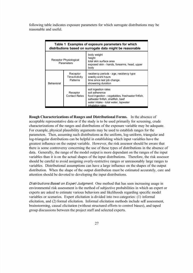
following table indicates exposure parameters for which surrogate distributions may be

reasonable and useful.

Table 1 Examples of exposure parameters for which

distributions based on surrogate data might be reasonable

Receptor PhysiologicalParameters

body weightheighttotal skin surface areaexposed skin - hands, forearms, head, upper body

Behavioral showering duration

Receptor residency periods - age, residency typeTime-Activity weekly work hours

Patterns time since last job change

Receptor soil adherence

Contact Rates food ingestion - vegetables, freshwater finfish,

soil ingestion rates

saltwater finfish, shellfish, beef water intake - total water, tapwater inhalation rates

Rough Characterizations of Ranges and Distributional Forms. In the absence of

acceptable representative data or if the study is to be used primarily for screening, crude

characterizations of the ranges and distributions of the exposure variable may be adequate.

For example, physical plausibility arguments may be used to establish ranges for the

parameters. Then, assuming such distributions as the uniform, log-uniform, triangular and

log-triangular distributions can be helpful in establishing which input variables have the

greatest influence on the output variable. However, the risk assessor should be aware thatthere is some controversy concerning the use of these types of distributions in the absence of

data. Generally, the range of the model output is more dependant on the ranges of the input

variables than it is on the actual shapes of the input distributions. Therefore, the risk assessor

should be careful to avoid assigning overly-restrictive ranges or unreasonably large ranges to

variables. Distributional assumptions can have a large influence on the shapes of the output

distribution. When the shape of the output distribution must be estimated accurately, care and

attention should be devoted to developing the input distributions.

Distri butions Based on Expert Judgment. One method that has seen increasing usage in

environmental risk assessment is the method of subjective probabilities in which an expert or

experts are asked to estimate various behaviors and likelihoods regarding specific modelvariables or scenarios. Expert elicitation is divided into two categories: (1) informal

elicitation, and (2) formal elicitation. Informal elicitation methods include self assessment,

brainstorming, causal elicitation (without structured efforts to control biases), and taped

group discussions between the project staff and selected experts.



28

Formal elicitation methods generally follow the steps identified by the U.S. Nuclear

Regulatory Commission (USNRC, 1989; Oritz, 1991; also see Morgan and Henrion, 1990;

IAEA, 1989; Helton, 1993; Taylor and Burmaster; 1993) and are considerably more elaborate

and expensive than informal methods.



29

References Cited in Text

A. H-S. Ang and W. H. Tang, Probability Concepts in Engineering Planning and Design,

Volume I, Basic Principles, John Wiley & Sons, Inc., New York (1975).

D. L. Bloom, et al., Communicating Risk to Senior EPA Policy Makers: A Focus GroupStudy, U.S. EPA Office of Air Quality Planning and Standards (1993).

P. Bratley, B. L. Fox, L. E. Schrage, A Guide to Simulation, Springer-Verlag, New York

(1987).

W.S. Cleveland, The Elements of Graphing Data, revised edition, Hobart Press,

Summit, New Jersey (1994).

W. J. Conover, Practical Nonparametric Statistics, John Wiley & Sons, Inc., New York

(1980).

S. H. C. du Toit, A. G. W. Steyn, R.H. Stumpf, Graphical Exploratory Data Analysis,

Springer-Verlag, New York (1986).

B. Efron and R. Tibshirani, An introduction to the bootstrap, Chapman & Hall, New York

(1993).

M. Evans, N. Hastings, and B. Peacock, Statistical Distributions, John Wiley & Sons, New

York (1993).

R. O. Gilbert, Statistical Methods for Environmental Pollution Monitoring , Van Nostrand

Reinhold, New York (1987).

J. C. Helton, “Uncertainty and Sensitivity Analysis Techniques for Use In Performance

Assessment for Radioactive Waste Disposal,” Reliability Engineering and System Safety,

Vol. 42, pages 327-367 (1993).

IAEA, Safety Series 100, Evaluating the Reliability of Predictions Made Using

Environmental Transfer Models, International Atomic Energy Agency, Vienna, Austria

(1989).

N. L. Johnson and S. Kotz, Continuous Univariate Distributions, volumes 1 & 2, John Wiley

& Sons, Inc., New York (1970).

M. Kendall and A. Stuart, The Advanced Theory of Statistics, Volume I - Distribution

Theory; Volume II - Inference and Relationship, Macmillan Publishing Co., Inc., New York

(1979).



30

A. M. Law and W. D. Kelton, Simulation Modeling & Analysis, McGraw-Hill, Inc., (1991).

S. L. Meyer, Data Analysis for Scientists and Engineers, John Wiley & Sons, Inc., New York

(1975).

M. G. Morgan and M. Henrion, Uncertainty A guide to Dealing with Uncertainty inQuantitative Risk and Policy Analysis, Cambridge University Press, New York (1990).

NCRP Commentary No. 14, “A Guide for Uncertainty Analysis in Dose and Risk Assessments

Related to Environmental Contamination,” National Committee on Radiation Programs,

Scientific Committee 64-17 , Washington, D.C. (May, 1996).

N. R. Oritz, M. A. Wheeler, R. L. Keeney, S. Hora, M. A. Meyer, and R. L. Keeney, “Use of

Expert Judgment in NUREG-1150, Nuclear Engineering and Design, 126:313-331 (1991).

A. C. Taylor and D. E. Burmaster, “Using Objective and Subjective Information to Generate

Distributions for Probabilistic Exposure Assessment,” U.S. Environmental Protection Agency,draft report (1993).

J. W. Tukey, Exploratory Data Analysis, Addison-Wesley, Boston (1977).

USNRC, Severe Accident Risks: An Assessment for Five U.S. Nuclear power Plants (second

peer review draft), U.S. Nuclear Regulatory Commission, Washington, D.C. (1989).



31

References for Further Reading

B. F. Baird, Managerial Decisions Under Uncertainty, John Wiley and Sons, Inc., New

York (1989).

D. E. Burmaster and P. D. Anderson, “Principles of Good Practice for the Use of MonteCarlo Techniques in Human Health and Ecological Risk Assessments,” Risk Analysis, Vol.

14(4), pages 477-482 (August, 1994).

R. Clemen, Making Hard Decisions, Duxbury Press (1990).

D. C. Cox and P. Baybutt, “Methods for Uncertainty Analysis: A Comparative Survey,” Risk

Analysis, Vol. 1 (4), 251-258 (1981).

R. D'Agostino and M.A. Stephens (eds), Goodness-of-Fit Techniques, Marcel Dekker, Inc.,

New York (1986).

L. Devroye, Non-Uniform Random Deviate Generation, Springer-Verlag, (1986).

D. M. Hamby, “A Review of Techniques for Parameter Sensitivity Analysis of Environmental

Models,” Environmental Monitoring and Assessment , Vol. 32, 135-154 (1994).

D. B. Hertz, and H. Thomas, Risk Analysis and Its Applications, John Wiley and Sons, New

York (1983).

D. B. Hertz, and H. Thomas, Practical Risk Analysis - An Approach Through Case Studies,

John Wiley and Sons, New York (1984).

F. O. Hoffman and J. S. Hammonds, An Introductory Guide to Uncertainty Analysis in

Environmental and Health Risk Assessment , ES/ER/TM-35, Martin Marietta (1992).

F. O. Hoffman and J. S. Hammonds, “Propagation of Uncertainty in Risk Assessments: The

Need to Distinguish Between Uncertainty Due to Lack of Knowledge and Uncertainty Due to

Variability,” Risk Analysis, Vol. 14 (5), 707-712 (1994).

R. L. Iman and J. C. Helton, “An Investigation of Uncertainty and Sensitivity Analysis

Techniques for Computer Models,” Risk Analysis, Vol. 8(1), pages 71-90 (1988).

R. L. Iman and W. J. Conover, “A Distribution-Free Approach to Inducing Rank Correlation

Among Input Variables,” Commun. Statistics, Communications and Computation, 11, 311-

331 (1982).



32

R. L. Iman, J. M. Davenport, and D. K. Zeigler, “Latin Hypercube Sampling (A Program

Users Guide),” Technical Report SAND 79:1473, Sandia Laboratories, Albuquerque (1980).

M. E. Johnson, Multivariate Statistical Simulation, John Wiley & Sons, Inc., New York

(1987).

N. L. Johnson, S. Kotz and A. W. Kemp, Univariate Discrete Distributions, John Wiley &

Sons, Inc., New York (1992).

R. LePage and L. Billard, Exploring the Limits of Bootstrap, Wiley, New York (1992).

J. Lipton, et al. “Short Communication: Selecting Input Distributions for Use in Monte Carlo

Analysis,” Regulatory Toxicology and Pharmacology, 21, 192-198 (1995).

W. J. Kennedy, Jr. and J. E. Gentle, Statistical Computing , Marcel Dekker, Inc., New York

(1980).

T. E. McKone and K. T. Bogen, “Uncertainties in Health Risk Assessment: An Integrated

Case Based on Tetrachloroethylene in California Groundwater,” Regulatory Toxicology and

Pharmacology, 15, 86-103 (1992).

R. E. Megill (Editor), Evaluating and Managing Risk, Penn Well Books, Tulsa, Oklahoma

(1985).

R. E. Megill, An Introduction to Risk Analysis, end Ed. Penn Well Books, Tulsa, Oklahoma

(1985).

Palisade Corporation, Risk Analysis and Simulation Add-In for Microsoft Excel or Lotus 1-2-3. Windows Version Release 3.0 User’s Guide, Palisade Corporation, Newfield, New York

(1994).

W. H. Press, B. P. Flannery, S. A. Teulolsky, and W. T. Vetterling, Numerical Recipes in

Pascal : the Art of Scientific Computing , Cambridge University Press (1989).

W. H. Press, S. A. Teulolsky, W. T. Vetterling, and B. P. Flannery, Numerical Recipes in

FORTRAN: the Art of Scientific Computing , Cambridge University Press (1992).

W. H. Press, S. A. Teulolsky, W. T. Vetterling, and B. P. Flannery, Numerical Recipes in C:

the Art of Scientific Computing , Cambridge University Press (1992).

T. Read and N. Cressie, Goodness-of-fit Statistics for Discrete Multivariate Data, Springer-

Verlag, New York (1988).



33

V. K. Rohatgi, Statistical Inference, John Wiley & Sons, New York (1984).

R. Y. Rubinstein, Simulation and the Monte Carlo Method, John Wiley and Sons, New York

(1981).

L. Sachs, Applied Statistics - A Handbook of Techniques, Spring-Verlag, New York (1984).

A. Saltelli and J. Marivort, “Non-parametric Statistics in Sensitivity Analysis for Model

Output: A Comparison of Selected Techniques,” Reliability Engineering and System Safety,

Vol. 28, 229-253 (1990).

H. Schneider, Truncated and Censored Distributions form Normal Populations, Marcel

Dekker, Inc., New York (1986).

F. A. Seiler and J. L. Alvarez, “On the Selection of Distributions for Stochastic Variables,”

Risk Analysis, Vol. 16 (1), 5-18 (1996).

F.A. Seiler, “Error Propagation for Large Errors,” Risk Analysis, Vol 7 (4), 509-518 (1987).

W. Slob, “Uncertainty Analysis in Multiplicative Models,” Risk Analysis, Vol. 14 (4), 571-576

(1994).

A. E. Smith, P.B. Ryan, J. S. Evans, “The Effect of Neglecting Correlations When

Propagating Uncertainty and Estimating the Population Distribution of Risk,” Risk Analysis,

Vol. 12 (4), 467-474 (1992).

U.S. Environmental Protection Agency, Guidelines for Carcinogenic Risk Assessment,

Federal Register 51(185), 33992-34003 (May 29, 1992).

U.S. Environmental Protection Agency, Source Assessment: Analysis of Uncertainty -

Principles and Applications, EPA/600/2-79-004 (August, 1978)

U.S. Environmental Protection Agency, Guidelines for Exposure Assessment, Federal

Register 57(104), 22888-22938 (May 29, 1992).

U.S. Environmental Protection Agency, Summary Report for the Workshop on Monte Carlo

Analysis, EPA/630/R-96/010 (September, 1996).



34

Figure 1b: Example Monte Carlo Estimate of the CDF for Lifetime Cancer Risk

Figure 1a. Example Monte Carlo Estimate of the PDF for Lifetime Cancer Risk



Figure 2: Example Box and Whiskers Plot of the Distribution of Lifetime Cancer Risk

epa - montecarlo principle.pdf

Documents