Eur. Phys. J. Special Topics 143, 117–123 (2007)c© EDP Sciences, Springer-Verlag 2007DOI: 10.1140/epjst/e2007-00079-9

THE EUROPEANPHYSICAL JOURNALSPECIAL TOPICS

Multifractal detrented fluctuation analysisof tonic-clonic epileptic seizures

A. Figliola1, E. Serrano2, and O.A. Rosso3

1 Instituto de Desarrollo Humano, Universidad Nacional de General Sarmiento,Juan Maria Gutierrez 1150, Los Polvorines, Pcia. de Buenos Aires, Argentina

2 Escuela de Ciencia y Tecnologıa, Universidad Nacional de General San Martın,M. Irigoyen 3100, San Martın, Pcia. de Buenos Aires, Argentina

3 Instituto de Calculo, Facultad de Ciencias Exactas y Naturales, Universidad de Buenos Aires,Pabellon II, Ciudad Universitaria, 1428 Ciudad de Buenos Aires, Argentina

Abstract. Scaling behaviour analysis of wavelet filtered EEG (without muscleactivity) generalized tonic-clonic epileptic seizures are presented. In particu-lar we show using the Multifractal Detrented Fluctuation Analysis (MF-DFA)that the epileptic recruitment rhythm observed in this kind of epileptic seizurespresent monofractal scaling behaviour, with lower values for the clonic than thetonic phases.

1 Introduction

Human brain electrical activity can be measured from the scalp, in a non-invasive way, by meansof electroencephalography (EEG). A scalp EEG signal is essentially a nonstationary time seriesthat presents artifacts due mainly to muscle activity as measured by an electromyogram, amongothers, that are specially troublesome in the case of tonic-clonic epileptic seizures (TCES),where they reach very high amplitudes contaminating the seizure recording. Gastaut andBroughton [1] described a characteristic frequency pattern during a TCES in patients subjectedto muscle relaxation from curarization and artificial respiration. After a short period character-ized by desynchronization phase they detected an “epileptic recruiting rhythm” (ERR) at about10Hz and later, as the seizure ends, a progressive increase of the lower frequencies associatedwith the clonic phase. About 10 s after the seizure onset, lower frequencies (0.5–3.5Hz) wereobserved that gradually descend their activity. The clonic activity is associated to generalizedpolyspike bursts at each myoclonic jerk. Very slow irregular activity dominates then the EEG,accompanied with a gradual frequency increase of up to (3.5–12.5Hz), indicative of the end ofthe seizure.Electrophysiology of generalized TCES has not yet been fully understood. There are many

descriptions of the typical pattern of EEG activity which accompany these seizures but fewdetailed or quantitative analysis (qEEG) are given. One of the main reasons for this situationis that, immediately after this kind of seizure begins, muscle activity starts leading to artifactswhich obscure the EEG data [2]. The description of the pertinent data suggests that generalizedTCES EEG data exhibit a complex time-evolution. There are also reports on spatial variationon their manifestation, despite their classification as “generalized seizures” [1–3]. Yet, until quiterecently, there are no studies attempting to investigate and quantify this complex dynamics.Moreover, some researchers have suggested that the ERR, which manifests itself in the EEGafter seizure-onset, is a cardinal feature of these epileptic seizures [1,2].Wavelet based informational tools for qEEG record analysis were recently introduced

by us [4–6]. Relative wavelet energies, wavelet entropies and wavelet statistical complexities

118 The European Physical Journal Special Topics

were used in the characterization of scalp EEG records corresponding to secondary general-ized TCES. In particular, we showed that the ERR observed during seizure development iswell described in terms of the relative wavelet energies [4]. In addition, during the concomitanttime-period the entropy diminishes while complexity grows. This was construed as evidence sup-porting the conjecture that an epileptic focus, for this kind of seizures, triggers a self-organizedbrain state characterized by both order and maximal complexity [5,6].Taken as starting point the wavelet filtering EEG tonic-clonic series (EEG series without

muscular activity, see below), in the present work, we analyze the long scale behavior and,eventually, the multifractal structure of the ERR which characterize these epileptic seizures. Inparticular, the Multifractal Detrended Fluctuation Analysis (MF-DFA) [7] will be applied inthe characterization of the tonic and clonic phase.

2 Subjects and data recording

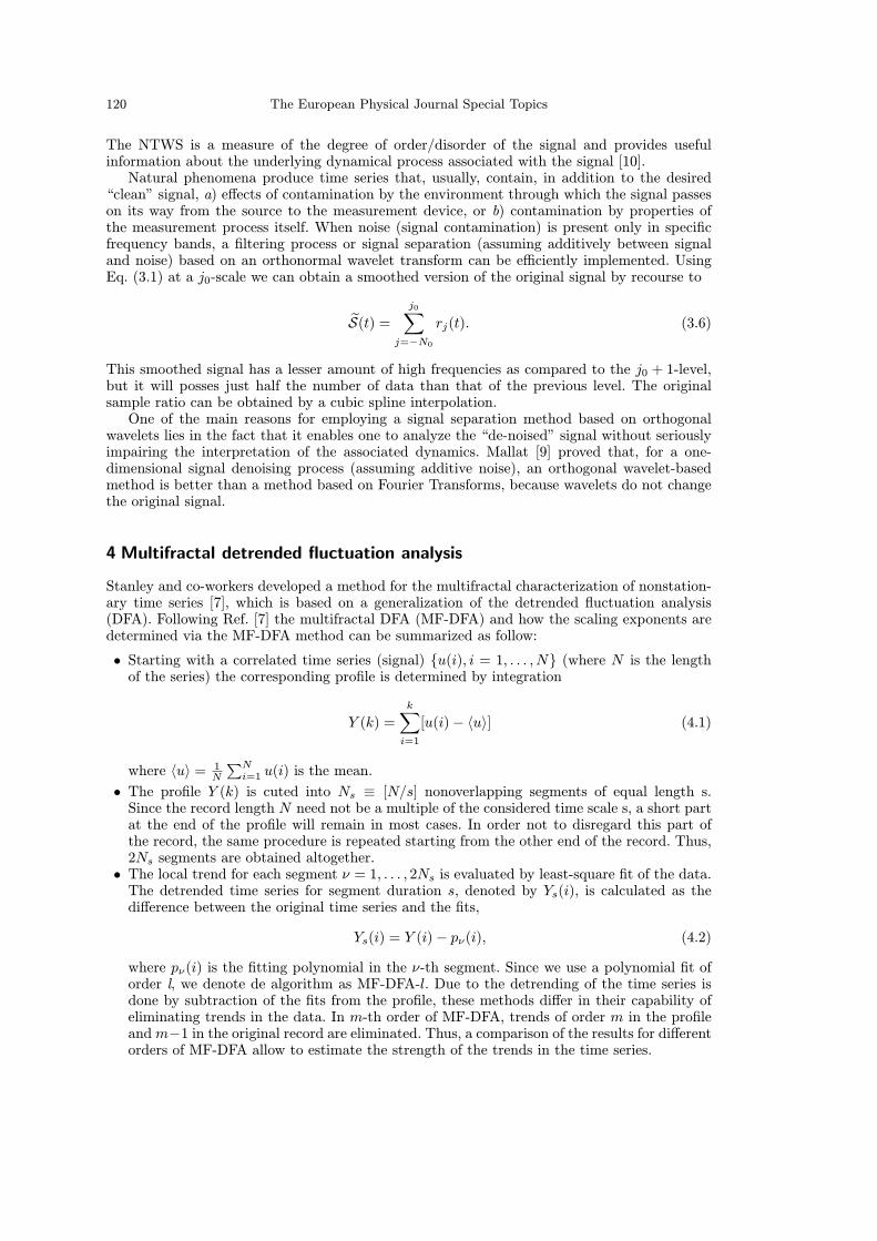
Three secondary generalized TCES from a female epileptic patient admitted for video-EEGmonitoring were here analyzed (patient B in Table 1 of Ref. [6]). The patient has diagnosisof pharmaco-resistant epilepsy and no other accompanying disorders. Scalp electrodes withbimastoideal reference were applied following the 10-20 international system. Each signal wasdigitized at 409.6Hz through a 12 bit A/D converter and filtered with an “antialiasing” 8 polelow pass Bessel filter, with a cutoff frequency of 50Hz. Then, the signal was digitally filteredwith a 1–50Hz bandpass filter (physician frequency range of interest for diagnosis) and stored,after decimation, at ωs = 102.4Hz (sample frequency) in a PC hard drive. Analysis for eachevent included 60 s of EEG before the seizure onset and 120 s of ictal and post-ictal phases. All180 s were analyzed at the right central region, C4 derivation. This electrode has been chosenafter visual inspection of the EEG, by the physician team, as the one with the least numberof artifacts. The time intervals of the pre-ictal stage which present artifacts (ocular and othermovements, etc.) were marked by the physician team and were excluded in the subsequentanalysis.As an example, in Fig. 1 we present a scalp EEG signal (first seizure) corresponding to a

TCES recorded over C4 channel. In this record, pre-ictal phase is characterized by amplitudesignal ∼ 50µV. The epileptic seizure starts at 80 s, with a “discharge” of slow waves superposedby fast ones with lower amplitude. This discharge lasts approximately 8 s and has a meanamplitude of 100µV. Afterwards, the seizure spreads, making the analysis of the EEG morecomplicated due to muscle artifacts; however, by the video EEG it is possible to establish thebeginning of the clonic phase at around 125 s, and the end of the seizure at 155 s, where thereis an abrupt decay of the signal’s amplitude.

3 Wavelet quantifiers and wavelet filtering

Wavelet analysis relies on the use of an appropriate basis and a characterization of the signalby the amplitude-distribution in such a basis [8,9]. The wavelet coefficients efficiently provideboth full information and a direct estimation of local energies at the different scales.Our EEG signal is assumed to be given by the sampled values S = {s0(k); k = 1, . . . ,M},

corresponding to a uniform time grid. If the discrete diadic wavelet decomposition is carriedout over all resolutions levels, j = −N0, . . . ,−1 (N0 = log2[M ], with M the number samples)the wavelet expansion reads

S(t) =−1∑

j=−N0

∑k

Cj(k) ψj,k(t) =

−1∑j=−N0

rj(t), (3.1)

where ψj,k(t) = 2j/2 ψ(2jt−k) with j, k ∈ Z and ψ(t) the mother wavelet. k is the time index

and at each wavelet resolution level j one have Nj = 2jM coefficients. The wavelet coefficients

Cj(k) can be interpreted as the local residual errors between successive signal approximations

Complex Systems – New Trends and Expectations 119

Fig. 1. Scalp EEG signal for a TCES, recordedat central right location (C4). The seizurestarts at 80 s and the clonic phase at 125 s. Theseizure ends at 155 s.

at scales j and j+1 [8,9]. The above expansion yields information on the signal S(t) pertainingto the frequencies 2j−1ωs ≤ |ω| ≤ 2jωs.If the family {ψj,k(t)} is an orthonormal basis for L2(R), the concept of energy is linked

with the usual notions derived from Fourier’s theory. The wavelet coefficients are given byCj(k) = 〈S, ψj,k〉 and the energy, at each resolution level j = −N0, . . . ,−1, will be the energyof the detail signal

Ej =∑k

|Cj(k)|2. (3.2)

The total energy can be obtained in the fashion

Etot =

−1∑j=−N0

∑k

|Cj(k)|2 =−1∑

j=−N0Ej . (3.3)

Finally, we define the normalized ρj-values, which represent the relative wavelet energy (RWE)

ρj = Ej/Etot (3.4)

for the resolution levels j = −N0, . . . ,−1. The RWE, ρj , yield at different scales the probabilitydistribution for the energy. Clearly,

∑−1j=−N0 ρj = 1 and the distribution {ρj ; j = −N0, . . . ,−1}

can be considered as a time-scale density that constitutes a suitable tool for detecting andcharacterizing specific phenomena in both the time and the frequency planes [4–6].Shannon’s information measure gives a criterion for analyzing and comparing probability

distributions. It measures the informative content of any distribution. We define the normalizedtotal wavelet entropy (NTWS) as

H = −−1∑

j=−N0ρj · ln [ρj ] / ln[N0]. (3.5)

120 The European Physical Journal Special Topics

The NTWS is a measure of the degree of order/disorder of the signal and provides usefulinformation about the underlying dynamical process associated with the signal [10].Natural phenomena produce time series that, usually, contain, in addition to the desired

“clean” signal, a) effects of contamination by the environment through which the signal passeson its way from the source to the measurement device, or b) contamination by properties ofthe measurement process itself. When noise (signal contamination) is present only in specificfrequency bands, a filtering process or signal separation (assuming additively between signaland noise) based on an orthonormal wavelet transform can be efficiently implemented. UsingEq. (3.1) at a j0-scale we can obtain a smoothed version of the original signal by recourse to

S(t) =j0∑

j=−N0rj(t). (3.6)

This smoothed signal has a lesser amount of high frequencies as compared to the j0 + 1-level,but it will posses just half the number of data than that of the previous level. The originalsample ratio can be obtained by a cubic spline interpolation.One of the main reasons for employing a signal separation method based on orthogonal

wavelets lies in the fact that it enables one to analyze the “de-noised” signal without seriouslyimpairing the interpretation of the associated dynamics. Mallat [9] proved that, for a one-dimensional signal denoising process (assuming additive noise), an orthogonal wavelet-basedmethod is better than a method based on Fourier Transforms, because wavelets do not changethe original signal.

4 Multifractal detrended fluctuation analysis

Stanley and co-workers developed a method for the multifractal characterization of nonstation-ary time series [7], which is based on a generalization of the detrended fluctuation analysis(DFA). Following Ref. [7] the multifractal DFA (MF-DFA) and how the scaling exponents aredetermined via the MF-DFA method can be summarized as follow:

• Starting with a correlated time series (signal) {u(i), i = 1, . . . , N} (where N is the lengthof the series) the corresponding profile is determined by integration

Y (k) =k∑i=1

[u(i)− 〈u〉] (4.1)

where 〈u〉 = 1N

∑Ni=1 u(i) is the mean.

• The profile Y (k) is cuted into Ns ≡ [N/s] nonoverlapping segments of equal length s.Since the record length N need not be a multiple of the considered time scale s, a short partat the end of the profile will remain in most cases. In order not to disregard this part ofthe record, the same procedure is repeated starting from the other end of the record. Thus,2Ns segments are obtained altogether.

• The local trend for each segment ν = 1, . . . , 2Ns is evaluated by least-square fit of the data.The detrended time series for segment duration s, denoted by Ys(i), is calculated as thedifference between the original time series and the fits,

Ys(i) = Y (i)− pν(i), (4.2)

where pν(i) is the fitting polynomial in the ν-th segment. Since we use a polynomial fit oforder l, we denote de algorithm as MF-DFA-l. Due to the detrending of the time series isdone by subtraction of the fits from the profile, these methods differ in their capability ofeliminating trends in the data. In m-th order of MF-DFA, trends of order m in the profileandm−1 in the original record are eliminated. Thus, a comparison of the results for differentorders of MF-DFA allow to estimate the strength of the trends in the time series.

Complex Systems – New Trends and Expectations 121

• For each of the 2Ns segments the variance of the detrended time series Ys(i) is evaluatedby averaging over all data point i in the ν-th segment

F 2s (ν) =1

s

s∑i=1

{Ys[(ν − 1)s+ i]}2. (4.3)

• Average over all segments to obtain the q-th fluctuation function

Fq(s) =

{1

2Ns

2Ns∑ν=1

[F 2s (ν)]q/2

}1/q, (4.4)

where, in general, the index q can take any real value. For q = 2, the standard DFA procedureis retrieved.

• The scaling behavior of the fluctuation is determined by analyzing log-log plots Fq(s) versuss for each value of q. If the series u(i) are long-range power-low correlated Fq(s) increase,for large values of s, as a power-law

Fq(s) ∼ sh(q) . (4.5)

For q = 0 the value h(0) cannot be determined directly using the average procedure inEq. (4.4) because of the diverging exponent. Instead, a logarithmic average procedure hasto be employed,

F0(s) = exp

{1

4Ns

2Ns∑ν=1

ln[F 2s (ν)

]} ∼ sh(0) . (4.6)

For monofractal time series with compact support, h(q) is independent of q, since the scalingbehavior of the variance F 2s (ν) is identical for all segments ν, and the averaging procedurein Eq. (4.4) will give just this identical scaling behavior for all values of q. Only if smalland large fluctuations scale differently, there will be a significant dependence of h(q) on q: Ifwe consider positive values of q, the segments ν with large variance F 2s (ν) will dominate theaverage Fq(s). Thus, for positive values of q, h(q) describes the scaling behavior of the segmentswith large fluctuations. On the contrary, for negative values of q, the segments ν with smallvariance F 2s (ν) will dominate the average Fq(s). Hence, for negative values of q, h(q) describethe scaling behavior of the segments with small fluctuations.Following Eqs. (4.4) and (4.6) and assume that the length N of the series is an integer

multiple of the scale s,N/s∑ν

| Y (νs)− Y ((ν − 1)s) |q∼ sqh(q)−1. (4.7)

Stanley and co-workers show that this multifractal formalism corresponding with the standardbox counting theory, and they related both formalisms. It is obvious that the term Y (νs) −Y ((ν−1)s) is identical to the sum of the numbers u(i) whitin each segment ν of size s. This sumis the box probability ps(ν) in the standard formalism for normalized series u(i). The scalingexponent τ(q) is usually defined via the partition function Zq(s),

Zq(s) ≡N/s∑ν=1

| ps(ν) |q∼ sτ(q) (4.8)

where q is a real parameter as in the MF-DFA. Then using the last equation and Eq. (4.8),they conclude that are identically and obtain the relation between the two sets of multifractalscaling exponents:

τ(q) = qh(q)− 1. (4.9)

The singularity spectrum f(α) is another way to characterize the multifractality of the series.The parameter α is the Holder exponent or the singularity intensity. The f(α) spectrum isrealted with τ(q) via a Legendre transformation: α = τ ′(q) and f(α) = qα − τ(q), and usingEq. (4.9) they related directely α and f(α) to h(q): α = h(q)+qh′(q) and f(α) = q[α−h(q)]+1.

122 The European Physical Journal Special Topics

Fig. 2. a) Spectrum of the MF-DFA1 fluctuation versus q range between –80 to 80 (step 1) for thetonic (110–124 s) and clonic (124–145 s) phases corresponding to the EEG-TCES shown in Fig. 1.b) τ(q) for the tonic and clonic phases.

5 Results and discussion

In the present study, an orthogonal decimated discrete wavelet transform (ODWT) wasapplied, in which orthogonal cubic spline function were used as mother wavelets, ψ, and thetime-frequency information was organized in a hierarchical scheme [8,9]. We define six fre-quency bands for an appropriate wavelet analysis within the multiresolution scheme to be used.We denoted these band-resolution levels by Bj (|j| = 1, . . . , 6). Their frequency limits, timeresolution, as well as their correspondence with traditional EEG frequency bands, are given inTable 2 of Ref. [6].Electrical muscular activity can be associated with frequencies (≥ 20Hz) in the range fre-

quency bands B1 and B2, at wavelet resolution levels j = −1 and −2, respectively [2]. Then thecontributions corresponding to B1 and B2, containing high frequency artifacts related to mus-cular activity that blurred the EEG, were not take into account for the evaluation of the waveletbased quantifiers (setting to zero their corresponding contributions). Although high frequencybrain activity is thereby also eliminated, its contributions during the ictal stage is not as strongas it is for middle and low frequencies [4]. In order to make a behavior “quantification”, thetemporal evolution of the above defined quantifiers (RWE and NTWS), the wavelet coefficientsseries {Cj(k)} of the analyzed signal are divided into non-overlapping temporal windows oflength L and, for each interval i (i = 1, . . . , NT , with NT =M/L), the different quantifiers areevaluated [4–6]. In the present study the time-window width employed was of L = 2.5 s each(M = 256 data).Noise-free EEG signal, without muscular activity contributions (frequency bands B1 and

B2) is reconstructed using wavelet resolution levels j = −3 to −6 (j0 and N0 values in Eq. (3.6)respectively), and its corresponding dynamics scaling behavior is performed. The time intervalassociated with the ERR was identified by the union of the two periods, in the ictal phase, forwhich the RWE plateau criteria (see discussion and implementation in Ref. [4]) for frequency

Complex Systems – New Trends and Expectations 123

Table 1. Characteristic slopes of τ(q) for the three different seizures corresponding to the same patient.

Tonic Phase Clonic PhaseSeizure q < 0 q > 0 q < 0 q > 0

B1 1.38 1.01 1.26 0.99B2 1.35 0.94 1.27 1.02B3 1.31 0.91 1.20 0.97

bands B5 and B6 (0.8–3.2Hz, delta activity) are satisfied. The time for the tonic to clonic phasetransition was identified as the corresponding time for which the NTWS present the absoluteminimum value in the ictal period [4,6]. In TCES display in Fig. 1, the ERR is identifiedbetween the 110 s and 145 s and, the transition from tonic to clonic phase at 124 s in agreementwith the observed in the video monitoring. Two time series are considered: the associated withthe tonic (110–124 s) and the clonic (124–145 s) phases. The corresponding results of MF-DFA1analysis for the EEG epileptic seizure display in Fig. 1 are shown in Fig. 2.Figure 2a shows the obtained q dependence of the asymptotic scaling exponent h(q) for

the tonic and clonic phases. These results suggest that do not exist (or it is very week) adependence with the parameter q. In consequence we can conclude that the ERR does notshow a multifractal behaviour. However, numerical differences are observed for the two phases(see Fig. 2(a)), in particular, for q < 0. We use this fact for characterization of the tonic andclonic phases.For q > 0 almost no differences between the two phases are observed for the scaling behaviour

of the segments with large fluctuations. Contrary, for q < 0, clear differentiation betweenthe tonic and clonic phases are present in the scaling behaviour of the segments with smallfluctuations. A quantification of this effect can be do it measuring the slope of the lineardependence of τ(q) with q (linear fit τ(q) = aq + b), obtaining slope values of a = 1.01 (q > 0)and a = 1.38 (q < 0) for tonic phase and, a = 0.99 (q > 0) and a = 1.26 (q < 0) for clonic phaserespectively (see Fig. 2(b)). In summary, one can associate a monofractal scaling behaviour tothe observed ERR, with small values for clonic phase. Note that, this behaviour is compatiblewith the observed decrease in time of the central frequency associate to the ERR induced bythe epileptic focus consider as a global pacemaker [11].Similar analysis was performed for the other two EEG-TCES. In Table 1, the obtained

slope values, for q < 0 and q > 0 for the three TCES analyzed are given. Note the similarityin the obtained values for the different seizures. This low variability implies that we can asso-ciate a monofractal scaling behaviour to the patient and in consequence could be used for acharacterization of the electrophysiology of the generalized TCES.

References

1. H. Gastaut, R. Broughton, Epileptic Seizures (Charles C. Thomas, Springfield, 1972)2. E. Niedermeyer, F.H. Lopes da Silva, Electroencephalography, Basic Principles, Clinical Appli-cations, and Related Field (Williams & Wilkins, Baltimore, 1999), p. 1135

3. T.M. Darcey, P.D. Willamson, Electroenceph. Clin. Neurophysiol. 61, 573 (1985)4. O.A. Rosso, S. Blanco, A. Rabinowicz, Signal Processing 86, 1275 (2003); and references therein5. O.A. Rosso, M.T. Martin, A. Plastino A, Physica A 347, 444 (2005)6. O.A. Rosso, M.T. Martin, A. Figliola, K. Keller, A. Plastino, J. Neurosci. Meth. 153, 163 (2006);and references therein

7. J.W. Kantelhardt, S.A. Zschiegner, E. Koscielny-Bunde, S. Havlin, A. Bunde, H.E. Stanley, PhysicaA 316, 87 (2002)

8. I. Daubechies, Ten Lectures on Wavelets (SIAM, Philadelphia, 1992)9. S. Mallat, A Wavelet Tour of Signal Processing (Academic Press, San Diego, 1999)10. O.A. Rosso, M.L. Mairal, Physica A 312, 469 (2002)11. S. Blanco, A. Figliola, R. Quian Quiroga, O.A. Rosso, E. Serrano, Phys. Rev. E 57, 932 (1998)