epipolar geometry and the fundamental matrixvgg/hzbook/hzbook1/hzepipolar.pdf · epipolar geometry...
TRANSCRIPT

8
Epipolar Geometry and the Fundamental Matrix
The epipolar geometry is the intrinsic projective geometry between two views. It isindependent of scene structure, and only depends on the cameras’ internal param-eters and relative pose.
The fundamental matrix F encapsulates this intrinsic geometry. It is a 3 × 3matrix of rank 2. If a point in 3-space X is imaged as x in the first view, and x′ inthe second, then the image points satisfy the relation x′>Fx = 0.
We will first describe epipolar geometry, and derive the fundamental matrix.The properties of the fundamental matrix are then elucidated, both for generalmotion of the camera between the views, and for several commonly occurring specialmotions. It is next shown that the cameras can be retrieved from F up to a projectivetransformation of 3-space. This result is the basis for the projective reconstructiontheorem given in chapter 9. Finally, if the camera internal calibration is known, it isshown that the Euclidean motion of the cameras between views may be computedfrom the fundamental matrix up to a finite number of ambiguities.
The fundamental matrix is independent of scene structure. However, it can becomputed from correspondences of imaged scene points alone, without requiringknowledge of the cameras’ internal parameters or relative pose. This computationis described in chapter 10.
8.1 Epipolar geometry
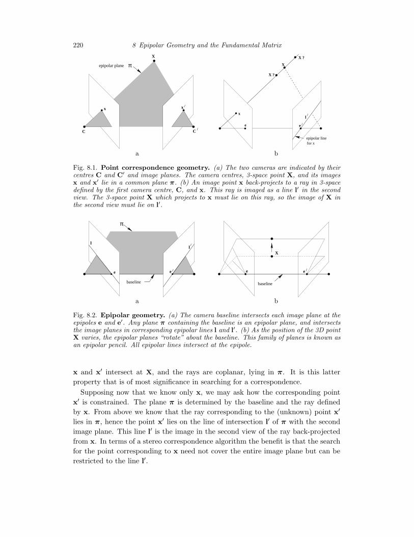
The epipolar geometry between two views is essentially the geometry of the inter-section of the image planes with the pencil of planes having the baseline as axis (thebaseline is the line joining the camera centres). This geometry is usually motivatedby considering the search for corresponding points in stereo matching, and we willstart from that objective here.
Suppose a point X in 3-space is imaged in two views, at x in the first, and x′
in the second. What is the relation between the corresponding image points x andx′? As shown in figure 8.1a the image points x and x′, space point X, and cameracentres are coplanar. Denote this plane as π. Clearly, the rays back-projected from
219
220 8 Epipolar Geometry and the Fundamental Matrix
C C /
π
x x
X
epipolar plane
/
x
e
X ?
X
X ?
l
e
epipolar linefor x
/
/
a b
Fig. 8.1. Point correspondence geometry. (a) The two cameras are indicated by theircentres C and C′ and image planes. The camera centres, 3-space point X, and its imagesx and x′ lie in a common plane π. (b) An image point x back-projects to a ray in 3-spacedefined by the first camera centre, C, and x. This ray is imaged as a line l′ in the secondview. The 3-space point X which projects to x must lie on this ray, so the image of X inthe second view must lie on l′.
l
e e
l
π
baseline
/
/
e e
baseline
/
X
a b
Fig. 8.2. Epipolar geometry. (a) The camera baseline intersects each image plane at theepipoles e and e′. Any plane π containing the baseline is an epipolar plane, and intersectsthe image planes in corresponding epipolar lines l and l′. (b) As the position of the 3D pointX varies, the epipolar planes “rotate” about the baseline. This family of planes is known asan epipolar pencil. All epipolar lines intersect at the epipole.
x and x′ intersect at X, and the rays are coplanar, lying in π. It is this latterproperty that is of most significance in searching for a correspondence.
Supposing now that we know only x, we may ask how the corresponding pointx′ is constrained. The plane π is determined by the baseline and the ray definedby x. From above we know that the ray corresponding to the (unknown) point x′
lies in π, hence the point x′ lies on the line of intersection l′ of π with the secondimage plane. This line l′ is the image in the second view of the ray back-projectedfrom x. In terms of a stereo correspondence algorithm the benefit is that the searchfor the point corresponding to x need not cover the entire image plane but can berestricted to the line l′.
8.1 Epipolar geometry 221
e /e
a
b c
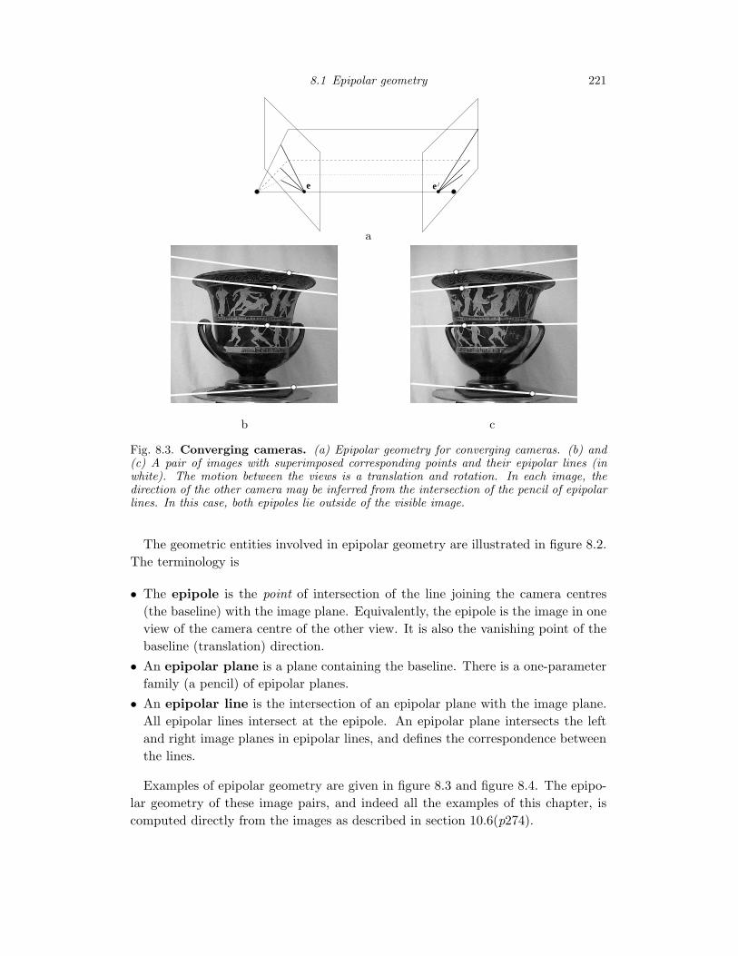
Fig. 8.3. Converging cameras. (a) Epipolar geometry for converging cameras. (b) and(c) A pair of images with superimposed corresponding points and their epipolar lines (inwhite). The motion between the views is a translation and rotation. In each image, thedirection of the other camera may be inferred from the intersection of the pencil of epipolarlines. In this case, both epipoles lie outside of the visible image.
The geometric entities involved in epipolar geometry are illustrated in figure 8.2.The terminology is
• The epipole is the point of intersection of the line joining the camera centres(the baseline) with the image plane. Equivalently, the epipole is the image in oneview of the camera centre of the other view. It is also the vanishing point of thebaseline (translation) direction.
• An epipolar plane is a plane containing the baseline. There is a one-parameterfamily (a pencil) of epipolar planes.
• An epipolar line is the intersection of an epipolar plane with the image plane.All epipolar lines intersect at the epipole. An epipolar plane intersects the leftand right image planes in epipolar lines, and defines the correspondence betweenthe lines.
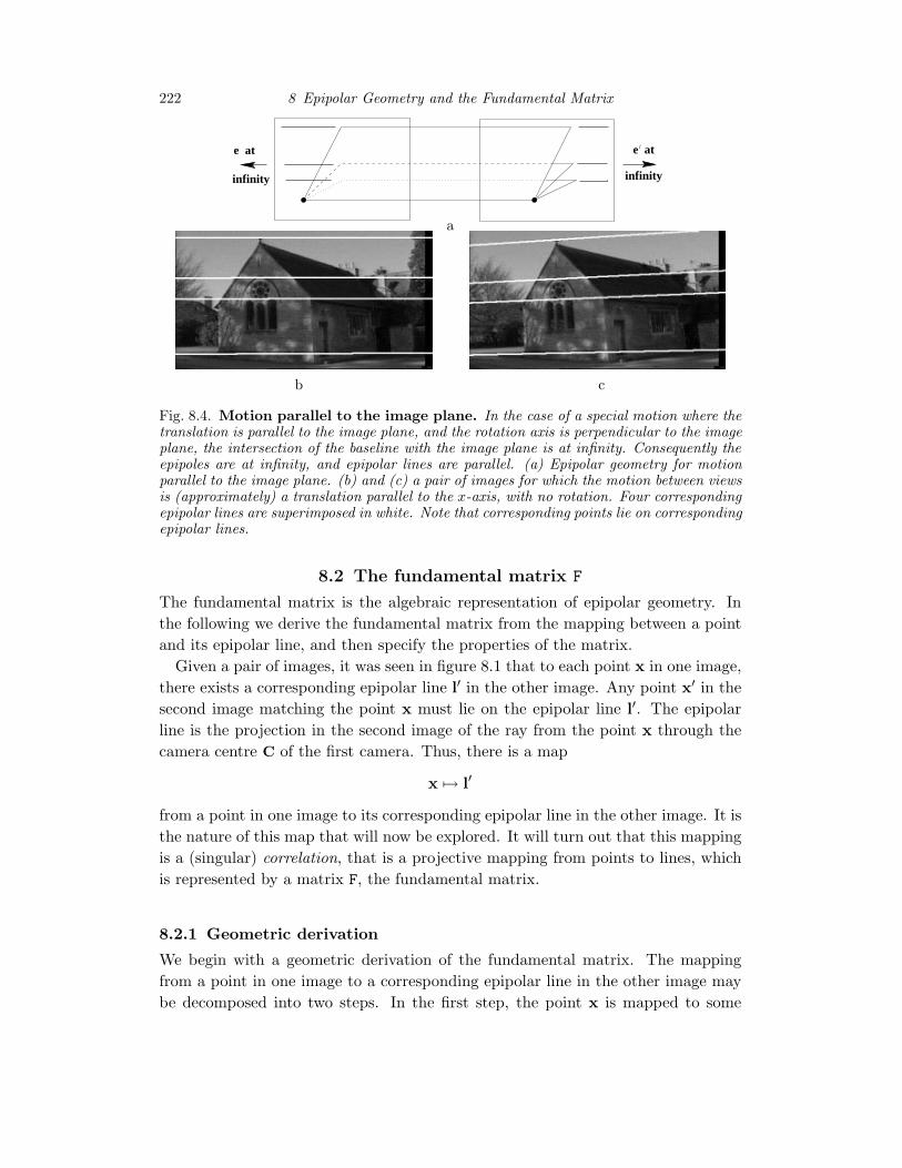
Examples of epipolar geometry are given in figure 8.3 and figure 8.4. The epipo-lar geometry of these image pairs, and indeed all the examples of this chapter, iscomputed directly from the images as described in section 10.6(p274).
222 8 Epipolar Geometry and the Fundamental Matrix
e at
infinity
e at/
infinity
a
b c
Fig. 8.4. Motion parallel to the image plane. In the case of a special motion where thetranslation is parallel to the image plane, and the rotation axis is perpendicular to the imageplane, the intersection of the baseline with the image plane is at infinity. Consequently theepipoles are at infinity, and epipolar lines are parallel. (a) Epipolar geometry for motionparallel to the image plane. (b) and (c) a pair of images for which the motion between viewsis (approximately) a translation parallel to the x-axis, with no rotation. Four correspondingepipolar lines are superimposed in white. Note that corresponding points lie on correspondingepipolar lines.
8.2 The fundamental matrix F
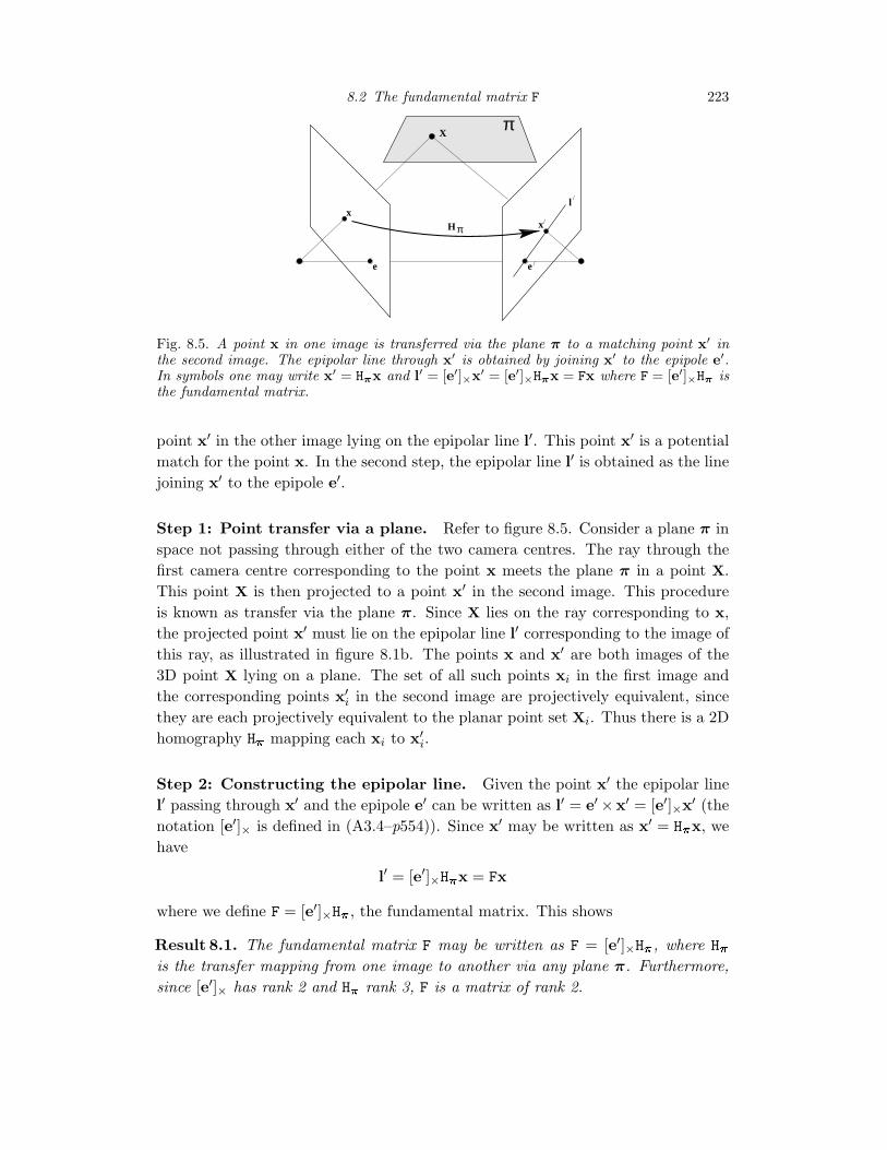
The fundamental matrix is the algebraic representation of epipolar geometry. Inthe following we derive the fundamental matrix from the mapping between a pointand its epipolar line, and then specify the properties of the matrix.
Given a pair of images, it was seen in figure 8.1 that to each point x in one image,there exists a corresponding epipolar line l′ in the other image. Any point x′ in thesecond image matching the point x must lie on the epipolar line l′. The epipolarline is the projection in the second image of the ray from the point x through thecamera centre C of the first camera. Thus, there is a map
x 7→ l′
from a point in one image to its corresponding epipolar line in the other image. It isthe nature of this map that will now be explored. It will turn out that this mappingis a (singular) correlation, that is a projective mapping from points to lines, whichis represented by a matrix F, the fundamental matrix.
8.2.1 Geometric derivation
We begin with a geometric derivation of the fundamental matrix. The mappingfrom a point in one image to a corresponding epipolar line in the other image maybe decomposed into two steps. In the first step, the point x is mapped to some
8.2 The fundamental matrix F 223
/e e
lx
/
H
X
/xπ
π
Fig. 8.5. A point x in one image is transferred via the plane π to a matching point x′ inthe second image. The epipolar line through x′ is obtained by joining x′ to the epipole e′.In symbols one may write x′ = Hπx and l′ = [e′]×x′ = [e′]×Hπx = Fx where F = [e′]×Hπ isthe fundamental matrix.
point x′ in the other image lying on the epipolar line l′. This point x′ is a potentialmatch for the point x. In the second step, the epipolar line l′ is obtained as the linejoining x′ to the epipole e′.
Step 1: Point transfer via a plane. Refer to figure 8.5. Consider a plane π inspace not passing through either of the two camera centres. The ray through thefirst camera centre corresponding to the point x meets the plane π in a point X.This point X is then projected to a point x′ in the second image. This procedureis known as transfer via the plane π. Since X lies on the ray corresponding to x,the projected point x′ must lie on the epipolar line l′ corresponding to the image ofthis ray, as illustrated in figure 8.1b. The points x and x′ are both images of the3D point X lying on a plane. The set of all such points xi in the first image andthe corresponding points x′i in the second image are projectively equivalent, sincethey are each projectively equivalent to the planar point set Xi. Thus there is a 2Dhomography H� mapping each xi to x′i.
Step 2: Constructing the epipolar line. Given the point x′ the epipolar linel′ passing through x′ and the epipole e′ can be written as l′ = e′×x′ = [e′]×x′ (thenotation [e′]× is defined in (A3.4–p554)). Since x′ may be written as x′ = H�x, wehave
l′ = [e′]×H�x = Fx
where we define F = [e′]×H�, the fundamental matrix. This shows
Result 8.1. The fundamental matrix F may be written as F = [e′]×H�, where H�is the transfer mapping from one image to another via any plane π. Furthermore,since [e′]× has rank 2 and H� rank 3, F is a matrix of rank 2.
224 8 Epipolar Geometry and the Fundamental Matrix
Geometrically, F represents a mapping from the 2-dimensional projective planeIP2 of the first image to the pencil of epipolar lines through the epipole e′. Thus, itrepresents a mapping from a 2-dimensional onto a 1-dimensional projective space,and hence must have rank 2.
Note, the geometric derivation above involves a scene plane π, but a plane is notrequired in order for F to exist. The plane is simply used here as a means of defininga point map from one image to another. The connection between the fundamentalmatrix and transfer of points from one image to another via a plane is dealt within some depth in chapter 12.
8.2.2 Algebraic derivation
The form of the fundamental matrix in terms of the two camera projection matrices,P, P′, may be derived algebraically. The following formulation is due to Xu andZhang [Xu-96].
The ray back-projected from x by P is obtained by solving PX = x. The one-parameter family of solutions is of the form given by (5.13–p148) as
X(λ) = P+x + λC
where P+ is the pseudo-inverse of P, i.e. PP+ = I, and C its null-vector, namely thecamera centre, defined by PC = 0. The ray is parametrized by the scalar λ. Inparticular two points on the ray are P+x (at λ = 0), and the first camera centre C(at λ = ∞). These two points are imaged by the second camera P′ at P′P+x andP′C respectively in the second view. The epipolar line is the line joining these twoprojected points, namely l′ = (P′C)× (P′P+x). The point P′C is the epipole in thesecond image, namely the projection of the first camera centre, and may be denotedby e′. Thus, l′ = [e′]×(P′P+)x = Fx, where F is the matrix
F = [e′]×P′P+. (8.1)
This is essentially the same formula for the fundamental matrix as the one derivedin the previous section, the homography H� having the explicit form H� = P′P+ interms of the two camera matrices. Note that this derivation breaks down in thecase where the two camera centres are the same for, in this case, C is the commoncamera centre of both P and P′, and so P′C = 0. It follows that F defined in (8.1) isthe zero matrix.
Example 8.2. Suppose the camera matrices are those of a calibrated stereo rig withthe world origin at the first camera
P = K[I | 0] P′ = K′[R | t].Then
P+ =
[K−1
0>
]C =
(01
)
8.2 The fundamental matrix F 225
and
F = [P′C]×P′P+
= [K′t]×K′RK−1 = K′−>[t]×RK−1 = K′−>R[R>t]×K−1 = K′−>RK>[KR>t]×(8.2)
where the various forms follow from result A3.3(p555). Note that the epipoles(defined as the image of the other camera centre) are
e = P
(−R>t
1
)= KR>t e′ = P′
(01
)= K′t. (8.3)
Thus we may write (8.2) as
F = [e′]×K′RK−1 = K′−>[t]×RK−1 = K′−>R[R>t]×K−1 = K′−>RK>[e]×. (8.4)
4The expression for the fundamental matrix can be derived in many ways, and indeedwill be derived again several times in this book. In particular, (16.3–p400) expressesF in terms of 4 × 4 determinants composed from rows of the camera matrices foreach view.
8.2.3 Correspondence condition
Up to this point we have considered the map x → l′ defined by F. We may nowstate the most basic properties of the fundamental matrix.
Result 8.3. The fundamental matrix satisfies the condition that for any pair ofcorresponding points x↔ x′ in the two images
x′>Fx = 0.
This is true, because if points x and x′ correspond, then x′ lies on the epipolarline l′ = Fx corresponding to the point x. In other words 0 = x′>l′ = x′>Fx.Conversely, if image points satisfy the relation x′>Fx = 0 then the rays defined bythese points are coplanar. This is a necessary condition for points to correspond.
The importance of the relation of result 8.3 is that it gives a way of characteriz-ing the fundamental matrix without reference to the camera matrices, i.e. only interms of corresponding image points. This enables F to be computed from imagecorrespondences alone. We have seen from (8.1) that F may be computed from thetwo camera matrices, P, P′, and in particular that F is determined uniquely fromthe cameras, up to an overall scaling. However, we may now enquire how manycorrespondences are required to compute F from x′>Fx = 0, and the circumstancesunder which the matrix is uniquely defined by these correspondences. The detailsof this are postponed until chapter 10, where it will be seen that in general at least7 correspondences are required to compute F.
226 8 Epipolar Geometry and the Fundamental Matrix
• F is a rank 2 homogeneous matrix with 7 degrees of freedom.
• Point correspondence: If x and x′ are corresponding image points, then
x′>Fx = 0.
• Epipolar lines:
� l′ = Fx is the epipolar line corresponding to x.
� l = F>x′ is the epipolar line corresponding to x′.
• Epipoles:
� Fe = 0.
� F>e′ = 0.
• Computation from camera matrices P, P′:� General cameras,
F = [e′]×P′P+, where P+ is the pseudo-inverse of P, and e′ = P′C, with PC = 0.
� Canonical cameras, P = [I | 0], P′ = [M |m],F = [e′]×M = M−>[e]×, where e′ = m and e = M−1m.
� Cameras not at infinity P = K[I | 0], P′ = K′[R | t],F = K′−>[t]×RK−1 = [K′t]×K′RK−1 = K′−>RK>[KR>t]×.
Table 8.1. Summary of fundamental matrix properties.
8.2.4 Properties of the fundamental matrix
Definition 8.4. Suppose we have two images acquired by cameras with non-coincident centres, then the fundamental matrix F is the unique 3 × 3 rank 2homogeneous matrix which satisfies
x′>Fx = 0 (8.5)
for all corresponding points x↔ x′.
We now briefly list a number of properties of the fundamental matrix. The mostimportant properties are also summarized in table 8.1.
(i) Transpose: If F is the fundamental matrix of the pair of cameras (P, P′),then F> is the fundamental matrix of the pair in the opposite order: (P′, P).
(ii) Epipolar lines: For any point x in the first image, the corresponding epipo-lar line is l′ = Fx. Similarly, l = F>x′ represents the epipolar line correspond-ing to x′ in the second image.
(iii) The epipole: for any point x (other than e) the epipolar line l′ = Fx containsthe epipole e′. Thus e′ satisfies e′>(Fx) = (e′>F)x = 0 for all x. It followsthat e′>F = 0, i.e. e′ is the left null-space of F. Similarly Fe = 0, i.e. e is theright null-space of F.
8.2 The fundamental matrix F 227
e e /
l3
l/2l
1
l
1l
3l/
/
2
p
a b
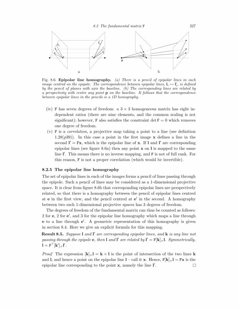
Fig. 8.6. Epipolar line homography. (a) There is a pencil of epipolar lines in eachimage centred on the epipole. The correspondence between epipolar lines, li ↔ l′i, is definedby the pencil of planes with axis the baseline. (b) The corresponding lines are related bya perspectivity with centre any point p on the baseline. It follows that the correspondencebetween epipolar lines in the pencils is a 1D homography.
(iv) F has seven degrees of freedom: a 3 × 3 homogeneous matrix has eight in-dependent ratios (there are nine elements, and the common scaling is notsignificant); however, F also satisfies the constraint det F = 0 which removesone degree of freedom.
(v) F is a correlation, a projective map taking a point to a line (see definition1.28(p39)). In this case a point in the first image x defines a line in thesecond l′ = Fx, which is the epipolar line of x. If l and l′ are correspondingepipolar lines (see figure 8.6a) then any point x on l is mapped to the sameline l′. This means there is no inverse mapping, and F is not of full rank. Forthis reason, F is not a proper correlation (which would be invertible).
8.2.5 The epipolar line homography
The set of epipolar lines in each of the images forms a pencil of lines passing throughthe epipole. Such a pencil of lines may be considered as a 1-dimensional projectivespace. It is clear from figure 8.6b that corresponding epipolar lines are perspectivelyrelated, so that there is a homography between the pencil of epipolar lines centredat e in the first view, and the pencil centred at e′ in the second. A homographybetween two such 1-dimensional projective spaces has 3 degrees of freedom.
The degrees of freedom of the fundamental matrix can thus be counted as follows:2 for e, 2 for e′, and 3 for the epipolar line homography which maps a line throughe to a line through e′. A geometric representation of this homography is givenin section 8.4. Here we give an explicit formula for this mapping.
Result 8.5. Suppose l and l′ are corresponding epipolar lines, and k is any line notpassing through the epipole e, then l and l′ are related by l′ = F[k]×l. Symmetrically,l = F>[k′]×l′.
Proof The expression [k]×l = k × l is the point of intersection of the two lines kand l, and hence a point on the epipolar line l – call it x. Hence, F[k]×l = Fx is theepipolar line corresponding to the point x, namely the line l′.
228 8 Epipolar Geometry and the Fundamental Matrix
cameracentre
parallellines
pointvanishing
image
e
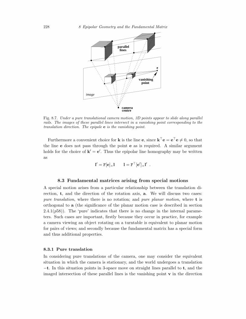
Fig. 8.7. Under a pure translational camera motion, 3D points appear to slide along parallelrails. The images of these parallel lines intersect in a vanishing point corresponding to thetranslation direction. The epipole e is the vanishing point.
Furthermore a convenient choice for k is the line e, since k>e = e>e 6= 0, so thatthe line e does not pass through the point e as is required. A similar argumentholds for the choice of k′ = e′. Thus the epipolar line homography may be writtenas
l′ = F[e]×l l = F>[e′]×l′ .
8.3 Fundamental matrices arising from special motions
A special motion arises from a particular relationship between the translation di-rection, t, and the direction of the rotation axis, a. We will discuss two cases:pure translation, where there is no rotation; and pure planar motion, where t isorthogonal to a (the significance of the planar motion case is described in section2.4.1(p58)). The ‘pure’ indicates that there is no change in the internal parame-ters. Such cases are important, firstly because they occur in practice, for examplea camera viewing an object rotating on a turntable is equivalent to planar motionfor pairs of views; and secondly because the fundamental matrix has a special formand thus additional properties.
8.3.1 Pure translation
In considering pure translations of the camera, one may consider the equivalentsituation in which the camera is stationary, and the world undergoes a translation−t. In this situation points in 3-space move on straight lines parallel to t, and theimaged intersection of these parallel lines is the vanishing point v in the direction

8.3 Fundamental matrices arising from special motions 229
ee //C C
a
b c
Fig. 8.8. Pure translational motion. (a) under the motion the epipole is a fixed point,i.e. has the same coordinates in both images, and points appear to move along lines radiatingfrom the epipole. The epipole in this case is termed the Focus of Expansion (FOE). (b) and(c) the same epipolar lines are overlaid in both cases. Note the motion of the posters on thewall which slide along the epipolar line.
of t. This is illustrated in figure 8.7 and figure 8.8. It is evident that v is the epipolefor both views, and the imaged parallel lines are the epipolar lines. The algebraicdetails are given in the following example.
Example 8.6. Suppose the motion of the cameras is a pure translation with norotation and no change in the internal parameters. One may assume that the twocameras are P = K[I | 0] and P′ = K[I | t]. Then from (8.4) (using R = I and K = K′)
F = [e′]×KK−1 = [e′]×.
If the camera translation is parallel to the x-axis, then e′ = (1, 0, 0)>, so
F =
0 0 00 0 −10 1 0
.
The relation between corresponding points, x′>Fx = 0, reduces to y = y′, i.e. theepipolar lines are corresponding rasters. This is the situation that is sought byimage rectification described in section 10.12(p289). 4
Indeed if the image point x is normalized as x = (x, y, 1)>, then fromx = PX = K[I | 0]X, the space point’s (inhomogeneous) coordinates are (x,y, z)> =

230 8 Epipolar Geometry and the Fundamental Matrix
zK−1x, where z is the depth of the point X (the distance of X from the cameracentre measured along the principal axis of the first camera). It then follows fromx′ = P′X = K[I | t]X that the mapping from an image point x to an image point x′
is
x′ = x + Kt/z. (8.6)
The motion x′ = x+Kt/z of (8.6) shows that the image point “starts” at x and thenmoves along the line defined by x and the epipole e = e′ = v. The extent of themotion depends on the magnitude of the translation t (which is not a homogeneousvector here) and the inverse depth z, so that points closer to the camera appear tomove faster than those further away – a common experience when looking out of atrain window.
Note that in this case of pure translation F = [e′]× is skew-symmetric and hasonly 2 degrees of freedom, which correspond to the position of the epipole. Theepipolar line of x is l′ = Fx = [e]×x, and x lies on this line since x>[e]×x = 0, i.e.x, x′ and e = e′ are collinear (assuming both images are overlaid on top of eachother). This collinearity property is termed auto-epipolar, and does not hold forgeneral motion.
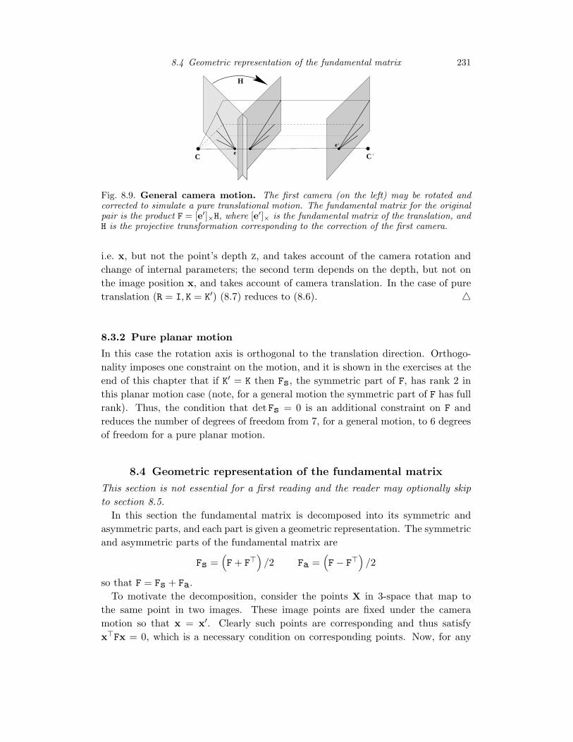
General motion. The pure translation case gives additional insight into thegeneral motion case. Given two arbitrary cameras, we may rotate the camera usedfor the first image so that it is aligned with the second camera. This rotation maybe simulated by applying a projective transformation to the first image. A furthercorrection may be applied to the first image to account for any difference in thecalibration matrices of the two images. The result of these two corrections is aprojective transformation H of the first image. If one assumes these corrections tohave been made, then the effective relationship of the two cameras to each other isthat of a pure translation. Consequently, the fundamental matrix corresponding tothe corrected first image and the second image is of the form F = [e′]×, satisfyingx′>Fx = 0, where x = Hx is the corrected point in the first image. From this onededuces that x′>[e′]×Hx = 0, and so the fundamental matrix corresponding to theinitial point correspondences x↔ x′ is F = [e′]×H. This is illustrated in figure 8.9.
Example 8.7. Continuing from example 8.2, assume again that the two camerasare P = K[I | 0] and P′ = K′[R | t]. Then as described in section 7.4.2(p194) therequisite projective transformation is H = K′RK−1 = H∞, where H∞ is the infinitehomography (see section 12.4(p327)), and F = [e′]×H∞.
If the image point x is normalized as x = (x, y, 1)>, as in example 8.6, then(x,y, z)> = zK−1x, and from x = P′X = K′[R | t]X the mapping from an imagepoint x to an image point x′ is
x′ = K′RK−1x + K′t/z. (8.7)
The mapping is in two parts: the first term depends on the image position alone,
8.4 Geometric representation of the fundamental matrix 231
/e
/e
H
C C
Fig. 8.9. General camera motion. The first camera (on the left) may be rotated andcorrected to simulate a pure translational motion. The fundamental matrix for the originalpair is the product F = [e′]×H, where [e′]× is the fundamental matrix of the translation, andH is the projective transformation corresponding to the correction of the first camera.
i.e. x, but not the point’s depth z, and takes account of the camera rotation andchange of internal parameters; the second term depends on the depth, but not onthe image position x, and takes account of camera translation. In the case of puretranslation (R = I, K = K′) (8.7) reduces to (8.6). 4
8.3.2 Pure planar motion
In this case the rotation axis is orthogonal to the translation direction. Orthogo-nality imposes one constraint on the motion, and it is shown in the exercises at theend of this chapter that if K′ = K then Fs, the symmetric part of F, has rank 2 inthis planar motion case (note, for a general motion the symmetric part of F has fullrank). Thus, the condition that det Fs = 0 is an additional constraint on F andreduces the number of degrees of freedom from 7, for a general motion, to 6 degreesof freedom for a pure planar motion.
8.4 Geometric representation of the fundamental matrix
This section is not essential for a first reading and the reader may optionally skipto section 8.5.
In this section the fundamental matrix is decomposed into its symmetric andasymmetric parts, and each part is given a geometric representation. The symmetricand asymmetric parts of the fundamental matrix are
Fs =(F + F>
)/2 Fa =
(F− F>
)/2
so that F = Fs + Fa.To motivate the decomposition, consider the points X in 3-space that map to
the same point in two images. These image points are fixed under the cameramotion so that x = x′. Clearly such points are corresponding and thus satisfyx>Fx = 0, which is a necessary condition on corresponding points. Now, for any
232 8 Epipolar Geometry and the Fundamental Matrix
skew-symmetric matrix A the form x>Ax is identically zero. Consequently only thesymmetric part of F contributes to x>Fx = 0, which then reduces to x>Fsx = 0. Aswill be seen below the matrix Fs may be thought of as a conic in the image plane.
Geometrically the conic arises as follows. The locus of all points in 3-space forwhich x = x′ is known as the horopter curve. Generally this is a twisted cu-bic curve in 3-space (see section 2.3(p57)) passing through the two camera cen-tres [Maybank-93]. The image of the horopter is the conic defined by Fs. Wereturn to the horopter in chapter 21.
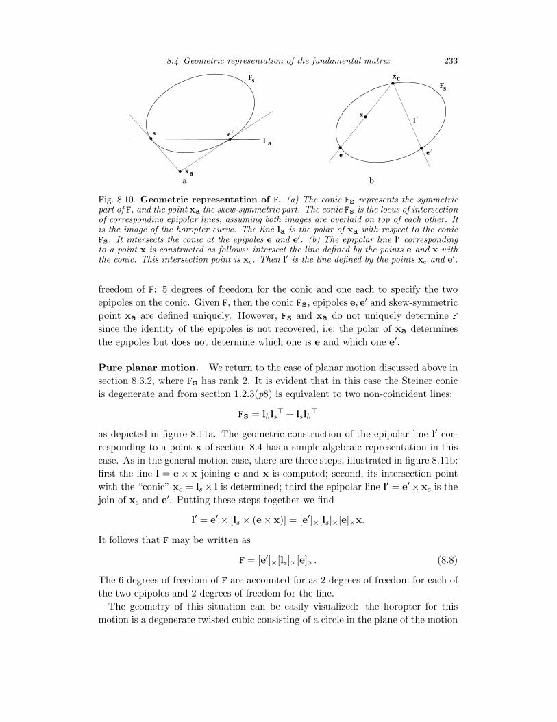
Symmetric part. The matrix Fs is symmetric and is of rank 3 in general. Ithas 5 degrees of freedom and is identified with a point conic, called the Steinerconic (the name is explained below). The epipoles e and e′ lie on the conic Fs.To see that the epipoles lie on the conic, i.e. that e>Fse = 0, start from Fe = 0.Then e>Fe = 0 and so e>Fse + e>Fae = 0. However, e>Fae = 0, since for anyanti-symmetric matrix S, x>Sx = 0. Thus e>Fse = 0. The derivation for e′ followsin a similar manner.
Anti-symmetric part. The matrix Fa is skew-symmetric and may be writtenas Fa = [xa]×, where xa is the null-vector of Fa. The skew-symmetric part has 2degrees of freedom and is identified with the point xa.
The relation between the point xa and conic Fs is shown in figure 8.10a. Thepolar of xa intersects the Steiner conic Fs at the epipoles e and e′ (the pole–polarrelation is described in section 1.2.3(p8)). The proof of this result is left as anexercise.
Epipolar line correspondence. It is a classical theorem of projective geometrydue to Steiner [Semple-79] that for two line pencils related by a homography, thelocus of intersections of corresponding lines is a conic. This is precisely the situationhere. The pencils are the epipolar pencils, one through e and the other through e′.The epipolar lines are related by a 1D homography as described in section 8.2.5.The locus of intersection is the conic Fs.
The conic and epipoles enable epipolar lines to be determined by a geometricconstruction as illustrated in figure 8.10b. This construction is based on the fixedpoint property of the Steiner conic Fs. The epipolar line l = x× e in the first viewdefines an epipolar plane in 3-space which intersects the horopter in a point, whichwe will call Xc. The point Xc is imaged in the first view at xc, which is the pointat which l intersects the conic Fs (since Fs is the image of the horopter). Now theimage of Xc is also xc in the second view due to the fixed-point property of thehoropter. So xc is the image in the second view of a point on the epipolar plane ofx. It follows that xc lies on the epipolar line l′ of x, and consequently l′ may becomputed as l′ = xc × e′.
The conic together with two points on the conic account for the 7 degrees of
8.4 Geometric representation of the fundamental matrix 233
e
F
a
/el
s
x a
Fs
e e
xl
xc
/
/
a b
Fig. 8.10. Geometric representation of F. (a) The conic Fs represents the symmetricpart of F, and the point xa the skew-symmetric part. The conic Fs is the locus of intersectionof corresponding epipolar lines, assuming both images are overlaid on top of each other. Itis the image of the horopter curve. The line la is the polar of xa with respect to the conicFs. It intersects the conic at the epipoles e and e′. (b) The epipolar line l′ correspondingto a point x is constructed as follows: intersect the line defined by the points e and x withthe conic. This intersection point is xc. Then l′ is the line defined by the points xc and e′.
freedom of F: 5 degrees of freedom for the conic and one each to specify the twoepipoles on the conic. Given F, then the conic Fs, epipoles e, e′ and skew-symmetricpoint xa are defined uniquely. However, Fs and xa do not uniquely determine F
since the identity of the epipoles is not recovered, i.e. the polar of xa determinesthe epipoles but does not determine which one is e and which one e′.
Pure planar motion. We return to the case of planar motion discussed above insection 8.3.2, where Fs has rank 2. It is evident that in this case the Steiner conicis degenerate and from section 1.2.3(p8) is equivalent to two non-coincident lines:
Fs = lhls> + lslh>
as depicted in figure 8.11a. The geometric construction of the epipolar line l′ cor-responding to a point x of section 8.4 has a simple algebraic representation in thiscase. As in the general motion case, there are three steps, illustrated in figure 8.11b:first the line l = e × x joining e and x is computed; second, its intersection pointwith the “conic” xc = ls× l is determined; third the epipolar line l′ = e′×xc is thejoin of xc and e′. Putting these steps together we find
l′ = e′ × [ls × (e× x)] = [e′]×[ls]×[e]×x.
It follows that F may be written as
F = [e′]×[ls]×[e]×. (8.8)
The 6 degrees of freedom of F are accounted for as 2 degrees of freedom for each ofthe two epipoles and 2 degrees of freedom for the line.
The geometry of this situation can be easily visualized: the horopter for thismotion is a degenerate twisted cubic consisting of a circle in the plane of the motion
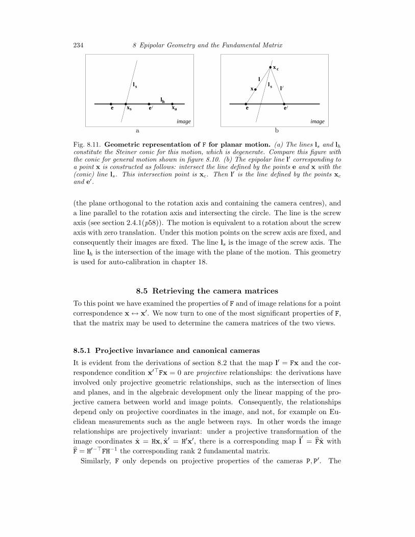
234 8 Epipolar Geometry and the Fundamental Matrix
e x el
xh
as /
l s
image
e e/
x c
l s l /
image
l
x
a b
Fig. 8.11. Geometric representation of F for planar motion. (a) The lines ls and lhconstitute the Steiner conic for this motion, which is degenerate. Compare this figure withthe conic for general motion shown in figure 8.10. (b) The epipolar line l′ corresponding toa point x is constructed as follows: intersect the line defined by the points e and x with the(conic) line ls. This intersection point is xc. Then l′ is the line defined by the points xc
and e′.
(the plane orthogonal to the rotation axis and containing the camera centres), anda line parallel to the rotation axis and intersecting the circle. The line is the screwaxis (see section 2.4.1(p58)). The motion is equivalent to a rotation about the screwaxis with zero translation. Under this motion points on the screw axis are fixed, andconsequently their images are fixed. The line ls is the image of the screw axis. Theline lh is the intersection of the image with the plane of the motion. This geometryis used for auto-calibration in chapter 18.
8.5 Retrieving the camera matrices
To this point we have examined the properties of F and of image relations for a pointcorrespondence x↔ x′. We now turn to one of the most significant properties of F,that the matrix may be used to determine the camera matrices of the two views.
8.5.1 Projective invariance and canonical cameras
It is evident from the derivations of section 8.2 that the map l′ = Fx and the cor-respondence condition x′>Fx = 0 are projective relationships: the derivations haveinvolved only projective geometric relationships, such as the intersection of linesand planes, and in the algebraic development only the linear mapping of the pro-jective camera between world and image points. Consequently, the relationshipsdepend only on projective coordinates in the image, and not, for example on Eu-clidean measurements such as the angle between rays. In other words the imagerelationships are projectively invariant: under a projective transformation of theimage coordinates x = Hx, x′ = H′x′, there is a corresponding map l
′= Fx with
F = H′−>FH−1 the corresponding rank 2 fundamental matrix.Similarly, F only depends on projective properties of the cameras P, P′. The
8.5 Retrieving the camera matrices 235
camera matrix relates 3-space measurements to image measurements and so dependson both the image coordinate frame and the choice of world coordinate frame. F
does not depend on the choice of world frame, for example a rotation of worldcoordinates changes P, P′, but not F. In fact, the fundamental matrix is unchangedby a projective transformation of 3-space. More precisely,
Result 8.8. If H is a 4 × 4 matrix representing a projective transformation of 3-space, then the fundamental matrices corresponding to the pairs of camera matrices(P, P′) and (PH, P′H) are the same.
Proof Observe that PX = (PH)(H−1X), and similarly for P′. Thus if x ↔ x′ arematched points with respect to the pair of cameras (P, P′), corresponding to a 3Dpoint X, then they are also matched points with respect to the pair of cameras(PH, P′H), corresponding to the point H−1X.
Thus, although from (8.1–p224) a pair of camera matrices (P, P′) uniquely deter-mine a fundamental matrix F, the converse is not true. The fundamental matrixdetermines the pair of camera matrices at best up to right-multiplication by a 3Dprojective transformation. It will be seen below that this is the full extent of theambiguity, and indeed the camera matrices are determined up to a projective trans-formation by the fundamental matrix.
Canonical form of camera matrices. Given this ambiguity, it is common todefine a specific canonical form for the pair of camera matrices corresponding toa given fundamental matrix in which the first matrix is of the simple form [I | 0],where I is the 3×3 identity matrix and 0 a null 3-vector. To see that this is alwayspossible, let P be augmented by one row to make a 4 × 4 non-singular matrix,denoted P∗. Now letting H = P∗−1, one verifies that PH = [I | 0] as desired.
The following result is very frequently used
Result 8.9. The fundamental matrix corresponding to a pair of camera matricesP = [I | 0] and P′ = [M |m] is equal to [m]×M.
This is easily derived as a special case of (8.1–p224).
8.5.2 Projective ambiguity of cameras given F
It has been seen that a pair of camera matrices determines a unique fundamentalmatrix. This mapping is not injective (one-to-one) however, since pairs of cameramatrices that differ by a projective transformation give rise to the same fundamen-tal matrix. It will now be shown that this is the only ambiguity. We will show thata given fundamental matrix determines the pair of camera matrices up to right mul-tiplication by a projective transformation. Thus, the fundamental matrix capturesthe projective relationship of the two cameras.
236 8 Epipolar Geometry and the Fundamental Matrix
Theorem8.10. Let F be a fundamental matrix and let (P, P′) and (P, P′) be two pairsof camera matrices such that F is the fundamental matrix corresponding to each ofthese pairs. Then there exists a non-singular 4 × 4 matrix H such that P = PH andP′ = P′H.
Proof Suppose that a given fundamental matrix F corresponds to two different pairsof camera matrices (P, P′) and (P, P′). As a first step, we may simplify the problemby assuming that each of the two pair of camera matrices is in canonical form withP = P = [I | 0], since this may be done by applying projective transformations toeach pair as necessary. Thus, suppose that P = P = [I | 0] and that P′ = [A | a] andP′ = [A | a]. According to result 8.9 the fundamental matrix may then be writtenF = [a]×A = [a]×A.We will need the following lemma:
Lemma 8.11. Suppose the rank 2 matrix F can be decomposed in two different waysas F = [a]×A and F = [a]×A; then a = ka and A = k−1(A + av>) for some non-zeroconstant k and 3-vector v.
Proof First, note that a>F = a>[a]×A = 0, and similarly, a>F = 0. Since F hasrank 2, it follows that a = ka as required. Next, from [a]×A = [a]×A it follows that[a]×
(kA− A
)= 0, and so kA − A = av> for some v. Hence, A = k−1(A + av>) as
required.
Applying this result to the two camera matrices P′ and P′ shows that P′ = [A | a]
and P′ = [k−1(A + av>) | ka] if they are to generate the same F. It only remains
now to show that these camera pairs are projectively related. Let H be the matrix
H =
[k−1I 0
k−1v> k
]. Then one verifies that PH = k−1[I | 0] = k−1P, and furthermore,
P′H = [A | a]H = [k−1(A + av>) | ka] = [A | a] = P′
so that the pairs P, P′ and P, P′ are indeed projectively related.
This can be tied precisely to a counting argument: the two cameras P and P′ eachhave 11 degrees of freedom, making a total of 22 degrees of freedom. To specify aprojective world frame requires 15 degrees of freedom (section 2.1(p45)), so once thedegrees of freedom of the world frame are removed from the two cameras 22−15 = 7degrees of freedom remain – which corresponds to the 7 degrees of freedom of thefundamental matrix.
8.5.3 Canonical cameras given F
We have shown that F determines the camera pair up to a projective transformationof 3-space. We will now derive a specific formula for a pair of cameras with canonical
8.5 Retrieving the camera matrices 237
form given F. We will make use of the following characterization of the fundamentalmatrix F corresponding to a pair of camera matrices:
Result 8.12. A non-zero matrix F is the fundamental matrix corresponding to apair of camera matrices P and P′ if and only if P′>FP is skew-symmetric.
Proof The condition that P′>FP is skew-symmetric is equivalent to X>P′>FPX = 0for all X. Setting x′ = P′X and x = PX, this is equivalent to x′>Fx = 0, which isthe defining equation for the fundamental matrix.
One may write down a particular solution for the pairs of camera matrices incanonical form that correspond to a fundamental matrix as follows:
Result 8.13. Let F be a fundamental matrix and S any skew-symmetric matrix.Define the pair of camera matrices
P = [I | 0] and P′ = [SF | e′],where e′ is the epipole such that e′>F = 0, and assume that P′ so defined is a validcamera matrix (has rank 3). Then F is the fundamental matrix corresponding to thepair (P, P′).
To demonstrate this, we invoke result 8.12 and simply verify that
[SF | e′]>F[I | 0] =
[F>S>F 0e′>F 0
]=
[F>S>F 0
0> 0
](8.9)
which is skew-symmetric.The skew-symmetric matrix S may be written in terms of its null-vector as
S = [s]×. Then [[s]×F | e′] has rank 3 provided s>e′ 6= 0, according to the fol-lowing argument. Since e′F = 0, the column space (span of the columns) of F isperpendicular to e′. But if s>e′ 6= 0, then s is not perpendicular to e′, and hencenot in the column space of F. Now, the column space of [s′]×F is spanned by thecross-products of s with the columns of F, and therefore equals the plane perpen-dicular to s. So [s]×F has rank 2. Since e′ is not perpendicular to s, it does not liein this plane, and so [[s]×F | e′] has rank 3, as required.
As suggested by Luong and Vieville [Luong-96] a good choice for S is S = [e′]×,for in this case e′>e′ 6= 0, which leads to the following useful result.
Result 8.14. The camera matrices corresponding to a fundamental matrix F maybe chosen as P = [I | 0] and P′ = [[e′]×F | e′].Note that the camera matrix P′ has left 3 × 3 submatrix [e′]×F which has rank 2.This corresponds to a camera with centre on π∞. However, there is no particularreason to avoid this situation.
The proof of theorem 8.10 shows that the four parameter family of camera pairsin canonical form P = [I | 0], P′ = [A+av> | ka] have the same fundamental matrix
238 8 Epipolar Geometry and the Fundamental Matrix
as the canonical pair, P = [I | 0], P′ = [A | a]; and that this is the most generalsolution. To summarize:
Result 8.15. The general formula for a pair of canonic camera matrices corre-sponding to a fundamental matrix F is given by
P = [I | 0] P′ = [[e′]×F + e′v> | λe′] (8.10)
where v is any 3-vector, and λ a non-zero scalar.
8.6 The essential matrix
The essential matrix is the specialization of the fundamental matrix to the case ofnormalized image coordinates (see below). Historically, the essential matrix wasintroduced (by Longuet-Higgins) before the fundamental matrix, and the funda-mental matrix may be thought of as the generalization of the essential matrix inwhich the (inessential) assumption of calibrated cameras is removed. The essentialmatrix has fewer degrees of freedom, and additional properties, compared to thefundamental matrix. These properties are described below.
Normalized coordinates. Consider a camera matrix decomposed as P = K[R | t],and let x = PX be a point in the image. If the calibration matrix K is known, thenwe may apply its inverse to the point x to obtain the point x = K−1x. Thenx = [R | t]X, where x is the image point expressed in normalized coordinates. Itmay be thought of as the image of the point X with respect to a camera [R | t] havingthe identity matrix I as calibration matrix. The camera matrix K−1P = [R | t] iscalled a normalized camera matrix, the effect of the known calibration matrix havingbeen removed.
Now, consider a pair of normalized camera matrices P = [I | 0] and P′ = [R | t].The fundamental matrix corresponding to the pair of normalized cameras is cus-tomarily called the essential matrix, and according to (8.2–p225) it has the form
E = [t]×R = R [R>t]×.
Definition 8.16. The defining equation for the essential matrix is
x′>Ex = 0 (8.11)
in terms of the normalized image coordinates for corresponding points x↔ x′.
Substituting for x and x′ gives x′>K′−>EK−1x = 0. Comparing this with the relationx′>Fx = 0 for the fundamental matrix, it follows that the relationship between thefundamental and essential matrices is
E = K′>FK. (8.12)
8.6 The essential matrix 239
8.6.1 Properties of the essential matrix
The essential matrix, E = [t]×R, has only five degrees of freedom: both the rotationmatrix R and the translation t have three degrees of freedom, but there is an overallscale ambiguity – like the fundamental matrix, the essential matrix is a homogeneousquantity.
The reduced number of degrees of freedom translates into extra constraints thatare satisfied by an essential matrix, compared with a fundamental matrix. Weinvestigate what these constraints are.
Result 8.17. A 3×3 matrix is an essential matrix if and only if two of its singularvalues are equal, and the third is zero.
Proof This is easily deduced from the decomposition of E as [t]×R = SR, where S isskew-symmetric. We will use the matrices
W =
0 −1 01 0 00 0 1
and Z =
0 1 0−1 0 00 0 0
. (8.13)
It may be verified that W is orthogonal and Z is skew-symmetric. From Result A3.1-(p554), which gives a block decomposition of a general skew-symmetric matrix, the3×3 skew-symmetric matrix S may be written as S = kUZU> where U is orthogonal.Noting that, up to sign, Z = diag(1, 1, 0)W, then up to scale, S = Udiag(1, 1, 0)WU>,and E = SR = U diag(1, 1, 0)(WU>R). This is a singular value decomposition of E withtwo equal singular values, as required. Conversely, a matrix with two equal singularvalues may be factored as SR in this way.
Since E = U diag(1, 1, 0)V>, it may seem that E has six degrees of freedom andnot five, since both U and V have three degrees of freedom. However, becausethe two singular values are equal, the SVD is not unique – in fact there is aone-parameter family of SVDs for E. Indeed, an alternative SVD is given byE = (U diag(R2×2, 1)) diag(1, 1, 0)(diag(R2×2
>, 1))V> for any 2× 2 rotation matrix R.
8.6.2 Extraction of cameras from the essential matrix
The essential matrix may be computed directly from (8.11) using normalized imagecoordinates, or else computed from the fundamental matrix using (8.12). (Methodsof computing the fundamental matrix are deferred to chapter 10). Once the essentialmatrix is known, the camera matrices may be retrieved from E as will be describednext. In contrast with the fundamental matrix case, where there is a projectiveambiguity, the camera matrices may be retrieved from the essential matrix up toscale and a four-fold ambiguity. That is there are four possible solutions, except foroverall scale, which cannot be determined.
We may assume that the first camera matrix is P = [I | 0]. In order to compute
240 8 Epipolar Geometry and the Fundamental Matrix
the second camera matrix, P′, it is necessary to factor E into the product SR of askew-symmetric matrix and a rotation matrix.
Result 8.18. Suppose that the SVD of E is U diag(1, 1, 0)V>. Using the notation of(8.13), there are (ignoring signs) two possible factorizations E = SR as follows:
S = UZU> R = UWV> or UW>V> . (8.14)
Proof That the given factorization is valid is true by inspection. That there areno other factorizations is shown as follows. Suppose E = SR. The form of S isdetermined by the fact that its left null-space is the same as that of E. HenceS = UZU>. The rotation R may be written as UXV>, where X is some rotationmatrix. Then
U diag(1, 1, 0)V> = E = SR = (UZU>)(UXV>) = U(ZX)V>
from which one deduces that ZX = diag(1, 1, 0). Since X is a rotation matrix, itfollows that X = W or X = W>, as required.
The factorization (8.14) determines the t part of the camera matrix P′, up toscale, from S = [t]×. However, the Frobenius norm of S = UZU> is 2, which meansthat if S = [t]× including scale then ||t|| = 1, which is a convenient normalizationfor the baseline of the two camera matrices. Since St = 0, it follows that t =U (0, 0, 1)> = u3, the last column of U. However, the sign of E, and consequently t,cannot be determined. Thus, corresponding to a given essential matrix, there arefour possible choices of the camera matrix P′, based on the two possible choices ofR and two possible signs of t. To summarize:
Result 8.19. For a given essential matrix E = U diag(1, 1, 0)V>, and first cameramatrix P = [I | 0], there are four possible choices for the second camera matrix P′,namely
P′ = [UWV> | +u3] or [UWV> | −u3] or [UW>V> | +u3] or [UW>V> | −u3].
8.6.3 Geometrical interpretation of the four solutions
It is clear that the difference between the first two solutions is simply that thedirection of the translation vector from the first to the second camera is reversed.
The relationship of the first and third solutions in result 8.19 is a little morecomplicated. However, it may be verified that
[UW>V> | u3] = [UWV> | u3]
[VW>W>V>
1
]
and VW>W>V> = V diag(−1,−1, 1)V> is a rotation through 180◦ about the line joiningthe two camera centres. Two solutions related in this way are known as a “twistedpair”.
8.7 Closure 241
AB
AB /A B /
A B
(a) (b)
(c) (d)
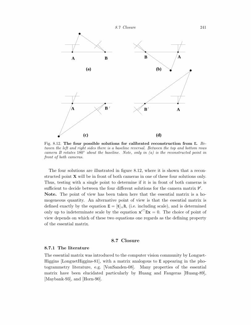
Fig. 8.12. The four possible solutions for calibrated reconstruction from E. Be-tween the left and right sides there is a baseline reversal. Between the top and bottom rowscamera B rotates 180◦ about the baseline. Note, only in (a) is the reconstructed point infront of both cameras.
The four solutions are illustrated in figure 8.12, where it is shown that a recon-structed point X will be in front of both cameras in one of these four solutions only.Thus, testing with a single point to determine if it is in front of both cameras issufficient to decide between the four different solutions for the camera matrix P′.Note. The point of view has been taken here that the essential matrix is a ho-mogeneous quantity. An alternative point of view is that the essential matrix isdefined exactly by the equation E = [t]×R, (i.e. including scale), and is determinedonly up to indeterminate scale by the equation x′>Ex = 0. The choice of point ofview depends on which of these two equations one regards as the defining propertyof the essential matrix.
8.7 Closure
8.7.1 The literature
The essential matrix was introduced to the computer vision community by Longuet-Higgins [LonguetHiggins-81], with a matrix analogous to E appearing in the pho-togrammetry literature, e.g. [VonSanden-08]. Many properties of the essentialmatrix have been elucidated particularly by Huang and Faugeras [Huang-89],[Maybank-93], and [Horn-90].
242 8 Epipolar Geometry and the Fundamental Matrix
The realization that the essential matrix could also be applied in uncalibratedsituations, as it represented a projective relation, developed in the early part of the1990s, and was published simultaneously by Faugeras [Faugeras-92a, Faugeras-92b],and Hartley et al. [Hartley-92a, Hartley-92c].
The special case of pure planar motion was examined by [Maybank-93] for theessential matrix. The corresponding case for the fundamental matrix is investigatedby Beardsley and Zisserman [Beardsley-95b] and Vieville and Lingrand [Vieville-95],where further properties are given.
8.7.2 Notes and exercises
(i) Fixating cameras. Suppose two cameras fixate on a point in space suchthat their principal axes intersect at that point. Show that if the imagecoordinates are normalized so that the coordinate origin coincides with theprincipal point then the F33 element of the fundamental matrix is zero.
(ii) Mirror images. Suppose that a camera views an object and its reflectionin a plane mirror. Show that this situation is equivalent to two views of theobject, and that the fundamental matrix is skew-symmetric. Compare thefundamental matrix for this configuration with that of: (a) a pure translation,and (b) a pure planar motion. Show that the fundamental matrix is auto-epipolar (as is (a)).
(iii) Show that if the vanishing line of a plane contains the epipole then the planeis parallel to the baseline.
(iv) Steiner conic. Show that the polar of xa intersects the Steiner conic Fs atthe epipoles (figure 8.10a). Hint, start from Fe = Fse + Fae = 0. Since elies on the conic Fs, then l1 = Fse is the tangent line at e, and l2 = Fae =[xa]×e = xa × e is a line through xa and e.
(v) Planar motion. It is shown by [Maybank-93] that if the rotation axis direc-tion is orthogonal or parallel to the translation direction then the symmetricpart of the essential matrix has rank 2. We assume here that K = K′. Thenfrom (8.12), F = K−>EK−1, and so
Fs = (F + F>)/2 = K−>(E + E>)K−1/2 = K−>EsK−1.
It follows from det(Fs) = det(K−1)2 det(Es) that the symmetric part of F isalso singular. Does this result hold if K 6= K′?
(vi) Any matrix F of rank 2 is the fundamental matrix corresponding to somepair of camera matrices (P, P′) This follows directly from result 8.14 since thesolution for the canonical cameras depends only on the rank 2 property of F.
(vii) Show that the 3D points determined from one of the ambiguous reconstruc-tions obtained from E are related to the corresponding 3D points determinedfrom another reconstruction by either (i) an inversion through the second

8.7 Closure 243
camera centre; or (ii) a harmonic homology of 3-space (see section A5.2-(p584)), where the homology plane is perpendicular to the baseline andthrough the second camera centre, and the vertex is the first camera centre.
(viii) Following a similar development to section 8.2.2, derive the form of the fun-damental matrix for two linear pushbroom cameras. Details of this matrixare given in [Gupta-97] where it is shown that affine reconstruction is possiblefrom a pair of images.