Episodic Liquidity Crises:

Cooperative and Predatory Trading

Bruce Ian Carlin1 Miguel Sousa Lobo2 S. Viswanathan3

August 30, 2005

1Fuqua School of Business, Duke University, bruce.carlin@duke.edu,

2Fuqua School of Business, Duke University, mlobo@duke.edu

3Fuqua School of Business, Duke University, viswanat@duke.edu

We thank Kerry Back, Ravi Bansal, Michael Brandt, Markus Brunnermeier,

Bhagwan Chowdry, Phil Dybvig, Simon Gervais, Milt Harris, Ming Huang, Ron

Kaniel, Pete Kyle, Leslie Marx, Uday Rajan, Ioanid Rosu, Ronnie Sadka, Duane

Seppi, Jim Smith, Curt Taylor, Huseyin Yildirim and seminar participants in

the 2005 World Congress of Economics, Duke Finance and Duke Economics

seminars, and the Indian School of Business for their comments.

1

Abstract

We develop a theoretical model to explain how episodic illiquidity can arise from

a breakdown in cooperation between traders and be associated with predatory

trading. In a multi-period framework, and with a continuous-time stage game

with an asset-pricing equation that accounts for transaction costs, we describe

an equilibrium where traders cooperate most of the time through repeated in-

teraction and provide ‘apparent liquidity’ to each other. Cooperation can break

down, especially when the stakes are high, and lead to predatory trading and

episodic illiquidity. Equilibrium strategies involving cooperation across markets

can cause the contagion of illiquidity.

2

Why is illiquidity rare and episodic? Pastor and Stambaugh (2003) detect only

14 aggregate low-liquidity months in the time period 1962-1999. The origin

of this empirical observation still remains a puzzle. In this paper, we develop

a theoretical model in which episodic illiquidity results from a breakdown in

cooperation between traders in the market and manifests itself in predatory

trading. This mechanism explains how sudden illiquidity appears, even in the

absence of observable market distress.

We develop a dynamic model of trading based on liquidity needs. During

each period, a liquidity event may occur in which a trader is required to liquidate

a large block of an asset in a relatively short time period. This need for liquidity

is observed by a tight oligopoly, whose members may choose to predate or

cooperate. Predation involves racing and fading the distressed trader to the

market, causing an adverse price impact for the trader1. Cooperation involves

refraining from predation and allows the distressed trader to transact at more

favorable prices. In our model, traders cooperate most of the time through

repeated interaction, providing ‘apparent liquidity’ to each other. However,

episodically this cooperation breaks down, especially when the stakes are high,

leading to opportunism and loss of this apparent liquidity.

The following quote provides a recent example of an episodic breakdown in1Predatory trading has been defined by Brunnermeier and Pedersen (2004) as trading that

induces and/or exploits another investor’s need to change their position. It is important todistinguish predatory trading from front-running. Front-running is an illegal activity in whicha specialist, acting as an agent of an investor, trades on his own account in the same directionas his client before he fulfills his client’s order. In this way, the specialist profits but violateshis legal obligation as an agent of the investor. Predatory activity occurs in the absence ofsuch a legal obligation.

3

cooperation between cooperative periods in the European debt market (New

York Times Sept. 15, 2004):

“...The bond sale, executed Aug. 2, caused widespread concern in

Europe’s markets. Citigroup sold 11 billion euros of European gov-

ernment debt within minutes, mainly through electronic trades, then

bought some of it back at lower prices less than an hour later, rival

traders say. Though the trades were not illegal, they angered other

bond houses, which said the bank violated an unspoken agreement

not to flood the market to drive down prices.” 2

This suggests that market participants cooperate, though there is episodic pre-

dation which leads to acute changes in prices. Note that predatory behavior can

involve either exploiting a distressed trader’s needs or inducing another trader

to be distressed.

There exists empirical evidence that cooperation affects price evolution and

liquidity in financial markets. Cocco, Gomes, and Martins (2003) detect ev-

idence in the Interbank market that banks provide liquidity to each other in

times of financial stress. They find that banks establish lending relationships

in this market to provide insurance against the risk of shortage or excess of

funds during the reserve maintenance period. Cooperation and reputation have

been documented to affect liquidity costs on the floor of the New York Stock

Exchange (NYSE). Battalio, Ellul, and Jennings (2004) show an increase in

liquidity costs in the trading days surrounding a stock’s relocation on the floor2On February 2, 2005 the Wall Street Journal reported that this predatory trading plan

was referred to as “Dr. Evil” by traders working at Citicorp.

4

of the exchange.3 They find that brokers who simultaneously relocate with the

stock and continue their long-term cooperation with the specialist obtain a lower

cost of liquidity, which manifests in a smaller bid-ask spread.4

In our predatory stage game, each trader faces a differential game with other

strategic traders, that is a dynamic game in continuous time. Our stage game

is related to the model by Brunnermeier and Pedersen (2004), but distinct in

many respects. Because we use a pricing equation that accounts for the effect

of trading pressure on price, the strategic traders, as a group, suffer surplus

loss when predatory trading is present. This surplus loss motivates the traders

to cooperate and provide liquidity to each other in our repeated game. In the

formulation by Brunnermeier and Pedersen, no transaction costs are incurred

in the equilibrium solution and all gains by the predators are exactly offset by

losses by distressed traders, so that there would be no feasible Pareto improve-

ment in a repeated game.5 6 In the equilibrium of our stage game, traders

‘race’ to market, selling quickly in the beginning of the period, at an exponen-

tially decreasing rate. Also in equilibrium, predators initially race the distressed3This is an exogenous event that changes long-run relationships between brokers and the

specialist.4Other articles in this literature include Berhardt, Dvoracek, Hughson, and Werner 2004;

Desgranges and Foucault 2002; Reiss and Werner 2003; Ramadorai 2003; Hansch, Naik, andViswanathan 1999; Massa and Simonov 2003

5There are other substantial differences between the models. Brunnermeier and Pedersenimpose exogenous holding limits ([−x, x]) for traders, whereas we do not make this restriction.Our model involves a stochastic price process, while in Brunnermeier and Pedersen the assetpricing relationship is deterministic. Finally note that Brunnermeier and Pedersen’s modelpredicts “price-overshooting”, whereas our model does not. However, this is a consequenceof, in our stage game model, all traders having an identical time horizon. If we relax this asin Brunnermeier and Pedersen to allow predators a longer horizon, price overshooting is alsoobserved in our model.

6Attari, Mello, and Ruckes (2004) also describe predatory trading behavior with a two-period model. They show that predators may even lend to others that are “financially fragile”because they can obtain higher profits by trading against them for a longer period of time. Ourpaper generalizes their model in a multi-period framework, with each period in a continuous-time setting.

5

traders to market, but eventually ‘fade’ them and buy back. This racing and

fading behavior is well-known in the trading industry and has been previously

modelled by Foster and Viswanathan (1996). The associated trading volumes

are also consistent with the U-shaped daily trading volume seen in financial

markets.

We model cooperation by embedding the predatory stage game in a dynamic

game. We first consider an infinitely-repeated game in which the magnitude

of the liquidity event is fixed. In this framework, there exists an extremal

equilibrium which is Pareto superior for the traders. We show that traders

are more likely to cooperate in markets where assets are thinly-traded (i.e.,

thin corporate bond issues, exotic options, credit derivatives) and in markets

with low transaction costs. Further, we show that the need for liquidity over

time needs to be sufficiently symmetric between the traders for cooperation

to be maintained. The existence of asymmetric distress probabilities leads to

abandonment of cooperation in equilibrium.

We extend the model to episodic illiquidity by allowing the exogenous mag-

nitude of the liquidity event in the repeated game to be stochastic. Given such

stochastic liquidity shocks, we provide predictions as to the magnitude of liq-

uidity event required to trigger liquidity crises and describe how a breakdown

in cooperation leads to price volatility. Finally, we allow for multimarket con-

tact in the stochastic version of our dynamic game. This increases cooperation

across markets, but leads to contagion of predation and liquidity crises across

6

all markets.7

We note a few of the empirical implications of our model. First, our model

predicts that non-anonymous markets should be stable most of the time with

high ‘apparent’ liquidity, but will experience illiquidity in an episodic fashion.

This fact is consistent with the observed rareness of liquidity events in financial

markets (Pastor and Stambaugh 2003; Gabaix, Krishnamurthy, and Vigneron

2004). Second, in markets with thin issues and low transaction costs, the disap-

pearance of apparent liquidity should be the most marked when these episodes

occur. Third, occasions where one player faces extreme financial distress are

associated with periods of reduced liquidity. Finally, our model suggests that

illiquidity is usually observed across markets (i.e., contagion occurs), and not

in isolation.

The paper is organized as follows. Section 1 introduces the pricing relation-

ship and sets up the stage game. We derive closed-form solutions for the trading

dynamics and quantify the surplus loss due to competitive trading. Section 2

uses the stage game with one predator and one distressed trader as a basis and

provides the solution to the supergame with the magnitude of the liquidity event

fixed. Section 2 also models the relationship between insiders and outsiders in

these markets. Section 3 models episodic illiquidity by having the magnitude

of the liquidity shocks be stochastic. Contagion of illiquidity across markets7Our mechanism for contagion is different from that of Brunnermeier and Pedersen (2004).

The contagion in Brunnermeier and Pedersen (2004) is caused by a wealth effect. As pricesin the market drop, additional traders are induced into a state of distress and a market-widesell-off is observed. While this is a reasonable description of contagion during market distress,it does not explain why low-liquidity periods occur even in the absence of market downturns(Pastor and Stambaugh 2003). Our model predicts that contagion of illiquidity can occur inthe absence of wealth effects.

7

is also addressed in this section. Section 4 concludes. Appendix A contains

proofs. While the stage-game solution in Section 1 is based on the equilib-

rium over open-loop strategies, in Appendix B we consider the equilibrium over

closed-loop strategies and argue that results are not qualitatively different as a

consequence.

1 Trading and Predation

1 A Asset price model

The economy consists of two types of participants. The strategic traders, i =

1, 2, ..., n, are risk-neutral and maximize trading profits. These traders form a

tight oligopoly over order flow in financial markets. Large traders are usually

present in markets as proprietary trading desks, trading both on their own

accounts as well as for others. The strategic traders observe the order flow and

have inside information regarding transient liquidity needs within the market.

They attempt to generate profits through their ability to forecast price moves,

and to affect asset prices.

The other players are the long-term investors who form the competitive

fringe. The long-term investors usually trade in the interest of mutual funds

or private clients and exhibit a less aggressive trading strategy. Long-term in-

vestors are more likely to take a “buy and hold strategy”, limit the number

of transactions that they undertake, and avoid taking over-leveraged positions.

The long-term investors trade according to fundamentals. The primary differ-

8

ence between the two types of traders is that the long-term investors are not

aware of transient liquidity needs in the economy.

There exist a risk-free asset and a risky asset, traded in continuous-time.

The aggregate supply S > 0 of the risky asset at any time t is divided between

the strategic investors’ holdings Xt and the long-term investors’ holdings Zt

such that S = Xt + Zt. The return on the risky asset is stochastic. The yield

on the risk-free asset is zero.

The asset is traded at the price

Pt = Ut + γXt + λYt, (1)

where

dXt = Ytdt, (2)

and Ut is the stochastic process dUt = σ(t, Ut)dBt, with Bt some one-dimensional

Brownian motion on (Ω,F , P ).

A similar pricing relationship was previously derived by Vayanos (1998),

and as well as by Gennotte and Kyle (1991) who show that it arises from the

equilibrium strategies between a market maker and an informed trader when

the position of the noise traders follows a smoothed Brownian motion. Likewise,

Pritsker (2004) obtains a similar relationship for the price impact of large trades

when institutional investors transact in the market. 8 9

8Directly linking trading pressure and price distinguishes our model from Brunnermeierand Pedersen (2004), where transaction costs are modeled via an exogenous parameter A (themaximum trading rate at which transaction costs are avoided), which does not directly affectprices in the market. This results in there being no surplus to be gained from cooperation.

9Further motivation for our use of this pricing relationship are the empirical and theo-retical studies that link trading pressure and asset prices (Keim and Madhavan 1996; Kaul,Mehrotra, and Morck 2000; Holthausen, Leftwich, and Mayers 1990; Chan and Lakonishok1995; Bertsimas and Lo 1998; Fedyk 2001; DeMarzo and Urosevic 2000; Almgren and Chriss2000; Almgren and Chriss 1999; Huberman and Stanzl 2000).

9

The pricing equation is composed of three parts. Ut represents the expected

value of future dividends and is modeled as a martingale stochastic diffusion

process. The diffusion does not include a drift term, which is justified by the

short-term nature of the events modeled. The results described here can be

derived with the inclusion of a drift term in the diffusion, but with considerable

loss in clarity of exposition.10

The second and third terms decompose the effect of liquidity on the asset

price into permanent and temporary components. The effect of liquidity risk on

asset prices has been studied by Acharya and Pedersen (2005) and others, and

a related decomposition into short- and long-term effects has been considered

by Sadka (2005).

In the second term, Xt is the inventory variable in the economy, which

measures the amount of the asset that the strategic traders hold at time t.

As Xt increases, the supply available to the long-term investors decreases and

the price at which they can access the asset increases. The model parameter

γ measures the permanent liquidity effects of trading. That is, it measures

the change in price of the asset which is independent of the rate at which the

asset is traded. Note that the level of asymmetric information in an asset is

likely to be a major determinant of γ, as demand for the asset will then play a

more important role in price formation. For instance, we expect a AAA-rated10More precisely, the assumption is that the difference between the drift coefficient and the

continuous-time discount factor is zero. For the multi-period game which we will later discuss,the assumption is that T is relatively small, that is the distress and predation events developover short periods of time, and the discounting over each period is therefore not significant.The period-to-period discount factor is then also close to one. Since each period is short,the multi-stage game will consist of many short periods, where the probabilities of a playerbeing distressed in any given period are small, so that the period-to-period discount factor issignificant to the problem.

10

corporate bond to have lower asymmetric information associated with it then a

B-rated bond. In our model, the AAA-rated bond should then have a lower γ

than the B-rated bond. Likewise, an asset with concentrated ownership should

have a higher level of asymmetric information (and therefore a higher γ) than

an asset with a more dispersed ownership structure. For an asset with more

asymmetric information, the market will more strongly adjust the asset price

based on the net change in the supply of the asset.

The third term measures the instantaneous, reversible price pressure that

occurs as a result of trading. Yt is the aggregate rate of trading of the asset

by the strategic traders. The faster the traders sell, the lower a price they will

realize. This leads to surplus loss effects, which are discussed in the following

subsections. The price-impact parameter λ measures the temporary, reversible

asset price change that occurs during trading. Trading volume, concentration

of ownership, and shares outstanding are all likely to play a role in the level of

λ.

In the following sections, we use γ and λ to predict which securities in the

market are more prone to predatory and to cooperative trading, and to episodic

illiquidity. We show that the magnitude of the ratio γλ is the key determinant

of predatory or cooperative trading behavior.

1 B Stage Game: Trading Dynamics

The stage game that we consider is a game of complete information. Many assets

that are prone to illiquidity are traded in non-anonymous markets in which a

11

few large dealers dominate order flow. Further, roughly half of the trading

volume at the New York Stock Exchange is traded in blocks over 10, 000 shares

(Seppi 1990) and much of that occurs in the “upstairs” market, which is non-

anonymous. As a result, the liquidity needs of large traders are usually observed

quickly by others.

To understand the intuition behind this choice of structure for the game,

consider a thinly-traded corporate bond issue that is traded by a small number

of broker-dealers. Trading occurs either by direct negotiation over the phone,

or by “sunshine” trading in which a mini-auction is held. The players are well-

known to each other because they deal repeatedly with each other. Their trading

habits and strategies are common knowledge.11 When one trader needs to trade

a large block of shares of an asset, this need is observed by others in the market

and the optimal trading strategies solve a game of complete information.

In the stage game, strategic traders are either distressed or are predators. A

liquidity event occurs at time t = 0, whereby the distressed traders are required

buy or sell a large block of the asset ∆x in a short time horizon T (say, by the

end of the trading day). Forced liquidation usually arises because of the need to

offset another cash-constrained position such as an over-leveraged position, or it

occurs as a result of a risk management maneuver. The predators are informed

of the trading requirement of the distressed traders and compete strategically

in the market to exploit the price impact of the distressed trader’s selling. For11A particularly clear example of this is the Mortgage market developed by Salomon Broth-

ers. Once this market was established and profitable, many of Salomon’s mortgage traderswere hired by other investment banks to run their mortgage desks. As a consequence, thetrading habits of all of the desks were especially well-known to each other.

12

clarity of exposition, we assume that the opportunistic traders must return to

their original positions in the asset by the end of the trading period, and that

the distressed traders are informed of this requirement.12 Further, we assume

that, except for their trading targets, all strategic traders are identical. That is,

the only difference between the two types of strategic traders is that the trading

target for the distressed traders is ∆x, and zero for the predatory traders.

At the start of the stage game, every trader chooses a trading schedule (Y it )

over the period [0, T ] to maximize their own expected value, assuming the other

traders will do likewise. Subject to their respective initial and terminal holding

constraints, they solve the following dynamic program

maximize E∫ T

0−PtY

it dt

subject to Xi0 = x0i

XiT = xTi

(3)

by choosing a trading function Y it . The expectation is over the Brownian mo-

tion’s measure. We restrict our analysis of equilibrium solutions of this differen-

tial game to open-loop Nash equilibria, in which each trader chooses ex ante a

time-dependent trading strategy that is the best response to the other traders’

expected actions. As noted in proof in appendix, convexity ensures that the

problem is well-posed.13 The equilibrium solution is weakly time consistent.12A variation on this model would be to allow the opportunistic traders to trade over a longer

time period than the distressed traders. The solution for such a model is similar. However,the predatory trader will now choose what position to have by the end of the distressedseller’s deadline. This choice is made by maximizing the expected value from trading over thedistressed seller’s period, plus the expected value from selling the position at the end of thatperiod at a constant rate over the additional time. (See also Footnote 5.)

13Convexity ensures that any solution is identical almost everywhere to the one given here(i.e., has the same integrals). Further restrictions can be imposed on the Yt if desired, such as

13

The solution to the subproblem over the inteval [t1, T ] (with initial conditions

as given by the solution of the [0, T ]-problem at time t1) is the truncation of the

[0, T ]-solution over that sub-interval.14 Once trading is underway, and at any

given point in the trading schedule, no trader has a rational reason to deviate

from the chosen trading function, as long as other traders do not deviate in re-

sponse (either because they are able to credibly commit, or because they cannot

observe the first player’s deviation). Traders are not able to benefit from alter-

ing their trading strategy part-way through the game, as long as other players

stick to their strategies.15

The following result outlines the Nash equilibrium solution for the traders.

This formulation will serve a basis for deriving the equilibrium strategies when

several distressed traders are present without opportunism and when there are

both opportunistic and distressed traders present in the economy. It will also

allow for analysis of trader surplus, which will motivate cooperation between

traders in the repeated game.

Result 1 (General Solution) Consider N traders that choose a time-dependent

trading rate Y it to solve the optimization problem in Equation 3, subject to the

being of bounded variation. Since the traders solve an open-loop problem, Y it can be defined

as a functional rather than a process (by the same argument randomized solutions can beexcluded, and the Brownian motion is not in the information set). Alternatively, smoothnesscan be ensured by defining the solution to the continuous-time problem as the limit of thesolutions to a sequence of discrete-time problems, which is the approach we will use to analyzethe closed-loop version of the problem in Appendix B.

14See Theorem 6.12 in Basar and Olsder (1999) and related discussion.15In Appendix B we analyze closed-loop strategies, where players take into account the other

players’ response functions and are able to change their trading strategies part-way throughthe game. Solutions to the closed-loop problem are strongly time consistent. Our analysis,which we also confirmed with numerical experiments, suggests that the equilibrium tradingstrategies are qualitatively similar, and that the welfare loss is somewhat higher than what weobtain with open-loop strategies in Section 1 C. In the repeated-game analysis of Section 2,this would make the players more likely to cooperate.

14

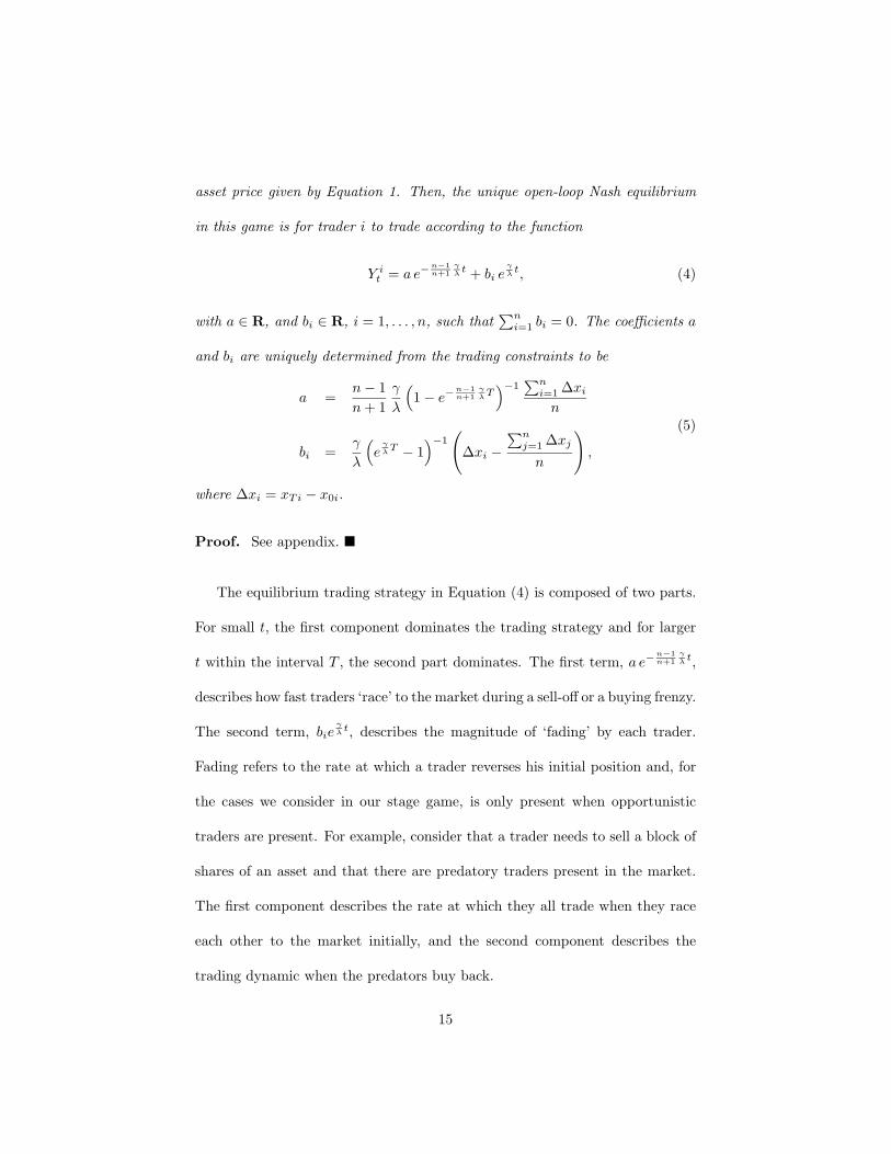
asset price given by Equation 1. Then, the unique open-loop Nash equilibrium

in this game is for trader i to trade according to the function

Y it = a e−

n−1n+1

γλ t + bi e

γλ t, (4)

with a ∈ R, and bi ∈ R, i = 1, . . . , n, such that∑n

i=1 bi = 0. The coefficients a

and bi are uniquely determined from the trading constraints to be

a =n − 1n + 1

γ

λ

(1 − e−

n−1n+1

γλ T

)−1∑n

i=1 ∆xi

n

bi =γ

λ

(e

γλ T − 1

)−1(

∆xi −∑n

j=1 ∆xj

n

),

(5)

where ∆xi = xTi − x0i.

Proof. See appendix.

The equilibrium trading strategy in Equation (4) is composed of two parts.

For small t, the first component dominates the trading strategy and for larger

t within the interval T , the second part dominates. The first term, a e−n−1n+1

γλ t,

describes how fast traders ‘race’ to the market during a sell-off or a buying frenzy.

The second term, bieγλ t, describes the magnitude of ‘fading’ by each trader.

Fading refers to the rate at which a trader reverses his initial position and, for

the cases we consider in our stage game, is only present when opportunistic

traders are present. For example, consider that a trader needs to sell a block of

shares of an asset and that there are predatory traders present in the market.

The first component describes the rate at which they all trade when they race

each other to the market initially, and the second component describes the

trading dynamic when the predators buy back.

15

Note that the constant a in Equation (5) is a function of the average trading

target over all traders. All traders race to the market in similar fashion, based

on the common knowledge of their overall trading target. Towards the end of the

period, traders ‘fade’ based on their particular trading targets. The constants bi

are a function of how each trader’s trading target is different from the average.

A ‘distressed trader’, in the sense that he has a higher-than-average trading

target, towards the end of the period will trade in the same direction as the

racing. A ‘predatory trader’, in the sense that she has a smaller-than-average

trading target, will ‘fade’ in the opposite direction, that is reverse the direction

in which she is trading.

For a single trader, the equations reduce to Y 1t = ∆x1

T , that is to a trading

rate schedule. To develop more intuition regarding Result 1, we evaluate Equa-

tion (4) for special cases, which we will use when we consider the repeated game

in Sections 2 and 3.

Case 1 (Symmetric Distressed Traders). First, consider the optimal trad-

ing policy when a trader has monopoly power and buys or sells in the absence

of other strategic traders. For n = 1, the optimal trading policy (4) for a single

trader is to trade at a constant rate, Yt = a = ∆xT , where ∆x is the block of

shares that the trader needs to buy or sell.

Now, consider n symmetric traders, each needing to sell an identical amount

of shares ∆xn . From Equation (4), the unique equilibrium trading strategy is

Y it = a e−

n−1n+1

γλ t, i = 1, . . . , n, (6)

16

where a is as in (5) with∑n

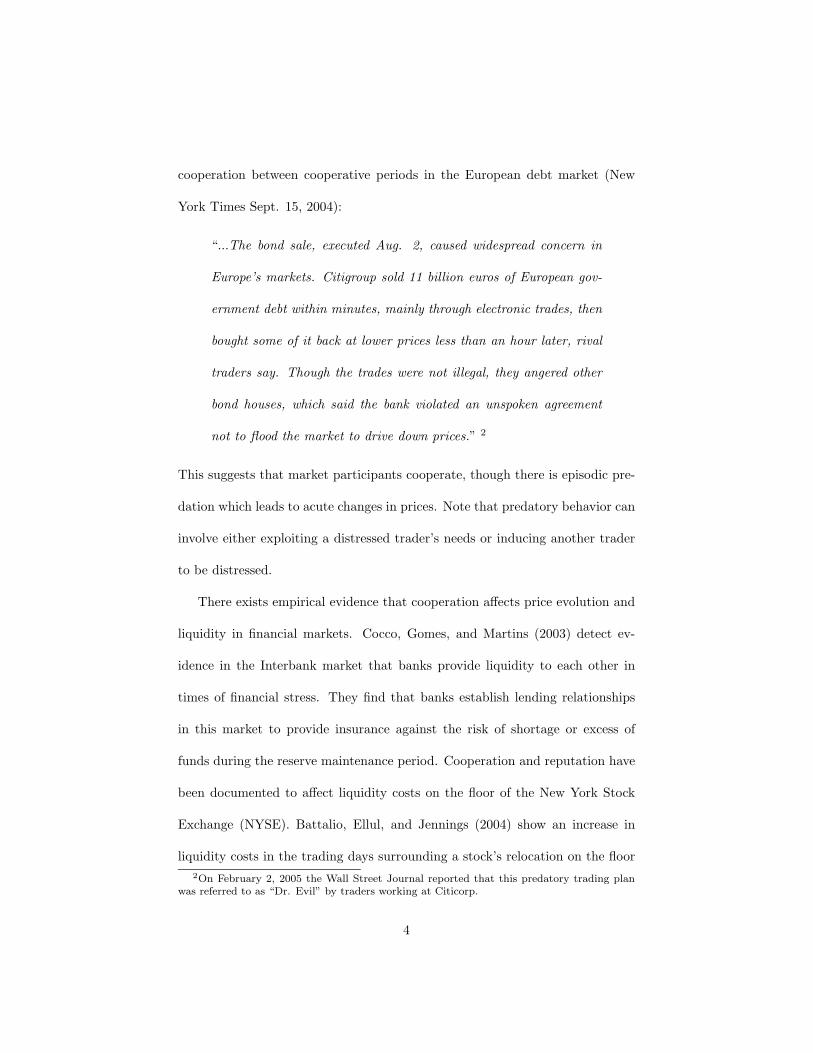
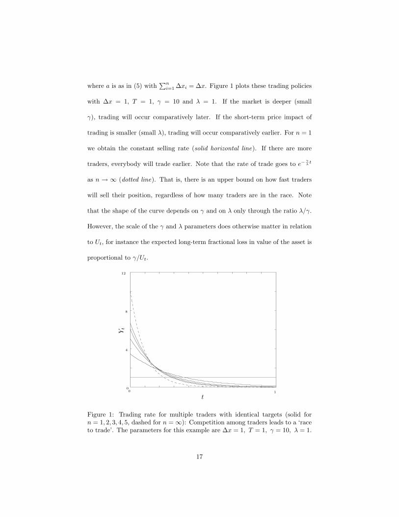
i=1 ∆xi = ∆x. Figure 1 plots these trading policies

with ∆x = 1, T = 1, γ = 10 and λ = 1. If the market is deeper (small

γ), trading will occur comparatively later. If the short-term price impact of

trading is smaller (small λ), trading will occur comparatively earlier. For n = 1

we obtain the constant selling rate (solid horizontal line). If there are more

traders, everybody will trade earlier. Note that the rate of trade goes to e−γλ t

as n → ∞ (dotted line). That is, there is an upper bound on how fast traders

will sell their position, regardless of how many traders are in the race. Note

that the shape of the curve depends on γ and on λ only through the ratio λ/γ.

However, the scale of the γ and λ parameters does otherwise matter in relation

to Ut, for instance the expected long-term fractional loss in value of the asset is

proportional to γ/Ut.

00

4

8

12

1

Yt

t

Figure 1: Trading rate for multiple traders with identical targets (solid forn = 1, 2, 3, 4, 5, dashed for n = ∞): Competition among traders leads to a ‘raceto trade’. The parameters for this example are ∆x = 1, T = 1, γ = 10, λ = 1.

17

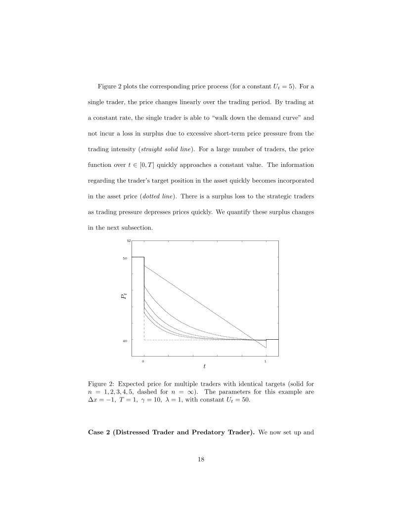
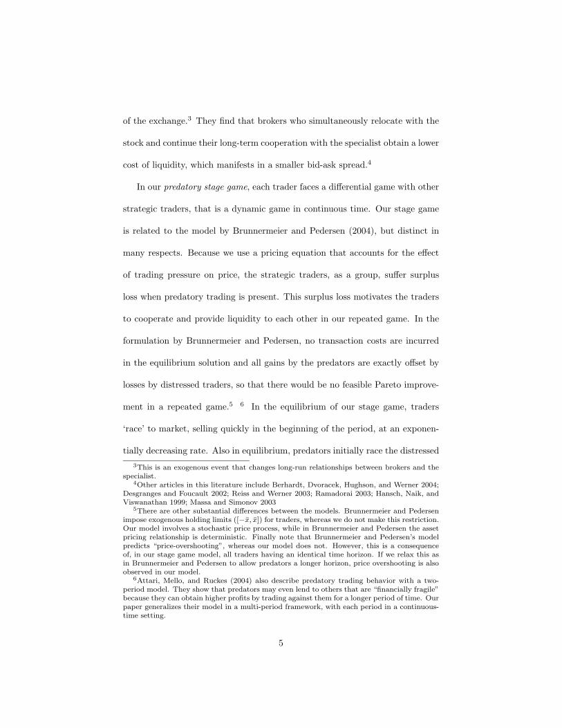
Figure 2 plots the corresponding price process (for a constant Ut = 5). For a

single trader, the price changes linearly over the trading period. By trading at

a constant rate, the single trader is able to “walk down the demand curve” and

not incur a loss in surplus due to excessive short-term price pressure from the

trading intensity (straight solid line). For a large number of traders, the price

function over t ∈ [0, T ] quickly approaches a constant value. The information

regarding the trader’s target position in the asset quickly becomes incorporated

in the asset price (dotted line). There is a surplus loss to the strategic traders

as trading pressure depresses prices quickly. We quantify these surplus changes

in the next subsection.

52

40

50

0 1

Pt

t

Figure 2: Expected price for multiple traders with identical targets (solid forn = 1, 2, 3, 4, 5, dashed for n = ∞). The parameters for this example are∆x = −1, T = 1, γ = 10, λ = 1, with constant Ut = 50.

Case 2 (Distressed Trader and Predatory Trader). We now set up and

18

analyze the two-player predatory stage game, which will form the basis for the

infinitely-repeated game in Section 2. Consider that there exists one distressed

and one opportunistic trader. Each trader chooses a trading schedule (Y dt and

Y pt ) over the period [0, T ] to maximize his own expected value, assuming the

other trader will do likewise. From Result 1, the unique equilibrium trading

policies are

Y dt = a e−

13

γλ t + b e

γλ t

Y pt = a e−

13

γλ t − b e

γλ t,

(7)

where

a =γ

6λ

(1 − e−

13

γλ T

)−1

∆x, b =γ

2λ

(e

γλ T − 1

)−1

∆x. (8)

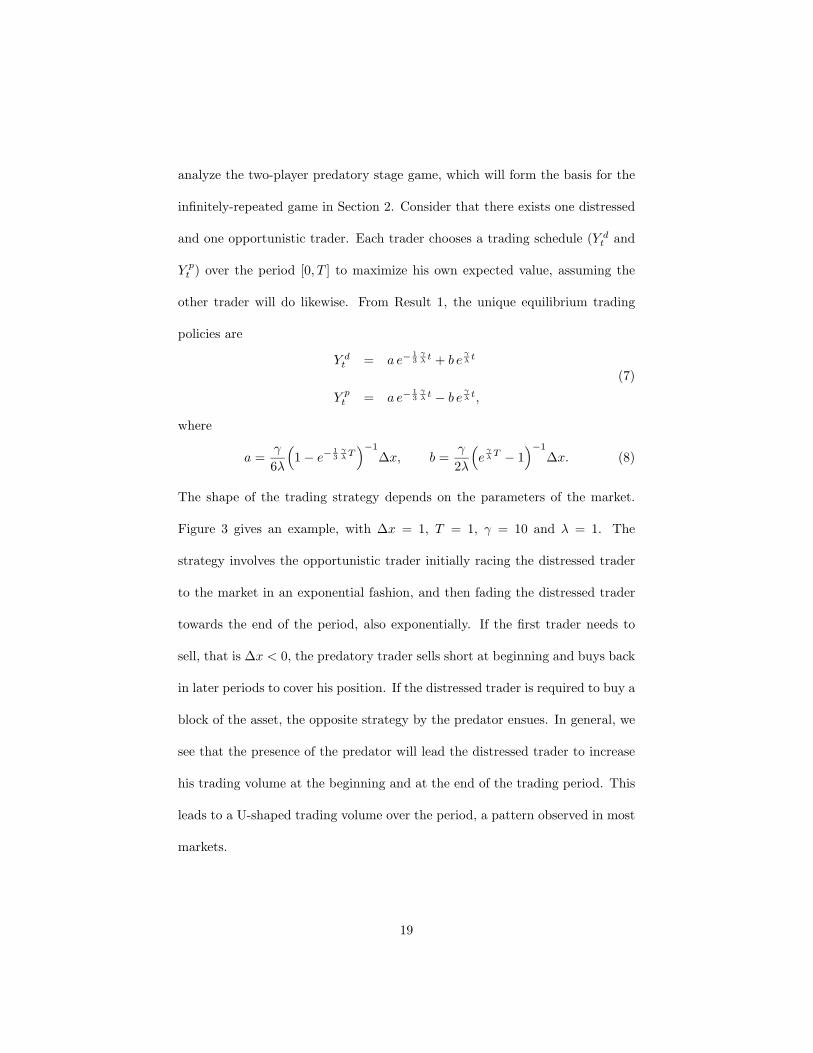
The shape of the trading strategy depends on the parameters of the market.

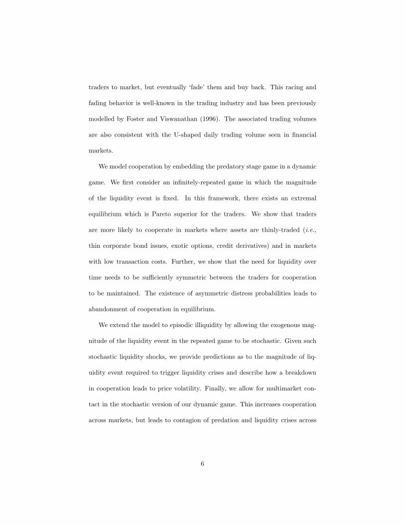
Figure 3 gives an example, with ∆x = 1, T = 1, γ = 10 and λ = 1. The

strategy involves the opportunistic trader initially racing the distressed trader

to the market in an exponential fashion, and then fading the distressed trader

towards the end of the period, also exponentially. If the first trader needs to

sell, that is ∆x < 0, the predatory trader sells short at beginning and buys back

in later periods to cover his position. If the distressed trader is required to buy a

block of the asset, the opposite strategy by the predator ensues. In general, we

see that the presence of the predator will lead the distressed trader to increase

his trading volume at the beginning and at the end of the trading period. This

leads to a U-shaped trading volume over the period, a pattern observed in most

markets.

19

0

0

-4

4

1

y i

t

Figure 3: One trader with position target (solid) and one ‘opportunistic’ trader(dashed). The parameters for this example are ∆x = 1, T = 1, γ = 10, λ = 0.1.

1 C Stage Game: Surplus Effects

Based on the trading dynamics in Section 1 B, we quantify the surplus changes

that occur when traders race to market and when predatory trading occurs.

The surplus values that we derive will be used in the following sections.

First, consider the expected value for a single trader with monopoly power.

Given the price (1) and the optimal trading rate Yt = ∆xT , the expected value

for the single trader is easily seen to be

V1 = −U0 ∆x −(

γ

2+

λ

T

)∆x2. (9)

This is the trader’s first best when there are no other competing traders informed

of the trader’s trading requirement ∆x. The costs due to short-term trading

pressure on the price are minimized. When other players trade strategically at

20

the same time, the value that the trader can derive is strictly lower that V1.

We will also see that when multiple traders compete in a sell-off or if there is

predatory trading, the total surplus available to all traders is decreased.

Define Vn as the total expected value for the strategic traders when n traders

play this game and define ∆Vn as the change in total surplus that occurs com-

pared to the expected value when all participants trade at a constant rate (V1).

The following result provides expressions for Vn and ∆Vn, and shows that the

loss in surplus is increasing with the number of traders. It will lay some ground-

work for the surplus results for the case where there is a distressed and a preda-

tory trader, and is also of interest on its own for the monotonicities.

Result 2 (Expected Total Surplus and Loss for Multiple Traders) The total

expected value for n traders with a combined trading target ∆x is

Vn = − U0 ∆x − γ

2

(1 +

n − 1n + 1

· en−1n+1

γλ T + 1

en−1n+1

γλ T − 1

)∆x2. (10)

The expected loss in total surplus from competition is

∆Vn = V1 − Vn = γ

(12· n − 1n + 1

· en−1n+1

γλ T + 1

en−1n+1

γλ T − 1

− 1γλT

)∆x2. (11)

∆Vn is positive, monotonic increasing in γ, T and n, and monotonic decreasing

in λ.

Proof. See appendix.

Now we apply Result 2 to the two-trader case and derive a surplus result

that we will use in Section 2. We define V2 as the total expected value for the

strategic traders when two traders play this game, and we define Vd and Vp as

21

the expected values to the distressed trader and to the opportunistic trader (as

defined in Section 1 B). Likewise, we define ∆V2 as the change in surplus that

occurs compared to the expected value V1 that is obtained when the participants

trade at a constant rate.

Result 3 (Expected Total Surplus and Loss for Two Traders) The total expected

value for the distressed trader and the predatory trader is

V2 = Vd + Vp = − U0 ∆x − γ

3· 2e

13

γλ T − 1

e13

γλ T − 1

∆x2. (12)

The expected value is divided as

Vd = −U0 ∆x − γ

65e

γλ T + e

23

γλ T + e

13

γλ T − 1

eγλ T − 1

∆x2,

Vp =γ

6· e

23

γλ T − 1

e23

γλ T + e

13

γλ T + 1

∆x2.

(13)

The expected loss due to predation for the distressed trader is

∆Vd = V1 − Vd = γ

(16· 2e

γλ T + e

23

γλ T + e

13

γλ T + 2

eγλ T − 1

− 1γλT

)∆x2, (14)

and the expected loss from predation in total surplus for the strategic traders is

∆V2 = V1 − V2 = γ

(16· e

13

γλ T + 1

e13

γλ T − 1

− 1γλT

)∆x2. (15)

Vp is monotonically increasing in γ and in T , and monotonically decreasing in

λ.

The ratio of gains to the predator to the losses to the distressed trader, Vp

∆Vd,

is monotonically decreasing in γ and in T , monotonically increasing in λ, and is

bounded (tightly) by 45 >

Vp

∆Vd> 1

2 . Note that it follows from Result 2 that ∆V2

is positive, monotonic increasing in γ and T , and monotonic decreasing in λ.

From the monotonicity of Vp it also follows that ∆Vd = ∆V2 +Vp is monotonic.

22

Proof. See appendix.

From the solutions for the rate of trading, we can see that a larger γλ ratio

(less market depth and lower transaction costs) creates conditions for more ag-

gressive predation, in the sense that trading will be relatively more concentrated

at the beginning and at the end of the period. Racing is more aggressive, and

fading occurs closer to the end of the trading period.

Since Vp

∆Vdis bounded in the interval [12 , 4

5 ], the losses to the distressed trader

are strictly higher than the gains by the predator. Even though the monotonicity

of Vp implies that market conditions that lead to more aggressive predation

(larger γ or lower λ or both) will lead to more gains from predation, since Vp

∆Vd

decreases in γ and increases in λ, the losses to the distressed trader grow faster

than the gains to the predator. In this one-shot stage game, this represents a

significant surplus loss to the traders.16 In a dynamic setting, which we model

in the next section, if both traders have a possible liquidity need in each period,

there exists a potential for Pareto improvement if the traders can cooperate.

As we will see, ∆x, λ, and γ are important determinants in predicting whether

cooperation is possible.

Finally, for some insight into the magnitude of the available Pareto improve-

ment, consider the limit case when λ γT . These are the conditions under

which predation is most aggressive, that is when racing and fading are fastest

as a consequence of the low transaction costs. Takingh the limit λ → 0 (which,

16In our stage game, we do not allow for ex-post renegotiation. Surplus losses are commonin many models in non-cooperative game theory (i.e., Prisoner’s Dilemma and CentipedeGame) and motivate cooperation in repeated play.

23

by change of units, is immediately seen to be equivalent to T → ∞), L’Hopital’s

rule yields for the overall surplus loss, the distressed trader’s losses from preda-

tion, and the predator’s gains:

∆V2 → γ

6∆x2,

∆Vd → γ

3∆x2,

Vp → γ

6∆x2.

(16)

In the limit, under market conditions that favor the most aggressive predation,

the predator gains (Vp) half of what the distressed trader loses (∆Vd). This is

the lower bound for Vp

∆Vd.

2 Cooperation and Liquidity (Repeated Game)

The repeated game is based on the case in which there are two strategic traders,

as well as a large number of long-term investors. Each player faces a common

discount factor δ, and the common asset price determinants U0, γ, and λ. At

the beginning of each stage, nature moves first, assigns a type to each of the

traders and both traders know each other’s type in each round.17 In each round,

each trader, with probability pi i = 1, 2, must liquidate a large position of size

∆x, and may act as a predator with probability 1 − pi. We assume that the

distress probabilities p1 and p2 are mutually independent and the magnitude of

the shock ∆x is constant. An alternative approach, which we take in Section 3,17In models of implicit collusion under imperfect information (Green and Porter 1984;

Abreu, Pearce, and Stacchetti 1986), players never deviate in equilibrium, but enter punish-ment phases because of exogenous price changes. Our game is one of complete information,where deviations cannot arise from such exogenous factors. This allows for a simpler modelwich captures the key issues of interest, namely how apparent liquidity arises from incentivesto cooperate.

24

is to model ∆x as a random variable, and compute the value of the supergame

by expectation over future liquidity events.

In each time period one of the following four events occurs: neither of the

two players is distressed, with probability (1 − p1)(1 − p2); the second player

is distressed but the first is not, with probability (1 − p1)p2; the first player is

distressed but the second is not, with probability p1(1 − p2); both players are

distressed, with probability p1p2. The four probabilities add to one. Coopera-

tion is possible when either there exists one predator and one distressed trader

(with probability p1 + p2 − 2p1p2), or when both players are distressed (with

probability p1p2). If only one of the players is distressed and needs to liquidate

a position, cooperation involves the other refraining from engaging in predatory

trading. If both traders are distressed, cooperation involves both traders selling

at a constant rate and refraining from racing each other to the market for their

own gain.

Cooperation provides the players with the ability to quickly sell large blocks

of shares, for the price that would be obtained by selling them progressively over

time. That is, while cooperation is ongoing, the distressed trader is allowed to

‘ride down’ the demand curve, rather than having the information regarding

the trading target quickly incorporated into the asset price, ahead of most of

his trading. In this sense, that large blocks of shares can be moved for a better

price, the market will appear more liquid. It will also avoid the volatility and

potential instability from the large trading volume peaks associated with the

racing and fading.

25

The punishment strategy considered is a trigger strategy in the spirit of

Dutta and Madhavan (1997) and Rotemberg and Saloner (1986). That is, for

a given discount factor δ, the value of a perpetuity of cooperation must exceed

a one-time deviation plus a perpetuity of non-cooperation. Based on the Folk

Theorem, a convex set of subgame perfect Nash equilibria may exist in which

intermediate levels of cooperation occur. For clarity of exposition, we focus on

the extremal equilibrium in which intermediate levels do not exist.

The purpose of this set-up is to evaluate when the traders will abandon

a cooperative effort, thereby leading to illiquidity in the market. Compara-

tive statics regarding the nature of this cooperative effort can be generated by

comparing the level of δ required in different scenarios. Given any particular

punishment scheme, such as the more complicated penal codes in Abreu 1988,

such a critical δ can be derived. For this analysis, we do not allow the players to

change punishment schemes to achieve cooperation. Therefore, we focus on trig-

ger stratgies because they lead to the same economic results, while maintaining

clarity of the model.

The following result describes the extremal equilibrium of our repeated game

with fixed liquidity needs (∆x) in each period, using a trigger strategy. Refer

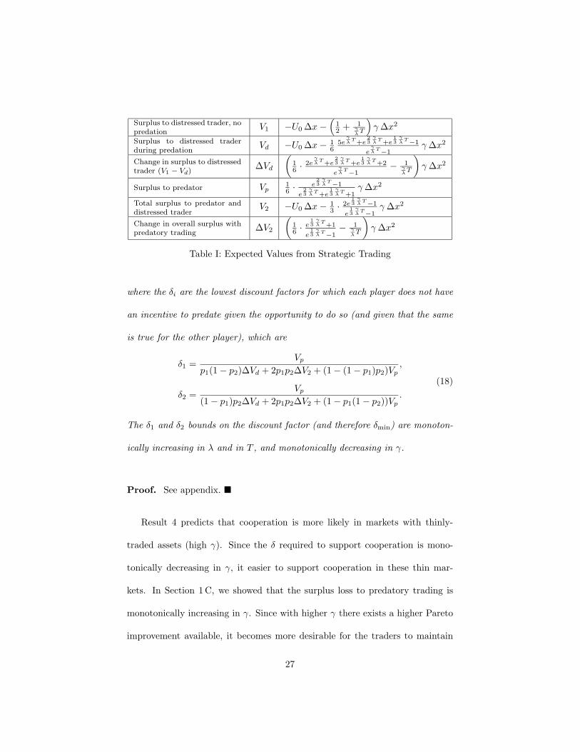
to Table I for the expected values derived in Section 1.

Result 4 (Repeated Game with Two Symmetric Traders) Define the expected

values as in Section 1. When a trigger strategy (punishment strategy) is used,

the discount factor required to support collusion is

δ ≥ δmin = max δ1, δ2 , (17)

26

Surplus to distressed trader, nopredation

V1 −U0 ∆x −(

12 + 1

γλ T

)γ ∆x2

Surplus to distressed traderduring predation

Vd −U0 ∆x − 16

5eγλ

T +e23

γλ

T +e13

γλ

T −1

eγλ

T −1γ ∆x2

Change in surplus to distressedtrader (V1 − Vd)

∆Vd

(16 · 2e

γλ

T +e23

γλ

T +e13

γλ

T +2

eγλ

T −1− 1

γλ T

)γ ∆x2

Surplus to predator Vp16 · e

23

γλ

T −1

e23

γλ

T +e13

γλ

T +1γ ∆x2

Total surplus to predator anddistressed trader

V2 −U0 ∆x − 13 · 2e

13

γλ

T −1

e13

γλ

T −1γ ∆x2

Change in overall surplus withpredatory trading

∆V2

(16 · e

13

γλ

T +1

e13

γλ

T −1− 1

γλ T

)γ ∆x2

Table I: Expected Values from Strategic Trading

where the δi are the lowest discount factors for which each player does not have

an incentive to predate given the opportunity to do so (and given that the same

is true for the other player), which are

δ1 =Vp

p1(1 − p2)∆Vd + 2p1p2∆V2 + (1 − (1 − p1)p2)Vp,

δ2 =Vp

(1 − p1)p2∆Vd + 2p1p2∆V2 + (1 − p1(1 − p2))Vp.

(18)

The δ1 and δ2 bounds on the discount factor (and therefore δmin) are monoton-

ically increasing in λ and in T , and monotonically decreasing in γ.

Proof. See appendix.

Result 4 predicts that cooperation is more likely in markets with thinly-

traded assets (high γ). Since the δ required to support cooperation is mono-

tonically decreasing in γ, it easier to support cooperation in these thin mar-

kets. In Section 1 C, we showed that the surplus loss to predatory trading is

monotonically increasing in γ. Since with higher γ there exists a higher Pareto

improvement available, it becomes more desirable for the traders to maintain

27

cooperation. Therefore, in markets with thin issues, such as the markets for

corporate bonds, exotic options, and credit derivatives, our model predicts that

there should be more apparent liquidity because of cooperation.

In contrast, in markets with high transaction costs (high λ), we would expect

a lower level of cooperation. Since the Pareto improvement available monotoni-

cally decreases in λ, the level of cooperation is lower for markets with high trans-

action costs. Therefore, we can focus on γ-λ combinations to predict whether

there will exist more or less aggressive predation. For large γλ , we expect coop-

eration to dominate predation, thereby producing more apparent liquidity. For

small γλ , we expect predation to be more prevalent.

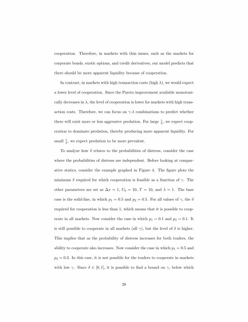
To analyze how δ relates to the probabilities of distress, consider the case

where the probabilities of distress are independent. Before looking at compar-

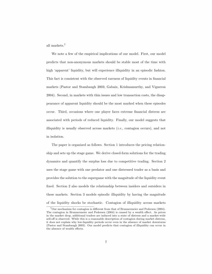
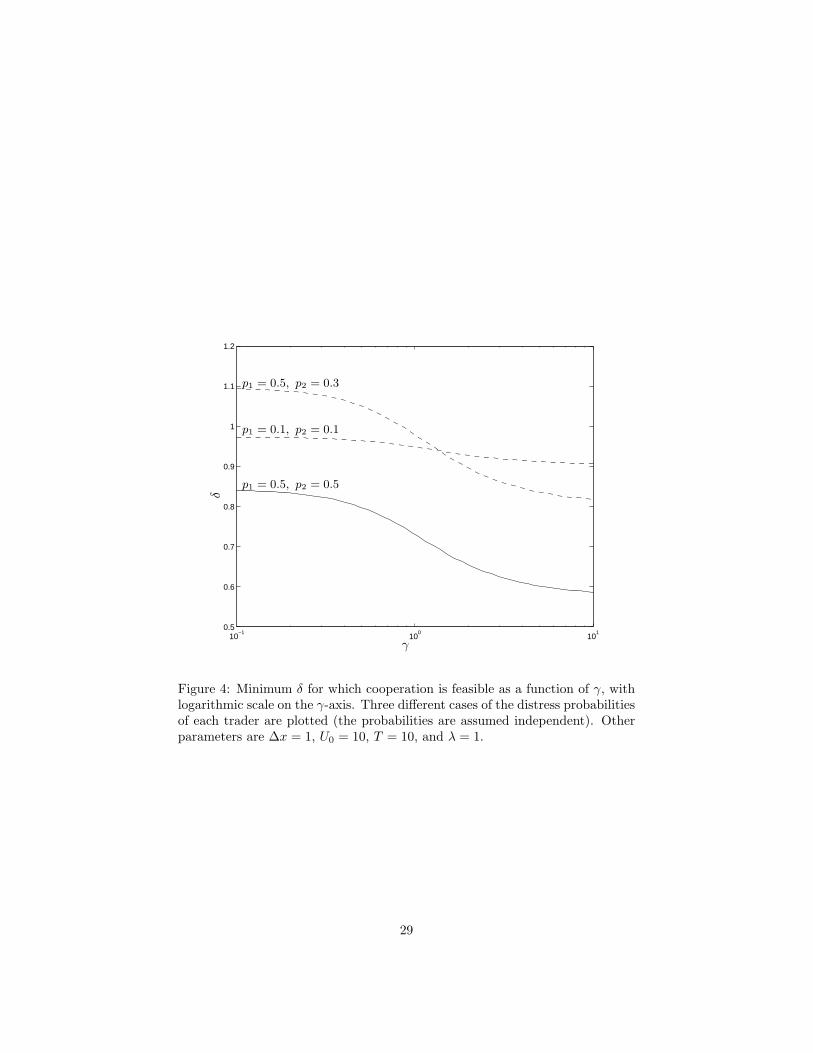
ative statics, consider the example graphed in Figure 4. The figure plots the

minimum δ required for which cooperation is feasible as a function of γ. The

other parameters are set as ∆x = 1, U0 = 10, T = 10, and λ = 1. The base

case is the solid-line, in which p1 = 0.5 and p2 = 0.5. For all values of γ, the δ

required for cooperation is less than 1, which means that it is possible to coop-

erate in all markets. Now consider the case in which p1 = 0.1 and p2 = 0.1. It

is still possible to cooperate in all markets (all γ), but the level of δ is higher.

This implies that as the probability of distress increases for both traders, the

ability to cooperate also increases. Now consider the case in which p1 = 0.5 and

p2 = 0.3. In this case, it is not possible for the traders to cooperate in markets

with low γ. Since δ ∈ [0, 1], it is possible to find a bound on γ, below which

28

10−1

100

101

0.5

0.6

0.7

0.8

0.9

1

1.1

1.2

δ

γ

p1 = 0.5, p2 = 0.5

p1 = 0.1, p2 = 0.1

p1 = 0.5, p2 = 0.3

Figure 4: Minimum δ for which cooperation is feasible as a function of γ, withlogarithmic scale on the γ-axis. Three different cases of the distress probabilitiesof each trader are plotted (the probabilities are assumed independent). Otherparameters are ∆x = 1, U0 = 10, T = 10, and λ = 1.

29

we should not observe cooperation. It is interesting to note that symmetry (in

distress probabilities) between the traders is an important driver of cooperation.

In markets with a low γ, a small decrease in one trader’s distress probability

may be enough to cause the traders to abandon their cooperative relationship.

Without loss of generality, assume δ1 = δmin (that is, p1 < p2). Equa-

tion (18) can be rewritten as

δ1 =Vp

p2 [p1∆V2 − Vp] + p1∆Vd + Vp. (19)

This shows that δ1 is monotonically increasing in p2 (since we can establish that

Vp ≥ ∆V2 from Vp/∆Vd > 1/2 in Result 3 and ∆Vd = ∆V2 + Vp). This means

that a larger probability for trader 2 makes cooperation more difficult (that is,

cooperation is possible only under a narrower range of market conditions). We

can also rewrite Equation (18) as

δ1 =Vp

p1 [(1 − p2)∆Vd + 2p2∆V2 + p2Vp] + (1 − p2)Vp, (20)

which shows that δ1 is monotonic decreasing in p1. This means that a bigger

probability for trader 1 makes cooperation easier (that is, possible under a wider

range of market conditions).

If traders are infinitely patient (δ = 1), and without loss of generality p1 <

p2, to support cooperation it must be that

p1 ≥ p2Vp

∆Vd− p1p2

∆V2

∆Vd. (21)

Evaluating Equation (21) under extreme market conditions provides more in-

sight into the relative values of the distress probabilities which are conducive to

30

cooperation. Taking the limits γ/λ → 0 and γ/λ → ∞, Equation (21) becomes

p1 ≥ 45p2 − 1

5p1p2 and p1 ≥ 1

2p2 − 1

2p1p2. (22)

If distress events are infrequent (p1, p2 1), then the size of the smaller player

relative to larger player is bounded by

p1

p2≥ Vp

∆Vd. (23)

In the limit cases (γ/λ → 0 and γ/λ → ∞) this is

p1

p2≥ 4

5and

p1

p2≥ 1

2. (24)

The traders’ distress probabilities need to be sufficiently symmetric or else co-

operation is not possible. Equation (24) provides the lower bounds on trader

1’s relative distress probabilities in order to sustain cooperation. An important

consequence of this is that if the probability of distress is linked to the market

share of external clients that a trader services, it may benefit a large trader to

allow a smaller trader to grow in size so that a Pareto superior outcome for

the strategic traders can be achieved or maintained. We briefly address this

relationship as follows.

Consider the following scenario in which there exists two strategic traders

and a representative outsider who seeks to trade a block of an asset. The

strategic traders have two alternatives when an outsider needs to trade. They

may initiate a predatory strategy, race and fade the external player to the

market, and earn a profit by affecting the price of the asset. Alternatively, the

outsider may become a client of the traders so that the traders may exact rents

31

for use of their services (these rents may arise in the form of a bid-ask spread).

The fact that there exists a cooperative outcome in this market between the

insiders provides a means by which a relatively stable, albeit widened, bid-ask

spread may exist, and we do not necessarily observe price volatility when a

non-member needs liquidity. The amount of the surplus available between the

traders and the client is ∆Vd, since the outsider is indifferent between receiving

Vd, and paying ∆Vd in order to receive V1 when using the services of the strategic

traders. 18

The external client uses each trader with probabilities p1 and p2. Equa-

tion (21) implies that the relative market shares of the traders should be rea-

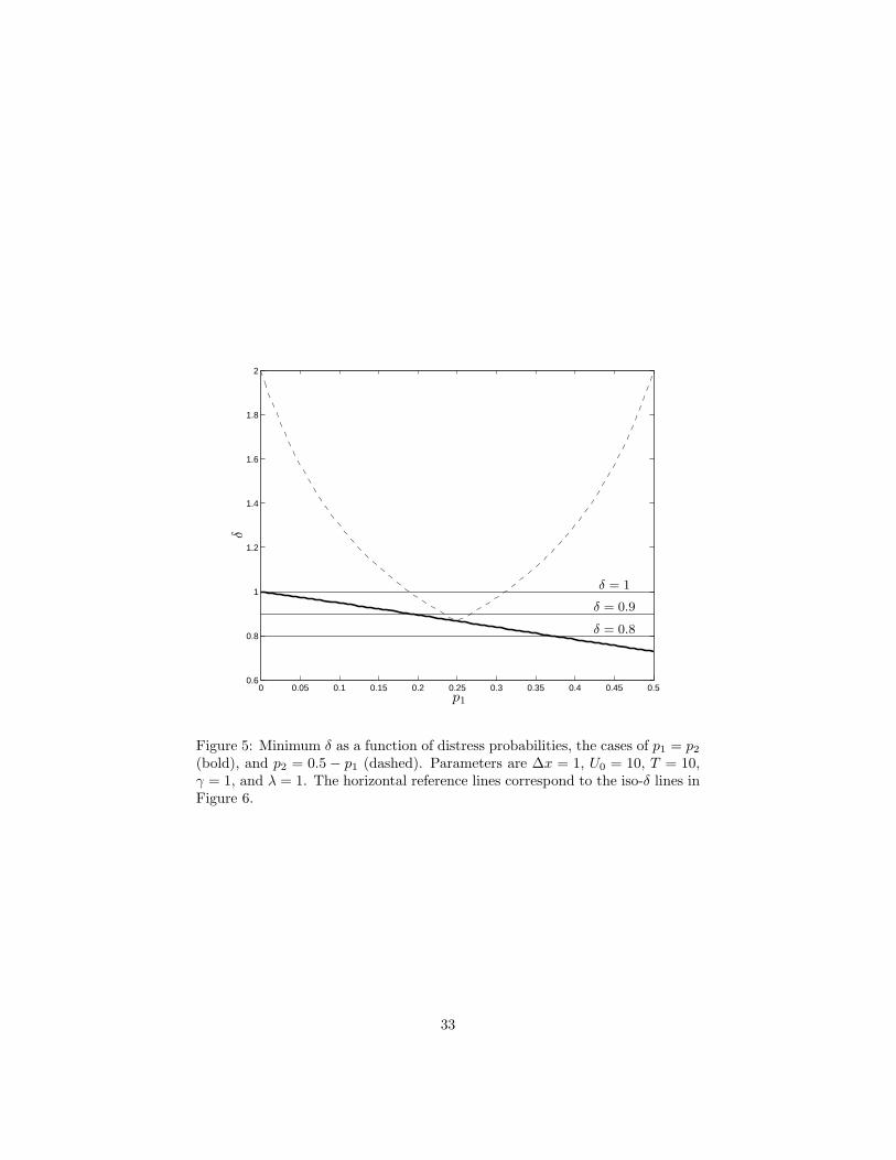
sonably symmetric to support cooperation. Consider the example in Figure 5 in

which the minimum δ necessary to support cooperation is plotted as a function

of p1. Two scenarios are demonstrated: p1 = p2 (bold line) and p1 + p2 = 0.5

(dotted line). When the traders’ distress probabilities (market shares) are sym-

metric, cooperation is always possible, as long as traders are sufficiently patient.

However, when the market shares are asymmetric and p1 < 0.18 (36% market

share) or p1 > 0.32 (64% market share), cooperation is not possible. Therefore,

if one trader has a larger than 64% market share, he may find it beneficial to

allow his opponent to gain market share so that their ongoing Pareto supe-

rior relationship may continue. This finding may explain why deviations in the

bid-ask spread may be observed in practice without resulting in price wars.18To determine the division of this surplus between the insiders and the external player, it is

possible to use a generalized Nash bargaining solution in which the insiders receive fraction τof the surplus and the client receives fraction 1−τ . In the example that we consider (Figure 5),we assume τ = 1, without loss of generality. Relaxing this assumption does does not lead todifferent comparative statics.

32

0 0.05 0.1 0.15 0.2 0.25 0.3 0.35 0.4 0.45 0.50.6

0.8

1

1.2

1.4

1.6

1.8

2

δ

p1

δ = 1

δ = 0.9

δ = 0.8

Figure 5: Minimum δ as a function of distress probabilities, the cases of p1 = p2

(bold), and p2 = 0.5 − p1 (dashed). Parameters are ∆x = 1, U0 = 10, T = 10,γ = 1, and λ = 1. The horizontal reference lines correspond to the iso-δ lines inFigure 6.

33

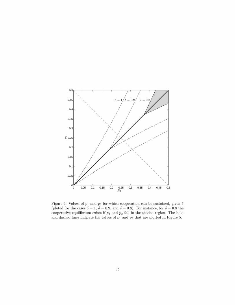
Figure 6 illustrates, for three different values of δ, the (p1, p2) pairs that

support cooperation. The values of δ plotted are 1, 0.9 and 0.8. The other

parameters are ∆x = 1, U0 = 10, T = 10, γ = 1, and λ = 1. The shaded

region corresponds to the (p1, p2) pairs for which cooperation is possible if both

traders use a discount factor δ = 0.8. Note that the boundaries of the sets are

not straight lines due to the bilinear terms p1p2, but are nearly so for small values

of p1 and p2. For δ = 1, and for small probabilities, the set boundaries go to

the origin with slope Vp/∆Vd and ∆Vd/Vp. As the sum of the two probabilities

becomes smaller, traders are required to be of more similar sizes for a cooperative

outcome to be feasible. Note that the bold and dashed lines correspond to the

cases plotted in Figure 5. Considering cases with smaller overall frequency of

events p1 + p2 corresponds to moving the dashed line to the lower-left. Figure 5

and Figure 6, therefore, demonstrate that the traders’ market shares need to be

sufficiently symmetric or else cooperation is not possible.

In the next section, we consider these relationships when the liquidity event

(∆x) is stochastic across time. Also, we evaluate the effect of multi-market

contact and contagion of illiquidity.

3 Episodic Illiquidity and Contagion

3 A Shocks of Random Magnitude and Episodic Illiquidity

In Section 2, we evaluated the requirements for cooperation given that ∆x is a

fixed amount of the asset. In that formulation, if cooperation is possible (based

34

0 0.05 0.1 0.15 0.2 0.25 0.3 0.35 0.4 0.45 0.50

0.05

0.1

0.15

0.2

0.25

0.3

0.35

0.4

0.45

0.5

p1

p2

δ = 1 δ = 0.9 δ = 0.8

Figure 6: Values of p1 and p2 for which cooperation can be sustained, given δ(ploted for the cases δ = 1, δ = 0.9, and δ = 0.8). For instance, for δ = 0.8 thecooperative equilibrium exists if p1 and p2 fall in the shaded region. The boldand dashed lines indicate the values of p1 and p2 that are plotted in Figure 5.

35

on the market parameters and δ), the traders never deviate. To characterize

episodic illiquidity, ∆x is better modeled as a random variable. In the event of

a large ∆x it is more profitable for the traders to deviate for a one-time gain.

However, instead of initiating the grim-trigger strategy outlined in Section 2,

there are more profitable strategies available to the cartel. The approach that

we take is along the lines of Rotemberg and Saloner (1986).

The large traders implicitly agree to restrain from predating when the mag-

nitude of the shock is below some threshold ∆x and, conversely, not to punish

other players in future periods for predating when the shock is above that thresh-

old. That is, when a player has trading requirement that exceeds ∆x, the other

player will predate, but cooperation is resumed in subsequent periods. This

equilibrium behavior results in episodically increased volatility.19

Another way to describe this equilibrium is that each trader agrees to restrain

from predating on the other, but only as long as they behave ‘responsibly’ in

their risk management. This creates a natural restriction on the exposure that

each trader can take without a substantial increase in the risk of their portfolio.

The value of ∆x which is optimal for the cartel (in the sense of leading to

the highest expected value for its members) can be computed for any distri-

bution of the trading requirement for each player. In general, ∆x can only be

characterized implicitly.

Result 5 (Shocks of Random Magnitude) Consider that the trading require-

19Episodic illiquidity also occurs during extreme financial distress. During extreme distress,a member of the oligopoly becomes a finite concern. Because the horizon of this game isfinite, the players work out their strategy profiles by backwards induction and cooperationdisappears.

36

ments for each of two players are random shock magnitudes ∆x that are dis-

tributed i.i.d. according to the density f(y), which we assume to be

(i) symmetric, f(y) = f(−y),

(ii) with unbounded support, f(y) > 0,∀y ∈ R,

(iii) and with finite variance,∫ ∞−∞ y2f(y)dy < ∞.

A strategy with episodic predation with threshold ∆x is feasible with any ∆x that

satisfies

2C

∫ ∆x

0

y2f(y)dy ≥ K∆x2. (25)

The supremum of ∆x such that the inequality is satisfied exists, and we designate

it by ∆x. The following strategy profile constitutes a sub-game perfect Nash

equilibrium. At time t = 0, we predate if |∆x| > ∆x, and otherwise cooperate.

At time t = 0,

1. If the history of play ht−1 is such that for every period in which |∆x| < ∆x

there was no predation, then

(a) If |∆x| > ∆x, predate this period.

(b) If |∆x| < ∆x, cooperate.

2. If ht−1 is such that for |∆x| < ∆x, there was predation, then predate.

The constants above are

C =δ

1 − δ(p10Kd + 2p11K2 − p01K) (26)

37

0 0.5 1 1.5 2 2.5 3 3.5 40

1

2

3

4

5

6

7

8

a b x

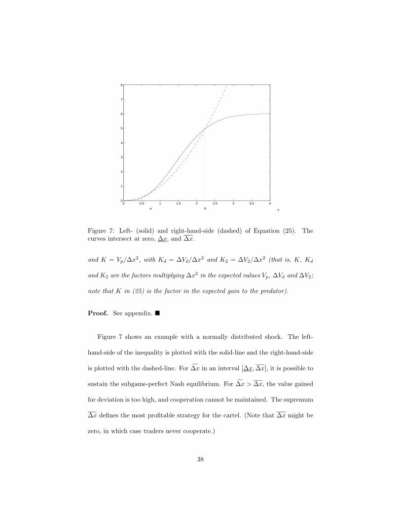
Figure 7: Left- (solid) and right-hand-side (dashed) of Equation (25). Thecurves intersect at zero, ∆x, and ∆x.

and K = Vp/∆x2, with Kd = ∆Vd/∆x2 and K2 = ∆V2/∆x2 (that is, K, Kd

and K2 are the factors multiplying ∆x2 in the expected values Vp, ∆Vd and ∆V2;

note that K in (25) is the factor in the expected gain to the predator).

Proof. See appendix.

Figure 7 shows an example with a normally distributed shock. The left-

hand-side of the inequality is plotted with the solid-line and the right-hand-side

is plotted with the dashed-line. For ∆x in an interval [∆x,∆x], it is possible to

sustain the subgame-perfect Nash equilibrium. For ∆x > ∆x, the value gained

for deviation is too high, and cooperation cannot be maintained. The supremum

∆x defines the most profitable strategy for the cartel. (Note that ∆x might be

zero, in which case traders never cooperate.)

38

The nature of the solutions is essentially independent of the scale parameter

of the distribution. Consider a family of distributions fa(y) = af(ay). If we

consider solutions in terms of ∆x/a, the set of feasible thresholds is independent

of the asset parameters (here C and K). The inequality is equivalent to

2C

K

∫ ∆xa

0

y2fa(y)dy ≥(

∆x

a

)2

, (27)

so that, after the corresponding scaling, the solutions to the inequality are con-

stant with scaling of the distribution.

As an example, consider the zero-mean normal distribution

f(y) =1

σ√

2πe−

12

y2

σ2 . (28)

Rewriting the inequality as

K

C

(∆x

σ

)2

≤ 2∫ ∆x

σ

0

y2 1√2π

e−12 y2

dy, (29)

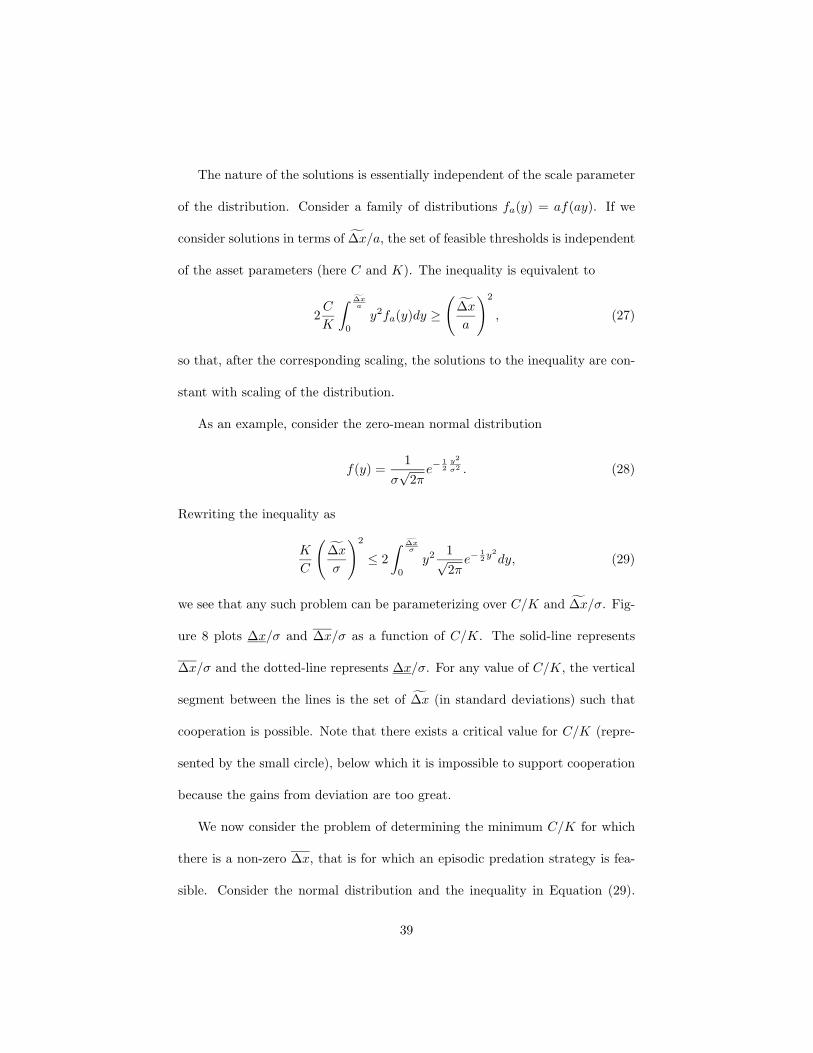
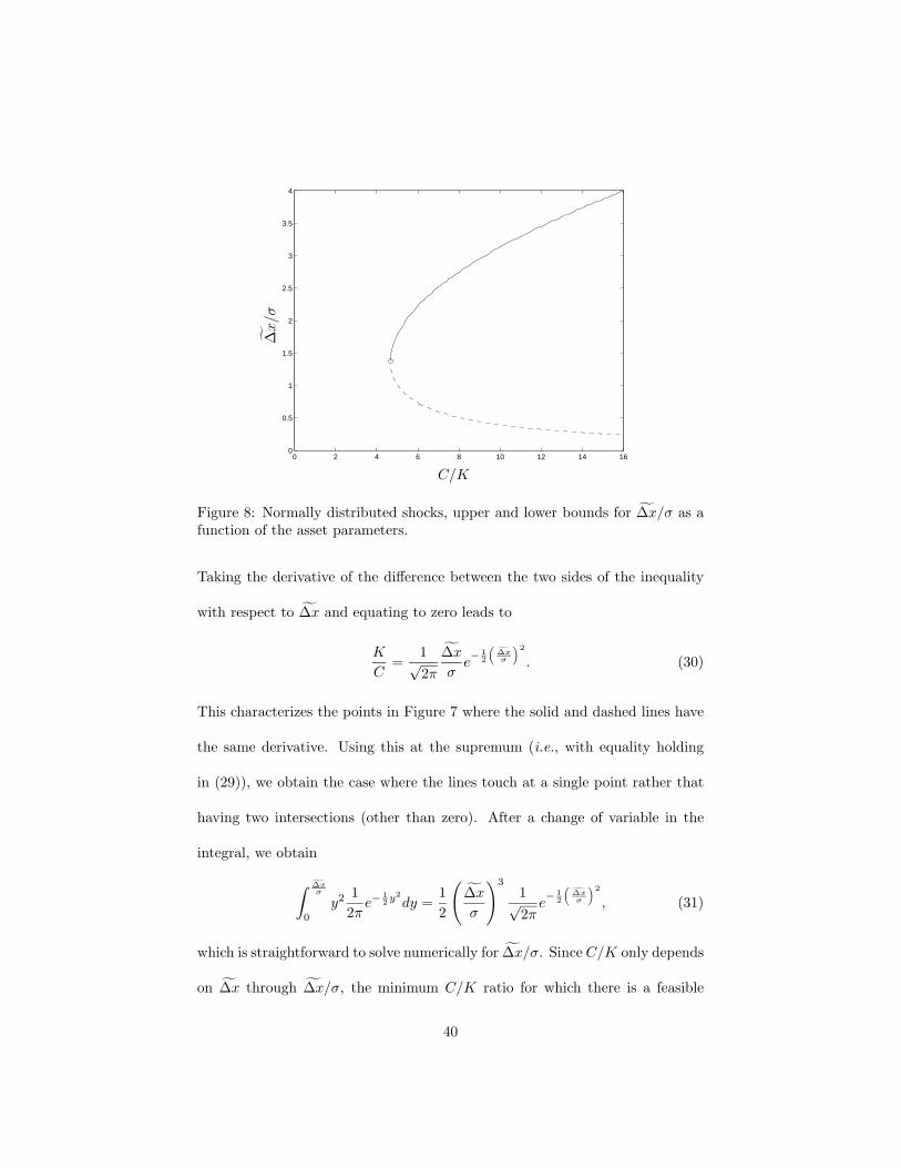
we see that any such problem can be parameterizing over C/K and ∆x/σ. Fig-

ure 8 plots ∆x/σ and ∆x/σ as a function of C/K. The solid-line represents

∆x/σ and the dotted-line represents ∆x/σ. For any value of C/K, the vertical

segment between the lines is the set of ∆x (in standard deviations) such that

cooperation is possible. Note that there exists a critical value for C/K (repre-

sented by the small circle), below which it is impossible to support cooperation

because the gains from deviation are too great.

We now consider the problem of determining the minimum C/K for which

there is a non-zero ∆x, that is for which an episodic predation strategy is fea-

sible. Consider the normal distribution and the inequality in Equation (29).

39

0 2 4 6 8 10 12 14 160

0.5

1

1.5

2

2.5

3

3.5

4

∆x/σ

C/K

Figure 8: Normally distributed shocks, upper and lower bounds for ∆x/σ as afunction of the asset parameters.

Taking the derivative of the difference between the two sides of the inequality

with respect to ∆x and equating to zero leads to

K

C=

1√2π

∆x

σe− 1

2

(∆xσ

)2

. (30)

This characterizes the points in Figure 7 where the solid and dashed lines have

the same derivative. Using this at the supremum (i.e., with equality holding

in (29)), we obtain the case where the lines touch at a single point rather that

having two intersections (other than zero). After a change of variable in the

integral, we obtain

∫ ∆xσ

0

y2 12π

e−12 y2

dy =12

(∆x

σ

)31√2π

e− 1

2

(∆xσ

)2

, (31)

which is straightforward to solve numerically for ∆x/σ. Since C/K only depends

on ∆x through ∆x/σ, the minimum C/K ratio for which there is a feasible

40

strategy of the episodic predation type does not depend on the scale parameter of

the distribution. For the normal distribution, the minimum C/K for which there

is a non-zero ∆x, that is for which an episodic predation strategy is feasible,

is C/K = 4.6729 for any σ. The threshold for this C/K ratio is ∆x = ∆x =

1.3688σ.

3 B Contagion across markets

Suppose that the members of the oligopoly can cooperate in more than one

market. For example, consider institutional traders who dominate mortgage

markets are also strategic traders in other fixed income markets. If a liquidity

event is large enough to disturb cooperation in one market, it may also affect

cooperation in the others. According to Bernheim and Whinston (1990), if

markets are not identical, multimarket contact supports cooperation. In our

case, and since most assets are not perfectly correlated, multi-market contact

makes it easier to maintain cooperation. In this section, we demonstrate the

effects of multi-market contact on the episodic illiquidity that occurs across

markets.

Consider that the traders participate in n markets, where the trading re-

quirement in each market is a stochastic random variable. We define a liquidity

event to be such that all trading targets for each of the n assets have the same

sign (i.e., liquidity shocks occur in the same direction in all markets). The trad-

ing targets are modeled as jointly normal and conditionally independent given

that they are either all positive or all negative. We also use the simplifying

41

assumption that trading targets in all the assets have the same variance. The

density in the positive orthant (y such that yi ≥ 0, all i) and in the negative

orthants (y such that yi ≤ 0, all i) is

f(y) =2n−1

σn(2π)n/2e−

yT y

σ2 , (32)

and zero elsewhere.

The shape of the optimal region for cooperation is spherical. This is the

region in which the temptation to predate, which is proportional to∑n

i=1 ∆x2i ,

is constant.

The inequality for n assets involves an integral in n dimension which, using

the radial symmetry of the normal distribution can be written as

2C

∫ r

0

Snyn+1f(y)dy ≥ Kr2, (33)

where r is the radius of the cooperation region, and

Sn =12n

2πn2

Γ(n2 )

(34)

is the area of the intersection of the sphere of unit radius in n dimension with

the positive orthant. It can easily be verified that, as for the one-asset case, the

nature of the solutions is essentially independent of the scale parameter of the

distribution (the standard deviation).

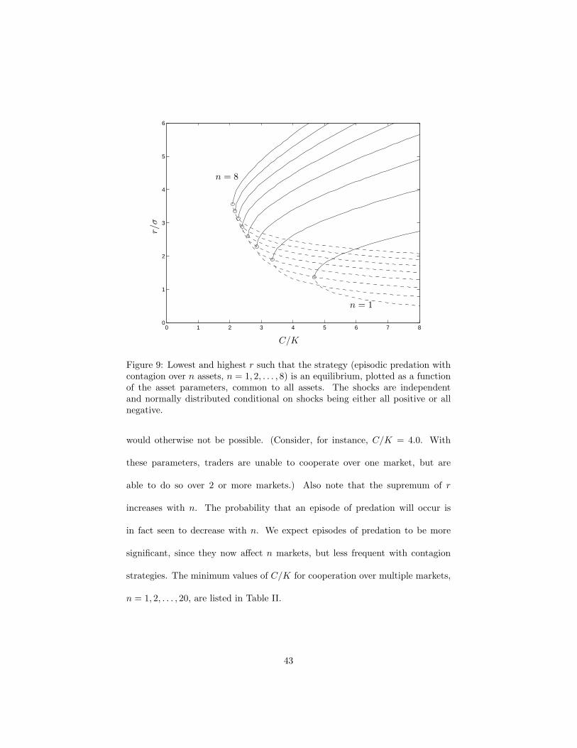
Figure 9 is the multi-market version of Figure 8 in that it plots ∆x and

∆x for episodic illiquidity over n markets, n = 1, 2, . . . , 8. The minimum value

of C/K that is required to support cooperation decreases as the number of

markets increases. Adding markets can make cooperation possible where it

42

0 1 2 3 4 5 6 7 80

1

2

3

4

5

6

r/σ

C/K

n = 1

n = 8

Figure 9: Lowest and highest r such that the strategy (episodic predation withcontagion over n assets, n = 1, 2, . . . , 8) is an equilibrium, plotted as a functionof the asset parameters, common to all assets. The shocks are independentand normally distributed conditional on shocks being either all positive or allnegative.

would otherwise not be possible. (Consider, for instance, C/K = 4.0. With

these parameters, traders are unable to cooperate over one market, but are

able to do so over 2 or more markets.) Also note that the supremum of r

increases with n. The probability that an episode of predation will occur is

in fact seen to decrease with n. We expect episodes of predation to be more

significant, since they now affect n markets, but less frequent with contagion

strategies. The minimum values of C/K for cooperation over multiple markets,

n = 1, 2, . . . , 20, are listed in Table II.

43

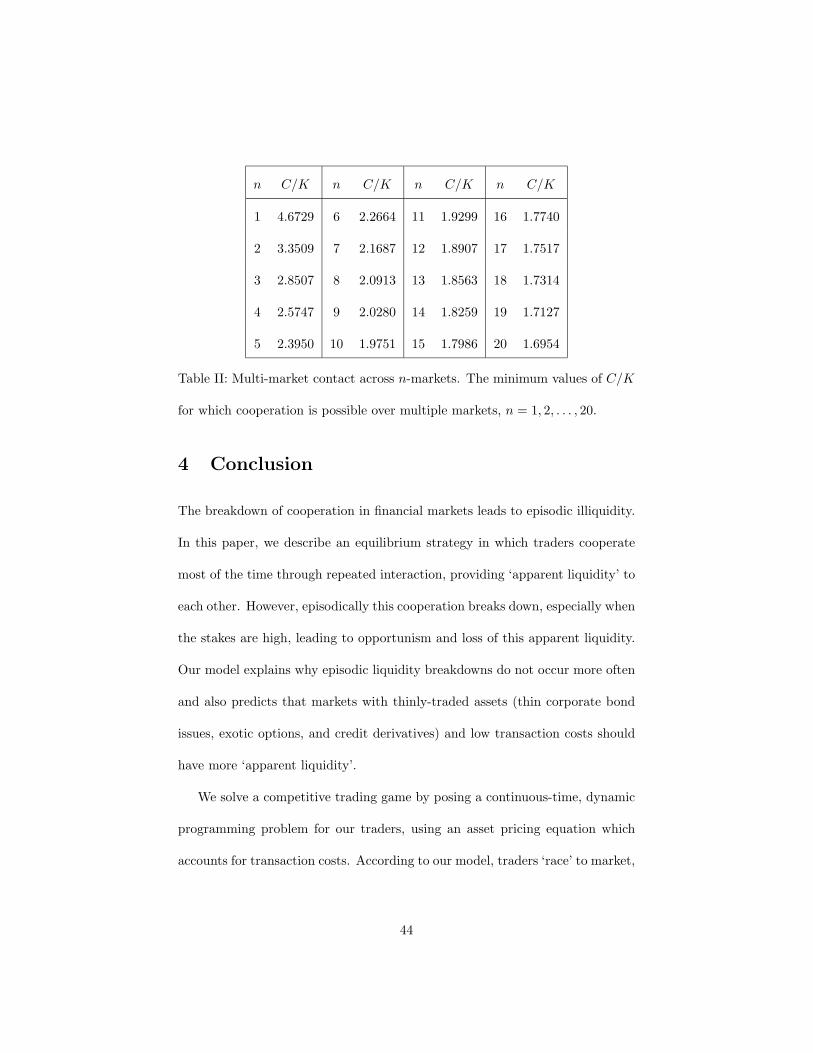
n C/K n C/K n C/K n C/K

1 4.6729 6 2.2664 11 1.9299 16 1.7740

2 3.3509 7 2.1687 12 1.8907 17 1.7517

3 2.8507 8 2.0913 13 1.8563 18 1.7314

4 2.5747 9 2.0280 14 1.8259 19 1.7127

5 2.3950 10 1.9751 15 1.7986 20 1.6954

Table II: Multi-market contact across n-markets. The minimum values of C/K

for which cooperation is possible over multiple markets, n = 1, 2, . . . , 20.

4 Conclusion

The breakdown of cooperation in financial markets leads to episodic illiquidity.

In this paper, we describe an equilibrium strategy in which traders cooperate

most of the time through repeated interaction, providing ‘apparent liquidity’ to

each other. However, episodically this cooperation breaks down, especially when

the stakes are high, leading to opportunism and loss of this apparent liquidity.

Our model explains why episodic liquidity breakdowns do not occur more often

and also predicts that markets with thinly-traded assets (thin corporate bond

issues, exotic options, and credit derivatives) and low transaction costs should

have more ‘apparent liquidity’.

We solve a competitive trading game by posing a continuous-time, dynamic

programming problem for our traders, using an asset pricing equation which

accounts for transaction costs. According to our model, traders ‘race’ to market,

44

selling quickly in the beginning of the period. In the equilibrium strategy traders

sell-off at a decreasing exponential rate. Also in equilibrium, predators initially

race distressed traders to market, but eventually ‘fade’ them and buy back. The

presence of predators in the market leads to a surplus loss to liquidity providers

in the market.

We then model cooperation in the market by embedding this predatory

stage game in a dynamic game with infinite horizon. Cooperation allows for

the trading of large blocks of the asset at more favorable prices. We show how

traders can cooperate to avoid the surplus loss due to predatory trading and

provide predictions as to what magnitude of liquidity event is required to trigger

an observable shock in the market. Further, we make predictions on how market

depth and transaction costs will affect the ability to cooperate.

In conclusion, we believe our work presents a strong argument for the level of

predation or cooperation in financial markets being a determinant of the amount

of liquidity available, and a factor causing the episodic nature of illiquidity.

45

A Derivations

Proof of Result 1 (General Solution)

Given that each player’s objective is linear in Ut, and that the strategies are

open-loop, we can bring the expectation inside the integral and consider the

equivalent problem with a deterministic asset pricing equation, in which Ut is

replaced by a constant u = U0,

Pt = u + γ

n∑j=1

Xjt + λ

n∑j=1

Y jt . (35)

With the multiplier function Zit associated with the constraint dXi

t = Y it dt,

necessary optimality conditions for the problem faced by trader i are

u + γ∑n

j=1 Xjt + λ

∑nj=1 Y j

t + λ Y it + Zi

t = 0

dZit = −γ Y i

t dt.

(36)

Differentiating the first equation with respect to t, and substituting the second,

γn∑

j=1

Y jt dt + λ

n∑j=1

dY jt + λdY i

t − γY it dt = 0. (37)

The n such equations for each trader can be collected together as

λ(I + 11T )dYt = γ(I − 11T )Ytdt, (38)

where I is the n × n identity matrix, 1 is the n-vector with all entries equal

to one, and 11T is an n × n matrix with all elements equal to one. From the

formula for the inverse of the rank-one update of a matrix, the inverse of I+11T

is I − 1n+111T , which we use to write the linear dynamic system in the form

dYt =γ

λAYtdt, where A = I − 2

n + 111T . (39)

46

Since A1 = 1 − 2n+1n1 = −n−1

n+1 1, the vector of ones is an eigenvector of the

matrix A, with associated eigenvalue −n−1n+1 . Likewise, vectors in the null-space

of 1 are eigenvectors of A, with eigenvalue 1: for v orthogonal to the vector of

ones, that is satisfying 1T v = 0, we find that Av = v. The dimension of this

sub-space, and multiplicity of the eigenvalue 1, is n − 1. Since the matrix A

has a full set of n independent eigenvectors, all Jordan blocks are of size 1 and

solutions to the system of linear differential equations are as stated in (4). This

characterizes any continuous policy (with continuous dual functional) which is

an extremal of the problem. Since a (unique) continuous extremal exists, from

problem convexity it is the only extremal of the problem. The n trading target

constraints and 1T b = 0 uniquely determine the n free parameters in the solution

(integrate the Y it , equate to ∆xi, and solve for a and b).

Convexity ensures that any solution is identical almost everywhere to the one

given in this result (i.e., has the same integrals). Further restrictions can be

imposed on the Yt if desired, such as being of bounded variation. Alternatively,

smoothness can be ensured by defining the solution to the continuous-time prob-

lem as the limit of the solutions to a sequence of discrete-time problems, which

is the approach we will use to analyze the closed-loop version of this problem in

Appendix B.

We next show a Lemma and Corollary, which will be of use in proving Result 2.

Lemma: The function f : R+ → R

f(y) =1 + e−y

1 − e−y− 2

y(40)

47

is positive increasing.

Proof: We first show limy→0 f(y) = 0. Applying l’Hopital’s rule, we find

limy→0

f(y) = limy→0

−ye−y + 1 + e−y − 2e−y

1 − e−y + ye−y= lim

y→0

ye−y

2e−y − ye−y= 0. (41)

We now show f ′(y) > 0.

f ′(y) =−2e−y

(1 − e−y)2+

2y2

=2

(1 − e−y)2y2

(−y2e−y + 1 + e−2y − 2e−y). (42)

For y > 0, the denominator is positive. We show that the numerator is also

positive, g(y) = −y2e−y + 1 + e−2y − 2e−y > 0, from g(0) = 0 and g′(y) > 0:

g′(y) = −2ye−y + y2e−y − 2e−2y + 2e−y = e−y(−2y + y2 − 2e−y + 2

). (43)

Likewise, we show h(y) = −2y+y2−2e−y +2 > 0, from h(0) = 0 and h′(y) > 0:

h′(y) = −2 + 2y + 2e−y, (44)

which is positive if e−y > 1− y, which is true for any y = 0 (from the intercept

and derivative at zero and from the convexity of the exponential).

Corollary: The function f : R+ → R

f(y) = y1 + e−y

1 − e−y(45)

is positive increasing.

Proof: Write

f(y) = yf(y) + 2, (46)

where f is as in the previous Lemma. The product of two positive increasing

functions is positive increasing.

48

Proof of Result 2 (Expected Total Surplus and Loss for Multiple

Traders)

The expected surplus is obtained by integration of

−Pt

n∑i=1

Y it = −Pt na e−

n−1n+1

γλ t (47)

over t ∈ [0, T ], followed by algebraic simplification. The proofs of the mono-

tonicities are direct applications of the Lemma above or of its Corollary, using

y = T , y = γ, y = 1λ , and y = n−1

n+1 (with n relaxed to be in R). For λ and

n, we also need the fact that the composition of two monotonic functions is

monotonic.

Proof of Result 3 (Expected Total Surplus and Loss for Two Traders)

By Equation (7), Y = Y dt + Y p

t = 2ae−13

γλ t. By integration of −PtY over t ∈

[0, T ], followed by algebraic simplification, the results in Equations (12) and (15)

are derived. The monotonicities are verified by differentiation of Equation (15).

We define V− = Vd − Vp and Y− = Y dt − Y p

t = 2beγλ t. Integrate −PtY− over

t ∈ [0, T ] and simplify to obtain

V− = Vd − Vp = − u ∆x − γeΓ

eΓ − 1∆x2. (48)

Vd and Vp are obtained by simplification of (V2 + V−)/2 and (V2 − V−)/2.

The proof for the monotonicity of Vp

∆Vdis along the same lines as for Result 2

(with lengthier algebra). The bounds on Vp

∆Vdare the limits at 0 and +∞,

obtained by applying l’Hopital’s rule as needed.

Proof of Result 4 (Repeated Game with Two Symmetric Traders)

For trader 1, the gains from cooperation must exceed those of one-time deviation

49

and infinite non-cooperation or

δ1

1 − δ1[p10V1(∆x)+

12p11V1(2∆x)] ≥ Vp +

δ1

1 − δ1[p01Vp +p10Vd +

12p11V2(2∆x)].

(49)

Since ∆V2 = V1−V2 is quadratic in ∆x, we have that 12 ∆V2(2∆x) = 2∆V2(∆x)

(we then omit the argument when it is ∆x). The first equation in (18) follows

by solving for δ1. The second equation is derived similarly for trader 2. For

both traders to cooperate, it must be that δ ≥ maxδ1, δ2. The monotonicities

can be proved algebraically, along the same lines as for Result 2.

Proof of Result 5 (Shocks of Random Magnitude)

Equation (49) can be written in this context as Equation (25), where f is the

density of ∆x and C and K are as defined. For values of C sufficiently large or

values of K sufficiently small, Equation (25) will be satisfied and there will exist

a ∆x such that cooperation is possible. As long as |∆x| < ∆x, the traders will

cooperate since the value of cooperating exceeds that of a one-time deviation

and subsequent grim-trigger play. If |∆x| ≥ ∆x, the traders will predate and

resume cooperation in the next period if possible. If Equation 25 is not satisfied,

then cooperation is not possible and the traders will always predate. Thus, there

exists a subgame perfect Nash equilibrium as described. The left-hand side of

Equation 25 is bounded since f has finite variance and the right-hand-side is

unbounded. Hence the supremum of ∆x is bounded. For existence of ∆x, note

that zero is a solution.

50

B Closed-loop equilibrium

In our analysis of the stage game, the strategies considered are deterministic.

They are open-loop, in the sense that traders choose their strategies at time

t = 0. It is assumed that traders would not respond to other traders’ deviations

from their optimal strategies. We would have obtained the same solution had

we defined the Y it to be Ft-adapted (where Ft is the filtration of the σ-algebras

generated by Bt). Note however that this is in the strict sense that traders are

aware of the underlying process Ut that defines price fundamentals, but not of

the actual price Pt and of the other players’ trading rates Yt. (The argument

for the solution to this variation on the open-loop problem to be the same as in

Result 1 is based on the value functions’ linearity in Ut, as is done below in this

section.)

We now consider closed-loop strategies, in that traders know or can infer the

other traders’ rate of trading, and respond accordingly. Under such strategies,

Y it is adapted to all the information existing at time t, and players can revise

their trading decisions at any time based on such information. This means

that earlier decisions must account for other players’ response function at later

times. This innability to commit ahead of time to not deviate from a given

strategy over the entire [0, T ] period leads to more aggressive strategies than in

the open-loop case, including faster racing.

Closed-loop strategies are substantially more difficult to analyze than open-

loop, and we do not provide a closed-form solution. We do provide a description

of the equilibrium optimal strategies in terms of a value function with two scalar

51

parameter which satisfy a triangular system of nonlinear differential equations.

Our numerical simulations have shown the open- and closed-loop solutions not

to be substantially different. We provide some analytical justification for this

observation. In particular, from a fixed-point analysis of the Riccati equations,

we provide closed-form expressions for the expected value for each of the players

when T is large.

We derive the closed-loop result for the deterministic case and then show

that it holds for the stochastic pricing equation. We consider strategies where

the trading rate is constant over time increments of length ∆t. The reward for

trader i over each time increment is

ri(u, y,∆t) =∫ ∆t

0

− (u + γ 1Ty τ + λ1Ty

)yidτ (50)

= −(u +

(γ

2∆t + λ

)1Ty

)yi∆t. (51)

We formulate the problem as a dynamic game, with an n+1-dimensional state,

composed of u(t) ∈ R and φ(t) ∈ Rn. The first component, u(t), is the expected

price at time t, including the permanent price impact of previous trades (in

previous notation, u(t) = Ut + γ∑n

i=1 Xit). The n components of φ(t) are the

remaing trading targets for each trader, that is, the amount they still need to

trade by T (in previous notation, φi(t) = xTi − Xit). The state transition over

a period of length ∆t with each player trading at a constant rate yi is

u′(u, y, ∆t) = u + γ 1Ty ∆t, (52)

φ′(φ, y,∆t) = φ − y∆t. (53)

52

The value functions for each of the n traders must simultaneously satisfy

V i(u, φ, t) = maxyi

ri(u, y, ∆t) + V i(u′(u, y, ∆t), φ′(φ, y,∆t), t + ∆t),

i = 1, . . . , n. (54)

We will show that the value functions can be represented in the form

V i(u, φ, t) = −uφi − α(t)φi1Tφ + β(t)(1Tφ

)2, (55)

and derive Riccati equations for α(t), β(t) ∈ R. We take the limit ∆t → 0 to

find the differential equations for the continuous-time case.

Substituting (55), (51), (52), and (53) in (54) and letting ∆t → 0, we obtain

−dα(t)dt

φi1Tφ +dβ(t)

dt

(1Tφ

)2=

= maxyi

−λ yi1Ty − γ φi1Ty + α φi1Ty + α yi1Tφ − 2β 1Ty 1Tφ. (56)

Differentiating with respect to yi and equating to zero, we obtain the optimality

condition

λ(yi + 1Ty) = (α − γ)φi + (α − 2β)1Tφ, (57)

which we collect over i = 1, . . . , n as

λ(I + 11T )y =((α − γ)I + (α − 2β)11T

)φ. (58)

Multiplying on the left by 1λ (I − 1

n+111T ), we solve for the equilibrium trading

rates as a function of the state,

y =1λ

((α − γ)I +

1n + 1

(−2β + γ)11T

)φ, (59)

which can equivalently be written individually as

yi =1λ

((α − γ)φi +

1n + 1

(−2β + γ)1Tφ

), i = 1, . . . , n. (60)

53

The sum of the trading rates is found to be

1Ty =1λ

(α − 2

n

n + 1β − 1

n + 1γ

)1Tφ. (61)

Substituting (60) and (61) in (56), we verify that the structure of the value

function as postulated in (55) is in fact preserved over time (more strongly, it

can be verified that the structure is preserved before letting ∆t → 0). Collecting

terms and simplifying, we obtain the following triangular representation for the

Riccati equations,

dα

dt=

1λ

α(α − γ), (62)

dβ

dt=

1λ

(2αβ − 1

(n + 1)2(2nβ + γ)2

). (63)

So far we have assumed a deterministic u. The objectives for the determin-

istic case are linear in u, the corresponding optimal policies do not depend on u,

and the value functions were found to be linear in u. Using these value functions

for the stochastic case, the ∂2V i/∂u2 terms in the HJB equations are zero, and

all other terms are as in the HJB equations for the deterministic case. That is,

if given value functions and optimal policies satisfy the HJB equations for the

deterministic case, they also satisfy the HJB equations for the stochastic case.

While the system of nonlinear equations (62) and (63) is difficult to solve in

closed form, a number of its properties can be studied. As T → ∞, and since

the expected values are bounded due to the overall convexity of the problem

and the triangular structure precludes oscillatory behavior, α(0) and β(0) must

converge to fixed points of the differential equations. The fixed points for the

first equation are 0 and γ, of which only α = γ is stable (note that (62) is

54

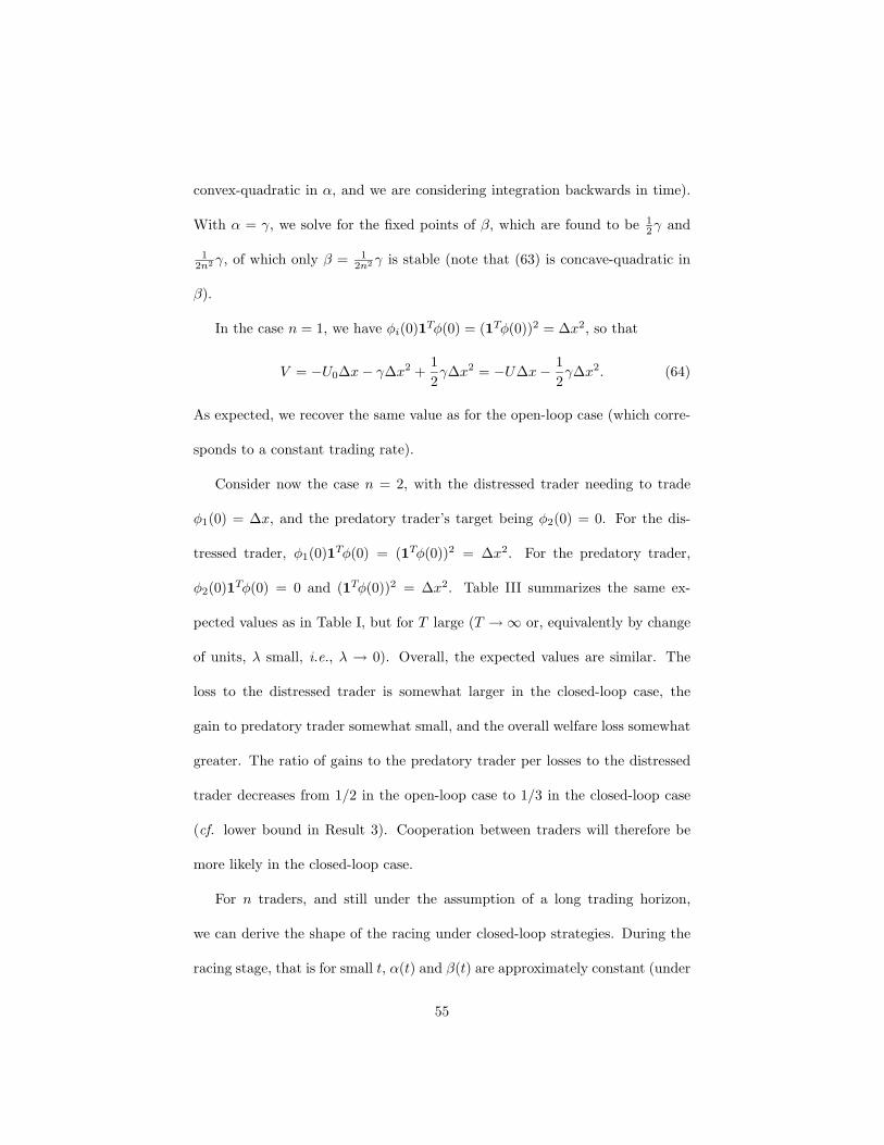
convex-quadratic in α, and we are considering integration backwards in time).

With α = γ, we solve for the fixed points of β, which are found to be 12γ and

12n2 γ, of which only β = 1

2n2 γ is stable (note that (63) is concave-quadratic in

β).

In the case n = 1, we have φi(0)1Tφ(0) = (1Tφ(0))2 = ∆x2, so that

V = −U0∆x − γ∆x2 +12γ∆x2 = −U∆x − 1

2γ∆x2. (64)

As expected, we recover the same value as for the open-loop case (which corre-

sponds to a constant trading rate).

Consider now the case n = 2, with the distressed trader needing to trade

φ1(0) = ∆x, and the predatory trader’s target being φ2(0) = 0. For the dis-

tressed trader, φ1(0)1Tφ(0) = (1Tφ(0))2 = ∆x2. For the predatory trader,

φ2(0)1Tφ(0) = 0 and (1Tφ(0))2 = ∆x2. Table III summarizes the same ex-

pected values as in Table I, but for T large (T → ∞ or, equivalently by change

of units, λ small, i.e., λ → 0). Overall, the expected values are similar. The

loss to the distressed trader is somewhat larger in the closed-loop case, the

gain to predatory trader somewhat small, and the overall welfare loss somewhat

greater. The ratio of gains to the predatory trader per losses to the distressed

trader decreases from 1/2 in the open-loop case to 1/3 in the closed-loop case

(cf. lower bound in Result 3). Cooperation between traders will therefore be

more likely in the closed-loop case.

For n traders, and still under the assumption of a long trading horizon,

we can derive the shape of the racing under closed-loop strategies. During the

racing stage, that is for small t, α(t) and β(t) are approximately constant (under

55

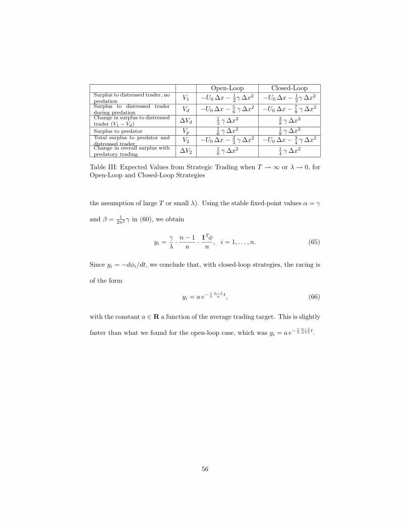
Open-Loop Closed-LoopSurplus to distressed trader, nopredation

V1 −U0 ∆x − 12γ ∆x2 −U0 ∆x − 1

2γ ∆x2

Surplus to distressed traderduring predation

Vd −U0 ∆x − 56 γ ∆x2 −U0 ∆x − 7

8 γ ∆x2

Change in surplus to distressedtrader (V1 − Vd)

∆Vd13 γ ∆x2 3

8 γ ∆x2

Surplus to predator Vp16 γ ∆x2 1

8 γ ∆x2

Total surplus to predator anddistressed trader

V2 −U0 ∆x − 23 γ ∆x2 −U0 ∆x − 3

4 γ ∆x2

Change in overall surplus withpredatory trading

∆V216 γ ∆x2 1

4 γ ∆x2

Table III: Expected Values from Strategic Trading when T → ∞ or λ → 0, forOpen-Loop and Closed-Loop Strategies

the assumption of large T or small λ). Using the stable fixed-point values α = γ

and β = 12n2 γ in (60), we obtain

yi =γ

λ· n − 1

n· 1Tφ

n, i = 1, . . . , n. (65)

Since yi = −dφi/dt, we conclude that, with closed-loop strategies, the racing is

of the form

yi = a e−γλ

n−1n t, (66)

with the constant a ∈ R a function of the average trading target. This is slightly

faster than what we found for the open-loop case, which was yi = a e−γλ

n−1n+1 t.

56

References

Abreu, D. (1988). On the theory of infinitely repeated games with discounting.

Econometrica 56 (2), 383–396.

Abreu, D., D. Pearce, and E. Stacchetti (1986). Optimal cartel equilibria with im-

perfect monitoring. Journal of Economic Theory 39, 251–269.

Acharya, V. and L. Pedersen (2005). Asset pricing with liquidity risk. Journal of

Financial Economics, forthcoming.

Almgren, R. and N. Chriss (1999). Value under liquidation. Risk 12, 61–63.

Almgren, R. and N. Chriss (2000). Optimal execution of portfolio transactions.

Journal of Risk 3, 5–39.

Attari, M., A. Mello, and M. Ruckes (2004). Arbitraging arbitrageurs. Forthcoming

Journal of Finance.

Basar, T. and G. Olsder (1999). Dynamic Noncooperative Game Theory. Philadel-

phia: Society for Industrial and Applied Mathematics.

Battalio, R., A. Ellul, and R. Jennings (2004). Reputation effects in trading on

the new york stock exchange. University of Notre Dame and Indiana Univer-

sity,unpublished.

Berhardt, D., V. Dvoracek, E. Hughson, and I. Werner (2004). Why do larger

orders receive discounts on the london stock exchange? Ohio State University,

unpublished.

Bernheim, B. and M. Whinston (1990). Multimarket contact and collusive behavior.

RAND Journal of Economics 21 (1), 1–26.

Bertsimas, D. and A. Lo (1998). Optimal control of execution costs. Journal of

Financial Markets 1, 1–50.

Brunnermeier, M. and L. Pedersen (2004). Predatory trading. Forthcoming Journal

57

of Finance.

Chan, L. and J. Lakonishok (1995). The behavior of stock prices around institutional

trades. Journal of Finance 50 (4), 1147–1174.

Cocco, J., F. Gomes, and N. Martins (2003). Lending relationships in the interbank

market. London School of Business, unpublished.

DeMarzo, P. and B. Urosevic (2000). Optimal trading by a large shareholder. Stan-

ford Graduate School of Business and Haas School of Business, unpublished.

Desgranges, G. and T. Foucault (2002). Reputation-based pricing and price im-

provements in dealership markets. Universite de Cergy, unpublished.

Dutta, P. and A. Madhavan (1997). Competition and collusion in dealer markets.

Journal of Finance 52 (1), 245–276.

Fedyk, Y. (2001). Large investor optimization problem with direct eect of trades on

prices. Olin School of Business, unpublished.

Foster, F. and S. Viswanathan (1996). Strategic trading when agents forecast the

forecasts of others. Journal of Finance 51 (4), 1437–1478.

Gabaix, X., A. Krishnamurthy, and O. Vigneron (2004). Limits of arbitrage: Theory

and evidence from the mortgage-backed securities market. MIT, unpublished.

Gennotte, G. and A. Kyle (1991). Intertemporal insider trading with a smooth order

flow. Haas School of Business Administration, Berkeley, unpublished.

Green, E. and R. Porter (1984). Noncooperative collusion under imperfect price

information. Econometrica 52 (1), 87–100.

Hansch, O., N. Naik, and S. Viswanathan (1999). Preferencing, internalization, best

execution, and dealer profits. Journal of Finance 54 (5), 1799–1828.

Holthausen, R., R. Leftwich, and D. Mayers (1990). Large block transactions, the

speed of response, and temporary and permanent stock-price effects. Journal of

Financial Economics 26 (1), 71–95.

58

Huberman, G. and W. Stanzl (2000). Optimal liquidity trading. Columbia Univer-

sity and Yale University,unpublished.

Kaul, A., V. Mehrotra, and R. Morck (2000). Demand curves for stocks do

slope down: New evidence from an index weights adjustment. Journal of Fi-

nance 55 (2), 893–912.

Keim, D. and A. Madhavan (1996). The upstairs market for large-block transactions:

Analysis and measurement of price effects. Review of Financial Studies 9 (1), 1–

36.

Massa, M. and A. Simonov (2003). Reputation and interdealer trading: A mi-

crostructure analysis of the treasury bond market. Journal of Financial Mar-

kets 6 (6), 99–141.

Pastor, L. and R. Stambaugh (2003). Liquidity risk and expected stock returns.

Journal of Political Economy 3, 642–685.

Pritsker, M. (2004). Large investors: Implications for equilibrium asset returns,

shock absorption, and liquidity. Federal Reserve, unpublished.

Ramadorai, T. (2003). Persistence, performance, and prices in foreign exchange

markets. Harvard University, unpublished.

Reiss, P. and I. Werner (2003). Anonymity, adverse selection and the sorting of

interdealer trades. Ohio State University, unpublished.

Rotemberg, J. and G. Saloner (1986). A supergame-theoretic model of price wars

during booms. American Economic Review 76 (3), 390–407.

Sadka, R. (2005). Momentum and post-earnings-announcement drift anomalies: The

role of liquidity risk. Journal of Financial Economics, forthcoming.

Seppi, D. (1990). Equilibrium block trading. Journal of Finance 45, 73–94.

Vayanos, D. (1998). Transaction costs and asset prices: A dynamic equilibrium

model. Review of Financial Studies 11 (1), 1–58.

59