eqs 6.1 for windows - mvsoft
TRANSCRIPT

EQS 6.1 for Windows User’s Guide
Peter M. Bentler
Eric J. C. Wu
Multivariate Software, Inc. 15720 Ventura Blvd, Suite 306 Encino, CA 91436-2989 U.S.A.
Tel: (818) 906-0740 • Fax: (818) 906-8205
E-mail: [email protected] • Web: www.mvsoft.com

ii — EQS 6 for Windows
The correct bibliographic citation for this document is as follows:
Bentler, P. M. & Wu, E. J. C. (2002). EQS 6 for Windows User’s Guide.
Encino, CA: Multivariate Software, Inc.
ISBN 1-885898-04-5
Copyright © Peter M. Bentler and Eric J. C. Wu Program Copyright © 1985-2008 Peter M. Bentler
User Interface Copyright © 1992-2008 Eric J. C. Wu
All Rights Reserved Worldwide
Version 6.1, 2008
Printed in the United States of America
BMDP is a trademark of SPSS, Inc. SPSS is a trademark of SPSS, Inc.
SAS is a trademark of SAS Institute, Inc. Lotus 1-2-3 is a trademark of Lotus, Inc.
LISREL is a trademark of Karl Jöreskog and Dag Sörbom.

EQS 6 for Windows — iii
TABLE OF CONTENTS
TABLE OF CONTENTS III
Preface xiv
1. INTRODUCTION 1 Features of the GUI Interface 2
Data Entry and Manipulation 2 Data Imputation 2 Data Exploration 3 Data Presentation 3 Draw a Diagram and Automatic EQS Model Construction 3
Hardware and Software Requirements 4 Installation Procedure 4
Download file installation option: 4 CD installation option: 4
Uninstall EQS 6 for Windows 7 Contents of EQS 6 for Windows Files 8
EQS61.EXE, WINEQS.EXE, and EQS.EXE Files 8 Converting EQS 5 ESS files to EQS 6 ESS Files 8
Where to Go from Here 9
2. A QUICK START TO EQS 6 FOR WINDOWS 10 Step 1: Run EQS 6 for Windows 10 Step 2: Prepare your data 11
Create a Variance/Covariance Matrix 11 Create a New Raw Data File 14 Import an EQS 5 System File 14 Import an SPSS System File 15 Import an ASCII Data File 15
Format 16 Step 3: Activate a Program Function 18
Plotting a Histogram 18 Printing a Plot 19 Summary 20 Discarding Windows and Files 20
A Multiple Regression Analysis 20 Step 4: Create and Run an EQS Model 23
A Path Analysis Model 23 Build a Path Model 23 Run the Path Model 25
A Confirmatory Factor Analytic Model 27

iv — EQS 6 for Windows
1. Building an EQS Model Using the Diagrammer 27 Build EQS Model 29 EQS Model File 30 Run EQS 30 Examine the EQS Output File 31 Examine EQS Output on the Diagram 31 2. Building an EQS Model by Using Equation Table 32 Equation Table Specifications 32 Variance/Covariance Table Specifications 34 EQS Model File 34 Run EQS and Examine the EQS Output File 35
3. DATA PREPARATION & MANAGEMENT 36 Creating a New Data File 36
Creating an EQS Command File 36 Creating an EQS System File 37
Missing Data Code 38 Editing a Data File 39
Undo 39 Redo 40 Cut 40 Copy 40 Paste 40 Select All 40 Fill 40 Clear 40 Insert a Column 40 Insert a Row 40 Find 41 Replace 41 Goto 41 Preference 41 Delete Columns and Rows 42
Formatting Your Data 42 Zoom in 42 Zoom out 42 100% 42 Variable Name 42 Formula expression 42 Format Cells 42 Format Style 43
Editing Other Types of Files 43 Paste Special 43 Find 44 Replace 44 Move a column of data 45 Move a row of data 45
Adding Variables or Cases 45 Interrupting Data Entry 46
Saving Your New File 46 Saving System and Text Files 46
EQS System Files 47 How File Names Affect File Opening 47
Adding Variable Labels 48

EQS 6 for Windows — v
Visualizing and Treating Missing Data 49 Some Dangers in Ignoring Missing Data 50
Numerical Missing Data Codes 50 Symbolic Missing Data Codes 50
Selecting Complete Cases Only 51 Modeling with Missing Data 53 Plotting Missing Data and Outliers 54
Missing Data Plot 54 Variable Selection 58 Case Selection 59
Purpose of Case Selection 59 Analysis with Selected Cases 59 Saving Selected Cases in a New File 59
Implementing Case Selection 59 Reset or Unselect All Cases 60 Reverse Selection/Unselection of Cases 60 Select Cases from the Case List 60 Select All Odd Cases 61 Select Complete Cases Only 62 Randomly Select Half of the Cases 62 Select Cases Based on the Following Formula 62 Functions 63 Variable 64 Operators 64 Value 64 Condition 64 Illustrative Selection Formulae 64
Joining and Merging Data Files 65 Join 66
File Names 66 Join Condition 67 Select by index key variables 67 Case Selections 68 Variable Selections 69 Deleting a Variable 69 Actions Recorded in Output.log 69
Expand and Join 70 Merge 71
Prepare data file for merging 71 File Names 72 Merge Style 72 Variable Selections 73
Contract Variables 74 Expand Variables 75
Using Cluster Variable 76 Using Case Number 76
Variable Transformation 77 Transformation Functions 77 Creating a Transformed Variable 78
Transformation Examples 78 Creating a Conditional Transformation 79 Save and retrieve transformation formula 80
Saving a File with New Variables 80

vi — EQS 6 for Windows
Group or Recode Variables 81 Creating Groups in a Variable 81
Adding Categories 82 Removing Categories 83 Finishing Grouping 83
Reverse Group Code 84 Sort Records 84 Data Smoother—Moving Average 85 Difference Your Data to Remove Autocorrelation 86
4. DATA IMPORT & EXPORT 88 File Types 88
The Importance of File Extensions 88 *.* Files 89
Standard EQS File Types 89 EQS System Data *.ess Files 89 EQS Model *.eqx Files 91 EQS Command *.eqs Files 91 EQS Output *.out Files 91
Output in plain text 91 Output in HTML format 91
Data Import File Types 92 Raw Data *.dat Files 92 SPSS *.sav Files 92 EQS Estimate *.ets Files 93 Covariance Matrix Text *.cov Files 93
Importing Raw Data Files 95 Specify the File Information 95 Variable Separation 96 Missing Character 96 Lines per Case 96
File Format for Raw Data Files 96 Free Format 97
Space, Commas and Space, Tab, User-defined Character 97 Free Format Example 97
Fixed Format 98 Format Builder 98 Fixed Format Example 1 98 Fixed Format Example 2 100 Options in Format Generator 101
Saving and Exporting Data and Other Files 105 Saving SPSS System Files 106
5. PLOTS 107 Start a Plot 107
Step 1: Open a Data File 107 Step 2: Select a Plot Icon 108 Step 3: Specify Variable(s) and Options in Plot Dialog Box 108 Step 4: Activate the Plot 108

EQS 6 for Windows — vii
Step 5: Save the Plot 109 Line Plot 109
Specifying Variables 110 Display Line Plot 110
Area Plot 111 Specifying Variables 111 Display Area Plot 112
Histogram 112 Specifying Variables 113 Display Histogram 113
Pie Chart 114 Specifying Variables 114 Display Pie Chart 114 Display Continuous Variable in Pie Chart 115
Bar Chart 115 Specifying Variables 116 Display Bar Chart 116
Quantile Plot 117 Specifying Variables 117 Display Quantile Plot 117
Quantile-Quantile Plot 118 Specifying Variables 118 Display QQ Plot 119
Normal Probability Plots 119 Specifying Variables 119 Display Normal Probability Plot 120
Scatter Plots 120 Specifying Variables 121 Display Scatter Plots 121 Brushing 122 Zooming 122 Outlier Detection and Diagnosis 123 Mark Selected Data Points in Data Editor 123
Step 1: Put outlying cases in the black hole 124 Step 2: Mark points in data sheet 124 Step 3. Verify the marked cases or reverse selection 124
Surface Plot 124 Specifying Plotting Range 124 Display Surface Plot 125
Box Plot 126 Specifying Variables 126 Display Box Plot 126
Error Bar Chart 127 Specifying Variables 127 Display Error Bar Chart 127
Missing Data Plot 128 Customize Your Plot 128
Input and Output of a Plot 128
viii — EQS 6 for Windows
Open 128
Save 129
Copy Graphic to Clipboard 129
Copy Text to Clipboard 129
Print 129
Plot Style 129
Plot Colors 130 Change 3D Appearance 130 Add Grid Lines 131 Customize Plot Titles 131 Change Font and Font Colors 132 Plot Tools 132 Customize Plots through Chart Properties 133
General Properties 134 Series Properties 135 Scale Properties 136 3D View Properties 138 Titles Properties 138
Move Plots from EQS 6 for Windows to Other Applications 138
6. ANALYSIS: BASIC STATISTICS 139 Descriptive Statistics 139
Statistics Displayed on the Data Editor 140 Frequency Tables 141 t-test 142
One-Sample t-test 142 Data File Organization 142
Paired-Samples t-test 144 Independent-Samples t-test 145
Data File Organization 145 Matched-Samples t-test 146
Crosstab: Two-Way Tables 147 ANOVA 149
One-Way Analysis of Variance 149 Two-Way Analysis of Variance 151
General Linear Model 154 Correlations and Covariances 155
Missing Data in Covariance/Correlation 156 Cronbach’s Alpha 157 Putting the Matrix in the Data Editor 157
Regression 158 Estimates and Residuals in Data Editor 159 Plotting Residuals and Predictors 160
EQS 6 for Windows — ix
Stepwise and Hierarchical Regressions 161 Factor Analysis 161
Confirmatory Models Created with Build_EQS Option 162 Exploratory Models Created with Factor Analysis Option 162 The Basics of Factor Analysis 162
What Factors Imply about Variables 162 Choosing Between Exploratory and Confirmatory Models 163 The Naming Fallacy 163 Factor Indeterminacy 163
Exploratory vs. Confirmatory Factor Analysis 164 Highly Structured Measurement Models 164 The Factor Model within a General Model 164 On Modifying a Bad Measurement Model 165
Factor Analysis in EQS 6 for Windows 165 Background 165 Factor Analysis Dialog Box 166 Selecting Number of Factors 168 Factor Loadings in Data Editor 169 Factor Scores 171 Using Correlation/Covariance Matrix Input 172
Nonparametric Analyses 173 Missing Data Analysis 177
Missing Data Diagnosis 177 Missing Imputations 179 Mean Imputation 179 Regression Imputation 180 EM Imputation 181
Intraclass Correlation 183
7. EQS MODELS AND ANALYSES 186 EQS Basics: A Review 186
An EQS Run: Model File, Computation, Output File 186 Record-Keeping Suggestions 187 Some EQS Conventions 187
Upper/Lower Case and Abbreviations 187 Data file name 188 V, F, E, D Variables 188 Using Variable Labels 189 Path Diagram 189 Structural Equation Models 189 Equations 190 Bentler-Weeks Model 191 Parameters 191 Structured Means 192
Data File Preparation 193 Variable Selection 193
A Priori Selection of Variables 193 Creating New Composite Variables 194 Using Factor Analysis to Select Variables 196 Disaggregating Variables 197
Case Selection 197 Selecting All Odd Cases 198

x — EQS 6 for Windows
Randomly Selecting Half of the Cases 198 Saving Selected and Nonselected Cases 198 Creating the File Manul7a.ess: Deleting an Outlier Case 199
Data Plotting and Missing Values 200 Factor Analysis as a Precursor to Build_EQS 201 Build a two-factor CFA model 204
Title/Specifications 204 Create Equation 206
Variances/Covariances 207 Asterisks and Free Parameters: Identification Issues 208 Build a Two-factor CFA Model using /MODEL 208
Build a Path Analysis Model 209 Build a Latent Growth Curve Model 213 Build a Multilevel Model 217
Sample Data for Multilevel Analysis 217 Build an ML Multilevel Model 218
Using the Equation table 218 Using /MODEL shortcuts 222
Build an MUML Multilevel Model 224 Using the Equation Table 224
Build an HLM Multilevel Model 235 Continuous and Categorical Correlation Models 240
Correlation Structures for Continuous Variables 240 Correlation Structures for Categorical Variables 241 Implementation 241 Output 243
Multiple Group Structural Means Models 245 Reliability Based on a Factor Model 245 EQS Commands 247
Title/Specifications 247 Title 248 Input Data File Information 248
Type of Analysis 248 Multisample Analysis 248 Structural Mean Analysis 248 Multilevel Analysis 249 Normal Theory Estimators 249 Non-normal Estimators and Corrections 249 Advanced Options 251
Build Equations 255 Variance/Covariance 258
Fixing Variances 258 Freeing Covariances 258 Setting Variances and Covariances By Using Drag 259
Constraints 259 EQS Double Label convention for parameters 259
Inequality Constraints 260 Lagrange Multiplier Test 261
Default Test 261 Process Control for LMtest 262 Test Groups of Fixed Parameters 262

EQS 6 for Windows — xi
Test Individual Fixed Parameters 262 Build Block and Lag 263 Technical Background on Block and Lag 264 Block and Lag in Build_EQS 265
Wald Test 266 PVAL 267 Priority of testing 267 Parameters never to be tested 267 Compare with sub-model 267 Parameters tested to be dropped 267
Print Option 268 Effect Decomposition 268 Model Covariance Matrix and Model Correlation Matrix 268 Correlation of Parameter Estimates 268 Digits 268 Line Size 269 RETEST 269 LMtest - Add LM parameters to RETEST 269 Wtest - Remove parameters from RETEST 269 Attach Constants to WTEST Parameters for RETEST 270 Report Full Fit Indices 270 Factor Means 270 Report Equations in Equation, Compact, or Matrix format 271
Technical Option 271 Normal Theory Iterations 271 Elliptical Iterations 272 AGLS Iterations 272 Convergence Criterion 272 Arbitrary Starting Value 272 Tolerance 272
Simulation Option 273 Simulation parameters 273 Generating data 273 Data parameters 274 Resampling 274
Output Control 275 Save EQS Data 276
Save an ESS file 276 Save a Text file 277
Running the Modeling Program 278 Editing the manul7A.eqs File 278 Examining and Printing the Output File 279 Moving EQS Output into Other Documents 279
Running Any *.eqs File 280
8. BUILD EQS BY DRAWING A DIAGRAM 281 General Overview 281
Variables 281 Arrows 282
Independent and Dependent Variables 282 Free and Fixed Parameters 282 Three Basic Model Types 282
General Drawing Procedure 283 Object-Orientation 283
xii — EQS 6 for Windows
Draw a model 283 Build a Path Model 284
Build Path Model Command File 285 Build a Confirmatory Factor Analysis Model 287
Build Factor Model Commands 289 EQS Model File 291
Build a Latent Growth Curve Model 292 Initial Status Model 293 Time Averaged Model 293 Linear Spline Model 293 Build Latent Growth Curve Model Commands 294
Draw A New Diagram 295
A. Reset Tool 296
B. Text Tool 297
C. One-way Arrow 297
D. Two-way Arrow 297
E. V-type Variable — A Measured Variable 297
F. F-type Variable — A Factor 298
G. E-type Variable — An Error Variable 298
H. D-type Variable — A Disturbance Variable 298
I. Factor Structure 298
J. Curved One-way Arrow 299
K. Curved Two-way Arrow 299
L. 999 Variable — A Constant Variable 299
M. Regression Tool 299
N. Factor Loading Tool 299
O. Covariate Tool 299 Some Suggestions for Good Results 299 Create a Factor Structure with the Factor Button 300
Factor Name 302 Factor Label 302 Specify Factor Indicators 302 Parameter Types, Start Values, and Labels 303 OK or Cancel 303
Create a Factor Structure Using Individual Objects 304 Deploy Indicators on Diagram Window 304 Deploy a Factor on Draw Window 305 Connect All The Variables Using Factor Tool 305
Customize Factor Loading Structure 306 Customize a Factor 307 Customize a Measured Variable 308 Customize a Path or a Factor Loading 308
Use the Regression Tool 309

EQS 6 for Windows — xiii
Use the Covariate Tool 310 Align Variables 311 Create One Group Structure from Several Objects 311 Draw a Measured Variable 312 Do not Draw Errors and Disturbances 312 Connect All Elements 312
Draw a straight arrow 313 Draw a curved arrow 314
Run EQS from a Diagram 315 Build an EQS Model File 315 EQS Model File 316 Run EQS 316 Examine the EQS Output File 317 Examine EQS Output on the Diagram 317 Modify Model and Run EQS Again 318
9. DIAGRAM CUSTOMIZATION 319 Select Objects 319
Select a Single Object 319 Select a Group of Contiguous Objects 319 Select a Group of Non-Contiguous Objects 319 Select All Objects of a Certain Type 319
Edit Menu 320 Undo 320 Cut 320 Copy 320 Paste 321 Clear 321 Import 321 Select Drawing Objects 321 Deselect All 321 Horizontal Flip 321 Vertical Flip 322 Rotate 322 Curve1 and Curve2 323 Preference 323
Layout Menu 323 Group 324 Break Group 325 Vertical Alignment 325 Horizontal Alignment 326 Automatic Spacing 328
A Word of Caution 329
10. PREFERENCES 330 General Preferences 330 EQS Model-Related Preferences 330 Basic Statistics Preferences 332

xiv — EQS 6 for Windows
Preface By its very nature, structural equation modeling requires computer implementation. The methodology involves optimization of complex nonlinear functions of a very large number of parameters. This process simply cannot be done by hand except in very special circumstances. In a way, the computer must serve as an intimate and supportive friend with whom one can have an easy, helpful, and informative discourse. The earlier releases of EQS improved not only on the extant technical methodologies available in their day, but also were aimed at substantially simplifying the human-computer interaction involved in the modeling process. For example, Diagrammer, our revolutionary model drawing tool, for the first time allowed users to create intuitively meaningful path diagrams from which to run models. Judging by the overwhelming acceptance of EQS in the field, these aims have been achieved. EQS 6 for Windows now provides another major leap forward in the human-computer interaction known as the structural modeling process. EQS 6 provides the smoothest possible transition between the many time-consuming preparatory activities that are an inevitable part of thoughtful data analysis and the formal modeling activity itself. Thus, you have access to a wide variety of graphical and basic statistical analyses, many of them new to a modeling program, as well as simple ways to move between analyses and modeling. For example, you can move the results of an exploratory factor analysis directly into a modeling setup. Not only is the program more visual than ever, but set-up “wizards” help to move you along in the modeling process in a natural way. This EQS 6 for Windows User’s Guide will introduce you to the many features of EQS 6 so that you can use the program effectively as well as easily. While some features, such as the *.eqx file the program helps you to build, are specific to the Windows environment, the actual models you run can be equivalently run on a variety of computer systems (unix, mainframe) through the automatic generation of *.eqs model files. Of course, as always, in EQS 6 you have access to a remarkable variety of statistical methods, many of which are based on recent publications and are not available in other programs. While EQS 6 provides standard default options that will help you to start modeling very quickly, as your knowledge of modeling grows you will discover that standard methodologies sometimes can be quite misleading and really should not be used. Thus we provide alternatives that will enable you to obtain the most trustworthy results possible under the widest variety of conditions. Although technical alternatives open to you are introduced in this user’s guide, for detailed information please consult the EQS 6 Structural Equations Program Manual. EQS 6 is not alone in the structural modeling marketplace. Some competing programs also have superb features. Too often, however, it seems that these features are provided at the expense of hiding some fundamental processes, e.g., the precise model being run. We feel that EQS uniquely facilitates ease of use in modeling while at the same time providing transparency about what is being run. For example, our Diagrammer and simplified /MODEL specifications are always translated into the precise “Bentler-Weeks” setup that precisely defines the model that is run. While you may not care about this at a given time, we feel that you should always have the option of knowing exactly what is being done. It is to this end that we also, uniquely, provide detailed documentation with this user’s guide and the EQS 6 Structural Equations Program Manual. Every gain in ease and functionality of modeling programs has been accompanied by an occasional criticism that the methodology is becoming so easy that untrained investigators now will be able to model thoughtlessly, mechanically, and in violation of scientific and/or statistical principles. The ease and functionality with which any particular action can be taken with EQS 6 for Windows is not meant to encourage sloppy research by implying that the action should be taken in any given analysis. For example, with EQS 6 for Windows, it is very easy to see outliers in plots, to mark them, and to eliminate them from an analysis. However, eliminating such outliers sometimes makes sense, and at other times does not. It probably always helps to know about the issue, and to consider alternative courses of action. Instead of just deleting outliers, in EQS 6 you now can do modeling with true “robust” statistics that automatically downweight outlying and influential cases without eliminating the cases from analysis. Of course, this user’s guide cannot be a text or technical treatise on the appropriate use of all methods that are provided. While we want you to model with ease, we hope you maintain a scientific attitude and let statistical and scientific theory and practice guide all applications.

EQS 6 for Windows — xv
And now a quick guide to this user’s guide. Actually, it is both a guide as well as a reference source, and hence, you should read it selectively and not from front to back. The Table of Contents will help you navigate, while the Index in the back of the book will help locate specific topics. If you simply want to get started quickly on modeling, and your data will cooperate, read Chapters 1 (Introduction) and 2 (A Quick Start…). If you then think that you will almost always want to use Diagrammer to run models, you might want to bone up on its features by skipping to Chapter 8 (Build EQS by Drawing a Diagram), and possibly even Chapter 9 (Diagram Customization). However, you should really understand how EQS builds models, as discussed in Chapter 7 (EQS Models and Analyses). With large models, Diagrammer is not the optimal way to build a model, and the Build_EQS methodology discussed in Chapter 7 will be more effective. Of course, your data may not cooperate. Actually, based on our personal experiences with real data, we would predict that it almost surely will need some selecting, reorganizing, plotting, factoring, study, or “massaging.” In that case you may need to detour through Chapter 3 (Data Preparation & Management) and Chapter 4 (Data Import & Export) to get the data into a form you want, perhaps verified by material in Chapter 5 (Plots) or Chapter 6 (Analysis: Basic Statistics). The latter chapters also serve as an adjunct to modeling, giving you a fuller understanding of your data. The technical statistical, algorithmic, and data analytic work that forms a conceptual and experimental basis for EQS was developed in part with support by research grants DA00017 and DA01070 from the National Institute on Drug Abuse. The results of this research have been, and are being, published in refereed scientific journals, based on recent contributions by Maia Berkane, Wai Chan, Youlim Choi, Chih-Ping Chou, Michael Gold, Guisuo Guo, Kentaro Hayashi, Litze Hu, Mortaza Jamshidian, Yutaka Kano, Kevin Kim, Seongeun Kim, Sik-Yum Lee, Doris Y. -P. Leung, Mary M. Li, Jiajuan Liang, Michael Newcomb, Wai-Yin Poon, Tenko Raykov, Albert Satorra, David Sookne, Judy Stein, Man-Lai Tang, Jodie Ullman, Shinn T. Wu, Jun Xie, Yiu-Fai Yung, Wei Zhu, and, especially, Ke-Hai Yuan. Elizabeth Houck tested and improved the correspondence between the program and its documentation. Isidro Nuñez of Multivariate Software kept us on course. This user’s guide was updated and edited by Virginia Lawrence of CogniText. The cover was designed by Brandon Morino. EQS 6 is now quite a stable program, though perfection can not be guaranteed in a complex product such as this. A substantial amount of quality-control testing on EQS 6 for Windows was done before its release, and we believe that serious bugs have been virtually eliminated. We owe a great debt of gratitude to many members of the user community who provided excellent guidance for program modification and improvement. The feedback from kind as well as critical beta-testers is gratefully acknowledged. In particular, we would like to thank Bob Abbott, Barbara Byrne, Hervé Caci, Terry Duncan, Dirk Enzmann, Sam Green, Rob Hall, Greg Hancock, Lisa Harlow, Gerhard Hellemann, Pat Jones, Kyle Kercher, Patrick O’Malley, Augustine Osman, Christine Peng, Randy Schumacker, Jagdip Singh, Randy Sorenson, Barbara Tabachnick, and Marilyn Thompson. Unfortunately, not all changes recommended by beta testers could be incorporated into EQS 6. Nonetheless, we look forward to the continued improvement of EQS, and welcome your criticisms and suggestions for future versions of the program and its documentation. We especially need your help to locate those problems that have escaped our attention in spite of our best intentions.


EQS 6 for Windows — 1
1. INTRODUCTION EQS is a leading structural equations modeling program that has served the scientific and professional community for years. Through its comprehensive yet simple approach to the specification, estimation, and testing of models for mean and covariance structures, it has been applied in many fields ranging from social and behavioral sciences to management, medicine, and market research. It has earned its favorable reputation not only for the many scientific innovations it has made available, but also for its user-friendly, practical features. The EQS program is available on a wide range of computer hardware such as the high performance LINUX workstations and servers, Mac OS X on UNIX mode, as well as Microsoft Windows 95/98/NT/2000/ME, Windows XP, and Windows Vista. This version of EQS is substantially improved and expanded from previous versions. There are new data manage-ment and analysis features within the graphical user interface (GUI), as well as improvements to the modeling procedures. EQS now allows you to perform many statistical procedures and data handling functions that previously were awkwardly performed outside of the EQS environment. The new GUI interface allows you to prepare your raw dataset, impute missing values, visually inspect the data, plot and print graphs, draw a path diagram, and almost automatically construct the set of specifications and equations necessary to run the EQS structural equations program. Regarding the modeling procedures, this version of EQS has improvements in virtually all statistical methods. This version presents, for the first time, many new methods that have recently been published in the literature, as well as older, overlooked methods. Additional features include multilevel modeling, reliability, EM missing data handling, and new robust statistics, to name just a few. EQS 6 for Windows has two main program elements. The first is the GUI environment with its interactive mode for data visualization and analysis, and its ability to launch EQS runs. This EQS 6 for Windows User’s Guide explains how to use these various features with your data. The second program element is the standard EQS program, which is an integral part of EQS 6 for Windows, but conforms to conventions and procedures that are described in the EQS manual1. The actual structural modeling computations are done within the framework of the EQS program as described in the EQS manual. Consequently, the structural modeling input and output remain consistent with the EQS manual, which you should consult for detailed descriptions of various technical features of the program. Of course, this user’s guide describes those new features of the EQS program which are not documented in the EQS manual. Also, this user’s guide provides, in Chapter 7, a review of basic concepts necessary for understanding the EQS approach to structural models. This approach will become familiar to you even if you work primarily with Diagrammer, our visual model specification GUI, since standard EQS model files will be automatically generated.
1 Bentler, P. M. (2008). EQS 6 Structural Equations Program Manual. Encino, CA: Multivariate Software, Inc.

2 — EQS 6 for Windows
Features of the GUI Interface
Data Entry and Manipulation EQS 6 for Windows is oriented to the convenient handling of data. As a first priority, the program asks you to provide it with data.
• If your data are not yet in a data file, EQS provides a convenient way for you to enter data into the cells of a
spreadsheet, resulting in an organized data matrix. • If you already have a data file, EQS gives you access to the data manager which can import ASCII or text data in
free or fixed format. If your data file is in SPSS format, EQS can read it into its data sheet and maintain most of the information such as variable names.
The program allows you to join, merge, and sort data so that several datasets can be put together into a more appropriate format without leaving EQS. It also has the capability to select cases using arithmetic types of criteria. If your data contain dependencies among observations, EQS can smooth the data by using the moving average method, and it can remove the trend of a dataset by estimating the autocorrelations.
Data Imputation Very often a researcher has missing data in his/her dataset. There are two popular ways of handling missing data without estimating the values of missing observations; a third method does impute values: 1. Delete all cases that have any incomplete observations. This method may be acceptable if you have a large
number of cases. Typically, however, one cannot afford to lose valuable data from a subject that is only missing values for one or two variables.
2. Compute means and correlations based on single and pairwise present data. EQS now has a correct way to
model with such summary statistics. 3. Impute missing cells using EM missing data handling procedures so that the imputed data can be used
elsewhere. An advantage of imputation is that a complete data matrix can be subjected to varied statistical analyses for which an optimal incomplete data variant does not exist. Many plotting and data description methods in EQS require a complete data matrix. The EM methodology also uses such imputed values as an intermediate calculation for optimal estimation of means and covariances, as well as model parameters. In EQS, for the first time this methodology is augmented to provide statistics that are correct regardless of the distribution of the data. The pattern of missing data may be of interest itself. EQS allows you to see the pattern of missing data through a graphic display of variables and subjects. You can see if one variable in particular has a great deal of missing data, or if one or more individuals have many empty cells.

EQS 6 for Windows — 3
Data Exploration Most researchers who use structural equations programs such as EQS or LISREL go through several steps to explore their datasets before analyzing a structural model. These steps usually include using one of the leading statistical packages such as SPSS or SAS to do frequency tables, cross-tabulations, t-tests, ANOVAs, or factor analyses. It is now unnecessary to turn to other statistical packages to perform such analyses, because most of the relevant data description and reduction, as well as the group and mean comparison capabilities, have been built into EQS 6 for Windows. One frequently omitted step in data exploration is the visual analysis of key univariate and bivariate features of the data. EQS 6 for Windows makes it easy to visualize data for regularities as well as anomalies. For example, you can use EQS to mark cases that do not conform to a regression line, and you can study their effect. By simply clicking on the mouse, you can do an analysis with or without certain cases, or you can remove the cases from the data file or place them into their own dataset for further analysis.
Data Presentation Another important aspect of data analysis is the presentation of data. One of the most effective ways to communicate information about your data to others is to display features of your data visually. This version of EQS includes a number of useful plotting functions, such as histograms and bivariate plots. You can also use EQS to customize your figure with labels and other features generally available in this graphical environment. More good news is that you can print all of these plots on a laser printer to produce a publication-quality hard copy.
Draw a Diagram and Automatic EQS Model Construction EQS 6 for Windows has a Diagrammer feature that builds an EQS model for you from the path diagram which you provide. It is our belief that you should not spend much of your valuable time learning and implementing the syntax of a program. Rather, you will be better served by spending your time analyzing your data, and designing and refining your models. In order to facilitate your thinking, EQS 6 for Windows will ask you to provide a few visual specifications that the program will use to create the EQS command language for you. Of course, you still need to know about the conceptual approach used by EQS, as well as the meaning of various statistics or other program specifications. You should know the basic ideas of modeling, as presented in the EQS 6 Structural Equations Program Manual, since you will want to be sure that the options you select are appropriate for the model which you want to evaluate. Your model and data specifications are based on the options that you select from a series of well-defined dialog boxes, rather than your implementation of the specific EQS model syntax. You can leave the details of model construction to the program. An advantage of doing model building with Diagrammer is that you will not find it necessary to look in the EQS manual to remind yourself about the correct syntax. Of course, use of this feature is optional, since you can also specify models the old-fashioned way, using the standard EQS model specification language. And you can easily edit any model file created with Build_EQS if you use the standard full-screen editing features.

4 — EQS 6 for Windows
Hardware and Software Requirements EQS 6 for Windows requires certain computer hardware and software for smooth operation. Please make sure that your computer has all of the following characteristics.
1. IBM PC with Intel Pentium or compatible processors. 2. At least 64 megabytes of RAM. 3. A hard disk with at least 15 megabytes of free space. 4. Microsoft Windows 95/98/NT/2000, ME, Windows XP, and/or Windows Vista.
If your computer meets all conditions, please use your Windows CD to install a printer driver before you proceed with the installation.
Installation Procedure Your EQS 6 for Windows program is distributed on one CD or a downloadable zip file. If you received downloadable instructions from your EQS distribution material, follow the instructions on the letter to download and extract EQS files before performing installation procedures. This program is self-installing, provided that you have the appropriate hardware and Windows operating system. Follow these steps to perform the installation.
Download file installation option: If you do not purchase EQS 6.1 for Windows with media option, you have to download EQS from Multivariate Software, Inc’s website. You will receive a letter via email details how to download EQS file and preparation for installation. It is assumed that you have completed the preparation of installing EQS. 1. Go to the Start button and select the Run option. Navigate Windows Explorer to the folder where you EQS
6.1 for Window files were extracted and click on Setup program. Proceed to Step 5 in CD Installation option.
CD installation option:
1. Insert the EQS 6 for Windows distribution CD in your CD ROM drive (i.e., D drive). Your computer should read the CD and start setup procedure automatically. If it does not automatically start, please proceed to step 2.
2. Go to the Start button and select the Run option. 3. The Run dialog box will appear with an edit box labeled Open. The edit box may contain a previous setup
command. You can ignore the command in the edit box. In the Open edit box, you should type
D:\SETUP
The D: represents your CD ROM drive, and you may have to change the D: to another drive letter if your CD ROM has a different designation.
4. Move the pointer to the OK button, and click on it. 5. You will see the Setup program display a page of sample windows prepared by EQS 6 as well as the setup
progress box. An information box titled Welcome will appear. This message box introduces general information about installation procedures. Click the Next button to continue.

EQS 6 for Windows — 5
6. You will see the Setup program briefly display a page of sample windows prepared by EQS 6 as well as the
setup progress box. An information box titled Welcome will appear. This message box introduces general information about installation procedures. Click the Next button to continue.
7. You will get another information box titled Software License Agreement (Figure 1.1). The Software
License Agreement dialog box provides the license agreement between you as an end-user and our software company, Multivariate Software, Inc. By clicking the Yes button on Software License Agreement, you agree to abide by the license agreement set forth by Multivariate Software Inc. We urge you to read the entire contents of the license agreement page. Click the Yes button to continue.
Figure 1.1 EQS 6 for Windows Setup Welcome and License
The next screen displays the User Information dialog box (Figure 1.2) where you can enter your name, company name, and, most importantly, the serial number of your EQS 6 for Windows. The information on Figure 1.2 is only for illustration purposes. You will not see the sample information as shown in the figure. The serial number is the 18 digit number which you will find on the inside front cover of this user’s guide.
Figure 1.2 User Information Dialog Box
After entering your name, company name, and serial number, click the Next button to continue. You will get a dialog box titled Choose Destination Location. In this dialog box you specify where you prefer to install EQS 6 for Windows programs and their associated libraries. By default, the installation program designates C:\Program Files\EQS61 as the installation directory. We recommend installing in this folder, and you don’t need to change anything if you agree to install EQS 6 in this folder. Click the Next button to continue.
Note: You will be asked to confirm the creation of the new folder if the destination folder does not exist.

6 — EQS 6 for Windows
Figure 1.3 Destination Location Folder Dialog Box
A new dialog box labeled EQS startup project folder dialog box will appear. This box specifies the folder where your EQS model, data, diagram files are going to be stored. All the example files that come with EQS 6 for Windows installation CD will also be copied into this folder under an Example subfolder. By default, the project folder is set as C:\EQS61. We recommend that you accept the default folder. Click the Next button to continue.
Note: You will be asked to confirm the creation of the new folder if the project folder does not exist.
Figure 1.4 EQS Startup Project Folder Dialog Box
After you have created the folder where your EQS models are going to go, you will get a dialog box labeled Select Program Folder (Figure 1.5). By default, the EQS installer will create a program folder labeled EQS 6 for Windows under your Start menu. Your EQS program folder should now contain the EQS 6 for Windows program icon. This is the last step of your EQS 6 for Windows installation procedures. The EQS 6 installer is ready to set up and copy all EQS 6 related files into their appropriate folders. Click the Next button to continue.
Figure 1.5 Select Program Folder Dialog Box

EQS 6 for Windows — 7
You will see the EQS 6 installer start to copy all the files and report the progress as the setup process proceeds. When it is all done, you will see the Setup Complete Dialog Box (Figure 1.6). You have completed the EQS 6 for Windows installation process.
Figure 1.6 Setup Complete Dialog Box You are ready to run EQS 6 for Windows now. If your computer has a Windows printer driver installed, you can go to Chapter 2 to start running the program immediately. If not, please see Hardware and Software Requirements above, and install the printer driver first. If you are unsure whether your computer is configured for printing, you can find out easily. Just click on the EQS icon, and choose File and Print. If you can print the screen, your setup is fine.
Uninstall EQS 6 for Windows To remove or uninstall your EQS 6 for Windows, you must follow the standard Windows Uninstall procedures. To start the process, click on the Start button, then select Settings Control Panel. From the Control Panel Window, click on the Add/Remove Programs to activate the Add/Remove Programs Properties dialog box (Figure 1.7).
Figure 1.7 Add/Remove Program Properties Dialog Box This Add/Remove Programs Properties dialog box lists all application programs that are installed on your computer. Select the program group to uninstall. Remember that we used the default Program Group (i.e., EQS 6 for Windows) during the setup process. You must select the same group name, EQS 6 for Windows, then press the Add/Remove button to proceed.

8 — EQS 6 for Windows
Windows will activate the UninstallShield program and begin the process of removing EQS 6 for Windows files and related information from your Windows system. After this uninstall process is complete, all files installed with EQS 6 for Windows will have been removed. The EQS program and project folders created during the EQS 6 installation process will also be removed if they are empty. Please note that the files you create will not be deleted when you uninstall EQS.
Contents of EQS 6 for Windows Files In this section we provide some information about important files that EQS 6 for Windows has installed.
EQS61.EXE, WINEQS.EXE, and EQS.EXE Files
Previously we stated that EQS 6 for Windows could be considered to have two main parts, the basic Windows interface with background statistical routines, and the EQS structural equations modeling program. These two main parts are contained, respectively, in the files eqs61.exe and wineqs.exe which are now installed on your hard drive. The EQS program as described in the 2008 EQS 6 Structural Equations Program Manual can be run under DOS, without Windows (this option can only apply to Windows prior to Windows XP), using the eqs.exe file. This version of EQS also contains the extended features described elsewhere in this user’s guide. You can implement them in the standard EQS command mode with an appropriate model file. For those who are running a large-scale simulation and are familiar with DOS batch commands, the DOS version may be a useful extension to its Windows counterpart. In addition to eqs61.exe and wineqs.exe, the setup program will have installed a variety of illustrative data and model files. These are used in various chapters of this user’s guide to demonstrate some of the program’s features.
Converting EQS 5 ESS files to EQS 6 ESS Files
The format of EQS .ess system files has been changed in EQS 6 for Windows. EQS 6 can no longer read the .ess file created by EQS 5 for Windows directly. Every .ess file created by EQS 5 has to be converted to EQS 6 format. EQS 6 for Windows can detect if a .ess file is created by EQS 5 or EQS 6. If the .ess file is created by EQS 5, you will get the following message box (Figure 1.8).
Figure 1.8 EQS ESS File Conversion Message You must click the OK button on this message box. Your old .ess file will be converted to EQS 6 format with the same name. The .ess file created by EQS 5 will be renamed to *.e5s.

EQS 6 for Windows — 9
Where to Go from Here Now you can begin to explore EQS 6 for Windows. You can do this on your own, or by following along with the examples given in the various chapters. We suggest the latter approach, starting with Chapter 2, A Quick Start to EQS 6 for Windows. But no matter how you approach the program, you’ll find it to be a lot of fun!

10 — EQS 6 for Windows
2. A QUICK START TO EQS 6 FOR WINDOWS In the next several chapters of this user’s guide, we will provide detailed instructions on the use of various features of this program. In this chapter we provide you with an introduction to the program without going into a lot of technical details.
It is quite easy to get started with the program, as we will show you with a few hands-on examples. After you complete these examples, we hope that you will have such a good understanding of the basic operations of EQS 6 for Windows that you can do real-world data analysis without reading this user’s guide any further. Please take a few moments to complete the examples shown below.
Step 1: Run EQS 6 for Windows To start running EQS 6 for Windows, double click on the EQS icon on your desktop. It looks like this:
Figure 2.1 The EQS 6 for Windows Icon Two windows appear, one on top of the other, as shown in Figure 2.2.
Figure 2.2 EQS 6 Startup Window

EQS 6 for Windows — 11
The top line is the title bar. Below it is the menu bar, containing two menu items. (You will see more items when you open a data file and run an analysis.) Below the menu bar is the toolbar, with two buttons activated, and several inactive (grayed out). Below the toolbar, on the right side of the screen, is the text window which will be used to display various statistics, including the output log. Click on the OK button in that window to close it after you have reviewed the contents.
Step 2: Prepare your data Since EQS is a data-driven program, it is very important that your have your data ready before a plot is drawn, an analysis is computed, or a structural equations model (SEM) is prepared. Many of you probably have used EQS 5 or some other statistical package, so you will have some familiarity with data analysis. We will briefly introduce a number of ways to prepare your data.
Create a Variance/Covariance Matrix One of the most commonly used data types in EQS is a variance/covariance matrix. These matrices can be found in published articles or computed from your own raw data. In this section, we will show you how to create a variance/covariance matrix by typing all the numbers cell by cell in the matrix data sheet provided in EQS 6. The example we are using in this data entry is a covariance matrix. It was computed from a sample of 932 observations. This matrix is the file named manul4.dat on the EQS distribution CD and is installed in the Example folder. The content of this file is as follows:
11.834 6.947 9.364 6.819 5.091 12.532 4.783 5.028 7.495 9.986 -3.839 -3.889 -3.841 -3.625 9.610 -2.189 -1.883 -2.175 -1.878 3.552 4.503
Normally, you can use the EQS data importing facility to import these data into EQS and save the data in an EQS system file. We want to show you that when this data file is not available, you can create the matrix from scratch. To start the EQS 6 Data Editor, you must go to the File menu, click on the New option and select the type of the new file you want to create, as shown in Figure 2.3. In this example, we want to create a new EQS data file or an ESS file.
Figure 2.3 New File Dialog Box to Create a Variance/Covariance Matrix Click the OK button. You will see the Create a New Data File dialog box as shown in Figure 2.4. This dialog box allows you to choose between creating a new raw data file or a covariance matrix file. We select Create a Covariance Matrix by clicking on the appropriate radio button. Furthermore, we enter 6 in the Number of Variables edit box and 932 in Number of Cases since the data matrix is computed from a sample of 932 observations. Click on the OK button to continue.

12 — EQS 6 for Windows
Figure 2.4 Create a New Data File Dialog Box After clicking on the OK button in the dialog box shown in Figure 2.4, you will see the Data Editor in Figure 2.5. This Data Editor has eight rows and six columns. The last two rows, labeled __STD__ and __MEAN__, are for standard deviations and means (if any). The default standard deviations are set to 1.0 and means are set to 0.0. You can use this editor whether you have a covariance matrix or a correlation matrix. If you enter a covariance matrix, EQS will (before saving your data) convert your covariance matrix into a correlation matrix. The covariance matrix you have entered will be standardized, and the square roots of the diagonal elements will be placed in the standard deviation cells. If the matrix you are entering is a correlation matrix, you must enter the standard deviations manually.
Figure 2.5 New Data Editor for Variance/Covariance Matrix You can start to enter the numbers in each cell of the Data Editor. Please note that after each number is entered and set (by pressing <Enter> key, a <Tab> key, or any of the arrow keys on the keyboard), the EQS Data Editor will automatically update the corresponding cell of the matrix. In other words, if you enter a number in row 2 column 1, after pressing the <Tab> key, you see the same number will appear in row 1 column 2. EQS is designed to save you time in the data entry process so that you do not have to type redundant numbers. Figure 2.6 illustrates how each element of the first column is updated automatically when the corresponding element of the first row is entered.
Figure 2.6 Partially Completed Matrix File Figure 2.7 shows the complete Data Editor before it is saved. Move to row 2, column 2 and enter the data for row 2, as shown in Figure 2.7. Notice that all the cells contain the data as you have entered them.

EQS 6 for Windows — 13
Figure 2.7 A Completed Covariance Matrix You will have to save the matrix file before you can use it. To save the file, click on the File menu and select Save As. After you click on the Save As menu, EQS will display the Save Selected Cases or Variables dialog box as shown in Figure 2.8. This dialog box allows you to choose whether to save all or selected variables. The default is to save all cases and all variables. The case selection option is grayed out when saving a covariance matrix. Because there are no raw data involved, case selection cannot be applied.
Figure 2.8 Save Selected Cases or Variables Dialog Box After clicking the OK button, you will be given the Save As dialog box; see Figure 2.9. In general, we recommend the use of Save As instead of Save. Here, the dialog box shows the name of the data file we enter. In other cases, Save will use a default file name, while Save As allows you to choose a file name.
Figure 2.9 Save As Dialog Box After you click OK in the dialog box above, you will see that the covariance matrix is converted into a correlation matrix. The advantage of this option is that you can see the correlation between two variables. When running EQS using this matrix, EQS will automatically convert the correlation matrix back to a covariance matrix. Figure 2.10 shows the converted correlation matrix with standard deviations and means. You are ready to build an EQS model and start your analysis.

14 — EQS 6 for Windows
Figure 2.10 Correlation Matrix with Standard Deviations and Means
Create a New Raw Data File You can also use the built-in EQS Data Editor to create a raw data file. The process is very similar to that of the previous section. Select the File menu New option. Then check the radio button Create a Raw Data File (Figure 2.4) instead of Create a Covariance Matrix. Enter your data in the Data Editor as a matrix of n cases (rows) by p variables (columns) instead of (p+2) by p for the covariance matrix. Any blank cells will be considered as missing data in this Data Editor. You can stop an editing session at any time, save it, and resume editing later. Before you can use the dataset you have just created, you must use the Save as option to save it as an EQS system file.
Import an EQS 5 System File If you already use EQS 5 for Windows, we thank you for your continuing use of EQS. There is a simple way to import your EQS 5 system file to EQS 6. In this example, we import the file airpoll.ess, which is located in the EQS 5 default folder, C:\EQS. We are going to read it into the EQS 6 Data Editor. First, you must click on the File menu and then click on Open; you will be shown an Open file dialog box like the one shown in Figure 2.11. The default file type is a .ESS file. Change your input folder to C:\EQS, by clicking in the Directories box.
Figure 2.11 Open File Dialog Box to Import an EQS 5 System File Figure 2.11 shows that we have selected airpoll.ess as the file we want to import. The file is located in the folder C:\EQS. Click the OK button on this dialog box. You will see that EQS puts the contents of airpoll.ess (in EQS 5 format) in the Data Editor. The display of data will be followed by the message in Figure 2.12.
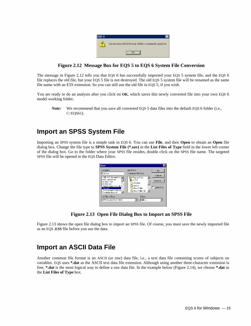
EQS 6 for Windows — 15
Figure 2.12 Message Box for EQS 5 to EQS 6 System File Conversion The message in Figure 2.12 tells you that EQS 6 has successfully imported your EQS 5 system file, and the EQS 6 file replaces the old file, but your EQS 5 file is not destroyed. The old EQS 5 system file will be renamed as the same file name with an E5S extension. So you can still use the old file in EQS 5, if you wish. You are ready to do an analysis after you click on OK, which saves this newly converted file into your own EQS 6 model working folder.
Note: We recommend that you save all converted EQS 5 data files into the default EQS 6 folder (i.e., C:\EQS61).
Import an SPSS System File Importing an SPSS system file is a simple task in EQS 6. You can use File, and then Open to obtain an Open file dialog box. Change the file type to SPSS System File (*.sav) in the List Files of Type field in the lower left corner of the dialog box. Go to the folder where your SPSS file resides, double click on the SPSS file name. The targeted SPSS file will be opened in the EQS Data Editor.
Figure 2.13 Open File Dialog Box to Import an SPSS File Figure 2.13 shows the open file dialog box to import an SPSS file. Of course, you must save the newly imported file as an EQS .ESS file before you use the data.
Import an ASCII Data File Another common file format is an ASCII (or raw) data file, i.e., a text data file containing scores of subjects on variables. EQS uses *.dat as the ASCII text data file extension. Although using another three-character extension is fine, *.dat is the most logical way to define a raw data file. In the example below (Figure 2.14), we choose *.dat in the List Files of Type box.

16 — EQS 6 for Windows
Figure 2.14 Open File Dialog Box for ASCII Data Files Double click on the file name chatter.dat in this dialog box. Alternatively, you can click the file name and then click the OK button to open this raw data file. After double-clicking on the name of the file, or clicking the OK button, you will see the Raw Data File Information dialog box in Figure 2.15.
Figure 2.15 Raw Data File Information Dialog Box
Format The Raw Data File Information dialog box in Figure 2.15 requires information on the format of your data file. It is assumed that the data are organized in such a way that one or more rows or records of the file describe case number 1, across all variables. Following case number 1 is case number 2, and so on. You can also specify a format to read the data in the file. There are two possible types of format:
• Free format • Fixed format
Free Format
A data file in free format has at least one delimiter between the numerical values of adjacent variables. The delimiter can be a space, a tab, a comma and a space, or any character that you specify. If your data file is in free format, chose the radio button that matches the way your file was written. You have no need for Format Builder. When you need detailed information on the fixed format option using Fixed format, read Data Import and Export, Chapter 4. If your data file contains only variable data separated by a space, you can simply accept the default, Space. The number of lines per case is vital to EQS in analyzing the data. In addition to the number of lines per case, you can specify the character that designates missing values.

EQS 6 for Windows — 17
Free Format Example For chatter.dat, accept the defaults of Space and Lines per Case =1. Click OK. The String prompt box in Figure 2.16 appears.
Figure 2.16 String Prompt Box
EQS 6 for Windows found a string in the first case of the chatter.dat data file, so you see the String Prompt box. You get this box because EQS can read complex ASCII files in which the first case actually contains the variable names. If you did not want EQS to treat the string as variable labels, you would click No. However, since the first case contains the names of the variables in chatter.dat, click Yes, and the data file appears.
Data File in Data Editor
Actually, the file that you see in the Data Editor is a copy of the raw data file, so that your original file remains intact. This file is named chatter.ess, since it is now treated as a system file. The file appears on your screen with default variable names: VAR1, VAR2, VAR3, etc. Typically, you would now go to the Data menu and pull down the Information dialog box so that you could assign some identifying labels to the variables. But we shall save that step for later. (You can, of course, explore it now by yourself.) Figure 2.17 shows the file brought up in the EQS Data Editor.
Figure 2.17 Chatter.ess in EQS 6 for Windows Data Editor The rows along the left give the subject, or case, numbers. The columns give the default variable names, VAR1, VAR2, and so on. Each entry, of course, gives the raw data score of a case on a variable.
Note: A data file must be visible and active before you can perform any meaningful function.

18 — EQS 6 for Windows
We have purposely created the EQS 6 for Windows program to be data-oriented. All procedures available in EQS 6 for Windows are based on a dataset being available in the Data Editor. Thus, you must have an open dataset in the Data Editor in order to continue processing. If you have no data in an existing file, you must create a new data file by clicking the File menu, selecting New, and typing in the numbers yourself. These numbers are entered cell by cell into the spreadsheet Data Editor so that the data file resembles Figure 2.17. After you import the ASCII data file in the EQS Data Editor, you should save the data before you perform any analysis.
Step 3: Activate a Program Function To activate a program function, we first open a data file. Retrieve the fisher.ess file by going to the File menu, selecting Open, and clicking on fisher.ess. This file contains 150 rows of numbers, along with a label for each of the variables. Previously, someone entered these labels via the Data menu, using the Information selection. The EQS program permits a variety of data-analytic procedures and manipulations, but here we will start with an example based on a histogram. Later we will turn to a regression analysis and build an EQS model.
Plotting a Histogram After you have opened a data file, you can access many data manipulation procedures easily. Please note that there are 21 icons in the EQS 6 for Windows toolbar. These icons are displayed in Figure 2.18:
Figure 2.18 EQS 6 for Windows Plot Function Icons
The first 7 icons are the most frequently used Windows functions. Next are Diagrammer and the missing data plot icon. The remaining 12 icons are various plot tools. Each icon in the tool bar has a tool tip associated with it. When you position your mouse cursor on the tool icon for a few seconds, the tool tip will pop up telling you the icon’s function. Let’s choose the third plot option, the histogram, from the group of plot tools. A histogram provides a nice graphical way of showing the distribution of scores on a variable. A histogram also provides visual information that is relevant to evaluating model assumptions such as normality.
Use your mouse to move the selector arrow to the histogram icon tool and click on it. The dialog box that serves the histogram option will open, as shown in Figure 2.19 below. You will see some options that we need not use here.
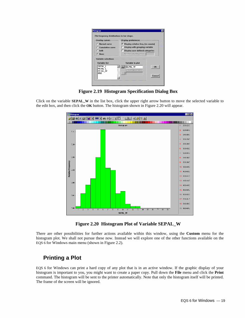
EQS 6 for Windows — 19
Figure 2.19 Histogram Specification Dialog Box Click on the variable SEPAL_W in the list box, click the upper right arrow button to move the selected variable to the edit box, and then click the OK button. The histogram shown in Figure 2.20 will appear.
Figure 2.20 Histogram Plot of Variable SEPAL_W
There are other possibilities for further actions available within this window, using the Custom menu for the histogram plot. We shall not pursue these now. Instead we will explore one of the other functions available on the EQS 6 for Windows main menu (shown in Figure 2.2).
Printing a Plot EQS 6 for Windows can print a hard copy of any plot that is in an active window. If the graphic display of your histogram is important to you, you might want to create a paper copy. Pull down the File menu and click the Print command. The histogram will be sent to the printer automatically. Note that only the histogram itself will be printed. The frame of the screen will be ignored.

20 — EQS 6 for Windows
You might want to use a plot in a different program, such as a word processor. There are two methods that you could use to bring a plot from EQS to another program.
1. You can use the Copy option in the plot window (i.e., the icon with the camera shape) to copy the plot to the clipboard. You can then Paste the plot into the new document.
2. You can use the File menu Save option to create a graphics file for import into other programs. EQS can export plot windows in two formats. They are BMP (a standard bitmap) and WMF (Windows Metafile Format).
Summary The above steps of reading a dataset, saving the raw data in an EQS system file, generating the histogram, and getting a hard copy of the plot have taken a few pages to describe. However, the entire process takes only a few clicks or double clicks of the mouse, and very few keyboard actions. You will find, in general, that the choices EQS gives you are clear to you at all times. While you should know what you are attempting to do with your data, you need to remember very little about the program itself. EQS 6 for Windows aims to be easy and intuitive no matter what you want to accomplish. Doing statistics, you will see, can be fun!
Discarding Windows and Files If you have been following this tutorial carefully, you will now have three screens available for study and analysis. The number and their content are shown in the Window menu. However, this is a good place to point out that you can have a maximum of 12 windows active at once. It is usually worthwhile to close or discard datasets and windows you no longer need.
You can save and close most datasets. After you save a dataset as a file, click on the EQS icon in the upper left corner of the dataset window, and then click on Close to close the window. That dataset is removed from active memory and removed from the list in Window.
You can save plots by using the File menu Save option. You can also print or discard plots. To discard a plot, close its screen. When you close the plot screen, that screen disappears from active memory and from the Window menu.
A Multiple Regression Analysis Now we can turn to one of the most widely used methods for data analysis, linear regression. A standard problem in data analysis is predicting the scores on one variable from the scores on other variables. This is a problem in multiple regression. To illustrate the method, we will use an EQS system file called airpoll.ess. As usual, you must open the data file.
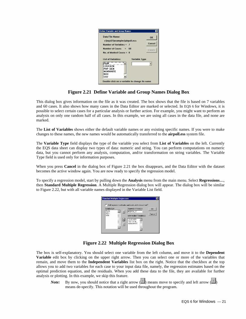
At this point, the data file is placed into the active window, and you can proceed to the analysis. So far we have not told you what information the airpoll.ess dataset actually contains. In order to find out, you should open the data information dialog box. To get it, you pull down the Data menu and select Information. The dialog box in Figure 2.21 will appear.
EQS 6 for Windows — 21
Figure 2.21 Define Variable and Group Names Dialog Box
This dialog box gives information on the file as it was created. The box shows that the file is based on 7 variables and 60 cases. It also shows how many cases in the Data Editor are marked or selected. In EQS 6 for Windows, it is possible to select certain cases for a particular analysis or further action. For example, you might want to perform an analysis on only one random half of all cases. In this example, we are using all cases in the data file, and none are marked.
The List of Variables shows either the default variable names or any existing specific names. If you were to make changes to these names, the new names would be automatically transferred to the airpoll.ess system file. The Variable Type field displays the type of the variable you select from List of Variables on the left. Currently the EQS data sheet can display two types of data: numeric and string. You can perform computations on numeric data, but you cannot perform any analysis, computation, and/or transformation on string variables. The Variable Type field is used only for information purposes. When you press Cancel in the dialog box of Figure 2.21 the box disappears, and the Data Editor with the dataset becomes the active window again. You are now ready to specify the regression model.
To specify a regression model, start by pulling down the Analysis menu from the main menu. Select Regressions…, then Standard Multiple Regression. A Multiple Regression dialog box will appear. The dialog box will be similar to Figure 2.22, but with all variable names displayed in the Variable List field.
Figure 2.22 Multiple Regression Dialog Box The box is self-explanatory. You should select one variable from the left column, and move it to the Dependent Variable edit box by clicking on the upper right arrow. Then you can select one or more of the variables that remain, and move them to the Independent Variables list box on the right. Notice that the checkbox at the top allows you to add two variables for each case to your input data file, namely, the regression estimates based on the optimal prediction equation, and the residuals. When you add these data to the file, they are available for further analysis or plotting. In this example, we skip this feature.
Note: By now, you should notice that a right arrow ( ) means move to specify and left arrow ( ) means de-specify. This notation will be used throughout the program.

22 — EQS 6 for Windows
We will do a simple regression using MORTALIT as the dependent variable to be predicted. Search the Variable List until you find it, then click on the upper right arrow ( ) button. Then select EDUCATN, POP_DEN, and NONWHITE as the independent, or predictor, variables, and click on the lower right arrow button.
Note: To select multiple noncontiguous variables from the list, hold down the <Ctrl> key while clicking on each variable. To select multiple contiguous variables from the list, drag the cursor over each variable, or hold down the <Shift> key while clicking on each variable.
After you specify these variables with mouse clicks, click the OK button to run the regression analysis program. After you press OK, wait a few moments. A message box will pop up to inform you that the analysis is done. Click OK, and you can review the regression analysis output. As stated above, the output of all statistical computations in EQS 6 for Windows is stored in an output file. The name of this output file bears the format of “data file name”+”date and time of the day”. Thus, each of this output file is unique. This file opens automatically when the EQS program starts, though it is empty until you do an analysis. However, at the end of a computation, this output file will automatically become the active window. You can scroll through the output to examine the results of your analysis.
These output files are all stored in C:\EQS61\OUTPUT\ folder. You can access them using a text editor like EQS 6.1’s text editor or Windows Notepad, The output file has three parts, consisting of:
1. Summary of variables and cases used 2. Analysis of variance of the regression 3. Statistics for the regression
Figure 2.23 shows the output .log displaying test statistics for each independent variable, including unstandardized regression coefficient, ordinary standard errors, heteroscedastic standard errors, standardized coefficient, t-value, and p-value.
STANDARD MULTIPLE REGRESSIONS 4 Variables are selected from file c:\eqs61\examples\airpoll.ess Number of cases in data file are ........... 60 Number of cases used in this analysis are .. 60 ANALYSIS OF VARIANCE ==================== Source SUM OF SQUARES DF MEAN SQUARES F p ___________________________________________________________________ REGRESSION 135854.579 3 45284.860 27.416 0.000 RESIDUAL 92498.190 56 1651.753 TOTAL 228352.770 59 ___________________________________________________________________ Dependent Variable = MORTALIT Number of obs. = 60 Multiple R = 0.7713 R-square = 0.5949 Adjusted R-square = 0.5732 F( 3, 56) = 27.4162 Prob > F = 0.0000 Std. Error of Est. = 40.6418 Durbin-Watson Stat.= 1.7809 =======REGRESSION COEFFICIENTS======= HETERO- ORDINARY SCEDASTIC VARIABLE B STD. ERROR STD. ERROR BETA t p ____________________________________________________________________________ Intercept 1142.047 79.230 94.778 12.050 0.000 EDUCATN -25.507 6.598 8.801 -0.347 -2.898 0.005 POP_DEN 0.008 0.004 0.007 0.187 1.179 0.243 NONWHITE 4.000 0.608 0.710 0.574 5.637 0.000 ____________________________________________________________________________
Figure 2.23 An Example of Regression output

EQS 6 for Windows — 23
For the sake of brevity, this concludes the regression example. Let us now turn to a structural equation model.
Step 4: Create and Run an EQS Model EQS 6 has an advanced model-building facility to help you build some standard models. You only need to specify the relationship between variables in the form of dependent-independent variables and/or correlations. Based on the type of model you want to create, EQS will build the diagram for you. Let’s try some of these exciting features:
A Path Analysis Model
The path model is a commonly used model that can be built easily. The model is actually a simultaneous equations model with some correlation among independent variables. Let’s use the dataset manul4.ess. The dataset contains 6 variables and 932 observations (see Figure 2.24). We have edited the variable names in the dataset so that they are meaningful. You can click on Data and then Information to customize variable names. Detailed information on customizing variable names will be discussed elsewhere in this manual.
Figure 2.24 Test Dataset to Create a Path Model Let’s start building the path model, which is the model described in EQS 6 Structural Equations Program Manual. In the data window, you must click File, and then New and change the file type to Diagram File (*.EDS) which will open a blank diagram window, or else click on the Diagrammer icon on the toolbar as shown in Figure 2.25 to activate New Model Helper. The latter is simpler, so we click on it now.
or
Figure 2.25 New Diagram Window or Diagrammer to Activate New Model Helper
Build a Path Model As you can see in Figure 2.26, the New Model Helper contains four picture buttons and a Cancel button. Each of the first three picture buttons contains a series of procedures to help you create an EQS model. The fourth one, “Diagram Window”, opens a blank diagram window for you to draw a new diagram. Since we want to create a path model

24 — EQS 6 for Windows
now, let’s click on the top picture icon. A note on the dialog box tells you that it is a one-step process to build a path model.
Figure 2.26 New Diagram Window Options You will be shown a Path Model Builder dialog box as shown in Figure 2.27. This dialog box contains three parts. The far left section is the list of all variables in the data file. The middle section is a regression specifier. The far right section is the path model. The unique feature of a path model is that all the variables used in the model are measured variables. There are three steps in this dialog box. Step 1: You must specify a dependent variable from the variable list on the left side of the dialog box, and click
on the top right arrow ( ) button to move the variable to the Dependent Variable edit box. Step 2: After the dependent variable is specified, you must select the independent variables from the variable
list box and move them to the Its Predictors list box (press the <Ctrl> key and click on the variables in the variable list box if you want to select a number of non-contiguous variables), by using the lower right arrow button.
Step 3: After moving all of the predictors of this dependent variable, use the Add button to move the regression
equation to the Path Model section on the right hand side. Repeat steps 1 - 3 until all regression equations are moved to the Path Model section. You have completed the process of building a path model. These equations are your path model. Click on the OK button, and you will see that EQS opens a diagram window and puts the path model you have specified in the window (see Figure 2.28). Our path model has two equations: ANOMIE71 = *ANOMIE67 + *POWRLS67 + error; POWRLS71 = *ANOMIE67 + *POWRLS67 + error; To build such a model, we first click on ANOMIE71 and move it to the Dependent Variable box. Then we select ANOMIE67 and POWRLS67 and move them to the Its Predictors list. The first equation is complete, so we click on the Add button, and the first equation is moved to the Path Model section. For the second equation, we click on POWRLS71 and move it to the Dependent Variable box. For independent variables, we select both ANOMIE67 and POWRLS67 and move them to the Its Predictors list box. Click on the Add button to add the second equation to the Path Model section.

EQS 6 for Windows — 25
The path model building process is complete and we should click on the OK button. The model is created as shown in Figure 2.28. (Note that this model was prepared for this manual. Your screen version will have shading.)
Figure 2.27 Path Model Builder Dialog Box
POWRLS67
ANOMIE71ANOMIE67
POWRLS71 E4
E3
Figure 2.28 Path Model Created by New Model Helper
The path model you are specifying has been built on the Diagrammer with very little effort. You are ready to run EQS based on the model you just built.
Run the Path Model You finish building the EQS model from the diagram shown in Figure 2.28 by using a few more clicks. While on the diagram window (please note that both your data and diagram are active at this point), pull down the Build_EQS menu and select Title/Specifications. Before EQS runs the model, you will be asked to save the model file in a dialog box shown as Figure 2.29. You have to save the model file for EQS to continue.
Figure 2.29 Save As Dialog Box to Save the Diagram File After you save the diagram file, an EQS model file window will open with an EQS model listed on the window then EQS Model Specifications dialog box (Figure 2.30) appears.

26 — EQS 6 for Windows
Figure 2.30 EQS Specification Dialog Box In this EQS Specification Dialog Box, the data file name has been set and the estimation method is given. Most of the model’s input information has been provided. You are ready for the next step, so click on the OK button in the EQS Model Specifications dialog box. You will now be on the EQS Model file window where there are EQS commands on the screen associate with the path diagram you just created in Diagrammer as shown in Figure 2.31. Please note that this EQS Model file appears to be a text file but it is not. You could modify the contents of the model only through the sub-menus in Build_EQS menu. The model in this point is ready to run.
/TITLE EQS model created by EQS 6 for Windows -- c:\eqs6\examples\manul4.eds /SPECIFICATIONS DATA='c:\eqs61\examples\manul4.ess'; VARIABLES=6; CASES=932; GROUPS=1; METHODS=ML; MATRIX=CORRELATION; ANALYSIS=COVARIANCE; /LABELS V1=ANOMIE67; V2=POWRLS67; V3=ANOMIE71; V4=POWRLS71; V5=V5; V6=V6; /EQUATIONS V3 = + *V1 + *V2 + 1E3; V4 = + *V1 + *V2 + 1E4; /VARIANCES V1 = *; V2 = *; E3 = *; E4 = *; /COVARIANCES V2 , V1 = *; /PRINT EIS; FIT=ALL; TABLE=EQUATION; /STANDARD DEVIATION /MEANS /END
Figure 2.31 A Path Model Command File Built by the Build_EQS Process
Go back to the Build_EQS menu, pull it down and select the Run EQS option to run it. You will be asked again to save the EQS model file as the dialog box looks like Figure 2.29 with EQS Model File (*.EQX) as the file extension. After you click on the Save button, EQS will start to run. Depending on the speed of your computer, the EQS running status will be displayed briefly until it is done. The output of EQS will be automatically fetched to the front window for you to examine. We will not show the EQS output here. Detailed information on EQS output will be provided and illustrated in EQS 6 Structural Equations Program Manual.

EQS 6 for Windows — 27
A Confirmatory Factor Analytic Model Let’s build a confirmatory factor analysis model, using an example from the EQS 6 Structural Equations Program Manual. It uses a raw score dataset called manul7a.ess, which is stored as an EQS system file. This data file has six variables. We want to show you how to build a six-variable, two-factor confirmatory factor model. We will develop the model based on the raw data. If the file contained the covariance or correlation matrix for these data, we would use a virtually identical procedure. First, of course, you have to activate the EQS 6 for Windows program if it is not already active, and open the appropriate data file. Pull down the File menu from the main menu and select the Open option to get an open file dialog box. The dialog box shows the list of files. Select manul7a.ess, then click OK or press the <Enter> key, or double-click manul7a.ess to bring the file to the Data Editor. After deciding on the dataset, we can start building the EQS model. To build an EQS model in the conventional way, you type in the equations, variances, and covariances, character by character using a text editor. EQS 6 for Windows provides two more advanced ways to build the equations.
1. The Building an EQS Model Using the Diagrammer section of this chapter
illustrates how you can build a model by simply drawing a diagram on the screen and letting the program generate the model for you.
2. The Building an EQS Model by Using Equation Table section of this chapter shows that you can create a table consisting of the components of the equations. Then fill in the free parameters by clicking on cells with your mouse.
Either method will substantially reduce the time required to build a model, compared to other methods.
1. Building an EQS Model Using the Diagrammer You must open the New Model Helper to build the new model. To do this, click the Diagrammer icon (shown on the right side of Figure 2.25) from the tool bar. You will see New Model Helper (shown in Figure 2.26). Click on the second picture button that shows Factor Model. You will see a series of dialog boxes, which will help you create the factor model. These dialog boxes are
1. Dialog box to specify all factor structures 2. Dialog box to specify all structural equations 3. Dialog box to specify all factor correlations
The first dialog box accepts factor loading specifications. It allows you to obtain all factor structures by providing their indicators. The dialog consists of three main parts. The left hand side is a Variable List box. The middle section is a Factor Structure box, and the right hand side is a Model Components group box. You create a factor structure by moving a factor’s indicators from the Variable List to the middle Indicators box. When one factor is done, you add it the Model Components section on the right hand side of the dialog box. Repeat this process until all factor structures are created. In this example, you will select V1, V2, and V3 and click on the right arrow button to move them to the Indicators box. Click on the Add button to create the first factor structure. Next, select V4, V5, and V6, click on the right arrow button to move them into the indicator list and click on the Add button to create the second factor structure. Click on Next, which brings up Step 2.
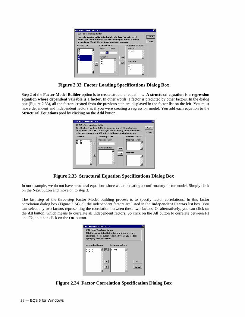
28 — EQS 6 for Windows
Figure 2.32 Factor Loading Specifications Dialog Box Step 2 of the Factor Model Builder option is to create structural equations. A structural equation is a regression equation whose dependent variable is a factor. In other words, a factor is predicted by other factors. In the dialog box (Figure 2.33), all the factors created from the previous step are displayed in the factor list on the left. You must move dependent and independent factors as if you were creating a regression model. You add each equation to the Structural Equations pool by clicking on the Add button.
Figure 2.33 Structural Equation Specifications Dialog Box
In our example, we do not have structural equations since we are creating a confirmatory factor model. Simply click on the Next button and move on to step 3.
The last step of the three-step Factor Model building process is to specify factor correlations. In this factor correlation dialog box (Figure 2.34), all the independent factors are listed in the Independent Factors list box. You can select any two factors representing the correlation between these two factors. Or alternatively, you can click on the All button, which means to correlate all independent factors. So click on the All button to correlate between F1 and F2, and then click on the OK button.
Figure 2.34 Factor Correlation Specification Dialog Box

EQS 6 for Windows — 29
You will see a diagram window with a two-factor CFA model (Figure 2.35). You are nearly ready to run this model.
E6
V1
V2
V3
F1
E1
E2
E3
V4
V5
V6
F2
E4
E5
Figure 2.35 Two-Factor CFA Model
Build EQS Model
Now that you have opened the data file and drawn the diagram, you are ready to finish building the EQS model. Click the Build_EQS selection from the main menu. You can see from the drop-down menu that there are many items in this menu, but only two items are black and active. (The remaining options are grayed out and inactive.) This choice of only two options indicates that you should start with the item on top of the menu, Title/Specifications, to build an EQS model. By selecting this option, you can see a new dialog box:
Note: You will be asked to save the diagram before the EQS Model Specifications dialog box
appears. EQS 6 uses data file name plus .eds as the extension as the default diagram file name. We recommend you use the default name since this name coincides with your data file name (except for the extension .eds).
Figure 2.36 EQS Model Specifications
Figure 2.37 Additional Options The new dialog box called EQS Model Specifications will appear as shown in Figure 2.36. This box has the information required in the /SPECIFICATIONS paragraph of the EQS program. By default, the EQS Model Specifications box automatically has most of the information you need to specify a model. Some of the default information is from the *.ess file (here, manul7a.ess), and some reflects choices typically made in structural
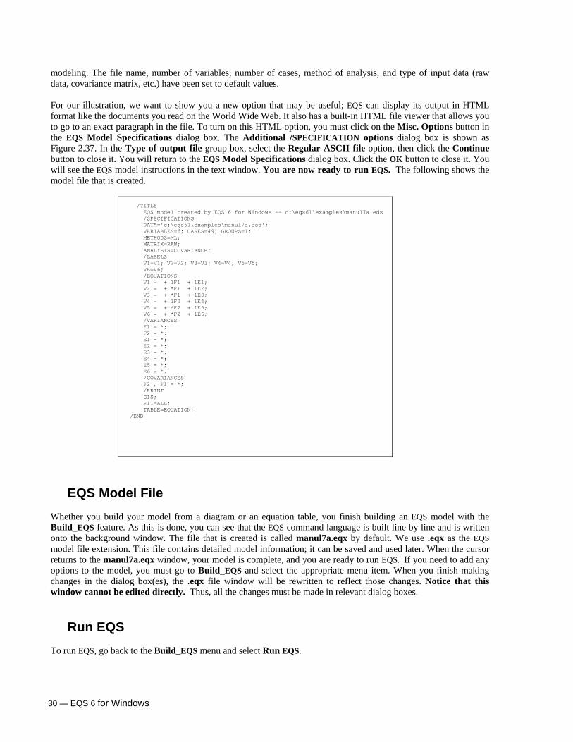
30 — EQS 6 for Windows
modeling. The file name, number of variables, number of cases, method of analysis, and type of input data (raw data, covariance matrix, etc.) have been set to default values.
For our illustration, we want to show you a new option that may be useful; EQS can display its output in HTML format like the documents you read on the World Wide Web. It also has a built-in HTML file viewer that allows you to go to an exact paragraph in the file. To turn on this HTML option, you must click on the Misc. Options button in the EQS Model Specifications dialog box. The Additional /SPECIFICATION options dialog box is shown as Figure 2.37. In the Type of output file group box, select the Regular ASCII file option, then click the Continue button to close it. You will return to the EQS Model Specifications dialog box. Click the OK button to close it. You will see the EQS model instructions in the text window. You are now ready to run EQS. The following shows the model file that is created.
/TITLE EQS model created by EQS 6 for Windows -- c:\eqs61\examples\manul7a.eds /SPECIFICATIONS DATA='c:\eqs61\examples\manul7a.ess'; VARIABLES=6; CASES=49; GROUPS=1; METHODS=ML; MATRIX=RAW; ANALYSIS=COVARIANCE; /LABELS V1=V1; V2=V2; V3=V3; V4=V4; V5=V5; V6=V6; /EQUATIONS V1 = + 1F1 + 1E1; V2 = + *F1 + 1E2; V3 = + *F1 + 1E3; V4 = + 1F2 + 1E4; V5 = + *F2 + 1E5; V6 = + *F2 + 1E6; /VARIANCES F1 = *; F2 = *; E1 = *; E2 = *; E3 = *; E4 = *; E5 = *; E6 = *; /COVARIANCES F2 , F1 = *; /PRINT EIS; FIT=ALL; TABLE=EQUATION;
/END
EQS Model File Whether you build your model from a diagram or an equation table, you finish building an EQS model with the Build_EQS feature. As this is done, you can see that the EQS command language is built line by line and is written onto the background window. The file that is created is called manul7a.eqx by default. We use .eqx as the EQS model file extension. This file contains detailed model information; it can be saved and used later. When the cursor returns to the manul7a.eqx window, your model is complete, and you are ready to run EQS. If you need to add any options to the model, you must go to Build_EQS and select the appropriate menu item. When you finish making changes in the dialog box(es), the .eqx file window will be rewritten to reflect those changes. Notice that this window cannot be edited directly. Thus, all the changes must be made in relevant dialog boxes.
Run EQS To run EQS, go back to the Build_EQS menu and select Run EQS.

EQS 6 for Windows — 31
Before the program actually runs the EQS job, it displays a Save As dialog box as in Figure 2.30. For safety’s sake, you should save your EQS model file before running it. We have been working on the manul7a.ess data, you have saved the diagram file as manul7a.eds, and thus the default file name for the EQS model is manul7a.eqx. In naming your diagram file, be sure to select a file name that will remind you of your data file name.
The output from the run will be named manul7a.htm. If you had not chosen HTML output, you would have your specified file name, with the *.out extension. So, work.eqx will yield work.out as the output file, and manul7a.eqx will yield manul7a.out.
Examine the EQS Output File
When the EQS model run is complete, the output is automatically sent to the front window. If you chose to display a regular ASCII output, the output file will be displayed in a text editor. You can scroll up and down. You can even use the Find/Replace function to locate specific information. If, however, you requested an output file in HTML format (as in this example), the output file will be placed in the HTML file viewer. You can click on the pre-defined topics to position the output to the exact paragraph you want to read. The first part of the output will echo your input file, so that you can verify what job was actually run. Beyond that, the output file includes all the standard results from a structural modeling run. We do not describe this output any further, because it is fully documented in the EQS 6 Structural Equations Program Manual.
Examine EQS Output on the Diagram If you have created the EQS model using the diagram method, the parameter estimates will be brought to the diagram when the job is done. When building an EQS model file using a diagram, the program will insert an EIS command into the /PRINT section automatically. The EIS command will write all estimates to an external file called input_file_name.eis. The Diagrammer can read those estimates later, after the EQS job is done. To review the parameter estimates from the diagram, choose the Window menu and select the diagram file name (i.e., manul7a.eds). The diagram window will appear with some basic statistics displayed at the bottom of the diagram window. If you want to see the estimates of each parameter, click the View menu and select Estimates and Parameter estimates. The diagram window will be redrawn with parameter estimates embedded in the paths (Figure 2.38).
Figure 2.38 Path Diagram with Embedded Parameter Estimates Now close the diagram window, and let’s try doing the same thing a different way.
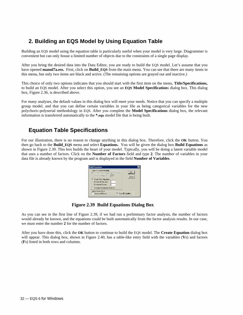
32 — EQS 6 for Windows
2. Building an EQS Model by Using Equation Table Building an EQS model using the equation table is particularly useful when your model is very large. Diagrammer is convenient but can only house a limited number of objects due to the constraints of a single page display. After you bring the desired data into the Data Editor, you are ready to build the EQS model. Let’s assume that you have opened manul7a.ess. First, click on Build_EQS from the main menu. You can see that there are many items in this menu, but only two items are black and active. (The remaining options are grayed out and inactive.) This choice of only two options indicates that you should start with the first item on the menu, Title/Specifications, to build an EQS model. After you select this option, you see an EQS Model Specifications dialog box. This dialog box, Figure 2.36, is described above. For many analyses, the default values in this dialog box will meet your needs. Notice that you can specify a multiple group model, and that you can define certain variables in your file as being categorical variables for the new polychoric-polyserial methodology in EQS. After you complete the Model Specifications dialog box, the relevant information is transferred automatically to the *.eqx model file that is being built.
Equation Table Specifications For our illustration, there is no reason to change anything in this dialog box. Therefore, click the OK button. You then go back to the Build_EQS menu and select Equations. You will be given the dialog box Build Equations as shown in Figure 2.39. This box builds the heart of your model. Typically, you will be doing a latent variable model that uses a number of factors. Click on the Number of Factors field and type 2. The number of variables in your data file is already known by the program and is displayed in the field Number of Variables.
Figure 2.39 Build Equations Dialog Box As you can see in the first line of Figure 2.39, if we had run a preliminary factor analysis, the number of factors would already be known, and the equations could be built automatically from the factor analysis results. In our case, we must enter the number 2 for the number of factors. After you have done this, click the OK button to continue to build the EQS model. The Create Equation dialog box will appear. This dialog box, shown in Figure 2.40, has a table-like entry field with the variables (Vs) and factors (Fs) listed in both rows and columns.

EQS 6 for Windows — 33
Figure 2.40 Create Equation Dialog Box
Each row corresponds to a dependent variable in your path diagram, i.e., a variable with one or more one-way arrows aimed at it. Thus, each row corresponds to a possible equation that you might build. Each column gives one of the possible predictors of that variable. There are three simple ways to specify your equations.
1. Use your mouse to click on each aqua-colored cell that should be a free parameter in the model.
As you click on a cell, an asterisk will appear. 2. As an alternative, you can use click and drag. Position your mouse pointer in the upper left cell,
inside the cell defined by V1 and F1. Click your mouse button, and hold down the button and drag the pointer so that it terminates in the V3,F1 cell. The idea is to cover the top three cells under F1 by an active rectangle. Now, release your mouse button. You will see a dialog box Start Value Specifications (Figure 2.41). The default radio button is set to Fix one and free others. This option allows you to fix the first factor loading at one and free the other loadings if you have covered more than one factor loading. This dialog box also allows you to specify other types of models (e.g. latent growth curve model) with ease. Click OK to continue, then select with your mouse an active rectangle covering the V4, V5, V6 cells under F2. Click OK in the Start Value Specifications box, and your table will look exactly like Figure 2.40.
Figure 2.41 Start Value Specifications Dialog Box
3. You can double-click on any cell. The cell will change color to yellow and the cursor will appear in the cell. You can add and/or change the start value in the cell and end the start value with an asterisk (*) if it is a free parameter. To enter your changes, you must type a tab, an Enter key, or double click on another cell.
In this example, we use the default start value option. Variables V1-V3 are indicators of Factor 1, and V4-V6 are indicators of Factor 2. Make the relevant selections now. If you make a mistake, you can click again on a cell to unselect a previously-selected parameter. You should get a result that looks like Figure 2.40.

34 — EQS 6 for Windows
Each asterisk in a cell represents a free parameter in your model. The unmarked factor loadings are automatically fixed at zero by the program. This completes the setup of equations. When the dialog box looks like Figure 2.40, Press OK.
Variance/Covariance Table Specifications Of course, a model must include variances and covariances of independent variables as well as equations. Next we specify these parameters. The Create Variance/Covariance dialog box appears automatically, as shown in Figure 2.42.
Figure 2.42 Create Variances/Covariances Dialog Box In this box, blank entries are parameters fixed at zero, while entries that will become free parameters must be specified with an asterisk. The diagonals of this matrix represent the variances of the variables, while the off-diagonals deal with the covariances or correlations between pairs of variables. When the dialog box appears on the screen, the independent variables from the equations box, plus the implied residual variables, are shown as the independent variables in the model. Each diagonal cell contains an asterisk, indicating that the variances of F1, F2, E1, ..., E6 are taken to be free parameters. This may or may not be the correct specification that you have in mind, so you should adjust the box to meet your specific model needs. Since we have fixed one of the factor loadings for each factor, we need not do anything to the variances. We want to let the two factors correlate, so we place an asterisk in the F2,F1 cell. The result will look like Figure 2.42. (We could also have made these three changes at once by moving the pointer above and left of the F1,F1 position, clicking, dragging into the E1,E1 position, and then releasing.) Now that we are finished making the variance and covariance specifications, press the OK button.
EQS Model File Whether or not you build your model from a diagram or an equation table, you finish building an EQS model with the Build_EQS feature. As this is done, you can see that the EQS command language is built line by line and is written onto the background window. The file that is created is called manul7a.eqx by default. The following shows the model file that is created.

EQS 6 for Windows — 35
/TITLE EQS model created by EQS 6 for Windows -- manul7a.ESS /SPECIFICATIONS DATA='c:\eqs61\examples\Manul7a.ess'; VARIABLES=6; CASES=49; GROUPS=1; METHODS=ML; MATRIX=RAW; ANALYSIS=COVARIANCE; /LABELS V1=V1; V2=V2; V3=V3; V4=V4; V5=V5; V6=V6; /EQUATIONS V1 = + 1F1 + 1E1; V2 = + *F1 + 1E2; V3 = + *F1 + 1E3; V4 = + 1F2 + 1E4; V5 = + *F2 + 1E5; V6 = + *F2 + 1E6; /VARIANCES F1 = *; F2 = *; E1 = *; E2 = *; E3 = *; E4 = *; E5 = *; E6 = *; /COVARIANCES F2 , F1 = *; /PRINT FIT=ALL; /END
If you made a mistake in the file, or if you change your mind about any of the specifications, you can move your cursor into the window that contains the manul7a.eqx file. You can modify this file by going back to the Build_EQS menu. Select the menu item for the paragraph you wish to change. You will be given the dialog box associated with the paragraph. Change it, and EQS will update manul7a.eqx automatically.
Run EQS and Examine the EQS Output File
To run EQS, go back to the Build_EQS menu and select Run EQS. Running an EQS model has been discussed previously where we build the model using New Diagram Builder. The EQS output will appear automatically when the job is done. The name of the output file is always the input file name, with .out or .htm replacing .eqx. We do not describe this output any further, because it is fully documented in the EQS 6 Structural Equations Program Manual.
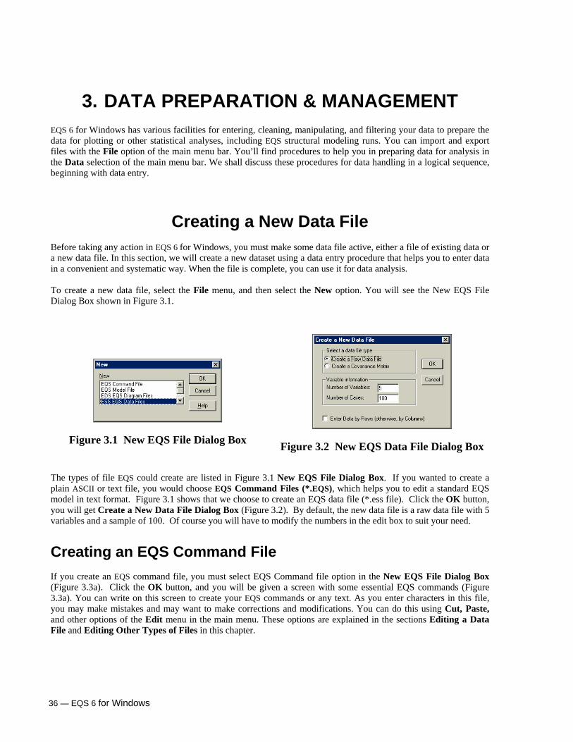
36 — EQS 6 for Windows
3. DATA PREPARATION & MANAGEMENT EQS 6 for Windows has various facilities for entering, cleaning, manipulating, and filtering your data to prepare the data for plotting or other statistical analyses, including EQS structural modeling runs. You can import and export files with the File option of the main menu bar. You’ll find procedures to help you in preparing data for analysis in the Data selection of the main menu bar. We shall discuss these procedures for data handling in a logical sequence, beginning with data entry.
Creating a New Data File Before taking any action in EQS 6 for Windows, you must make some data file active, either a file of existing data or a new data file. In this section, we will create a new dataset using a data entry procedure that helps you to enter data in a convenient and systematic way. When the file is complete, you can use it for data analysis. To create a new data file, select the File menu, and then select the New option. You will see the New EQS File Dialog Box shown in Figure 3.1.
Figure 3.1 New EQS File Dialog Box
Figure 3.2 New EQS Data File Dialog Box
The types of file EQS could create are listed in Figure 3.1 New EQS File Dialog Box. If you wanted to create a plain ASCII or text file, you would choose EQS Command Files (*.EQS), which helps you to edit a standard EQS model in text format. Figure 3.1 shows that we choose to create an EQS data file (*.ess file). Click the OK button, you will get Create a New Data File Dialog Box (Figure 3.2). By default, the new data file is a raw data file with 5 variables and a sample of 100. Of course you will have to modify the numbers in the edit box to suit your need.
Creating an EQS Command File
If you create an EQS command file, you must select EQS Command file option in the New EQS File Dialog Box (Figure 3.3a). Click the OK button, and you will be given a screen with some essential EQS commands (Figure 3.3a). You can write on this screen to create your EQS commands or any text. As you enter characters in this file, you may make mistakes and may want to make corrections and modifications. You can do this using Cut, Paste, and other options of the Edit menu in the main menu. These options are explained in the sections Editing a Data File and Editing Other Types of Files in this chapter.

EQS 6 for Windows — 37
Figure 3.3a New File Dialog Box
Figure 3.3b EQS Command File Template
Creating an EQS System File
To create a raw data file in EQS format, click the File menu and select New. You will be prompted with a New EQS File Dialog Box with the default option set to EQS Command File. You must change to the ESS EQS Data File as shown in Figure 3.4 then click the OK Button.
Figure 3.4 New EQS File Dialog Box to Create ESS File
The Create a New Data File dialog box will appear (Figure 3.5). You may create either a raw data system file or a covariance matrix system file. (For an example of the latter type of file, see the section Create a variance/covariance matrix in Chapter 2.) The default number of variables is 10 and the default number of cases is 100. You must modify these numbers to make them consistent with the number of variables and the number of subjects or cases that you plan to use. In this example, we intend to create a raw data file with 5 variables and 20 cases. So we enter 5 and 20 to the edit boxes labeled Number of Variables and Number of Cases, respectively. You can now select the direction for data entry. The default is Enter Data by Rows, indicated by a check mark in the checkbox labeled Enter Data by Rows (otherwise, by Columns). This option controls the movement of the data entry cursor. If you complete a cell and press the tab key to move forward, the cursor will advance to the cell on the right when this option is checked. Otherwise, the cursor will move to the cell below the current one.
Figure 3.5 Create a New Data File Dialog Box
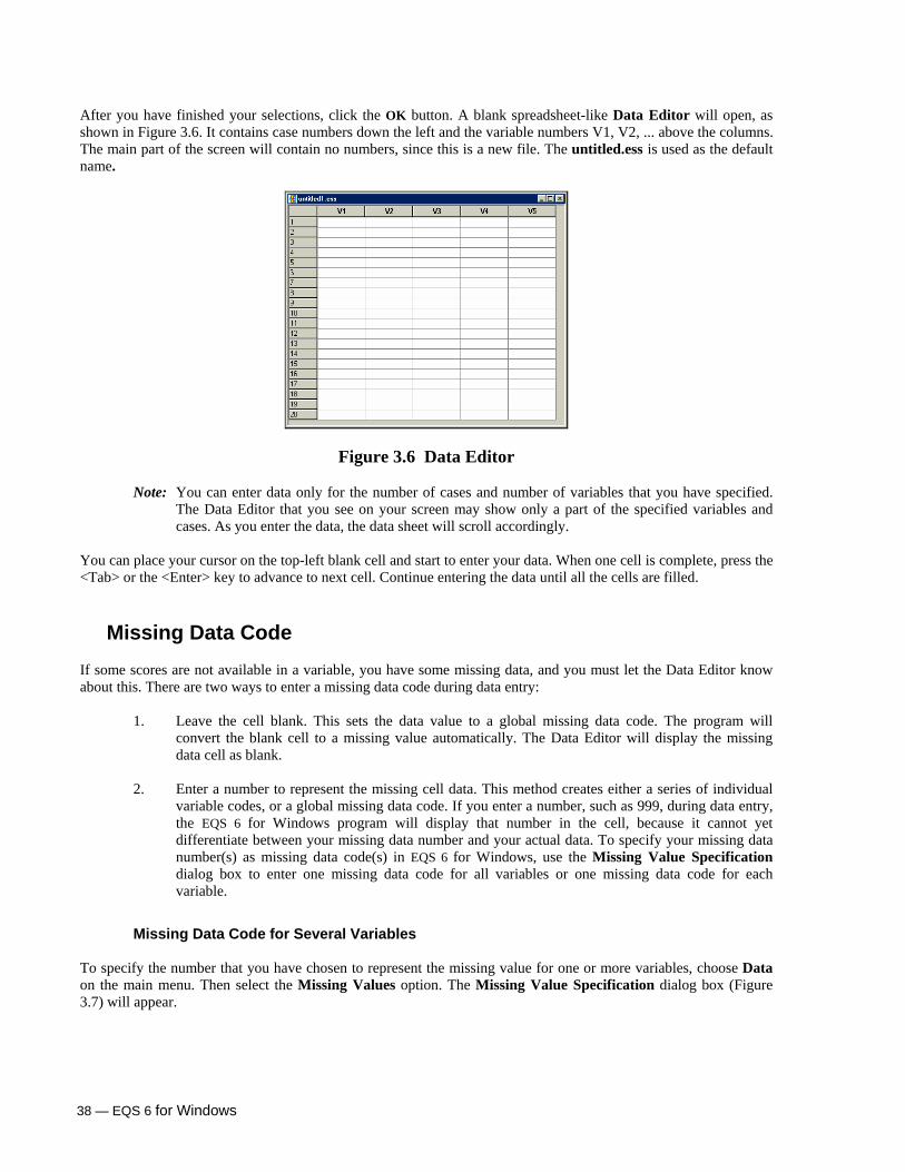
38 — EQS 6 for Windows
After you have finished your selections, click the OK button. A blank spreadsheet-like Data Editor will open, as shown in Figure 3.6. It contains case numbers down the left and the variable numbers V1, V2, ... above the columns. The main part of the screen will contain no numbers, since this is a new file. The untitled.ess is used as the default name.
Figure 3.6 Data Editor
Note: You can enter data only for the number of cases and number of variables that you have specified. The Data Editor that you see on your screen may show only a part of the specified variables and cases. As you enter the data, the data sheet will scroll accordingly.
You can place your cursor on the top-left blank cell and start to enter your data. When one cell is complete, press the <Tab> or the <Enter> key to advance to next cell. Continue entering the data until all the cells are filled.
Missing Data Code If some scores are not available in a variable, you have some missing data, and you must let the Data Editor know about this. There are two ways to enter a missing data code during data entry:
1. Leave the cell blank. This sets the data value to a global missing data code. The program will convert the blank cell to a missing value automatically. The Data Editor will display the missing data cell as blank.
2. Enter a number to represent the missing cell data. This method creates either a series of individual
variable codes, or a global missing data code. If you enter a number, such as 999, during data entry, the EQS 6 for Windows program will display that number in the cell, because it cannot yet differentiate between your missing data number and your actual data. To specify your missing data number(s) as missing data code(s) in EQS 6 for Windows, use the Missing Value Specification dialog box to enter one missing data code for all variables or one missing data code for each variable.
Missing Data Code for Several Variables To specify the number that you have chosen to represent the missing value for one or more variables, choose Data on the main menu. Then select the Missing Values option. The Missing Value Specification dialog box (Figure 3.7) will appear.

EQS 6 for Windows — 39
Figure 3.7 Missing Value Specification Dialog Box In the Select Variable list box, click on a variable to select it. (If all variables have the same missing value, click on the first variable, then hold down the <Shift> key and clicking on the last variable to select all variables.) In the Missing Value Options field, click on the radio button describing your missing value option the best and enter the number representing the missing value for that variable. After you have selected variable(s) and entered the number representing the missing value, click on Apply botton.
Note: When you enter the data, you can see, in any missing data cell on the screen, the number which you have chosen as your missing code. You can still see the missing code after you enter the missing data code for each variable.
Note: Please read the Visualizing and Treating Missing Data section in this chapter for more details on
how EQS 6 for Windows treats missing data.
Editing a Data File After you have created a data file, you may want to edit it. It is always wise to verify that the data were entered correctly, perhaps by comparing a printout of the file as entered with the original source data material. In any case, you may want to change some of the numbers in the file. In this case, go to File, click Open, and select the desired *.ess file from the file list.
When the data matrix window appears, you can refresh your memory concerning file details. Just click on Data in the menu bar, then click on Information. Whether you are creating a new data file, or editing an old data file, EQS 6 for Windows provides some useful file editing options. It allows you to add or delete variables as well as cases. You can search and replace a number within a variable. You can move columns of variables using drag and drop methods. You can undo certain editing functions. To access these edit options, use the File menu Open option to open a data file, and then click on the Edit menu. After making any necessary changes in the file, save it using the File menu Save option.
Undo You can undo most of the edit options. The EQS Undo option allows you to undo up to 12 steps. In other words, the EQS text editor will remember your last 12 steps, and it will undo those steps one by one, beginning with the most recent step.

40 — EQS 6 for Windows
Redo You can redo the steps that were previously undone.
Cut You can cut (erase) a block of highlighted or selected text from the text window. The highlighted text will also be copied to the Windows clipboard, for use in Paste, below. If there is no text highlighted, the Cut function will have no effect. (In fact, the Cut option will be grayed out on the Edit menu.)
Copy You can copy a block of highlighted text into the Windows clipboard, without erasing it from the file. The contents of the clipboard can later be pasted back into the EQS text editor or other programs. Again, if no text is selected in the text editor, the Copy option will be grayed out on the Edit menu.
Paste You can insert the contents of the Windows clipboard into the data file at the position of your cursor. The contents of the clipboard can be created by Cut or Copy, above. When the clipboard is empty, the Paste function is hidden.
Select All This function will select and highlight the entire data sheet.
Fill This function fills a column or a row of cells with a given number.
Clear This function fills the selected cells with blanks.
Insert a Column This function will insert a blank column after the right most columns. You can use this function to add a new variable into your data sheet.
Insert a Row This function will insert a blank row at the end of the data sheet. You can use this function to add a new case to your data.

EQS 6 for Windows — 41
Find The Find function will display a dialog box and ask you to enter a string or a number to be searched (Figure 3.8). You must enter something in the edit box labeled Find what and click on the Find Next button. The Data Editor will locate the particular string or number you are trying to find. The Find function can only be applied to one variable, not the entire contents of the Data Editor.
Figure 3.8 Find Dialog Box
Replace The Replace function will display a dialog box as shown in Figure 3.9. It contains two edit boxes. The first edit box labeled Find what allows you to enter a string or a number to be replaced. The second edit box labeled Replace with will contain the number to replace with. The Replace function can only be applied to one variable, not the entire contents of the Data Editor.
Figure 3.9 Replace Dialog Box
Goto When you click on the Goto option, the Goto Row/Column dialog box (Figure 3.10) will appear. Enter the row and column numbers that you wish to go to, then click on the OK button. The Data Editor will scroll to the row and column number that you are looking for. You will find that both row and column labels will be depressed, and the cell where they intersect is the cell that you specified.
Figure 3.10 Goto/Column Dialog Box
Preference This function allows you to change preferences for EQS model analyses. Please see Chapter 10 for details.

42 — EQS 6 for Windows
Delete Columns and Rows
Although there are no formal commands to allow you to delete columns and rows of data, you could achieve this function by highlighting the rows or columns of the data you want to delete (i.e. click on the header of the rows or columns) then go to Edit->Delete. The highlighted rows or columns will be deleted from the data sheet.
Formatting Your Data You can change the appearance of the EQS Data Editor, e.g. change the size and style of the font. The following section describes these options and how they work. All these formatting options are listed in the View menu of the Data Editor.
Zoom in
Clicking on the Zoom in menu item will increase your font size.
Zoom out
This option will decrease the font size.
100%
This option resets the size of the font in the Data Editor to the default setting. The default font size is 12.
Variable Name
You can toggle the Data Editor back and forth between generic names and symbolic names. Generic names of columns are A, B, C, etc., and cannot be changed. By default, the symbolic names are V1, V2, V3, etc., but you can change the symbolic names of any column(s). See Adding Variable Labels, below.
Formula expression
This option will toggle the Data Editor into a formula sheet. The formula sheet lists all the formulas embedded in each cell if this cell is derived by a formula.
Format Cells
You can modify the appearance of displayed text in the Data Editor. Before formatting a cell, a block of cells, and/or several rows and columns of data, you must select (highlight) them. Then click on the View menu and select Format Cells. You will be provided a dialog box as shown in Figure 3.11.

EQS 6 for Windows — 43
Figure 3.11 Format Cells Dialog Box As you can see from the options in the dialog box, you can change the font, the font size, the outline, the text and background color of a cell, the border, the alignment, and the formats (i.e., decimal places, number sign, dollar sign, integer display, scientific notations, etc).
Format Style
This feature allows you to change the style of the column or row header. When you click on this option, the Styles dialog box will appear (Figure 3.12). You must select one of the three options for further action. Once you select an option, the button labeled Change will become active. Click on the Change button, and you will be given a Column Header dialog box which is similar to Figure 3.11. You can use the options provided in the dialog box to change the appearance of the header labels. The same process can also be applied to Row Header.
Figure 3.12 Header Style Dialog Box
Editing Other Types of Files The EQS editor may also be used to edit other types of files, for example the output file that results from an EQS structural modeling run. The options Undo, Cut, Copy, Paste, Select All, and Preference can be used as described above for editing data files. Go to Line is similar to Goto. Find, Replace, and Paste Special are described below.
Paste Special You can insert the contents of the Windows clipboard into the file at the position of your cursor. The object to be pasted in EQS depends on the contents of the clipboard, which may have been created by EQS, or another program.

44 — EQS 6 for Windows
If the clipboard contains an object that is not text, use Paste Special instead of Paste. You will see the dialog box in Figure 3.13. EQS does not accept any foreign object that it cannot recognize. When the clipboard is empty, the Paste and Paste Special options are inactive and grayed out. Please also note that this option is only available when a text file is opened and active. It is not available in the data file.
Figure 3.13 Paste Special Dialog Box
Find The Find function allows you to find a string of text. This function is particularly useful when reviewing an output file. The Find dialog box is shown as Figure 3.14. You enter a string of text or paste a block of text in the Locate edit box. Then you can specify whether the Find is to be done from the beginning of the file (or from the present cursor position) by toggling the radio button labeled From Beginning of File. Also, you can specify whether the search should be done in a forward or backward direction. By default, the search will be case-insensitive. That is, if the string you type is Help, then HELP or help will be considered a match. If you check the check box labeled Case Sensitive, the search function will look for the exact text string that is specified, including the case.
Figure 3.14 Find Dialog box You can change the search direction by clicking on Forward or Backward in the Search String Parameters dialog box.. You can use the <F3> key to continue the search.
Replace The Replace function allows you to find a string of text and replace it with other text.

EQS 6 for Windows — 45
Figure 3.15 Replace Dialog Box Figure 3.15 shows the Replace dialog box. You enter or paste the target text in the edit box labeled Replace, and enter the new text in the edit box labeled With. You have the option of replacing in the entire file or only in a highlighted block of text. You can also ask the program to prompt you if you are not sure if all the targets needed to be replaced. If you click the check-box labeled Verify Each Replace, the replace function will ask you, each time that the target text is found, if you really want to replace it. You may accept or refuse each replacement.
Move a column of data
The EQS Data Editor allows you to move a column of data, by dragging and dropping it, as follows:
1. Click on the label field of the column you want to move, and release the mouse button. This highlights the column.
2. Click again, but hold down the mouse button. 3. Move the mouse left or right across the data. When your mouse pointer moves between two
columns of variables, you will see a red vertical line. 4. When the red line is where you want the column of data to be located, release the mouse
button.
You can only move one column of data at a time.
Move a row of data
A row of data can be moved similarly:
1. Click on the label field of the row you want to move, and release the mouse button. This highlights the row.
2. Click again, but hold down the mouse button. 3. Move the mouse up or down. When your mouse pointer moves between two rows of data, you
will see a red horizontal line. 4. When the red line is where you want the row of data to be located, release the mouse button.
Again, EQS only allows you to move one row of data at at time.
Adding Variables or Cases Besides using the Insert a Column and Insert a Row from the Edit menu to add variables and cases, you can use the Join or Merge options from the Data menu to combine your files into a single file. You have two procedures to choose from:
1. If you are adding cases, creating a new file containing all of the new cases, then use the Merge option described later in this chapter to merge the new cases with the cases in the existing file.
2. If you are adding variables, creating a new file containing all of the new variables, then use the Join option described later in this chapter to join the new variables with the variables in the existing file.

46 — EQS 6 for Windows
Interrupting Data Entry If you are in the middle of data entry, but want to stop entering data for any reason, EQS 6 for Windows makes it easy for you to interrupt your work, and resume later. First, save the file. When you want to continue your data entry, position your cursor on the cell where you left off and continue the data entry.
Saving Your New File Saving your work is important, since you do not want to redo work already completed. You can go to the main menu and select File, then select Save As. It will bring up a dialog box (Figure 3.16) asking whether you want to save not-selected, selected, or all cases, and whether you want to save all variables or only a selected set of variables. The default is all cases and all variables.
Figure 3.16 Save Selected Cases or Variables Dialog Box Accept the default of Save All Cases even though you may not have entered data for all cases. Click OK. You will be prompted by a Save-As Dialog Box (Figure 3.17). In the Save As dialog box, the file name is untitled in the File Name field. You can change the name and press the Save button to save the file. This is a file of type * .ess.
Figure 3.17 Save As Dialog Box You should now get back to the initial EQS 6 for Windows screen. If you want to remove the data file from the screen, do so now with the Close option.
Saving System and Text Files
EQS 6 for Windows — 47
Whether or not you are finished entering all of your data, you can save your work at any time. There are two major file types that you can use to save data: EQS System Files and Text Files. When you get the Save As dialog box, you should choose the correct file type.
EQS System Files You can label your files in any way that you want, but we cannot emphasize strongly enough that you should generally label an EQS System File as an *.ess file. A system file contains information that you specified about the data, such as the number of variables and cases, along with any labels that you provided for the variables. Whenever you open an existing *.ess file, the program brings to the screen not only the raw data, but also the descriptive information on the data.
Note: When you save a file, the choice of file type you make determines the type of file which the EQS
program will save, even if you use a file name that implies a different file type. Table 3.1 specifies the file type saved for each choice.
New File Choice File Type Created Recommended Extension Usage Text Data File 80-Column Text .dat E-mail, etc. Text File/ Tab Delimiter Continuous Text .dat Excel, etc. EQS System File EQS System File .ess EQS
SPSS System File SPSS System File .sav SPSS
Table 3.1 EQS System Files
In the example in the Saving Your Data section, if you had decided to use the file name test.dat instead of the designation test.ess, while choosing the EQS System File option, the file would still be saved as an EQS System File. However, an EQS System File named test.dat is misleading. You will complicate your use of EQS if you save files with an inappropriate extension. Conversely, if you use the correct extension, you will know the file type for any file that you might want to open.
How File Names Affect File Opening
When you are opening a file, and you do not know its file type, you can type *.* in the File Name field of the Open dialog box to get a list of all files. EQS 6 for Windows recognizes the following file formats: *.ess, *.eqx, *.dat, *.eds, *.eqs, *.out, *.cov, *.sav, *.txt.
1. If you want to open an EQS System File, click on the File menu Open option to ask for a
listing of EQS System Files. If you choose an EQS System File, the program will recognize its own EQS System File and open it with no further questions. This is true even when the system file is a covariance or correlation file.
2. Choose the File Type to get a listing of the desired file types. Regarding text files: 3. If you have chosen a regular text file that was saved as an *.eqs or *.out file, click OK, and
EQS will open the file with no further prompting. 4. If you have chosen a raw data file saved as a *.dat file, click OK, and you will be prompted to
specify the column delimiter and the missing character. When the file appears on the screen, EQS will have changed the file extension to .ess.
5. If you have chosen a Covariance/Correlation matrix file, click OK, and you will be prompted to specify the Input Matrix Type and Number of Observations.

48 — EQS 6 for Windows
In short, when you name your data files, use extensions that allow you to differentiate among the types of files. Data entered via EQS 6 for Windows data entry are best saved with the *.ess extension and the System File option. See the File Types section of this chapter for further discussion of this topic.
Adding Variable Labels EQS assumes that symbolic names of variables are V1, V2, and so on, in sequence. It would be a good idea for you to replace these default labels with mnemonic labels. This manual includes some examples using variables with default names, and some examples using variables with descriptive names.
While the data file is active, go to the menu bar and select Data. Then, click on Information. This brings up the dialog box called Define Variable and Group Names shown in Figure 3.18. You can see that the dialog box shows you the name of the data file as well as the data file size. No cases are marked in the Data Editor. The marking feature is described in other sections, particularly in the section on Case Selection later in this chapter. When you click on each variable in the variable list box, you will see the format of the variable displayed in the pull-down list labeled Variable Type. EQS accepts three types of data, Numeric, String, and Boolean data. Only on very rare occasions is it necessary to change the variable format.
Figure 3.18 Define Variable and Group Names Dialog Box To replace a symbolic variable name, double-click on the variable name listed in the listbox labeled List of Variables. You will be prompted with a dialog box called Variable and Code Name Editing (Figure 3.19).
Figure 3.19 Variable and Code Name Editing Dialog Box
You can type a new name for the given variable name (V1, in Figure 3.18). Note that names are limited to eight characters and cannot include spaces. Press OK when you are done. You return to the previous screen and you can continue in this way for each variable in turn, or until you decide that you are done.

EQS 6 for Windows — 49
If you want to treat a variable as a categorical variable for analysis purposes, mark the Categorical Variable option box by clicking on it. This activates the Code and Name columns. Code in Figure 3.19 lists the various scores or values of the chosen variable that actually appear in the data file if you have checked Categorical Variable, and you have 15 or fewer categories. You see that the numbers 1, 3, 4, and missing are the only score values for V1 in the data, i.e., no subject had a score of 0 or 2, or any other number. The numbers shown under Code are always shown as integer values. This may accurately represent the coding of the data, or it may represent truncated values for non-integer numbers (that is, a 2.35 would be shown here as 2). Code gives a quick way to see whether the numbers in the data file are as expected, or if there is a serious miscode. For instance, if you expect that a variable SEX will have values equal to 1 or 2, then any other value might need to be corrected, or excluded from analyses. After the Categorical Variable option box has been checked, you can double-click on a code number to bring up a new dialog box (Figure 3.20) that permits you to provide a label for that category of the variable.
Figure 3.20 Categorical Label Dialog Box
Enter the name for the code and press OK to see that name in the Variable and Code Editing Dialog Box.
Figure 3.21 Modified Variable and Code Name Editing Dialog Box
Your new labels replace the existing numerical codes in the Name column of the Variable and Code Name Editing dialog box. Press OK when you are finished. When you save the file as an *.ess file, these labels will be saved along with the remaining information. Whenever you open the file, the labels will be part of the file.
Visualizing and Treating Missing Data If your dataset, whether created as a new dataset or imported as a data file, is complete with no missing cells, you can start to perform a variety of descriptive and inferential statistical procedures on these data. Then you do not need

50 — EQS 6 for Windows
the features described in this section. Frequently, however, data matrices contain entries that do not represent scores but represent the fact that the data in the cells are missing.
Note: You should not do any data analysis on such matrices unless the procedure you use has a feature
that explicitly takes into account the fact that data are missing.
You have four main options:
1. Delete cases that contain any missing data. 2. Impute or estimate values for these missing numbers (see Chapter 6, Missing Data Analysis
for details). 3. Use a statistical procedure that has a built-in feature that ignores cases on which data are
missing. 4. Use a procedure that uses all non-missing scores.
All four alternatives are available in EQS and will be discussed below. But before we present those details, we will review some of the potential problems that occur when one ignores the distinction between real data and missing data. Then we will describe the EQS 6 for Windows plotting, selection, and imputation procedures that make it possible to evaluate and deal with missing data in an effective way.
Some Dangers in Ignoring Missing Data The consequences of ignoring missing data will depend on the procedure used, and the way that you coded missingness in your data.
Numerical Missing Data Codes If you follow normal EQS 6 for Windows procedures for importing data, you will be working with *.ess system files. In such files, missing data are coded internally by EQS. Alternatively, you may be working with data that are not in *.ess format but contain other numerical codes for missing data, such as 9 or 9999.
If you pretend that your data matrix has no missing data, EQS 6 for Windows may be able to do some analyses, but the results are liable to be useless. If you compute descriptive statistics on a file in which 9s represent missing values, but are treated as actual scores, the resulting statistics could be seriously distorted. For example, if you have a binary variable scored 0-1 with missing data, a few 9s could cause the mean to be larger than 1. Or two truly uncorrelated variables might appear to be highly correlated simply because some subjects are missing pairs of scores and, thus, have high 9 scores on both variables. You might encounter this problem with modeling.
Note: The EQS structural modeling program assumes that the data matrix used to compute correlations and
covariances contains only meaningful scores of cases on variables, or missing values that are coded so that EQS knows the code.
A data matrix that is an *.ess file is automatically temporarily duplicated as a *.dat file when running EQS. So, if you have missing cells in the data file being analyzed, and you permit the program to treat these missing values as data, the resulting correlations and covariances are liable to be meaningless. Hence, your structural models are also likely to be meaningless.
Symbolic Missing Data Codes Although *.ess files will not contain symbolic missing data codes, there may be times when you are working with other files that contain codes, such as *, for missing data. When you attempt to do any standard method of analysis

EQS 6 for Windows — 51
on such data, using a method that ignores the fact of missing data, the procedure will bomb. A standard procedure will not be able to perform its normal computations since the data file cannot be read. If you run the EQS structural modeling procedure on a raw data file that contains symbolic missing data codes, EQS will ignore the case containing the non-numeric character. The sample size will be adjusted accordingly.
Selecting Complete Cases Only
Clearly, before you can do any meaningful data analysis, it is important to deal think clearly about the problem of missing data. You can do this with visualization procedures or with manipulations on the Data Editor. The simplest procedure is to create a new data matrix from the cases that have no missing data, which is appropriate if only a small proportion of cases have missing data. This example will show how to select cases that have no missing data. Please open the raw data file leu.ess now.
Figure 3.22 LEU.ESS File with Missing Data You should see a window similar to that in Figure 3.22. You will see some blank cells in this file. These blanks represent missing data; you should not consider them as scores of subjects on variables. If we know that there are only a few cases that have missing data, we might be satisfied with a new file that contains only cases having complete data. To create such a file, select Data in the main menu and then select the Use Data option. The dialog box shown in Figure 3.23 will appear.
Figure 3.23 Case Selection Options Dialog Box The Case Selection Options dialog box lists several options. For our purposes, only the fifth option, Select Complete Cases Only is relevant now. (The other options deal with alternative ways of selecting cases.) Use the pointer and click on the option button for selecting complete cases. Then press OK. The Data Editor will reappear, with added black highlighting to mark the selected cases. These are the cases that have no missing data.

52 — EQS 6 for Windows
If, for some reason, the complete cases are not highlighted on your screen, the file may be not currently active. You should click on the title bar of the file to make the file active. Figure 3.24 shows the file with the complete cases highlighted.
Figure 3.24 Complete Cases Selected Now go to the File menu, and select Save As. The Save As dialog box will appear as shown previously. The cursor will be in the Save As box. Because you want to create a new file and not destroy the old one, you should enter a new name, such as leu2.ess. Click on the radio button for EQS System File. When you click Save As, you will see the dialog box shown in Figure 3.25.
Figure 3.25 Save Selected Cases or Variables Dialog Box This box allows you to select cases as well as variables. The default option is to Save All Cases, which is not appropriate now, since we would simply be duplicating our existing file. The two other options are to Save Selected Cases, the cases with complete data, and Save Not Selected Cases, the cases that have missing data. In order to understand the cases with missing data, it might be desirable to save the Not Selected cases into their own file, but we shall not pursue that point now. For this example, mark Save Selected Cases and click OK. You have just created a file with complete data. You can use this file with any appropriate statistical method, including structural modeling. The new file leu2.ess will be opened automatically after clicking the OK button. You will see the file displayed in Figure 3.26.

EQS 6 for Windows — 53
Figure 3.26 File with Complete Cases Selecting cases with complete data makes sense when:
1. The total sample size is quite large. 2. Only a small percentage of subjects have missing data. 3. There is nothing systematic about which cases have complete or missing data.
Note: Case selection based on complete data can substantially reduce the sample size. As you can see from
the left column of Figure 3.26, the new file has 27 rows (cases), a substantial reduction from the 47 cases in the original file. Clearly, this method of handling missing data has deleted too many cases.
As is obvious, using only complete cases can be a serious problem. However, at times it provides quite a good solution to practical data analysis. For now, Close the leu2.ess file.
Modeling with Missing Data There are several ways to model in EQS when you have missing data. Using a file with complete data, as just discussed, is one of them. However, there are several methods that use all non-missing scores, which is usually a better alternative. One of these is to compute a covariance matrix based on pairwise-present or complete cases, and use this matrix in modeling. When you do this, you can use a methodology such as exploratory factor analysis that gives good estimates but may not give accurate standard errors or test statistics. Better, when running a model, is to specify that this is a missing data problem for which you want to have EQS use its new optimal methodology based on van Praag, Dijkstra, and van Velzen2 or its extension in EQS to various estimators. You can specify another missing data methodology that uses all available scores with our optimal missing data method based on case-wise maximum likelihood estimation (using the Jamshidian-Bentler EM algorithm3) followed
2 van Praag, B. M. S., Dijkstra, T. K., & Van Velzen, J. (1985). Least-squares theory based on general distributional assumptions with an application to the incomplete observations problem. Psychometrika, 50, 25-36. 3 Jamshidian, M. & Bentler, P. M. (1999). ML estimation of mean and covariance structures with missing data using complete data routines. Journal of Educational and Behavioral Statistics, 24, 21-41.

54 — EQS 6 for Windows
by the Yuan-Bentler corrections4 for possible non-normality when running EQS models. While this methodology is not available for all statistics, it is the best methodology to date for analyzing models computable in EQS. The approach also provides the Kim-Bentler tests for evaluating whether all patterns of missingness are samples from a single population. Finally, to do a personally specified list-wise deletion, if you know which case numbers are associated with any missing data, you still can eliminate those cases. In the /SPECIFICATIONS section, you can use the statement DELETE=xx, yy, zz; where xx, yy, and zz are numbers of the cases that have missing data. But this is not the simplest option, since it requires you to know the case numbers for the cases that have missing data. EQS 6 for Windows provides several simpler data manipulation facilities that can help you to get your file into a complete data format as required for modeling. This user’s guide cannot detail the many technical issues that are involved in selecting the most appropriate method for dealing with missing data. You can find further discussion in the Missing Data Methods chapter in the EQS 6 Structural Equations Program Manual.
Plotting Missing Data and Outliers In general, it is not a good idea to simply select complete cases without first exploring the extent and pattern of missing data. Of course, we could just scroll through our data matrix looking for the blank cells or other missing data codes. However, when we have a large file, this is not feasible. A compressed visual overview is likely to be much more informative. Reopen leu.ess now.
Missing Data Plot To obtain such an overview, click on the missing data plot icon, near the middle of the icon row:
Figure 3.27 Missing Data Plot Icon
After clicking on the icon, you will get the Missing Data Specifications dialog box as shown in Figure 3.28. This box presents options that you can use to control the missing data plot display that will appear subsequently. These options deal with missing data and outliers.
Figure 3.28 Missing Data Specifications Dialog Box
You can choose one or more of the three options to specify your preferred type of missing value plot.
4 Yuan, K. –H. & Bentler, P. M. (2000). Three likelihood-based methods for mean and covariance structure analysis with non-normal missing data. Sociological Methodology 2000, 165-200. Washington, D. C. American Sociological Association.

EQS 6 for Windows — 55
1. The Exclude cases with more than …% of missing variables option gives you the opportunity to exclude cases from your plot when they exceed your specified percentage of missing variables (figure 3.29). Now click on the square check box to the left of the option. Your click will place a check mark in the box, showing that the option is selected. Then click in the % field and enter the 40 in the % box to exclude all cases having more than 40 percent of variables missing.
Figure 3.29 Missing Data Specifications with Case Exclusion Dialog Box
Press the OK button to start the missing data plot. The missing data pattern will appear (Figure 3.30), with each row representing one case, and each column representing one variable. Note that you must scroll upward to see the first 16 cases. Gray Squares Each missing cell is represented by a gray square. Green Squares Each cell containing data is represented by a green square. Magenta Squares Case 41 is an exception to the green square rule. The cells containing data in Case
41 are magenta squares because more than 40% of the variables for this case are missing. The magenta squares indicate that this case should be excluded from analyses.
To learn how to exclude such cases from analyses, see the Missing Data Pattern Compute Menu, below.
Figure 3.30 Missing Data Plot with Excluded Cases 2. The Display Z-score Map option will display a three-dimensional missing values plot in which the
standard score of each cell is computed and presented as a bar to represent its Z-score range. To choose

56 — EQS 6 for Windows
this option, click again on the missing data plot icon. Follow the instructions above so that the dialog box is identical to Figure 3.29, then click on the square check box to the left of the Display Z-score Map option. Your click will place a check mark in the box, showing that the option is selected. If the Exclude cases with more than option is still checked, click beside that option to remove the check mark there. Click on OK to get the resulting missing data pattern shown in Figure 3.31.
Figure 3.31 Z-score Map with Excluded Cases
You can use the Z-score Map to do preliminary screening of your data for possible outliers. The map uses color bars to display the values of the Z-scores. Each variable is represented by a color. The height of the each bar is the value of the Z-score. You may want to pay attention to those cells displaying a Z-score greater than 3.0. They may be due to outliers in either the positive or negative direction.
3. The Display univariate outlier from … standard deviations option will display a missing values plot
showing each case containing an outlier cell in blue. A univariate outlier is defined by default as a score that is more than 3 standard deviations to either side of the mean of that variable.
To choose this option, click on the missing data icon again. The Missing Data Specifications dialog
box will appear with the Exclude cases option and the Display Z-score option still checked. Again, enter 40 in the box. Click on the square check box to the left of the Display Z-score Map option to disable that option. Click on the square check box to the left of the Display univariate outlier option.
Figure 3.32 Missing Data Specification Dialog Box with Univariate Outlier

EQS 6 for Windows — 57
For this example, click on the standard deviations field and enter 2 for the desired number of standard deviations. Setting it lower will show more outlying cases. Making it larger will show fewer such cases. The number of outliers shown, of course, depends on the actual distribution of the data. If the variable is not symmetrically distributed, there may be outliers in one direction of scoring, but not in the other. We will not worry about outliers now.
After clicking OK on the dialog box of Figure 3.32, we obtain the plot shown in Figure 3.33 below. This is similar to Figure 3.30, but now cases containing outliers are blue. Here we have both outliers and an excluded case (magenta).
Figure 3.33 Missing Data Pattern Plot
Identifying Outliers Any case containing outlier(s) is shown as blue. In order to examine the values of the variables in such a case, you can move the arrow pointer to any variable in that case and double-click with the mouse. The selected case/variable combination will be highlighted and a message box similar to that shown in Figure 3.34 will appear.
Figure 3.34 Score Information from Missing Data Plot This message box gives you information on the particular entry in the data matrix. However, when there are many cells containing outliers, looking at individual cell entries may be too much of a chore to be practical. When you click anywhere else, the information disappears.
Saving data file with limited missing cells When the Exclude cases option was checked as in Figure 3.32, the valid cases (i.e. those are non-excluded) will be highlighted in the data window appeared in the background. In this particular example, only one case has more than 40% of variables are missing, thus it should be excluded from the data. You could verify it by scroll up and down on the missing data plot as well as the data sheet where you only find all the samples are selected except one case. You could easily use the Save option to save new data set with one case excluded.

58 — EQS 6 for Windows
Variable Selection Quite frequently, datasets contain far more information than is relevant to a particular purpose. For example, a survey may contain hundreds of variables, but only a few variables may be appropriate for a particular study. In such situations, it is useful to create a new data file that contains only those variables and cases relevant to the purpose at hand.
Note: Working with a smaller data file can increase the speed of your analyses substantially. To illustrate variable selection, Open the survey.ess file. As you can see from Data and Information, this is a large file of 37 variables and 294 cases. This file represents responses to a survey of depression and other health variables. For any particular analysis, only a few variables may be relevant. For example, variables 9-28 are depression items, and it may be of interest to see their factor structure. To save the depression items, select File and then Save As. The dialog box (Figure 3.37) prompts you for the file name to save, but it is using the current file name survey.ess. If you don’t change this name, you will lose the original file. Generally, you will not want this to happen. So, replace the name with something logical, like depress, and click OK. You will see a new dialog box shown in Figure 3.38.
Figure 3.37 Save As Dialog Box Figure 3.38 Variable Selection Dialog Box In this dialog box, you will see two list boxes side by side. The list box on the left is Variable list, and Variables to save is on the right. All the variables are in Variables to save by default. Since we are saving only some of the variables, we don’t want to use the default. You must use the double left arrow ( ) to move all the variables back to the variable list. Then carefully select all the variables between V9 and V28. Once they are selected, click on the single arrow facing right to move all depression variables to the list box labeled Variables to save. You will see that all the variables from V9 to V28 are moved to the list box on the right. When you have finished, click OK. The selected variables will be saved in the new file.
Note: The double arrow buttons ( or ) move all the variables right or left, ignoring whatever variables are selected. You can move selected variables back and forth by highlighting the selected variables and use the appropriate single arrow button ( or ) to move them.
You can close the current file without saving it. When you want to access the saved variables in your new file, click on File and Open to bring the saved variables into the Data Editor. You will see that the original variable labels are maintained in the new data file. These labels are not very informative here, since no mnemonic labels had been originally assigned to the variables.
Note: You could save selected cases at the same time that you save selected variables. The next section describes how to select cases for analysis and saving.

EQS 6 for Windows — 59
Case Selection
Purpose of Case Selection If you want to analyze all of the data in your data file, you do not need to worry about case selection. But sometimes you will want to focus attention on a certain set of cases, such as only the females, or only the non-outliers, or a random half of the data. As you will see, there are many options for selecting cases in EQS 6 for Windows, each of which can serve a different purpose. Case selection makes it easy to run analyses with a selected set of subjects. You can do analyses directly on the selected cases, or, subsequently, on a new file that contains only the selected cases. Case selection is implemented by using a binary indicator variable which accompanies each case. This indicator is either on or off. When it is turned on, the case is active, or selected, and the case is included in whatever plotting or computational routine might be undertaken. When you first bring up a file, all cases are automatically selected even though you see no special marking in the file. Later, if you select particular cases, only they will be marked. If you do not know whether any cases are selected, you have two ways to find out. First, you can get a summary by going to Data on the main menu, and selecting Information. The dialog box Define Variable and Group Names will appear, giving information about the data file. This includes a count of the number of cases that are marked. If any are marked, you can see the selected cases in the data file. The selected cases will have their cell contents highlighted in black in the Data Editor. If the black highlighting is not visible, the file may not be active; click on the title bar to make the file active.
Analysis with Selected Cases Once you have selected cases by any of the methods explained below, you face the question of what to do next. If your goals are limited to exploratory data analyses, you can do analyses on the selected cases quickly and immediately without first creating a new data file. The plotting and statistical procedures can be performed directly on those cases that you have selected and marked in the Data Editor. As a result you can quickly decide whether you want to pursue detailed analyses with these selected cases. If so, you should first save the cases in their own data file, as described below.
Saving Selected Cases in a New File If you plan to do a series of analyses with selected cases, the safest practice is to select the cases and then immediately use the Save As procedure to save the selected cases under their own new file name. Then you can open that file and do what you want with it. All results will clearly refer to the precise file being used in your analyses.
Implementing Case Selection As usual, you must have a data file active. Let us work with the werner.ess file again. Go to File, select Open, and open werner.ess. Next, on the main menu, select Data and then the Use Data Option. This will activate the Case Selection Specification dialog box, shown in Figure 3.39. You make your case selection by clicking on the relevant radio button to select one of the ready-made options, or by creating your own selection formula. We shall discuss the meaning of the various options in turn.

60 — EQS 6 for Windows
Figure 3.39 Case Selection Specification Dialog Box
Reset or Unselect All Cases This is the option that you are likely to use most frequently. Suppose that you have selected certain cases based on some criterion. Then these cases are marked in the Data Editor, and you can do various analyses using only these cases. However, you may change your mind and want to use all cases in the data file. Or, you may already have completed the analysis based on the selected cases. Thus, you may want to undo a selection. You undo it by choosing this option as long as you are still working with your original file containing all cases. When the Case Selection Options dialog box first comes on the screen, the Reset or Unselect All Cases option has its radio button marked. It is the default. To use that option, just click OK. The selected cases become unmarked and all cases become active for the next analysis.
Reverse Selection/Unselection of Cases Now, suppose you had marked certain cases for analysis. For example, suppose you had previously selected all of the males for some analysis, but you decide that you also want to do the same type of analysis on the females. You simply click on Reverse Selection/Unselection of Cases, and click OK. The effect is that previously selected cases become unselected, and unselected cases become selected. In the example, the males become unselected and the females become selected. Remember that this option simply reverses the current selection. At times, this may not accomplish what you want. Suppose that, in the previous example, there were cases designated as males, others designated as females, and some cases for which gender was not known. Then you selected males only. With males currently selected, reversing the selection marks all those who are not males. This would mean that females as well as gender-unknowns become marked. If you wanted females only, you would now have to exclude the gender-unknowns. This option is an important workhorse that you will find to be useful in many circumstances. Suppose you want to delete outliers from an analysis. The missing data procedure permits you to mark outlier cases based on univariate criteria in a very simple way, for example. But if you want to work with the nonoutlier cases, the wrong cases are marked. Just click on Reverse Selection/Unselection of Cases to select the nonoutlier cases.
Select Cases from the Case List

EQS 6 for Windows — 61
You may want to select certain specific subjects for analysis. This is accomplished by using the option to select cases from a list of cases. When you mark the radio button for selecting from the case list in the dialog box shown in Figure 3.39, the dialog box shown in Figure 3.40 appears.
Figure 3.40 Select Cases by Case Number As you can see, there is a list box of all cases in the currently active file, simply numbered CASE 1, CASE 2, and so on. You should scroll through this list box and click on the cases that you want to select.
By default, as you can see from the radio button Append to Current Selection List, the cases that you select simply get added to any cases that you might already have previously selected. If you had not previously selected any cases, then the newly-selected cases would be the only cases selected. If you want to ensure that the newly-selected cases are the only marked cases in the data file, you should click on the option Replace Current Selection List. This option, like others, will be most useful when used in conjunction with other case selection procedures. Consider the current file, werner.ess. It has nine variables and 188 cases. Suppose that you don’t trust the data of ten of these cases, so you want to select 178 cases for your analysis. True, you could go through the list box above and click 178 times on the particular cases you want to keep. But that is hard work. Your goal is more simply accomplished in two stages:
1. Choose Data and Use Data to bring up the Case Selection Specification dialog box of Figure 3.39 again; choose Select Cases from the Case List to select the 10 cases.
2. Choose Data and Use Data to bring up the Case Selection Specification dialog box of Figure 3.39 again; this time, choose Reverse Selection/Unselection.
The reversal will unselect the 10 cases chosen in step 1, and select the 178 cases you want. You might try this type of two-stage case selection with the werner.ess file now, to see how the procedure works in practice.
Select All Odd Cases This option chosen from Figure 3.39 will do the obvious. It will mark every other case, starting with case #1, that is, 1, 3, 5, and so on. If your file contains cases that are in a random order when listed sequentially, selecting the odd cases will give you a random half of your data file. But be careful! Sometimes cases are listed sequentially in terms of some definable variable. If that is the situation, you will not get a random half of your data with this option.
A non-random selection from the data could be good or bad. It would be desirable if it helps you to get a systematic sample that has the characteristics that you want. For example, if your cases are ordered by the time it took subjects to complete a task, you may want to select one half of the sample in such a way that this variable is controlled. If you select odd cases, an equal distribution of task completion times would be obtained for the selected as well as the unselected cases. In the werner.ess file, you would not get a random sample by selecting odd cases. Try it now. Make the file active, through Window, and then choose Data from the main menu. When you choose Use Data you will see Figure 3.39 again. Click on the Select All Odd Cases option, and click OK. You will find that the odd cases are indeed marked,

62 — EQS 6 for Windows
as they should be. So why is this not a random half of the data? If you will look at the column for V5 in the Data Editor, you will see that the scores in that column alternate 1, 2, 1, 2, 1... . The odd cases happen to be cases with V5 equal to 1. These cases are the subjects who do not take birth control pills.
Select Complete Cases Only This option from the Case Selection Specification dialog box has its main use as a method for dealing with missing data. It provides a convenient way to find all those subjects that have no missing data on any variables. To illustrate the procedure, make the file werner.ess the active file again. Go to Data, then Use Data, and then mark Select Complete Cases Only and click OK. If you then select Data and choose Information, you will find that 181 of the 188 cases have been marked. The remaining cases have one or more missing data entries. If you decide that the data are missing at random, and you consider the sample size to be large enough, you might consider saving the selected cases using the Save As procedure. This would create a new file with complete data on 181 cases that you could use in all subsequent data analyses. If you are not sure whether cases with complete data are systematically different from cases with some missing data, you could do some analyses to compare the two groups. Remember that you could use the option to Reverse Selection/Unselection. This would unselect the 181 cases with complete data, and mark the 7 cases with missing data. Their scores could then be saved in a separate file. You could, for example, compare the means of the two groups on the various variables.
Note: You can obtain the same results without using the option to reverse the selection. Remember that
Save As permits you to directly save either selected or unselected cases. So, even though the 181 cases are marked, you can use Save As again to save the unselected seven cases.
Randomly Select Half of the Cases There are many reasons for wanting to obtain a random subsample from your complete data file. One application is to build a model in one half of the data, and to cross-validate it on the other half. If you use the option to Randomly Select Half of the Cases in the Case Selection Option dialog box shown in Figure 3.39, you will get cases that are randomly selected and marked in your file.
After choosing the random selection option, you should also provide a random number in the Seed field, to replace the default seed. Different seed numbers will produce different selections of cases. You can save selected cases, if desired. With a successive use of the Save As procedure, you can save selected and nonselected cases into two different files. As a result, you have one sample that you can use to build a structural equation model, and another sample that you can use to cross-validate the model. Note that the in a random selection of half of the cases, there will be clusters of consecutive selected cases that may seem not to be random. But you should not expect to see, for example, more or less every other case selected. Such a systematic selection would be quite unlikely to occur by chance. Balance on several key variables can be critically important in selecting a subsample, as it might be in smaller samples, or when some variables have very skewed distributions. In such a situation, you might first do some systematic case selection to create new files of subsamples that have the characteristics you want. Then, if the subsamples are still large enough, you might divide these files randomly as described above.
Select Cases Based on the Following Formula

EQS 6 for Windows — 63
You can gain a lot of flexibility by building your own case selection formula in which you use a symbolic expression with variables (Vs must be in caps!) to select cases. Figure 3.41 gives the Case Selection Specification dialog box.
Figure 3.41 Case Selection By Formula If you click on the radio button for Select Cases Based on the Following Formula, you can see the formula area under the button as well as the Filter checkbox on Case Selection Filters are activated. You could use filters to specify your case selection criteria. Or you can type them directly in the text box above. Make sure the variable to which you are using as the case selection criterion is selected. Sheer making the variable visible in the Variable Field does not guarantee the variable is selected. When you complete the specifications on all filters, click on the Apply button. The selection formula will be created in the edit area under Select cases based on following formula.
Note: EQS 6 use an internal variable V888 as the selection flag. You must not alter this variable.
When you are done, click OK, and the chosen cases are highlighted. If there are no cases highlighted, it could be because no cases met the selection criterion, or because the file is not active, in which case you should click on the title bar to make it active. You can determine how many cases met the selection criterion by selecting Data and then Information. Case selection formula works in a way that is very similar to the creation of new variables, which is done with the Transformation option. As we will discuss below, new variables are developed with rules based on the same choice of functions, variables, and operators. Unlike Transformation you have to explicitly enter the formula you want, EQS 6 case selection uses filters to gather selection criteria. By clicking on the checkbox labeled Filter, you turn on the filter. All usable fields on current filter are activated accordingly except Condition field, which could only be activated by the subsequent filter. There are four filters you could use simultaneously to select cases using Case Selection Filters option. If four filters are insufficient to accomplish your selection, you could manually enter the formula mimicking the formula created by the filters.
Functions By default, the function filter is none, which means you don’t need to alter the score of a variable as selection criterion. The available functions are typical mathematical functions, as well as statistical operations. The terminology is standard, and, for the most part, it is self-explanatory. The functions include:
ASIN, ACOS, ATAN, ABS, EXP, INT, LN, LOG, MEAN, MIN, MAX, RANK, SIGN, SQRT, SUM, SIN, COS, RNDU, RNDG, TAN, SEQ, and Z.

64 — EQS 6 for Windows
Most of the functions are implemented on a single variable, e.g. LOG(V1) or RANK(V3), and the selection rule will compare a score to a fixed cutoff such as RANK(V3) < 10. Of course, you must use the functions with care! For example, the argument of LN or LOG must not be a variable whose values include zero or negative numbers; the program may bomb. The functions MEAN, MIN, MAX, and SUM operate on several variables given in a list. For example, MIN(V1,V3,V6) > 30, selects a case if the values of V1, V3, and V6 each exceed 30. RNDU and RNDG are random uniform and random normal variables, respectively.
Variable You must select a variable or variables if the function you choose requires multiple variables.
Operators There is a list of symbolic operators for you to use. They are equal to, not equal to, greater than, less than, greater or equal, and less or equal. Please note that these symbolic filters will be translated into mathematical operators when the formula is created.
Value You must enter a value as the selection criterion.
Condition Condition is only used when multiple filters applied. It could only be activated by next filter. You have options of and and or to choose from.
Illustrative Selection Formulae
Let’s illustrate some selection formulae using the file werner.ess on blood chemistry of women. Open this file now. For your information, V2 = age, V3 = height, V4 = weight, V5 = birth control pill usage, V6 = cholesterol level, V7 = albumin level, V8 = calcium level, and V9 = uric acid level.
We can select cases by a selection formula, but before we do so, we should recognize that if we do arithmetic, including selection of cases, on any variables that have missing data, we would be selecting cases inappropriately. For example, if we calculate an average score across several variables, the blank would get averaged in as 0. So, please, first replace the missing data in a simple way, for example with mean imputation. See Chapter 12 of the EQS 6 Structural Equations Program Manual. To create a selection formula, select the Data menu Use Data option, and choose Select Cases Based on the Following Formula. Illustrative selection procedures are the following:
• Select older subjects as illustrated in Figure 3-41: formula : if(V2>50.00) V888=1; else V888=0;
• Select women who are either tall or heavy: formula : if(V3>65.00||V4>150.00) V888=1; else V888=0;
• Select women who have high cholesterol and also do not use birth control pills: formula : if(V6>200.00&&V5==1.00) V888=1; else V888=0;
• Select women whose average albumin, calcium, and uric acid levels are high: formula : if(MEAN(V6,V7,V8)>70.00) V888=1; else V888=0;

EQS 6 for Windows — 65
When you click OK, the selected cases will appear visibly marked on the file. (To repeat: If the cases are not highlighted, it might be because the file is not active; to make it the current window, click on its title bar. Alternatively, maybe no cases meet your selection criterion.) To find the number of cases that are marked, go to the Data menu and the Information option. You will see an error message when there is an unacceptable formula or syntax, and when you use an undefined variable (V’s must be in caps, for example). However, in complex situations the error decoding may be incomplete. In general, case selection should be based on relatively simple rules.
Joining and Merging Data Files You may sometimes want to create a new file from two existing files. You can place the existing files side by side, or join them, to create a new file. Think of the first file as symbolized by X, and the second file as symbolized by Y. Then the joined file will be Z = [X|Y]. Typically, you would be joining two data files containing the same subjects, ordered in the same sequence. For example, one file may contain the attitude scores, and the other, the personality scores. In general, the new file will contain the variables in both files, here, attitudes and personality on all the subjects. However, you may also select variables as you are joining files. Alternatively, you may wish to take two data files and place them end to end, so that they become merged to create a new file. Think of the first file as symbolized by X, and the second file as symbolized by Y. Then the merged file Z will be X Z = — Y Typically, you will merge two data files containing a given set of variables for different subjects. For example, one file may contain data from the males, and the other file, data from the females. The merged file will contain data from all subjects. We shall illustrate joining and merging operations using the file leu2.ess. This file was created in the conjunction with the section Selecting Complete Cases Only. See Figure 3.22 through Figure 3.26. The file is small, having 27 cases and nine variables.

66 — EQS 6 for Windows
Join To illustrate joining files, we shall first separate this file into two parts. To create two files from leu2.ess, bring up this file now. Use Save As to name the new file leu2a.ess and save it as an EQS System File. When you get the Save Selected Cases or Variables dialog box, move V6 through V9 to the left list box, so that only V1 through V5 are in the list of Variables to Save. Now click on OK. To create another file for joining, you must open the leu2.ess again and use Save As to save variable 2 and variables 6-9 into the new file called leu2b.ess. You can bring up these files after they are created, and use Data and Information to verify that they each contain 27 cases and five variables. Notice, in particular, that we have saved variable V2 in both files. This is a case number that varies from 1001 to 1037, and is not an actual data score. It will be an important key variable below. From the main menu, select File and then Join Files. You will see a window similar to that shown in Figure 3.42. One reason we put the Join Files command under the File menu is that it does not require to have a data file opened to perform this function.
Figure 3.42 Join Files and Variables Dialog Box
File Names When you see this figure, target.ess is the default file name after two files are joined. You can change this file name to any appropriate name. We might have used the name myleu.ess, for example, but the default is fine for our purposes. Initially, the push buttons Source File 1 and Source File 2 are displayed with their original labels. You should fill in the names of the two files to be joined. Do this by clicking on the Source File 1 button and a file selection dialog box labeled Select Source File 1 will appear (Figure 3.43). You must select the first source file to be joined from the file selection dialog box. After selecting the first source file, the button label will be changed to the file name of the first source file (see Figure 3.44). You must apply the same procedure to select the second source file by clicking on the push button labeled Source File 2.
EQS 6 for Windows — 67
Figure 3.43 File Selection Dialog Box
Join Condition After both source files are chosen, you must tell the program how to join the data. When joining two data files, you can either match them on case sequence or a common index key. The Join Conditions group box allows you select either of the conditions. These two conditions are labeled as:
1. Cases will be matched by case sequence 2. Cases will be matched by variable index from two source files
The first option allows you to join the data by matching case by case. It is fine if you already know that all the cases are matched. The second option allows you to match the data using an index variable. That means that cases with the same value of the index variable will be joined. See the example in the next paragraph.
Figure 3.44 Select Index Variables to Join Dialog Box
Select by index key variables If we join cases using case sequence, the two files would be simply placed next to each other in creating the new file. This may be correct if you know that the scores for all subjects are lined up perfectly across the files. But what if, say, Joe’s scores are in line 1 of file 1, but in line 20 of file 2? If you join files that are mismatched by case sequence, you would be creating a worthless—worse, a misleading—new file.

68 — EQS 6 for Windows
Note: You should always question whether the cases in your files are lined up correctly. If they are not, you can match case scores across files by using a key variable.
In general, an index key variable is the variable in a file that you use to identify a given case. Most data files will have an ID number that can be used as an index key variable. In the leu2.ess file, variable V2 is the case ID number, going from 1001-1037. When we created the leu2a.ess and leu2b.ess files, we included variable V2 in each file. These can be used as index variables. Select the radio button labeled Cases will be matched by variable index from two source files. The Index keys list boxes will be activated. Click the down arrow button on the list box and select ID as the index key variable for source file 1. Likewise, do the same thing by selecting ID as the index key variable for source file 2.
Note: Each key variable must be precisely given, and it must have its scores in ascending order. The ordering is essential because the join operation does no sorting. If your cases are not in the correct sequence, you can create the correct sequence by using Data on the main menu, and then the Sort option. This option is discussed further in another section of this chapter.
Case Selections When joining two files, you may want to join only those cases that are present on both files (i.e., with the same index) or you may want to have all cases included in the new file. The Case Selection group box gives you the options:
1. Join cases commonly found on both files 2. Join cases found on either files
You see that the default to Join cases commonly found on both files is marked. In our illustration, it makes no difference how we select cases, since all the cases coming from both files are matched. But if your files are not perfectly matched with respect to cases, you can get very different results, depending on the choice of this option or its alternative. The choice you make should depend on your subsequent plans for analysis with the newly-created data file. Suppose that you have two files in which the case IDs, or key variables, were sequenced as follows: file1: 1, 2, 3, 7, 8, 9, 10 file2: 1, 2, 5, 6, 7, 9. Thus file1 has 7 cases, and file2 has 6 cases. We will not worry about the number of variables in each file. Can these files be joined? The answer is yes, but the results depend on your choice. First, notice that if you were to join file1 and file2 without using any key variables, you would create a file with the number of cases (here, seven) given by the number in the larger file. In that file, some case scores would be aligned correctly, and other scores would be misaligned. Cases 1 and 2 in the resulting file would have their scores matched correctly, but from that point on, the data would have no meaning, since scores for different cases would be placed together as if they belonged to a single case. Also, the combined file would have blank missing data entries in the file2 variable positions, since the 7th case in file2 has no data. If you have ID numbers in each file, and both ID numbers are put into the joined file, at least you can see if the cases are aligned correctly. If you join in this manner without an ID number to check the results, you may never know about any problem that you have inadvertently created.

EQS 6 for Windows — 69
If you select Join cases found on either files, and you use index key variables, your joined file would contain data on cases 1, 2, 3, 5, 6, 7, 8, 9, 10 in sequence, i.e., your new file would have all 9 cases. Of course, some cases have missing data in either file1 or file2, and this fact is made visible in the joined file with the blank entries. On the other hand, if you select Join cases commonly found on both files, this option would create a new file consisting of data for subjects 1, 2, 7, 9 only. That is, your new file would have four cases. Of course, the data for those subjects present on one file but not the other, is excluded.
Variable Selections The group box labeled Variable Selections allows you to select variables in either file to join. The default option is to join all variables in the file.
1. Join all variables in both files 2. Join selected variables
If you want to join selected variables, click on that radio button. You must specify the variables from each file by clicking on the push button labeled Variables from file 1 or Variables from file 2. You will be given another dialog box to choose variables. In our example, you can click OK in the dialog box of Figure 3.44, and the new file myleu.ess will be created on your hard drive. You will get a message stating that the joining of files is done. Click OK, view the output.log which displays the matching index keys. Open the new file myleu.ess. You will see that the original file leu2.ess has been recreated—with one difference. The new file myleu.ess contains two copies of variable V2. Whenever you select Cases will be matched by variable index from two source files and you set an Index Key in Figure 3.44, you will automatically get two copies of the key variable. For now, this is an extra variable that we do not want, so we delete it. But in other circumstances, this extra variable serves a valuable checking purpose.
Deleting a Variable While viewing the opened myleu.ess file, click on the name of the variable that you want to delete from the file. Here, this is V2 in the middle of the file. The entire V2 column becomes highlighted in a dark color. Go to Edit and click on Delete. The column will disappear. Then, use Save As to save the file without the extra variable.
Actions Recorded in Output.log As you will have noted, in all but the simplest situations, joining files can lead to perplexing results. You must be aware of the options available to you and the differing results that will occur under these various options. If you have identifying variables in each file, whether or not these variables are used as key variables, it is worthwhile to move these variables to the new file. Then you should check to see whether the cases are aligned in the way that you intended. You can perform such a check in the new file. But you can also check the output.log file for a record of actions taken. As you join files, the actions taken are recorded in output.log. A partial listing of output based on the above example is given below. As you see, you get a list of the files that were joined, and their characteristics, the newly created file, as well as the key variables that may have been used. In addition, the listing under JOINING RECORDS provides a case by case analysis of the new record number and where its data came from in each of the two files.
JOINING FILES
FILE NAME # OF VAR. # OF CASES KEY VAR.
MYLEU.ESS
70 — EQS 6 for Windows
LEU2A.ESS 5 27 V2
LEU2B.ESS 5 27 V2
JOINING RECORDS
rec= 1 key1= 1001 key2= 1001
rec= 2 key1= 1003 key2= 1003
rec= 3 key1= 1004 key2= 1004
Expand and Join NPC Research, Inc. in Oregon conducted a survey on students in 6th, 8th, and 11th to interpret correlations between risk and protective factors and alcohol, tobacco, and other drug use. Students responded to a wide variety of questions about the student’s drug use, alcohol use, violence, community, and family. The data set used in this example is extracted from 11th grade students. Twenty-eight schools are selected for these analyses, with 2,283 individuals total. We separate then into two dataset, individual level has a sample size of 2,283 with the name of alcuse_1.ess and school level has 28 samples with a file name of alcuse_2.ess. Each file has a common index variable labeled “SCHNUM”. Figure 3.44a shows unbalance frequency of the variable SCHNUM in alcuse_1.ess. Figure 3.44b is the data file alcuse_2.ess displayed in EQS data editor. This kind of data arrangement is atypical of multi-level analysis and is used by EQS and one widely used commercial multi-level analysis program. EQS usually requires its data set to be rectangular shape unless you are running an EQS model with multilevel option set at HLM in the Specification paragraph. If you want to employ the unique EQS ML multilevel feature, the data set has to be re-arranged. That is, the two files representing individual and group level have to be combined or joined into a rectangular shape. But how these files are to be joined. Let’s look at the variable SCHNUM in alcuse_1.ess. In Figure 3.44a, you could see there are 15 individuals in School 1. There are also some variables in alcuse_2.ess obtained from School 1. If you are to join the variables in alcuse_1.ess and alcuse_2.ess together, we have to duplicate or expand the school number 1 in alcuse_2.ess 15 times before we could join them. Likewise, we have to duplicate school number 2 in alcuse_2.ess 32 times, etc. We repeat this process for all the schools and thus we have a new virtual alcuse_2.ess with a sample size of 2,283 where the scores in variable SCHNUM is one to one correspondent with alcuse_1.ess. Then, the JOIN function described above could be applied. We call it Expand and Join.
************** * SCHNUM * ************** CATEGORY P E R C E N T VALUE COUNT CELL CUMULATIVE _______________________________________________________ 1.00 15 0.66 0.66 2.00 32 1.40 2.06 3.00 174 7.62 9.68 4.00 36 1.58 11.26 5.00 35 1.53 12.79 6.00 23 1.01 13.80 7.00 103 4.51 18.31 8.00 88 3.85 22.16 - - - - - - - - - - - - - - - - - - - - - - - - - 20.00 158 6.92 62.46 21.00 59 2.58 65.05 22.00 97 4.25 69.29 23.00 25 1.10 70.39 24.00 238 10.42 80.81 25.00 179 7.84 88.66 26.00 110 4.82 93.47 27.00 62 2.72 96.19 28.00 44 1.93 98.12 29.00 43 1.88 100.00 _______________________________________________________ TOTAL COUNTS 2283 TOTAL PERCENT 100.00
Figure 3.44a Frequency for Individual Level
Figure 3.44b School Level Data
You have to have a prior knowledge which data file is the individual data and which is group data (i.e. school level in this case). You open a data file other than alcuse_1.ess and alcuse_2.ess and do the following (see Figure 3.44c):
1. Go to Data menu and select Join. Join Two Files Side by Side dialog box will appear.
EQS 6 for Windows — 71
2. Click on the Source File 1 button and select the file in individual level. In this case alcuse_1.ess.
3. Click on the Source File 2 button and select the file in group level (i.e. alcuse_2.ess). 4. On Join Condition group box, select Case will be matched by variable index from two
source files. Scroll and select index or cluster variable on both files. In this case, both files use the same variable name SCHNUM.
5. Check Expand file 2 and join to file 1. 6. Keep the rest of the options by their default values. 7. Press the OK button. 8. The outcomes are in target.ess or any data file name you entered in the Target file name field
in this dialog box.
Figure 3.44c Join Files dialog box with Expand and Join options
Merge Placing files end to end creates some of the same options and complexities as placing them side by side. In the simplest case, the procedure is completely transparent and almost trivial to implement.
Prepare data file for merging To demonstrate this merging process, let us again create two files from leu2.ess. Open leu2.ess now. We want to separate leu2.ess into two files. One file contains only odd cases and the other contains even cases.
The following steps create such two files.
1. Select Data from the main menu bar, then select Use Data. 2. Click on Select All Odd Cases and then click on the OK button for the dialog box. 3. Select File from main menu bar, then select Save As, and name the new file leu2c.ess, then
click the Save button. 4. Click on the Save Selected Cases and then the OK button on the next dialog box. The file
leu2c.ess is created. 5. Open leu2.ess file again and repeat step 1. 6. Click on Select All Odd Cases; you will see all odd cases highlighted. Repeat step 1, and
then click on the Reverse Selection… radio button, then click on the OK button. 7. Repeat step 3, but name this new file leu2d.ess. 8. Click on the Save Selected Cases and then the OK button on the next dialog box. The file
leu2d.ess is created.

72 — EQS 6 for Windows
To merge these files, go to File and then click on Merge Files. You will be given the Merge Two Files End to End dialog box shown in the left half of Figure 3.45. As before, the Target File Name is defaulted to target.ess, and you click on the Source File 1 and Source File 2 buttons to select the files to be merged.
Figure 3.45 Merge Files and Source File Selection Dialog Boxes
File Names In the example shown on the left of Figure 3.45, the leu2c.ess and leu2d.ess files still need to be selected. You must click on the button labeled Source File 1 to obtain the Select Source File 1 dialog box as shown on the right hand side of Figure 3.45. After the first file is selected, the label of the Source File 1 will be changed to the file name of the first source file (Figure 3.46). You must apply the same procedure for the second file.
Figure 3.46 Partially Completed Merge Files Dialog Box
Merge Style When you merge two files, they may not have the same number of variables. You have the option of merging with different styles, namely:
1. Merge all variables appearing on either file 2. Merge variables only appearing on both files
For the first option, missing cells will be filled in for those variables present on one file, but not the other. For example:
Source file 1: v1, v2, v3, v4, v5 Source file 2: v2, v4, v6,v7
Merge all variables appearing on either file will create a data file with v1, v2, v3, v4, v5, v6, and v7 in the variable list. If you choose Merge variables only appearing on both files, you will get a data file containing v2 and v4 only.
EQS 6 for Windows — 73
Variable Selections If you want to choose the variables from both files, mark Select Variables, as shown in Figure 3.46. Then click on Select variables from file 1. You will see the dialog box in Figure 3.47.
Figure 3.47 Variable Selection Dialog Box By default, all variables are selected. You can use the arrow keys to move variables left and right, until the list of selected variables is what you want. Then click OK to return to Figure 3.46. You may also do the same for file 2. The actual variables chosen in the two lists will determine the number of variables that appear in the target file, and whether there are any missing data blank entries. Some examples are:
3. Suppose that you select V1-V9 in File1, and V1-V9 in File2. This duplicates the previous result and creates one file with nine variables and all 27 cases.
4. Suppose that you select V1-V4 in File1 and also V1-V4 in File2. You will create a combined
file with four variables and 27 cases.
5. Suppose that you select V1-V4 in File1 and V5-V9 in File2. This also creates a file with 27 cases, but missing data entries will appear. In the schematic below, the two rows represent two sets of cases from the two files, and the two columns represent two sets of variables:
V1- V4 from File1 Missing Data blanks Missing Data blanks V5-V9 from File2
The missing data codes are created because V5-V9 scores were not selected from File1, and because V1-V4 scores were not selected from File2. A blank will appear in each cell where a variable was not chosen. As stated above, the actual list of variable names will determine the outcome of the merge operation. As a result, by the clever use of renaming strategies, you can achieve unusual results that may be useful from time to time. For example, if you want two seemingly unrelated variables to line up below each other in a new file, you could create variable names that are identical in the two files and then merge. Having the same variable name, the corresponding scores will stack end to end. Sequential manipulations of this sort will create some special results. Remember that you can delete any undesired variables that you might create as shown above.
Note: When you do these types of special applications, and perhaps in general, you should be sure to work with copies of your files instead of the original files, so that if your procedure fails to have the desired effect, you will not have destroyed any valuable data.
If you use the default and click OK, a message will appear, telling you that the merge is done. When you examine target.ess, you will see that you have reconstructed the entire data file leu2.ess, except that the cases have been

74 — EQS 6 for Windows
rearranged, because the odd cases were sorted into file leu2c.ess, and those cases are first. The even cases from the original file are below them in the new file.
Contract Variables There are times a data file you obtain is not arranged in the way could be easily used. For example, in the multi-level analysis, you want your data to be clustered but the variables are coded column by column. Let’s consider a school data. There are school A, B, C, etc. and each school there are classroom 1, classroom 2, classroom 3, etc. Let’s assume a data file with many variables where we are most interested in the first four columns. The first column is school identification number (ID), the second column is average test scores for classroom 1 (CLASS1), the third column is average test scores for classroom 2 (CLASS2) and CLASS3 is the scores for classroom 3. In the multi-level analysis, we need the classroom data to be clustered. That is, the CLASS1 is on case 1, CLASS2 is on case 2, and CLASS3 is on case 3. In other words, the data in school A is in cluster 1, school B in cluster 2, etc. How are we going to rearranged the data file into the format we could use? Unless you could write a computer program to rearrange them, it is not an easy task. The Contract Variables function can do just that. Let’s use filter.ess as the data to illustrate this feature. It has eleven columns (variables). It consists of transmembrane pressure and ultrafiltration rate measurements on 41 hollow fiber dialyzers (Vonesh and Carter, 1987). The first column is location CENTER, next five columns (TMP1-TMP5) are transmembrane pressure measurements and the last five columns (UFR1-UFR5) are ultrafiltration rate measurements. Let’s pretend variable CENTER is school ID, TMP1-TMP5 are test scores for regular classes, and UFR1-UFR5 are test scores for GATE classes. We want to cluster the variables into CENTER, REGULAR, and GATE variables. To contract the variables into clustered data, you open filter.ess data click on Data->Contract Variables. You will see Contract Variable dialog box (Figure 3-48) appears.
Figure 3.48 and 3.49 Contract Variable Dialog Box
The following steps will contract variables into clustered file:
1. Highlight variable TMP1-TMP5 from Variable List and move them to Variable to Contract listbox.
2. Rename the name G1 from New Variable edit box into REGULAR. 3. Click Add button to add list of variables to be split (i.e. TMP1-TMP5) to the Contracting
Lists listbox. 4. Highlight variable UFR1-UFR5 from Variable List and move them to Variable to Contract
listbox. 5. Rename the name G2 from New Variable edit box into GATE.

EQS 6 for Windows — 75
6. Click Add button to add list of variables to be split (i.e. UFR1-UFR5) to the Contracting Lists listbox. You have created two new variables in the New Variable Lists. See the illustrations in Figure 3.49.
7. We want to create a new clustered variable as well as a sequence variable by checking the checkbox labeled Create Cluster and Sequence Variable.
When you are done with the specifications, click the OK button. A new data file labeled contract_data.ess will appear on the screen (Figure 3.50).
Figure 3.50 New data file created by ContractVariables Function
Figure 3.51 Original data file before variables were contracted Let’s compare the data file before contracting (Figure 3.51) and after contracting (Figure 3.50). Please note that the scores of TMP1-TMP5 in case 1 of filter.ess are 160, 265, 365, 454, and missing, respectively. These scores appear from case 1 to case 5 of variable REGULAR on contract_data.ess. Likewise, UFR1-UFR5 also appear on case 1 to case 5 on variable GATE. There are two new variables CLUSTER and SEQ were added per our request. In other words, each of filter.ess has been contracted into 5 cases in contract_data.ess.
Expand Variables Expand Variables will reverse what was done by Contract Variables option described in above section. Or, it will convert a clustered repeated measure data into a flat file. Let’s use the data file contract_data.ess (Figure 3.52) created by previous section.

76 — EQS 6 for Windows
Figure 3.52 A clustered repeated measure data As you could see, this data file is a clustered data and each cluster consists of 5 samples. We want to contract the cluster so that the cells in cluster 1 and sequence 1, cluster 2 and sequence 1, cluster 3 and sequence 1, etc. are stored in a column. The five sample in each cluster would create five columns of data. To contract this data set, you have to click on Data->Expand Variable. The Expand Variables dialog box (Figure 3.53) will appear.
Figure 3.53 Expand Variables into Flat Data dialog box
Using Cluster Variable If the data set you want to convert has a cluster variable to reference each cluster, you could use the cluster variable as the base to contract cases. As shown on Figure 3.53, we choose this option and scroll the Cluster Variable combo box so that the variable CLUSTER is selected. The conversion of data will be determined by the variable CLUSTER. Please note that cluster size may vary from cluster to cluster. EQS 6 will contract cases into the largest cluster size. For those smaller cluster, missing cells are filled in for insufficient data.
Using Case Number You could also use case number as the criterion to expand variables. When you use this option, you have to be sure each cluster has the same number of cases. To use it, click on the radio button labeled Using Case Number and enter the number of cluster size into the edit box. Click the OK button when you complete your specifications. The data file will be contracted and a new data window labeled expand_data.ess will appear. Please note that samples in variable REGULAR have been contracted and new variable REGUALRA, REGULARB, …REGULARE. Likewise, variable GATE has become GATEA, GATEB, …, and GATEE. The last character of each variable (i.e. from A to E) represents the sequence of each cluster.
Figure 3.54 The data file shows contracted cases

EQS 6 for Windows — 77
Variable Transformation In the section on Case Selection, above, we discussed the EQS 6 for Windows approach to selecting cases based on a variety of possible rules and procedures. Very similar procedures are available for creating a new variable that is a transformation of existing variable(s). The transformed variable can be based on a simple mathematical function of one variable, or it can be a more complex function of several variables. In general, you start with the following steps to create a transformed variable.
1. Open the data file with the original variables. As an example, open the airpoll.ess file. 2. Select Data on the main menu bar, and click on Transformation on the list box.
This will bring up a dialog box as shown in Figure 3.55.
Figure 3.55 Variable Transformations Dialog Box You can create a new variable by taking some action based on the Function Names shown in the lower left list. Of course, you can call the new variable anything you want, e.g. NEWVAR. Before going into details for the transformation section, here are the capabilities of this transformation dialog box.
1. Perform general arithmetic operations and single or multiple variable transformation. 2. Allow multiple transformation equations if they are separated by a semicolon (;). 3. Transformation formula can be saved to be re-used later.
Transformation Functions The functions available to you are the following:
ABS, ACOS, ASIN, ATAN, CEIL, COS, EXP, FLOOR, LOG, LOG10, SIN, SQRT, RAND, TAN, Z, ZALL, SEQ, INT, MEAN, RANK, SIGN, CENT, CENTALL, and SUM
They are mathematical functions to be applied to single or multiple variables, in general. When you click on the function name in its list box, the description of the function will be displayed to the right of the function. Its syntax formula will also be displayed. Please see the discussion under Functions in this chapter for more information. There are three functions worth mentioning here for their unique applications. The Z function will create a z-score of a single variable, the ZALL function will transform the entire data sheet into z-scores and add the newly created variables at the end of the variable list, and SEQ will create a variable whose integer value is the case number.

78 — EQS 6 for Windows
Creating a Transformed Variable To create a new transformed variable simply enter the new variable name in the Formula text field in the Transformation dialog box followed by an equal sign and an expression in a logical sequence. In other words, the variable on the left hand side of the equation is the new variable if this variable does not exist. The resulting formula should be a generally recognizable mathematical or logical statement. It cannot, at this time, be too complex, since the program does not yet have extended logic for decoding the entire range of complex statements that could be generated. However, standard statistical transformations can be carried out easily. This section illustrates a few transformations. Suppose that you want to use the formula V8 = EDUCATN + POP_DEN - NONWHITE in the airpoll.ess dataset. You simply type the equation in the Formula text field, end the formula with a semicolon (;) then click on the Transform button. The variable V8 will be added at the right side of the data sheet.
Note: The transformation is case-sensitive. If your variable name is all upper case in the data sheet, it must be all upper case in the transformation.
Note: Be sure to place a semicolon (;) at the end of each formula. The semicolon denotes the end of the
formula. As another example, you may want to do a poor man’s ordinal data analysis by using the rank order of a variable rather than its actual scores in some analysis. You can create the ranked variable by typing V9=RANK(EDUCATN). If you do this now, when you click on the Transform button you will have created the new variable V9, which contains numbers representing the ranks of the original scores, from low to high. Or, suppose you are interested in extremity ratings. You may have a categorical variable and want to recode it in terms of extremity. V3 in the pancake.ess file has score categories ranging from 0 to 4. You could create a new variable as ABS(V3 - 2) for example. Note, however, that you can more easily recode using the Group option available under Data.
Transformation Examples The transformation function provides some simple and comprehensive data transformations. Let’s give some examples illustrating how these functons work. Please note that these transformations may not be meaningful. They are presented in order to show the format of the transformation. The dataset that we use for this demonstration is airpoll.ess. You must type the illustrating formula into the Formula text box of the transformation dialog box. After all the formulas are complete, click on the Transform button to apply the transformation.
Example 1: Simple arithmetic
M1 = EDUCATN + RAIN; M2 = LOG(POP_DEN) + SO2*3; M3 = (RAIN+EDUCATN+NOX+SO2)/3;
This transformation will create three variables M1, M2, and M3, respectively. As you can see, each of the newly created variables contains very simple arithmetic. The newly created variables will be variables 8, 9, and 10, since airpoll.ess has seven variables.
Example 2: Transformation using functions
M1 = SEQ(); M2 = RANK(MORTALIT); M3 = Z(RAIN);
EQS 6 for Windows — 79
This transformation will also create three variables. The first variable contains the case sequence. The second variable will take the rank of variable MORTALIT. The third variable will be the standardized scores or z-scores of the variable RAIN.
Example 3: Create z-scores for the entire data sheet
ZALL();
This function will compute the z-scores for all variables and append the newly created variables at the end of the last variable. It also uses the name of z_NAME, where the NAME field is the name of the original variable. In other words, it creates a column of z-scores for each variable. If you have five variables in your original data sheet, the new data sheet will have total of 10 variables.
Example 4: Sequential variable creation
M1 = SEQ(); M2 = M1 + 100; M3 = M2 * M1;
This example illustrates how new variables can be created using other new variables. As you can see, M2 is created from new variable M1, and M3 is created from M1 and M2.
Example 5: More complex variable creation
M1 = MEAN(RAIN,EDUCATN,POP_DEN,NONWHITE)*LOG(POP_DEN); M2 = MEAN(RAIN,EDUCATN)*MEAN(NOX,SO2);
This example uses more complex function representations and arithmetic.
Example 6: Replacing existing variables
RAIN = NOX*SO2; POP_DEN = LOG(POP_DEN); EDUCATN = EDUCATN + POP_DEN; Besides creating new variables, the transformation can replace existing variables as shown above. Of course, the original values of RAIN, POP_DEN, and EDUCATN will be overwritten by the new values, so you should save the original values in some other dataset.
Example 7: Using CENT and CENTALL
M1 = CENT(EDUCATN); EDUCATN = CENT(EDUCATN); CENTALL(); The CENT command removes the mean of a variable, or we center the variable. The CENT command can process one variable at a time. CENTALL, as its name implies, centers all variables in the Data Editor. When it is done, the same number of variables are created and added to the right hand side of the data matrix. A character C will be attached to existing variable names for the names of newly created variables.
Creating a Conditional Transformation To create a conditional transformation, you can type IF and/or ELSE operators in upper case in the Transformation Formula box. The following is a set of formulas for a conditional transformation for the RAIN
80 — EQS 6 for Windows
variable in the airpoll.ess dataset. Enter the first formula and press <Enter>, enter the next formula and press <Enter>, etc. Enter all of these formulas now, line by line, in the Transformation Formula box. Be sure to add a space between ELSE and IF.
IF (RAIN>45) V8=-2; ELSE IF (RAIN>35 && RAIN<=45) V8=2; ELSE IF (RAIN>20 && RAIN <=35) V8=-1; ELSE IF (RAIN>15 && RAIN <=20) V8=1; ELSE V8=0;
After you enter all of the conditional transformations in the Transformation Formula box, click the Transform button to activate the function. The program will create and display the new variable in your data sheet. If any data cell in RAIN is not defined in the formula shown above, a system missing value will be entered in the equivalent cell in the new variable. That is, the new variable will display a blank cell for any missing data.
Save and retrieve transformation formula The transformation engine in this version of EQS allows you to save and retrieve transformation formulas. Any formula you enter in the Formula Text field can be saved. Figure 3.49 shows the existing formula in the Formula Text field. You can save the text by clicking on the Save button. You will be give a Save As dialog box (Figure 3.50) for use to save the formula. We enter rainform as the file name to be saved. Click the Save button to save the file. The formula will be saved in a text file called rainform.txt. This file can be retrieved later for you to use to create another transformation. When you are ready to retrieve the formula, you must click on the Retrieve button. Again, you will see a dialog box similar to Figure 3.57. You can search and select the correct formula using the dialog box. After choosing the file, click the Open button to open the transformation formula. The contents in the formula will be displayed in the dialog box as in Figure 3.56.
Figure 3.56 Transformation Dialog Box Figure 3.57 Save Formula Dialog Box
Saving a File with New Variables When you save a file with new variables, click on Save As, giving the file a new name. Then you will be asked to fill out the Save Selected Cases or Variables dialog box; by default this dialog box is set to save all variables. Click OK, and the new file is created. Any variables that you did not choose to save are not part of the new file. Of course, you would then close and open the various files for further work in the usual way. It is obvious from Figure 3.48 that there are many other transformation options that you could explore and find relevant in a particular context. We shall leave these options to your creativity. Just don’t get too fancy for the

EQS 6 for Windows — 81
program! And, as a reminder, it is always a useful habit to save your work regularly. If you save frequently, you would lose only a small part of your work in the case of a system problem or power surge.
Group or Recode Variables Occasionally, when doing data analysis, you may want to collapse one or more variables into a smaller, more manageable number of categories. For example, given a variable AGE, you may create a new variable AGEGROUP, which takes only a few values. We call this process grouping or recoding variables. For grouping, you must divide the range of a source variable into sub-ranges, one for each group. EQS 6 for Windows provides a simple and logical way to regroup variables, creating up to 15 groups. You can form two, three, or four groups of equal or near-equal size if you click on the appropriate Grouping Options as shown in Figure 3.51. Then select the relevant variable and give the new variable a name. To do more complex grouping, use the Create customized groups option.
Creating Groups in a Variable For this example, use exercise.ess. It is a six-variable dataset including the AGE variable, the age of the subjects. We want to regroup AGE into three categories using cutpoints of 30 and 35. To start the grouping process, choose Data from the main menu bar, and select Group. A dialog box similar to Figure 3.58 will appear.
Figure 3.58 Group/Recode Variable Dialog Box
The Group/Recode Variable dialog box includes an edit box labeled New variable name with the default V7. Change V7 to AGEGRP since the new variable will be the age group. Then select the variable AGE from the list box, because you are regrouping AGE. Click the OK button when you have finished the specifications. The next dialog box, shown in Figure 3.59, shows two edit boxes, Category Code and Code Name. You can change both the Category Code and the Code Name for each group for which you define a range.

82 — EQS 6 for Windows
Figure 3.59 Create Categories Dialog Box
The list box in the middle of the dialog box displays the groups that you create. The list box starts empty and has an inactive scroll bar because you can view its all contents without scrolling. The bottom line gives the full variable range, which is 19.00 to 43.00. Immediately above the range is a slider for your use in specifying the range of a specific category.
Adding Categories By default, the first NEW VARIABLE Category Code is 1, and the Code Name for the first group is Group1. Use your cursor and the mouse button to drag the slider to the approximate boundary between Group1 and Group2. Slide quickly by using the mouse to move the “thumb” of the slider (the square box between the and marks). Use the left or the right arrow for incremental moves.
Figure 3.60 Grouping Code Dialog Box When you release the mouse button, the Group Range will appear in the Grouping Information box. At that point, you can evaluate the range. In Figure 3.59, 30 cases fall in the range from 19 to any number less than 31.1. You may adjust the slider again to include cases with a score of 30, or to any bound you like. Figure 3.60 shows 28 cases in the range from 19 to any number less than 30.08. Click on OK to accept your chosen Group Range. Your new code appears in the list box. The first line of the list box shows the first category code, its name, the number of cases at that code, the percent, and the range, 19.00 to 30.00.

EQS 6 for Windows — 83
After you click the OK button for the first group, the dialog box prepares for the next group. Use the slider to set the next upper bound, 35.00. Click the OK button, and the code information for the second group will appear in the list box. For the third group, move the slider thumb to to the right end. When the thumb touches the rightmost boundary, click OK to view the third group.
Removing Categories If you want to change your selection before clicking Done, you can remove the groups one by one. First double click on the last group, then double click on the next group, etc. After you remove a group from the list box, the slider will go back to its position for the previous group. When you get to the first group, double clicking will not remove it. Just click on Cancel in the Grouping Code dialog box to return to the previous dialog box without having created any groups.
Finishing Grouping Click the Done button to finish. After clicking the Done button, you will go back to Figure 3.58. You can select another variable and click OK, or you can click Done to go back to the Data Editor. If you go back to the Data Editor, you will see a new variable, AGEGRP, added to the last column of the Data Editor. You can verify the results using the Data menu and Information. When you get the Information dialog box for the data file, double click on AGEGRP to bring up the information on that new variable. Note that the newly created variable is defined as a categorical variable (Figure 3.61).
Figure 3.61 Information Dialog Box for AGEGRP Variable While viewing the information on AGEGRP, you may decide to change a group name. You can do that easily by double clicking on the name of the group to be changed. The Categorical Name Editing dialog box shown in Figure 3.62 will appear.
Figure 3.62 Group Dialog Box

84 — EQS 6 for Windows
The group name will be highlighted. Simply type in the new group name and click OK. You will return to the Information dialog box for this variable. There you can follow the above instructions for the other groups, or you can click OK to return to the Information dialog box for the data file. Click OK to finalize your choices and close the Information dialog box for the data file.
Reverse Group Code There are times when you might want to reverse the current coding on a certain variable. For example, if the original coding is 1, 2, and 3, representing three different age groups, you might want to recode them to 3, 2, and 1. You might do this, for example, if you were expecting a positive correlation between the target variable and another variable, but you have a negative correlation. In most statistical packages, it is necessary to use variable transformations and lots of IF and ELSE statements. However, EQS 6 for Windows lets you reverse all codes with a single click. Use the variable AGEGRP which you created in the section above. To reverse the variable code, click on the Data menu from the main menu bar and select Reverse to obtain the dialog box shown in Figure 3.63.
Figure 3.63 Reverse Group Codes Dialog Box The Reverse dialog box provides two options. By default, the program reverses only the numerical code, Reverse Category Code. However, you can also reverse the code names by selecting Reverse Code Name. Your options are applied when you select a variable and click OK. Select the AGEGRP variable from the list box and click OK. After you click OK, you remain in the box so that you can choose another categorical variable for code reversal. Click Done to reverse the group codes on all chosen variables.
Sort Records There are times when you want to sort records or cases. For example, before you join two files with keys, you have to sort your key variable in ascending order. If the key is in a random order, the program may not be able to join or merge correctly. Therefore, we provide a simple and logical way to sort. Use the exercise.ess data file. Let’s assume that you want to sort the data file by SEX and SMOKE in ascending order. That is, the file will be sorted by SEX, and tied values of SEX will be broken by sorting on SMOKE. Click on the Data menu from the main menu, and select the Sort option. Figure 3.64 will appear. Select the SEX variable from the first list box and the SMOKE variable from the second list box.
EQS 6 for Windows — 85
Figure 3.64 Sort Records Dialog Box Below each list box, you can click in the checkbox to choose between ascending order or descending order for your sort. In this example, we retain the default, Ascending. After you have finished the specifications, press the OK button. The rows in the Data Editor will be sorted. Be sure to check the results.
Data Smoother—Moving Average You may want to smooth a dataset, such as a time series, that fluctuates over time. One of the simplest and most commonly-used data smoothing techniques is the moving average. The moving average method averages data from consecutive cases using a specific time lag. For example, for time lag t, the moving average takes
Yi=(Xi + Xi+1+...Xi+t-1)/t, where X is the data, i is the sequence of the data, and Yi is the resulting data. Use the data file furnace.ess. A description of this dataset can be found in the Line Plot section of Chapter 5. To start the moving average, click on Data in the main menu and select Moving Average. A dialog box will appear (Figure 3.65).
Figure 3.65 Moving Average Dialog Box The two variables in the data file are listed in the list box. Click on CO2 to select it. The New Variable edit box has a default variable name, V3. Change that variable name to MoveCO2.
Note: When doing moving average, the program always creates a new variable for you so that you can
compare the two variables side by side.

86 — EQS 6 for Windows
Since the data are monthly and fluctuate annually, we use a time lag of 12. After entering 12, click the OK button. The program will compute the moving average and send the data back to the Data Editor case by case, starting from case one. Note that, for n cases and a t lag moving average, you will get n-t cases. For the last t cases, EQS 6 for Windows will enter missing values. When you are ready to display the plot of the CO2 variable and the MoveCO2 variable, remember that you have missing data. First, choose the Data menu and select Use Data and choose Select Complete Cases Only for plotting. To create the plot, click on the Line Plot icon. Hold the <Shift> key while clicking on the CO2 and MoveCO2 variables and click on the right arrow button to move the variables to the list box labeled Variables to Plot. Then click on OK to create a line plot similar to that shown in Figure 3.66. The original variable CO2 is shown in one color, and the new variable MoveCO2 is shown in another color.
Figure 3.66 Line Plot for CO2 and MoveCO2
Difference Your Data to Remove Autocorrelation There are many types of data distributions. In some situations, observations are totally independent, while in other situations, data are dependent on each other. When you have dependent data, there are autocorrelations within the data. When you do a regression analysis on dependent data, there may be intercorrelated residuals. This violates the assumption of regression analysis that the residuals are uncorrelated. To remove the autocorrelations, you might want to try differencing your data. In differencing, we subtract a later case from an earlier case to create a new variable. For example you can take Yi = Xi - Xi+t, where X is the variable and t is the lag for differences. This operation is especially useful when your cases represent time-ordered observations. Please consult a good time series book for details on the theory and use of the method of differences. This example uses furnace.ess. Click on the Data menu from the main menu, and select Differences to get the dialog box as shown in Figure 3.67.

EQS 6 for Windows — 87
Figure 3.67 Computing Differences Dialog Box Choose the GAS variable for differencing from the list box. Then enter DIFGAS in the New Variable edit box, and accept the default of 1 in the Time Lag for Differences box. Click the OK button when you have finished. A new variable called DIFGAS will be displayed at the last column of the Data Editor.
In practice, you may need to try different time lags to see whether you have appropriately removed the dependencies.

88 — EQS 6 for Windows
4. DATA IMPORT & EXPORT Often, a dataset already exists, and you do not need or want to reenter the data into EQS. You simply want to import the existing data file into EQS for further analysis. You can always do this with raw data files. Such files can be produced by virtually all types of computer programs, including text editors, word processors, and statistical applications programs.
However, many programs create their files in a default proprietary format, and EQS 6 for Windows does not read those formats. You must use your application to create an ASCII file for EQS or use the built-in model generator in EQS. Almost all programs will write out a file in a simple ASCII or text format for use by other programs, including EQS 6 for Windows.
File Types There are dozens of different data formats in daily use, but EQS 6 for Windows will read only a few of the more common types, as well as some universal types. In the previous sections of this chapter, we have already encountered Raw Data Files and EQS System Files. Let’s review the options that are available when you use EQS 6 for Windows to import a file.
The Importance of File Extensions
When using EQS 6 for Windows to analyze your data, whether you are running a structural equation program, exploring your data using data plots, or performing general statistics, you will be dealing with a number of files of different types. You will want to distinguish among the different types of files, some of which may display the same icon. You can do that by using appropriate file extensions. If you use file extensions, you will find it easy to distinguish files today and at any time in the future when you return to the analysis.
File extensions are necessary for exact file identification in the EQS 6 for Windows Open file dialog box. You can choose your own file extensions or use the following recommended extensions:
File Type Extension Description of File Type EQS System Data *.ess Binary data files created by EQS 6 for Windows EQS Diagram Files *.eds Binary diagram files created by EQS 6 for Windows EQS Model Files *.eqx Binary model files created by EQS 6 for Windows EQS Command Files *.eqs Text files with EQS model created by user using a text editor.
It is also created when a model file (i.e., *.eqx) is run. Raw Data Files *.dat Plain ASCII files containing numbers arranged in a data matrix Output Files *.out Text files created by EQS 6 for Windows Covariance Matrix *.cov Full symmetric or lower triangular covariance matrix in free format ASCII SPSS Data Files *.sav Binary files created by SPSS for Windows EQS Estimates File *.ets Text file contains EQS test statistics and estimates from /Output paragraph
Table 4.1 File Extensions

EQS 6 for Windows — 89
A file name will consist of several characters, indicated by the * above, followed by a period and then a specific extension consisting of three characters. Although you can save a file with almost any combination of characters, saving it with a specific extension classifies the file as belonging to a particular file type.
For classifying files, EQS 6 for Windows uses the file types shown in Table 4.1. The first four types of files have been discussed previously, and some additional thoughts are presented below for the sake of completeness. You can view and edit text any ASCII file with ordinary editors and word processors. Binary files, such as the *.ess files, are program-specific files which are stored in a compressed form in machine language format. They typically contain special coding for file attributes to permit rapid re-creation of complicated formats. The proprietary program can read in and write out such files quickly. However, you cannot readily view or edit them without special decoding (as is done in EQS 6 for Windows for its own type). EQS 6 for Windows recognizes five types of binary files: the *.ess system files, the *.eds diagram files, the *.eqx model file, and the *.sav SPSS files,. You will see those files listed in the Open dialog box, along with the text and ASCII files.
*.* Files There may be times when you want to import a file but do not remember much about it. You may not even remember the file name or type. If that situation arises, you can choose All Files *.* in the List Files of Type list box. If you prefer, you can type *.* in the File Name field in the upper left of the Figure 4.1 Open dialog box. When you click OK, your *.* overrides the List Files of Type designation, and you will get a listing of all files in your current directory. This wildcard search feature can help you to locate a particular file. Once you have located the file, if the file is stored as a particular file type, you should set the List Files of Type field to the correct file type. You should remember that files may reside in various directories and drives, and you may find it necessary to search several directories to locate a particular file. Using Windows Explorer is a good way to locate your files. You can obtain choices by using the vertical scroll bars in the Drives field, shown in the lower right of Figure 4.1. For hints on organizing the storage of files, so that you can easily find them again, see any good Windows book.
Standard EQS File Types
EQS System Data *.ess Files
When you start the EQS for Windows program, you are asked to open a data file. In order to make this process as easy and painless as possible, EQS 6 for Windows has developed the EQS System File format. We use the *.ess designation to identify those files.
EQS System Files are created by EQS 6 for Windows and are stored in a special binary format which facilitates retrieval of the data and associated attributes, such as the number of variables and cases, labels for the variables, grouping codes, and other previously-established information about the data. This standard format makes it possible for you to start work with a minimum of fuss.
Note: The *.ess file format is used for raw data as well as for covariance or correlation matrices.
Select File from the main menu, and then Open. You will see an Open dialog box similar to Figure 4.1. As you can see, this box lists all files in the chosen directory (here, EQS is on the C: drive).

90 — EQS 6 for Windows
Figure 4.1 Open File Dialog Box You can choose to work with any existing file by clicking on your particular choice. If the list of files is longer than can be shown at once, scroll through the list box to find the file of interest to you. You can also type the first letter of a file name to bring it up into the viewable part of the list. When you open an EQS System File, all of the associated file information will be in place. To make this file format work effectively for you, you should save data files with the *.ess file extension. You can use a different extension, but this is not advisable. As discussed above, it is possible for you to save EQS System Data with other file extensions, such as *.esd, but you must keep track of your choices. If you do not maintain a key listing for your file extensions, you might have trouble locating a file that you had worked on previously.
For ease of locating the proper file, you should try to develop a naming convention that permits you to distinguish between those *.ess files that represent raw data and those that represent covariance matrices. For example, you could use names of the form *C.ess for covariance matrices. When viewing an .ess data file, you can easily differentiate between raw data and a covariance matrix. If the .ess file contains raw data, the case labels will be sequence numbers 1, 2, 3, etc. If the file contains a covariance matrix, the case labels will be the variable names you entered, or V1, V2, etc., if you did not give names. Also, the last two rows of a covariance matrix file are the standard deviations and means, as shown below.
Figure 4.2 Manul4.ess, a Covariance Matrix File Figure 4.2 gives an example of a covariance matrix file in *.ess format. This covariance matrix was created by the covariance computation in EQS 6 for Windows, saved to the Data Editor, and then saved as a file. When you open the file, the variable labels come up along with the data. Other programs will not be able to read *.ess files. If you are planning to export a file to another program, you should use one of the exporting procedures discussed later in this chapter in the section called Saving and Exporting Data and Other Files.

EQS 6 for Windows — 91
EQS Model *.eqx Files EQS Model Files are stored in EQS proprietary binary format. While they can be stored with any file extension, we suggest that you use the unique *.eqx extension. This is a convenient way of locating all EQS model files from the potentially very large list of files that you might have in a directory. EQS model files can only be created by the Build_EQS procedure. When creating an EQS model file, you must go through a series of dialog boxes and tables. This information is saved in a proprietary format to be reused later. When you reuse the EQS model files, all previously specified information is retrieved and placed in the dialog boxes. You need not remember the EQS syntax, even when you reuse the model file.
EQS Command *.eqs Files EQS Command Files are plain text files that could be edited using a text editor. You can no longer build an EQS command file directly through EQS 6 for Windows. However, there is an EQS command file created when you run an EQS model using an EQS model file. The created EQS command file will bear the same name as the EQS model file, except that the command file will have .eqs as its extension. You can create a *.eqs file with any word processor or editor, provided that you store the file as a plain ASCII file with no special characters or file format information. To be useful, such a file should contain the paragraphs and sentences needed to run an EQS job, as described in the EQS 6 Structural Equations Program Manual. The *.eqs file may be used to run the EQS modeling program in any computing environment that runs EQS.
EQS Output *.out Files When the EQS modeling program runs, its results are placed into an output file, as described in the EQS 6 Structural Equations Program Manual. The output file will be fetched back to EQS and displayed in a window. There are two possible output formats supported by EQS. One is plain text and the other is HTML (Hypertext Markup Language, the text you have seen in the World Wide Web).
Output in plain text
When the EQS modeling program has finished running, the output file will be fetched back to EQS 6 for Windows and displayed in a window. The default file name given to these output files is *.out, where * is the name taken from the corresponding *.eqx or *.eqs input file name. These files are editable within EQS 6 for Windows or any text editor. You can scroll up and down or search for a particular keyword of interest to you. See Chapter 2 for more information on viewing your output files.
Output in HTML format
An alternate output format allows you to jump to a particular section without scrolling up and down or even searching for some targeted keywords. You can click on hypertext links to go to specific statistics. To use this option, click on Preference in the Edit menu, and then select the EQS Specification tab.

92 — EQS 6 for Windows
Data Import File Types
Raw Data *.dat Files A so-called “raw” data file is the most common way of organizing one’s data. Numerical scores that subjects obtain on variables are arranged in a data matrix containing one row for each subject and one column for each variable. (In unusual situations, rows and columns are reversed.) The entries of such a data matrix will generally contain numerical values. Missing data codes may be permitted if these codes are standard ASCII characters available in Windows. In EQS 6 for Windows, such files are called *.dat files. Although this extension designation is not mandatory, we suggest that you follow it to minimize confusion and allow a simple search for all raw data files that you may have. In practice, when you import a *.dat file into EQS 6 for Windows, the file is immediately duplicated as an *.ess file for further possible modification or action. The *.ess file will be displayed in the spreadsheet-type Data Editor. Notice that the original multi-character file name is maintained, but the extension dat is changed to ess in the Data Editor. The original *.dat file is left intact, just in case you make mistakes when working with the *.ess file.
SPSS *.sav Files EQS 6 for Windows can import data files created by SPSS for Windows version 7 and their subsequent versions. One advantage of this capability is that you can move data back and forth between SPSS’ statistical package and EQS 6 for Windows. The SPSS programs contain a variety of statistical analyses that are not all available within EQS. You can import only SPSS data files involving data matrices (but not covariance matrices), designated as *.sav files. You import such files by selecting the SPSS System File option in the List Files of Type section of the Open dialog box. Figure 4.3 provides an example of such a dialog box. As usual, you open the file by clicking on the particular file name, then clicking OK (or by double-clicking on the file name).
Figure 4.3 Open Dialog Box for SPSS Files The list of SPSS system files is taken from the installed SPSS 9 for Windows. We choose the data file sales.sav as the example of importing SPSS system file. Double click on sales.sav; the file will be brought to the EQS Data Editor. After you have brought the file to the screen in EQS 6 for Windows, the program will change the file name to the relevant *.ess file format. The original SPSS file remains intact. You should save the new *.ess file immediately. The imported SPSS file is shown as Figure 4.4.

EQS 6 for Windows — 93
Figure 4.4 Imported SPSS System File
EQS Estimate *.ets Files EQS 6 for Windows will import data files created either by a regular EQS run or a simulation. You create this estimate file using the following EQS commands, /OUTPUT data = ‘simudata.ets’; codebook; parameter estimates; standard errors; The procedure for importing such files is similar to that described under the section on importing a raw data file. That is, you start at the Open file dialog box. Select EQS Estimates Files from List Files of Type, then select the particular file of interest, and confirm the selection. The result will be brought to the screen as an *.ess EQS System File, which you should save for safety’s sake.
Covariance Matrix Text *.cov Files EQS can import two matrix text file types: full matrix and lower triangular matrix. This flexibility makes it likely that EQS can accommodate any correlation or covariance files that you want to read. If you want to create a covariance or correlation matrix text file, see the discussion in Chapter 2, in the Create a Variance/Covariance Matrix section. To import a covariance file, click on Covariance Matrix in the List Files of Type list in the Open dialog box Figure 4.5). From the File Name list, let’s choose manul4.cov as an example. This covariance matrix is used as the data of the model file manul4.eqs. It is a lower triangular matrix computed from a sample of 932 cases.
Figure 4.5 File Type Dialog Box

94 — EQS 6 for Windows
After clicking on manul4.cov and then clicking on OK, you will see the Covariance Matrix Input Information dialog box.
Figure 4.6 Covariance Matrix Input Information Dialog Box This dialog box prompts you to provide information on the type of matrix. You have the choice of either Full Matrix or Lower Triangular Matrix. In our example, the matrix is a lower triangular matrix, so we click on the radio button labeled Lower Triangular Matrix. (Lines per variable must be specified when the matrix is full.) Enter the number 932 in the edit box labeled Number of Observations and click OK. The matrix will appear in the Data Editor (Figure 4.7). As you can see in Figure 4.7, the matrix in the Data Editor is a six by six matrix. Besides the matrix, there are two extra rows of information labeled as STD (for standard deviations) and MEAN (for variable means, if any). Currently both the standard deviations and means are all zeros, and the matrix is a covariance matrix. You must save this matrix before you can use it. From the File menu, select Save As. After you choose a file name, you will be given a new dialog box (Figure 4.8). This dialog box allows you to select the variables to save. In this dialog box, the choices concerning saving selected cases are grayed out because you cannot change the sample size for a covariance or correlation matrix. Click on the OK button on Figure 4.8. The covariance matrix will be converted to a correlation matrix, with the standard deviations of the variables in the row labeled “STD”. The newly established correlation matrix plus standard deviations and means are shown in Figure 4.9. After EQS reads in the file, the file in memory is identified as an *.ess file. When you later save the file, the variable and case information will be stored along with the file.
Note: When importing a covariance matrix into the EQS Data Editor, the matrix must be in free format.
Figure 4.7 Initial Data Editor Dialog Box
Figure 4.8 Variable Selection It is helpful to work with covariance matrices when data are normally distributed and there are many variables and/or subjects. In such a situation, it is a waste of time to recompute the covariance matrix for each modeling run. It is better to compute the covariance matrix once, save it, and use it repeatedly.

EQS 6 for Windows — 95
Figure 4.9 Complete Covariance Matrix File
Importing Raw Data Files One of the most commonly used file types is an ASCII data file. This kind of data file consists of numbers or text in a text file. There may be delimiters (e.g., comma or space) separating variables in the data. If variables are separated by delimiters, this is free format data. If, however, there is no delimiter between two variables, this is fixed format data. Before this data file can be used in EQS, you must import it into the EQS Data Editor. Use the File option in the main menu, and then select the Open file dialog box. When you click on the List Files of Type down arrow, you will see a listing of all file types. The default selection is EQS System Data. In the List Files of Type list, you can choose *.DAT or *.TXT to choose a raw data file (Figure 4.10). For this example, choose *.DAT.
Figure 4.10 Open Dialog Box for Raw Data
Specify the File Information The Open dialog box will display all .DAT files. You choose the desired raw data file by double clicking the File Name in the list box, or selecting the file name and clicking on OK. The Raw Data File Information dialog box appears, as shown in Figure 4.11.
Figure 4.11 Raw Data File Information
96 — EQS 6 for Windows
Use the Raw Data File Information dialog box to specify the file delimiters for free format or that the file is fixed format. You must also state the missing character symbol and the number of lines per case. Click OK to finish opening the file.
Variable Separation You can specify the delimiter that separates two variables in your raw data file. There are four free format delimiters: Space, Comma & space, Tab, and User-defined character. There is also one fixed format option.
Free format means that, for each case, there is at least one blank space or a designated delimiter between the numerical values for any adjacent variables. As noted above, in free format you cannot use the delimiter character to designate missing data. For example, you cannot use a space character as the missing character if the delimiter you designate is a space character. However, you can use the space character as the missing character if the delimiter is a tab character. You must have precisely as many entries in the data matrix as the product of number of cases times the number of variables. Free format is certainly the easiest way to deal with data. The alternative to free format is fixed format. If you chose fixed format, the Format Builder button will be enabled. You can then click on the Format Builder button to painlessly specify a format as described below.
Missing Character Often enough, scores are not available for some cases on some variables. Thus, you must use the Missing character field to designate a single character to represent a missing cell in your data matrix. By default, EQS 6 for Windows uses an asterisk (*). That is, the * is used in place of a score when a case does not have a score on a particular variable. If your data are coded differently, you can replace the asterisk with any single character that represents your missing data.
Note: You can use a blank character as the missing character, both with free format and fixed format to
read data. If you use free format with a blank character as the missing character, you must have a different character as your delimiter.
Internally, EQS 6 for Windows will translate any missing value into a system missing value to be used in the corresponding *.ess file. This system value is internal to EQS. Thus, you see only a blank on your Data Editor where there is a missing cell.
Lines per Case The number of lines of data for each subject or case is vital to EQS in importing ASCII data. Scores for the first subject or case may be arranged in any way on one or more lines. The scores for the next case must follow, on the same number of lines, using the identical format.
File Format for Raw Data Files It is assumed that the data are organized in such a way that one or more rows or records of the file first describe case number 1, across all variables; that the second case’s scores on the variables are next; and so on. You can also specify a format to read the data in the file. To repeat, there are two possible types of format, free and fixed.

EQS 6 for Windows — 97
Free Format
When your dataset is in free format, there is at least one delimiter between the numerical values for any adjacent variables. The delimiter can be a space, a tab, a comma and a space, or any character that you specify. If your data file is in free format, chose Variables separated by Space, Comma & space, Tab, or User-defined character. You have no need for Format Builder.
Space, Commas and Space, Tab, User-defined Character If your data file contains only variable data separated by a space, you can simply accept the default Space. If the data are separated by comma (with or without spaces), tab, or a user-defined character, click on the radio button beside the appropriate delimiter. Click OK.
Free Format Example Use chatter.dat for this example. Click on the File menu Open option and choose chatter.dat. In the Raw Data File Information dialog box shown in Figure 4.11, click on the radio button for Space since we already know the variable delimiters in this raw data file are some space characters. If you don’t know which delimiter is used in your free format file, it will be necessary to use a text editor to look at your raw data before you invoke import procedures. It will save you time and trouble if you can specify the correct delimiter and avoid letting the data importing go wrong. Besides, if you know what your data look like, you will use the correct method to import your data. Click OK and the String prompt box (Figure 4.12) appears.
Figure 4.12 String Prompt Box
The String Prompt box signals that EQS 6 for Windows found a string in the first case of the chatter.dat data file. You get this box because EQS can read ASCII files in which the first case actually contains the variable names. If you did not want EQS to treat the string as variable labels, you would click No. However, since the first case contains the names of the variables in chatter.dat, click Yes. The data file appears (Figure 4.13).
Note: If variable names lie in the first line(s) of your ASCII file, there are three requirements for the file:
1. The data in such an ASCII file must be in free format. 2. The variable names must be in a one-to-one correspondence with the data. This means:
a. The names must be in the same order as the data. b. The names must span the same number of lines as one case of the data. c. If a case occupies more than one line, the first line of names must correspond to the
first line of the data, the second line of names with the second line of data, etc. 2. A variable name can contain a space if the variable delimiter is not a space character.

98 — EQS 6 for Windows
Figure 4.13 Example of an Imported Raw Data File
Fixed Format
If you have a Fixed format file, your file need not meet the requirements of free format. In a fixed format file, the numbers for each case can be anywhere in your file, separated by a delimiter or not. You must, however, be able to specify the exact locations for variables to be read and characters to be left unread. See the Data Format Details section later in this chapter for a discussion of fixed format coding.
Format Builder Format builder is an EQS built-in procedure to specify the format of a fixed format data. It will ask you the beginning column and ending column of a variable and where the decimal should be inserted if none is found. For Fixed format data, it is assumed that all the variables are lined up perfectly. The format builder:
1. Allows you to specify variable location using the beginning and ending column of a variable 2. Allows you to duplicate the format of a single variable 3. Allows you to duplicate the format of a single line 4. Allows to advance to the next line when the data requires 5. Allows you to modify the format that has been specified 6. Will preserve the format should you have the need to use it next time
We will use two examples to illustrate how to import fixed format data. The first example involves reading data selectively. The format builder will build the format according to where the data are located. The second example shows how to use some short cuts to build the format.
Fixed Format Example 1 In the following example, we shall read test.dat (see Figure 4.14), containing three variables with certain implied decimal places. The file also contains letters, which we shall skip.
135AA123 10 341AA236 30 218AA335 40 140AA432 30 112AA517 10
Figure 4.14 Test.dat

EQS 6 for Windows — 99
Select the File menu Open option and change the file type to Raw data Files. Choose test.dat, then click the OK button. When you see the Raw Data File Information dialog box (Figure 4.15), click on the radio button for Fixed format. Now that you have chosen Fixed format, you must click on the Format Builder button to bring up the Format Generator dialog box as shown in Figure 4.16. This method requires little knowledge of the rules of fixed format, because you are entering information in descriptive fields. After you enter the format in the Format Specifications dialog box, you can click OK to bring up the file. See the instructions below for details.
Figure 4.15 Raw Data File Information Figure 4.16 Format Generator By default, the Format Generator dialog box starts with variable 1 of record 1. To get to Figure 4.16, you must do the following:
1. Enter the number 1 in the edit box labeled Column from, enter the number 3 to the edit box labeled to, and enter the number 2 in the edit box labeled Decimal Places. You have finished specifying the format of the first variable. You must click the button labeled Add var in the upper right corner of the Format Generator dialog box. The exact format will be displayed in the first line of edit box shown in Figure 4.16.
2. Now the variable counter advances to variable number 2. Enter the number 7 in the edit box labeled Column from, enter the number 9 to the edit box labeled to, and enter the number 1 in the edit box labeled Decimal Places. Click the Add var button again.
3. You will see he variable counter advance to variable number 3. Enter the number 10 in the edit box labeled Column from, enter the number 11 to the edit box labeled to, and enter the number 1 in the edit box labeled Decimal Places. Again, click the Add var button.
You have finished defining the format for the test.dat dataset. Click on OK and the dialog box as shown in Figure 4.16 will be closed and you are returned to Raw Data Information dialog box (Figure 4.15). Click on OK again, and the test data file will be displayed as test.ess in the Data Editor (Figure 4.17). Note that (e.g.) the number 135 in columns 1-3 of test.dat is interpreted as 1.35, because we specified 2 decimal places in step 1, above.
Figure 4.17 Test.ess
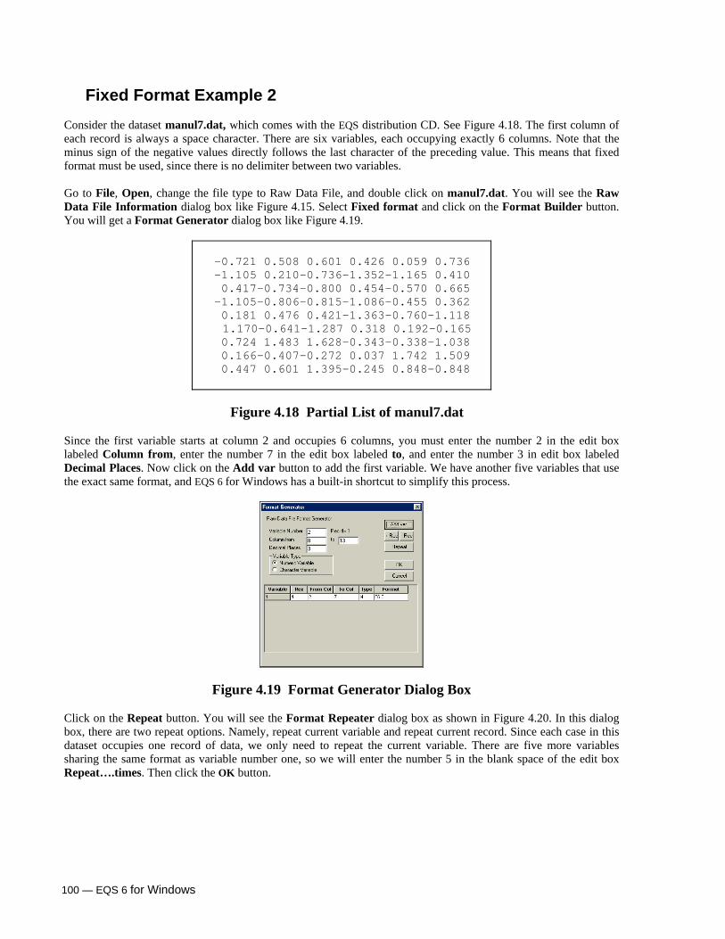
100 — EQS 6 for Windows
Fixed Format Example 2
Consider the dataset manul7.dat, which comes with the EQS distribution CD. See Figure 4.18. The first column of each record is always a space character. There are six variables, each occupying exactly 6 columns. Note that the minus sign of the negative values directly follows the last character of the preceding value. This means that fixed format must be used, since there is no delimiter between two variables. Go to File, Open, change the file type to Raw Data File, and double click on manul7.dat. You will see the Raw Data File Information dialog box like Figure 4.15. Select Fixed format and click on the Format Builder button. You will get a Format Generator dialog box like Figure 4.19.
-0.721 0.508 0.601 0.426 0.059 0.736 -1.105 0.210-0.736-1.352-1.165 0.410 0.417-0.734-0.800 0.454-0.570 0.665 -1.105-0.806-0.815-1.086-0.455 0.362 0.181 0.476 0.421-1.363-0.760-1.118
1.170-0.641-1.287 0.318 0.192-0.165 0.724 1.483 1.628-0.343-0.338-1.038 0.166-0.407-0.272 0.037 1.742 1.509 0.447 0.601 1.395-0.245 0.848-0.848
Figure 4.18 Partial List of manul7.dat
Since the first variable starts at column 2 and occupies 6 columns, you must enter the number 2 in the edit box labeled Column from, enter the number 7 in the edit box labeled to, and enter the number 3 in edit box labeled Decimal Places. Now click on the Add var button to add the first variable. We have another five variables that use the exact same format, and EQS 6 for Windows has a built-in shortcut to simplify this process.
Figure 4.19 Format Generator Dialog Box Click on the Repeat button. You will see the Format Repeater dialog box as shown in Figure 4.20. In this dialog box, there are two repeat options. Namely, repeat current variable and repeat current record. Since each case in this dataset occupies one record of data, we only need to repeat the current variable. There are five more variables sharing the same format as variable number one, so we will enter the number 5 in the blank space of the edit box Repeat….times. Then click the OK button.

EQS 6 for Windows — 101
Figure 4.20 Format Repeater You will see the Format Repeater dialog box is closed and the formats of all six variables are displayed in the Format Generator dialog box (Figure 4.21). Click the OK button to return to return to Raw Data Information Dialog Box and click on OK again. The dataset will be opened as shown in Figure 4.22.
Figure 4.21 Format Generator
Figure 4.22 Imported Fixed Format Data
Options in Format Generator
Format generator is a general and convenient tool to import fixed format data. When you are specifying the format, mistakes may be made, but you don’t have to abandon all the work you have done. Or, if the dataset you have imported is not properly saved, you may have to import it again. You don’t have to re-specify the format, which may be time consuming if the formats of variables are irregular. We will show you how to edit the formats that have been specified.
Reload previously specified format
After successfully importing the fixed format data file test.dat, close the file and reopen it again. Select the File menu Open option and choose test.dat. When you see the Raw Data File Information dialog box, click on the radio button labeled Fixed format, then click on the Format Builder button. You see a dialog box as shown in Figure 4.23.
Figure 4.23 File Format Reload Dialog Box

102 — EQS 6 for Windows
Press YES; you will see the Format Generator dialog box open with the previously specified format filled in (Figure 4.24).
Figure 4.24 Format Generator Dialog Box This convenient option allows you to retain the format information of a data file should you need to import this data file again. Or, if you have made a mistake on the format you have specified, it allows you to modify the format without redoing everything from scratch.
Note: Please note that EQS can only remember the format specification for the most recently opened file. You cannot trace back to a file that is not the most recently opened one.
Editing and deleting the format The variable formats specified in the can be modified. You can delete the last format line in the Format Generator variable format list box by double clicking on it. In contrast, double clicking on any other line in the list box has a different effect. You can double click on any line other than the bottom line to bring up an editing dialog box for that line. To edit variable 1 in record 1, double click on the variable 1 format line in the list box. The Format Editor dialog box will appear (Figure 4.25).
Figure 4.25 Format Editor Dialog Box Change the Ending column to 4 and the Decimal places to 1. Click on OK, and you will see the message box shown in Figure 4.26.

EQS 6 for Windows — 103
Figure 4.26 Editing Message Figure 4.27 Modified Format Generator Since you have changed the Ending column for variable 1 from 3 to 4, variable 1 could extend into the space reserved for variable 2 (although in this case, it does not). Thus, the program prompts you to decide whether to move all succeeding variables one column to the right should the variable formats conflict with each other. You should click on YES to avoid conflicts between variables. After you click YES, you will return to the Format Generator dialog box and the format of variable 1 will be changed accordingly (Figure 4.27). In this example, the change to variable 1 will not affect the subsequent variables since the second variable starts at column 5. If, however, the second variable started at column 4, you would see changes to the format of that variable, and possibly others.
Repeat Option We will use manul7.dat again to illustrate another way to use the Repeat option in the Format Generator. Let’s open it as described just before Figure 4.18. This dataset has 6 variables and 50 cases, but let’s pretend it has 12 variables with a sample size of 25. Thus, each case takes two lines of data. Go to File, select Open, change the file type to Raw data file, and select manul7.dat. In the Raw Data File Information Dialog Box, click on the Format Builder button. The Repeat option allows you to repeat the format for the last specified variable one or more times. This option is valuable when you have several variables with the same format. Let’s specify the format of the first variable. As we did above, we enter the number 2 into the edit box labeled Column from, enter the number 7 into the edit box labeled to, and enter the number 3 into the edit box labeled Decimal Places. The entries are shown in Figure 4.28. Now we could press Add var, then use the Format Repeater to repeat the format five times, as we did above (see Figure 4.19). Instead, click immediately on the Repeat button to bring up the Format Repeater dialog box, and enter 6 in the Repeat….times box (Figure 4.29).
Figure 4.28 Format Generator
Figure 4.29 Format Repeater

104 — EQS 6 for Windows
Repeat Current Variable Click OK, and the Format Generator dialog box will display 6 defined variables (Figure 4.30).
Figure 4.30 Format Generator Dialog Box with Variable Repetitions
Repeat Current Record Now we use the Repeat option to duplicate the current record. Click on the Repeat option in the Format Generator dialog box. When you see the Repeat option dialog box (Figure 4.31), click to choose Current record. Enter 1 in the Repeat….times field. Click OK to finish and return to the Format Generator dialog box (Figure 4.32).
Figure 4.31 Format Repeater
Figure 4.32 Format Generator Dialog Box
You can see that the second record is now filled in (Figure 4.32), and is identical to the first. When all the formats are specified, click the OK button to return to previous dialog box and click OK again. The data file will be opened (Figure 4.33). In this case, the EQS Data Editor contains a file of 12 variables with a sample size of 25.
Figure 4.33 Fake Example for manul7.dat

EQS 6 for Windows — 105
Specifying a New Record If your file had more than one record per case, you could use the Format Generator dialog box to define the format for those additional records. Just click on the +Rec button to toggle up through other possible record numbers. Click three times on the +Rec button, and you will see the Rec# = field change from 1 to 4 in the Format Generator dialog box. Click twice on the -Rec button to move back down to Rec# = 2.
Figure 4.34 Format Generator Set for Record #2 Note that the Format Generator dialog box displays Column from 1 to 1 for Record# = 2 after you press the +Rec button. Now that you have chosen a different record, you can enter the specifications for this record. For our example, we will enter the number 2 for the beginning column and number 7 as the ending column with a decimal place of 3. Click on the Add var button when you finish the specifications for each variable in record 2 or use format repeater as you wish. Click on OK when you have finished specifying the records for the data file.
Saving and Exporting Data and Other Files Whenever you choose the Save As dialog box from the File option in the main menu, you will be saving the file in one of two formats. These are: Text Files and EQS System Files. EQS model files with the *.eqs extension are saved as Text Files. Text files are document files that contain characters and numbers. In principle, they are readable by any editor or word processor that permits the importing of plain ASCII or text files. EQS system data files with the *.ess extension are saved as EQS System Files. As System Files, they are saved in a special format that maintains information about the dataset itself, such as number of cases and variables, and labels for the variables. These files can be read quickly by the EQS program, but are meaningless to other computer programs. Thus, if you want to save a data file for export to another statistical package, you must save the file as a text file, not an EQS system file. When creating a text file with EQS, the file name that you use does not matter. For example, you could save it as a *.dat or a *.txt file. We strongly urge you to save the data file with *.dat extension. However you save the file, the file type designation should correspond to its intended use.

106 — EQS 6 for Windows
EQS 6 for Windows provides two ways to save your text files, as you can see in Table 4.2.
Text File Type Text File Delimiter Recommended Usage Data File space-delimited and wrapped at 80 columns files for mainframe and Email w/ Tab Delimiter tab-delimited without wrapping files for MS Excel, SPSS, etc.
Table 4.2 Delimiters for Saving Text Files in EQS
To create text data files in EQS 6 for Windows, use the File menu Save As option and choose your preferred text file type. Figure 4.35 shows the two text file types in the Save File as Type list.
Figure 4.35 Save As Dialog Box with Text File Types
You must choose from text data file or tab delimited data file and enter the file name is the file name field. Click the Save button when you are done. The data file will be saved into a text file using either space or a tab character as its delimiter.
Saving SPSS System Files You can also save an EQS data sheet as an SPSS *.sav file. For those of you who use SPSS for Windows as your data analysis tool, you know what SPSS *.sav files are. An SPSS *.sav file is an SPSS dataset in machine language binary format. It contains information such as variable names, value labels, various missing data information, the file directory, etc. Sometimes it also contains a transformation syntax. The ability to save an EQS data sheet into an SPSS *.sav file gives you the option to use SPSS to analyze information produced by EQS 6. For example, EQS can impute missing data using its EM methodology, and add factor scores, regression estimates and residuals, etc. to your data file. Then, you can export such newly created information to SPSS for further analysis. To save an EQS 6 data sheet into an SPSS file, uses File Save As SPSS System File (from Save as type) and provide an appropriate name for your SPSS dataset (Figure 4.36).

EQS 6 for Windows — 107
5. PLOTS A data plot helps you to efficiently present your data. The data plot not only presents your data in an organized way, but also gives you a clearer impression of the data than you can get from the raw numbers. EQS 6 for Windows provides many types of data plots that you can use to present and diagnose your data. In this chapter, we discuss how to access the plot functions in EQS 6 for Windows. You call up the plots through the plot icons located under the Window menu bar.
Figure 5.1 EQS 6 for Windows Plot Icon Tools Figure 5.1 shows all of the plot icon tools. These plot icons represent (from left to right):
1. Line Plot 2. Area Plot 3. Histogram 4. Pie Chart 5. Bar Chart 6. Quantile Plot 7. Quantile-Quantile Plot 8. Normal Probability Plot 9. Scatter Plot (including Matrix Plot) 10. Surface Plot (3D function plot) 11. Box Plot 12. Error Bar Chart
Start a Plot As discussed in previous chapters, EQS 6 for Windows is a data-oriented program. It functions only with a proper data file (i.e., *.ess file) in the Data Editor. To work with the plot functions, go through the following steps: Step 1: Open a Data File Step 2: Select a Plot Icon Step 3: Specify Variable(s) and Options in the Plot dialog box Step 4: Activate the Plot Step 5: Save the Plot
Step 1: Open a Data File
The procedure for opening a data file was discussed in great detail in Chapter 3, and will not be repeated here. The data file used for plotting must be a raw data file, not a covariance or correlation file.

108 — EQS 6 for Windows
Step 2: Select a Plot Icon
Let’s assume that you have opened the airpoll.ess data file that came with the EQS 6 for Windows program CD. To create a scatter plot, you select the scatter plot icon from the Plot Icon list (as shown in Figure 5.1). In fact, the scatter plot icon looks like a scatter plot. Click on the icon once to select it.
Step 3: Specify Variable(s) and Options in Plot Dialog Box
After you select the scatter plot icon, the Scatter Plot dialog box will appear (Figure 5.2).
Figure 5.2 Scatter Plot Dialog Box The dialog box contains four list boxes. The left list box labeled Variable list contains all the variables in the dataset. The top right list box is labeled Y axis, while the list box below it is labeled X axis. You can select (highlight) one or more variables from the Variable list and move them to the Y axis. Similarly, you move variable(s) to the X axis. When the list boxes for both axes have one or more variables in them, the list box labeled Grouping variable becomes active, allowing you to specify an optional grouping variable for the plot. By default, the scatter plot is displayed without a grouping variable. For this example, click on NONWHITE and move it to the Y axis box, then click on EDUCATN and move it to the X axis box. After you have prepared the two variables, you have completed all specifications needed for a scatter plot.
Step 4: Activate the Plot
The bottom of the dialog box contains two buttons. Press the OK button to actually create the scatter plot. (You would press the Cancel button to return to your dataset without taking any action.) A new window titled Scatter Plot is displayed (Figure 5.3). There is a horizontal toolbar situated under the window title, followed by a strip of color palettes. You can change the color of the plot symbol or plot window by dragging a selected color to that symbol or window. At the right side of the plot window, you will see the bivariate regression equation and its R square.

EQS 6 for Windows — 109
Figure 5.3 Scatter Plot Display
As you can see in Figure 5.3, there is a tool icon located in the upper left corner of the plot window. This black hole tool icon is unique to a scatter plot. You can select one or more data points from your scatter plot and drag these points to the black hole. Once data points are dropped from the scatter plot window into the black hole, these points are removed from the plot window and the bivariate regression is recomputed. When there are data points in the black hole, these points are highlighted in black in your Data Editor. It is a very good tool to identify outliers visually. You can see from this example that you can create a presentation quality plot with only a few clicks. A high quality plot will help you present the results of your analysis to your audience.
Step 5: Save the Plot
See the sections Save and Copy Graphic to Clipboard at page 135. In the following section, we assume that you already know how to bring a file to the Data Editor. Each plot example specifies a data file appropriate for the example. Please bring the specified file into the Data Editor before continuing with the plot example.
Line Plot A Line Plot plots the score of a variable on the vertical axis and the sequence of the score on the horizontal axis. Since it plots the case sequence of a variable, a line plot is useful for viewing the trend of the variable across the data points (e.g., data collected at different times). The Line Plot in EQS 6 for Windows allows you to plot up to 12 variables on the same plot. If your cases are not in order, you may want to use the Sort option described in Chapter 3 before creating a line plot.

110 — EQS 6 for Windows
Let’s look at the data in furnace.ess installed from the EQS 6 for Windows CD. Furnace.ess comes from Box and Jenkins5. The data consist of two variables, GAS and CO2. GAS is the input and CO2 is the output of an industrial process. Let’s try to plot GAS on a line plot.
Specifying Variables Click on the line plot icon (see Figure 5.1) to start the plot. The Line Plot dialog box will appear (Figure 5.4).
Figure 5.4 Line Plot Dialog Box In the dialog box there are two variables, GAS and CO2. Click on GAS to select it and using the right arrow button to move GAS to the Variables to Plot box. Click the OK button to plot.
Display Line Plot As soon as you click the OK button, the line plot will appear (Figure 5.5). You can see from the plot that the Y-axis is the GAS variable and the label is printed in landscape mode. The X-axis just shows the sequence of the data. Note that there is a line drawn across the plot frame at the variable mean.
Figure 5.5 Line Plot Display
5 Box, G. E. P. and G. M. Jenkins (1976). Time Series Analysis: Forecasting and Control. San Francisco: Holden Day.

EQS 6 for Windows — 111
The plot in Figure 5.5 shows regular fluctuation over the data-collecting period. If you want to see more than one variable on the same plot, use the Line Plot dialog box shown in Figure 5.4 to select up to 12 variables for each line plot. When drawing multiple variables, the program uses the minimum and the maximum of the specified variables as the range of the Y-axis. Since all variables use the same scale, the line plot lets you see the differences between variables. Variable mean lines, however, do not appear in a multiple variable line plot.
Area Plot
An Area Plot plots the score of a variable on the vertical axis and the sequence of the score on the horizontal axis with the area under the curve filled in. Since it plots the case sequence of a variable and emphasizes the area under the curve, an area plot is useful for viewing the trend of the variable across the data points. If your cases are not in order, you may want to use the Sort option described in Chapter 3 before creating an area plot. The Area Plot in EQS 6 for Windows allows you to plot up to four variables on the same plot. For each successive variable, the program uses the plot for the previous variable as the base. EQS plots the variables in their order in the variable list. Thus, you may find it helpful to use the Cut and Paste options to rearrange your variables for an informative area plot. Let’s look at the data in exercise.ess. The exercise.ess dataset comes from the BMDP Statistical Software Manual, Volume 16. The original data file contains eight variables. The last two variables are non-numeric variables, which are not acceptable to EQS 6 for Windows. Thus, for EQS 6 for Windows, exercise.ess contains only six variables. This dataset measures pulse rate for 40 subjects before and after running one mile. We use PULSE_1 to represent the pulse rate before running and PULSE _2 for pulse after running. Let’s try to plot exercise.ess on an area plot.
Specifying Variables
Select the Area Plot icon (see Figure 5.1) to start the plot. The Area Plot dialog box will appear (Figure 5.6).
Figure 5.6 Area Plot Dialog Box
In the dialog box, click on two variables, PULSE_1 and PULSE_2 and move them to the box labeled Variables to Plot. Click the OK button to plot.
6 Dixon, W. J. (1993). BMDP Statistical Software Manual. Berkeley, CA: University of California Press.
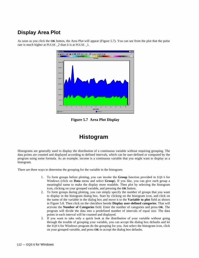
112 — EQS 6 for Windows
Display Area Plot
As soon as you click the OK button, the Area Plot will appear (Figure 5.7). You can see from the plot that the pulse rate is much higher at PULSE _2 than it is at PULSE _1.
Figure 5.7 Area Plot Display
Histogram Histograms are generally used to display the distribution of a continuous variable without requiring grouping. The data points are counted and displayed according to defined intervals, which can be user-defined or computed by the program using some formula. As an example, income is a continuous variable that you might want to display as a histogram. There are three ways to determine the grouping for the variable in the histogram:
1. To form groups before plotting, you can invoke the Group function provided in EQS 6 for Windows (click on Data menu and select Group). If you like, you can give each group a meaningful name to make the display more readable. Then plot by selecting the histogram icon, clicking on your grouped variable, and pressing the OK button.
2. To form groups during plotting, you can simply specify the number of groups that you want to display in the histogram dialog box. Start by clicking on the histogram icon, and click on the name of the variable in the dialog box and move it to the Variable to plot field as shown in Figure 5.8. Then click on the checkbox beside Display user-defined categories. That will activate the Number of Categories field. Enter the number of categories and press OK. The program will divide the data into a predefined number of intervals of equal size. The data points in each interval will be counted and displayed.
3. If you want to take only a quick look at the distribution of your variable without going through the trouble of grouping your variable, you can accept the dialog box defaults and let the EQS 6 for Windows program do the grouping for you. Just select the histogram icon, click on your grouped variable, and press OK to accept the dialog box defaults.
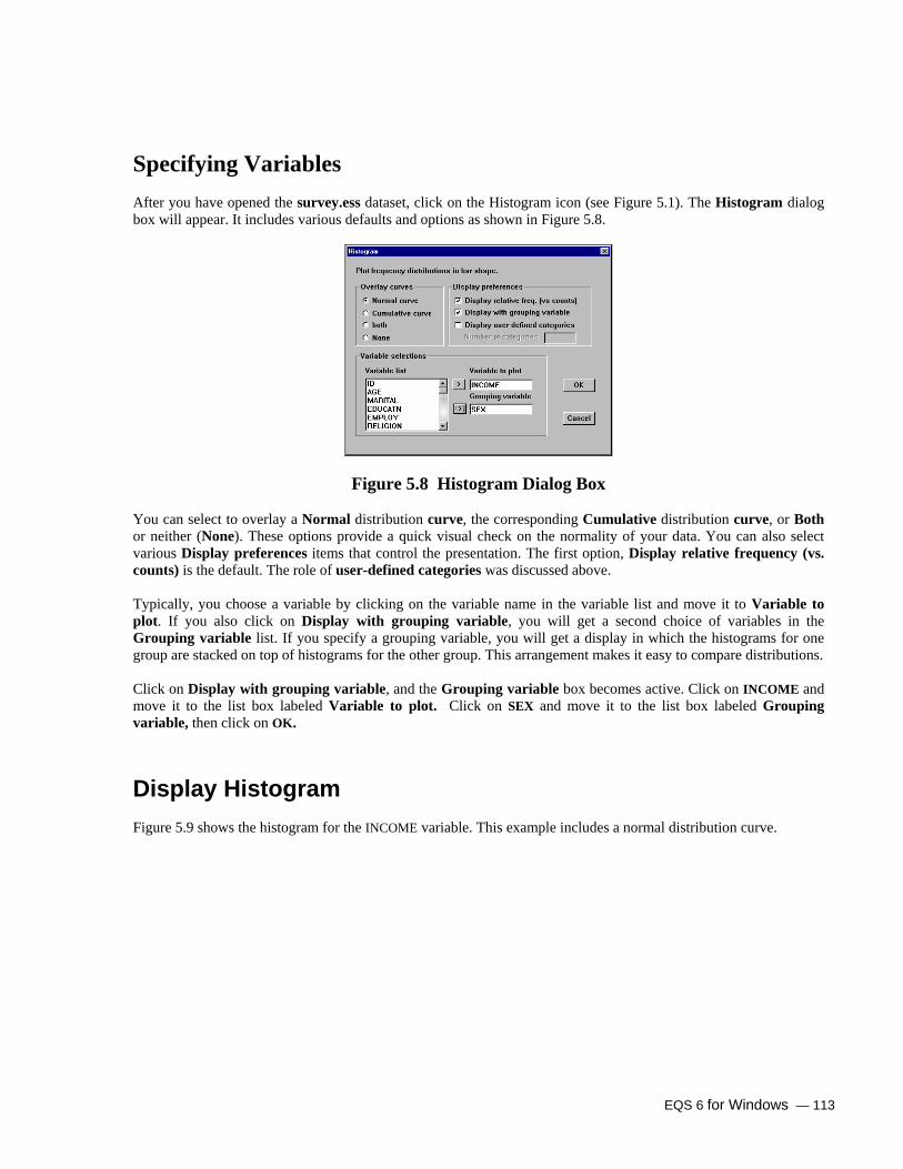
EQS 6 for Windows — 113
Specifying Variables After you have opened the survey.ess dataset, click on the Histogram icon (see Figure 5.1). The Histogram dialog box will appear. It includes various defaults and options as shown in Figure 5.8.
Figure 5.8 Histogram Dialog Box
You can select to overlay a Normal distribution curve, the corresponding Cumulative distribution curve, or Both or neither (None). These options provide a quick visual check on the normality of your data. You can also select various Display preferences items that control the presentation. The first option, Display relative frequency (vs. counts) is the default. The role of user-defined categories was discussed above. Typically, you choose a variable by clicking on the variable name in the variable list and move it to Variable to plot. If you also click on Display with grouping variable, you will get a second choice of variables in the Grouping variable list. If you specify a grouping variable, you will get a display in which the histograms for one group are stacked on top of histograms for the other group. This arrangement makes it easy to compare distributions. Click on Display with grouping variable, and the Grouping variable box becomes active. Click on INCOME and move it to the list box labeled Variable to plot. Click on SEX and move it to the list box labeled Grouping variable, then click on OK.
Display Histogram Figure 5.9 shows the histogram for the INCOME variable. This example includes a normal distribution curve.

114 — EQS 6 for Windows
Figure 5.9 Histogram Display Note: If you choose to overlay a normal distribution curve on a histogram to see whether the scores are
normally distributed, it is important that none of the ordered categories are missing.
Pie Chart The pie chart, or pie graph, is an alternative way of displaying a categorical variable. Unlike the histogram, the pie graph focuses on the proportion for each category. Again, we will use survey data to see the levels of education.
Specifying Variables Open the data file survey.ess in the Data Editor, and then select the pie chart icon (see Figure 5.1). A pie chart variable selection dialog box will appear (Figure 5.10). Within the dialog box, select the EDUCATN variable and click the OK button.
Figure 5.10 Pie Chart Dialog Box
Display Pie Chart
After you click on OK, a new window appears, displaying a pie chart (Figure 5.11). Each category in the pie is distinguished by a different color. The size of each slice represents the proportion of that category to total sample
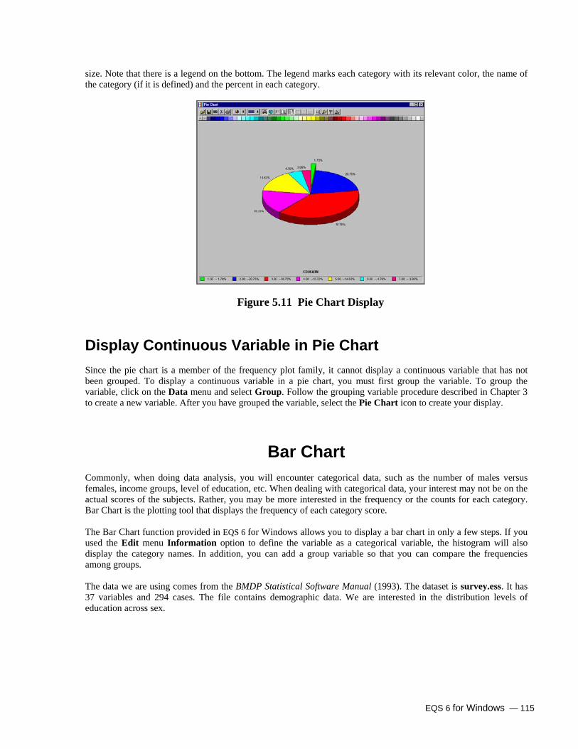
EQS 6 for Windows — 115
size. Note that there is a legend on the bottom. The legend marks each category with its relevant color, the name of the category (if it is defined) and the percent in each category.
Figure 5.11 Pie Chart Display
Display Continuous Variable in Pie Chart
Since the pie chart is a member of the frequency plot family, it cannot display a continuous variable that has not been grouped. To display a continuous variable in a pie chart, you must first group the variable. To group the variable, click on the Data menu and select Group. Follow the grouping variable procedure described in Chapter 3 to create a new variable. After you have grouped the variable, select the Pie Chart icon to create your display.
Bar Chart Commonly, when doing data analysis, you will encounter categorical data, such as the number of males versus females, income groups, level of education, etc. When dealing with categorical data, your interest may not be on the actual scores of the subjects. Rather, you may be more interested in the frequency or the counts for each category. Bar Chart is the plotting tool that displays the frequency of each category score. The Bar Chart function provided in EQS 6 for Windows allows you to display a bar chart in only a few steps. If you used the Edit menu Information option to define the variable as a categorical variable, the histogram will also display the category names. In addition, you can add a group variable so that you can compare the frequencies among groups. The data we are using comes from the BMDP Statistical Software Manual (1993). The dataset is survey.ess. It has 37 variables and 294 cases. The file contains demographic data. We are interested in the distribution levels of education across sex.

116 — EQS 6 for Windows
Specifying Variables To start a bar chart, open survey.ess. Then select the plot icon representing the bar chart (see Figure 5.1). After you click on the icon, the Bar Chart dialog box will appear (Figure 5.12).
Figure 5.12 Bar Chart Dialog Box
This box provides you with choices in Display style (Standard, the default; Stacked, one on top of the other; Parallel, two side by side) and various options in Display preferences. Preferences include Display vertical bars, use of Real scores (vs. percentile), and plotting in 2-D or 3-D. The 2-D option, Plain display, is the default. Finally, to see the level of one variable grouped by another, you can choose Grouping variable.
Display Bar Chart
As an example, to view the bar chart of education by sex, check the checkbox labeled Display with grouping variable. The list box labeled Grouping variable becomes active. Move the variable SEX as the Grouping variable and select EDUCATN from the Variable list and move it into Variable to plot field. Click the OK button to display the plot.
Figure 5.13 Stacked Bar Chart
Figure 5.13 shows the bar chart for the EDUCATN variable grouped by SEX. The plot displays seven categories of EDUCATN. Each bar contains two parts. The upper blocks are female, while the lower blocks are male. The Y-axis

EQS 6 for Windows — 117
shows the frequency of each education level. The X-axis shows the code for each category. If you defined the EDUCATN variable as categorical and specified each category with a code name, the code names will replace codes on the X-axis.
Quantile Plot The Quantile plot is a tool to help you assess the distribution of your data. It plots the ordered data on the Y-axis and the fraction of the data on the X-axis. The formula for calculating the fraction of the data is in the BMDP Statistical Software Manual Volume 1 or a statistics book such as Hamilton7.
Specifying Variables To illustrate the Quantile Plot we use the survey.ess INCOME variable. To start the plot, click on the Quantile plot icon (see Figure 5.1). A Quantile Plot variable selection dialog box will appear (Figure 5.14). Select the INCOME variable and click the OK button.
Figure 5.14 Quantile Plot Dialog Box
Display Quantile Plot
The quantile plot display is shown in Figure 5.15. The Y-axis provides the data scores sorted in ascending order, and the X-axis gives the fraction of the data. The fraction is calculated at (i-0.5)/n, where i is the sequence of the data point and n is the sample size. If the data are normally distributed, the plot will be bow-shaped. If the points lie on the diagonal line, the data are uniformly distributed. For a detailed discussion of the Quantile plot, refer to any standard textbook.
7 Hamilton, L. C. (1992). Regression with Graphics—A Second Course in Applied Statistics. Pacific Grove, California: Brook/Cole Publishing Co.

118 — EQS 6 for Windows
Figure 5.15 Quantile Plot Display
Quantile-Quantile Plot Quantile-Quantile plots are sometimes called QQ plots. A QQ plot will plot the quantiles of one variable against the quantiles of another variable. Thus, it sorts two variables, both in ascending order, plotting one variable on the Y-axis, the other variable on the X-axis. The QQ plot allows you to compare two observed variables. (To plot one observed variable against a known distribution, see Normal Probability Plots, below.) To illustrate this plot, again we use a dataset called exercise.ess.
Specifying Variables Click on the QQ icon (see Figure 5.1). A dialog box will appear, allowing you to specify variables (Figure 5.16).
Figure 5.16 Quantile-Quantile Plot Dialog Box Unlike the frequency plots (i.e., histogram, pie chart, etc.), you must specify exactly two variables in the list box labeled Variables to Plot, one variable for each axis. In this illustration we are interested in the PULSE_1 and PULSE _2 variables. You can select variables PULSE _1 and PULSE _2 and move them into the list box labeled Variables to Plot, click the OK button to activate the plot.

EQS 6 for Windows — 119
Display QQ Plot
The resulting QQ plot is shown in Figure 5.17. The dot pattern of the QQ plot shows that the distributions of these two variables are quite different. If the distributions of the two variables were identical, they would form a straight line along the diagonal line of the plot. The current dot pattern appears to be close to a straight line with the exception of one case. The offset from the diagonal suggests that the two variables may have a similar distribution pattern, but with different means. The case in the upper right corner may be an outlier. More discussions on the shape of the dot pattern and its meaning can be found, for example, in Hamilton’s text.
Figure 5.17 Quantile-Quantile Plot Display
Normal Probability Plots Normal Probability plots are also known as Quantile-Normal or Normal-Quantile plots. They are a variation of the QQ plot. Note that the QQ plot graphs two sorted variables to compare the distributions. If you replace the Y-axis by a known distribution, say a normal distribution, you are actually comparing the distribution of a variable against the normal distribution. To compute the Y-axis, we take the expected normal value from the rank of an observed variable against the actual variable sorted in ascending order. You can find a detailed description of expected standard normal value in the BMDP Statistical Software Manual or any standard statistical textbook. Since we are plotting the expected standard normal value against an observed variable, a straight line lying on the 45 degree diagonal means that the distribution of the data is perfectly normal. The distribution of the observed variable is implied in the dot patterns of the plot. Hamilton’s text, cited above, has an extensive discussion of the various possible patterns. Use exercise.ess as the test dataset illustrating the normal probability plot. The variable is PULSE_1.
Specifying Variables Click on the Normal Probability plot icon (see Figure 5.1) to get the Normal Probability Plot dialog box (Figure 5.18). Then select the PULSE _1 variable from the list box in the figure and move it into the list box labeled Variable to Plot. Click on the OK button when you are ready to plot.

120 — EQS 6 for Windows
Figure 5.18 Normal Probability Plot Dialog Box
Display Normal Probability Plot
The normal probability plot is shown in Figure 5.19. The dot pattern shows that the PULSE_1 variable is not perfectly normally distributed. The observed variable does not skew, because the dot pattern crosses the Y-axis at about 0.0. The dot pattern shows that both tails are long and flat.
Figure 5.19 Normal Probability Plot Display
Scatter Plots The scatter plot is one of the most widely used statistical plots. It plots two variables against each other to examine the scatter of the observations. You can select up to 12 variables for each axis. The scatter plot is a good tool for displaying the relationship between variables, evaluating their linear relation, and detecting outliers. The beginning of this chapter has an example of the scatter plot in EQS 6 for Windows (Figure 5.3). The scatter plot option displays the plot, draws the bivariate linear regression line, and prints the regression equation and its R square. Besides the features mentioned above, the scatter plot option in EQS 6 for Windows displays matrix plots (more than one variable on each axis), supports brushing (encircling a few data points in one plot causes the same data points to be highlighted in other plots), zooming, temporary removal of outliers, and marking outliers in the Data Editor. These features dynamically link your data and your plot. You can use the scatter plot not only to show the plots, but also use the plot to diagnose outliers.

EQS 6 for Windows — 121
To demonstrate the scatter plot, we use fisher.ess from the BMDP Statistical Software Manual. The dataset contains sepal length and width and petal length and width for three species of iris. Since we showed the single scatter plot earlier, this example will demonstrate a matrix plot with three variables on both X- and Y-axes.
Specifying Variables Click on the Scatter Plot icon (see Figure 5.1) to get the Scatter Plot dialog box (Figure 5.20).
Figure 5.20 Scatter Plot Dialog Box For a detailed explanation of the list boxes in the dialog box, see the paragraph below Figure 5.2. In this example, let’s select the first three variables from the variable list and move them to both Y-axis and X-axis list box. Please note that both Y-axis and X-axis can share the same variable. Click on the OK button. The scatter plot will appear.
Display Scatter Plots
Figure 5.21 shows the 3 by 3 matrix plot. Note that you have selected the same variables on the X- and Y-axes. Thus, the diagonal plots in the matrix would be scatter plots of one variable against itself, resulting in a straight line. Rather than display the straight line, EQS 6 for Windows displays the histogram of the variable.
Notice that several of the scatter plots show points that are grouped together, with some blank spaces. Evidently, the scores cluster to form groups.

122 — EQS 6 for Windows
Figure 5.21 Matrix of Scatter Plots
Brushing Brushing is a technique that has been frequently used in recent years. Brushing is generally applied in the matrix plot, but is also useful in a single scatter plot. In a matrix plot, you might be interested in certain data points in one cell and want to know where those cases are in another cell of the matrix plot. The brushing technique allows you to encircle a group of points in one cell by creating a rectangle defined by a broken line. The color of the enclosed data points will change, and that color will be picked up by the same cases in the other cells. Moreover, you can drag the designated rectangle to another position in the cell, highlighting any data points that are enclosed. This is a useful feature to identify a few data points that are unique and require more attention. To create a brushing effect in EQS 6 for Windows, place your mouse pointer in one cell and drag a rectangle from the upper left to the lower right. After you release the mouse button, the rectangle will stay and all data points within the rectangle will turn red. We call the rectangle a brush. The brush must enclose one or more data points, or it will disappear. Once you have created the brush, you can drag the brush anywhere in the cell. To remove the brush, draw the brush without including any data points within the rectangle. The brush and the marked data points will disappear.
Zooming When you have a matrix of plots on the screen, you may want to investigate one cell more closely, or determine the R square for a particular cell. EQS 6 for Windows provides a solution. You can blow up any cell in a matrix plot by zooming. To zoom a cell, double click anywhere within the boundary of the cell that you want to zoom. The matrix plot will be replaced by a single scatter plot with the regression line and the R square. To return to the matrix plot, double click on any point within the zoomed plot.

EQS 6 for Windows — 123
Outlier Detection and Diagnosis Outlier detection is a unique feature of EQS 6 for Windows. It provides a convenient way to display outliers and temporarily remove suspicious data points without recomputing the plot or changing the data file. Open the dataset manul7.ess. This dataset is simulated data with 50 cases, and case 50 is an outlier case. Let’s create a scatter plot between variable V1 and variable V4 where the V1 is on the Y-axis and variable V4 is on the X-axis. The scatter plot is shown in Figure 5.22. Note the dot on the upper right corner, far from the cluster of data in the lower left corner. The plot provides the bivariate regression information as usual. If you want to see the R square without this outlier, you can temporarily remove that outlier by dumping the point in the black hole. The black hole is the icon located on the upper left corner of the scatter plot. As you can imagine, it looks like a black hole in a science fiction movie. It is a place for temporary storage of undesirable data points. To use the black hole storage, create a brush to mark the undesirable data point. Once it is marked, drag the entire brush into the black hole. The size of the brush does not matter, as long as the mouse pointer lies directly over the black hole when you release the mouse button. After you release your mouse button, a dot appears in the center of the black hole. That dot is a reminder that you have something in the black hole. After you dump one or more data points into the black hole, the plot information will be recalculated. Therefore, you can see the slope of the regression line, the confidence interval lines, and the R square change (see Figure 5.23). You can repeatedly put data points in the black hole. To recover the data points from the black hole, just double click on the black hole.
Note: Do not put all data points into the black hole, because that may generate unpredictable results.
Figures 5.22 Scatter Plot with Outlier Figure 5.23 Scatter Plot without Outlier
Mark Selected Data Points in Data Editor Since you can examine the potential outliers from the scatter plot by dumping cases in and out of the black hole, it would be nice to mark those outlying cases in the Data Editor so that you can exclude them from further analysis. EQS 6 for Windows allows you to mark cases in the Data Editor. To do so, follow these steps:

124 — EQS 6 for Windows
Step 1: Put outlying cases in the black hole The black hole is the bridge between the scatter plot and the Data Editor. Therefore, move cases to be marked into the black hole. If you followed the scatter plot example above, you already have one case in the black hole.
Step 2: Mark points in data sheet The data point(s) not in the black hole will be automatically marked in the Data Editor.
Step 3. Verify the marked cases or reverse selection
After you have marked a case in the Data Editor, you can verify your action by clicking Data and selecting Information. An informational dialog box will appear, indicating the number of cases marked. If you then perform an analysis, that analysis will be performed on the marked cases.
Figure 5.24 Data File Information after Marking
You may find it necessary to reverse the marking selection! In Figure 5.24, for example, you may be interested in the one outlier case that is not marked. In such a situation, you can go to the main menu, select Data and Use Data. Then you get the Case Selection Specification dialog box, where you check Reverse Selection/Unselection of Cases. This marks the one outlier case. If you are creative in applying these dynamic features, along with the data handling capabilities, you can fully explore your data. EQS 6 for Windows can take you to a new level of data analysis.
Surface Plot A Surface Plot or 3D Function Plot is a useful tool to examine a user-defined mathematical function. It does not require any data. The EQS plot program will compute all necessary data if you provide the range of both X- and Y-axes and the function you want to plot. The function plot will divide the range of X- and Y-axes into many small intervals, and compute the height of the Z-axis according to the function. It then plots the user-defined function on a three-dimensional surface. The height of the Z-axis and its contours are shown in various colors.
Specifying Plotting Range

EQS 6 for Windows — 125
Click the Surface Plot icon (see Figure 5.1) to start the plot. The Surface Plot dialog box appears.
Figure 5.25 Surface Plot Dialog Box
The dialog box has been divided into three parts. (1) the Start value and End value of X axis, (2) the Start value and End value of Y Axis, and (3) the function you want to plot. In our example, the range of X axis is between 5 and 10. The range of Y Axis is between -5 and 5. The function is
Z = X**2 * SIN(X)*COS(Y)
You only need to enter the right hand side of the function. Please make sure that all letters are upper case (Figure 5.25).
Display Surface Plot
After filling all required information in the dialog as shown in Figure 5.25, click the OK button. The plot will be shown as Figure 5.26.
Figure 5.26 Surface Plot Display

126 — EQS 6 for Windows
Box Plot The box plot only plots summarized information. It is widely used for viewing the distribution of data and the possible outliers. This is in contrast to Quantile and QQ plots which show the raw scores. The plot consists of three parts: the body, the tail, and the outliers. The body part is actually the box itself. The top of the box is the third quartile or Q3 (75% of the cases will fall below this line and 25% of the cases will fall above this line). The bottom of the box is the first quartile, or Q1. The range between the top and the bottom of the box is called the inter-quartile range or IQR. There is an upper tail above the box at the position of Q3+1.5IQR, or the maximum of the data, whichever is smaller. There is also a lower tail at the position of Q1-1.5IQR, or the minimum of the data, whichever is larger. The data points that fall beyond the upper or lower tails will be plotted in their real position. The median is also shown.
Specifying Variables
We use manul7.ess to illustrate the box plot. With that file open, click on the box plot icon (see Figure 5.1) to get the Box Plot dialog box. When selecting multiple variables, be sure to choose variables with similar ranges. Otherwise, the different ranges may make the plot unreadable, because EQS 6 for Windows uses the range of values for the first variable to define the axis. Choose the first three variables and click OK to display the box plot.
Figure 5.27 Box Plot Dialog Box
Display Box Plot The box plot display is shown in Figure 5.28. It plots three variables side by side. You can see that there are outliers in the plot; they appear in a contrasting color on a color monitor. Near the center of each box, there is a horizontal line that represents the median of the variable.

EQS 6 for Windows — 127
Figure 5.28 Box Plot Display
Error Bar Chart The error bar chart plots summarized information for several variables. It consists of the mean and the error bars for each variable. The means are connected by a line.
Specifying Variables
We use manul7.ess to illustrate the error bar plot. With that file open, click the Error Bar chart icon (see Figure 5.1) to get the Error Bar Plot dialog box. You can select up to four variables from the list box. When selecting multiple variables, be sure to choose variables with similar ranges. Otherwise, the different ranges may make the plot unreadable, by making one standard error too narrow to be visible. Select all six variables now and click OK to display the error bar chart (Figure 5.29).
Figure 5.29 Error Bar Chart Dialog Box
Display Error Bar Chart Figure 5.30 shows an error bar chart. It plots three variables side by side with a line connecting the means of the variables. It also displays one standard error around each mean.

128 — EQS 6 for Windows
Figure 5.30 Error Bar Chart Display
Missing Data Plot The missing data plot was discussed in page 54 of Chapter 3 in greater details. Please consult that chapter for a detailed description.
Customize Your Plot EQS 6 for Windows not only lets you perform analyses, but also will produce a publication quality plot. There is no need to take the plots to a different graphics program for enhancement, because EQS 6 for Windows helps you to tailor your plots. To customize or modify your plot, use the toolbar directly above the plot window. The toolbar as shown in Figure 5.31 allows you to open, save, paste to clipboard, print, change plot type, change color, toggle between 2-dimensional and 3-dimensional display, add plot frame, modify titles and legends, etc.
Figure 5.31 Toolbar to Customize a Plot
Input and Output of a Plot For convenience, these input and output functions are included as part of the customization toolbar. They are the leftmost five icons on the toolbar (Figure 5.31).
Open Clicking on this icon allows you to open a plot file that has been saved in its proprietary format.

EQS 6 for Windows — 129
Save Clicking on this icon will bring up a Save as dialog box for saving this plot as an EQS Chart file. Please note that this chart file is only readable be EQS and not by any other programs. In order to bring EQS plot into your documentation (i.e. Word or Word Perfect files), you must save the file into Windows Metafiles (*.WMF). Windows Metafile is a high quality vector file. When inserted into your word processing document, it maintains its quality both on the screen and when it is printed.
Copy Graphic to Clipboard Clicking on this item will put the client area of the plot window to the Windows’ clipboard, using a Windows BMP (bitmap) standard format. You can then paste the content into any word processor.
Copy Text to Clipboard This allows you to copy, not the plot, but the data used in the plot to the Windows clipboard, using a tab-separated values format.
Print This will print the client area of the plot window. EQS 6 supports color printing. The default orientation of the printout is portrait mode. To print landscape mode (sideways on the paper), change the printer setup by using the File menu Printer Setup option. Select a target printer, and then choose the Landscape orientation. Click OK. Then click on the print icon to print the plot. Note that you can also print diagrams and text windows in landscape mode, by changing the printer setup as described in this paragraph.
Plot Style You can change plot style (e.g. change a scatter plot to a line plot) by clicking on the icon shown above. The plot window will display the icon frame shown in Figure 5.32. As you move your mouse from one of the 14 style icons to the next, the bar at the bottom will indicate which style you are pointing at. Please use this option with great care. Sometimes, the plot you have created cannot be converted to another style, and the new plot will be misleading. In general, you should create a new plot by using the plot menu, instead of using the plot style icon.
Figure 5.32 Plot Style Categories

130 — EQS 6 for Windows
Plot Colors You can change the color of a plot by using drag and drop function in the plot window. There are two ways to obtain color palettes. First, you click on the color palette icon as shown above. The color palette as shown in Figure 5.33 will appear. You can select any color from the color palette. After you select the color and the color shows in the plot colors icon, you can click on the color button, keep pressing down your left mouse button and holding on the button, move your mouse until you have reached your target drop zone (i.e., a plot symbol or a plot window) and release the mouse button. The color of the target object will be changed accordingly. The second way to change color for a plot is to select a color from the stripe color palette above the client area of plot window (the stripe color palette appears with the plot window by default) and drop the color on the target object.
Figure 5.33 Palette for Changing Plot Color
Change 3D Appearance Figure 5.34 shows the icons for you to use to change the 3D appearance. There are four icons in Figure 5.34. The first icon with 3D eyeglasses will toggle between 3D and flat appearance. When the eyeglasses icon is pressed down, data plot is in 3D mode. When the 3D glasses are up, data plot is in flat mode. For some plots, only one type of appearance makes sense, and toggling this icon will give an empty plot image.
Figure 5.34 3D Icons to Change 3D Appearance The second icon allows you to change the depth of the 3D appearance. It is grayed out when the eyeglasses icon is up. Otherwise, when you click on it, you will get the dialog box in Figure 5.35. To rotate the plot, check Full 3D View, and type X and Y angles. You can also erase the shadows. Try using these options until you are familiar with them.
Figure 5.35 3D View Properties Dialog Box

EQS 6 for Windows — 131
Add Grid Lines Sometimes you may want to add grid lines to a data plot so that it is easier to compare two or more points in the plot. You can add vertical grid lines, horizontal grid lines, or both. In Figure 5.36, the icon controlling horizontal grid lines is on the far right, and the icon controlling vertical grid lines is next to it. The two icons on the left are disabled. If you click on the vertical grid icon so that it becomes pressed down, vertical grid lines will be added to the plot. Similarly, if you toggle the horizontal grid icon down, horizontal grid lines will be added to the plot. You can toggle either or both of them. Clicking again on either icon will remove the grid lines. For pie charts, the grid lines icons are inactive.
Figure 5.36 Grid Lines Icons
Customize Plot Titles To make your plot more informative to those who see it, you may add or change any of the four plot titles, on the top, bottom, left, and right of the plot. For instance, you can replace the variable name INCOME by Adjusted Gross Family Income in Thousands of Dollars. To change any title(s), click on the Plot Title icon as shown in Figure 5.37.
Figure 5.37 Plot Title Icon You will then see the Titles dialog box appear (Figure 5.38). This dialog box has four edit boxes. By default, the Top title is the type of plot. You may want to replace it with a title that gives information about the plot. For most plots, the Bottom and Left titles are names of plotted variables. The Right title is blank in most plots, but it displays the regression equation and R-square in scatter plots. After you have entered the plot title(s) you wish to change, click on OK or Apply, to send the new titles to the display. If you want to see the new titles and then re-edit them, click on Apply, which will leave the dialog box in place. If you are sure of the changes that you made, click on OK, which will erase the dialog box. Of course, you can always click again on the icon above, to get the dialog box back. Note that all titles are centered in the plot display.
Figure 5.38 Titles Dialog Box

132 — EQS 6 for Windows
Change Font and Font Colors The EQS plot function provides you with great flexibility in customizing the titles and legends displayed in the plots. It allows you to change font type, style, size, and color. To access font customization features, you must click on the Font Customization icon on the top of the plot window (Figure 5.39).
Figure 5.39 Font Customization Icon You will be given a menu (Figure 5.40) listing all individual items where fonts can be changed.
Figure 5.40 Menu Items for Font Customization When you click on an item that you intend to modify, a Font dialog box will appear (Figure 5.41). As you modify font properties, the new font is displayed in the Sample box, so that you can see it, then decide whether to accept it or not.
Figure 5.41 Font Dialog Box
Plot Tools You can toggle certain plot elements to appear or disappear. Click on the Plot Tool icon (Figure 5.42).

EQS 6 for Windows — 133
Figure 5.42 Plot Tool Icon Figure 5.43 Plot Tool Toggle Options You will see the plot tool toggle options as shown in Figure 5.43. The options that may be displayed depend on the type of plot. For instance, for a line plot, the series legend and palette bar appear by default, the pattern bar does not appear, and the grayed-out options do not apply. If you want the series legend to disappear, click on it. Toggling the Data Editor will cause the plot to disappear, and values of the variables plotted will be shown in the Data Editor. To see the plot again, click again on the plot tool icon, above, and toggle the Data Editor “off” (as seen below).
Customize Plots through Chart Properties The icon on the right end of the plot toolbar activates general-purpose plot customization (see Figure 5.44). Clicking on it will cause the Chart properties dialog box to be displayed (see Figure 5.45).
Figure 5.44 Plot Customization Icon In the Chart properties dialog box, you can modify almost everything in the plot, including sizes and colors of the plot symbols, the scale of legends, the appearance of the plot (2D verses 3D), and title of the plot. These functions are divided into a series of tabbed dialog boxes. The names of the tabs are General, Series, Scale, 3D View, and Titles. We will explain each of these tab dialog boxes in greater detail.
Figure 5.45 Chart Properties Dialog Box

134 — EQS 6 for Windows
General Properties General-purpose plot information can be obtained or modified here. Figure 5.45 shows all the items that you can access and modify.
Gallery Type This is identical to the plot style icon. See Figure 5.32, and the explanation just above it.
Stacked Style You can use this function on a bar chart. It allows you to toggle among regular parallel display of bars, a stacked bar chart, and a percent-stacked bar chart showing the percent of each bar that falls in each group of the grouping variable.
Grid Lines This function gives you a simple way to put grid lines in the plot. There are four options: no grid lines, horizontal grids, vertical grids, and both horizontal and vertical grids.
Color Scheme Color Scheme only applies to plot symbols. You can choose a solid plot symbol or either of two non-solid color patterns.
Point Type This function allows you to change the shape of a display point. It is a useful function for point-oriented plots such as scatter, line, quantile-quantile plots, etc.
Point Size By moving the slider bar, you can change the size of the plot symbol.
Marker Volume
By moving the slider bar, you can change the volume of rectangular plot areas in histograms, bar charts, box plots, etc.
3D Cluster
This option is not active in this version of EQS for windows.
Color Lines
For plots that have colored lines, this allows you to toggle between color and black-and-white.

EQS 6 for Windows — 135
Series Properties
Plots are composed of series, such as points in scatter plots, lines and points in line plots, bars in bar charts, pie pieces in pie charts, etc. You can modify these series by clicking on the Series tab. The Series properties dialog box is shown in Figure 5.46.
Figure 5.46 Series Properties Dialog Box
Series List
Most plots only have a single series, but if you have multiple series in a plot, your can modify the properties of each series separately by using the list box labeled Series. All the changes in other parts of the property dialog box will apply only to that series. Note that each series is identified by a colored rectangle, indicating the color of the series being modified.
Type
The Type group box labeled allows you to customize points and bars.
Multiple Types
This option only applies to multiple series. Check it only if you want different series to have different types. Use the next control to define the type of each series. Use this option carefully; otherwise the plot may not make sense.
Gallery Type This option allows you to select the type of each series.
Point Markers
This option only applies to point-oriented plots such as line plots, scatter plots, normal probability plots, etc. When this option is checked, all the points are visible. Otherwise, the points will be invisible, but any lines will still be visible.

136 — EQS 6 for Windows
Show Values
When this option is checked, the values plotted for all the series, whether they are points or bars, will be displayed.
Borders
When this option is checked, bars (rectangular areas) will have a visible border around them.
Area Lines
When this option is checked, areas in the area plot have a visible border around them.
Connecting Lines
When this option is checked, adjacent points in any series will be connected by a line.
Bar Shape
This group box will be labeled Bar Shape or Line Shape, depending on the type of plot.
Series Color
This option allows you to change the color of each series.
Multiple Shapes
This option is inactive.
No. of Vertex
This option is accompanied by a slider bar. You can slide back and forth to change the number of vertices of each bar. Three vertices will give triangles, four for rectangles, etc.
3D Line Thick
For plots containing lines, this allows you to increase the thickness of each line. You can specify the desired thickness by entering the number of pixels, or by using the slider.
Scale Properties
EQS 6 for Windows computes plot scaling using an algorithm that usually gives “nice” minima, maxima, and scale units for the axes. However, you may wish to modify the scale of the plot, by clicking on the Scale tab. The Scale properties dialog box will appear (Figure 5.47).

EQS 6 for Windows — 137
Figure 5.47 Scale Properties Dialog Box
Axis
Check the axis that you want to modify. By default, the radio button is set on Main Y Axis. The X Axis is not available for all plots, and the Secondary Y Axis is always inactive. When an axis is selected, its minimum, maximum, scale unit, and decimal places to display are filled in the appropriate edit boxes. You can modify these values.
Minimum and Maximum
Type the desired minimum and maximum for the axis selected. If the either number lies inside the actual range of data, the plot will be clipped, i.e., part of the data will not be plotted.
Scale Unit and Decimals
If you are plotting numbers that are very small or very large, you can reset the scale unit. For instance, if the range of data is zero to ten million, set the scale unit to 1000000, and set the number of decimals to display to zero. For most plots, you can use the default values of 1.00 and 2.
Automatic or Fixed Gap
EQS 6 for Windows automatically calculates the gap between tick marks. If you want to give the gap yourself, check Fixed, and type the number. For example, if the minimum and maximum (above) are 0 and 60, and the fixed gap is 10, tick marks will be at 0, 10, 20, 30, 40, 50, 60.
Show Zero Axis
If you have negative values in the data, checking this will cause the zero axis to be displayed.
Axis Scale
You can choose between a Linear scale (default) or Logarithmic. In the latter case, you may also choose the base of logarithms (the default is 10).

138 — EQS 6 for Windows
3D View Properties
Clicking on the 3D View tab causes the 3D View Properties Dialog Box to appear. See Figure 5.35.
Titles Properties
Clicking on the Titles tab causes the Titles Dialog Box to appear. See Figure 5.38.
Move Plots from EQS 6 for Windows to Other Applications
The best way to move EQS plot to other applications is to save the plot into a Windows Metafile (*.WMF). A Windows Metafile is a high quality vector file. In other words, the plot file not merely keep the coordinates of the “dots” in the plot file, which may be distorted when it is printed. Rather it save the “formula” of how to redraw the plot in a foreign application program and it is acceptable by most word processors, graphic programs, document formatting programs, etc. So it still maintains its quality when in those programs no matter on display or in printing.

EQS 6 for Windows — 139
6. ANALYSIS: BASIC STATISTICS
This chapter discusses some of the basic statistical tools that are available in the EQS 6 for Windows. These include descriptive statistics, frequency tables, t-tests, cross-tabulations, analysis of variance, correlation, regression analysis, factor analysis, and nonparametric tests. These statistical methods are located under the Analysis menu. As usual, small datasets will be used for illustration purposes. We invite you to use your EQS 6 for Windows program to work with us on these topics.
Descriptive Statistics A small data file called chatter.ess gives the scores of 24 patients on four variables. This file is included with the EQS 6 for Windows package. You can find the data in Table 1 of Chatterjee & Yilmaz8. The data represent:
VAR1 Patient’s age in years VAR2 Severity of illness VAR3 Level of anxiety VAR4 Satisfaction level Except for VAR1, the variables are rating variables.
There are many questions that descriptive statistics can answer. For example, “What is the mean age of the patients? What is the range of scores on anxiety?” Open the file chatter.ess. Then, in the main menu, click on Analysis and then Descriptive. You will see the following dialog box.
Figure 6.1 Descriptive Statistics Dialog Box Descriptive statistics can be performed on some or all of the variables, since the descriptive statistics are univariate statistics. They describe the characteristics of one variable at a time. Highlight the variables in the Variables List and move them over to the Selections box by clicking on the right arrow button, . If you need to remove a
8 Chatterjee, S. & Yilmaz, M. (1992). A review of regression diagnostics for behavioral research. Applied Psychological Measurement, 16, 209-227.

140 — EQS 6 for Windows
variable from the Selections box, just highlight the variable and click on the left arrow button, . Next click on the OK button. A new dialog box will appear informing you that the calculations are done (Figure 6.2).
Figure 6.2 Descriptive Statistics Completion Message Click on the OK button. The output window will open with the following information.
DESCRIPTIVE STATISTICS 4 Variables are selected from file c:\eqs61\examples\chatter.ess Number of cases in data file are ........... 24 Variable SUM of ID NAME CASES MEAN SUM SQUARE -------------------------------------------------------------------- 1 VAR1 24 40.583 974.000 2101.833 2 VAR2 24 51.375 1233.000 627.625 3 VAR3 24 2.283 54.800 2.293 4 VAR4 24 60.583 1454.000 6467.833 Standard One Three ID Deviation Median Quartile Quartile Minimum Maximum ------------------------------------------------------------------------------- 1 9.560 40.500 33.000 46.000 28.000 63.000 2 5.224 50.500 48.000 54.000 43.000 65.000 3 0.316 2.300 2.175 2.400 1.700 2.900 4 16.769 58.500 48.750 71.750 26.000 89.000 ID Range SKEWNESS KURTOSIS ------------------------------------------ 1 35.000 0.492 -0.520 2 22.000 0.859 0.648 3 1.200 0.317 0.129 4 63.000 0.097 -0.607
The statistics printed are the common univariate statistics printed by standard package programs, e.g., SAS and SPSS for Windows9. Detailed information about all of these statistics can be found in any standard statistics book. SUM of SQUARE is sum of squares about the mean, and is used to calculate the standard deviation. Range is (maximum – minimum).
Statistics Displayed on the Data Editor If, in the dialog box of Figure 6.1, you had marked the check box to Display resulting statistics in Data Editor, you would have created the window describe.ess automatically. This window is shown in Figure 6.3, and can be seen by clicking on the file name in the Window menu.
9 With the exception of skewness and kurtosis. EQS computes skewness and kurtosis using the equations from Dixon, W. J. (1990). BMDP Statistical Software Manual. Berkeley, CA: University of California Press. p. 536.

EQS 6 for Windows — 141
Figure 6.3 Descriptive Statistics in the Data Editor The information is identical to that given in the earlier output, but the information is in a data matrix. There is an important advantage to this Data Editor format. Once statistics are in the Data Editor, you can apply to these numbers any of the plotting and analysis procedures available within EQS 6 for Windows. After all, this is just a data matrix. For example, you could run a descriptive statistics analysis on the columns of this new data. The result would be similar in format to that shown above, but computed on the statistics given for the different variables. More specifically, you could plot or correlate the columns labeled MEAN and STDEV to see if means and standard deviations are systematically related. With these data, this might not be an interesting question, but there are some datasets for which it is. For example, if V1-V4 represented four different samples from a single normally distributed population, you could test whether or not the sample means and variances are uncorrelated.
Frequency Tables You can display frequency distributions on variables in table form. For example, open the chatter.ess file. Click on Analysis and then Frequency, to bring up the dialog box shown in Figure 6.4.
Figure 6.4 Frequency Tables Dialog Box A frequency table gives the ordered distribution of scores on a single variable. Highlight variable(s) (e.g., VAR3) from the Variables List and click on to move it to Selections. If you check the box next to Display Descriptive Statistics, the simple descriptive statistics will also be generated. When you click OK, you will be told that the computations for the frequency tables have finished. When you click OK once more, the output window will display the following information.
FREQUENCY TABLES 1 Variables are selected from file c:\eqs61\examples\chatter.ess

142 — EQS 6 for Windows
Number of cases in data file are ........... 24 ************** * VAR3 * ************** CATEGORY P E R C E N T VALUE COUNT CELL CUMULATIVE _______________________________________________________ 1.70 1 4.17 4.17 1.80 2 8.33 12.50 1.90 1 4.17 16.67 2.10 2 8.33 25.00 2.20 4 16.67 41.67 2.30 6 25.00 66.67 2.40 4 16.67 83.33 2.50 1 4.17 87.50 2.90 3 12.50 100.00 _______________________________________________________ TOTAL COUNTS 24 TOTAL PERCENT 100.00
The output tells you the number of variables selected, the file used, the number of cases used in the computations, and provides counts of the number of cases having each particular score. The scores are arranged from lowest to highest. Scores of V3 range from 1.7 to 2.9, as you could tell from the descriptive statistics above. Although V3 is supposedly a continuous variable, it has only nine different values. The score 2.20 occurred four times, which represents 16.67% of the sample of 24 cases. The final column gives the cumulative percent. Note that a frequency table becomes unwieldy if you have a truly continuous variable that has hundreds of different values. The frequency table is most meaningful for categorical variables.
t-test The t-test is a standard way to evaluate mean differences between variables or groups. Virtually all statistics books describe this procedure, which takes one of two forms. First, you can use the test to evaluate one mean, or to compare two means, based on scores from one sample of subjects. Second, you can use it for similar purposes when comparing two different samples of subjects. We shall discuss the one-sample and two-sample cases separately.
One-Sample t-test We shall use some data given in Table 7.1 of the Moore & McCabe standard text10 to illustrate the one-sample test. This is the file mm508.ess, which you should open at this time.
Data File Organization The data consist of the listening ability scores of 20 French teachers before and after an immersion program. Each teacher has one score before the program, and one score afterwards. The data are organized in a 20 by 2 data matrix. Since there are 20 subjects, there are 20 rows to the matrix. The two columns in the data matrix represent pre and post scores. In general, one-sample data will be organized in this way. You will specify which variable, or which two variables, you want to analyze in your matrix. We can ask two different questions about the data. The first is whether the sample of teachers is representative of French teachers in the population. That question is addressed in this section. We could also ask whether the training
10 Moore, D. S., & McCabe, G. P. (1993). Introduction to the Practice of Statistics, 2nd Ed. New York: W. H. Freeman.

EQS 6 for Windows — 143
program improved the teachers’ scores from pretest to posttest. That will be tested using the paired-samples t-test, below. The one-sample t-test is rarely used, since the population value is seldom known. In some circumstances, however, this test can be very informative (e.g., WISC, SAT, GRE). Suppose in the example that the listening test of spoken French were a well-standardized test, for which the population values are known. That is, we might know that the mean population value of French teachers is 22.1. We could test whether the sample of French teachers were sampled from this population. Click on Analysis t-test One-Sample t-test. You will see the dialog box shown in Figure 6.5.
Figure 6.5 One-Sample t-test Dialog Box Click on the variable PRETEST from the Variable List, then click on right-arrow to move it to Test Variable. Then change Test Value to 22.1. Click OK, and the one-sample t-test will be computed. As usual, the program will inform you when the t-test is done, so click OK. The results are found in output window:
ONE-SAMPLE T-TEST 1 Variables are selected from file c:\eqs61\examples\mm508.ess Number of cases in data file are ........... 20 Compare PRETEST with test value = 0.000 CASES: 20 MEAN: 25.800 MEDIAN: 27.000 SUM: 516.000 FIRST QUARTILE: 22.750 SUM OF SQR: 755.200 THIRD QUARTILE: 31.000 STND. DEV.: 6.305 SKEWNESS: -0.879 MINIMUM: 10.000 KURTOSIS: 0.092 MAXIMUM: 33.000 RANGE: 23.000 DIFFERENCE STD. ERR t DF p ------------------------------------------------------------ 25.800 - 0.000 1.410 18.301 19 0.000
The output shows the data file and variable being used, along with some descriptive statistics. In the last line, the output shows the specific difference being tested, its standard error, the t-statistic, degrees of freedom, and the probability level for the two-tailed test.
In this example, there is a significant difference on the listening test of spoken French between the sample and the population of French teachers (which is not surprising, since we chose 22.1 arbitrarily to make a point). In fact, the sample mean is 25.8, indicating that these teachers perform substantially better, even before any immersion training, than one would expect if one had a random sample of French teachers from our imaginary population.

144 — EQS 6 for Windows
Paired-Samples t-test The main interest in a study such as this is, of course, the second question, above. Did the training program have any impact? Some teachers may have improved, and others not, so this second question must be phrased more precisely. Was the mean score of listening to spoken French significantly different from pretest to posttest? This question can be answered by the paired-sample t-test, which is another type of one-sample test. Click on Analysis t-test Paired-Samples t-test . You will see the dialog box shown in Figure 6.6.
Figure 6.6 Paired-Samples t-test Dialog Box To perform a paired-samples t-test, highlight both variables in the Variable List, and then click on the right arrow to move them to the Test Variables box. Next, you could specify a Test Value depending on your theory (default value is 0; there is no difference between the means of the two variables). Click OK, the statistic is computed, and the results are displayed in output window:
PAIRED-SAMPLES T-TEST 2 Variables are selected from file c:\eqs61\examples\mm508.ess Number of cases in data file are ........... 20 Compare PRETEST with POSTTEST using test value = 0.000 Variable PRETEST CASES: 20 MEAN: 25.800 MEDIAN: 27.000 SUM: 516.000 FIRST QUARTILE: 22.750 SUM OF SQR: 755.200 THIRD QUARTILE: 31.000 STND. DEV.: 6.305 SKEWNESS: -0.879 MINIMUM: 10.000 KURTOSIS: 0.092 MAXIMUM: 33.000 RANGE: 23.000 Variable POSTTEST CASES: 20 MEAN: 28.300 MEDIAN: 27.500 SUM: 566.000 FIRST QUARTILE: 26.000 SUM OF SQR: 672.200 THIRD QUARTILE: 33.250 STND. DEV.: 5.948 SKEWNESS: -0.682 MINIMUM: 15.000 KURTOSIS: -0.037 MAXIMUM: 36.000 RANGE: 21.000 DIFFERENCE CASES: 20 MEAN: -2.500 MEDIAN: -3.000 SUM: -50.000 FIRST QUARTILE: -3.750 SUM OF SQR: 159.000 THIRD QUARTILE: -1.000 STND. DEV.: 2.893 SKEWNESS: 1.010 MINIMUM: -6.000 KURTOSIS: 1.824 MAXIMUM: 6.000 RANGE: 12.000

EQS 6 for Windows — 145
DIFFERENCE STD. ERR t DF p ------------------------------------------------------------ -2.500 - 0.000 0.647 -3.865 19 0.001
The results include basic statistics for each of the two variables, and then statistics for the difference variable, which is the actual basis of the t-test. The mean difference between the variables is 2.5, which is tested against the null value of 0.0. The standard error of the difference is about 0.647, leading to a t-statistic of -3.865. The null hypothesis of no change can be rejected, since the p-value is extremely small. Moore and McCabe (1993) discuss this example further, with regard to violation of assumptions such as indepen-dence of observations, ceiling effects on the scores, and the assumption of normality of the difference scores. EQS 6 for Windows offers you many methods to use in exploring violation of assumptions. For example, you could use Transformation to compute the difference scores, and then plot them to see if you can locate an outlier point that might lead one to question normality. Or, you could use the scatter plot of the two variables to see if you can spot some outliers from the regression line. Similarly, you could see if the correlation between Pretest and Posttest changes substantially by omitting an outlier. (Hint: it does.)
Independent-Samples t-test
Data File Organization Data for the independent-samples t-test requires an organization in the Data Editor that is different from the one-sample t-test. The dependent variable (i.e., test variable) whose mean is of interest will be divided into two groups. Group membership is indicated by a grouping variable (independent variable) in the data matrix. A typical coding might be 1 for every subject in the first group, and 2 for every subject in the second group. The file werner.ess can be used to illustrate the independent samples t-test. Please Open this file now. You will see that it contains nine variables and 188 cases. There are some missing data values in this file, but the variables we will examine, V5 and V6, do not have any missing data. The dependent variable is the cholesterol levels, V6, and the independent variable is V5. The participants of the study were divided into two groups: females who used birth control pills (V5=2), and the control group (V5=1). Our research question is: “Is there a significant difference in cholesterol levels between the women who used birth control pills compared to the control group?” Click on Analysis t-test Independent-Samples t-test. A dialog box similar to Figure 6.7 will appear.
Figure 6.7 Independent-Samples t-test Dialog Box

146 — EQS 6 for Windows
Choose V6 as the Test Variable and V5 as the Grouping Variable. Do not change the Test Value default of 0. Click OK. When the t-test is done, the following results are displayed in output window:
INDEPENDENT-SAMPLES T-TEST 2 Variables are selected from file c:\eqs61\examples\werner.ess Number of cases in data file are ........... 188 V6 is grouped by V5 using test value = 0.000 V6 on V5 ( 1.00) CASES: 94 MEAN: 232.968 MEDIAN: 230.000 SUM: 21899.000 FIRST QUARTILE: 200.000 SUM OF SQR: 175910.904 THIRD QUARTILE: 260.000 STND. DEV.: 43.492 SKEWNESS: 0.297 MINIMUM: 155.000 KURTOSIS: -0.634 MAXIMUM: 335.000 RANGE: 180.000 V6 on V5 ( 2.00) CASES: 94 MEAN: 241.223 MEDIAN: 236.000 SUM: 22675.000 FIRST QUARTILE: 207.750 SUM OF SQR: 322786.309 THIRD QUARTILE: 260.000 STND. DEV.: 58.914 SKEWNESS: 2.269 MINIMUM: 50.000 KURTOSIS: 14.077 MAXIMUM: 600.000 RANGE: 550.000 VARIANCE t DF p -------------------------------------------------- EQUAL -1.093 186.0 0.276 UNEQUAL -1.093 171.2 0.276
Some descriptive statistics are shown for each group. You can see that the means of the two groups are 232.968 and 241.223, respectively. The observed t-values are reported at the bottom of the printout, computed in two standard ways. These are called the equal and unequal variance t-tests. They use the same mean difference, but estimate the degrees of freedom differently. The equal variance t-test uses formulas given by Moore and McCabe (1993), equations (7.5)-(7.6), and are standard in most statistics book, while the unequal variance t-test uses formulas (7.3)-(7.4).
Matched-Samples t-test If the data come from two samples, but the dependent variable scores are functionally related somehow, then it is not appropriate to use the independent-samples t-test. The standard violation of independence occurs when subjects in two samples have been matched. That is, the scores are specifically linked in some way. In the werner.ess data there is, in fact, such a dependency. The 188 cases are age-matched, and the matching creates data that are paired. Each pair is a given age, and one member of each pair uses birth-control pills while the other member does not. Hence, it was inappropriate to do an independent-samples t-test with these data! We should have used the matched pairs t-test. In the matched pairs procedure, it is assumed that pairs are matched by their sequence on the grouping variable. In practice this means that the scores on the Grouping Variable will be found in one of two standard formats. These are the alternating and sequential formats.
Alternating format.

EQS 6 for Windows — 147
The grouping variable alternates between two possible scores, and each pair of scores is matched. In the werner.ess file, if you look at V5, you will see that the scores in sequence are 1,2,1,2,1,2, and so on. Furthermore, each (1,2) pair is matched. That is, cases 1 and 2 are matched, so are cases 3 and 4, and so on.
Sequential format.
The grouping variable is organized so that all cases with a given code come first, then all cases with the other code follow. In addition, pairs are matched case by case across the two sequences. Suppose we had reorganized the werner.ess file so that all the 1 scores on V5 came first, and all the 2 scores were below that, but that the ordering of cases within each category was unchanged. Then the first cases in each set are paired, so are the second, and so on. Stated differently, if the group indicator variable is such that the scores are 1,1,1,1...2,2,2,2... in sequence, it is assumed that the case having the first 1 is paired with the case having the first 2, the second 1 is paired with the second 2, and so on.
Note: If your file is not organized in one of these two ways, you will obtain misleading results.
Let us rerun the werner.ess t-test procedure as a matched-sample t-test. Click on Analysis t-test Matched-Samples t-test to get the Matched-Samples t-test dialog box in Figure 6.8.
Figure 6.8 Matched-Samples t-test Dialog Box Again, choose V6 as the Test Variable and V5 as the Grouping Variable. The resulting t-statistic is -1.07, which is virtually the same as the independent-samples t-statistic. There is no significant difference in mean cholesterol levels between the women who used birth control pills and the control group.
Crosstab: Two-Way Tables EQS 6 for Windows provides a test of independence of two categorical variables with its Crosstab option in the Analysis menu. The procedure is straightforward. We shall use the survey.ess data from the BMDP Statistical Software Manual. The file represents the responses of 294 subjects to a survey on depression and related mental and physical health variables. Let us determine the relation between two depression items. V10 indicates how frequently a subject felt depressed, and V23 how often the subject slept badly. It seems likely that subjects who are more frequently depressed would also have sleeping difficulties. Responses are coded 0-3 for each variable. We shall evaluate the null hypothesis that depression and sleeping difficulties are independent. Open the survey.ess file now. When this file is open, click on Analysis Crosstab Two-way Crosstab. You will see the following dialog box.

148 — EQS 6 for Windows
Figure 6.9 Two-way Crosstab Dialog Box The first two check boxes, Display Row and Column Percentile and Display Cell Independence Expected Value are not marked by default, but you should click on these to make them active. Also, choose V10 from the Variable List as the Row Variable and V23 as the Column Variable. Click OK to start the computations. When the computations are completed, the program will tell you CROSSTAB DONE. Click on OK.. You will see the following results.
CROSS TABULATIONS 2 Variables are selected from file c:\eqs61\examples\survey.ess Number of cases in data file are ........... 294 Number of cases used in this analysis are .. 294 CROSS TABLE for V23 and V10 ... Column Variable is V10 _________________________________________________________________________ | V23| 0| 1| 2| 3| TOTAL| |___________|___________|___________|___________|___________|___________| | 0| 123| 33| 6| 1| 163| | CELL %| 41.84| 11.22| 2.04| 0.34| 55.44| | ROW %| 75.46| 20.25| 3.68| 0.61| 100.00| | COLUMN %| 70.69| 39.29| 25.00| 8.33| | | EXPECTED| 96.47| 46.57| 13.31| 6.65| | |___________|___________|___________|___________|___________|___________| | 1| 42| 30| 7| 2| 81| | CELL %| 14.29| 10.20| 2.38| 0.68| 27.55| | ROW %| 51.85| 37.04| 8.64| 2.47| 100.00| | COLUMN %| 24.14| 35.71| 29.17| 16.67| | | EXPECTED| 47.94| 23.14| 6.61| 3.31| | |___________|___________|___________|___________|___________|___________| | 2| 7| 18| 5| 3| 33| | CELL %| 2.38| 6.12| 1.70| 1.02| 11.22| | ROW %| 21.21| 54.55| 15.15| 9.09| 100.00| | COLUMN %| 4.02| 21.43| 20.83| 25.00| | | EXPECTED| 19.53| 9.43| 2.69| 1.35| | |___________|___________|___________|___________|___________|___________| | 3| 2| 3| 6| 6| 17| | CELL %| 0.68| 1.02| 2.04| 2.04| 5.78| | ROW %| 11.76| 17.65| 35.29| 35.29| 100.00| | COLUMN %| 1.15| 3.57| 25.00| 50.00| | | EXPECTED| 10.06| 4.86| 1.39| 0.69| | |___________|___________|___________|___________|___________|___________| | TOTAL| 174| 84| 24| 12| 294| | TOTAL %| 59.18| 28.57| 8.16| 4.08| 100.00| | COLUMN %| 100.00| 100.00| 100.00| 100.00| | |___________|___________|___________|___________|___________|___________| MINIMUM ESTIMATED EXPECTED VALUE IS 0.694 IN ( 4, 4) STATISTICS chi-square DF p

EQS 6 for Windows — 149
-------------------------------------------------- Pearson 106.281 9 0.000 Likelihood 80.938 9 0.000
The first entry in each cell of the table is the frequency count for that particular combination of responses. The sum of frequencies across the cells is 294, which is the sample size. The next three entries are the cell frequency as a percent of the whole table, as a percent of the row total, and as a percent of the column total. The last entry is the expected cell count. An observed cell count is compared to the expected cell count under the model of independence of row and column variables. If the variables are independent, the observed frequencies will be close to the expected values. A substantial discrepancy implies a lack of independence. When you compare the observed and expected cell counts in the (0, 0) cell, the (3, 3) cell, and in related cells, it is apparent that these cells have larger observed counts than expected under the model of independence. For example, people who score the maximum value of 3 on both V10 and V23 occur more frequently than expected under the null hypothesis of independence (6 observed cases versus .69 expected). The null hypothesis can be rejected by both Pearson and Likelihood Ratio chi-square statistics, since the statistics are large compared to degrees of freedom. Evidently, depression and sleeping badly are associated. As noted in the line MINIMUM ESTIMATED EXPECTED VALUE, however, there is a cell in which the expected value is sufficiently small that we must question the adequacy of the probability, or p-value, of the chi-square statistics. Also, six cells of the table have expected cell counts less than 5, indicating caution in accepting the p-values. It might be desirable to combine adjacent categories in these variables, and then to redo the analysis. If you wanted to do this, you could do the recoding with the Group option from the Data main menu item. As illustrated in the example, input data for the Crosstab analysis is the usual file of raw data, as visualized in the Data Editor. At present, there is no capability for reading table information in a condensed format.
ANOVA The analysis of variance (ANOVA) is one of the most widely used statistical methods in behavioral and social sciences. It is used to study the effect of independent variable(s) on a dependent variable (outcome variable). It tests for mean differences between the groups. Independent variables are nominal or ordinal, while the dependent variable is interval or ratio. In EQS 6 for Windows, you can perform one-way and two-way ANOVA, and the general linear model (GLM). For one-way and two-way ANOVA, EQS 6 for Windows can only handle a balanced model (equal sample sizes within each cell). However, GLM is not limited to balanced designs. It is in fact capable of handling the one-way and two-way ANOVA as well as any factorial designs and analysis of covariance (ANCOVA).
One-Way Analysis of Variance We shall use the mm725.ess dataset to illustrate this method. These data were taken from page 725 of Moore and McCabe’s (1993) text, cited previously. They describe the pretest reading comprehension scores of three groups of children who were later assigned to different methods of instruction. Open this file now. You will see that there are three columns of data, labeled GROUP, ID, and READING. The ID variable is a case index number and is not of interest in this example. The question is whether mean reading scores differ among the groups. That is, we want to test the null hypothesis that the population means for these three groups are equal.
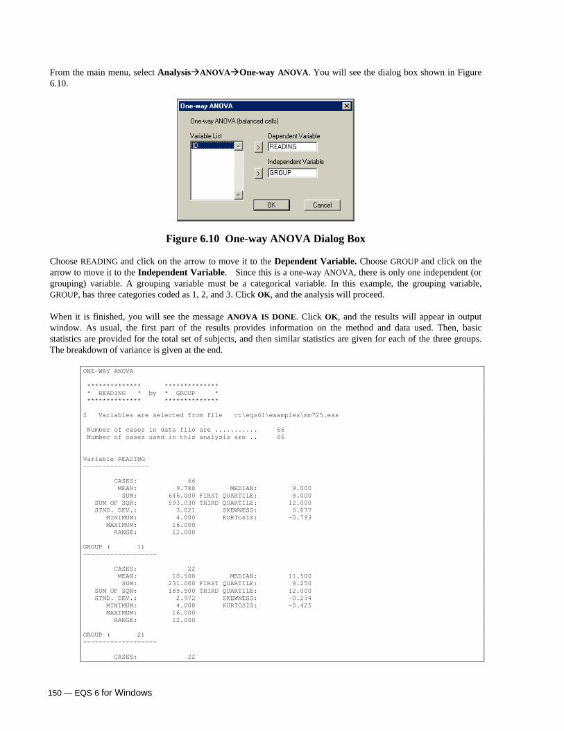
150 — EQS 6 for Windows
From the main menu, select Analysis ANOVA One-way ANOVA. You will see the dialog box shown in Figure 6.10.
Figure 6.10 One-way ANOVA Dialog Box Choose READING and click on the arrow to move it to the Dependent Variable. Choose GROUP and click on the arrow to move it to the Independent Variable. Since this is a one-way ANOVA, there is only one independent (or grouping) variable. A grouping variable must be a categorical variable. In this example, the grouping variable, GROUP, has three categories coded as 1, 2, and 3. Click OK, and the analysis will proceed. When it is finished, you will see the message ANOVA IS DONE. Click OK, and the results will appear in output window. As usual, the first part of the results provides information on the method and data used. Then, basic statistics are provided for the total set of subjects, and then similar statistics are given for each of the three groups. The breakdown of variance is given at the end.
ONE-WAY ANOVA ************** ************** * READING * by * GROUP * ************** ************** 2 Variables are selected from file c:\eqs61\examples\mm725.ess Number of cases in data file are ........... 66 Number of cases used in this analysis are .. 66 Variable READING ----------------- CASES: 66 MEAN: 9.788 MEDIAN: 9.000 SUM: 646.000 FIRST QUARTILE: 8.000 SUM OF SQR: 593.030 THIRD QUARTILE: 12.000 STND. DEV.: 3.021 SKEWNESS: 0.077 MINIMUM: 4.000 KURTOSIS: -0.793 MAXIMUM: 16.000 RANGE: 12.000 GROUP ( 1) ------------------- CASES: 22 MEAN: 10.500 MEDIAN: 11.500 SUM: 231.000 FIRST QUARTILE: 8.250 SUM OF SQR: 185.500 THIRD QUARTILE: 12.000 STND. DEV.: 2.972 SKEWNESS: -0.234 MINIMUM: 4.000 KURTOSIS: -0.425 MAXIMUM: 16.000 RANGE: 12.000 GROUP ( 2) ------------------- CASES: 22

EQS 6 for Windows — 151
MEAN: 9.727 MEDIAN: 9.000 SUM: 214.000 FIRST QUARTILE: 8.000 SUM OF SQR: 152.364 THIRD QUARTILE: 11.500 STND. DEV.: 2.694 SKEWNESS: 0.866 MINIMUM: 6.000 KURTOSIS: -0.149 MAXIMUM: 16.000 RANGE: 10.000 GROUP ( 3) ------------------- CASES: 22 MEAN: 9.136 MEDIAN: 8.500 SUM: 201.000 FIRST QUARTILE: 6.250 SUM OF SQR: 234.591 THIRD QUARTILE: 12.000 STND. DEV.: 3.342 SKEWNESS: 0.004 MINIMUM: 4.000 KURTOSIS: -1.401 MAXIMUM: 14.000 RANGE: 10.000 ANALYSIS OF VARIANCE ==================== Source SUM OF SQUARES DF MEAN SQUARES F p ___________________________________________________________________ GROUP 20.576 2 10.288 1.132 0.329 ERROR 572.455 63 9.087 TOTAL 593.030 65
The analysis of variance table reports the usual breakdown of the sum of squares into group (between-subject) and error (within-subjects) components, along with the associated degrees of freedom. The corresponding mean squares provide the basis for the F test. In this case F(2,63) = 1.132, with a probability value of .329, indicating that the null hypothesis of equal means cannot be rejected. Since this is a pretest, it shows that the groups are equal before the intervention takes place.
Two-Way Analysis of Variance In two-way analysis of variance, there are two categorical variables that represent group membership, and one dependent variable. The analysis aims to determine the effect of the categorical variables and their interaction on the dependent variable. In addition to partitioning the variance, statistical tests evaluate the null hypotheses that the main and interaction effects on the dependent variable are zero.
Note: This version of ANOVA handles only balanced cells. That is, the sample sizes in all cells must be equal. You cannot have a missing cell.
The file pancake.ess shows 24 case scores on three variables, QUALITY, SUPPLMNT, and WHEY, taken from Ryan, Joiner, & Ryan11. The data represent the effects of two factors, a food supplement and whey, on the rated quality of pancakes that were baked using various levels of these factors. There were four levels of whey and two levels of the supplement, so there are eight treatment combinations or cells. With three ratings in each cell, there are 8 × 3 = 24 overall quality ratings. The task is to determine the effects of the independent variables, and their interaction, on the rated quality of pancakes. As before, click on Analysis on the main menu, and then choose ANOVA Two-way ANOVA, the dialog box in Figure 6.11 will appear.
11 Ryan, B. F., Joiner, B. L., & Ryan Jr., T. A. (1992). MINITAB Handbook, 2nd Ed. Rev. Boston: PWS-Kent, p. 206.

152 — EQS 6 for Windows
Figure 6.11 Two-way ANOVA Dialog Box Choose QUALITY as the Dependent Variable, and SUPPLMNT and WHEY as the Independent Variables. Then click OK. The results of the ANOVA are, as usual, shown in output window. The format is very similar to that of the one-way analysis shown above. The summary statistics for the entire set of subjects are given first, and then statistics are given for each combination of independent variables. As just noted, SUPPLMNT has two levels and WHEY has four levels, so there are eight possible combinations of groups, and the output provides statistics for each such combination. To save space, only the first group’s summary is presented here followed by the ANOVA table.
TWO-WAY ANOVA ************** ************** ************** * QUALITY * by * SUPPLMNT * and * WHEY * ************** ************** ************** 3 Variables are selected from file c:\eqs61\examples\pancake.ess Number of cases in data file are ........... 24 Number of cases used in this analysis are .. 24 Variable QUALITY ----------------- CASES: 24 MEAN: 4.487 MEDIAN: 4.600 SUM: 107.700 FIRST QUARTILE: 4.175 SUM OF SQR: 11.406 THIRD QUARTILE: 4.850 STND. DEV.: 0.704 SKEWNESS: -0.546 MINIMUM: 3.100 KURTOSIS: -0.598 MAXIMUM: 5.600 RANGE: 2.500 SUPPLMNT ( 1) and WHEY ( 1) ------------------------------------------ CASES: 3 MEAN: 4.400 MEDIAN: 4.400 SUM: 13.200 FIRST QUARTILE: 4.350 SUM OF SQR: 0.020 THIRD QUARTILE: 4.450 STND. DEV.: 0.100 SKEWNESS: -0.000 MINIMUM: 4.300 KURTOSIS: -1.500 MAXIMUM: 4.500 RANGE: 0.200 SUPPLMNT ( 2) and WHEY ( 1) ------------------------------------------- CASES: 3 MEAN: 3.200 MEDIAN: 3.200 SUM: 9.600 FIRST QUARTILE: 3.150 SUM OF SQR: 0.020 THIRD QUARTILE: 3.250 STND. DEV.: 0.100 SKEWNESS: -0.000 MINIMUM: 3.100 KURTOSIS: -1.500 MAXIMUM: 3.300 RANGE: 0.200 SUPPLMNT ( 1) and WHEY ( 2) -------------------------------------------

EQS 6 for Windows — 153
CASES: 3 MEAN: 4.633 MEDIAN: 4.600 SUM: 13.900 FIRST QUARTILE: 4.550 SUM OF SQR: 0.047 THIRD QUARTILE: 4.700 STND. DEV.: 0.153 SKEWNESS: 0.382 MINIMUM: 4.500 KURTOSIS: -1.500 MAXIMUM: 4.800 RANGE: 0.300 SUPPLMNT ( 2) and WHEY ( 2) ------------------------------------------- CASES: 3 MEAN: 3.700 MEDIAN: 3.700 SUM: 11.100 FIRST QUARTILE: 3.650 SUM OF SQR: 0.020 THIRD QUARTILE: 3.750 STND. DEV.: 0.100 SKEWNESS: -0.000 MINIMUM: 3.600 KURTOSIS: -1.500 MAXIMUM: 3.800 RANGE: 0.200 SUPPLMNT ( 1) and WHEY ( 3) ------------------------------------------- CASES: 3 MEAN: 4.700 MEDIAN: 4.800 SUM: 14.100 FIRST QUARTILE: 4.650 SUM OF SQR: 0.060 THIRD QUARTILE: 4.800 STND. DEV.: 0.173 SKEWNESS: -0.707 MINIMUM: 4.500 KURTOSIS: -1.500 MAXIMUM: 4.800 RANGE: 0.300 SUPPLMNT ( 2) and WHEY ( 3) ------------------------------------------- CASES: 3 MEAN: 5.033 MEDIAN: 5.000 SUM: 15.100 FIRST QUARTILE: 4.900 SUM OF SQR: 0.127 THIRD QUARTILE: 5.150 STND. DEV.: 0.252 SKEWNESS: 0.239 MINIMUM: 4.800 KURTOSIS: -1.500 MAXIMUM: 5.300 RANGE: 0.500 SUPPLMNT ( 1) and WHEY ( 4) ------------------------------------------- CASES: 3 MEAN: 4.800 MEDIAN: 4.700 SUM: 14.400 FIRST QUARTILE: 4.650 SUM OF SQR: 0.140 THIRD QUARTILE: 4.900 STND. DEV.: 0.265 SKEWNESS: 0.595 MINIMUM: 4.600 KURTOSIS: -1.500 MAXIMUM: 5.100 RANGE: 0.500 SUPPLMNT ( 2) and WHEY ( 4) ------------------------------------------- CASES: 3 MEAN: 5.433 MEDIAN: 5.400 SUM: 16.300 FIRST QUARTILE: 5.350 SUM OF SQR: 0.047 THIRD QUARTILE: 5.500 STND. DEV.: 0.153 SKEWNESS: 0.382 MINIMUM: 5.300 KURTOSIS: -1.500 MAXIMUM: 5.600 RANGE: 0.300 ANALYSIS OF VARIANCE ==================== Source SUM OF SQUARES DF MEAN SQUARES F p ___________________________________________________________________ SUPPLMNT 0.510 1 0.510 17.014 0.001 WHEY 6.691 3 2.230 74.347 0.000 INTERACTION 3.725 3 1.242 41.384 0.000 ERROR 0.480 16 0.030 TOTAL 11.406 23 ___________________________________________________________________

154 — EQS 6 for Windows
General Linear Model This procedure, new in EQS 6, is capable of handling a wide variety of ANOVA models. It can handle both balanced and unbalanced designs. This method is capable of performing any factorial ANOVA including one-way and two-way ANOVAs. It is also capable of performing ANCOVA. Using the same data, pancake.ess, from the two-way ANOVA section, we will perform the same analysis using the general linear model procedure. First, open the pancake.ess dataset located in the example folder. Next click on Analysis ANOVA General Linear Model; you will see the dialog box in Figure 6.12.
Figure 6.12 General Linear Model Dialog Box
Choose QUALITY as the Dependent variable and SUPPLMNT and WHEY as the Independent variable(s). Then click OK. The results will be displayed in output window.
GENERAL LINEAR MODEL 3 Variables are selected from file c:\eqs61\examples\pancake.ess VARIABLE QUALITY Number of cases in data file are ........... 24 Number of cases used in this analysis are .. 24 Number of complete cases .................. 24 Number of observations .................... 24 Final status .............................. Convergence Maximized log likelihood .................. 12.8898 Akaike information criterion .............. 11.8898 Approximate convergence rate .............. 1.95e-013 Maximum number of iterations .............. 100 Maximum number of step halvings ........... 20 Convergence criterion for cov. parameters . 1e-005 Convergence criterion for log likelihood .. 1e-005 Tolerance for pivoting .................... 1e-006 Algorithm used ............................ Newton Raphson Covariance structure ...................... Unstructured Step Log Improvement Max. Rel. Change Iteration Halvings Likelihood in Log Lik. in Cov. Params. _______________________________________________________________ 0 0 -14.122 1 0 12.890 2.701e+001 2.974e-016 2 0 12.890 5.272e-012 9.474e-019 _______________________________________________________________ ANALYSIS OF VARIANCE ====================

EQS 6 for Windows — 155
Sum of Mean Source Squares DF Square F p ________________________________________________________________________ Intercept 483.304 1 483.304 16110.125 0.000 Main effects SUPPLMNT (S) 0.510 1 0.510 17.014 0.001 WHEY (W) 6.691 3 2.230 74.347 0.000 Interactions S.W 3.725 3 1.242 41.384 0.000 Error 0.480 16 0.030 ________________________________________________________________________ Wald Tests of Significance Source DF Chi-square p ___________________________________________ SUPPLMNT (S) 1 25.521 0.000 WHEY (W) 3 334.563 0.000 S.W 3 186.229 0.000 ___________________________________________ Estimates of Regression Parameters Asymptotic 95.0% Parameter Estimate Std. Err. Confidence Interval z p ________________________________________________________________________ Intercept 4.488 0.029 4.431 4.544 155.452 0.000 S1 0.146 0.029 0.089 0.202 5.052 0.000 W1 -0.687 0.050 -0.785 -0.590 -13.750 0.000 W2 -0.321 0.050 -0.419 -0.223 -6.417 0.000 W3 0.379 0.050 0.281 0.477 7.583 0.000 S1.W1 0.454 0.050 0.356 0.552 9.083 0.000 S1.W2 0.321 0.050 0.223 0.419 6.417 0.000 S1.W3 -0.313 0.050 -0.410 -0.215 -6.250 0.000 ________________________________________________________________________ Estimates of Residual Covariance Asymptotic 95.0% Parameter Estimate Std. Err. Confidence Interval z p _______________________________________________________________________ 1 0.020 0.006 0.009 0.031 3.464 0.001 _______________________________________________________________________
General linear model estimates are produced using a Newton-Raphson algorithm. The output shows that the iterations converged to a unique solution. Below the iteration history is the ANOVA table, including Wald statistics. Regression estimates are reported next. The estimates are produced using a default deviation contrast. A deviation contrast compares one group mean to the grand mean. For instance, in the example above, W1 (first contrast of whey) with the parameter estimate –0.687 is the difference between first level of whey and grand mean. One interpretation of the deviation contrast in this example could be comparison of first level of whey to all other levels combined. So that the hypothesis question would be, “is there a mean difference of quality between the first level of whey and all other levels combined?” In the example above, S1 to W3 represents marginal comparisons using the deviation contrasts. S1.W1 to S1.W3 represents interaction contrasts, created by multiplying the deviation contrasts of S (supplement) and W (whey).
Correlations and Covariances It is hard to imagine an analysis of non-experimental data that doesn’t require evaluating the correlations among variables, or, their unstandardized equivalents, the covariances. In EQS 6 for Windows, these computations are accomplished by selecting Analysis, then Correlations.

156 — EQS 6 for Windows
To illustrate the procedure, we shall use some data from page 3 of Mardia, Kent, & Bibby12. They provided exam grades for 88 students in five technical topics. The topics were mechanics, vectors, algebra, analysis, and statistics. One might expect that students who do relatively well in one of those quantitative areas would also do relatively well in the others. That is, we expect the variables to be substantially correlated. Open the mardia3.ess file now. You should see the 88 by 5 matrix in the Data Editor. Click on Analysis and then Correlations. You will see the dialog box shown in Figure 6.13.
Figure 6.13 Covariance/Correlation Matrix Dialog Box
Use the double right-arrow to move all the variables from the Variable List box to the Selection List box. Choose Correlation Matrix. To see the options available with this procedure, click on the Options button. Figure 6.14 will appear.
Figure 6.14 Covariance/Correlation Matrix Options Dialog Box
Missing Data in Covariance/Correlation By default, the computations use complete cases only, i.e., listwise deletion. The second option is pairwise deletion; correlations or covariances are computed for all subjects that have data for a given pair of variables.
12 Mardia, K. V., Kent, J. T., & Bibby, J. M. (1979). Multivariate Analysis. New York: Academic.

EQS 6 for Windows — 157
Cronbach’s Alpha To estimate the reliability of a sum computed across variables being correlated, click on the Cronbach’s Alpha option. Please click on this option now. The result will compute Cronbach’s alpha, a measure of internal consistency. In general, alphas based on correlation and covariance matrices will differ. The alpha based on the covariance matrix (i.e., unstandardized alpha) is a lower bound to the internal consistency of the raw-score sum. A sum based on standardized scores would require the use of the correlation matrix (i.e., standardized alpha).
Putting the Matrix in the Data Editor A valuable option is: Put matrix in a new data editor. Please click on this option now. With this option, not only do you receive the standard output in the output.log, but the matrix is also placed into the Data Editor under the name matrix.ess. The correlation or covariance matrix could be retrieved from this window when you do a factor analysis, or when you do structural modeling. Or, you can simply save your matrix. If you save it, use Save As and give in a new name; otherwise it will be overwritten the next time you use Put matrix in a new data editor. Click OK. When the computations are completed you will be told MATRIX DONE. Click OK to see the matrix displayed in Figure 6.15. It gives the symmetric matrix summarizing the correlations among all variables.
Figure 6.15 Correlation Matrix in Data Editor The output.log provides the same information as the matrix.ess file, but in a slightly different format. Only the lower triangle of correlations is printed.
CORRELATION MATRIX 5 Variables are selected from file c:\eqs61\examples\mardia3.ess Number of cases in data file are ........... 88 Number of cases used in this analysis are .. 88 C-Mechan C-Vector C-Algebr C-Analys O-Statis C-Mechan 1.0000 C-Vector 0.5534 1.0000 C-Algebr 0.5468 0.6096 1.0000 C-Analys 0.4094 0.4851 0.7108 1.0000 O-Statis 0.3891 0.4364 0.6647 0.6072 1.0000
As you can see, the output tells us the number of variables used, the data file used, the number of cases in the file, and the number of cases used. In this example, there are no missing data, so the numbers of cases match.

158 — EQS 6 for Windows
It is apparent that the students’ scores on these various tests are all positively correlated. The highest correlation is between the algebra and analysis tests. Don’t forget that these correlations could be affected substantially by a few cases that are outliers. To see if there are any outliers, and to determine the effect on the correlations, you can use, for example, the scatter plot icon. (Yes, there are some questionable cases here.) The procedures and output related to the computation of a covariance matrix are essentially the same. The output file will be titled appropriately, and you will see variances in the diagonal of the matrix, with covariances in the off-diagonal positions.
Regression Linear regression is used to predict a dependent variable from one or more independent variables. The procedure estimates the weight for each of the independent variables that would yield a predicted score for each case that is as close as possible to the actual dependent variable score, using a least-squares criterion. We shall illustrate this method using the file chatter.ess. The reference, and an explanation of the variables, can be found in the Descriptive Statistics section at the start of this chapter. Please Open the file chatter.ess now. It is a small dataset, but the authors used it effectively to show potential problems with the blind use of linear regression. We will not discuss those problems here; see the reference if you are interested. Click on Analysis Regressions. EQS is capable of performing three different types of regression: standard, stepwise, and hierarchical. If you click on Standard Multiple Regression, you will see the dialog box shown in Figure 6.16. Choose VAR4 as the Dependent Variable and VAR1-VAR3 as the Independent Variable(s).
Figure 6.16 Standard Multiple Regression Dialog Box In addition, you see the check box Add regression estimates and residuals to data sheet. Please click on it. This choice will add two columns to the Data Editor. The columns will be the predicted scores (for VAR4 in this example) and the residuals (VAR4 minus predicted VAR4). This option makes these new scores available for plotting and, indeed, for any other purpose for which data scores might be used. When you click OK, the computations begin. Almost immediately, you will see the message, MULTIPLE REGRESSION DONE . When you click OK, you will see the following results in output window.
STANDARD MULTIPLE REGRESSION 4 Variables are selected from file c:\eqs61\examples\chatter.ess

EQS 6 for Windows — 159
Number of cases in data file are ........... 24 Number of cases used in this analysis are .. 24 ANALYSIS OF VARIANCE ==================== Source SUM OF SQUARES DF MEAN SQUARES F p ___________________________________________________________________ REGRESSION 4433.166 3 1477.722 14.525 0.000 RESIDUAL 2034.667 20 101.733 TOTAL 6467.833 23 ___________________________________________________________________ Dependent Variable = VAR4 Number of obs. = 24 Multiple R = 0.8279 R-square = 0.6854 Adjusted R-square = 0.6382 F( 3, 20) = 14.5254 Prob > F = 0.0000 Std. Error of Est. = 10.0863 Durbin-Watson Stat.= 1.5764 =======REGRESSION COEFFICIENTS======= HETERO- ORDINARY SCEDASTIC VARIABLE B STD. ERROR STD. ERROR BETA t p _______________________________________________________________________ Intercept 156.622 22.605 21.859 7.165 0.000 VAR1 -1.153 0.279 0.296 -0.657 -3.901 0.001 VAR2 -0.265 0.544 0.613 -0.083 -0.433 0.670 VAR3 -15.594 7.243 7.645 -0.294 -2.040 0.055 _______________________________________________________________________
First, you get the analysis of variance, which tests whether we can reject the null hypothesis that the coefficients are zero. In this example, the p-value from the F-test is tiny, so the null hypothesis can be rejected. Next, there is a section that summarizes various statistics whose precise definition is given in standard texts and the BMDP Statistical Software Manual. The most important of these are the R-square and the Adjusted R-square. Next you will see the estimated regression coefficients, in both the unstandardized form, (B), and then in the standardized form, (BETA). The sign of each of the regression weights is negative (in the original report, one was given as positive). Two-tailed significance tests on the regression coefficients are given on the right. V2 has no significant effect on V4 in the context of the other predictors. A new addition to EQS 6 in multiple regression is the reporting of the heteroscedastic standard error. If you violate the assumption of homoscedasticity in multiple regression, you can adjust the standard error and still analyze the data. The t values are computed using the heteroscedastic standard error. This adjustment was first reported by Efron (1982)13, however, for more current discussion of the issue refer to Long and Ervin (2000)14. The heteroscedastic standard error computed in EQS is the HC3 formula of Long and Ervin (p. 218).
Estimates and Residuals in Data Editor As stated above, the option to Add regression estimates and residuals to data sheet modifies the input data file in the Data Editor by adding two columns of numbers. You will see this if you go back to the Window option, and select the window chatter.ess.
13 Efron, B. (1982). The Jackknife, Bootstrap and other Resampling Plans. Philadelphia: SIAM. 14 Long, J. S., & Ervin, L. H. (2000). Using heteroscedasticity consistent standard errors in the linear regression model. The American Statistician, 54 (3), 217-224.

160 — EQS 6 for Windows
An illustration is provided in Figure 6.17, which shows the new data variables YEST1A and RESID1A, the default names used in the program for the estimated and residual variables from the regression. If you were to do other regression analyses (or any other analyses) with the chatter.ess file, you could use these variables just like any other variables. If you were to do another regression, again requesting estimates and residuals to be added to the Data Editor, those new variables would be added to the previously existing variables. Of course, you can eliminate any column in the Data Editor with the usual Edit and Delete commands, after highlighting the column by clicking on the appropriate variable name.
Figure 6.17 Estimates and Residuals in the Data Editor As you see in Figure 6.17, the estimates and residuals are added to the observed variable scores. For case 1, the estimate is 55.5461, and the residual is 11.4539. Their sum equals 67, which is the value of VAR4. Of course, the smaller the residuals, the better the regression equation has predicted the dependent variable.
Plotting Residuals and Predictors You may remember that predicted and residual scores in regression should be independent. You can check this assumption yourself by choosing the scatter plot icon, and plotting these two variables against each other (see Figure 6.18). You will find that the correlation between the variables is indeed zero, and the regression line is completely flat. If you do not remember this fact from regression, the plot will quickly remind you.
Figure 6.18 Scatter Plot of Predicted V4 and Residual in chatter.ess
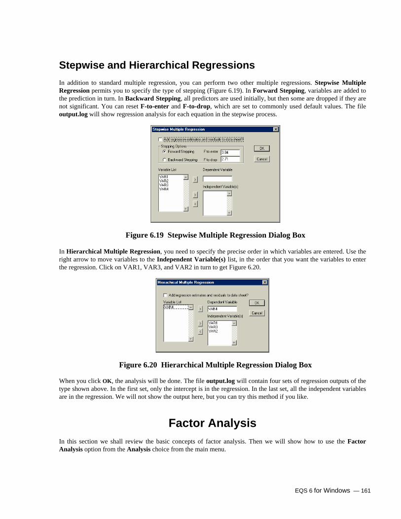
EQS 6 for Windows — 161
Stepwise and Hierarchical Regressions In addition to standard multiple regression, you can perform two other multiple regressions. Stepwise Multiple Regression permits you to specify the type of stepping (Figure 6.19). In Forward Stepping, variables are added to the prediction in turn. In Backward Stepping, all predictors are used initially, but then some are dropped if they are not significant. You can reset F-to-enter and F-to-drop, which are set to commonly used default values. The file output.log will show regression analysis for each equation in the stepwise process.
Figure 6.19 Stepwise Multiple Regression Dialog Box In Hierarchical Multiple Regression, you need to specify the precise order in which variables are entered. Use the right arrow to move variables to the Independent Variable(s) list, in the order that you want the variables to enter the regression. Click on VAR1, VAR3, and VAR2 in turn to get Figure 6.20.
Figure 6.20 Hierarchical Multiple Regression Dialog Box When you click OK, the analysis will be done. The file output.log will contain four sets of regression outputs of the type shown above. In the first set, only the intercept is in the regression. In the last set, all the independent variables are in the regression. We will not show the output here, but you can try this method if you like.
Factor Analysis In this section we shall review the basic concepts of factor analysis. Then we will show how to use the Factor Analysis option from the Analysis choice from the main menu.

162 — EQS 6 for Windows
A model that relates measured variables to latent factors is called a measurement model. Most measurement models are just factor analysis models, but it is standard to distinguish between confirmatory and exploratory factor analysis.
Confirmatory Models Created with Build_EQS Option Measurement models used in structural modeling are confirmatory factor analysis models. In confirmatory factor analysis, the researcher presumably knows—or at least, has a strong hypothesis about—the number of factors necessary to explain the intercorrelations among variables. In addition, one knows which measured variables are supposedly good indicators of each of the factors, and which variables are unrelated to a factor. In confirmatory models, variables are often presumed to be factorially simple. That is, a given variable is usually expected to be influenced by very few factors, typically only one. Path diagram representations of factor analysis usually imply confirmatory factor models, since they are very specific about these details. Of course, a researcher’s hypotheses may be incorrect. The structural modeling evaluation will provide evidence of the adequacy of the hypotheses. To perform a confirmatory factor analysis, use the structural modeling part of EQS 6 for Windows, Build_EQS on the main menu.
Exploratory Models Created with Factor Analysis Option On the other hand, factor analysis is most frequently done in an exploratory mode. In an exploratory factor analysis, one suspects that variables correlate because there are one or several underlying latent factors that generate the observed data. We may have a vague, imprecise idea about this. We may suspect that there are one or several factors, but we may not know precisely how many factors are needed to explain the intercorrelations among variables. Perhaps there is one factor; perhaps there are five factors. In addition, even if we are pretty sure about the existence of a particular factor, we may not know which variables are the best indicators of the factor. The Factor Analysis option of the Analysis menu does an exploratory factor analysis.
The Basics of Factor Analysis Before we go into operational details, we review some of the basic ideas of factor analysis to be sure that you know what is reasonable to expect from a factor analysis, and what is not. This is not the place to provide a discourse on factor analysis, but you must know certain basic facts about the methodology in order to use latent variables effectively. Those of you who are knowledgeable can, of course, skip these sections.
What Factors Imply about Variables It is often said that factors explain the correlations among variables. Let us expand on this idea, using path diagram notation without the underlying mathematics. In general, you have a path diagram containing a latent factor, called an F variable in EQS. Arrows emanate from that latent factor and aim at several V variables, or measured variables in EQS. When you have such a diagram, you are making the strong claim that these particular V variables are highly intercorrelated (the sign, + or -, of a correlation is irrelevant here). For example, in the diagram V1 F V2, the factor F generates the two measured variables V1 and V2. The reason for their intercorrelation is that the same F generates these Vs. Stated differently, if the F variable were controlled, or eliminated statistically, the V variables would no longer correlate. This is the meaning of the first factor ever

EQS 6 for Windows — 163
hypothesized, the IQ or general intelligence factor. According to the general intelligence hypothesis, the IQ factor generates the correlation among various indicators of intellectual performance. In the typical case, there will be many variables and more than one factor. In addition to claiming that V1 and V2 are correlated because they share the same factor, you also are making the claim that these V variables have relatively low correlations with other V variables that are not directly influenced by this same factor. When studying intelligence, if V3 and V4 are nonintellectual variables, such as attitudes toward school and studying, then V3 and V4 would be expected to be less highly correlated with the intellectual variables V1 and V2 than the intellectual variables would correlate among themselves. When you have several factors, such as F1, F2, and F3, and have different indicators for each factor (e.g., V1, V2, V3 are indicators of F1; V4, V5, V6 are indicators of F2; and V7, V8, and V9 are indicators of F3), a substantial number of such predictions are implied by the factor analysis model.
Choosing Between Exploratory and Confirmatory Models When you do an exploratory factor analysis, you may be uncertain about the types of claims you can make about the correlations among your variables. The factor analysis will give you results: the number of factors, the factor loadings, and possibly the factor correlations. These will permit you to make statements such as those above, illustrating how the variables are, in fact, generated from your data. If you know enough about your data to anticipate these results, you should skip the exploratory step and do a confirmatory factor analysis. That is, if you have a good idea about the expected number of factors to be found, and the variables that you expect to be highly influenced by a particular factor, you need not bother with an exploratory analysis.
The Naming Fallacy There are two aspects to what we call a naming fallacy. We must be careful to avoid these fallacies. Both of them can interfere with our understanding of the data.
1. After giving a particular name to a set of variables, we conclude that these variables must share a factor.
2. After finding a factor analysis result, we know which variables are highly correlated with the factor, so we think we know what the factor is.
First, before you do an analysis, you may expect a factor to appear because of some shared feature of your data. This may be a naive expectation. You need to be sure that you have worked through the various implications of what factors imply about variables, as we summarized above. For example, suppose that you have given a similar name to a particular set of variables (e.g., V1 through V5 are all “demographics” and V6-V9 represent “attitude”). Does this mean that you should expect to see a “demographic” factor and an “attitude” factor? Perhaps, if your subjects happen to respond in such a way as to create high correlations among the variables within each set, and lower correlations between the sets. On the other hand, the names may simply mislead you. For example, the demographics of subjects’ height and number of children in the family are likely to be uncorrelated. No matter that they are both “demographic” variables, sharing a name, these variables most likely will not form a factor. It does not seem probable that taller children come from families with more (or fewer) children.
Factor Indeterminacy

164 — EQS 6 for Windows
After an analysis in which you see that several Vs are good indicators of a factor, you may become convinced that you understand the factor. It is, after all, whatever the variables share in common. But there is an extensive technical literature on the topic called factor indeterminacy. The literature implies that you can become certain about what a factor is only when the number of variables that have high factor loadings on that factor increases without limit. In practice, you will have only a few good indicators of a given factor. The nature of the first, and most famous of all factors, general intelligence, is still being debated today; so don’t claim too much knowledge about your own factors.
Exploratory vs. Confirmatory Factor Analysis We can now expand on the earlier discussion of exploratory and confirmatory factor analysis. A structural modeling analysis that tests a completely a priori theory does not need to rely on an exploratory factor analysis. The model can simply be specified and tested using Build_EQS. In fact, an exploratory factor analysis may not be able to capture the structure implied by some measurement designs. In contrast, a confirmatory factor analysis could represent the relations of variables to factors. Whether exploratory or confirmatory factor analysis is appropriate for your situation will depend on your objectives and your state of knowledge about your data.
Highly Structured Measurement Models In general, models that are more appropriate to confirmatory than exploratory methods are highly specialized structural measurement models. Such models contain many factors relative to number of variables, or have a highly complex loading pattern on the basis of the design of the variables. The multitrait-multimethod model is an example of a highly specialized structural measurement model. In such a model, V variables are generated under a systematic design in which certain methods of measurement (e.g., self-report, behavioral observation, physiological scores) are fully crossed with the trait variables intended to be measured (e.g., anxiety, aggression, depression). That is, each trait is measured by each of several methods. When this design applies, factors can be hypothesized to separate the various sources of variance, especially, into trait and method factors. Interest is usually on the trait factors, while the method factors are usually of little substantive interest. However, the method factors are needed in the analysis, since they provide an important basis for correlations among variables.
Note: An exploratory factor analysis generally cannot find or verify such a specialized loading pattern. You must do a confirmatory factor analysis.
A confirmatory factor analysis can help you to clarify the measurement structure of your variables, whether in the context of a measurement model or a general model that also contains some factors. But be careful about claiming too much from a measurement model. As noted with regard to the naming fallacy, the nature of a factor may remain obscure until further research is done. In a multitrait-multimethod model, for example, you may find a “physiological” factor. But what does it mean? The body’s physiology is quite complex.
The Factor Model within a General Model When working with a general structural model, you may be interested in determining whether the measurement part of your model is correct. This could be done by exploratory or confirmatory methods, depending on the structure you hypothesize. If you know little about your variables, or your measurement structure is very simple, an exploratory factor analysis should be fine. But if your measurement hypothesis is complicated, you may not get evidence about your hypotheses without doing a confirmatory analysis.

EQS 6 for Windows — 165
Even if you do not have a specialized, complex factor loading pattern in mind, you may be able to specify precisely the pattern of fixed and free-to-be-estimated factor loadings in your measurement model, as part of some larger structural model. Then you can transform any latent variable structural model into a confirmatory factor model by eliminating the regressions among factors, and changing all dependent F variables into independent F variables. Generally, you should let all of these factors covary. Such a measurement model without equations for Fs is a confirmatory factor analysis model. If you can specify such a model, don’t waste your time with exploratory factor analysis. The results of a modeling run should be good enough to provide evidence on the empirical validity of your measurement hypotheses.
On Modifying a Bad Measurement Model When running a confirmatory factor analysis, or any other specific a priori structural model, the model either will fit the data well from a statistical point of view, or it will not fit the data well. Of course, if the model does not fit, it could be due to one of three causes:
1. The measurement model is in some way flawed. 2. The hypothesized relations among factors are not consistent with the data. 3. Other paths and covariances are misspecified.
If you have no theoretical way to modify your a priori model, it may be necessary to rely on model modification procedures such as Lagrange Multiplier (LM) or Wald (W) tests. If you have minor problems in your model, these tests will help you to modify the model so that it is more consistent with your data. See the EQS 6 Structural Equations Program Manual for more information. Often, however, LM and W tests are not as good as an exploratory factor analysis in finding flaws in a measurement model. For example, you might have a model that specifies three factors, but there really are four or five factors in your data. Then an exploratory factor analysis will inform you about this situation much more effectively than any confirmatory factor analysis, or even the most creative use of the LM test. In conclusion, an exploratory factor analysis may be a useful precursor to further modeling work when:
1. You do not know much about the number of factors of a given set of variables. 2. You do not know which variables provide especially good indicators of your various factors.
Factor Analysis in EQS 6 for Windows
Background EQS 6 for Windows provides two extraction methods that are very fast and reliable, principal components analysis and Equal Prior Instant Communalities (EPIC). They typically yield a very good approximation to more complex methods available in packages such as SPSS for Windows. If you plan to do modeling with latent variables, you should not choose principal components. You should use the EPIC method instead.
Initial Unrotated Factor Solution

166 — EQS 6 for Windows
The initial unrotated factor solution is based on two different extraction methods. Principal components analysis is a very common method of extracting components, but is not considered to be true factor analysis. It is most appropriate when the number of variables is very large and only a few components are needed. The EPIC solution is a true factor analysis solution in which the unique variances are initially taken as equal. Based on adjusted principal components, the computations can be done explicitly and quickly. Kaiser proposed using this method for its ability to be untroubled by linear dependencies among variables, by improper solutions with negative variance estimates, or failure to converge. He reported that EPIC solutions are very close to that which experts consider subjectively to be optimum. See Kaiser15. The method was discussed previously by others, especially Anderson16. The mathematical rationale for the computations done in EQS 6 for Windows can be found in Anderson (p. 21). A thorough comparison of this method with others is given in Hayashi and Bentler (2000.)17 EPIC gains freedom from computational difficulties at a price: the unique variances of the correlation matrix are presumed to be equal under the model. There are three reasons why this assumption is not as restrictive as it seems:
1. The unique variances for the covariance matrix, not used in the computations, are not presumed to be equal under the model. Rather, the ratio of common factor variance to unique variance is hypothesized as equal for all variables under the model.
2. The estimated communalities of the correlation matrix, obtained from the solution, can vary substantially in practice.
3. For a small number of factors, the distortion induced by the restricted hypothesis becomes trivial, as the number of variables gets large.
Rotated Factor Solution There are three rotation methods available in EQS 6 for Windows. Two are orthogonal, varimax and orthosim, and one is oblique, direct oblimin. The orthosim rotation produces results that are very similar to those produced by varimax, the standard in the field18. Despite its age, the direct oblimin solution remains one of the best available19. Although varimax is the EQS default to permit easy comparison to the default options in other programs, it is not the wisest choice in the modeling context, since it forces factors to be uncorrelated. Factors used in models almost always allow non-zero correlations. You can change the default to oblimin by changing your Preferences (see Chapter 10.)
Factor Analysis Dialog Box You can run factor analysis from the main menu. As always, you must activate a data file before specifying the analysis. Please bring up the mardia3.ess file at this time. As you saw when we introduced this file in the section on correlations, above, it has the scores of 88 cases on five variables. Select Analysis and click on the option Factor Analysis. You will see the dialog box shown in Figure 6.21.
15 Kaiser, H. F. (1990). Outline of EPIC, a new method for factoring a reduced correlation matrix.... Paper presented at Society of Multivariate Experimental Psychology, Providence, RI, October, 1990. 16 Anderson, T. W. (1984). Estimating linear statistical relationships. Annals of Statistics, 12, 1-45. 17 Hayashi, K. & Bentler, P. M. (2000). On the relations among regular, equal unique variances, and image factor analysis models. Psychometrika, 65, 59-72. 18 Bentler, P. M. (1977). Factor simplicity index and transformations. Psychometrika, 42, 277-295. 19 Jennrich, R. I., & Sampson, P. F. (1966). Rotation to simple loadings. Psychometrika, 31, 313-323.
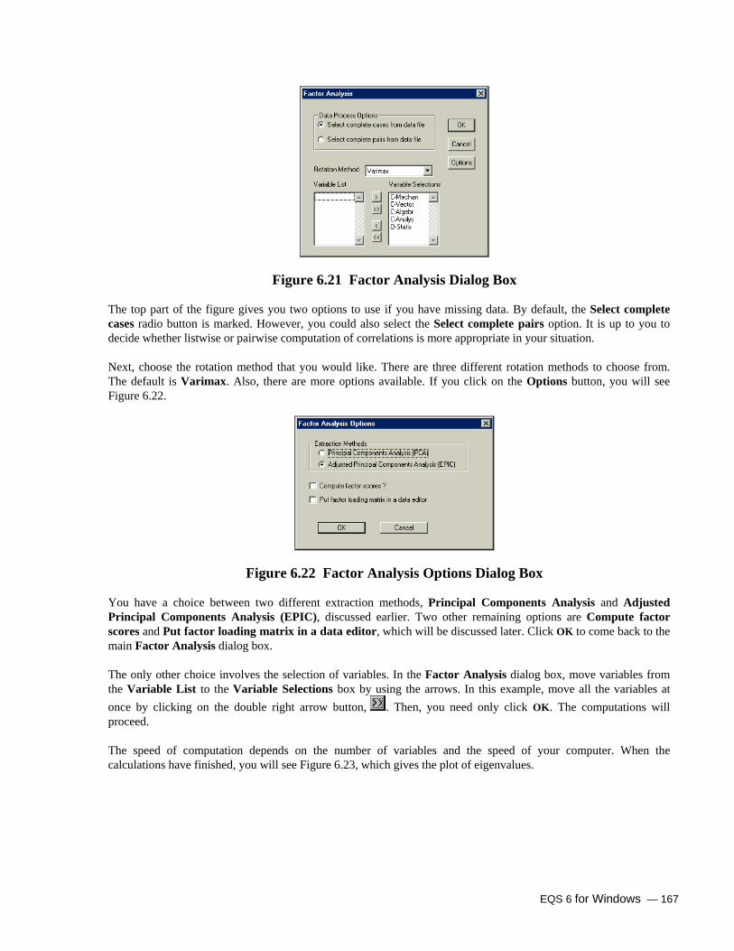
EQS 6 for Windows — 167
Figure 6.21 Factor Analysis Dialog Box The top part of the figure gives you two options to use if you have missing data. By default, the Select complete cases radio button is marked. However, you could also select the Select complete pairs option. It is up to you to decide whether listwise or pairwise computation of correlations is more appropriate in your situation. Next, choose the rotation method that you would like. There are three different rotation methods to choose from. The default is Varimax. Also, there are more options available. If you click on the Options button, you will see Figure 6.22.
Figure 6.22 Factor Analysis Options Dialog Box You have a choice between two different extraction methods, Principal Components Analysis and Adjusted Principal Components Analysis (EPIC), discussed earlier. Two other remaining options are Compute factor scores and Put factor loading matrix in a data editor, which will be discussed later. Click OK to come back to the main Factor Analysis dialog box. The only other choice involves the selection of variables. In the Factor Analysis dialog box, move variables from the Variable List to the Variable Selections box by using the arrows. In this example, move all the variables at once by clicking on the double right arrow button, . Then, you need only click OK. The computations will proceed. The speed of computation depends on the number of variables and the speed of your computer. When the calculations have finished, you will see Figure 6.23, which gives the plot of eigenvalues.

168 — EQS 6 for Windows
Figure 6.23 Factor Analysis — Plot of Eigenvalues
Selecting Number of Factors This plot shows the relative size of the eigenvalues of the correlation matrix. A red dotted line shows the Guttman-Kaiser criterion, eigenvalue > 1. By this criterion, there is only one factor. To get more information, click on Work Factor Specifications from the menu bar. When you do so, you will see the following dialog box.
Figure 6.24 Factor Analysis Selection Box Initially, the Number of Factors is marked at 1, and the Cut-off Eigenvalue is 3.181, which is the only eigenvalue greater than 1.0. If you enter 2 in the edit box Number of Factors, the Cut-off Eigenvalue box automatically shows 0.740; see Figure 6.24. The cut-off eigenvalue will automatically display the correct corresponding value.
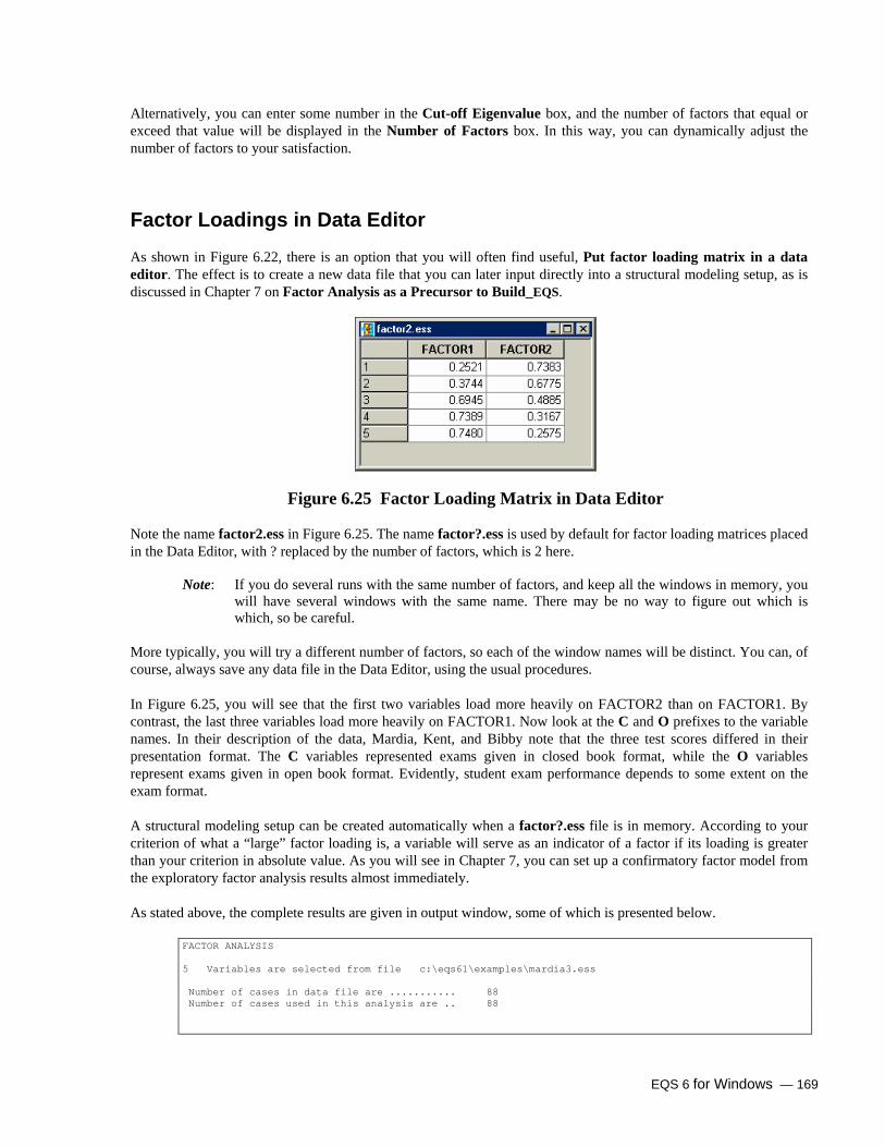
EQS 6 for Windows — 169
Alternatively, you can enter some number in the Cut-off Eigenvalue box, and the number of factors that equal or exceed that value will be displayed in the Number of Factors box. In this way, you can dynamically adjust the number of factors to your satisfaction.
Factor Loadings in Data Editor As shown in Figure 6.22, there is an option that you will often find useful, Put factor loading matrix in a data editor. The effect is to create a new data file that you can later input directly into a structural modeling setup, as is discussed in Chapter 7 on Factor Analysis as a Precursor to Build_EQS.
Figure 6.25 Factor Loading Matrix in Data Editor Note the name factor2.ess in Figure 6.25. The name factor?.ess is used by default for factor loading matrices placed in the Data Editor, with ? replaced by the number of factors, which is 2 here.
Note: If you do several runs with the same number of factors, and keep all the windows in memory, you will have several windows with the same name. There may be no way to figure out which is which, so be careful.
More typically, you will try a different number of factors, so each of the window names will be distinct. You can, of course, always save any data file in the Data Editor, using the usual procedures. In Figure 6.25, you will see that the first two variables load more heavily on FACTOR2 than on FACTOR1. By contrast, the last three variables load more heavily on FACTOR1. Now look at the C and O prefixes to the variable names. In their description of the data, Mardia, Kent, and Bibby note that the three test scores differed in their presentation format. The C variables represented exams given in closed book format, while the O variables represent exams given in open book format. Evidently, student exam performance depends to some extent on the exam format. A structural modeling setup can be created automatically when a factor?.ess file is in memory. According to your criterion of what a “large” factor loading is, a variable will serve as an indicator of a factor if its loading is greater than your criterion in absolute value. As you will see in Chapter 7, you can set up a confirmatory factor model from the exploratory factor analysis results almost immediately. As stated above, the complete results are given in output window, some of which is presented below.
FACTOR ANALYSIS 5 Variables are selected from file c:\eqs61\examples\mardia3.ess Number of cases in data file are ........... 88 Number of cases used in this analysis are .. 88

170 — EQS 6 for Windows
C-Mechan C-Vector C-Algebr C-Analys O-Statis C-Mechan 1.0000 C-Vector 0.5534 1.0000 C-Algebr 0.5468 0.6096 1.0000 C-Analys 0.4094 0.4851 0.7108 1.0000 O-Statis 0.3891 0.4364 0.6647 0.6072 1.0000 Eigenvalues 1 3.181 2 0.740 3 0.445 4 0.388 5 0.247 Number of factors selected are ....... 2 Constant for non-selected eigenvalues= 0.360 COMPONENT MATRIX (PRINCIPAL COMPONENTS) FACTOR 1 FACTOR 2 _______________________________ C-Mechan 0.713 -0.555 C-Vector 0.769 -0.380 C-Algebr 0.898 0.111 C-Analys 0.815 0.334 O-Statis 0.782 0.405 _______________________________ Communal. Prop. Cum.Prop. _________________________________________ C-Mechan 0.816 0.208 0.208 C-Vector 0.736 0.188 0.396 C-Algebr 0.818 0.209 0.605 C-Analys 0.776 0.198 0.802 O-Statis 0.775 0.198 1.000 _________________________________________ Variance Explained by Each Factor: FACTOR 1 FACTOR 2 _______________________________ 3.181 0.740 _______________________________ Total: 3.921 COMPONENT MATRIX (ADJUSTED COMPONENTS) [Used in calculations below] FACTOR 1 FACTOR 2 _______________________________ C-Mechan 0.671 -0.398 C-Vector 0.725 -0.272 C-Algebr 0.845 0.080 C-Analys 0.768 0.239 O-Statis 0.736 0.290 _______________________________ Communal. Prop. Cum.Prop. _________________________________________ C-Mechan 0.609 0.190 0.190 C-Vector 0.599 0.187 0.377 C-Algebr 0.721 0.225 0.603 C-Analys 0.646 0.202 0.804 O-Statis 0.626 0.196 1.000 _________________________________________ Variance Explained by Each Factor: FACTOR 1 FACTOR 2 _______________________________ 2.821 0.380 _______________________________

EQS 6 for Windows — 171
Total: 3.201 FACTOR LOADINGS (KAISER VARIMAX SOLUTION) Converge after 2 iterations FACTOR 1 FACTOR 2 _______________________________ C-Mechan 0.252 0.738 C-Vector 0.374 0.677 C-Algebr 0.694 0.488 C-Analys 0.739 0.317 O-Statis 0.748 0.258 _______________________________ Communal. Prop. Cum.Prop. _________________________________________ C-Mechan 0.609 0.190 0.190 C-Vector 0.599 0.187 0.377 C-Algebr 0.721 0.225 0.603 C-Analys 0.646 0.202 0.804 O-Statis 0.626 0.196 1.000 _________________________________________ Variance Explained by Each Factor: FACTOR 1 FACTOR 2 _______________________________ 1.792 1.409 _______________________________ Total: 3.201 FACTOR TRANSFORMATION MATRIX FACTOR 1 FACTOR 2 FACTOR 1 -0.760 FACTOR 2 -0.649 -0.760 FACTOR SCORE COEFFICIENTS FACTOR 1 FACTOR 2 _______________________________ C-Mechan -0.189 0.546 C-Vector -0.066 0.428 C-Algebr 0.272 0.091 C-Analys 0.393 -0.089 O-Statis 0.431 -0.148 _______________________________
In general, the output is self-explanatory. It contains information on the input data being used, the correlation matrix, its eigenvalues, the number of factors requested, and the constant that is the mean of the rejected eigenvalues (here, #3 - #5), used in computing the initial loading matrix. Finally, initial rotated solutions are presented. These are standard matrices interpreted in the usual way.
Factor Scores EQS 6 for Windows has an option to compute (really, “estimate”) factor scores. Factor scores are the unknown scores of the subjects on the latent factors. Unfortunately, true factor scores are always unknown, and the best that can be done is to estimate or predict them. EQS 6 uses a modified Bartlett (1937)20 estimator for this purpose.
20 Bartlett, M. S. (1937). The statistical conception of mental factors. British Journal of Psychology, 28, 97-104.
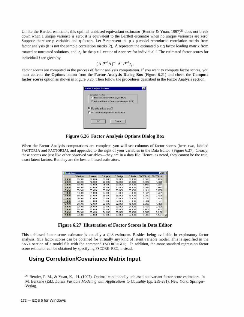
172 — EQS 6 for Windows
Unlike the Bartlett estimator, this optimal unbiased equivariant estimator (Bentler & Yuan, 1997)21 does not break down when a unique variance is zero; it is equivalent to the Bartlett estimator when no unique variances are zero. Suppose there are p variables and q factors. Let P represent the p x p model-reproduced correlation matrix from factor analysis (it is not the sample correlation matrix R), Λ represent the estimated p x q factor loading matrix from rotated or unrotated solutions, and iz be the p x 1 vector of z-scores for individual i. The estimated factor scores for individual i are given by
'P−1 −1(Λ Λ) 1' iP z−Λ . Factor scores are computed in the process of factor analysis computation. If you want to compute factor scores, you must activate the Options button from the Factor Analysis Dialog Box (Figure 6.21) and check the Compute factor scores option as shown in Figure 6.26. Then follow the procedures described in the Factor Analysis section.
Figure 6.26 Factor Analysis Options Dialog Box When the Factor Analysis computations are complete, you will see columns of factor scores (here, two, labeled FACTOR1A and FACTOR2A), and appended to the right of your variables in the Data Editor (Figure 6.27). Clearly, these scores are just like other observed variables—they are in a data file. Hence, as noted, they cannot be the true, exact latent factors. But they are the best unbiased estimators.
Figure 6.27 Illustration of Factor Scores in Data Editor This unbiased factor score estimator is actually a GLS estimator. Besides being available in exploratory factor analysis, GLS factor scores can be obtained for virtually any kind of latent variable model. This is specified in the SAVE section of a model file with the command FSCORE=GLS;. In addition, the more standard regression factor score estimator can be obtained by specifying FSCORE=REG; instead.
Using Correlation/Covariance Matrix Input
21 Bentler, P. M., & Yuan, K. –H. (1997). Optimal conditionally unbiased equivariant factor score estimators. In M. Berkane (Ed.), Latent Variable Modeling with Applications to Causality (pp. 259-281). New York: Springer-Verlag.

EQS 6 for Windows — 173
There is no need to use the raw data matrix for input into factor analysis. You also have the choice of using the derived correlation or covariance matrix. If you are going to be doing many factor analyses of a very large dataset, it is certainly better to use the correlation or covariance matrix. When you do that, you avoid computing the correlation matrix each time. With smaller datasets, or a very fast computer, using the raw data file does not really cause any slowdown worth worrying about. We can illustrate the procedure by starting from scratch with the mardia3.ess data. Choose Window to activate and close each window associated with the recent factor analysis. Choose Window and mardia3.ess to bring up the data file again. Select Analysis, then Correlations, and choose Correlation Matrix and Put matrix in new data editor options. Click on OK. Move all variables into the Selection List and click OK. You will get the 5-variable correlation matrix called matrix.ess (same as Figure 6.15). This is the default name for a correlation matrix that can be put into the factor analysis procedure. Of course, you could rename this file with any other *.ess designation. With matrix.ess as the active window, click on Analysis, and then Factor Analysis. The entire set of options and results in factor analysis, as described above, are available to you. We do not repeat them here. You can also compute the covariance matrix rather than the correlation matrix and save it as matrix.ess or with any other relevant file name. EQS 6 for Windows knows whether the data file being analyzed is a raw score data file, a correlation matrix, or a covariance matrix, and the program acts accordingly. Thus, covariance matrix input will yield the same results that we have already described.
Nonparametric Analyses There are three types of nonparametric statistical procedure in EQS 6 for Windows:
1. within-subjects comparisons 2. between-subjects comparisons 3. correlations.
We will demonstrate some of these options using a small dataset. (Caution: the procedure may be inappropriate for the data. It is for demonstration purposes only.) Open the same dataset used in correlation and covariance section, mardia3.ess. Click on Analysis Nonparametric Tests. The following dialog box will appear.
Figure 6.28 Nonparametric Statistics Dialog Box

174 — EQS 6 for Windows
To perform the tests, move the variables from Variable List to Test Variable(s). Next, place a check mark next to each test you would like to perform. For Kruskal-Wallis, you must define a Grouping Variable. For information about the nonparametric tests computed by EQS 6 for Windows, please consult any nonparametric statistics text (e.g., Conover (1998)22). Within-Subject Comparisons
1. Sign test 2. Wilcoxon signed-rank test 3. Kolmogorov-Smirnov two-sample test 4. Friedman’s two-way ANOVA by Ranks
Between-Subjects Comparisons
1. Kruskal-Wallis one-way ANOVA Correlations
1. Spearman rank correlation 2. Kendall rank correlation
The outputs are reported in the output window. Outputs for Sign, Wilcoxon, Kolmogrov-Smirnov, Spearman, and Kendall are reported similarly. They are all displayed in matrix format, where a column is compared (or computed) with a row variable. The test values are followed by matrix of significances (p-values). For example, in the Sign Test Results output below, Number of Nonzero Differences between C-Mechan and C-Vector is 81 of which 18 are positive. The comparison between C-Mechan and O-Statis produced 87 nonzero differences, of which 40 are positive. The first comparison, C-Mechan and C-Vector, is significant, p = 0.0000 while the second comparison, C-Mechan and O-Statis, is not significant, p = 0.5203.
Sign Test Results Number of Nonzero Differences C-Mechan C-Vector C-Algebr C-Analys O-Statis C-Mechan 0 C-Vector 81 0 C-Algebr 85 87 0 C-Analys 86 88 85 0 O-Statis 87 87 85 85 0 Number of Positive (Column-Row) Differences C-Mechan C-Vector C-Algebr C-Analys O-Statis C-Mechan 0 C-Vector 18 0 C-Algebr 17 45 0 C-Analys 26 52 49 0 O-Statis 40 65 63 55 0 Two-tail P-values of Sign Test C-Mechan C-Vector C-Algebr C-Analys O-Statis C-Mechan 1.0000 C-Vector 0.0000 1.0000 C-Algebr 0.0000 0.8304 1.0000 C-Analys 0.0003 0.1093 0.1928 1.0000
22 Conover, W. J. (1998). Practical Nonparametric Statistics (3rd ed.). New York: Wiley.

EQS 6 for Windows — 175
O-Statis 0.5203 0.0000 0.0000 0.0088 1.0000
Similarly, we can interpret the Wilcoxon Signed-rank and Kolmogorov-Smirnov two-sample tests below. Both tests show significant difference between C-Mechan and C-Vector and no significant difference between C-Mechan and O-Statis (note: the p-values are different from those of the sign test).
Wilcoxon Signed Rank Test Results Number of Nonzero Differences C-Mechan C-Vector C-Algebr C-Analys O-Statis C-Mechan 0 C-Vector 81 0 C-Algebr 85 87 0 C-Analys 86 88 85 0 O-Statis 87 87 85 85 0 Smaller Sum of Like-Signed Ranks C-Mechan C-Vector C-Algebr C-Analys O-Statis C-Mechan 0.0 C-Vector 412.0 0.0 C-Algebr 410.5 1789.0 0.0 C-Analys 886.5 1371.5 1128.5 0.0 O-Statis 1598.0 880.5 642.5 1145.0 0.0 Two-tail P-values of Wilcoxon Signed Rank Test C-Mechan C-Vector C-Algebr C-Analys O-Statis C-Mechan 1.0000 C-Vector 0.0000 1.0000 C-Algebr 0.0000 0.5968 1.0000 C-Analys 0.0000 0.0147 0.0022 1.0000 O-Statis 0.1811 0.0000 0.0000 0.0028 1.0000
The Kendall and Spearman correlation matrices follow below. The Kendall correlation between C-Mechan and C-Vector is 0.3588 while the Spearman rank correlation coefficient is 0.4976.
Kendall Rank Correlation Coefficients C-Mechan C-Vector C-Algebr C-Analys O-Statis C-Mechan 1.0000 C-Vector 0.3588 1.0000 C-Algebr 0.3484 0.4474 1.0000 C-Analys 0.3010 0.3941 0.5613 1.0000 O-Statis 0.2690 0.3082 0.4656 0.4665 1.0000 Two-tail P-values of Kendall Correlations C-Mechan C-Vector C-Algebr C-Analys O-Statis C-Mechan 1.0000 C-Vector 0.0000 1.0000 C-Algebr 0.0000 0.0000 1.0000 C-Analys 0.0000 0.0000 0.0000 1.0000 O-Statis 0.0002 0.0000 0.0000 0.0000 1.0000
Spearman Rank Correlation Coefficients C-Mechan C-Vector C-Algebr C-Analys O-Statis C-Mechan 1.0000 C-Vector 0.4976 1.0000 C-Algebr 0.4772 0.6099 1.0000 C-Analys 0.4151 0.5483 0.7420 1.0000

176 — EQS 6 for Windows
O-Statis 0.3760 0.4346 0.6208 0.6280 1.0000 Two-tail P-values of Spearman Correlations C-Mechan C-Vector C-Algebr C-Analys O-Statis C-Mechan 1.0000 C-Vector 0.0000 1.0000 C-Algebr 0.0000 0.0000 1.0000 C-Analys 0.0001 0.0000 0.0000 1.0000 O-Statis 0.0003 0.0000 0.0000 0.0000 1.0000
Kolmogorov-Smirnov Two-Sample Test Statistics C-Mechan C-Vector C-Algebr C-Analys O-Statis C-Mechan 0.0000 C-Vector 0.3068 0.0000 C-Algebr 0.3523 0.1136 0.0000 C-Analys 0.2841 0.1477 0.2159 0.0000 O-Statis 0.1136 0.3636 0.4318 0.3409 0.0000 Two-tail P-values of Kolmogorov-Smirnov Tests C-Mechan C-Vector C-Algebr C-Analys O-Statis C-Mechan 1.0000 C-Vector 0.0005 1.0000 C-Algebr 0.0000 0.6208 1.0000 C-Analys 0.0016 0.2922 0.0331 1.0000 O-Statis 0.6208 0.0000 0.0000 0.0001 1.0000
Friedman’s two-way ANOVA tests for any differences between the 5 variables. It is followed by post hoc multiple comparisons. There are significant differences between the 5 exam scores. Upon examination of the multiple comparisons, vector exam scored significantly higher than mechanics, and so forth.
Friedman Two-way ANOVA, Using 5 Variables and 88 Cases Variable Rank Sum Mean Rank C-Mechan 195.5 2.222 C-Vector 317.5 3.608 C-Algebr 315.0 3.580 C-Analys 279.0 3.170 O-Statis 213.0 2.420 Kendall Coefficient of Concordance = 0.168 Friedman Test Statistic = 59.0007 Degrees of Freedom = 4 P-value for both = 0.0000 Multiple Comparisons The null hypothesis is rejected if the z-statistic is larger in absolute value than critical z, which depends on the probability level alpha, and the number of comparisons. For this analysis (10 comparisons), critical z-values are: 2.576 for an overall alpha of 0.10 (*) 2.807 for an overall alpha of 0.05 (**) 3.291 for an overall alpha of 0.01 (***) Comparison Mean Rank Standard Variable - Variable Difference Error Z-statistic C-Mechan C-Vector -1.386 0.238 -5.816*** C-Mechan C-Algebr -1.358 0.238 -5.697*** C-Mechan C-Analys -0.949 0.238 -3.981*** C-Mechan O-Statis -0.199 0.238 -0.834 C-Vector C-Algebr 0.028 0.238 0.119 C-Vector C-Analys 0.438 0.238 1.835 C-Vector O-Statis 1.188 0.238 4.982***

EQS 6 for Windows — 177
C-Algebr C-Analys 0.409 0.238 1.716 C-Algebr O-Statis 1.159 0.238 4.863*** C-Analys O-Statis 0.750 0.238 3.146**
Kruskal-Wallis one-way ANOVA below, tests for any difference on reading levels between 3 different groups using the mm725.ess dataset from the one-way ANOVA section, above. There was no significant difference on reading levels between the groups (test statistic = 2.22, p = 0.3294).
Kruskal-Wallis One-way ANOVA for READING GROUP Frequency Rank Sum Mean Rank 1 22 837.5 38.068 2 22 723.0 32.864 3 22 650.5 29.568 Kruskal-Wallis Test Statistic = 2.22 Degrees of Freedom = 2 P-value = 0.3294 Multiple Comparisons The null hypothesis is rejected if the z-statistic is larger in absolute value than critical z, which depends on the probability level alpha, and the number of comparisons. For this analysis (3 comparisons), critical z-values are: 2.128 for an overall alpha of 0.10 (*) 2.394 for an overall alpha of 0.05 (**) 2.935 for an overall alpha of 0.01 (***) A minus sign after the z-statistic indicates that you should consult a table of significance values, because a group size is smaller than 11. Comparison Mean Rank Standard Group - Group Difference Error Z-statistic 1 2 5.205 5.751 0.905 1 3 8.500 5.751 1.478 2 3 3.295 5.751 0.573
Missing Data Analysis Missing Data Analysis allows you to diagnose missing data pattern and perform a number of missing data imputations. Open the dataset leu.ess. Click on Analysis Missing Data Analysis. The following dialog box will appear.
Figure 6.29 Missing Data Analysis Menu
Missing Data Diagnosis In the Missing Data Diagnosis option, EQS computes a diagnostic procedure for describing the missing data pattern. MISSING VALUES
9 Variables are selected from file leu.ess String data found in variable V1

178 — EQS 6 for Windows
Paired Frequencies for Missing Cells n=47 V1 V2 V3 V4 V5 V6 V1 47 V2 47 0 V3 47 3 3 V4 47 10 12 10 V5 47 6 6 14 6 V6 47 2 3 11 6 2 V7 47 0 3 10 6 2 V8 47 3 5 11 8 4 V9 47 8 10 16 13 9 V7 V8 V9 V7 0 V8 3 3 V9 8 9 8 Percentile for Paired Missing Cells V1 V2 V3 V4 V5 V6 V1 100.000 V2 100.000 0.000 V3 100.000 6.383 6.383 V4 100.000 21.277 25.532 21.277 V5 100.000 12.766 12.766 29.787 12.766 V6 100.000 4.255 6.383 23.404 12.766 4.255 V7 100.000 0.000 6.383 21.277 12.766 4.255 V8 100.000 6.383 10.638 23.404 17.021 8.511 V9 100.000 17.021 21.277 34.043 27.660 19.149 V7 V8 V9 V7 0.000 V8 6.383 6.383 V9 17.021 19.149 17.021 Correlation Matrix for Dichomotized Missing Data V1 V2 V3 V4 V5 V6 V1 1.000 V2 0.000 1.000 V3 0.000 0.000 1.000 V4 0.000 0.000 0.077 1.000 V5 0.000 0.000 0.683 0.113 1.000 V6 0.000 0.000 0.807 0.148 0.551 1.000 V7 0.000 0.000 0.000 0.000 0.000 0.000 V8 0.000 0.000 0.288 0.290 0.161 0.376 V9 0.000 0.000 0.113 0.041 -0.004 0.185 V7 V8 V9 V7 1.000 V8 0.000 1.000 V9 0.000 0.345 1.000
The Paired Frequencies for Missing Cells section of the output window is a symmetric matrix with only the lower triangle shown, like a covariance matrix. The diagonal entries give the number of cases that have missing data for that variable. In this case, all entries are missing for variable V1, since it is a string variable, while there are no missing entries for V2, three for V3, and ten for V4. If one were to compute means for variables based on cases with data present, the mean for V3 would be based on 47 - 3 = 44 cases. Missing values make the situation worse for covariances or correlations between pairs of variables. If a case has a score missing for either variable, the case cannot be used in the computations. This information is given in the relevant off-diagonal part of the matrix. Thus, the correlation between V5 and V4, computed on pairwise present data, could only be based on 47 - 14 = 33 cases.

EQS 6 for Windows — 179
The second matrix in the output window gives the same information in terms of percentiles. The entries in the top third of Figure 3.36 are divided by the sample size of 47 to get the percentiles. You will see that some correlations would be based on fewer than 3/4 of all cases, since more than 1/4 of the data are missing for some pairs of variables. The third matrix is the correlation matrix for dichotomized missing data. This is the correlation matrix computed by recoding the data matrix. If a data cell in the original data matrix is non-missing, the datum is coded 1.0. If the data cell is missing, it is replaced by 0.0. Correlations are computed based on the new recoded data matrix. If a variable has no missing data, it will have zero correlation with other dichotomized variables. Otherwise, the extent to which missingness occurs jointly among any two variables will be shown in their correlation coefficient:
1. A correlation close to zero implies that the two variables are not systematically affected by missingness. 2. A negative correlation implies that data present on one variable will go with missingness on the other
variable. 3. A positive correlation implies that missing or present data occur jointly.
Missing Imputations Unless you are using a modeling option that uses all non-missing data optimally, you must delete cases or fill in the missing entries. The latter topic is one of the most important topics of missing data processing. There are many ways to impute your data and the methodology may or may not be adequate, depending on the conditions of the data. EQS 6 provides several methods: mean and grouped mean imputation, regression imputation, and unstructured EM missing data imputation. These topics will be discussed in Chapter 12 of the EQS 6 Structural Equations Program Manual.
Mean Imputation The easiest and one of common way of imputing missing data is mean replace. It computes the mean of each variable and replaces the missing cell with the mean. In EQS, it also provides the replacement of the means control by a specific grouping variable. To activate Mean Imputation function, you click on Analysis Missing Data Analysis Mean Imputation to obtain the dialog box. Select the variables you want to impute and move them to the listbox labeled Variables to be imputed and click the OK button. The missing cells on selected variables will be replaced by their respective means.
Figure 6.30 Mean Imputation Dialog Box

180 — EQS 6 for Windows
IMPUTE MISSING CELLS USING VARIABLE MEANS 3 Variables are selected from file c:\eqs61\examples\leu.ess Number of cases in data file are ........... 47 Number of cases used in this analysis are .. 47 VARIABLE ID NAME MEAN 3 V3 140.4545 4 V4 38.8730 5 V5 5.1220
Regression Imputation
Some may argue a specific variable may be appropriately predicted by other variables in the dataset. Thus, the missing cells in the predicted variable could be computed by the outcome of a regression equation. EQS 6.1 provides such kind of missing imputation called Regression Imputation. Further more, you could randomly select the residual among the residuals from the regression equation. To perform the Regression Imputation, you click on Analysis Missing Data Analysis Regression Imputation. Select the variable to be imputed and its predictor(s).
Figure 6.31 Regression Imputation Dialog Box
A standard multiple regression will be run and output presented below. Each of the imputed value and location of the missing cell is also printed.
STANDARD MULTIPLE REGRESSION 4 Variables are selected from file c:\eqs61\examples\leu.ess Number of cases in data file are ........... 47 Number of cases used in this analysis are .. 39 MISSING DATA IMPUTATION ANALYSIS OF VARIANCE ==================== Source SUM OF SQUARES DF MEAN SQUARES F p ___________________________________________________________________
EQS 6 for Windows — 181
REGRESSION 7.271 3 2.424 0.689 0.565 RESIDUAL 123.088 35 3.517 TOTAL 130.359 38 ___________________________________________________________________ Dependent Variable = V5 Number of obs. = 39 Multiple R = 0.2362 R-square = 0.0558 Adjusted R-square = -0.0252 F( 3, 35) = 0.6891 Prob > F = 0.5648 Std. Error of Est. = 1.8753 Durbin-Watson Stat.= 2.1417 =======REGRESSION COEFFICIENTS======= HETERO- ORDINARY SCEDASTIC VARIABLE B STD. ERROR STD. ERROR BETA t p _______________________________________________________________________ Intercept 6.299 1.235 1.004 6.274 0.000 V6 -0.007 0.025 0.022 -0.044 -0.307 0.760 V7 -0.022 0.028 0.023 -0.183 -0.973 0.337 V8 -0.054 0.192 0.180 -0.065 -0.301 0.765 _______________________________________________________________________ IMPUTE BY REGRESSION ESTIMATES A random residual has been added to each imputed cell. This residual is an average of 1 random drawings with 12345 as starting seed. CASE IMPUTED VALUE RESIDUAL ---- ------------- -------- 2 4.787 0.315 6 7.438 -2.476 29 4.393 0.350 34 2.744 2.389 41 3.576 1.411 42 4.511 1.087
EM Imputation
A more sophisticated method uses unstructured EM missing data imputation. The EM algorithm generates a sequence of parameter estimates by cycling iteratively between an expectation (E) step and a maximization (M) step. Its theoretical and technical detail could be found in Chapter 12 of EQS 6 Structural Equations Program Manual. We only provide the mechanism of how this imputation is specified and carried out. Let’s use amos17.ess as the test data to illustrate this feature. You have to click on Analysis Missing Data Analysis EM Imputation to obtain the dialog box. Move all the variables from the listbox on the left hand side to the right (assuming you want to impute all variables in the dataset) and click the OK button. When the computation is complete, all the missing cells will be filled with their appropriate estimates. The EM missing data output consists of missing pattern of the data, pairwise covariance, and final estimation of mean and covariance matrix.

182 — EQS 6 for Windows
Figure 6.32 EM Imputation Dialog Box
EM IMPUTATION OF MISSING DATA 6 Variables are selected from file c:\eqs61\examples\amos17.ess Number of cases in data file are ........... 73 Number of cases used in this analysis are .. 73 Number of cases with missing data .......... 66 Number of missingness patterns in the data . 29 In the summary of missingness patterns, M represents a missing value. Variables # # % Missing Cases Cases 123456 ------- ----- ----- 0 7 9.59 4 1 1.37 MM MM 3 1 1.37 MM M 2 3 4.11 MM 1 9 12.33 M 2 4 5.48 M M 3 2 2.74 M M M 2 2 2.74 M M 1 1 1.37 M 2 4 5.48 MM 3 1 1.37 M MM 2 1 1.37 M M 3 2 2.74 MM M 2 2 2.74 M M 3 1 1.37 M M M 4 1 1.37 M MMM 3 1 1.37 M MM 2 2 2.74 M M 3 1 1.37 MM M 3 2 2.74 MM M 2 2 2.74 M M 1 4 5.48 M 2 1 1.37 M M 1 4 5.48 M 2 2 2.74 MM 1 9 12.33 M 1 1 1.37 M 3 1 1.37 M MM 2 1 1.37 MM Variable Means Variable visperc cubes lozenges paragrap sentence wordmean
EQS 6 for Windows — 183
No. Cases 53 50 49 53 54 59 Mean 28.2453 25.1000 15.5510 10.7358 18.7593 17.9492 Pairwise-Present Covariance Matrix visperc cubes lozenges paragrap sentence wordmean visperc 44.1118 cubes 11.9578 16.7041 lozenges 22.5076 16.4532 69.9609 paragrap 7.9403 4.3054 9.3091 13.0443 sentence 13.8411 6.5740 14.8512 15.0512 27.5070 wordmean 5.0783 9.6657 32.1143 17.9623 31.8651 71.8422 Sample Sizes for Each Pair of Variables visperc cubes lozenges paragrap sentence wordmean visperc 53 cubes 35 50 lozenges 35 31 49 paragrap 40 34 31 53 sentence 42 35 36 41 54 wordmean 44 41 36 42 44 59 Maximum Likelihood Estimate of Means and Covariances Variable visperc cubes lozenges paragrap sentence wordmean Mean 28.8760 25.1532 14.9667 10.9764 18.8039 18.2578 visperc cubes lozenges paragrap sentence wordmean visperc 49.4142 cubes 17.3540 16.4607 lozenges 31.0285 17.0397 67.9504 paragrap 8.4318 2.7588 9.2968 13.5756 sentence 14.3360 1.7153 10.5591 13.4732 25.0052 wordmean 14.5390 3.5375 29.5127 23.6106 29.5653 73.8918
Intraclass Correlation
Cluster sampling would be used if an investigator is interested in the effects between clusters such as family units, classrooms, and/or geographic units, etc. Such data would also be widely applied to multi-level modeling. One might ask the question what if there is no or little effect between cluster and how to examine it? Intraclass Correlation is a measurement let you determine if there is between clusters effect. You can compute them for key variables in a study to indicate the degree of similarity or correlation between subjects within a cluster. It is easier to think of an intraclass correlation coefficient as a ratio of variances: the ratio of between-cluster variance divided by the sum of within- and between-cluster variance on a given variable. Please see Chapter 11 Multilevel Methods of EQS 6 Structural Equations Program Manual for theoretical and technical details. Let’s use the dataset duncana.ess provided by Duncan et. al. The data represent substance use reports on children in 435 families. The file contains 1204 cases with various family sizes. We select the alcohol use reports at 4 time points as illustration. You have to click on Analysis Intraclass Correlation to obtain the dialog box (Figure 6.33). Move the four variables representing the alcohol uses on 4 time points to the listbox labeled Within/Between Level and variable INDEX into cluster variable. Click on the OK button. The output is listed below. We are most interested in the text highlighted with bold characters. If large intraclass correlations are found, the assumption of independent observations is violated. When intraclass correlation is 0.1 or larger are combined with group size exceedinging 15, the multilevel structure of the data should be modeled.

184 — EQS 6 for Windows
Figure 6.33 Intraclass Correlation Dialog Box
INTRACLASS CORRELATION 4 Variables are selected from file c:\eqs61\examples\duncana.ess Number of cases in data file are ........... 1204 Number of cases used in this analysis are .. 1204 Cluster Size ...... 2 3 4 5 6 Number of Clusters 198 157 65 13 2 Pooled Within-Sample Covariance Matrix ALC_T1 ALC_T2 ALC_T3 ALC_T4 ALC_T1 0.8573 ALC_T2 0.6487 0.9783 ALC_T3 0.6601 0.8184 1.0848 ALC_T4 0.6094 0.7917 0.9531 1.3014 Pooled Within-Sample Correlation Matrix ALC_T1 ALC_T2 ALC_T3 ALC_T4 ALC_T1 1.0000 ALC_T2 0.7084 1.0000 ALC_T3 0.6845 0.7944 1.0000 ALC_T4 0.5769 0.7017 0.8021 1.0000 Regular Between-Sample Covariance Matrix ALC_T1 ALC_T2 ALC_T3 ALC_T4 ALC_T1 1.7646 ALC_T2 1.3413 1.7027 ALC_T3 1.2713 1.4217 1.7412 ALC_T4 1.0581 1.2448 1.3488 1.8066 Regular Between-Sample Correlation Matrix ALC_T1 ALC_T2 ALC_T3 ALC_T4 ALC_T1 1.0000 ALC_T2 0.7738 1.0000 ALC_T3 0.7253 0.8257 1.0000 ALC_T4 0.5926 0.7097 0.7605 1.0000 Estimated Between-Sample Covariance Matrix ALC_T1 ALC_T2 ALC_T3 ALC_T4

EQS 6 for Windows — 185
ALC_T1 0.3279 ALC_T2 0.2503 0.2618 ALC_T3 0.2209 0.2180 0.2372 ALC_T4 0.1622 0.1637 0.1430 0.1826 Estimated Between-Sample Correlation Matrix ALC_T1 ALC_T2 ALC_T3 ALC_T4 ALC_T1 1.0000 ALC_T2 0.8542 1.0000 ALC_T3 0.7920 0.8748 1.0000 ALC_T4 0.6628 0.7489 0.6872 1.0000 Estimated Intraclass Correlations ALC_T1 ALC_T2 ALC_T3 ALC_T4 0.2772 0.2115 0.1798 0.1232 Overall Mean Vector ALC_T1 ALC_T2 ALC_T3 ALC_T4 1.9973 2.0823 2.1435 2.2711 Scaled Overall Mean Vector ALC_T1 ALC_T2 ALC_T3 ALC_T4 3.3225 3.4639 3.5657 3.7780 Ad Hoc Estimator Constant = 2.7672 Square Root of Ad Hoc = 1.6635 (Scaling Factor)

186 — EQS 6 for Windows
7. EQS MODELS AND ANALYSES If you have experience using EQS with a small set of data, or a covariance or correlation matrix, you should find that the short examples in Chapter 2 will be sufficient to get you started using EQS 6 for Windows. However, both relatively new and experienced structural modelers will benefit from this discussion of various practical features of EQS 6 for Windows. It includes tips such as how to move from exploratory to confirmatory factor analyses in a highly integrated fashion. If you will take a bit of time to learn a few basics now, you will save substantial time and effort later. Though EQS is easy to run, you still should know something about structural modeling. For example, you should know the basics of path diagrams, confirmatory factor analysis, and latent variable structural models. If your experience is minimal, you should make an effort to do background reading in sources outside this user’s guide. Your best single source is, of course, the EQS 6 Structural Equations Program Manual23. The manual not only presents the theory of modeling, but also describes the EQS program, which underlies the EQS 6 for Windows integrated package. In this user’s guide, we do not review such topics as general concepts involved in structural modeling, theory and implementation of specific statistical tests, or various details on EQS program output. However, we will give suggestions for making your modeling practice more fun and rewarding, as well as scientifically meaningful.
EQS Basics: A Review In this section, we remind you about some basic features of EQS 6 for Windows. Even if you have had some experience with other structural modeling texts and computer programs, you may still want to review the concepts used in the EQS program. Approaches used by other programs are sometimes quite obscure and are often not very enlightening about basic principles. You can skip this section if you are an experienced EQS user.
An EQS Run: Model File, Computation, Output File
While EQS 6 for Windows does virtually all operations and computations immediately and interactively when you click on some option, a complete structural modeling run requires more preparation. A full modeling run consists of a sequence of four procedures:
1. Open an *.ess file. 2. Create a Model (*.eqx) File with Build_EQS from the main menu or Diagrammer from the
toolbar. 3. Choose the Run EQS option in the Build_EQS menu. 4. Review the output file.
The model file, called here an *.eqx file, gives the model specifications, statistics desired, and data file information to be used in the structural modeling run. As you will see below, Build_EQS in the main menu will help you create this file easily and accurately in EQS 6 for Windows. In Chapter 8, you will see how EQS 6 for Windows creates this file automatically from the path diagram that you can create with Diagrammer. However, even if you use Diagrammer, you should be aware of the basic principles that we summarize in this chapter.
23 Bentler, P. M. (2008). EQS 6 Structural Equations Program Manual. Encino, CA: Multivariate Software, Inc.

EQS 6 for Windows — 187
When the model file is completed, click on the Run EQS option in the Build_EQS menu. When the EQS program has completed its estimation and model testing procedures, the program’s output file automatically comes to the screen. You can review the output that describes the results of the modeling run.
Record-Keeping Suggestions
Unless you have a very simple theory and no competing alternatives, it is likely that you will make more than just one “run” (estimation and testing of one model) on a single problem. In fact, so much material (e.g., output files) may be generated that you can easily get confused about what was done when, and why you did it. A good way to avoid difficulties is to keep an organized record of your work. Of course, you should have a path diagram to represent your model. If you do not use Diagrammer on each run, you can help yourself by making several photocopies or printouts of your base diagram, clearly showing all of the variables that you might use in any run. Then you can specialize the diagram on any given page so that the diagram corresponds exactly to a specific run, and put the name of the *.eqx model file on the diagram page. When the run is completed, you can also put selected results on the page, such as the chi-square, degrees of freedom, p-value, and comparative fit index. Use the next base diagram photocopy in a similar way for the next model. You might use a different color (such as red) to highlight any changes made from the previous model to the current model. Such a practice will give you a clear record of what you were doing each time. Even if you do not make a new diagram for every model, you will find it helpful to keep a log of every run. You should include such information as the model file name, output file name (if not logically linked to the model file name), key statistical results from the run, and any changes in the model made as a result of evaluating the output. Such a record will also help you to report honestly on your work when you write up the results. You should try to adopt a coherent naming and sequencing convention for models and runs. For example, if all of your models deal with IQ, your model files in sequence could be IQ1.eqx, IQ2.eqx, and so on. The default output files from these runs would be IQ1.out, IQ2.out, etc.
Some EQS Conventions
Upper/Lower Case and Abbreviations
The *.eqx model file will contain title, specification, equation, variance, covariance, and other information as summarized below. Different sections begin with a slash (/). Please note that you cannot edit the *.eqx file. Any changes in your EQS model must be done in the dialog boxes listed in the Build_EQS menu. After a change is made in an EQS model dialog box, the EQS model will be updated automatically. Since the model is completely built by EQS, there will be no syntactic error in subsequent EQS runs. Although you do not need to edit your model file when using the EQS model builder, some understanding of EQS protocol is useful. EQS will continue to support the conventional way of running EQS from its command file (*.eqs file). When building such files, you can use either upper or lower case in the *.eqs command file, as you like. Thus, /title or /TITLE, and v4 or V4 are equally appropriate in the command file. On the other hand, parts of the EQS 6 for Windows interface require capital letters, so you might as well use capital letters consistently. A variety of information is needed in a *.eqs file to run the program correctly. Different sections contain key words that you can abbreviate. While you can spell out these words, such as /SPECIFICATIONS or /EQUATION, in general, the first three letters will do. For example, /LMT is adequate, though /LMTEST is more complete.

188 — EQS 6 for Windows
Data file name
The MS Windows convention allows a long file name with space characters embedded in it. For example, “This is my EQS data.ess” is an acceptable Windows file name. Unlike EQS 5 for Windows, which rejects a data file name having a space character embedded in it, EQS 6 for Windows has fully complied with the MS Windows naming convention. However, internally to EQS, as in other statistical programs, you may still need to adhere to names limited to 8 characters (e.g. variable labels.)
V, F, E, D Variables The EQS program uses four types of variable names, V, F, E, and D. Use those abbreviations, which stand for variable, factor, error, and disturbance, to specify models. The Build_EQS procedure uses these names automatically, but you should know the conventions. They help you to label your path diagram appropriately and follow what EQS is doing.
V Variables Measured variables, i.e., observed data that are in your input file, are called V1, V2, and so on, in sequence. That is, V1 is the first variable read from the specific data file being analyzed, V2 is the second, etc. This means that a model set up for one data file will be inappropriate for another data file, unless the two files have the same variables in the same order, e.g. on both files V1 is height, V2 is weight, etc.
E Variables Every V variable that is predicted by other variables via a regression equation has associated with it an E, or error, variable. The numbering of E variables is arbitrary, but by convention the E number is matched to the V number. Thus, E7 is the error variable for V7.
F Variables The numbers assigned to factors, e.g., F1 or F6, are arbitrary. A latent variable is called an F-type variable, or factor, when that variable is hypothesized to account for the intercorrelations among a set of measured variables that are influenced by the factor. A path diagram having arrows that go from an F variable to several V variables makes the statement that the V variables are highly related. The reason for the high correlations is that the variables are generated by a factor.
D Variables Every factor that is predicted by other variables or factors has associated with it a D, or disturbance, variable. The numbering of D variables is arbitrary, but by convention the numbers of F and D variables match. That is, D3 is the disturbance variable for F3. You may provide mnemonic labels of at most eight characters for V- and F-type variables, e.g., V1=INCOME. Such labels will help to clarify your results in the program output. You cannot provide labels for E or D variables. One of the helpful features of EQS is that when you increase the size of a model by including new V variables, you can maintain in the larger model the designations for factors that you had in your smaller model. For example, if there is an F4 in the smaller model, you can feel free to add an F7 without changing F4 unless you want to. Or, you can drop F3 from the model but keep F4 intact. The numbers are arbitrary. The same idea holds as you drop variables. However, don’t expect to maintain a factor when all its indicators are removed from the run! This

EQS 6 for Windows — 189
continuity makes it easy to remember changes across models when you review your results many months after the runs were made.
Using Variable Labels EQS recognizes V, F, E, and D as the primary building blocks of a model. But you don’t necessarily need to use them as the elements of your model (i.e., equations, variances, and covariances). Instead, you can use variable labels. For example, the following equation is legitimate:
SES = *INCOME + *EDUCATN + E3;
as long as SES, INCOME, and EDUCATN appear on the right of equal signs in the /LABEL section. In fact, EQS Diagrammer and Equation Builder each have an option to produce a model using labels.
Path Diagram You should have a model in mind when you start using EQS. It’s a good idea to draw a diagram with the V, F, E, and D variable names and numbers explicitly included. Then when you start building your model, you will know which variables go where and with what. You can use Diagrammer, or simply draw the model by hand. Here are two rules of thumb for drawing the diagram by hand:
1. The rectangles in your diagram will be the V variables. 2. The EQS 6 for Windows program will ask you for the number of latent factors. These should
be circles or ovals if you follow typical practice. You must know how many F variables you are planning to use, and you should number them unambiguously.
If you number these variables correctly, it will be a simple matter to read off the model equations and variance-covariance specifications from the diagram. You will find that you can make the diagram correspond perfectly to the model setup if you denote each free parameter with an *. Parameters are described below. You will want to avoid confusion about what V1 or F3 actually represents. Thus, you should use label names (like GENDER, IQSCORE, INCOME) along with the EQS designation.
Structural Equation Models A structural equation model consists of one or more equations with variance and covariance specifications.
Dependent Variables Variables on the left side of equations are called dependent variables. In a path diagram, dependent variables have at least one one-way arrow pointing at them.
Independent Variables Variables that are never on the left side of any equation, but are part of the model, are called independent variables. In a path diagram, independent variables do not have any one-way arrows pointing at them. Independent variables have variances, and, possibly, covariances.
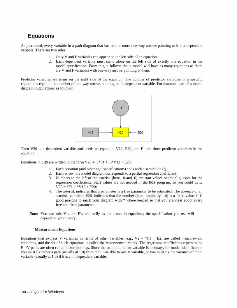
190 — EQS 6 for Windows
Equations As just noted, every variable in a path diagram that has one or more one-way arrows pointing at it is a dependent variable. There are two rules:
1. Only V and F variables can appear on the left side of an equation. 2. Each dependent variable must stand alone on the left side of exactly one equation in the
model specification. From this, it follows that a model will have as many equations as there are V and F variables with one-way arrows pointing at them.
Predictor variables are terms on the right side of the equation. The number of predictor variables in a specific equation is equal to the number of one-way arrows pointing at the dependent variable. For example, part of a model diagram might appear as follows:
Then V20 is a dependent variable and needs an equation. V12, E20, and F1 are three predictor variables in the equation. Equations in EQS are written in the form V20 = .8*F1 + .6*V12 + E20;
1. Each equation (and other EQS specifications) ends with a semicolon (;). 2. Each arrow in a model diagram corresponds to a partial regression coefficient. 3. Numbers to the left of the asterisk (here, .8 and .6) are start values or initial guesses for the
regression coefficients. Start values are not needed in the EQS program, so you could write V20 = *F1 + *V12 + E20;
4. The asterisk indicates that a parameter is a free parameter to be estimated. The absence of an asterisk, as before E20, indicates that the number (here, implicitly 1.0) is a fixed value. It is good practice to mark your diagram with * where needed so that you are clear about every free and fixed parameter.
Note: You can mix V’s and F’s arbitrarily as predictors in equations; the specification you use will
depend on your theory.
Measurement Equations Equations that express V variables in terms of other variables, e.g., V2 = *F1 + E2; are called measurement equations, and the set of such equations is called the measurement model. The regression coefficients representing F→V paths are often called factor loadings. Since the scale of a latent variable is arbitrary, for model identification you must fix either a path (usually at 1.0) from the F variable to one V variable, or you must fix the variance of the F variable (usually at 1.0) if it is an independent variable.

EQS 6 for Windows — 191
Construct Equations Equations for dependent F variables, such as F2 = *F3 + *V1 + D2; are called construct equations in EQS, because factors are sometimes called latent constructs.
Residuals in Regression Equations E- and D-type variables are residuals in regression equations. Whenever you write an equation for a dependent variable, you must be sure that it contains a residual as a predictor of that variable. You could arbitrarily assign E and D variables. However, E-type or error residuals are usually attached to V variables in equations using the same numbers, e.g., V7 = *F2 + E7;. The D-type or disturbance residuals are similarly attached to factors, e.g., F3 = .5*F2 + D3;. The variance of a residual variable is the unexplained variance in the dependent variable.
Bentler-Weeks Model Internally, EQS uses the matrix equations of the Bentler-Weeks structural equation system to represent models and their mean and covariance structures24. You do not deal with these matrix equations directly. However, since model specification is done in such a way that the program can set up the Bentler-Weeks model internally, you should know a few basic facts about the Bentler-Weeks approach. Any model setup will consist of equations, variances, and possibly covariances because of the following basic idea.
Parameters The parameters of any linear structural equation model are the regression coefficients in equations and the variances and covariances of independent variables. Equations were already illustrated above. Every dependent variable will have an equation, and each asterisk in each equation is a free parameter, a regression coefficient, to be estimated. Equations are collected in a section titled, appropriately enough, /EQUATIONS. Every independent variable must have a variance; each of these variances is a parameter. These variance parameters are often not explicitly shown in the path diagram, but they should be included in the model specification. Variances are given in the /VARIANCES section of the program, and are stated in a form as V1 = .5*; where, again, the number to the left of the * is the start value (which need not be given) and * indicates that the variance is a free parameter. If a variance parameter is to be fixed, as in F3 = 1.0; do not use *. Sometimes variances of factors are fixed for identification purposes. Residual E and D variables are always independent variables, so their variances will also need to be stated. V and F variables can be dependent or independent variables, depending on the model. Dependent variables cannot have variances that are parameters of the model. As in regression, the variance of a dependent variable is explained by the behavior of its predictors (which in turn may depend on other variables via additional equations) and the residual. Covariances of independent variables also are parameters if there are two-way arrows connecting independent variables in the path diagram.
Note: The covariance of a dependent variable with another variable cannot be a parameter! But a
dependent variable will have an associated residual, which is an independent variable that can carry such covariance information if needed.
24 Bentler, P. M., & Weeks, D. G. (1980). Linear structural equations with latent variables. Psychometrika, 45, 289-308.

192 — EQS 6 for Windows
Covariances are specified in the program in the /COVARIANCES section, using a “double-label” designation, e.g., the V1-V3 covariance has the designation V1,V3 as if it is the off-diagonal element of a matrix (which it is, internally). Here are some examples: V1,V3 = .5*; F3,F5 = *; V6, E3 = *;. Any pair of independent variables may covary, as long as the model is identified. This basic approach to the specification of models, via equations, variances, and covariances, covers all linear structural models, including regression, path analysis, simultaneous equations, confirmatory factor analysis, LISREL-type models, and so on. This simplicity and generality is a fundamental advantage of EQS.
Structured Means When you specify a model that contains structured means, your path diagram will contain a constant “variable” with arrows emanating from that constant to other variables in the model. For example, in the equation y = α + βx + ε, α is the intercept. The constant 1 is implicit, because we can rewrite the equation as y = α1 + βx + ε, thinking of the constant as a variable. This equation can be diagrammed as
where the path 1→y is the coefficient α, and the path y←x is the coefficient β. As usual, the diagram will be translated into equations, variances, and covariances, but interpretation of some parameters will be different. You should know a few additional concepts.
1. The parameters of the model include not only regression coefficients and variances and covariances of independent variables, but also the intercepts of the dependent variables and the means of independent variables. Thus in the example, α and µx (the mean of x) are also parameters.
2. An independent variable with a mean is treated as a dependent variable in EQS. In the example, x is an independent variable. But the model is modified to
since the equation x = µx1 + xd is added. The path 1→x represents µx,and xd is the deviation-from-mean variable. Thus x is now a dependent variable. The constant 1 is called V999 in EQS, and equations containing it are in the form V1 = 8*V999 + E1;.
3. The coefficient for regression on a constant is an intercept. Thus, in the equation F1 = *V999 + D1; the * regression coefficient is an intercept for factor 1.
4. The constant V999 is always taken as an independent variable that has no variance and no covariances with other variables in a model.

EQS 6 for Windows — 193
All of the ideas summarized above, plus additional modeling concepts, are spelled out in greater detail in the EQS 6 Structural Equations Program Manual.
Data File Preparation You should not immediately start modeling your data unless you have given some preliminary thought to the sequence of models that you might consider beyond your first model. The easiest and most efficient way to use EQS 6 for Windows is to have a manageable dataset in which you plan to use all or nearly all of the variables. If you have a large, cumbersome dataset from which you will select just a small subset of variables for analyses, you will force the program to search the large file with each run, thus wasting a lot of your own time. Surveys can have hundreds of variables, and working with such large files is a bad idea if you are going to be using 20 or fewer variables. Thus, we strongly suggest that you create for yourself a tidy little subset of the variables that will contain all of the variables that you are likely to be using in the entire sequence of models. The rest of the data should be set aside. If you decide to add some more variables from your big dataset later on, you can easily do so by using the Join feature of EQS 6 for Windows (see Chapter 3).
Variable Selection If you have a file with a large number of variables and want to cut this file down to manageable size, you can use what you know about the data to do logical, a priori variable reduction, eliminating redundant variables or those not relevant to your specific model. Alternatively, you may reduce your data by creating new composite variables that are sums of previously separate variables. Even after you create composite variables, however, you may have too many variables to use in a model. Then a procedure such as factor analysis may help you to select variables. We will discuss these various approaches to variable selection, but also will describe a situation in which you may want to create more, rather than fewer, variables.
A Priori Selection of Variables The selection of variables was described in Chapter 3, but we repeat some of the essential details here. We assume that you have imported your data into EQS, so that the file has the *.ess extension. Open your large *.ess file now, so that it becomes the active window. Click on Save As in the File option list.
Very Important Note: When the Save As dialog box appears, give a NEW name to the new, smaller file you will be saving. Otherwise, the smaller file will replace the large file, and the latter will be lost.
After you enter the new file name in the Save As dialog box, confirm that the Save File as Type field shows EQS System File. Click on Save to save this new file. You will see the Save Selected Cases or Variables dialog box.

194 — EQS 6 for Windows
Figure 7.1 Save Selected Cases or Variables Dialog Box
In this dialog box, you will see two list boxes side by side. The list box on the left is Variable list and the one on the right is Variables to save. By default, EQS saves all variables. If you want to change the default, you can use the four arrow buttons located between the two list boxes to move variables. The double-arrow buttons will move all variables from one list box to the other, whether or not any variables are selected. The single-arrow buttons only move those selected variables.
When you are finished choosing variables, click OK. EQS 6 for Windows will save your new, smaller file. When you are ready to start using the new file, close the original data file. Then use the Open option of the File menu to open the smaller file. Remember that, when you create your model, the measured variable names V1, V2, and so on, must correspond to the sequence of variables in your new file, that is, in the file you are actually using when you run EQS. If you are using a cut-down set as described above, you should make a record of the corresponding new numbers. For instance, you may have saved only variables V2, V4, V6, V8 and V10 from a larger file. In the cut-down file, they will be numbered V1, V2, V3, V4, V5, respectively. You should also update the labels. This updating will be done automatically if you do all your work within EQS 6 for Windows, since the labels are attached to variables in your *.ess files. But if you work with other types of files, you will have to do this updating yourself.
Creating New Composite Variables There are times when it is difficult to decide which of several variables to eliminate; yet you know that you cannot use all of the variables. For example, you may have a dozen attitude variables. However, because of the overall size of the model, you may want to use only three of these variables as indicators of a factor. Which variables should you keep, and which ones should you eliminate? You can use factor analysis to help you decide, as we note below. However, another approach is to keep all of the variables, and to combine them in new ways to produce a composite variable. A composite variable is a weighted sum of other variables.
Creating composites can raise issues, such as the fidelity of any model structure of the composites to the model structure of the original variables. A review of the issues is given in Bandalos and Finney (2001).25 A technical proof of equivalence under some circumstances is given by Yuan, Bentler, and Kano (1997).26
25 Bandalos, D. L., & Finney, S. J. (2001). Item parceling issues in structural equation modeling. In G. A. Marcoulides & R. E. Schumacker (Eds.) New Developments and Techniques in Structural Equation Modeling (pp. 269-296). Mahwah, NJ: Erlbaum. 26 Yuan, K.-H., Bentler, P. M., & Kano, Y. (1997). On averaging variables in a factor analysis model. Behaviormetrika, 24, 71-83.

EQS 6 for Windows — 195
There are two major ways to create a composite variable: matched composites, and homogeneous composites, see, e.g., Kishton and Widaman (1994).27
Matched Composites Without taking a stand on whether your variables are one-dimensional or multidimensional, you can create matched composites that should behave similarly. Such composites would have similar means and correlate similarly with other variables. You would assign variables to groups that are logically equivalent in terms of your knowledge of the total set of variables. If your 12 variables deal with two content domains, you could create two composite scores in which each composite contains items from both content domains. If the variables deal with four content domains, you would assign items so that each composite covers the four content domains. In the absence of content domain knowledge, you could assign variables to composites systematically. Here are two examples:
1. To create three indicator variables from 12 in a file, take V1, V4, V7, and V10 and add the raw scores of these variables to create one new variable. Then add the scores on V2, V5, V8, and V11 to create a second composite variable. Finally, add V3, V6, V9, and V12 to create the third composite variable.
2. You can create your new variables by randomly assigning variables to one of the several new composites.
In the matched composite approach, there is no reason to expect any one of the composites you create to be different from another. Each new composite should measure the same construct, or combination of constructs, as measured by a single composite of all original scores. The only exceptions would be for unanticipated content variation among variables, and the lower reliability of composites based on fewer variables.
Homogeneous Composites If there is some systematic variation in content among the variables, you could also create the composite variables by combining variables having similar content. So if your 12 variables represent facets of intelligence, and some of the variables stress verbal ability, while others stress quantitative ability, and still others stress spatial visualization, you could add the verbal scores to create a new verbal composite. Similarly, you can create composites for quantitative ability and spatial visualization. In contrast to the previous approach, the new composites may correlate quite differently with other variables. For example, the quantitative score may correlate more highly than the verbal score with success in engineering. When you take these new composites as indicators of a single construct, you can consider the latent variable to be a second-order factor that is based on the first-order factors of verbal, quantitative, and spatial intelligence. Of course, when you actually run a model based on only the three composite indicators, the factor would appear as a first-order factor. However, because of the content variation among indicators, you may want to consider whether nonstandard paths are appropriate. See the section Nonstandard Models in the EQS manual.
Direction of Scoring and Weighting However you decide to create new composite variables, you should remember that, when you combine variables, you must take the direction of scoring into account before you add scores. For example, a high score on one variable may indicate a positive attitude, but a high score on another variable may indicate a negative attitude. If you were simply to add two such variables, a person with a positive attitude would wind up in the middle of the continuum.
27 Kishton, J. M., & Widaman, K. F. (1994). Unidimensional versus domain representative parceling of questionnaire items: An empirical example. Educational & Psychological Measurement, 54, 757-765.

196 — EQS 6 for Windows
There are several ways to deal with this problem:
1. You can re-score one of the variables. For example, you could use the Reverse option of the Data menu to reverse the scoring of a 7-point V2 so that 1 ↔ 7, 2 ↔ 6, 3 ↔ 5.
2. You can change the sign of one of the variables before adding them. For example, use Data, Transformation, and choose Sign as the Function to transform the variable.
3. Instead of re-keying, you could simply use the Transformation option of the Data menu to create V1 - V2. This is, of course, the same as adding V1 + (-V2), i.e., changing the sign on the variable that needs re-keying. But this has the same effect as re-keying as far as variances and correlations are concerned.
Variable Transformations In general, you must use Data from the main menu, and Transformation, to create new variables based on linear or nonlinear transformations of existing variables. You must decide whether you want the variables to be weighted differently when creating your composite. In general, in the absence of knowledge about optimal scoring based on a previous use of a formal methodology, we suggest that you use equal weights with an appropriate sign, i.e., ±1 weights. However, if you want unequal weights, the EQS 6 for Windows transformation procedure permits you to create an unequally weighted composite variable such as V1 + .5*V2 - .3*V3. You should be sure that such a weighting is well justified.
Avoiding Linear Dependencies When you create a new composite variable, you should be sure that your final data file does not include both the original variables and a composite made up of a weighted sum of the original variables. To illustrate, you should not use a new file that contains V1 and V4, where V4 = V1 + V2 + V3. There will be an artificial dependency among such variables, and your correlation and covariance matrices cannot be used in structural modeling.
Using Factor Analysis to Select Variables When the variables in a data file are items on a questionnaire, it is usually desirable to add several items together to create a composite variable as described above. The new variables are more reliable and cover a wider range of substantive content than any single item could cover. But there may be times when the variables in your file have an intrinsic meaning. For example, a particular variable might be the Stanford-Binet Intelligence Test, a well-known standardized test. Then you may want to keep this particular variable in your model, if it is a good indicator of an IQ factor that you are studying. If you did a factor analysis of a lot of variables, including many that were reputedly alternative indicators of IQ, you might want to select those variables for your final model that are the best indicators of IQ. That is, you would select variables based on their factor loadings, on an IQ factor, obtained from an exploratory factor analysis. The procedures for doing an exploratory factor analysis have been discussed in Chapter 6. When you need to discover the factor structure for a large number of variables, you will want to do several factor analyses prior to getting ready for any structural modeling. But when you need only minor adjustments to your choice of indicators, you can use exploratory factor analysis to select variables for direct incorporation into a model setup. A method of doing this is discussed below.

EQS 6 for Windows — 197
Disaggregating Variables There may be times when you should do the very opposite of creating new composite variables. Rather, you should consider taking an existing variable in your data file and disaggregating it, taking it apart into its components. Consider, for example, that you want to create a latent variable model for the predictors and consequences of depression. Unfortunately, you have only one depression score in your data file. It would seem that you are relegated to doing a measured variable path model for this part of your model. Not true! It is possible that your depression variable actually is a composite of a set of items. For example, it might be a total score computed across 20 or 60 specific item responses of your subjects. Then you can create multiple indicators of a depression factor by going back to your original study and disaggregating the total score. Instead of creating one total score, you can create, say, two, three, or four. To create two composites, you could use the matched or homogenous approaches described above, depending on your purpose. For example, you could add the odd items (properly scored positive or negative, depending on the content direction) to get one new score, and add the even items to create another score. It may be necessary to do this disaggregating by hand, for example, by re-scoring items using another scoring template. It cannot be accomplished within EQS 6 for Windows, unless you happen to have a dataset that contains the original item responses. Then, of course, you can use the data transformation procedure discussed previously to create your new composites.
Case Selection In any modeling situation, you must be sure that the model is relevant to the sample of subjects at hand. For example, a model may be appropriate for males, but not for females. Using case selection to accomplish separation of your file into meaningful constituent files was discussed in Chapter 3. We do not want to repeat that discussion, but it is important to recognize applications for splitting a file, and for deleting an outlier case from the data file prior to using the Build_EQS procedure. One of the perennial problems in structural modeling is that one’s a priori model is liable to be inadequate to explain all variation and covariation in the data. Hence you may be enticed to do post hoc model modification with Lagrange Multiplier and Wald tests. A serious problem with this procedure is that it leads you to capitalize on chance associations in your data, making your model look better than it actually is. If your data file contains enough subjects, why not randomly split your sample into two separate samples? You can build the model using as much ad hoc model modification as you like. Then, use the second sample to cross-validate the results. The statistical tests you will get in sample 2 will not be biased by the model modification you did in sample 1. To select cases, bring up your current data file to the active window. Go to Data in the main menu, and click on the option Use Data. You will see the dialog box called Case Selection Specification.
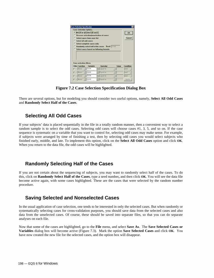
198 — EQS 6 for Windows
Figure 7.2 Case Selection Specification Dialog Box There are several options, but for modeling you should consider two useful options, namely, Select All Odd Cases and Randomly Select Half of the Cases.
Selecting All Odd Cases If your subjects’ data is placed sequentially in the file in a totally random manner, then a convenient way to select a random sample is to select the odd cases. Selecting odd cases will choose cases #1, 3, 5, and so on. If the case sequence is systematic on a variable that you want to control for, selecting odd cases may make sense. For example, if subjects were arranged by time of finishing a test, then by selecting odd cases you would select subjects who finished early, middle, and late. To implement this option, click on the Select All Odd Cases option and click OK. When you return to the data file, the odd cases will be highlighted.
Randomly Selecting Half of the Cases If you are not certain about the sequencing of subjects, you may want to randomly select half of the cases. To do this, click on Randomly Select Half of the Cases, type a seed number, and then click OK. You will see the data file become active again, with some cases highlighted. These are the cases that were selected by the random number procedure.
Saving Selected and Nonselected Cases In the usual application of case selection, one tends to be interested in only the selected cases. But when randomly or systematically selecting cases for cross-validation purposes, you should save data from the selected cases and also data from the unselected cases. Of course, these should be saved into separate files, so that you can do separate analyses on each file. Now that some of the cases are highlighted, go to the File menu, and select Save As. The Save Selected Cases or Variables dialog box will become active (Figure 7.3). Mark the option Save Selected Cases and click OK. You have now created the new file for the selected cases, and the option box will disappear.

EQS 6 for Windows — 199
Figure 7.3 Save Selected Cases or Variables Dialog Box The Save As file dialog box appears subsequently. Enter the new file name for the selected cases and make it an EQS System File. Figure 7.4 shows the Save As dialog box with the new file name, airsel.ess. Click on Save.
Figure 7.4 Save As Dialog Box
The original file with the highlighted cases will be closed, and the newly-saved file, airsel.ess, will be displayed on your screen. Repeat the File → Open airpoll.ess, Data → Use Data, and the previous selection and saving process, but this time you should save the unselected cases in their own file. Go to File again, and click on Save As. Give the new file name for these unselected cases, choose EQS System File and click Save. This time, mark the option Save Not-Selected Cases and click OK. You can close this file. For safety’s sake, you may want to bring up the two newly created files to verify that they contain the data that you expect to see there. Remember that you can use Data from the main menu, and then Information to get a quick summary of the number of cases in the new file. Between them, the new files should contain all cases from the original file.
Creating the File Manul7a.ess: Deleting an Outlier Case The file at hand must contain the logically relevant subjects. Also, it may be necessary to eliminate some cases because they are clearly not representative of the population characterized by the sample. We know that there is a problem with case #50 in the file manul7.ess. This outlier case creates havoc in the correlations and the factor structure of these (six variable, two factor) data. You can see the problem by plotting V1 against V3, or running a factor analysis on data containing case #50, and again on data without that case.

200 — EQS 6 for Windows
One way to handle outliers is to examine the output for the case’s contribution to Mardia’s coefficient of normalized multivariate kurtosis. Then, if the contribution is large, use the DELETE=50; statement in the /SPECIFICATION section of the model setup to eliminate the case. On the other hand, if you will be doing a variety of analyses with a file, and some of these methods do not have easy ways of dealing with outliers, you should probably create a file that has been purged of the offending cases. For instance, the factor analysis procedure available under Analysis does not have a simple method for deleting cases. You can create a new file, manul7a.ess, which does not contain case #50. You can do it yourself by applying what you learned in Chapter 3, or you can follow one of the methods below.
1. Open the manul7.ess file. Click on the missing data icon. The Missing Data Specifications dialog box will appear. Click the check box Display Univariate Outlier and click OK.
The Missing Data Pattern diagram of the data matrix will appear. The diagram will show no
missing data but will show that one case is an outlier on several variables. You can see that it is case 50. Choose Compute on the main menu, and select Mark Outliers. Click OK when you see Selected cases are marked in data sheet.
You will be taken back to the Missing Data Pattern plot. Close the plot and you will see the
manul7.ess file. If you use the vertical scroll bar to get to the end of the file, you will see that case #50 has been highlighted in black. Now you can go to File, click on Save As. In the Save As dialog box, give the name manul7a.ess, click on EQS System File and click on Save.
The Save Selected Cases or Variables dialog box will appear, and you should click on the button
to Save Not-Selected Cases. Then click OK. Your new file has now been created. You can close manul7.ess and bring up manul7a.ess to check, if you like.
2. Use the Edit procedures. Again, open the manul7.ess file. Use the vertical scroll bar to go to the
end of the file. Click on the case number for case 50. Case number 50 will be highlighted. Click on Edit from the main menu, and then Delete Rows. The case will disappear from the file. Now go to File, and click on Save As. Follow the instructions above, but instead of Save Not-Selected Cases in the Save Selected Cases or Variables dialog box, accept the default, namely Save All Cases.
3. Use the Select Cases procedure. There are several alternatives, outlined in Chapter 3. We discuss
the one based on Figure 3.23. In short, you invoke Data, then Use Data, to Select Cases Based on the Following Formula. The formula you use is V1 < 9. That will select and highlight all cases except #50. Use Save As to give the new file name, manul7a.ess, and Save Selected Cases. The new file will have 49 cases and six variables. Bring up this file so that you can work on it.
Data Plotting and Missing Values Before you embark on modeling, you should have explored your data using various plot and basic statistics features to assure yourself that the data are ready to be modeled. There is no point to modeling a dataset that contains missing values, outlier cases, or other anomalies unless you use one of the EQS options that control these problems. You should be sure that the missing value in your data file is properly defined. EQS allows two missing values for each variable. One is the system-wide missing value shared by all variables. It is usually used to mark the “blank field” in a questionnaire. It is displayed as a blank cell in an EQS data sheet. In addition to this system-wide missing value, you can define another missing value specifically for each variable. When the missing value is properly defined, EQS will skip cases with missing cells by default. However, EQS also provides a number of ways of imputing your data. These methods include mean and/or group mean replacement, fill-in by regression estimators, and replacement of missing cells using EM estimators. Alternatively, you can compute correlations and covariances based on available data for reading into the EQS model file. If for some reason you have not already dealt with this issue, do it now before you go on to do further analyses. Of course, if you use the special missing data or case-robust methodology for modeling described later, this preprocessing is not necessary.
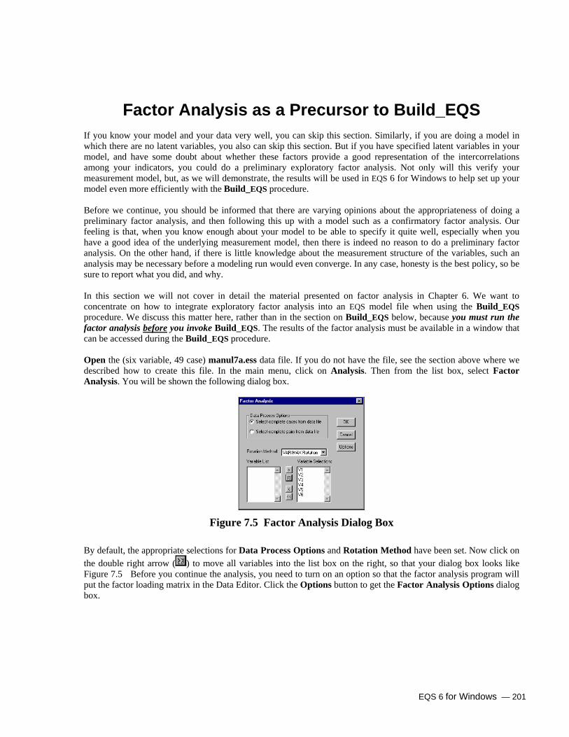
EQS 6 for Windows — 201
Factor Analysis as a Precursor to Build_EQS If you know your model and your data very well, you can skip this section. Similarly, if you are doing a model in which there are no latent variables, you also can skip this section. But if you have specified latent variables in your model, and have some doubt about whether these factors provide a good representation of the intercorrelations among your indicators, you could do a preliminary exploratory factor analysis. Not only will this verify your measurement model, but, as we will demonstrate, the results will be used in EQS 6 for Windows to help set up your model even more efficiently with the Build_EQS procedure. Before we continue, you should be informed that there are varying opinions about the appropriateness of doing a preliminary factor analysis, and then following this up with a model such as a confirmatory factor analysis. Our feeling is that, when you know enough about your model to be able to specify it quite well, especially when you have a good idea of the underlying measurement model, then there is indeed no reason to do a preliminary factor analysis. On the other hand, if there is little knowledge about the measurement structure of the variables, such an analysis may be necessary before a modeling run would even converge. In any case, honesty is the best policy, so be sure to report what you did, and why. In this section we will not cover in detail the material presented on factor analysis in Chapter 6. We want to concentrate on how to integrate exploratory factor analysis into an EQS model file when using the Build_EQS procedure. We discuss this matter here, rather than in the section on Build_EQS below, because you must run the factor analysis before you invoke Build_EQS. The results of the factor analysis must be available in a window that can be accessed during the Build_EQS procedure. Open the (six variable, 49 case) manul7a.ess data file. If you do not have the file, see the section above where we described how to create this file. In the main menu, click on Analysis. Then from the list box, select Factor Analysis. You will be shown the following dialog box.
Figure 7.5 Factor Analysis Dialog Box
By default, the appropriate selections for Data Process Options and Rotation Method have been set. Now click on the double right arrow ( ) to move all variables into the list box on the right, so that your dialog box looks like Figure 7.5 Before you continue the analysis, you need to turn on an option so that the factor analysis program will put the factor loading matrix in the Data Editor. Click the Options button to get the Factor Analysis Options dialog box.

202 — EQS 6 for Windows
Figure 7.6 Factor Analysis Options Dialog Box
There are a number of useful options in this dialog box. Click on the check box next to Put factor loading matrix in a data editor, so that your dialog box looks like Figure 7.6 . Click the OK button after the selection is made. Almost immediately, you will get a plot of the eigenvalues of the correlation matrix (Y Axis) against the component number (X Axis).
Figure 7.7 Plot of Eigenvalues
The dotted-red horizontal line represents the cutoff for eigenvalues to use (by default, 1.0). The first two eigenvalues are clearly greater than 1.0. In fact, the eigenvalues are 2.339, 1.415, and .775 in sequence, as you would see if you went to Window and selected the output.log for the numbers. As indicated by the number of eigenvalues above the dotted line, the choice of two factors seems to be appropriate, since there is a good-sized gap between the 2nd and 3rd eigenvalues. Also, the remaining eigenvalues, under the line, form an approximately straight line. This line is often called the “scree” line. Some researchers urge selection of the number of factors by the scree test, keeping the eigenvalues above the scree line. In any case, since there should be at least 3 good indicators per factor, when you have 6 variables, you should be satisfied with 2 factors. To start the factor analysis, click on the Work menu and select Factor Specifications in the menu bar. The Factor Analysis Selection Box shown in Figure 7.8 will appear.

EQS 6 for Windows — 203
Figure 7.8 Factor Analysis Selection Box
This box allows you to change the number of factors, or modify the cutoff eigenvalue criterion for determining the number of factors. Accept the default by clicking OK. The program will do the factor analysis. Almost immediately, you will see an information box telling you that the factor analysis is done. Click OK. You will see the newly created file called factor2.ess as the active window.
Figure 7.9 Factor Loading Matrix in Data Editor This file name is picked by default. Whenever a factor analysis is sent to the Data Editor, a factor?.ess file will be created, where ? will be replaced by the number of factors in the run (here, 2). This file, shown in Figure 7.9, gives the factor loading matrix resulting from an orthogonal rotation (VARIMAX by default) of the initial factor analysis solution. If you preferred a different solution, you could have selected it in the Rotation Method box in the middle of Figure 7.5 .
From the factor loading matrix shown in Figure 7.9, we can decide which variables are good indicators of each factor. Here, variables V1-V3 are good marker variables for factor 1, while variables V4-V6 provide good marker variables for factor 2. That same conclusion can be obtained automatically; see Figure 7.13, below. (Remember that the signs of all variables in a column of a factor loading matrix are arbitrary. They can be reversed, since a sign only determines how you interpret the meaning of a high score on the factor.) In this analysis, it is quite certain that we want exactly two factors. In your own analyses, you may not be sure whether you have the best solution until you try factor solutions with a varying number of factors. Each of these can be sent to the data editor, in a factor?.ess file.
Note: If you repeat a run with a given number of factors, say two, the new factor2.ess file will overwrite
the old one. In general, you should not use the name factor?.ess for your own files because factor runs always will use these file names.

204 — EQS 6 for Windows
You can keep track of the results obtained from the factor2.ess file by yourself, perhaps with written notes, to use when setting up the EQS model file. But we shall show below how to automatically import this information into the model file setup.
Build a two-factor CFA model In this section, we will show you how to build an EQS model by using the results from factor analysis. The results of factor analysis from the previous section suggest that the dataset will support a two-factor model. In that analysis, variables V1 to V3 will load on one factor and variables V4 to V6 will load on another factor. We hypothesize that a two-factor factor analytic model be tested for this data. This kind of model is called Confirmatory Factor Analytic or a CFA model.
We continue from Figure 7.9. Click OK in the information box which asks “Return to data file?” EQS will return you to manul7a.ess. Then, in the main menu, click on Build_EQS and choose the Title/Specifications option. Build_EQS presents you with a series of dialog boxes for specifying your model. After you complete each dialog box, its information is transferred to a new file, temporarily called datafile.eqx, where the datafile is the name of your data. In this example, the default EQS model file name is manul7a.eqx. This file will be in the background for you to scan. You may also modify it, by using various dialog boxes, if you change your mind about any options. After the model is completely specified using the usual EQS conventions, this file is sent to the EQS 6 for Windows program to estimate parameters and yield model test results. The results from the modeling run are then placed into the output file, which is manul7a.out by default. Here is the outline for building a two-factor CFA model with an equation table:
1. After factor analysis is complete, bring up the manul7a.ess file from the Window menu. 2. Click on Build_EQS and Title/Specifications to get the EQS Model Specifications dialog
box. Click OK. 3. Click on Build_EQS → Equations to bring up the Build Equations dialog box. 4. Select the radio button labeled Adopt Equations from Factor Analysis. Click OK. 5. Complete the Create Equation and Create Variance/Covariance windows.
Title/Specifications The Title/Specifications option brings up the dialog box shown in Figure 7.10. Initially, the EQS Model Title edit box is filled with “EQS 6 for Windows” followed by the data file name. The default title is designed with a purpose. It tells you that the model is generated by EQS 6 and this model is based on manul7a.ess. In case you need to revisit the model months or even years later, you still can identify the program and dataset that generated it.
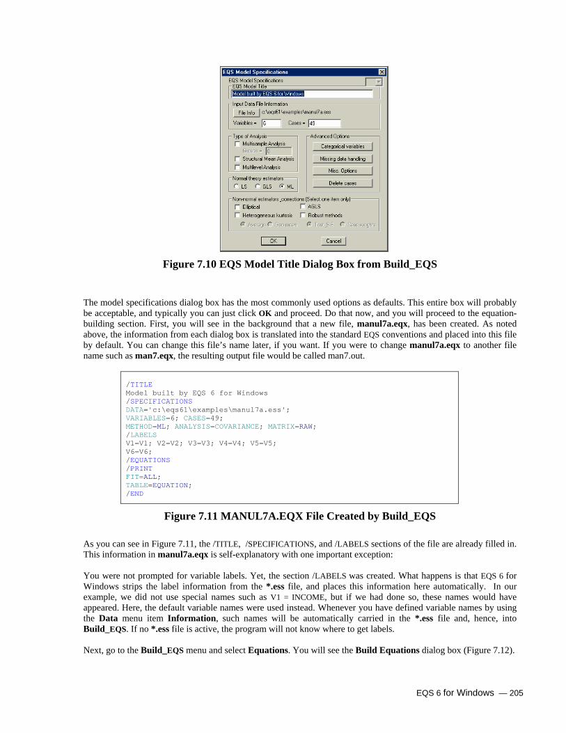
EQS 6 for Windows — 205
Figure 7.10 EQS Model Title Dialog Box from Build_EQS The model specifications dialog box has the most commonly used options as defaults. This entire box will probably be acceptable, and typically you can just click OK and proceed. Do that now, and you will proceed to the equation-building section. First, you will see in the background that a new file, manul7a.eqx, has been created. As noted above, the information from each dialog box is translated into the standard EQS conventions and placed into this file by default. You can change this file’s name later, if you want. If you were to change manul7a.eqx to another file name such as man7.eqx, the resulting output file would be called man7.out.
/TITLE Model built by EQS 6 for Windows /SPECIFICATIONS DATA='c:\eqs61\examples\manul7a.ess'; VARIABLES=6; CASES=49; METHOD=ML; ANALYSIS=COVARIANCE; MATRIX=RAW; /LABELS V1=V1; V2=V2; V3=V3; V4=V4; V5=V5; V6=V6; /EQUATIONS /PRINT FIT=ALL; TABLE=EQUATION; /END
Figure 7.11 MANUL7A.EQX File Created by Build_EQS As you can see in Figure 7.11, the /TITLE, /SPECIFICATIONS, and /LABELS sections of the file are already filled in. This information in manul7a.eqx is self-explanatory with one important exception: You were not prompted for variable labels. Yet, the section /LABELS was created. What happens is that EQS 6 for Windows strips the label information from the *.ess file, and places this information here automatically. In our example, we did not use special names such as V1 = INCOME, but if we had done so, these names would have appeared. Here, the default variable names were used instead. Whenever you have defined variable names by using the Data menu item Information, such names will be automatically carried in the *.ess file and, hence, into Build_EQS. If no *.ess file is active, the program will not know where to get labels. Next, go to the Build_EQS menu and select Equations. You will see the Build Equations dialog box (Figure 7.12).

206 — EQS 6 for Windows
Figure 7.12 Build Equations Dialog Box In our example, we shall use all variables. Click on the radio button for Adopt Equations From Factor Analysis, so that the dialog box looks like Figure 7.12. Then click OK; you immediately see Figure 7.13. If instead we had selected Create New Equations by clicking its radio button, and filled in the number of factors, we would have obtained Figure 7.13, but the columns for F1 and F2 would be blank.
Create Equation This dialog box contains one row for each possible equation. Variables V1 through V6 could be dependent, as could the two factors F1 and F2. Thus there could be a maximum of eight equations. In a factor analysis model, only Vs are dependent variables. In more general models, some Fs could also be dependent variables.
Figure 7.13 Create Equations Dialog Box
The columns list the possible predictors of each of the dependent variables. Predictor variables may be dependent or independent variables, depending on the model. In a factor analysis model, only Fs are predictors of the V variables, and the predictor Fs are all independent variables. Some cells of the matrix in Figure 7.13 have a 1 or an asterisk (*), while other cells do not. Each asterisk refers to a free parameter in the model. When you click on a cell in the matrix repeatedly, the asterisk will be shown, and then removed, then shown again. Hence by clicking, you can put an asterisk wherever you want, or remove it at will. The 1’s are fixed parameters; see Identification Issues, below. When you select Adopt Equations from Factor Analysis in the Build Equations dialog box (Figure 7.12), as we did, the elements of Create Equation are set automatically in accordance with the elements of the factor loading matrix (ours, in factor2.ess) that exceed the specified filter value (here, 0.5). So, in our example, Figure 7.13 was created automatically and we click OK to continue. If the results were not to our liking for any reason, we could edit the matrix further in the ways discussed, before clicking OK. When we click OK, the Create Variance/Covariance dialog box will appear (Figure 7.14).

EQS 6 for Windows — 207
Variances/Covariances The variances and covariances of independent variables are specified in the next dialog box. The independent variables now include residual E and D variables associated with V and F variables, if these are relevant to the model. As before, you must place an asterisk in each position that you want to represent as a free parameter. By default, as you can see, the diagonal elements of this matrix have the asterisk inserted in them. Thus by default, the variance of each of these variables is a free parameter. This may or may not be what you want to do. Also, by default, no covariances are specified. If you want some covariances, you will have to put asterisks in the relevant positions.
Figure 7.14 Create Variances/Covariances Dialog Box In the case of a confirmatory factor analysis model, it is typical practice to allow factors to correlate. So, in the example, click on the F2,F1 position. The * will appear, indicating a free parameter, and your dialog box will look like Figure 7.14. If you wanted to allow certain correlated errors, those would be specified here as well. But we are satisfied with the variance/covariance specification, so click OK. The resulting specifications will be transferred to the manul7a.eqx file. The complete model built by EQS’ Build_EQS facility is shown as follows:
/TITLE Model built by EQS 6 for Windows /SPECIFICATIONS DATA='c:\eqs61\examples\manul7a.ess'; VARIABLES=6; CASES=49; METHOD=ML; ANALYSIS=COVARIANCE; MATRIX=RAW; /LABELS V1=V1; V2=V2; V3=V3; V4=V4; V5=V5; V6=V6; /EQUATIONS V1 = 1F1 + E1; V2 = *F1 + E2; V3 = *F1 + E3; V4 = 1F2 + E4; V5 = *F2 + E5; V6 = *F2 + E6; /VARIANCES F1 = *; F2 = *; E1 = *; E2 = *; E3 = *; E4 = *; E5 = *; E6 = *; /COVARIANCES /PRINT FIT=ALL; TABLE=EQUATION;

208 — EQS 6 for Windows
/END
Figure 7.15 Complete EQS Model Created by the Equation Table
The six equations in the /EQUATIONS section above correspond to our specification in Figure 7.13. Note that the E residuals have been added, and each equation ends with a semicolon as required by the EQS program. The /VARIANCES and /COVARIANCES sections correspond to Figure 7.14. The variances of F1 and F2 are free variances. All error variances are free parameters, with no start value given, so EQS will pick its own start values. The only covariance specified is that between the factors. The model is complete at this point. To run it, go back to the Build_EQS menu and pull down the menu bar. Click on Run EQS, where you will be asked to save the model. You must save the model and EQS will proceed to run the model. When the job is done, the output file will be opened and displayed in front of you.
Asterisks and Free Parameters: Identification Issues Remember that you must fix the scale of each factor, by fixing a path from it or fixing its variance (only if it is an independent variable). In the above example, EQS 6 for Windows has done the work for you, by fixing the first coefficient of F1 and F2 at 1. Another way to do this is to request that EQS fix one coefficient and free others; see Figure through Figure , below. Still another way is to run the manul7a.eqx file, creating a model file manul7a.eqs, which can be edited. In that case, identification constraints will not be added automatically for you. You have to take care of them yourself.
Build a Two-factor CFA Model using /MODEL An alternative to Equation Table uses substantial shortcuts to build a model. These short cuts can be found in the newly added /MODEL section. Let’s assume that we have a priori knowledge on the two-factor CFA model we have just discussed. You can specify a model without equations, variances, and covariances. Please take a look at the following EQS model file:
/TITLE Two factor CFA model using /MODEL short cuts /SPECIFICATIONS DATA='c:\eqs61\examples\manul7a.ess'; VARIABLES=6; CASES=49; GROUPS=1; METHODS=ML; MATRIX=RAW; ANALYSIS=COVARIANCE; /LABELS V1=V1; V2=V2; V3=V3; V4=V4; V5=V5; V6=V6; /MODEL (V1 TO V3) ON F1; (V4 TO V6) ON F2; COV (F1,F2) = *; /PRINT FIT=ALL; /END
Figure 7.15 Two-Factor CFA Model
This model in some way is very similar to most models you have seen. It has the basic elements of /TITLE, /SPECIFICATIONS, and /LABELS. However, there is a /MODEL section, which replaces /EQUATIONS, /VARIANCES, and /COVARIANCES.

EQS 6 for Windows — 209
Let’s take a good look at the commands. The first factor structure is defined as:
(V1 TO V3) ON F1;
That is, V1 to V3 load on F1. Note that the “on” command can be expanded to more variables, simply by adding variables inside the parentheses, using commas to separate them. The next command defines the second factor structure. Another command is:
COV (F1,F2)=*;
This command defines the covariance between F1 and F2 as a free parameter whose start value will be determined by EQS. If more factors are inside the parentheses, EQS will define all the covariances among them to be free parameters.
You have a complete model and are ready to run the model. Go to Build_EQS menu and select Run EQS to run the model. Before any analysis is performed, EQS will first expand the commands in the /MODEL section. The expanded model is listed in the output file with /EQUATIONS, /VARIANCES, and /COVARIANCES as shown in Figure 7.15.
Then EQS will perform the analysis specified in the model and display the output when it is complete.
Build a Path Analysis Model The path analysis model is one of the models often tested. It is actually an ordinary multivariate regression model. The data file we are using is manul4.ess (Figure 7.17). It is a six-variable correlation matrix with standard deviations at the bottom of the matrix. The first two variables are ANOMIE and POWERLESSNESS measured in 1967. The same two variables are measured again in 1971, a so-called panel or longitudinal design. The last two variables are ignored for now. The model we are interested in is Figure 7.16. This is a cross-lagged panel design, which is also used to test more restrictive models regarding the relative influence of the cross-lagged variables on each other.
POWRLS67
ANOMIE71ANOMIE67
POWRLS71 E4
E3
Figure 7.16 Diagram for Cross-lag Panel Model
Figure 7.17 Manul4.ess for Cross-lag Panel Model

210 — EQS 6 for Windows
Here is the outline for building a path analysis model:
1. Open manul4.ess from the C:\EQS61\Examples folder. 2. Click on Build_EQS → Title/Specifications to get the EQS Model Specifications dialog
box. Click OK. 3. Click on Build_EQS → Equations to bring up the Build Equations dialog box. 4. Select the radio button labeled Create New Equations and enter 0 in the Number of Factors
edit box. Uncheck the Use All Variable check box. Click OK. 5. In the Select Variable to Build Equations dialog box, move the first four variables in
Variables in Equation list box. Click OK. 6. Complete Create Equation and Create Variance/Covariance windows.
We always recommend opening the dataset before a model is built. When you do that, Build_EQS will gather all necessary data information so that you don’t have to. So open manul4.ess on the screen before we start this model building process. Then click on Build_EQS and pull down its menu. You will see that only two menu items are available, Title/Specification and EQS working array. Click on Title/Specification and a dialog box will appear, as shown in Figure 7.18. There are many buttons and boxes in this dialog box. The title has been filled, input data file information shows a sample of six variables and 932 observations, and the estimation method is set at ML. All other buttons and boxes are irrelevant at this point so we ignore them. In other words, when building a standard model, much information is provided if you have an EQS data file (*.ess) file open.
Figure 7.18 Specification Dialog Box to Prepare a Path Analysis Model Since the input data information has been provided, you are ready to build the model. Click on the OK button in the EQS Model Specifications dialog box. You will see that a new window titled “manul4.eqx” is opened, containing some EQS commands. (Note that EQS took the name “manul4” from the name of the data file.) These EQS commands include /TITLE, /SPECIFICATIONS, and /LABELS.
Return to the Build_EQS menu. You will see that a few more menu items are activated. They are Equations, Reliability, and Run EQS. The model you are trying to build is incomplete; you cannot run it yet. Click on Equations to bring up the Build Equations dialog box (Figure 7.19) to specify your model. Notice that in this dialog box, the Create New Equations option is set. The dialog box also shows that there are six variables. You need to fill in zero in the Number of Factors edit box since we are building a path model. You also need to un-check Use All Variable so that you can select the variables to be included in the model. Now your dialog box looks like Figure 7.19, so click on OK. You will see the Select Variable to Build Equations dialog box as shown in Figure 7.20. Move the four variables to be used in the equations to the list box labeled Variables in Equation. Now your dialog box looks like Figure 7.20, so click on the OK button.

EQS 6 for Windows — 211
Figure 7.19 Build Equations Dialog Box
Figure 7.20 Select Variables Dialog Box
After you click on the OK button in the dialog box shown in Figure 7.20, you will be given an equation table to specify your model (Figure 7.21). In this Create Equation dialog box, you will see four variables, ANOMIE67, POWRLS67, ANOMIE71, and POWRLS71, listed both row-wise and column-wise. Each row represents a dependent variable and each column represents a predictor variable. You must fill in information in the cells to complete the model. Please note that we use asterisks for free parameters and numbers without asterisks as fixed parameters.
Figure 7.21 Path Analysis Model Create Equation Table
According to the diagram shown in Figure 7.16, the equations in this model will look like:
ANOMIE71 = *ANOMIE67 + *POWRLS67 + error; POWRLS71 = *ANOMIE67 + *POWRLS67 + error;
When you try to specify the equation table to create these two equations, you must fill the cells between the corner of (ANOMIE71, ANOMIE67) and (POWRLS71, POWRLS67) with asterisks. There are a total of four cells. How are you going to fill these cells easily?
Method 1: Fill one cell at a time. You can single-click the designated cells. For each click, an asterisk will appear, indicating that it is a free parameter. This is an easy way to specify free parameters but it could get very tedious when many parameters needed to be created.
Method 2: Fill many cells in one click.
Place your mouse pointer above and to the left of the rectangle you want to fill, click on the left mouse button and hold it down, slowly drag your mouse pointer down and to the right until the rubber rectangle has completely covered the cells you wish to fill, then release the mouse button. A Start Value Specifications dialog box will appear (Figure 7.22). In this box, you can select Regular free parameters, Fix one and free others, Intercept paths, Slope paths, and Remove parameters. The radio button is set at Fix one and free others by default. (You can change the default by going into Edit/Preferences.) Set the option to Regular
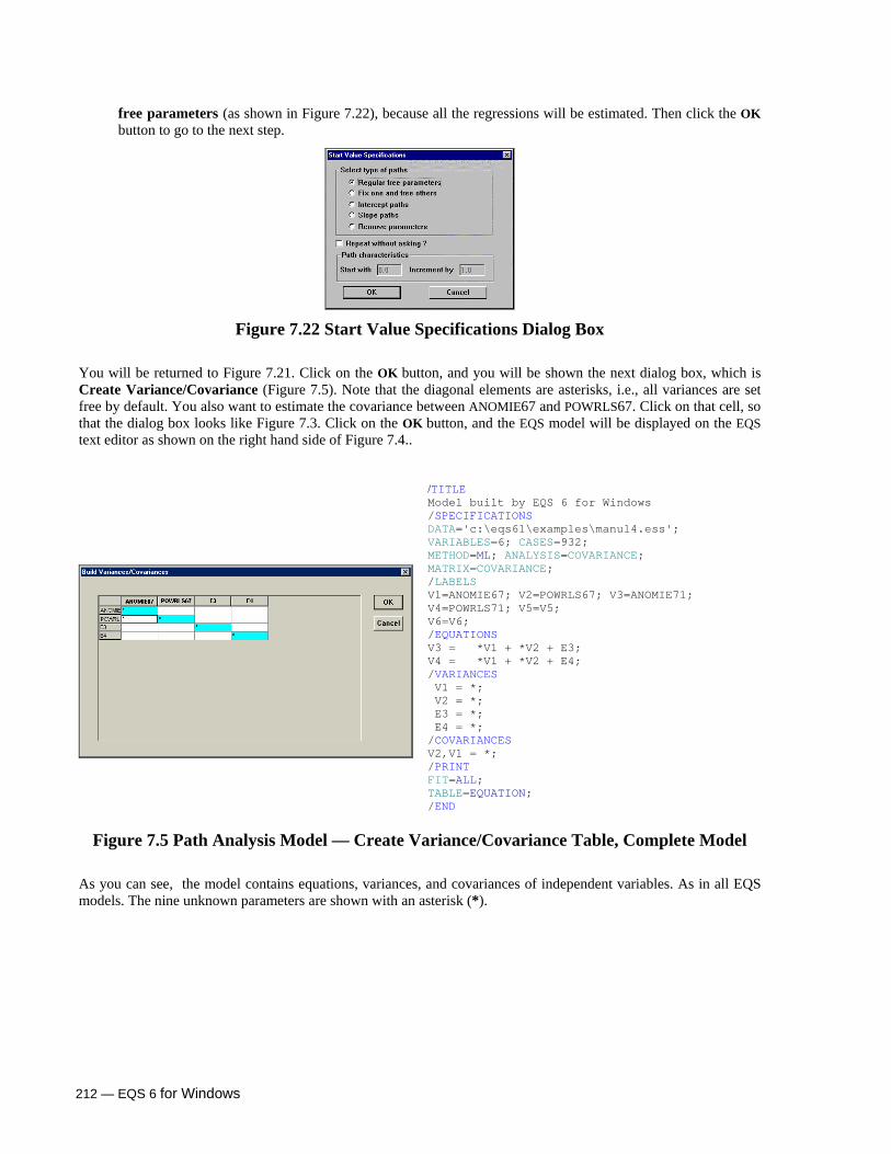
212 — EQS 6 for Windows
free parameters (as shown in Figure 7.22), because all the regressions will be estimated. Then click the OK button to go to the next step.
Figure 7.22 Start Value Specifications Dialog Box You will be returned to Figure 7.21. Click on the OK button, and you will be shown the next dialog box, which is Create Variance/Covariance (Figure 7.5). Note that the diagonal elements are asterisks, i.e., all variances are set free by default. You also want to estimate the covariance between ANOMIE67 and POWRLS67. Click on that cell, so that the dialog box looks like Figure 7.3. Click on the OK button, and the EQS model will be displayed on the EQS text editor as shown on the right hand side of Figure 7.4..
/TITLE Model built by EQS 6 for Windows /SPECIFICATIONS DATA='c:\eqs61\examples\manul4.ess'; VARIABLES=6; CASES=932; METHOD=ML; ANALYSIS=COVARIANCE; MATRIX=COVARIANCE; /LABELS V1=ANOMIE67; V2=POWRLS67; V3=ANOMIE71; V4=POWRLS71; V5=V5; V6=V6; /EQUATIONS V3 = *V1 + *V2 + E3; V4 = *V1 + *V2 + E4; /VARIANCES V1 = *; V2 = *; E3 = *; E4 = *; /COVARIANCES V2,V1 = *; /PRINT FIT=ALL; TABLE=EQUATION; /END
Figure 7.5 Path Analysis Model — Create Variance/Covariance Table, Complete Model
As you can see, the model contains equations, variances, and covariances of independent variables. As in all EQS models. The nine unknown parameters are shown with an asterisk (*).

EQS 6 for Windows — 213
Build a Latent Growth Curve Model McArdle (1988)28 and McArdle and Epstein (1987)29 reported a study using Wechsler Intelligence Scale for Children (WISC) scores for 204 children measured longitudinally between 1961 and 1965. The data consist of WISC scores collected at four time points, and mother’s education. Figure 7.24 is an illustration of this model. Figure 7.25 shows this data as a correlation matrix with standard deviations and means. The data were collected at unequal time intervals. The relative time intervals for data collection were 0, 1, 3, and 5, which values we could use for our slope parameters in a so-called initial status model. An alternative for the growth parameters is -2.25, -1.25, 0.75, and 2.75, obtained by subtracting the mean 2.25 from the initial status slopes, yielding slopes with mean zero, a so-called time-averaged model. In our illustration, we will use the time-averaged model as the example to build the model.
The diagram (Figure 7.24) discussed here is illustrated as follows:
D2
WISC_1
WISC_2
WISC_3
WISC_4
InterceptFactor
LinearGrowthFactor
E1
E2
E3
E4
Constant
D1
MOMEDUCE5
Figure 7.24 Latent Growth Model on WISC Data
Here is the outline of the process for creating a latent growth curve model.
1. Open wisc.ess from the C:\EQS61\Examples folder. 2. Click on Build_EQS -> Title/Specifications to get the EQS Model Specifications dialog
box. Check the check box labeled Structural Mean Analysis. Click OK. 3. Click on Build_EQS -> Equations to bring up the Build Equations dialog box. 4. Select the radio button labeled Create New Equation and enter 2 in the Number of Factors
edit box. Click OK.
28 McArdle, J. J. (1988). Dynamic but structural equation modeling of repeated measures data. In J. R. Nesselroade & R. B. Cattell (Eds), Handbook of Multivariate Experimental Psychology (pp. 561-614). New York: Plenum. 29 McArdle, J. J., & Epstein, D. (1987). Latent growth curves within developmental structural equation models. Child Development, 58, 110-133.

214 — EQS 6 for Windows
5. Complete Create Equation so that F1 is an intercept factor and F2 is a growth factor (see below). Edit the start values accordingly.
6. Complete Create Variance/Covariance window and specify covariances accordingly. Open the wisc.ess data (Figure 7.25), which you can find in the example folder of the EQS 6 folder. To build the model, pull down the Build_EQS menu and select Title/Specifications. The dialog box is shown in Figure 7.26.
Figure 7.25 Data for WISC Scores
Figure 7.26 EQS Model Specifications Dialog Box for Latent Growth Curve Model As shown previously, the dialog box is filled with the information from the dataset we are using. Namely, the data file name is wisc.ess and it has 5 variables with 204 observations. The default estimation method is ML. In most Latent Growth Curve models, the structured mean is an essential part of the model. This is no exception; we need to build a model with means. We need to turn on the Structural Mean Analysis option so that it is checked as in Figure 7.26.
Now Figure 7.26 has all the information we need to proceed to the next step. Click the OK button. The dialog will disappear, a new text window will be opened, and we will see some model information displayed on the screen. Please note that this listing includes two sections which are /STANDARD DEVIATION and /MEANS, and that the input matrix is a correlation matrix. The combination of input correlation matrix with standard deviation and mean sections instructs EQS to convert the input matrix to either a covariance matrix with means (if ANALYSIS=MOMENT, as in Figure 7.27) or a covariance matrix. All these conversions are done internally in EQS; there is no need for you to do anything extra.

EQS 6 for Windows — 215
/TITLE Model built by EQS 6 for Windows /SPECIFICATIONS DATA='c:\eqs61\examples\wisc.ess'; VARIABLES=5; CASES=204; METHOD=ML; ANALYSIS=MOMENT; MATRIX=COVARIANCE; /LABELS V1=WISC_1; V2=WISC_2; V3=WISC_3; V4=WISC_4; V5=MOMEDUC; /END
Figure 7.27 Partial EQS Commands for Latent Growth Curve Model With the partly-built EQS model on the screen, we need to return to Build_EQS and select Equation; a Build Equations dialog box will appear (Figure 7.28). As we can see, the dialog box makes Create New Equations its default option. The dialog box also specifies 5 indicator variables, and both the Structured Means and Use All Variable options are checked. We want to build a structured mean model with all five variables. The only information left unspecified is the number of factors. Since we know that we are going to build a linear growth model, there will be two factors in the model. One factor is the intercept factor and the other is the linear growth factor. We therefore enter 2 in the edit box labeled Number of Factors. Figure 7.28 shows a completed Build Equations dialog box.
Figure 7.28 Build Equations Dialog Box for Latent Growth Curve Model Click on the OK button in the Build Equations dialog box, and a Create Equation dialog box will appear (Figure 7.31). The dialog box has rows for each indicator variable, and columns for V999, F1, and F2, followed by indicator variables. Since we have decided that there are two factors, we must select intercept and growth factors. Let’s assume F1 is the intercept factor and F2 is the growth factor; we need to set the starting values of the intercept factor to fixed one.
Click the mouse on the cell labeled V999 and hold the mouse button, dragging it slowly down and to the right until the rubber rectangle completely covers the first four rows in the F1 column. Release the mouse button; you will see a Start Value Specifications dialog box (Figure 7.29). Select the Intercept paths option and change the starting value to 1.0 in the lower edit box. Your dialog box now looks like Figure 7.29, so click the OK button. In Figure 7.31, the starting values under F1 are now equal to 1.0. Similarly, drag a rubber rectangle over the first four rows in the F2 column, and turn on the Slope paths option. The starting values will become 0, 1, 2, and 3. Since we have decided that the starting values for the growth factor are -2.25, -1.25, 0.75 and 2.75 for the time-averaged model, you need to specify the starting values individually. To edit a cell in the equation table, you first must double-click the cell to make it editable. First, double-click the cell in the WISC_1 row and F2 column, and change the start value from 0 to -2.25. Press the ENTER or Tab key to make the change. Similarly, make the changes for WISC_2 to WISC_4 in the F2 column.

216 — EQS 6 for Windows
Figure 7.29 Intercept Start Values
Figure 7.30 Slope Start Values In addition to the factors, there is the mean variable (i.e., V999) to be considered in the latent growth curve model. This latent growth curve model will estimate the mean of mother’s education and the mean of the intercept and growth factors. After putting an asterisk in each of those three cells, click OK to get the complete equation table shown in Figure 7.31.
Figure 7.31 Create Equation Dialog Box
Note that the intercept and slope paths in this kind of model are fixed parameters, i.e., have no asterisk in Figure 7.31 Click the OK button to move the program to Create Variance/Covariance. EQS will make all error variances free parameters by default. The mean variable (V999) is a constant and is fixed at 1. To correlate the disturbances and error variance among D1 (for intercept factor), D2 (for linear growth factor), and E5 (for mother’s education), single-click in the cells for these three parameters. The complete specifications are shown in Figure 7.32.
Figure 7.32 Create Variance/Covariance Dialog Box
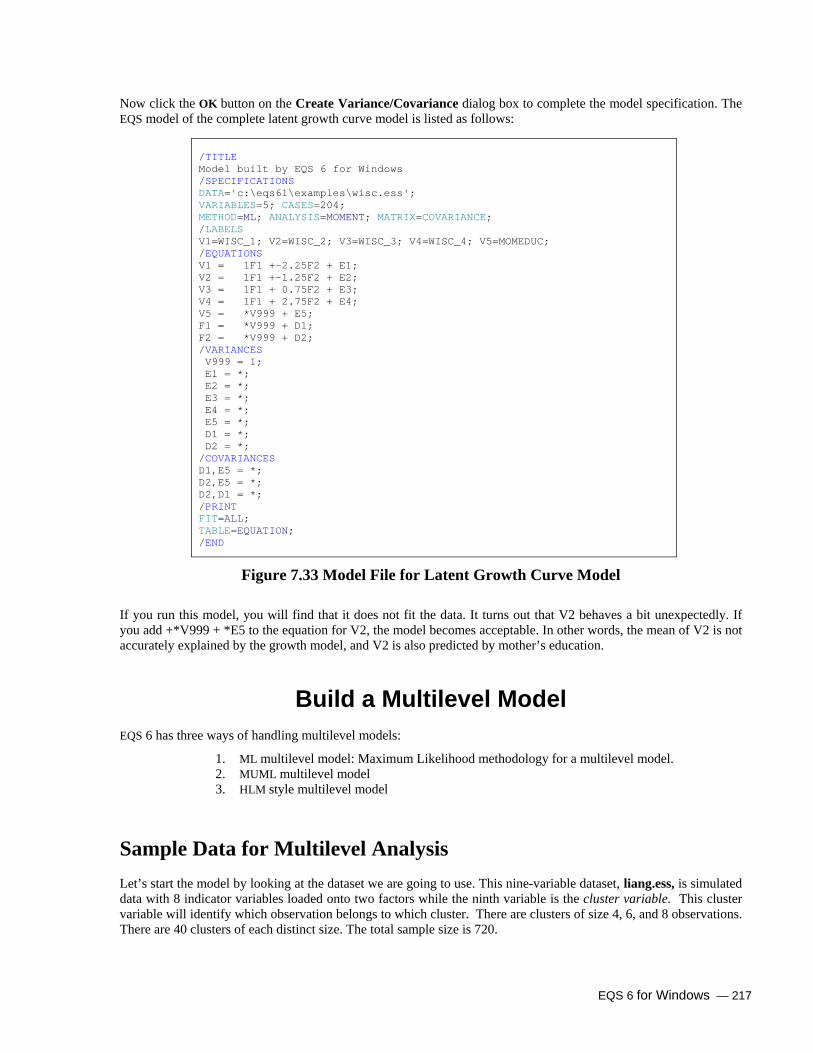
EQS 6 for Windows — 217
Now click the OK button on the Create Variance/Covariance dialog box to complete the model specification. The EQS model of the complete latent growth curve model is listed as follows:
/TITLE Model built by EQS 6 for Windows /SPECIFICATIONS DATA='c:\eqs61\examples\wisc.ess'; VARIABLES=5; CASES=204; METHOD=ML; ANALYSIS=MOMENT; MATRIX=COVARIANCE; /LABELS V1=WISC_1; V2=WISC_2; V3=WISC_3; V4=WISC_4; V5=MOMEDUC; /EQUATIONS V1 = 1F1 +-2.25F2 + E1; V2 = 1F1 +-1.25F2 + E2; V3 = 1F1 + 0.75F2 + E3; V4 = 1F1 + 2.75F2 + E4; V5 = *V999 + E5; F1 = *V999 + D1; F2 = *V999 + D2; /VARIANCES V999 = 1; E1 = *; E2 = *; E3 = *; E4 = *; E5 = *; D1 = *; D2 = *; /COVARIANCES D1,E5 = *; D2,E5 = *; D2,D1 = *; /PRINT FIT=ALL; TABLE=EQUATION; /END
Figure 7.33 Model File for Latent Growth Curve Model If you run this model, you will find that it does not fit the data. It turns out that V2 behaves a bit unexpectedly. If you add +*V999 + *E5 to the equation for V2, the model becomes acceptable. In other words, the mean of V2 is not accurately explained by the growth model, and V2 is also predicted by mother’s education.
Build a Multilevel Model EQS 6 has three ways of handling multilevel models:
1. ML multilevel model: Maximum Likelihood methodology for a multilevel model. 2. MUML multilevel model 3. HLM style multilevel model
Sample Data for Multilevel Analysis Let’s start the model by looking at the dataset we are going to use. This nine-variable dataset, liang.ess, is simulated data with 8 indicator variables loaded onto two factors while the ninth variable is the cluster variable. This cluster variable will identify which observation belongs to which cluster. There are clusters of size 4, 6, and 8 observations. There are 40 clusters of each distinct size. The total sample size is 720.

218 — EQS 6 for Windows
It is important to know that data with the same cluster size need not be together, but all the observations in the same cluster must be in consecutive cases. In other words, you can have repeated measures data with a cluster size of 4, followed by another cluster with a cluster size of 8, followed by another cluster with a cluster size of 4 again. The cluster variable is required in multilevel analysis. Each cluster has its own unique cluster code (value of the cluster variable).
Build an ML Multilevel Model EQS allows a multilevel model with full maximum likelihood (ML) estimators using the EM algorithm. The data and model may contain variables that vary at the between-level only. This methodology will compute between-level and within-level covariance matrices and between-level means from a raw data file, as well as the current iteration’s estimates of model parameters. EQS will divide each iteration into two steps. The first is the E (expectation) step where within- and between-level covariance matrices, and possibly, between means, are estimated. These matrices will be updated in each iteration through an iterative process. Once the expectation of covariance matrices and means is complete, the program does an M (maximization) step to maximize the ML function. A set of parameter estimates will be produced as a result of this step. Convergence criteria are evaluated to see if convergence has been reached. If the convergence condition is not met, the program will return to the E step, then do another M step, then test convergence again, etc. When the convergence criterion is met, the program will print a set of complete ML estimators and test statistics.
Using the Equation table
To build an ML multilevel model using the equation table, the next section of this chapter takes you step by step through the procedure. Here is the outline of the steps:
1. Open the data file on the screen. 2. Click on Build_EQS and Title/Specifications to get the EQS Model Specifications dialog
box. 3. Click on Multilevel Analysis to get Additional /SPECIFICATION Options dialog box. 4. Specify the method and Cluster Index in the Multilevel options group box and click
Continue. 5. Click OK, and the .eqx file appears. 6. Click on Equations, fill the Build Equations dialog box and the Create New Equations
options for the within level and click OK. 7. Fill the Create Variance/Covariance dialog box. 8. You will be asked to repeat steps 5 and 6 for the between level. 9. EQS will display the complete model listing, and the model is ready to be submitted.
Example Using the Equation table Let’s start the model building process by opening the liang.ess dataset. We will not display this dataset, since it is similar to other data we have seen above. We will build the model using the equation table in this section. You will take over the model building process. Go to Build_EQS menu and click on Title/Specifications. Most of the information for your input and basic model requirements are set. To activate the multilevel methodology as you intend to do in this example, select the Multilevel Analysis option (Figure 7.35). A dialog box labeled Additional /SPECIFICATION Options (Figure 7.36) will appear automatically. In the dialog box there is a group box labeled Multilevel Options with four radio buttons:
1. ML 2. MUML 3. HLM

EQS 6 for Windows — 219
4. None
Beside the radio buttons, there is a pull-down edit box for you to choose the cluster variable. This pull-down edit box is only enabled when the cluster variable is needed. To proceed to the multilevel options, select ML for the multilevel method and specify V9 as the cluster variable. Click the Continue button to close the Misc. Options dialog box and return to the Specifications dialog box. As you can see in Figure 7.34, the Multilevel Analysis and Multisample Analysis options are both turned on. EQS uses the mechanism of multisample analysis to facilitate the multilevel model. In a sense, the program treats the between- and within-levels as if they are the two samples in a multisample model. However, EQS will compute within- and between-level covariance matrices internally when it detects an ML multilevel method.
Figure 7.34 ML Multilevel Specifications Dialog Box
Figure 7.35 Additional Options Dialog Box
After you click the OK button on the Specifications dialog box, your basic EQS model listing will be presented in a newly created EQS model window called liang.eqx. You can re-examine it to see that the input data information is correct and whether you need to go back to the Specifications dialog box to change the options. You are ready to build your first ML multilevel model.
/TITLE Model built by EQS 6 for Windows in Group 1 /SPECIFICATIONS DATA='c:\eqs61\examples\liang.ess'; VARIABLES=9; CASES=720; GROUPS=2; METHOD=ML; ANALYSIS=COVARIANCE; MATRIX=RAW; MULTILEVEL=ML; CLUSTER=V9; /LABELS V1=V1; V2=V2; V3=V3; V4=V4; V5=V5; V6=V6; V7=V7; V8=V8; V9=V9; /END
Next (see step 6, above), select the Build_EQS menu and select Equations to specify your within-cluster model. A Build Equations dialog box (Figure 7.36) will appear. In this example, there are eight indicator variables to be loaded on two factors. Therefore, fill the number “2” in the edit box labeled Number of Factors. Since your cluster variable will not be used in the model, you must uncheck the check box labeled Use All Variables. Click the OK button when you have completed the steps suggested in this paragraph.

220 — EQS 6 for Windows
You will see a new dialog box called Select Variables to Build Equations (Figure 7.37). This dialog box defines all the variables to be used in your model. Move the variables that will be used in the equations, variances, and covariances to the list box labeled Variables in Equation. Any variable not in this list will be excluded from the model. Since you know V9 is a clustering variable and will not be used in the model, you move V1 to V8 to the equation list on the right hand side. Click the OK button when you are done selecting variables.
Figure 7.36 Build Equations Dialog
Figure 7.37 Select Variable Dialog Box A dialog box called Create Equation will appear (Figure 7.38). This dialog box is actually a table representing all the equations in your within-levels model. The vertical labels on the leftmost column of the table (i.e., V1 to V8 and F1 and F2) are the variables that may appear on the left side of an equation (dependent variables). The horizontal labels on the top row of the table are the predictors of each equation. To specify a free parameter in the equation, click on any cell to add an asterisk as a free parameter. To add a fixed parameter, double-click on the cell to turn the cell into an edit box. You then enter the start value. But now we use the rubber rectangle method of filling a block of cells (see Method 2 just below Figure 7.21, earlier in this chapter). Drag a rectangle to cover V1,F1 through V4,F1 (completely cover these cells!). You will then see a Start Value Specifications dialog box as shown in Figure 7.39. Select the Fix one and free others option, and click OK. In the F1 column of Figure 7.38, the V1 row is now filled with a fixed one and rows V2-V4 are filled with asterisks. This concludes the specification of the first factor. You can apply the same process to the second factor. The completed equations are shown in Figure 7.38. Note that the rows F1 and F2 are empty except for the rightmost column. These factors have no predictors, so they will not be dependent variables, but rather independent.
Figure 7.38 Create Equation Dialog Box
Figure 7.39 Start Value Dialog Box
Click the OK button when the Create Equation dialog box is complete. The dialog box will disappear and a Create Variance/Covariance dialog box will appear (Figure 7.40). This dialog box is a table showing the intercorrelations of all independent variables. The model has a correlation between the two factors, so single-click the cell between F1 and F2. The cell will be filled with an asterisk for the correlation.

EQS 6 for Windows — 221
Figure 7.40 Create Variance/Covariance Dialog Box After completing the specification of the Create Variance/Covariance dialog box, you have concluded the within-level of the ML multilevel model. Click the OK button to proceed. Once you have clicked the OK button, you will see another Specifications dialog box (like Figure 7.34, but for the between-cluster model). This dialog box marks the beginning of the second stage of the model building. Repeat all the procedures you have gone through in Figure 7.34 through Figure 7.40, above. Here we use a two-factor model for the between level, although in principle we can use any model. After you complete all these steps, EQS will update the liang.eqx window and list all the EQS commands in the window (see Figure 7.41 below). You are ready to run this EQS ML multilevel model now. Let’s take a look at the unique features in this EQS model. The /SPECIFICATION section includes MULTILEVEL=ML; CLUSTER=V9;. These commands tell EQS that this is a multilevel model and the cluster variable is V9. The clustering variable should not be used in other parts of the model. Then there are two models, the first within, the second between. Unlike true multi-sample models, the second group in this model does not have the /SPECIFICATION section. In fact, unlike other two-group models, there is only one dataset in this model. Since the model is divided into within and between levels, the computation of the two covariance matrices is done internally. But it will help you to understand within and between models if you think of this multilevel model as akin to a multi-sample model. Note that GROUPS=2 has been specified.
/TITLE Model built by EQS 6 for Windows in Group 1 /SPECIFICATIONS DATA='c:\eqs61\examples\liang.ess'; VARIABLES=9; CASES=720; GROUPS=2; METHOD=ML; ANALYSIS=COVARIANCE; MATRIX=RAW; MULTILEVEL=ML; CLUSTER=V9; /LABELS V1=V1; V2=V2; V3=V3; V4=V4; V5=V5; V6=V6; V7=V7; V8=V8; V9=V9; /EQUATIONS V1 = 1F1 + E1; V2 = *F1 + E2; V3 = *F1 + E3; V4 = *F1 + E4; V5 = 1F2 + E5; V6 = *F2 + E6; V7 = *F2 + E7; V8 = *F2 + E8; /VARIANCES F1 = *; F2 = *; E1 = *; E2 = *; E3 = *; E4 = *; E5 = *; E6 = *; E7 = *;

222 — EQS 6 for Windows
E8 = *; /COVARIANCES F2,F1 = *; /END /TITLE Model built by EQS 6 for Windows in Group 2 /LABELS V1=V1; V2=V2; V3=V3; V4=V4; V5=V5; V6=V6; V7=V7; V8=V8; V9=V9; /EQUATIONS V1 = 1F1 + E1; V2 = *F1 + E2; V3 = *F1 + E3; V4 = *F1 + E4; V5 = 1F2 + E5; V6 = *F2 + E6; V7 = *F2 + E7; V8 = *F2 + E8; /VARIANCES F1 = *; F2 = *; E1 = *; E2 = *; E3 = *; E4 = *; E5 = *; E6 = *; E7 = *; E8 = *; /COVARIANCES F2,F1 = *; /PRINT FIT=ALL; TABLE=EQUATION; /END
Figure 7.41 Multilevel ML Model File
Using /MODEL shortcuts The previous section illustrates that it is easy to build a multilevel model in EQS 6 using ML estimators. Although some details need to be taken care of, the entire modeling process is still quite easy. You do not have to remember any commands. They are packaged and presented to you in a logical manner. If you like to build a model using a point and click method, this is the method for you. We will introduce another way of building the same model. This method applies whenever the within and between models are identical. The method is so easy that we find no need to put it in the equation builder. The entire model can be constructed with a few simple commands. Again, we are using the simulated data called liang.ess for this illustration. Please look at this example:
/TITLE EQS Multilevel model using ML /SPECIFICATIONS data='liang.ess'; case =720; variable=9; method=ml; matrix=raw; analysis=cov; multilevel=ml; cluster=v9; /MODEL (v1 to v4) on f1; (v5 to v8) on f2; cov (f1, f2)=*; /END

EQS 6 for Windows — 223
Figure 7.42 EQS ML Multilevel Model with /MODEL
Please note that there are two areas that are critical to this model. One is multilevel=ml; cluster=v9; and the other is specifying a model using the newly created /MODEL section. The first command invokes the ML multilevel method with v9 as the clustering variable. More importantly, the /MODEL section uses some simple rules to create an EQS model. Let’s look at the commands in the /MODEL section in greater detail. The first is “(v1 to v4) on f1;” which in this case tells EQS to load variables V1 to V4 on factor F1. Likewise, “(v5 to v8) on f2;” will load variables V5 to V8 on F2. This factor structure will fix the path of (V1,F1) and (V5,F2) to 1.0 while freeing all other factor loadings. Finally, cov defines the correlation between the factors. We will discuss the full commands provided in /MODEL later in this chapter. The shortcuts provided in the /MODEL section replace the /EQUATIONS, /VARIANCES, and /COVARIANCES sections with much simpler commands. These shortcuts are especially useful when creating a large model, as a single command can generate dozens of equations. Since the shortcuts are so simple, EQS does not provide any facility to automate their creation. In other words, you have to use a text editor to create an EQS command file (*.eqs) with /MODEL commands. When running the model as shown in Figure 7.42 (while the model is on screen, you pull down the Build_EQS menu and click on Run EQS), EQS will perform the following steps: Create a two-group EQS model file. Expand the /MODEL section into /EQUATIONS, /VARIANCES, and /COVARIANCES sections. This two-group model will be placed in a temporary file called temp.eqs. EQS will run this temp.eqs and present its results in the output file. The expanded model file is shown below. Note that it is nearly identical to Figure 7.41.
/TITLE EQS Multilevel model using ML /SPECIFICATION DATA = 'liang.ess'; VARIABLES = 9; CASES = 720; GROUPS = 2; MULTILEVEL = ML; CLUSTER = V9; METHOD = ML; /LABELS V1 =V1 ; V2 =V2 ; V3 =V3 ; V4 =V4 ; V5 =V5 ; V6 =V6 ; V7 =V7 ; V8 =V8 ; V9 =V9 ; /EQUATIONS V1=1F1+E1; V2=*F1+E2; V3=*F1+E3; V4=*F1+E4; V5=1F2+E5; V6=*F2+E6; V7=*F2+E7; V8=*F2+E8; /VARIANCES /COVARIANCES F2,F1=*; /END /TITLE EQS Multilevel model using ML /LABELS V1 =V1 ; V2 =V2 ; V3 =V3 ; V4 =V4 ; V5 =V5 ; V6 =V6 ; V7 =V7 ; V8 =V8 ; V9 =V9 ; /EQUATIONS V1=1F1+E1; V2=*F1+E2; V3=*F1+E3; V4=*F1+E4; V5=1F2+E5; V6=*F2+E6; V7=*F2+E7;

224 — EQS 6 for Windows
V8=*F2+E8; /VARIANCES /COVARIANCES F2,F1=*; /END
Figure 7.43 ML Multilevel Model Of course, once you have the expanded model, you can edit it in the usual way to create a model that no longer needs to be identical in within and between specifications.
Build an MUML Multilevel Model
One of the leading multilevel analysis methodologies was developed by Bengt Muthén. His method, called MUML or Muthén’s ML-based estimation, approximates ML parameter estimates, and standard errors. It can only be qualified as maximum likelihood estimation when you have equal cluster sizes. EQS has adopted this approach and implemented it in two different ways. One is to compute the required within and between covariance matrices externally and build a multi-sample model using the equation table. The other is to use a simplified /MODEL section to create the MUML model. EQS will insert the required within and between covariance matrices internally.
Using the Equation Table
To build an MUML multilevel model using the equation table, the following steps are necessary:
1. Open the data file. 2. Click on Analysis and select Intraclass Correlation to obtain a dialog box. 3. Select variables to be used and the cluster variable and click the OK button to compute
within-level and between-level covariance matrices. The results will be displayed. 4. Close the data file you opened in step 1, and open the dataset within.ess, which was created in
step 3. 5. Go to Build_EQS menu and select Title/Specification. 6. Click on Multilevel Analysis to get Specification Option dialog box. 7. Select MUML from the method for multilevel model in the Option dialog box. 8. Specify Build Equations dialog box and fill Create Equation dialog box. 9. Fill the Create Variance/Covariance dialog box. 10. You will be asked to repeat steps 6 through 9 for the between level. In step 6, you must click
on File Name to get the File Information dialog box to specify between.ess as the file name of the second group.
11. EQS will display the model listing; the model is ready to be submitted.
Create Within and Between-level data First, open the dataset liang.ess. The MUML model requires two covariances based on within-level data and between-level data. EQS provides an option to create these covariance matrices from a raw data file. From the Analysis menu, click on Intraclass Correlation to get a dialog box (Figure 7.44). The Intraclass Correlation dialog box has nine variables; the first eight are indicator variables and the last one is used as clustering index. On the left side of the dialog box is the variable list. On the right, there is the Within/Between Level variable list box, the Between Level Only variable list box, and the Cluster Variable edit box. Move the first eight variables to the Within/Between list, so that all those variables are used in both within and between-level models. No variable is listed as between only. Move V9 to the Cluster Variable box. The dialog box will look like Figure 7.44. Click the OK button for EQS to compute the results.

EQS 6 for Windows — 225
Figure 7.44 Intraclass Correlation Dialog Box Figure 7.45 is a partial list of the results of the intraclass correlation computation. It shows that there are 40 clusters each of sizes 4, 6, and 8 observations, and 720 observations in total. You will also see both within and between covariance and correlation matrices, intraclass correlation, and estimated means with scaling factor. In addition, the within- and between-level covariance matrices are saved in EQS system files. These two files are within.ess and between.ess and they will be used later to build a MUML model.
INTRACLASS CORRELATION 8 Variables are selected from file c:\eqs61\examples\liang.ess Number of cases in data file are ........... 720 Number of cases used in this analysis are .. 720 Cluster Size ...... 4 6 8 Number of Clusters 40 40 40 Pooled Within-Sample Covariance Matrix V1 V2 V3 V4 V5 V6 V7 V8 V1 1.0994 V2 0.7429 1.0894 V3 0.7005 0.6879 0.9768 V4 0.7507 0.7287 0.7166 1.0822 V5 0.3200 0.3450 0.2695 0.3404 1.0950 V6 0.2769 0.2978 0.2625 0.3155 0.6849 1.0395 V7 0.3148 0.3419 0.2873 0.3372 0.7247 0.7168 1.0864 V8 0.3161 0.3310 0.2530 0.3395 0.6717 0.6415 0.6914 0.9857 Pooled Within-Sample Correlation Matrix V1 V2 V3 V4 V5 V6 V7 V8 V1 1.0000 V2 0.6788 1.0000 V3 0.6759 0.6668 1.0000 V4 0.6882 0.6711 0.6970 1.0000 V5 0.2917 0.3158 0.2605 0.3127 1.0000 V6 0.2590 0.2798 0.2605 0.2975 0.6419 1.0000 V7 0.2881 0.3143 0.2789 0.3110 0.6644 0.6745 1.0000 V8 0.3036 0.3194 0.2578 0.3287 0.6465 0.6338 0.6681 1.0000 Regular Between-Sample Covariance Matrix V1 V2 V3 V4 V5 V6 V7 V8 V1 6.6584 V2 4.4553 7.0693 V3 4.1944 4.5463 6.8347 V4 4.7114 4.4651 4.5097 6.7321
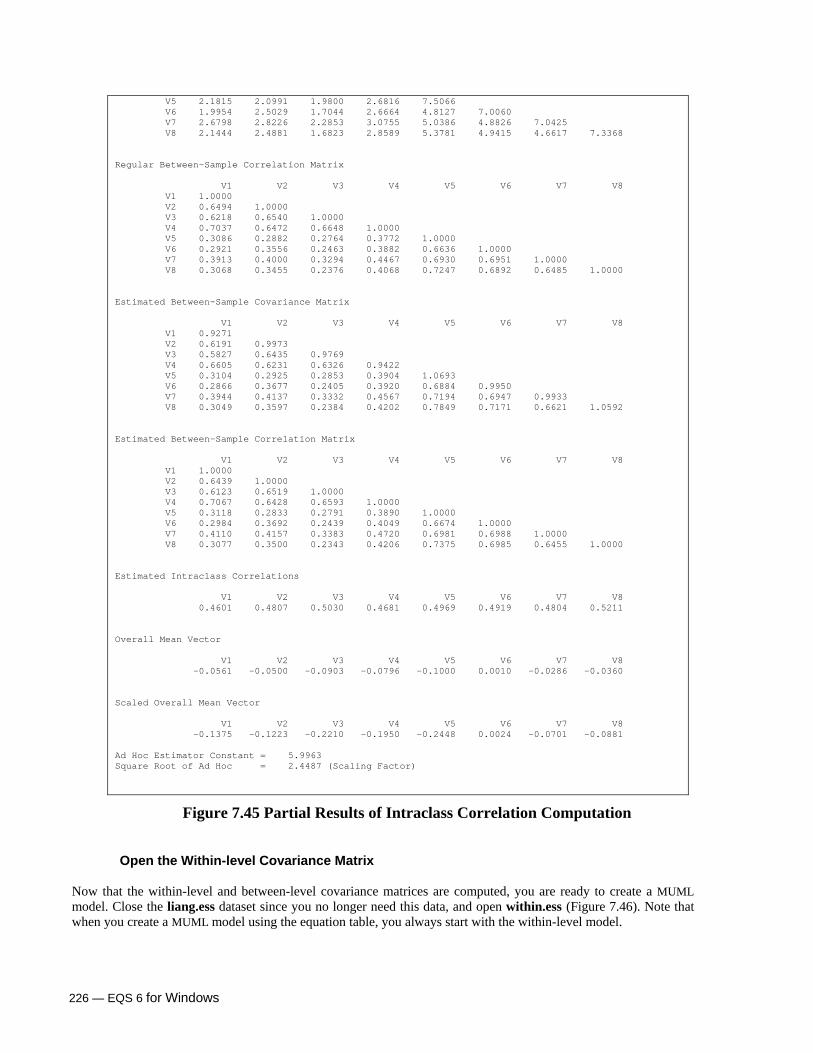
226 — EQS 6 for Windows
V5 2.1815 2.0991 1.9800 2.6816 7.5066 V6 1.9954 2.5029 1.7044 2.6664 4.8127 7.0060 V7 2.6798 2.8226 2.2853 3.0755 5.0386 4.8826 7.0425 V8 2.1444 2.4881 1.6823 2.8589 5.3781 4.9415 4.6617 7.3368 Regular Between-Sample Correlation Matrix V1 V2 V3 V4 V5 V6 V7 V8 V1 1.0000 V2 0.6494 1.0000 V3 0.6218 0.6540 1.0000 V4 0.7037 0.6472 0.6648 1.0000 V5 0.3086 0.2882 0.2764 0.3772 1.0000 V6 0.2921 0.3556 0.2463 0.3882 0.6636 1.0000 V7 0.3913 0.4000 0.3294 0.4467 0.6930 0.6951 1.0000 V8 0.3068 0.3455 0.2376 0.4068 0.7247 0.6892 0.6485 1.0000 Estimated Between-Sample Covariance Matrix V1 V2 V3 V4 V5 V6 V7 V8 V1 0.9271 V2 0.6191 0.9973 V3 0.5827 0.6435 0.9769 V4 0.6605 0.6231 0.6326 0.9422 V5 0.3104 0.2925 0.2853 0.3904 1.0693 V6 0.2866 0.3677 0.2405 0.3920 0.6884 0.9950 V7 0.3944 0.4137 0.3332 0.4567 0.7194 0.6947 0.9933 V8 0.3049 0.3597 0.2384 0.4202 0.7849 0.7171 0.6621 1.0592 Estimated Between-Sample Correlation Matrix V1 V2 V3 V4 V5 V6 V7 V8 V1 1.0000 V2 0.6439 1.0000 V3 0.6123 0.6519 1.0000 V4 0.7067 0.6428 0.6593 1.0000 V5 0.3118 0.2833 0.2791 0.3890 1.0000 V6 0.2984 0.3692 0.2439 0.4049 0.6674 1.0000 V7 0.4110 0.4157 0.3383 0.4720 0.6981 0.6988 1.0000 V8 0.3077 0.3500 0.2343 0.4206 0.7375 0.6985 0.6455 1.0000 Estimated Intraclass Correlations V1 V2 V3 V4 V5 V6 V7 V8 0.4601 0.4807 0.5030 0.4681 0.4969 0.4919 0.4804 0.5211 Overall Mean Vector V1 V2 V3 V4 V5 V6 V7 V8 -0.0561 -0.0500 -0.0903 -0.0796 -0.1000 0.0010 -0.0286 -0.0360 Scaled Overall Mean Vector V1 V2 V3 V4 V5 V6 V7 V8 -0.1375 -0.1223 -0.2210 -0.1950 -0.2448 0.0024 -0.0701 -0.0881 Ad Hoc Estimator Constant = 5.9963 Square Root of Ad Hoc = 2.4487 (Scaling Factor)
Figure 7.45 Partial Results of Intraclass Correlation Computation
Open the Within-level Covariance Matrix Now that the within-level and between-level covariance matrices are computed, you are ready to create a MUML model. Close the liang.ess dataset since you no longer need this data, and open within.ess (Figure 7.46). Note that when you create a MUML model using the equation table, you always start with the within-level model.

EQS 6 for Windows — 227
Figure 7.46 Within-Level Covariance Matrix in within.ess
Build Within-level Model After the data file is opened, click on Title/Specifications from the Build_EQS menu bar. The EQS Model Specifications dialog box appears (Figure 7.39). Again, the information for the data to be analyzed is filled in, as is the default estimation method (ML). Since we are creating a multilevel model in this example, you must click on the Multilevel Analysis option. Once you have clicked on this option, the Additional /SPECIFICATION Options dialog box will appear automatically (Figure 7.48).
Figure 7.47 Specifications Dialog Box for MUML
Figure 7.48 Additional Options
There are four choices in the Multilevel Options group box; check MUML. The edit box labeled Cluster variable is grayed out, because you have had the within- and between-level covariance matrices computed prior to building the model. Click the Continue button in Figure 7.48. EQS will return you to Figure 7.47, which shows (see above) that some information for this multilevel model has been filled in. The model is a two-group model with the structural mean option turned on as well as the multilevel option. You are ready to go to the next step to build equations, variances, and covariances, so click the OK button in Figure 7.47. You will then see a new text window titled within.eqx is opened with some EQS command information is displayed in the window. Since you have seen this window before, we do not show it again.
Build Within-level Equations From the text window titled within.eqx, go again to the Build_EQS menu and select Equations. (We remind you that EQS 6 always uses the data file name as the default EQS model file name. This may help you to associate your model with the data it uses. You can always save the model with a different name before running it.) You will see the Build Equations dialog box (Figure 7.49). This model is a two-factor CFA model with the first four variables loaded on the first factor and the next four variables loaded on the second factor, so enter the number two in the edit box labeled Number of Factors. The MUML model requires a structured mean, and you want to use all the variables in the covariance matrix, so leave Structured Means and Use All Variable options checked. When your dialog box looks like Figure 7.49, click the OK button.

228 — EQS 6 for Windows
Figure 7.49 Build Equations Dialog Box for Multilevel Model The Create Equation dialog box (Figure 7.50) will appear after you have completed the Build Equations dialog box. This dialog box has V1 to V8 and F1 and F2 as row labels. It has V999, F1, F2, and all the V variables as column labels. As we have illustrated before, the rows are used for dependent variables or predicted variables and the columns are used for independent variables or predictors. The model you are building here is a two-factor CFA model with V1 to V4 loaded on F1 and V5 to V8 loaded on F2. Unlike some articles where researchers tend to place the between level first, you must first create the within-level model. The variable means in the within level are always zero, thus, you set the path between measured variables and constant V999 to fixed zero. We assume that you remember how to create these fixed paths by dragging a rectangle to cover all the paths and specifying the start value as zero. Similarly, you can specify the factor loadings of F1 and F2. The complete equation table is shown Figure 7.50.
Figure 7.50 Create Equation for MUML Model
Build Within-level Variances and Covariances Click the OK button when you complete the Create Equation dialog box. The Create Variance/Covariance dialog box appears automatically (Figure 7.51). This dialog box allows you to specify the variances and covariances for the within-level model. You need to click the cell between F1 and F2 because these two factors were correlated when this dataset was created. Click the OK button after you are done with the Variance/Covariance table.
Figure 7.51 Create Variance/Covariance for MUML Model
You have just completed the specifications of the within-level model of the MUML model. The next step is the model for the between level. EQS has made it quite easy to do. After you click the OK button on the Create Variance/Covariance dialog box, the EQS Model Specifications dialog box will appear (Figure 7.52).

EQS 6 for Windows — 229
Build Between-level Model The dialog box is basically a copy of the information from the specification dialog box in the within level. The data file name must be changed to between.ess, which is the data file name in the between-level model. You must click the File Info button on the specification dialog box to get the Input Data Specifications dialog box (Figure 7.53). This dialog box allows you to specify the input data file if it is different from the file shown in the specification dialog box. Click File Name to get the Open File dialog box and select between.ess as the input file. Please note that between.ess should reside within the same folder as within.ess. After between.ess is selected, its file name, number of variables, and number of cases will appear. Please note that the sample sizes on the within level and between level are different. After you correctly select the input file in the Input Data Specifications dialog box, click the Continue button to return to the EQS Model Specifications dialog box, and then click the OK button. That completes the input data for the between-level model. However, be prepared for a shock. The between model required for MUML is not the straightforward between model of the ML method. Rather, the model will include both between and within model parts. This makes MUML much more complex than ML. EQS is designed to hide this complexity from you by facilitating the correct model setup.
Figure 7.52 Between Level Specification
Figure 7.53 Input Data Specifications
As you might expect, you will now see the Build Equations dialog box (Figure 7.54). Unlike the Build Equations dialog box in Figure 7.49, in which the number of factors was left blank for you to fill in, the number of factors here has been filled. You have Number of Variables is 8 and Number of Factors is 12. EQS has calculated the number of factors for you. In fact, EQS has created the between-level model for you based on the model in the within level. You need not do anything else but click the OK button on the Build Equations dialog box.
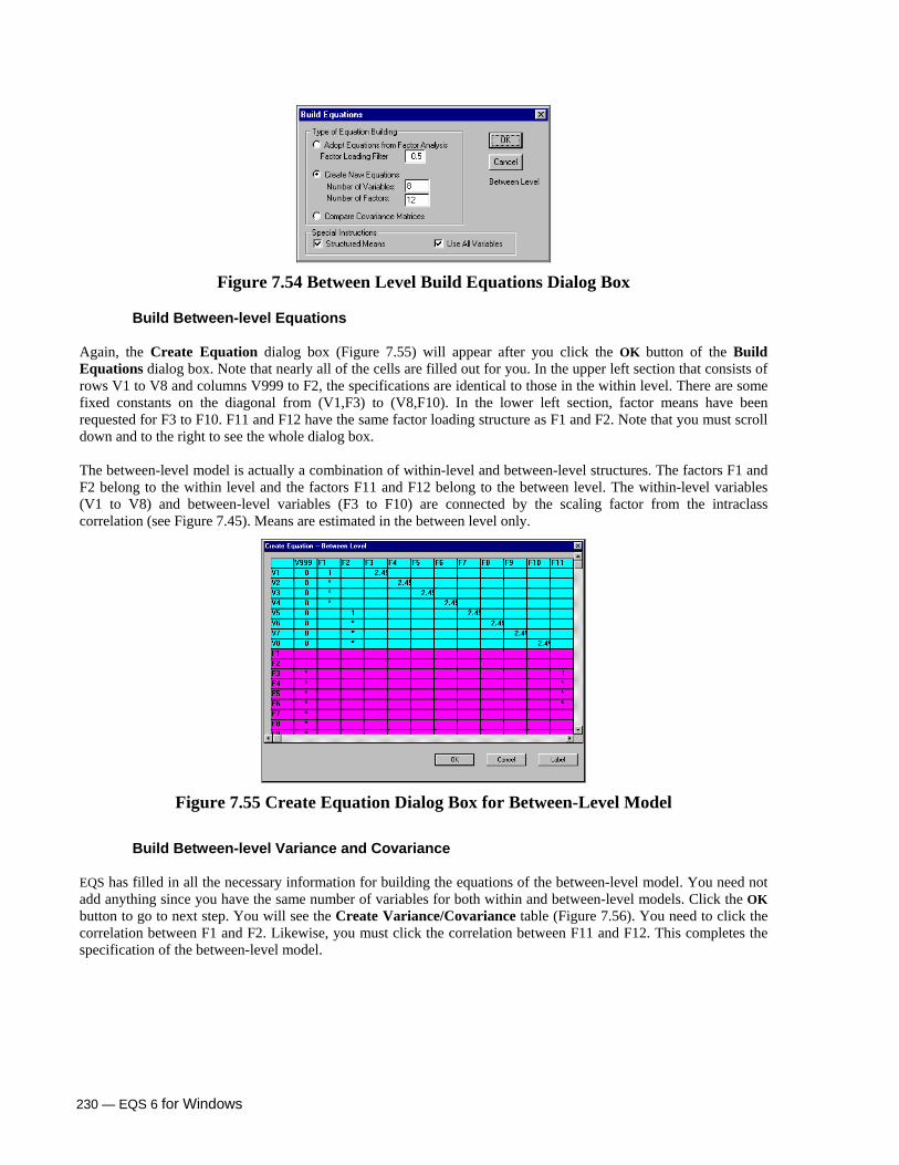
230 — EQS 6 for Windows
Figure 7.54 Between Level Build Equations Dialog Box
Build Between-level Equations Again, the Create Equation dialog box (Figure 7.55) will appear after you click the OK button of the Build Equations dialog box. Note that nearly all of the cells are filled out for you. In the upper left section that consists of rows V1 to V8 and columns V999 to F2, the specifications are identical to those in the within level. There are some fixed constants on the diagonal from (V1,F3) to (V8,F10). In the lower left section, factor means have been requested for F3 to F10. F11 and F12 have the same factor loading structure as F1 and F2. Note that you must scroll down and to the right to see the whole dialog box. The between-level model is actually a combination of within-level and between-level structures. The factors F1 and F2 belong to the within level and the factors F11 and F12 belong to the between level. The within-level variables (V1 to V8) and between-level variables (F3 to F10) are connected by the scaling factor from the intraclass correlation (see Figure 7.45). Means are estimated in the between level only.
Figure 7.55 Create Equation Dialog Box for Between-Level Model
Build Between-level Variance and Covariance EQS has filled in all the necessary information for building the equations of the between-level model. You need not add anything since you have the same number of variables for both within and between-level models. Click the OK button to go to next step. You will see the Create Variance/Covariance table (Figure 7.56). You need to click the correlation between F1 and F2. Likewise, you must click the correlation between F11 and F12. This completes the specification of the between-level model.

EQS 6 for Windows — 231
Figure 7.56 Create Variance/Covariance Dialog Box for Between-Level Model
There is one more important point to consider. The within-level model, acting as a group in a two-group model, duplicates the between-level information, so the two-group model will not be identified. One logical way of avoiding this problem is to constrain the parameters in the within level to be equal to the parameters in the between level. EQS creates the constraint dialog box for you.
Impose Equality Constraints for Within-level Model After you click the OK button on the Create Variance/Covariance dialog box, a Multiple Group Equality Constraints dialog box (Figure 7.57) will appear. This dialog box shows that all free parameters that exist in both groups (levels) have been constrained to be equal across groups. Since the parameters that exist in both groups all belong to the within level, the constraints only affect the parameters in the within level. You need not change anything, just click on the OK button. A complete list of the EQS multilevel MUML model is displayed in Figure 7.58.
Figure 7.57 Equality Constraints for Within-Level and Between-Level Models
/TITLE EQS model created by EQS 6 for Windows --c:\my_eqs_model\examples\within.ess /SPECIFICATIONS DATA='c:\my_eqs_model\examples\within.ess'; VARIABLES=8; CASES=600; GROUPS=2; METHODS=ML; MATRIX=COVARIANCE; ANALYSIS=COVARIANCE; !MULTILEVEL=MUML; /LABELS V1=V1; V2=V2; V3=V3; V4=V4; V5=V5; V6=V6; V7=V7; V8=V8;

232 — EQS 6 for Windows
/EQUATIONS V1 = + 1F1 + 1E1; V2 = + *F1 + 1E2; V3 = + *F1 + 1E3; V4 = + *F1 + 1E4; V5 = + 1F2 + 1E5; V6 = + *F2 + 1E6; V7 = + *F2 + 1E7; V8 = + *F2 + 1E8; /VARIANCES F1 = *; F2 = *; E1 = *; E2 = *; E3 = *; E4 = *; E5 = *; E6 = *; E7 = *; E8 = *; /COVARIANCES F2 , F1 = *; /PRINT FIT=ALL; table-equation; /STANDARD DEVIATION /MEANS /END /TITLE EQS model created by EQS 6 for Windows -- GROUP NUMBER 2 /SPECIFICATIONS DATA='C:\My_EQS_model\Examples\Between.ess'; VARIABLES=8; CASES=120; METHODS=ML; MATRIX=COVARIANCE; ANALYSIS=MOMENT; !MULTILEVEL=MUML; /LABELS V1=V1; V2=V2; V3=V3; V4=V4; V5=V5; V6=V6; V7=V7; V8=V8; /EQUATIONS V1 = + 1F1 + 2.45F3 + 1E1; V2 = + *F1 + 2.45F4 + 1E2; V3 = + *F1 + 2.45F5 + 1E3; V4 = + *F1 + 2.45F6 + 1E4; V5 = + 1F2 + 2.45F7 + 1E5; V6 = + *F2 + 2.45F8 + 1E6; V7 = + *F2 + 2.45F9 + 1E7; V8 = + *F2 + 2.45F10 + 1E8; F3 = *V999 + 1F11 + 1D3; F4 = *V999 + *F11 + 1D4; F5 = *V999 + *F11 + 1D5; F6 = *V999 + *F11 + 1D6; F7 = *V999 + 1F12 + 1D7; F8 = *V999 + *F12 + 1D8; F9 = *V999 + *F12 + 1D9; F10 = *V999 + *F12 + 1D10; /VARIANCES F1 = *; F2 = *; F11 = *; F12 = *; E1 = *; E2 = *; E3 = *; E4 = *; E5 = *; E6 = *; E7 = *; E8 = *; D3 = *; D4 = *; D5 = *; D6 = *; D7 = *; D8 = *; D9 = *; D10 = *; /COVARIANCES F2 , F1 = *; F12 , F11 = *; /PRINT FIT=ALL; table=equation; /CONSTRAINTS (1,F1,F1)=(2,F1,F1); (1,F2,F2)=(2,F2,F2); (1,E1,E1)=(2,E1,E1); (1,E2,E2)=(2,E2,E2); (1,E3,E3)=(2,E3,E3); (1,E4,E4)=(2,E4,E4); (1,E5,E5)=(2,E5,E5); (1,E6,E6)=(2,E6,E6); (1,E7,E7)=(2,E7,E7); (1,E8,E8)=(2,E8,E8); (1,V2,F1)=(2,V2,F1);

EQS 6 for Windows — 233
(1,V3,F1)=(2,V3,F1); (1,V4,F1)=(2,V4,F1); (1,V6,F2)=(2,V6,F2); (1,V7,F2)=(2,V7,F2); (1,V8,F2)=(2,V8,F2); (1,F2,F1)=(2,F2,F1); /STANDARD DEVIATION /MEANS /END
Figure 7.58 Model File for MUML Model
Using /MODEL shortcuts
The previous section illustrated how easy it is to create a MUML type multilevel model using the equation table. But EQS 6 provides another alternative, which is often easier. Let’s consider this EQS command file:
/TITLE EQS Multilevel model using MUML /SPECIFICATIONS data='liang.ess'; case =720; variable=9; method=ml; matrix=raw; analysis=cov; multilevel=muml; cluster=v9; /MODEL (v1 to v4) on f1; (v5 to v8) on f2; cov (f1, f2)=*; /END
Figure 7.59 EQS MUML Multilevel Model with /MODEL
In Figure 7.59, the commands multilevel=muml; cluster=v9; invoke the MUML multilevel method with v9 as the clustering variable. In addition, the model is specified in just a few lines, by using the newly created /MODEL section. Figure 7.42 above, has the exact same commands in the /MODEL section. See the explanation just below Figure 7.42.. The shortcuts provided in the /MODEL section can replace /EQUATION, /VARIANCE, and /COVARIANCE completely with much simpler commands. These shortcuts are especially useful when creating a large model, as a single command can generate dozens of equations. Since the shortcuts are so simple, EQS does not provide any facility to automate their creation. In other words, you have to use a text editor to create an EQS command file (*.eqs) in order to use the /MODEL section. As before, it is assumed that the same model holds for within and between variations, since only a single model can be specified with /MODEL. Of course, once it is expanded, you can modify the model as you like so that its two parts are no longer identical. To run the model as shown in Figure 7.59: while the model is on screen, you pull down the Build_EQS menu and click on Run EQS. EQS will perform the following steps:
1. Create a two-group model. 2. Expand the /MODEL section into a regular EQS model. 3. Create two covariance matrices called within-level and between-level matrices, respectively,
and put them in the EQS model. The within-level matrix goes in the first group and the between-level matrix goes in the second group. Both matrices are inserted in /MATRIX sections.
4. A special structured mean model is set up in the second group, connecting the within- and between-level models, and imposing constraints on the parameters with their counterparts in the first group.

234 — EQS 6 for Windows
5. A constant is inserted to connect the within level and between level. 6. This two-group model will be placed in a temporary file called temp.eqs. 7. EQS will run this temp.eqs and display its results in the output file.
The complete listing of temp.eqs is shown as follows:
/TITLE EQS Multilevel model using MUML /SPECIFICATION VARIABLES = 8; CASES = 600; GROUPS = 2; /LABELS V1=V1; V2=V2; V3=V3; V4=V4; V5=V5; V6=V6; V7=V7; V8=V8; /EQUATIONS V1=1F1+E1; V2=*F1+E2; V3=*F1+E3; V4=*F1+E4; V5=1F2+E5; V6=*F2+E6; V7=*F2+E7; V8=*F2+E8; /VARIANCES /COVARIANCES F2,F1=*; /MATRIX 1.09943 .74293 1.08943 .70047 .68788 .97680 .75072 .72872 .71657 1.08218 .320012 .344958 .269467 .340379 1.09505 .276905 .297802 .262507 .315548 .68489 1.03947 .314829 .341924 .287261 .337245 .72471 .71677 1.08639 .316066 .330952 .252971 .339496 .67168 .64152 .69140 .98574 /STANDARD DEVIATIONS 1.04853 1.04376 .98833 1.04028 1.04645 1.01955 1.04230 .99284 /MEANS 0. 0. 0. 0. 0. 0. 0. 0. /PRINT FIT=ALL; /END /TITLE EQS Multilevel model using MUML /SPECIFICATION VARIABLES = 8; CASES = 120; GROUPS = 2; ANALYSIS = MOMENT; /LABELS V1=V1; V2=V2; V3=V3; V4=V4; V5=V5; V6=V6; V7=V7; V8=V8; /EQUATIONS V1=1F1+E1+2.44873 F3 ; V2=*F1+E2+2.44873 F4 ; V3=*F1+E3+2.44873 F5 ; V4=*F1+E4+2.44873 F6 ; V5=1F2+E5+2.44873 F7 ; V6=*F2+E6+2.44873 F8 ; V7=*F2+E7+2.44873 F9 ; V8=*F2+E8+2.44873 F10 ; F3 = *V999 +1F11+D3; F4 = *V999 +*F11+D4; F5 = *V999 +*F11+D5; F6 = *V999 +*F11+D6; F7 = *V999 +1F12+D7; F8 = *V999 +*F12+D8; F9 = *V999 +*F12+D9; F10 = *V999 +*F12+D10; /VARIANCES

EQS 6 for Windows — 235
/COVARIANCES F2,F1=*; F11- F12= *; /MATRIX 6.65843 4.45530 7.06929 4.19441 4.54628 6.83465 4.71139 4.46508 4.50972 6.73206 2.18153 2.09914 1.98004 2.68159 7.50657 1.99537 2.50285 1.70439 2.66637 4.81271 7.00604 2.67979 2.82260 2.28529 3.07552 5.03859 4.88263 7.04247 2.14444 2.48811 1.68226 2.85889 5.37807 4.94151 4.66169 7.33676 /STANDARD DEVIATIONS 2.58039 2.65881 2.61432 2.59462 2.73981 2.64689 2.65377 2.70865 /MEANS -.056140 -.049962 -.090257 -.079621 -.099984 .000988 -.028607 -.035985 /CONSTRAINTS SET = ALL; /PRINT FIT=ALL; /END
Figure 7.60 Expanded EQS Model Created by /MODEL Note that the sample size in the first group is 600, which is N - K, where N is the total number of observations and K is the number of clusters. The sample size for the second group is K. Also note that /CONSTRAINTS has set all parameters in common across groups (within/between) to be equal, and further, that no entries exist for /VARIANCES. The program adds the free variances automatically.
Build an HLM Multilevel Model We have discussed two different approaches to creating multilevel models in previous sections. Although one method uses maximum likelihood (ML) estimation and other one uses an approximation to obtain the solution, they share the common limitation of handling only two-level models. It is unclear how a model with higher-level data can be handled. For example, a citywide school achievement survey may contain student test scores for each classroom. Each school has contributed different resources on its academic programs; this may affect different classes. City and other government agencies may also allocate unbalanced resources based on the racial composition of the schools. These may all affect student’s test scores. When analyzing such survey data, there are classroom level, school level, and city level data to be dealt with. The complexity of the data may limit researchers who do not have appropriate tools. The last decade has seen the growth of multilevel regression models, often under the name HLM (Hierarchical Linear Model). Such models can handle up to three levels of measured variables. Regression models cannot handle latent variables. EQS has adopted the idea and general approach of HLM and combined it with the ability to handle latent variable models.
The Model Before we go into detail of how to set up an EQS model using the EQS HLM method, let’s review briefly how HLM models are conceptualized. We use a regression model to simplify the example. Assume there is a regression model like the following:
Level 1 (within – unconstrained across clusters): y = a + bX1 + e;
Level 2 (between): a = c + dX2 + e;

236 — EQS 6 for Windows
Unlike ML and MUML approaches, the within cluster parameters are not constrained equal across clusters; there are as many parameter estimates (e.g., “a” and “b”) as there are clusters. These are to be explained at level 2. As you can see, the model in level 2 uses the resulting constant “a” from level 1 as the predicted variable. Because level 2 is a between cluster specification, the sample size in level 2 is always the same as number of clusters in level 1. In other words, HLM will run the model in level 1 separately for each cluster, save the resulting parameter values as data, and pass it on to level 2. The level 2 model uses its own data as well as the data from the level 1 computation.
The Data In the HLM approach, there is one data file for each level, and the organization of the files must match. For example, on a two-level model, if the sample size of level 1 has N observations with c clusters, the sample size for level 2 is c. In the EQS example folder, there are two HLM type multilevel data files. The files are mlevel1.ess and mlevel2.ess. The sample size of mlevel1.ess is 250 observations. The clustering variable for mlevel1.ess is V1, which is the first variable of the data file. This data file has balanced cluster sizes. The sample size for mlevel2.ess is 50 observations, which is the number of clusters in mlevel1.ess. When performing HLM type multilevel model analysis, EQS can handle either balanced or unbalanced data. There is one requirement for the level 1 data file; that all the observations in the same cluster are consecutive cases.
EQS on HLM multilevel model Let’s consider the following EQS model:
/Title Two stage multilevel example (level 1)-- an HLM approach /Specifications data='mlevel1.ess'; var=6; case =250; multilevel=hlm; cluster=v1; analysis=moment; method=ml; matrix=raw; /equations v4 = *v999 + 1f1 + e4; v5 = *v999 + *f1 + e5; v6 = *v999 + *f1 + e6; /variance v999=1; f1 =*; e4 to e6 =*; /end /Title two stage model - (level 2) /Specification data='mlevel2.ess'; var=3; case=50; method=ml; matrix=raw; /DEFINE V4 = (V4,V999); V5 = (V5,V999); V6 = (V6,V999); /equation v4 = *v2 + *v3 + e4; v5 = *v2 + *v3 + e5; v6 = *v2 + *v3 + e6; /variance v2 to v3 =*; e4 to e6 =*; /end
Figure 7.61 HLM Multilevel Model in EQS

EQS 6 for Windows — 237
This EQS model looks just like a regular EQS multilevel ML model except there is a dataset specified in the second group, and a new section labeled /DEFINE. Let’s review these differences in greater detail.
1. HLM Multilevel Method
This model has the format of a two-group model where there are two single group models stacked end to end. The commands “multilevel=HLM; cluster=v1;” says that “this is an HLM multilevel model and V1 is the clustering variable.” It also implies that the data must be a raw data file. The data file mlevel1.ess has six variables with V1 as the clustering variable. There are a total of 50 clusters with 5 observations in each cluster.
2. New /DEFINE Section
A new section labeled /DEFINE is created to define parameter estimates from the previous level as variables in this level. Let’s look back at the model again. There are three statements in the /DEFINE section. The first one is V4=(V4,V999); it means: take the intercepts of V4 in each cluster from level 1 and pass them to level 2 as variable V4. By this token, the V4 on the left hand side of the equal sign and the V4 on the right hand side of the equal sign mean two different things. The V4 variable on level 2 is artificially created from level 1 and is placed there to be used as if it were a real variable. We name the new variable V4 because there are only three variables in mlevel2.ess, which is the data file of the level 2 model. If mlevel2.ess had seven variables, V4=(V4,V999) must be changed to V8=(V4,V999) since V8 is the first available variable in the data file used by the level 2 model. This HLM type of multilevel model is a natural extension of EQS’ multi-sample model. As long as your data are arranged appropriately, the model is quite easy to build. Since this HLM type model is so easy to modify from a standard multi-sample model, EQS does not provide an automatic model-building facility. You must build the model as a *.eqs file. When you have your model ready as shown in Figure 7.61, go to the Build_EQS menu and click Run EQS to run the model. EQS will run the model in level 1 using the data indexed by the cluster variable and continue to run until all clusters are complete for level 1. It will then take the accumulated data from level 1, combine it with the data in level 2 and do another run to complete the model. In our test example, there are two levels. The first level has 50 clusters and the second level has one cluster. Therefore, a total of 51 EQS runs are performed in this multilevel analysis. This version of EQS can handle up to five levels of model if data is available.
3. Estimators and Tests In this illustration we use two dataset namely mlevel1.ess and mlevel2.ess. These two datasets are distributed with EQS 6 for Windows CD. Mlevel1.ess is the data for the first level and has a sample size of 250 with V1 as the clustering variable. As you can see on the data score of V1, each cluster has 5 cases. Mlevel2.ess is the dataset for the second level with sample size of 50. Please note that the sample size of the level 2 equals the number of cluster in level 1. We also have a model called mlevel.eqs (Figure 7.61). Please note that this model and datasets do not produce a nice fitted output. We are using them purely for illustration. The output of mlevel.eqs is shown as follows:
EQS, A STRUCTURAL EQUATION PROGRAM MULTIVARIATE SOFTWARE, INC. COPYRIGHT BY P.M. BENTLER VERSION 6.1 (C) 1985 - 2007. PROGRAM CONTROL INFORMATION 1 /Title 2 Two stage multilevel example (level 1)-- an HLM approach 3 /Specifications 4 data='mlevel1.ess'; var=6; case =250;

238 — EQS 6 for Windows
5 multilevel=hlm; cluster=v1; analysis=moment; 6 method=ml; 7 matrix=raw; 8 /equations 9 v4 = *v999 + 1f1 + e4; 10 v5 = *v999 + *f1 + e5; 11 v6 = *v999 + *f1 + e6; 12 /variance 13 v999=1; 14 f1 =*; 15 e4 to e6 =*; 16 /end 16 RECORDS OF INPUT MODEL FILE WERE READ DATA IS READ FROM mlevel1.ess THERE ARE 6 VARIABLES AND 250 CASES IT IS A RAW DATA ESS FILE TITLE: Two stage multilevel example (level 1)-- an HLM approach *** GROUP 1 OF HIERARCHICAL RUN. VALUE OF CLUSTER VARIABLE IS 1 SAMPLE STATISTICS BASED ON COMPLETE CASES UNIVARIATE STATISTICS --------------------- VARIABLE V4 V5 V6 V999 MEAN 20.8840 9.0960 6.2900 1.0000 SKEWNESS (G1) -.0652 .9901 -.1414 .0000 KURTOSIS (G2) -1.3796 -.3359 -1.7470 .0000 STANDARD DEV. 7.9137 9.5756 6.0520 .0000 TITLE: Two stage multilevel example (level 1)-- an HLM approach MATRIX CONTAINS SPECIAL VARIABLE V999, THE UNIT CONSTANT COVARIANCE MATRIX IS IN UPPER TRIANGLE; MEANS ARE IN BOTTOM ROW OF MATRIX COVARIANCE/MEAN MATRIX TO BE ANALYZED: 3 VARIABLES (SELECTED FROM 6 VARIABLES), BASED ON 5 CASES. V4 V5 V6 V999 V 4 V 5 V 6 V999 V4 V 4 62.627 V5 V 5 39.885 91.692 V6 V 6 23.277 35.648 36.627 V999 V999 20.884 9.096 6.290 1.000
Note: A large portion of output has been edited out. You will see 50 normal EQS outputs stacked end to
end, representing 50 clusters of data each with an EQS run. The summaries of parameter estimates are reported in the following output. The reason that only 45 groups or clusters are reported here is due to the fact that EQS cannot obtain a valid solution for some clusters. In this HLM approach, invalid EQS runs could occur if the sample size in a cluster is insufficient to support a solution. When you have insufficient sample size in a cluster, the portion of the data output where this particular cluster should be placed will be marked as missing data.
SUMMARY STATISTICS OF 45 GROUPS IN HIERARCHICAL RUN PARAMETER ESTIMATES PARAMETER F1,F1 E4,E4 E5,E5 E6,E6 V4,V999 MEAN 67.5629 23.2871 13.0333 8.7010 19.5693 STANDARD DEV. 100.7448 27.5737 20.5884 16.7077 7.8681 SKEWNESS (G1) 3.6227 2.3453 2.4311 3.5115 .4607 KURTOSIS (G2) 14.7439 7.6645 7.0618 12.5854 -.1454

EQS 6 for Windows — 239
LOWER 5% 2.8191 .0000 .0000 .0000 8.1775 UPPER 5% 182.5991 61.1008 43.3906 24.3753 31.9175 PARAMETER V5,V999 V5,F1 V6,V999 V6,F1 MEAN 13.1732 38.9073 7.0308 18.1252 STANDARD DEV. 5.4706 187.5699 5.2821 87.9621 SKEWNESS (G1) 1.3287 5.3256 1.3646 5.4413 KURTOSIS (G2) 2.6927 28.0981 1.8434 29.3899 LOWER 5% 6.3760 .7444 1.2300 -.0033 UPPER 5% 22.7455 4.8476 17.3745 4.5575
Following 50 Univariate Statistics and their summary of all parameter estimates, EQS proceeds to the model in next level. The EQS run in the second level merges data produced (i.e.,parameter estimates) from the previous level and data present in this level for a complete EQS run at the next level. Here this is between level.
EQS, A STRUCTURAL EQUATION PROGRAM MULTIVARIATE SOFTWARE, INC. COPYRIGHT BY P.M. BENTLER VERSION 6.1 (C) 1985 - 2007. PROGRAM CONTROL INFORMATION 17 /Title 18 two stage model - (level 2) 19 /Specification 20 data='mlevel2.ess'; var=3; case=50; 21 method=ml; 22 matrix=raw; 23 /DEFINE 24 V4 = (V4,V999); 25 V5 = (V5,V999); 26 V6 = (V6,V999); 27 /equation 28 v4 = *v2 + *v3 + e4; 29 v5 = *v2 + *v3 + e5; 30 v6 = *v2 + *v3 + e6; 31 /variance 32 v2 to v3 =*; 33 e4 to e6 =*; 34 /end 34 RECORDS OF INPUT MODEL FILE WERE READ DATA IS READ FROM mlevel2.ess THERE ARE 3 VARIABLES AND 50 CASES IT IS A RAW DATA ESS FILE *** WARNING *** THESE CASES ARE SKIPPED BECAUSE A VARIABLE IS MISSING-- 6 16 17 22 27 TITLE: two stage model - (level 2) SAMPLE STATISTICS BASED ON COMPLETE CASES USING ALL DATA, IGNORING CLUSTER INFORMATION UNIVARIATE STATISTICS --------------------- VARIABLE V2 V3 V4 V5 V6 MEAN .5333 .4889 19.5693 13.1732 7.0308 SKEWNESS (G1) -.1336 .0445 .4607 1.3287 1.3646 KURTOSIS (G2) -1.9821 -1.9980 -.1454 2.6927 1.8434 STANDARD DEV. .5045 .5055 7.8681 5.4706 5.2821 TITLE: two stage model - (level 2) COVARIANCE MATRIX TO BE ANALYZED: 5 VARIABLES (SELECTED FROM 13 VARIABLES)

240 — EQS 6 for Windows
BASED ON 45 CASES. V2 V3 V4 V5 V6 V 2 V 3 V 4 V 5 V 6 V2 V 2 .255 V3 V 3 -.017 .256 V4 V 4 -.107 .625 61.907 V5 V 5 -.629 -.286 31.054 29.928 V6 V 6 -.405 .449 33.043 20.079 27.901 GOODNESS OF FIT SUMMARY FOR METHOD = ML INDEPENDENCE MODEL CHI-SQUARE = 93.497 ON 10 DEGREES OF FREEDOM INDEPENDENCE AIC = 73.49733 INDEPENDENCE CAIC = 45.43071 MODEL AIC = 79.21189 MODEL CAIC = 67.98524 CHI-SQUARE = 87.212 BASED ON 4 DEGREES OF FREEDOM PROBABILITY VALUE FOR THE CHI-SQUARE STATISTIC IS .00000 THE NORMAL THEORY RLS CHI-SQUARE FOR THIS ML SOLUTION IS 76.859. ITERATIVE SUMMARY PARAMETER ITERATION ABS CHANGE ALPHA FUNCTION 1 1.356581 1.00000 1.99475 2 .702735 1.00000 1.98209 3 .007235 1.00000 1.98209 4 .000307 1.00000 1.98209
After the iterative summary, the usual EQS output is printed — equations, variances, and covariances, all with optimal parameter estimates for the 2nd-level model.
Continuous and Categorical Correlation Models Typical EQS models are based on analysis of covariances among variables. As you can see, this is the default option under Type of Analysis in Figure 7.73. However, the usual product moment correlations for continuous variables or special correlations for categorical variables also can be analyzed.
Correlation Structures for Continuous Variables You specify that you want to analyze correlations by going to Misc. Options in the specification section, and choosing the option Analysis of Correlation Structure (see Figure 7.73). With the ML option for a normal theory estimator still marked, you will see that Non-normal estimators & corrections (shown at the bottom in Figure 7.63) become available to you. Now you have two options:
1. Check the box marked Robust methods, and at the very bottom you choose the default Test & S.E.. The effect is that EQS sets up the specifications ANALYSIS = CORRELATIONS; and METHOD = ML,ROBUST; in the *.eqx file.
2. Check the box marked AGLS. The effect is that EQS sets up the specifications ANALYSIS = CORRELATIONS; and METHOD = AGLS; in the *.eqx file.
The first option gives our new extension of the Satorra-Bentler robust methodology, including robust standard errors, applied to correlation structures. The second option turns off the ML method and provides an arbitrary

EQS 6 for Windows — 241
distribution alternative. We recommend using the first alternative unless you have a really huge sample, because we would expect the statistics to be trustworthier. Both options use a weight matrix based on a distribution-free approach to correlation structures30 but the AGLS approach requires inverting this matrix. See also Non-normal Estimators and Corrections in this chapter.
Correlation Structures for Categorical Variables You can analyze models with ordered categorical and continuous measured variables. A variable like hair color, taking values of black, brown, or yellow, is not ordered; it is a nominal, not ordinal, variable. It is assumed that ordinal categorical variables are categorized versions of hypothetical underlying variables that are truly continuous and multivariate normally distributed. Unfortunately, these are strong and largely untestable assumptions about unobservables. When the assumptions are true, the correlations between the unknown underlying variables can be estimated by coefficients known as polychoric and polyserial correlations. The correlation between two underlying ordered variables, each of which has been categorized, is a polychoric correlation. The correlation between a continuous variable and the underlying part of an ordinal variable is a polyserial correlation. Structural modeling with such variables proceeds in two major stages:
1. The polyserial/polychoric correlations are estimated without any concern for the structural model under consideration.
2. This correlation matrix is then considered to be a function of more basic parameters, analyzed by methods paralleling those described above for correlations of continuous variables.
In step 1, polychoric and polyserial correlations are computed using the so-called partition maximum likelihood approach of Lee, Poon, and Bentler31. The distribution of these sample correlations was also developed by these authors, who also gave the correct weight matrix to use in step 2, with ANALYSIS = CORRELATIONS;. As above, there are two ways to do step 2. First, you can use the AGLS option. This is the method developed by Lee et. al., who called this a second stage GLS estimation. This is the appropriate method to use in very large samples. However, in small to intermediate sized samples we recommend using the alternative approach we developed for EQS 6. This uses the Robust methods option with Test & S.E. marked (see above). As a result, ML estimation is specified. This gives a good estimator of model parameters. Subsequently, our new versions of the Satorra-Bentler scaling and corrected standard errors are computed, along with many new test statistics.
Implementation We shall use the data file poon.ess that is distributed with the program. This file contains the scores of 200 subjects on eight variables, and will be modeled by a two-factor confirmatory factor analysis model. Open this file now. Then, select the Build_EQS option from the main menu. Give the job an appropriate title. Then, when you get to specifications, you will see the options shown in Figure 7.62.
30 Steiger, J. H., & Hakstian, A. R. (1982). The asymptotic distribution of elements of a correlation matrix: Theory and application. British Journal of Mathematical & Statistical Psychology, 35, 208-215. 31 Lee, S. –Y., Poon, W. –Y., & Bentler, P. M. (1995). A two-stage estimation of structural equation models with continuous and polytomous variables. British Journal of Mathematical and Statistical Psychology, 48, 339-358.

242 — EQS 6 for Windows
Figure 7.62 Model Specification for Categorical Variables
The robust option, ML (by default) is run first, before the statistics are corrected. Note the section titled Categorical Variables. In this section, you must select the categorical variables. Click on the Categorical Variables button in the Advanced Options group box of the Specifications dialog box. You will see the Categorical Variable Specifications dialog box (Figure 7.63) appear.
Figure 7.63 Categorical Variable Specifications Dialog Box Select V7 and V8, and move them to the list box on the right. Click OK. From the Non-normal estimators & corrections, select either the AGLS or Robust methods option. Choose Robust methods, and accept the default choice of Test & S. E.. Then, set up a two-factor model as usual. Variables 1-4 are indicators of factor 1, and variables 5-8 are indicators of factor 2. Fix the first loading of each factor, and let the factors correlate. When you are done, you will see the model file:
/TITLE EQS model created by EQS 6 for Windows -- c:\eqs6\examples\poon.ess /SPECIFICATIONS DATA='c:\eqs61\examples\poon.ess'; VARIABLES=8; CASES=200; GROUPS=1; METHODS=ML,ROBUST; CATEGORY=V7,V8; MATRIX=RAW; ANALYSIS=CORRELATION; /LABELS V1=V1; V2=V2; V3=V3; V4=V4; V5=V5; V6=V6; V7=V7; V8=V8; /EQUATIONS V1 = + 1F1 + 1E1; V2 = + *F1 + 1E2; V3 = + *F1 + 1E3; V4 = + *F1 + 1E4; V5 = + 1F2 + 1E5;

EQS 6 for Windows — 243
V6 = + *F2 + 1E6; V7 = + *F2 + 1E7; V8 = + *F2 + 1E8; /VARIANCES F1 = *; F2 = *; E1 = *; E2 = *; E3 = *; E4 = *; E5 = *; E6 = *; E7 = *; E8 = *; /COVARIANCES F2 , F1 = *; /PRINT FIT=ALL; TABLE=EQUATION; /END
Notice that there are only a few atypical items in this setup, all in the /SPECIFICATIONS section. CATEGORY = V7,V8; identifies these variables as categorical. METHODS = ML, ROBUST; tells the program to do ML estimation followed by robust corrections. ANALYSIS = CORRELATION; tells the program to analyze the correlation matrix. The remaining sections are of the usual form. Go ahead and run EQS now by selecting Run EQS from the Build_EQS menu. Use whatever names you want for the files, and then fetch the output and look at it.
Note: There is one limitation to the current implementation. Consistent with the statistical theory, all measured variables in models with categorical variables must be dependent variables. However, we can trick the theory. If you want to use a measured variable as an independent variable, you can create a dummy factor to represent it. For example, if you want to include V7 in your model as an independent variable, create an equation like V7=F7; and use F7 in the model as if it were V7. Research will be needed to evaluate this procedure.
Output By and large, the usual ME=ML, ROBUST; output is given when used with categorical variables. The normal theory ML method yields the estimates, and then corrections to the chi-square and standard errors are added to the ML output. However, there are some other sections of output in addition. These come immediately after the model file listing:
YOUR MODEL HAS SPECIFIED CATEGORICAL VARIABLES TOTAL NUMBER OF VARIABLES ARE 8 NUMBER OF CONTINUOUS VARIABLES ARE 6 NUMBER OF DISCRETE VARIABLES ARE 2 INFORMATION ON DISCRETE VARIABLES V7 WITH 3 CATEGORIES V8 WITH 3 CATEGORIES
The program has figured out how many categories your variables have. EQS can do this whether or not you declared these variables as categorical in the Data and Information sections. The category information is used in the computations. Information on the polyserial correlations is presented first, for each of the variables in turn. The estimated thresholds are given first, followed by the covariance and correlation estimates. Standard error estimates also are provided:

244 — EQS 6 for Windows
RESULTS OF POLYSERIAL PARTITION USING V 7 -- 3 CATEGORIES THRESHOLDS ESTIMATES STD. ERR -.5112 .0741 .4318 .0767 ESTIMATES VARIABLE COVARIANCE STD. ERR CORRELATION STD. ERR V 1 .4154 .0520 .4154 .0520 V 2 .4442 .0507 .4442 .0507 V 3 .4957 .0493 .4957 .0493 V 4 .4281 .0516 .4281 .0516 V 5 .6181 .0449 .6181 .0449 V 6 .6358 .0427 .6358 .0427 RESULTS OF POLYSERIAL PARTITION USING V 8 -- 3 CATEGORIES THRESHOLDS ESTIMATES STD. ERR -.4566 .0747 .4986 .0779 ESTIMATES VARIABLE COVARIANCE STD. ERR CORRELATION STD. ERR V 1 .3812 .0532 .3812 .0532 V 2 .2654 .0552 .2654 .0552 V 3 .3558 .0539 .3558 .0539 V 4 .4390 .0504 .4390 .0504 V 5 .6220 .0430 .6220 .0430 V 6 .6728 .0396 .6728 .0396
Information on polychoric correlations is presented next. Again, thresholds are computed and then the polychoric correlation estimates are given.
RESULTS OF POLYCHORIC PARTITION AVERAGE THRESHOLDS V 7 -.5044 .4327 V 8 -.4580 .4854 POLYCHORIC CORRELATION MATRIX BETWEEN DISCRETE VARIABLES V 7 V 8 V 7 1.000 V 8 .583 1.000
The above correlations are assembled into the matrix to be analyzed, and typical output follows. With ME=ML, ROBUST; the goodness of fit summary has two sections. The first is for ME=ML. While the ML chi-square cannot be trusted, there are several meaningful new residual based statistics. These include the Browne and Yuan-Bentler-Browne residual-based chi-square tests, and the Yuan-Bentler residual-based F statistic. Then, for ME=ROBUST; the Satorra-Bentler chi-square is given. Among these options, the F test or the Satorra-Bentler tests are most trustworthy. See below32 33 for more information. The Browne test should not be used unless sample size is very large. Of course, with large samples, ME=AGLS; is also a good option, and the output would be modified correspondingly.
32 Yuan, K. –H., & Bentler, P. M. (1998). Normal theory based test statistics in structural equation modeling. British Journal of Mathematical and Statistical Psychology, 51, 289-309. 33 Bentler, P. M., & Yuan, K. –H. (1999). Structural equation modeling with small samples: Test statistics. Multivariate Behavioral Research, 34, 181-197.

EQS 6 for Windows — 245
Multiple Group Structural Means Models The Build_EQS procedure contains a feature that helps to set up multiple group models. In Figure 7.9, there was a check box Multisample Analysis. When you check this, you also must indicate the number of groups in the edit box Groups = . When these choices are selected, the /SPECIFICATIONS that are created in your file contain the statement GROUPS=2; (or whatever number you mentioned). Then you continue specifying your model as you did before. When you have completed specifying the equation and variance-covariance information for the first group, you are immediately taken back to another round of model specifications. That is, you immediately see a title dialog box, then the specifications dialog box, and the equations, and then variances-covariances. The title, of course, should indicate that this is group 2. The specifications should indicate the correct data file or matrix for this group, and the correct number of subjects. The equations and variances and covariances are, by default, duplicates of the ones you provided for the first group. Thus, for all practical purposes, if you have a highly restricted model that is very similar across groups, it is automatically set up for you. In the model file for the last group, when you set up Constraints, you will find that you are prompted automatically for information about the Parameter List and Group List from which you must specify your cross-group constraints. The instructions are self-explanatory, and they follow the previous procedures. The result is that you can specify the cross-group constraints that are the heart of multiple group models. Figure 7.64 shows an example of the Constraints dialog box. If you want the variance (F1,F1), for example, to be equal in all groups, select it. In Group List, ALL GROUPS will become active. Then push the right arrow to create the Constraint Equation, and click OK.
Figure 7.64 Build Multiple Group Constraints Dialog Box with Selection
To run EQS, call EQS as usual.
Reliability Based on a Factor Model
A composite variable is a sum of other variables, for example, V4 = V1+V2+V3. Composites such as V4 are well known, for example, as the total score on a test made up of parts V1, V2, and V3. Another name for a composite score is a scale score, where, in testing or survey research, the scale score may be the sum of the item scores comprising it. Internal consistency reliability coefficients are meant to describe the quality of a composite or scale in terms of its hypothetical common and unique constituents. EQS 6 provides several such internal consistency coefficients automatically, depending on the model setup. See the EQS Manual. The most well-known of these is Cronbach’s alpha. However, the reliability of a composite estimated under the assumption of a 1-factor model

246 — EQS 6 for Windows
underlying the parts is a better true indicator of internal consistency than alpha. Raykov34 showed how this 1-factor coefficient could be computed, and EQS has implemented this method in a convenient way. All you need to indicate are the variables whose composite reliability you want to establish We use holza.ess as the data to illustrate Factor Reliability tests. This dataset has 9 variables with 145 observations. It is frequently used as the sample dataset for factor analysis. To build an EQS model for this test, go to Build_EQS and click on Title/Specification to get the Specifications dialog box (Figure 7.6 ).
Figure 7.7 Specification Dialog for Factor Reliability Test
The dialog box already has all the information filled; you need only click the OK button. After clicking the OK button, a new text window will open and some basic EQS model information will be displayed. Computation of reliability is a special case of an EQS model. Instead of using Equation from the Build_EQS menu, click on Reliability. You will see the EQS Reliability Tests dialog box Figure 7.8).
Figure 7.9 Variable Selection and Factor Structure for Factor Reliability Test
You must select the variables you want to test. In this illustration, choose variables V1 to V4 as a one-factor factor analytic model. The diagram of the factor structure is displayed on the right hand side of Figure 7.10. After completing the variable selection, click the OK button on the EQS Reliability Tests dialog. You will see a complete EQS Reliability model (Figure 7.67) displayed in the text window. Note that there is a new section called “/RELIABILITY” in the model. That section lists the variables that make up the scale total score. EQS will replace this section by EQUATION, VARIANCE, and COVARIANCE sections before the model is run.
34 Raykov, T. (1997). Estimation of composite reliability for congeneric measures. Applied Psychological Measurement, 21, 173-184.

EQS 6 for Windows — 247
Note: You can only perform one reliability test in a single EQS model.
/TITLE EQS model created by EQS 6 for Windows /SPECIFICATIONS DATA='c:\eqs61\examples\holza.ess'; VARIABLES=9; CASES=145; GROUPS=1; METHODS=ML; MATRIX=RAW; ANALYSIS=COVARIANCE; /LABELS V1=V1; V2=V2; V3=V3; V4=V4; V5=V5; V6=V6; V7=V7; V8=V8; V9=V9; /RELIABILITY SCALE=V1,V2,V3,V4; /PRINT FIT=ALL; TABLE=EQUATION; /END
Figure 7.67 EQS Model for Factor Reliability Test After running the one factor model, the program provides the usual program output. After the model chi-square test, you will get a section titles FIT INDICES, and then the section titles RELIABILITY COEFFICIENTS. Among the many coefficients, you will find Cronbach’s alpha, and, in particular, the RELIABILITY COEFFICIENT RHO which is the 1-factor based index. In this example, α=.555 and ρ=.616.
EQS Commands From the beginning of this chapter until now, we have illustrated many sample models. You have encountered the most essential functions in building EQS models. Many more have not been introduced. From here on, we will try to introduce to you all the functions in EQS. Please use this section as reference guide for the capabilities available in EQS.
Title/Specifications Usually, you start building a model by opening a data file. In several examples below, we use manul7a.ess. Then click on Title/Specifications. The dialog box below will then appear.

248 — EQS 6 for Windows
Figure 7.11 EQS Model Specifications Dialog Box from Build_EQS
The model specifications dialog box has the most commonly used options as defaults. This entire box will often be acceptable as is, and typically you can just click OK and proceed. However, you should look at it, to see that it provides the correct options. The dialog box is partitioned as follows:
Title When the dialog box appears, the EQS Model Title edit box is initially filled with “created by EQS 6 for Windows” followed by the data file name. The default title is designed with a purpose. It tells you that the model is generated by EQS 6 and this model is based on manul7a.ess. In case you need to revisit the model months or even years later, you still can identify the source of the model.
Input Data File Information The Input Data File Information field displays the data file name used in the model as well as the number of variables and number of cases. There is also a button labeled File Info. If you want to change the data file that you are going to use in the model, click on the File Info button. Although it is not recommended, you also can invoke EQS model building when no data file is active. Then you must provide the file name, as well as the number of variables and cases. You must click on the File Info button to activate the File Information dialog box so that you can provide this information. If you use an EQS system (*.ess) file, the number of variables, number of cases, type of data, and variables names will be retrieved automatically.
Type of Analysis
Multisample Analysis This methodology is used to create to a model or set of models for more than one group of subjects. This is the appropriate procedure for comparing various parameters across two or more samples. We shall explain more about this option below. Simply stated, the sequence of model specification steps that you make for one group will, with this option, be repeated for each of the other groups. To choose this option, click on the check box, and then specify the number of groups. In EQS 6, you may use up to 100 groups.
Structural Mean Analysis

EQS 6 for Windows — 249
This option is for a Means Structure, or Mean and Covariance Structure Analysis. This methodology allows a model to include intercepts and means to be estimated, including variable and factor means. A conventional structural equation model uses the covariance matrix only. A structured mean model also uses sample means to be modeled.
Multilevel Analysis Multilevel analysis deals with models with hierarchical data. EQS 6 can handle three types of multilevel models. First of all, EQS has implemented a methodology using an ML estimator. Second, EQS has an easy way to specify a MUML methodology developed by Muthén. EQS 6 provides an easy way to compute the WITHIN and BETWEEN covariance matrices and subsequently uses these matrices to build a multilevel model. Third, EQS allows an HLM-like multilevel implementation where model parameters are estimated for each cluster, and then all the estimates within the cluster will be collected and passed to the next level to be analyzed.
Normal Theory Estimators You can choose from three normal theory estimators. They are LS, GLS, and ML, respectively. Normal theory maximum likelihood (ML) estimation is the default, but another method may be more appropriate for your data. For example, non-normal data would probably best be handled by ML, ROBUST. Click on one of the normal theory estimators (i.e., ML) and choose Robust methods from the Non-normal Estimators and Corrections group. Consult the EQS manual for an explanation of the options that are available.
Non-normal Estimators and Corrections If your data are not normally distributed (e.g., your Mardia’s normalized multivariate kurtosis is larger than about 3), you should not trust the test statistics and standard errors that come from LS, GLS, or ML methods. EQS provides several alternative methods to handle this situation, which you specify in the bottom section of Figure 7.12. For technical references, see the EQS 6 Structural Equations Program Manual.
Elliptical If your variables have little or no skew, that is, are symmetrically distributed, with the same degree of departure from normality for all variables, elliptical (E) methods are a good choice because only one extra parameter (the kurtosis parameter) is needed as compared to normal theory methods. Your data’s univariate kurtoses should be homogeneous. However, if the kurtoses differ among the variables, you should use another method. Normal theory methods are special cases of this methodology, i.e., if your data are normal, the E results will be close to the usual normal theory results.
Heterogeneous Kurtosis If your variables are symmetric in distribution, but different variables have different kurtoses, you should consider using the HK method. Although this method was developed over a decade ago, it has not been studied further. It uses the marginal kurtoses of the various variables during estimation. If you check this option, the choices Average versus Geometric Mean become available to you. The Average approach averages the two kurtoses of a pair of variables in weights used for estimating the distribution of covariances, (based on work by Kano, Berkane, & Bentler, 1990)35. The Geometric Mean method takes the square root of their product instead (as developed by Bentler, Berkane, & Kano, 1991)36. The Geometric Mean approach holds for a wider variety of nonnormal distributions, and
35 Kano, Y., Berkane, M., & Bentler, P. M. (1990). Covariance structure analysis with heterogeneous kurtosis parameters. Biometrika, 77, 575-585. 36 Bentler, P. M., Berkane, M., & Kano, Y. (1991). Covariance structure analysis under a simple kurtosis model. In E. M. Keramidas (Ed.), Computing Science and Statistics (pp. 463-465). Fairfax Station, VA: Interface Foundation of North America.

250 — EQS 6 for Windows
should perform better, though there is no empirical data on this. Normal and elliptical methods are special cases of this HK methodology. The real advantage of this method over AGLS and Robust methods is that it can handle models with as many variables as can be handled with normal theory methods.
AGLS The Arbitrary Distribution Generalized Least Squares method is a GLS method that makes no distributional assumptions, that is, variables can have arbitrary distributions. It is often known as the “ADF”, or Asymptotically Distribution Free, method because its distribution free properties are fully justified only in large samples. And indeed, empirical studies show that the AGLS method tends to break down catastrophically in small samples, especially with a lot of variables. In addition to providing the AGLS chi-square, EQS 6 provides two substantially better tests. One is the Yuan-Bentler (1997) corrected AGLS statistic, and the other is the Yuan-Bentler (1999) AGLS F-test. Both of these largely mitigate the problems with the χ2 statistic, with the F-test perhaps being the most reliable. EQS also provides corrected AGLS standard errors based on another paper by Yuan and Bentler. See the EQS 6 Structural Equations Program Manual for details. While the AGLS method is the best choice for truly large samples, better choices are available for not too large samples. Also, this method is hard or impossible to compute if the number of variables is too large (perhaps 30 or more variables), especially with smaller sample sizes.
Robust Methods When you choose this option, two alternative choices become available to you. First, there are the Test & S.E. Corrections. Second, the Case Weights procedure. Technical details and references are given in the EQS 6 Structural Equations Program Manual, but, roughly speaking, the following is what you get:
Test & S. E. Corrections Test & S. E. corrections accept the estimates obtained from a normal theory (elliptical, HK) method such as ML but correct the χ2 statistic and standard errors so that they are more trustworthy. The parameter estimates from these methods can be very good, even under violation of assumptions, but parameter and model evaluating statistics are not trustworthy. Hence, EQS 6 provides several improved test statistics, most of which are in a public program for the first time. These include:
1. Satorra-Bentler scaled χ2. The ML test is scaled (multiplied) by a constant in accord with methods developed by Satorra and Bentler (1994)37. Technically, this corrects the mean of the distribution of test values, but in fact it performs best at the tail where model acceptance/rejection is done. This statistic is the most widely studied and generally accepted best alternative test statistic for model evaluation under nonnormality. It may fail when a model is based on a large number of variables and a very small sample.
2. Browne residual-based statistic. Browne’s (1984)38 test is based on the residual between estimated model and sample covariances, and performs well in huge samples but breaks down in intermediate to small samples. Its advantage is that it is asymptotically (large sample) χ2 distributed.
3. Yuan-Bentler-Browne residual-based statistic. This test is a modification of the Browne statistic proposed by Yuan and Bentler (1998)39 that performs well in intermediate to small samples, while retaining the same large sample optimality as the Browne test. There is some evidence that this test might over accept models at the smallest sample sizes.
37 Satorra, A., & Bentler, P. M. (1994). Corrections to test statistics and standard errors in covariance structure analysis. In A. von Eye & C. C. Clogg (Eds.), Latent Variables Analysis: Applications for Developmental Research (pp. 399-419). Thousand Oaks, CA: Sage. 38 Browne, M. W. (1984). Asymptotically distribution-free methods for the analysis of co-variance structures. British Journal of Mathematical and Statistical Psychology, 37, 62-83. 39 Yuan, K. –H., & Bentler, P. M. (1998). Normal theory based test statistics in structural equation modeling. British Journal of Mathematical and Statistical Psychology, 51, 289-309.
EQS 6 for Windows — 251
4. Yuan-Bentler residual-based F statistic. Also developed by Yuan and Bentler (1998), recent research indicates that this is probably the best test for a wide range of conditions of sample sizes and types of nonnormality.
In addition to correcting the model test statistic, with this option standard errors that are robust to nonnormality are automatically computed. The usual normal theory (e.g., ML information matrix based) standard errors are misleading, typically too small, when variables have heavier tails as compared to the normal distribution. The more accurate robust formula has been in the literature for a long time, e.g., Bentler and Dijkstra (1985)40, and in EQS since 1989. These robust standard errors are printed below the normal theory ones.
Case Weights All of the above methods accept the usual sample means and covariances as data to be modeled. However, when there are outliers or influential cases in a data file, these sample statistics can depend too heavily on those cases. For example, correlations can change substantially by keeping such a case in, or out, of the analysis. The case-weighting methodology from Campbell41 iteratively assigns each observation in a sample a weight in the interval 0-1. Then weighted means and covariances are computed. Outliers are given very small to zero weights, so that they have almost no or no impact on the resulting robust means and covariances to be modeled. If there are no outliers, as in a multivariate normal sample, each case is given a weight of 1.0. Yuan and Bentler (1998)42 extended Campbell’s method to covariance structure analysis, and this is what you find in EQS 6. You can control two constants used in the Campbell procedure, but the defaults work well. In essence, the case-weighting methodology does normal theory ML computations on the Campbell means and covariances, keeps the estimates, and then corrects the test statistics and standard errors so that they are appropriate (since the uncorrected ML ones are not). This means that you get the variety of statistics described above in Test & S. E. Corrections. This is actually a larger set than developed in the Yuan-Bentler paper.
Advanced Options There are four buttons in the Advanced Options group. They are Categorical variables, Missing data handling, Misc. Options, and Delete cases. We will explain the details later when appropriate examples are provided. Let’s only briefly mention what each of these options does.
Categorical Variables This option allows you to specify categorical variables in the model. Unlike the previous version of EQS that only allows 20 categorical variables, EQS 6 allows you to specify up to 200 categorical variables, the maximum number of measured variables permitted in a model. You must select the categorical variables in the variable list on the left, and use the right arrow button to move them to the box on the right. The dialog box below would cause EQS to add the line in boldface to the model:
40 Bentler, P. M., & Dijkstra, T. (1985). Efficient estimation via linearization in structural models. In P. R. Krishnaiah (Ed.), Multivariate Analysis VI (pp. 9-42). Amsterdam: North-Holland. 41 Campbell, N. A. (1980). Robust procedures in multivariate analysis I: Robust covariance estimation. Applied Statistics, 29, 231-237. 42 Yuan, K. –H., & Bentler, P. M. (1998). Structural equation modeling with robust covariances. In A. Raftery (Ed.), Sociological Methology (pp. 363-396). Malden, MA: Blackwell.

252 — EQS 6 for Windows
/SPECIFICATIONS DATA='c:\eqs61\examples\poon.ess'; VARIABLES=8; CASES=200; GROUPS=1; METHODS=ML,ROBUST; CATEGORY=V7,V8; MATRIX=RAW; ANALYSIS=CORRELATION;
Figure 7.13 Categorical Variable Specifications Dialog Box and Partial Model File Once you have specified which variables are categorical, everything else is automatic. All other modeling steps remain the typical ones. EQS knows to compute polyserial and polychoric corelations instead of product moment correlations for the selected variables. You should, however, modify the default ML method by choosing Robust methods and Test & S.E. options. See Correlation Structures for Categorical Variables.
Missing Data Analysis EQS provides several choices in missing data handling. If you have only very few missing scores, you could choose the option Use Complete Cases which does list-wise deletion. However, a generally better option is to choose Use Maximum Likelihood Estimators, which does not delete any cases and uses all data optimally using a so-called EM algorithm to obtain the ML estimates. With this method, you have the option to compute standard errors in two different ways. The default uses the Fisher Information matrix that is typically used with maximum likelihood. The alternative is to use the Observed Information matrix, which involves second order derivatives and may possibly be better in small samples. If you choose the default, you have the dialog box below, which would cause EQS to add the line shown in boldface to the model that specifies the chosen options:
/SPECIFICATIONS DATA='c:\eqs61\examples\amos17.ess'; VARIABLES=6; CASES=73; GROUPS=1; METHODS=ML; MISSING=ML; SE=FISHER; MATRIX=RAW; ANALYSIS=COVARIANCE;
Figure 7.14 Missing Data Handling Dialog Box and Partial Model File However, if your data are not normally distributed, you should also add the robust option that keeps the ML estimates but corrects the chi-square and standard errors for nonnormality, somewhat akin to the Satorra-Bentler corrections. You do this by choosing the Robust methods option, focusing on the Test & S.E. in the /SPECIFICATIONS section. The effect is to add METHOD=ML, ROBUST; to the model specification, thus providing correct statistics based on Yuan and Bentler’s (2000) Sociological Methodology article. A final method you can use with missing data is the choice to Use Pairwise Covariance Matrix. This adds MISSING=PAIR; to the specification. This method for the first time provides correct statistics for correlations

EQS 6 for Windows — 253
computed based on all available cases that have scores on pairs of variables, i.e., no cases are eliminated and no score imputation is done. By default, the Robust methods option is turned on, and METHOD=ML, ROBUST; is also set. The effect is compute ML estimators and then to correct the statistics for non-normality, as in the Satorra-Bentler approach. If there is no nonnormality, the statistics will be correct as well. This method has not been published and is new in EQS. If the sample size is large enough, an alternative to consider is the AGLS method. This method does distribution-free estimation using the pairwise present covariance matrix, as developed by van Praag, Dijkstra, & Van Velzen43 (1985). The complete data AGLS procedure is a special case. However, it should be remembered that the AGLS method tends to break down in small samples. The van Praag et al. weight matrix is used in the ML, Robust approach.
Delete Cases This option allows you to specify cases to be excluded from the EQS modeling run, without deleting the observations from the dataset. It is one way of handling outliers. The dialog box below would cause EQS to add the line in boldface to the model:
/SPECIFICATIONS DATA='c:\eqs61\examples\manul7.ess'; VARIABLES=6; CASES=50; GROUPS=1; METHODS=ML; MISSING=COMPLETE; MATRIX=RAW; ANALYSIS=COVARIANCE; DEL=50;
Figure 7.15 Delete Cases Dialog Box and Partial Model File
Miscellaneous Options Some miscellaneous options in the specification context are found here.
Type of Output File This option allows you choose what kind of output file you want. EQS provides two options. One is a regular text output file, which is the default. The other is in HTML format. This HTML format is very similar to the documents you see on a World Wide Web page. Basically, it is a hypertext document with important sections of the EQS output file listed at the top. You can jump to a section by clicking on it, without scrolling the EQS output to get where you want. The dialog box below would cause EQS to add the line in boldface to the model:
43 van Praag, B. M. S., Dijkstra, T. K., & Van Velzen, J. 25-36.

254 — EQS 6 for Windows
/SPECIFICATIONS DATA='c:\eqs61\examples\manul7.ess'; VARIABLES=6; CASES=50; GROUPS=1; METHODS=ML; MISSING=COMPLETE; OUT=HTML; MATRIX=RAW; ANALYSIS=COVARIANCE;
Figure 7.16 Additional /SPECIFICATION Options Dialog Box and Partial Model File
Multilevel Options This group box allows you to specify the type of multilevel methodology you are going to use. Once a method is selected, EQS will arrange appropriate information to build the model. The default is a one-level model. See examples of multilevel runs, above.
Type of Analysis This option specifies how input data will be treated before an analysis is done. These are the selections:
1. Analysis of Covariance Structure – The input data matrix will be converted into a covariance matrix and the EQS analysis will be performed based on the covariance structure. This is the default.
2. Analysis of Correlation Structure – This option allows you to perform correlation structure analysis. In other words, the reproduced matrix based on your model will be constrained to be a correlation matrix.
3. Analysis of Covariance Structure using Z Scores – All variables will be transformed into Z scores. EQS will perform the analysis using covariance structure statistics. Since the input matrix is a correlation matrix in this option, its output may not be meaningful. You must provide raw data input to use this option.
Loop Option
This option allows you to run the same analysis on equal-sized subsets of a raw dataset. You specify the number of EQS runs, R, in the Loop box. EQS will do R separate runs, using the first N cases, the next N, etc., where N is the number of cases you specify in the EQS Model Specifications dialog box. You must make sure that the total sample size in the data file is at least R times N.
Specify Case Weight Variable You can weight the cases in your data for computing the covariance matrix, using the weights given by the chosen variable. Data values of the case weight variable should be positive. Cases with a zero, negative, or missing weight will not influence the calculations. You can use the original weights given in your specified variable, or use normalized weights that scale your variable internally in EQS to sum to sample size.
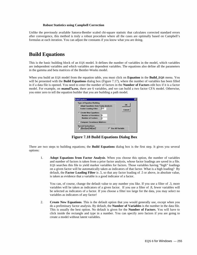
EQS 6 for Windows — 255
Robust Statistics using Campbell Correction Unlike the previously available Satorra-Bentler scaled chi-square statistic that calculates corrected standard errors after convergence, this method is truly a robust procedure where all the cases are optimally based on Campbell’s formulas at each iteration. You can adjust the constants if you know what you are doing.
Build Equations
This is the basic building block of an EQS model. It defines the number of variables in the model, which variables are independent variables and which variables are dependent variables. The equations also define all the parameters in the gamma and beta matrices of the Bentler-Weeks model.
When you build an EQS model from the equation table, you must click on Equation in the Build_EQS menu. You will be presented with the Build Equations dialog box (Figure 7.17), where the number of variables has been filled in if a data file is opened. You need to enter the number of factors in the Number of Factors edit box if it is a factor model. For example, on manul7a.ess, there are 6 variables, and we can build a two factor CFA model. Otherwise, you enter zero to tell the equation builder that you are building a path model.
Figure 7.18 Build Equations Dialog Box
There are two steps to building equations; the Build Equations dialog box is the first step. It gives you several options:
1. Adopt Equations from Factor Analysis. When you choose this option, the number of variables and number of factors is taken from a prior factor analysis, whose factor loadings are saved in a file. EQS searches this file to yield marker variables for factors. Those variables having “high” loadings on a given factor will be automatically taken as indicators of that factor. What is a high loading? By default, the Factor Loading Filter is .5, so that any factor loading of .5 or above, in absolute value, is taken as evidence that a variable is a good indicator of a factor.
You can, of course, change the default value to any number you like. If you use a filter of .3, more
variables will be taken as indicators of a given factor. If you use a filter of .8, fewer variables will be selected as indicators of a factor. If you choose a filter too large for the data, you may select no variables as indicators of any factor!
2. Create New Equations. This is the default option that you would generally use, except when you
do a preliminary factor analysis. By default, the Number of Variables is the number in the data file. This is usually the best option. No default is given for the Number of Factors. You will have to click inside the rectangle and type in a number. You can specify zero factors if you are going to create a model without latent variables.

256 — EQS 6 for Windows
You can specify a Number of Variables, such as 4, that is less than the number in the data file. Unless you uncheck the Use All Variables check box, it will be assumed that you want to use the first so many variables in your data file, such as V1 through V4.
3. Compare Covariance Matrices. This option will be used mostly to compare two or more
covariance matrices. When invoking this option, EQS will ask you for the data files you want to use. After all the data files are specified, EQS will create a multi-sample saturated model and constrain all the parameters to be equal. This is a very convenient way to compare a number of covariance matrices to see if they are statistically equivalent.
4. Structured Means. This is a more advanced feature in EQS in which the means of the observed
variables are explained in terms of fewer parameters, such as the means of the factors. When you invoke this option, the constant variable V999 is created for you to use in your model. Consult the EQS manual for more details on models with structured means.
5. Use All Variables. By default, this option is checked. But if you want to use only certain variables
in your model, there are two ways to do it, depending on whether you want some variables completely removed from the model or only removed from equations.
(a) If your model will use all variables, but you do not want to use all of them as dependent
variables, you can keep the default-checked Use All Variables. When you bring up the Create Equation dialog box shown in Figure 7.12, you would simply not put anything in the rows for those variables that are independent variables. They will then appear in the variance/covariance section.
(b) If you unselect Use All Variables, you will subsequently be given a dialog box called Select
Variables to Build Equations. This box lists all the variables in your file. You click on the variables that you want to use in your model. The ones that are not selected will appear neither in the equations, nor in the variance/covariance section.
Figure 7.19 Create Equation Dialog Box
After clicking OK in Figure 7.20, the Create Equation dialog box (Figure 7.21) will appear. The columns list the possible predictors of each of the dependent variables. In the standard model setup, only Fs and Vs will be predictor variables. In a factor analysis model, only Fs are predictors of the V variables. Predictor variables may be dependent or independent variables, depending on the model. In a factor analysis, the predictor variables are all independent variables. Some cells of the matrix in Figure 7.22 have an asterisk (*) or a 1, while other cells do not. Each nonzero entry refers to a predictor variable to be used for that dependent variable. The 1 refers to a fixed unit path, while * denotes parameter to be estimated. When you click on a cell in the matrix repeatedly, the * will be shown, and then removed, then shown again. Hence by clicking, you can put an * wherever you want, or remove it at will. In our example, the setup is completed and we could click OK and go on. However, we must describe the situation encountered when Create Equation is completely blank. In that case, you will have to decide which dependent variables depend on which predictor variables, and click accordingly. A good way to proceed is to work by columns

EQS 6 for Windows — 257
or by rows. If you work on one column at a time, you are specifying which variables are influenced by that column variable. In Figure 7.23 variables V1, V2, and V3 are the only variables influenced by F1. If you work on one row at a time, you are specifying all the influences on a particular dependent variable, since each row will create one equation. The first row implies an equation for V1, i.e., V1 = ??. The right side of the equation to be generated will contain only those variables, selected from the columns in which you have placed an asterisk or a 1. In the example, only F1 affects V1. EQS uses Es and Ds as residual variables. They are shown in the last column of the equation table. These residuals will be created automatically when the equations are created for Vs and Fs in (e.g.) the manul7a.eqx file, so they are not listed as predictors in the columns of the matrix. If you intended that Es or Ds will have any role other than as standard residuals, you would have to run manul7a.eqx, creating a model file manul7a.eqs and editing that file.
Click, Drag, and Edit a Cell in Equations and Variances/Covariances There are three general procedures that you can use in the Create Equation and Create Variances/Covariances (see below) dialog boxes. We had already noted one of these: clicking and clicking again on a cell in one of these matrices makes the * visible, and then removes it.
Note: Clicking in a cell with a particular mouse may be a bit delicate and it may seem that there is no
response. It may be necessary to experiment to get the right feel for your hardware. There is a simpler way to insert or change the entries in any rectangular matrix of Create Equation or Create Variances/Covariances. Place your pointer in the cell to the left of and above the matrix you want to modify. Click on the mouse button, and drag the pointer, and its attached outlined rectangle, to the cell below and to the right of the lower right corner of the matrix. Check that the rectangle completely covers the matrix you want to change. Then, release the mouse button. For equations, the Start Value Specifications dialog box will appear (Figure 7.24).
Figure 7.25 Start Value Specifications Dialog Box
The Start Value Specifications dialog box has five options, each representing one type of path. This dialog box only appears when two or more cells are selected, allowing you to change a block of cells conveniently. The default option is Fix one and free others. (Note that the default option can be set permanently through the Edit/Preferences menu.) Suppose you want to erase the three values in the F1 column. Place your pointer within the cell defined by V1 and F1 and click. Drag down to the V3,F1 cell and release. The dialog box as shown in Figure 7.26 will appear. Select the option Remove parameters then click the OK button. The F1 column will become blank. Double-clicking on a cell in these matrices will turn the cell into an editable area. You can change the * to 1 or vice versa or even add some start value such as .245* in the editable cell. After typing in the cell, you must hit a tab key or ENTER to save the changes in the cell.

258 — EQS 6 for Windows
If you select Adopt Equations from Factor Analysis in the Build Equations dialog box (see Figure 7.73), the elements of Create Equation are automatically filled in accordance with the elements of the factor loading matrix (e.g., in factor2.ess) that exceed the specified filter value. So Figure 7.74 can be created automatically and we can just click OK to continue. If the results are not to our liking for any reason, we can edit the matrix further in the ways discussed above, before clicking OK.
Variance/Covariance The variances and covariances of independent variables are specified in the Create Variance/Covariance dialog box, which appears automatically when you complete the Create Equation dialog box. The independent variables now include residual E and D variables associated with V and F variables if these are relevant to the model. Figure 7.27 shows the box Create Variance/Covariance for our example. The independent variables in a factor analysis model are Fs and Es. You must place an asterisk in each position that you want to represent as a free parameter. By default, the diagonal elements of this matrix have * inserted in them, and all other elements are empty. Thus by default, the variances of all independent variables are free parameters, and no covariances are parameters. If this is not what you want, you can use the techniques described above to change the elements of the dialog box. In Figure 7.28, an asterisk was added, making (F1,F2) a free covariance.
Figure 7.29 Create Variance/Covariance Dialog Box
Fixing Variances In order to fix the scale of each factor, you must either fix a factor loading at 1.0, or fix the variance of the factor. In our example, EQS 6 for Windows fixed one loading of each factor at 1. Instead, we could have fixed the variances of the factors by clicking on the F1,F1 and F2,F2 diagonal cells of the matrix. The * will disappear from each cell when you click, and the corresponding variance will be fixed at 1.0. In factor analysis, this is a typical practice. It is not necessary to specify the fixed 1 in the diagonal of the matrix; this is done automatically when there is no *. (Remember that, by default, all variances are free parameters.)
Freeing Covariances Covariances are specified in the lower triangle. Do not modify the upper triangle. Each covariance is fixed at zero unless you click on its corresponding cell. Any covariance could be a free parameter, provided that the model is identified. Click on those covariances that you want to be freely estimated. In the case of a confirmatory factor analysis model, factors are usually allowed to correlate. So, in the example, click on the F2,F1 position. The * will appear, indicating a free parameter. If you wanted some correlated errors, those would be specified here as well.

EQS 6 for Windows — 259
Setting Variances and Covariances By Using Drag The drag method of setting parameters can be used in this example. Place the pointer in the upper left corner, above and to the left of F1,F1. Then drag down past the F2,F2 cell. This reverses the previous situation. Starting from the default condition of the dialog box (asterisks on the diagonal and off-diagonal blank), this creates two fixed variance parameters and one free covariance parameter. Or, it reverses that operation if it was previously done.
Constraints You can create any number of linear equality constraints on free parameters by starting at the Build_EQS menu and clicking on the Constraints option. Click on it now. You will see Figure 7.30.
Figure 7.31 Build Single Group Equality Constraints
Figure 7.32 contains five predefined constraint options, a Parameter List in the lower left corner, and a Constraint Equations list in the lower right corner. The predefined constraint options allow you to add frequently used equations to the Constraint Equations list box by checking the appropriate options. Or, you can uncheck the check boxes to remove equations from the list box. Although you can specify most commonly used constraints by activating the check boxes in the Predefined Constraints group box, there may be times when you need to specify individual constraint equations. In order to use constraints effectively, you must learn the EQS Double Label convention for parameters.
EQS Double Label convention for parameters The Parameter List dialog box shows six free parameters. Additional parameters are hidden in the list box, and can be seen by using the scroll bar. In this convention:
1. Variances are denoted by repeating the variable name, e.g., E1,E1 is the variance of E1. 2. Covariances are denoted by the similar double label name, e.g., F2,F1 means the covariance
between F2 and F1. 3. Regression coefficients in equations are denoted by first listing the dependent variable, and
then its predictor. Thus V1,F1 is the factor loading for V1 on F1.
Parentheses are used around the double-label names, since this is a requirement for writing constraint equations.

260 — EQS 6 for Windows
For illustrative purposes, suppose you want the factor loadings for factor 1 to be equal, and also the factor loadings for factor 2 to be equal. Holding down the <Ctrl> key, find each of the double-label names (V2,F1), and (V3,F1) in turn, and, click on each one to select it. Then, click on the right-arrow key. This creates the first equality constraint. Then, you do the same thing for the factor loadings on factor 2. Finally, click on OK. You will see in manul7a.eqx that the model file now contains the constraints that you selected:
/CONSTRAINTS (V2,F1)=(V3,F1); (V5,F2)=(V6,F2);
Of course, you should have an adequate rationale for selecting such equality constraints. Note that equality constraints of this sort are not scale invariant. If these particular equalities are consistent with the data, they could cause model rejection if we were to rescale some of the variables. To illustrate, if we scale V2 by moving the decimal place on its data values, then its variance, covariances, and factor loading, would change as well. So the loadings (V2,F1) and (V3,F1) would have to become unequal to fit the data.
Note: Equality constraints can be placed only on free parameters, and EQS 6 for Windows does not let you use a fixed parameter. In addition, you should remember that EQS also permits you to set up complicated general linear equality constraints. These are not facilitated with Build_EQS. See the EQS 6 Structural Equations Program Manual for more information.
Inequality Constraints EQS automatically imposes the inequality constraint that variances of free parameters should be nonnegative, and that correlations between two variables with fixed 1.0 variances should lie in the interval ±1. You can override these default inequalities, and impose your own, using the Inequality option of the Build_EQS menu to get the dialog box shown in Figure 7.33.
Figure 7.34 Build Inequality Constraints Dialog Box
The inequality constraints in EQS are boundary constraints, permitting you to set limits for all free parameters. You can specify the constraint by entering the bounds in the edit boxes Lower Range and Upper Range. Then select the parameter(s) you want to constrain, and click the Create button. To specify more than one parameter in the Parameter List, hold down the <Ctrl> key as you click on each one. Only free parameters appear in this list. To delete a constrained equation, select the equation in the bottom list box labeled Constrained Equation List, and click the Delete button.

EQS 6 for Windows — 261
For example, to force the estimated factor correlation to be nonnegative, enter the number zero in the Lower Range, click on (F2,F1), then click on Create and click the OK button to exit. You will see the following lines appear in your model file.
/INEQUALITY 0<(F2,F1);
Lagrange Multiplier Test The LM test, or Lagrange Multiplier test, is a test designed to evaluate the statistical necessity of one or more restrictions on a model. The restrictions that are evaluated are, typically, whether a parameter that has been fixed to a given value is appropriately fixed or might better be left free to be estimated, and whether an equality constraint is appropriate for the data. For a discussion of the LM test, and how to use it in EQS, see Chapter 6 of the EQS 6 Structural Equations Program Manual.
Default Test LM tests are probably the most technically demanding to use in their full generality. That is because an understanding of the Bentler-Weeks matrices is really imperative. If you do not want to study this material in the EQS manual, we suggest that you just use the default LMtest procedure. This is implemented via the LMtest option from the Build_EQS menu. When you click on the LMtest option, you see the dialog box in Figure 7.35.
Figure 7.36 Build LMtest Dialog Box
For the default test, you would just click OK. (However, you should not click OK yet if you want to follow the examples on Test Individual Fixed Parameters and Build BLOCK and LAG.) When you click OK, you will get the following lines in your manul7a.eqx file, which indicate that 11 parameter sub-matrices will be searched for fixed parameters that might better be free.
/LMTEST
PROCESS=SIMULTANEOUS;
SET=PVV,PFF,PDD,GVV,GVF,GFV,GFF,BVV,BVF,BFV,BFF;
If you are new to modeling and EQS, just click OK to accept this default. Otherwise, you may wish to study some of the additional options that we shall mention in turn. We only provide cursory descriptions; see the EQS Manual for detailed information.

262 — EQS 6 for Windows
Process Control for LMtest As you see in the above example, by default ten sub-matrices, or groups of parameters, are searched for possible parameters to add to a model. You may consider some of these groups more important than others, or you may not care. The default option, Simultaneous Process, suggests that you want to find the most important missing parameters, by the LMtest criterion. Simultaneous Process also suggests that you do not particularly care whether these parameters are factor loadings or any other type of parameter. If you click the radio button Sequential Process, parameters are selected from the first group in the SET command. Parameters in the next listed group are only searched when there are no more significant parameters in the first group, and so on. If you select this option, you should be sure that SET lists the parameter groups in order of their importance to you. Choose the option Separate Process when you want to obtain several separate LMtests, one for each group. The results based on one group do not take into account what might happen in another group. This is, of course, unrealistic, since the parameter estimates would correlate if they were freed. But it gives you a view of each part of potential model modification without being affected by other parts.
Test Groups of Fixed Parameters You can select the groups of fixed parameters to test with the check box shown in Figure 7.37. By default, it is not checked. If it is checked, you can select or deselect any of the matrix sections shown in the bottom part of the dialog box. As you can see, the groups on the left are parts of the variance/covariance matrix of independent variables, the P?? options. The ?? refer to part of a particular group. Since the only types of potential independent variables are V, F, E, and D, the various options are PVV, PFV, etc. as shown. For example, PFV includes all covariances between independent F’s and independent V’s.
Note: Correlated errors, which would appear in PEE, are not selected by the default option. So if you are
interested in correlated errors, you must check that box. Regression parameters always involve Dependent variables. The only possible dependent variables are V and F variables, so there are only two rows in each of the sections on the right. The predictor might be an independent variable, in which case it appears in the G?? matrix, or another dependent variable, in which case it appears in the B?? matrix. These two matrices are shown in the right part of the dialog box, under Dependent ← Independent (for G?? groups) and under Dependent ← Dependent (for B?? groups). For example, a factor loading is either in GVF, if the factor is an independent variable, or BVF, if the factor is a dependent variable. (Remember that the first variable listed in the pair is the dependent variable, and the second, the predictor. So GVF represent paths from Fs to Vs.) For consistency with the Bentler-Weeks technical notation, the P, G, and B matrices involved are abbreviations of names of Greek letters. That is, P = Phi, G = Gamma, and B = Beta.
Test Individual Fixed Parameters The LM test has its best statistical rationale if you have an a priori hypothesis in mind. Then you should specify your test by picking the option Test Individual Fixed Parameters. The dialog box shown in Figure 7.38 will appear. As you can see, you must specify the matrix.

EQS 6 for Windows — 263
Figure 7.39 LMtest on Individual Fixed Parameters By default, the PHI matrix is checked. The possible independent variables in your model appear in the list boxes on the bottom left. When you select one variable from each list by clicking on its name, and then click on the right-arrow, a parameter such as (E3,E1) is created in the Parameters to be tested list box shown on the bottom right. For example, to create an a priori test on (E3,E1) and (E4,E2), click E3 in the first column and E1 in the second column and click on the right-arrow key; then repeat with E4 and E2. Then click OK in this dialog box. You get back to Figure 7.79 . Do not click OK here yet, because we want to discuss Build Block and Lag below. However, when you do click OK in Figure 7.79 , you will have an a priori test, which looks as follows:
APRIORI=(E3,E1),(E4,E2);
Obviously, as shown in Figure 7.40, you can also select Parameters in GAMMA Matrix or Parameters in BETA Matrix by clicking on the appropriate radio buttons. By default, as shown above, you get an a priori test. In such a test, the parameters are actually evaluated in a forward stepwise fashion depending on their importance. If you want to have the parameters enter the test in a particular sequence, you should click on the check box Test Parameters in the Order Generated. We really do not want to use an a priori test in this example, so click on Cancel in Figure 7.41 so that you are back to the default test.
Build Block and Lag The LMtest can take up so much computer space that you may not be able to run it unless you are selective about parameters that you want to evaluate for inclusion in the model. The feature shown in the bottom right of Figure 7.79 , Build BLOCK and LAG, permits you great control of the LMtest. Before explaining how to set up these features with Build_EQS, we would like to review their purpose. Variables used in structural modeling can often be ordered implicitly or explicitly along a time dimension. For example, data may be gathered in three annual waves. In such a case, one can make a strong a priori assumption that causal processes that might be specified among the variables should also be ordered in time, i.e., that no “backward in time” causal paths should be permitted. If the waves of measurement occur at T1, T2, and T3, then only paths of the type T1 → T2, T1 → T3, and T2 → T3 would be appropriate. A backward path of the type T3 → T1 would not be appropriate. The BLOCK feature of the LM test is designed to assure that backward paths are eliminated from the LM test. As a result, nonsense paths are avoided, and much larger sets of restrictions can be evaluated at the same time. When there are three periods of measurement, we say that the variables can be grouped into three blocks.

264 — EQS 6 for Windows
We discuss how to use these features with any *.eqs file first. This gives a bit more technical detail than necessary to actually implement the procedure from Build_EQS. How to do that is discussed subsequently. You will see that most of the hard work is actually done by the program.
Technical Background on Block and Lag To implement this feature, three commands must be used at the same time in the /LMTEST section of the program setup: SET, BLOCK, and LAG.
1. SET. This is the standard command of the LM test, illustrated above, that specifies which sub-matrices of parameter matrices are to be investigated by the LM test. In simple applications of the LM test, you can omit the SET command. Then default sub-matrices are chosen. When used with the BLOCK feature, however, no default sub-matrices will be chosen, and those desired for analysis must be stated.
2. BLOCK. The BLOCK command, which permits one to group variables into blocks, partitions the
matrices specified in SET into smaller sub-matrices for analysis and specifies the direction of possible paths. It also specifies possible covariance linkages among variables to be included or eliminated.
Only V and F variables can be listed; the program will search for E and D variables and group them
appropriately, based on their correspondence to V and F variables. BLOCK will group together into a single block all of the V and F variables that are listed together, where the variables can be listed individually or in sequence via TO or dash, e.g. V5-V9.
When listed separately, each variable must be separated from other variables by a comma. Each
block must be surrounded by a pair of parentheses. If there is more than one block, a comma must separate the blocks.
So, for example: BLOCK = (V1-V3,F1), (V4-V6,F2), (V7-V9, F3); creates three blocks of variables
corresponding, for example, to three measurement times. V1-V3 and F1 are in the first block. V4-V6 and F2 are in the second block. V7-V9 and F3 are in the third block. The sequence of the blocks indicates the directional sequence in which paths are permitted. That is, only “forward” paths or covariances will be analyzed. (If you want to shift the direction of the paths, you must reverse the sequence listing of the blocks.) Still greater control is made possible by the LAG command.
3. LAG. The LAG specification defines the “time” lag desired for paths between variables in the LM
test. Possible values are LAG = 0; up to LAG = b-1; here b is the number of blocks created by the block statement.
LAG = 0; means that only variables within the same block will be selected; with 3 blocks, there
would be 3 possible sets of within-block paths or covariances to evaluate. With LAG = 1; only paths or covariances across adjacent blocks would be evaluated. For example, LAG=1; might evaluate from T1 to T2 and from T2 to T3. If you want to study the cross-block effects from T1 to T3, you would write LAG = 2;.
In typical practice, one might consider only LAG = 0; in one analysis, LAG = 1; in another analysis,
and so on. However, you can specify several lags simultaneously, for example, LAG = 1,2,4;. When LAG is not specified, a default of ALL is implemented, i.e., 0,1, up to and including b-1.

EQS 6 for Windows — 265
Examples of the directional blocking feature are as follows:
/LMTEST
BLOCK = (V1,V7,V9,F1), (V2,V3), (F2,V4,V5,V6), (F3,V10 TO V15);
SET = BFF, BVV;
LAG = 0;
In this example, there are four blocks, and only paths within each block will be evaluated. Paths are to be of the type involving regression of dependent Vs on other dependent Vs, and dependent Fs on other dependent Fs.
/LMTEST
BLOCK = (V1 TO V5), (V6 TO V10), (V11 TO V15);
SET = PEE;
LAG = 0;
In this example, correlated errors are evaluated, but only covariances within blocks are to be searched. If LAG = 1; had been used instead, only cross-time covariances between adjacent blocks would be evaluated.
Block and Lag in Build_EQS Fortunately, most of the difficult technical specification is done automatically for you in EQS 6 for Windows, though the concepts are certainly important for you to know. First, in the basic Build LMtest dialog box shown in Figure 7.79 , and discussed above, it was made clear how to select sub-matrices to study. These are selected initially, and determine the SET command as you have seen. Only BLOCK and LAG remain to be specified. When you click on the Build BLOCK and LAG button in the Build LMtest dialog box, you will see Figure 7.42. As you can see, all of the V and F variables are displayed in the Variable List box on the bottom left.
Figure 7.43 Build BLOCK and LAG Dialog Box
Holding down the <Ctrl> key, select V1, V2, V3 and F1 in turn, to define your first block. Then click on the right-arrow key, and they are placed into the BLOCK List, as shown below. Then you select V4, V5, V6 and F2 for the second block and click on the right-arrow key. You can see both blocks in Figure 7.44.

266 — EQS 6 for Windows
Figure 7.45 Build BLOCK and LAG Dialog Box with Blocks
When you are finished defining blocks, click on the LAG button. The LAG list displays 0, 1, and you can select the lag or lags that you want. When you are finished, click on OK. This returns you to the Build LMtest dialog box. When you are satisfied, click OK. In this example, click CANCEL instead, since blocking makes no sense. The variables are not time-ordered. When you get back to the Build LMtest dialog box, click OK to get the LM test lines into manul7a.eqx.
Wald Test The Wald Test is a test on the free parameters. It evaluates whether a free parameter could possibly be zero in the population. When you click on the Wald test option from the Build_EQS menu, the dialog box in Figure 7.46 will appear.
Figure 7.47 Build Wtest Dialog Box
The following are the Options available in the Build Wtest dialog box:

EQS 6 for Windows — 267
PVAL
PVAL is the probability value used in Wtest. It is a multivariate probability value for a parameter to be excluded from the model. For example, if a parameter test has a probability value greater than PVAL, that parameter may be dropped from the model. By default, PVAL for Wtest is set to .05, but you can change this value in the edit box.
Priority of testing
You can specify whether parameters should be tested against a Zero Constant or some other Non-Zero Constant. Zero Constant is the default test. Most parameters are tested if they are significantly different from zero. See RETEST in the Print section, below, for tests on nonzero constants.
Parameters never to be tested
There may be some parameters that we would like to keep in the model. For example, factors and factor correlations are the parameters we are most interested in. They should always be kept in the model. The list box on the left Parameter list uses the double-label naming convention to show all free parameters. Select those parameters that you would not want to drop even if their estimates were not significantly different from zero. When specifying the parameters not to be tested, highlight the parameters on the left and use the right-arrow to move them to the list box on the right, Never-drop list. EQS will create a NOFIX command containing the list of parameters not be tested.
Compare with sub-model
When this option is on, EQS will run one additional model with some parameters dropped from the original model. After printing the output for your model, EQS will drop some parameters, based on the Wald test results, and run the smaller model. The results will include a chi-square test for Wald comparison, with degrees of freedom and tail probability.
Parameters tested to be dropped
If you choose Parameters tested to be dropped, you can select free parameters from the list box labeled Parameter list on the left and move them to the Wtest parameters list box on the right. There are two ways to test the parameters. One way is to test based on the value of parameters’ chi-square and the other is based on the sequence of the parameters in the list. The EQS manual explains that the former is a backward-stepping procedure with no particular order of stepping specified (APRIORI), while the latter specifies the procedure in a given, hierarchical way (HAPRIORI).
If you click OK, the material would be entered into the manul7a.eqx file in the usual way. Instead, press Cancel to eliminate these choices, since we do not plan to use them.
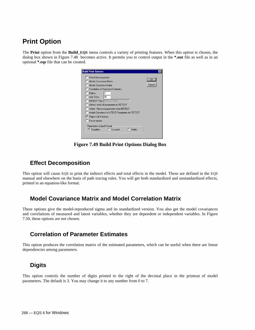
268 — EQS 6 for Windows
Print Option The Print option from the Build_EQS menu controls a variety of printing features. When this option is chosen, the dialog box shown in Figure 7.48 becomes active. It permits you to control output in the *.out file as well as in an optional *.eqs file that can be created.
Figure 7.49 Build Print Options Dialog Box
Effect Decomposition This option will cause EQS to print the indirect effects and total effects in the model. These are defined in the EQS manual and elsewhere on the basis of path tracing rules. You will get both standardized and unstandardized effects, printed in an equation-like format.
Model Covariance Matrix and Model Correlation Matrix
These options give the model-reproduced sigma and its standardized version. You also get the model covariances and correlations of measured and latent variables, whether they are dependent or independent variables. In Figure 7.50, these options are not chosen.
Correlation of Parameter Estimates This option produces the correlation matrix of the estimated parameters, which can be useful when there are linear dependencies among parameters.
Digits This option controls the number of digits printed to the right of the decimal place in the printout of model parameters. The default is 3. You may change it to any number from 0 to 7.
EQS 6 for Windows — 269
Line Size This option determines whether the output file will be in standard 132-column format or narrow 80-column format. The next four options deal with a practical feature, called RETEST, which has been incorporated in recent versions of the EQS program. You must specifically select RETEST if you want it.
RETEST The RETEST option saves a substantial amount of computer time, helping in program convergence of multiple job runs. Also, RETEST makes it easier for you to do a sequence of model modifications. When specified, RETEST takes the final parameter estimates from a completed EQS run and inserts them into a new *.eqs file. Specifically, RETEST creates new /EQUATION, /VARIANCE, and /COVARIANCE sections that contain the optimal parameter estimates from the just-completed run. You can submit that new file, with only minor modifications, for another EQS run. As you see in Figure 7.51, you implement RETEST by checking the list box for RETEST File and typing a file name in the edit box. A default name is provided, but it is always better to use a meaningful name, e.g. the next number in a sequence of models that you plan to run. If the current model file is manul7a1.eqx, an appropriate name might be manul7a2.eqs. Appropriate statements will be added to the *.eqx file, such as: /PRINT
digit=3;
linesize =80;
RETEST=‘manul7a2.eqs’;
lmtest=yes; wtest=yes;
based on the options checked in the dialog box. The new file (manul7a2.eqs in this example) will contain a copy of the input file (manul7a1.eqx), followed by new /EQUATIONS, /VARIANCES, and /COVARIANCES sections, based on final optimal parameter estimates. After you complete the modeling run, and have evaluated your *.out file, you can then bring up the new file manul7a2.eqs. You must edit it to delete parts of the file that are obsolete, and to update the model in the desired way. For example, the /TITLE may need to be changed. The /SPECIFICATION section may be perfectly acceptable, or may need to be modified. The old /EQU, /VAR, and /COV sections, at the top of the file, can typically be replaced by the new sections at the bottom. Other sections, such as /LMTEST, may need to be modified to be appropriate to the next run. The RETEST file name must be changed, otherwise the *.eqs file will be overwritten. As usual, the file to be submitted for an EQS run must end with /END.
LMtest - Add LM parameters to RETEST This option takes parameters that are significant in the multivariate LM test and automatically adds them to the /EQUATIONS, /VARIANCES, and /COVARIANCES as needed. You can recognize these newly added parameters in your model setup because they contrast with the original parameters. The parameters from the original run will have optimal estimates, while the parameters from the LM test results will only have * next to them. Of course, you should only accept those new parameters that make sense.
Wtest - Remove parameters from RETEST

270 — EQS 6 for Windows
You can use this option to flag parameters in the new file that were not significant in the previous run, based on the multivariate Wald test. To differentiate between significant and nonsignificant parameters, note that:
4. All significant free parameters will have an * and the optimal estimate in front of the *. 5. Nonsignificant parameters will have the number 0 next to them.
An example might be V1 = 0F1 + .6*F2 + E1; the parameter (V1,F1) will be eliminated from the next run, since the coefficient is fixed at zero. If you decide to keep the parameter as a free parameter, you simply add an * after the zero. You may also replace the zero by a different start value. Wtest suggestions must always be taken with a grain of salt. For example, we would never remove variances as parameters even if they were not significant.
Attach Constants to WTEST Parameters for RETEST This option, when chosen, adds a line in the model file WPARAMETER=YES; the new line generates some commands in the new RETEST file. Specifically, it creates
/WTEST
APRIORI=(E1,E1):4.38,(E2,E2):3.54,...,(V6,F1):0.00;
which specifies a Wald test for fixed parameters. The numbers are optimal values from the previous run. In the next run, after selecting the parameters of interest, the program will do a Wald test that compares final estimated values to the fixed values. When the fixed values are the values from a prior model run, this procedure can evaluate changes in model estimates due to changes in the model specification. For example, the effects of correlated errors can be evaluated this way. Of course, any fixed nonzero values can be tested. You can omit the numerical values 0.00. This means that just writing (V6,F1) would work in the above example. If you want to test zero constraints first, you must add PRIORITY=ZERO; in the /WTEST section above. When testing a Wtest with a set of constraints, you also obtain a rank correlation of the constants and optimal estimates. This can evaluate the stability of estimates due to model changes.
Report Full Fit Indices
Another option shown in Figure 7.52 allows you to request that EQS compute and print a wider range of fit indices along with the standard options. By default, this option is turned on. The manul7a.eqx file will include the lines:
/PRINT FIT=ALL;
The output will include these additional indices: Bentler-Bonett’s Normed and Nonnormed Fit Indexes, Bentler’s Comparative Fit Index, Bollen’s IFI Fit Index, McDonald’s MFI Fit Index, LISREL’s GFI and AGFI Fit Indexes, Root Mean Squared Residual (RMR), Standardized RMR, Steiger’s RMSEA, and 90% confidence interval of RMSEA. You will find the formulas in the EQS Manual. If you do not want these indices, you may uncheck this option.
Factor Means When you have run a covariance structure model, this option will print factor means and the Bentler-Yuan modified test for a potential structured means model.

EQS 6 for Windows — 271
Report Equations in Equation, Compact, or Matrix format By default, the equations, variances, and covariances are printed in Equation format. For details, see the EQS manual. The Matrix option instructs EQS to report the results in matrix format. For each predictor on the right side of an equation, all of its coefficients in the equations are lined up vertically in one column. The variance-covariance matrix of independent variables is printed as the lower triangle of a symmetric matrix, with one row and column for each independent variable. Positions in the matrices that do not correspond to parameters are left blank, so that this option will produce longer output.
The Compact option will cause EQS to print all parameter values in a compact table. For large models, this option will produce much shorter output that the default. The following is an example of the print options:
/PRINT fit=all; table=matrix; scaled=yes; fmeans=gls;
We do not need RETEST right now, so just press Cancel if you have been following along on your computer.
Technical Option The Technical option from the Build_EQS menu controls the convergence process. When you select this option, a dialog box as shown in Figure 7.53 appears.
Note: In order to change a value in an edit box on the right, you must check the appropriate check
box on the left, and type the new value in the edit box.
Figure 7.54 Build Technical Options Dialog Box
Normal Theory Iterations This option specifies the maximum number of iterations EQS will run when normal theory methods are requested. These methods include LS, GLS, and ML. When a model is running, EQS will evaluate the condition of convergence. When the condition is met, EQS will complete the model and prepare the output. If a model does not converge, EQS will continue the iterative process until the maximum number of iterations is reached. Then the model will be terminated and output information will be prepared at that solution. The default number of iteration is 30 and can be changed through the dialog box or through the Edit/Preference menu. In the *.eqx file, this appears as:
/TECHNICAL ITERATION = 40; ! Increase maximum number of iterations to 40

272 — EQS 6 for Windows
An important option to remember is ITERATION=0; The effect is to compute the model based only on the start values you provide.
Elliptical Iterations
In EQS, the elliptical method uses a linearized process in which only one iteration is done unless you specify otherwise. You can specify your maximum number of iterations in the edit box associated with the elliptical method. In the *.eqx file, this appears as:
/TECHNICAL EITERATION = 30; ! Increase elliptical iterations to 30
AGLS Iterations
The AGLS method, like its normal theory counterpart, is iterated until the model converges or the maximum number of iterations is reached. The default number of iterations is 30 unless you specify otherwise in the edit box associated with AGLS (ADF) Iterations. In the *.eqx file, this appears as:
/TECHNICAL AITERATION = 40;
Convergence Criterion
The convergence criterion, based on changes in parameter estimates from iteration to iteration, also has a default. You can modify the convergence criterion to be more or less stringent by checking Convergence Criterion and filling in the edit box. In the *.eqx file, this appears as:
/TECHNICAL CONVERGENCE=0.000001;
Arbitrary Starting Value
The elliptical and AGLS methods use the optimal prior results from normal theory to form their start values. However, you can fill in the options ELLIP or AGLS to use the arbitrary start values from your input file or from the program’s defaults instead.
Tolerance
Tolerance is a technical term that controls the test for linear dependence among two or more parameters. It is related to an R-square statistic that one could compute from the Correlation Matrix of Parameter Estimates. Increasing the tolerance makes the test stricter. In the *.eqx file, this appears as:
/TECHNICAL TOLERANCE=0.001;
See the EQS manual for details on these options.

EQS 6 for Windows — 273
Simulation Option
You can use the EQS program to perform simulations, as described in the EQS manual. To specify the details of your simulation, click on the Simulation option of the Build_EQS menu to bring up the dialog box in Figure 7.55.
Figure 7.56 Build SIMULATION Options Dialog Box
EQS performs simulations either by generating data or by resampling. The resampling options are regular bootstrap, model-based bootstrap, and jackknife procedures. These options are shown in the group box labeled Type of Simulations. The group box labeled Data parameters has options for generating data. The group box labeled Simulation Parameters has options commonly used by simulations, whether for data generation or resampling. The group box labeled Simulating Missing Data is used for the special case of generating data with missing cells. For details on all simulation procedures, see the EQS manual.
Simulation parameters
Whether you do data generation or resampling, you must specify the number of replications, which is the number of datasets to be created and analyzed using your model. The maximum number of replications is 999.
The seed for the random number generator is 123456789 by default. Changing it will cause different datasets to be generated, except for jackknifing. If a different seed gives significantly different results (see the summary of replications at the end of the output), this could indicate that the number of replications is too small, or that there is a problem with your model. The seed must be an integer, at most 2147483647.
The data generated and used by EQS can be saved in one or more files. The default is no saving of data. You may also give the data file name prefix. If you use the default prefix SIM, and you save all data in one file, the file name will be SIM.DAT. If you save each replication in a separate file, their names will be SIM001.DAT, SIM002.DAT, etc.
Generating data
EQS will generate new data file(s) based on your instructions. After data are generated, EQS will run your model and produce summarized results. To generate data from EQS, you must start by selecting the radio button labeled Generating Data and Estimates from the group box labeled Type of Simulations, and choose from the options below.
Generate complete data
Generating complete data is the default in EQS. If you choose the options as shown in Figure 7.84, but set Number of replications to 100, the *.eqx file will include:

274 — EQS 6 for Windows
/SIMULATION population = model; replication = 100; seed = 123456789;
Generate missing data
To generate data with missing cells, you must check the checkbox labeled “Do you want to simulate missing cells?” in the group box Simulating missing data. You must also specify the percentage of missing cells in your data. In the following example, five percent of the data cells will be missing.
/SIMULATION population = model; missing = 0.05; replication = 100; seed = 123456789;
Data parameters
The group box Data Parameters defines how the data are going to be created. If a normally distributed sample is desired, you can choose to create data based on the characteristics of a given model or a covariance matrix. You can also specify the contamination factors should you want to create contaminated normal data. This option is only applicable to generating data, not resampling.
Generate data from the model
You must click on the radio button labeled From the specified model if you want to create new data based on the model you provide in the /EQUATION, /VARIANCE, and /COVARIANCE sections. You should give a starting value for each parameter (free or fixed) in the model. EQS will compute a model covariance matrix based on your model. The data-generating mechanism will create a data file with the sample size you specified. The sample covariance matrix of the data should have the characteristics of the model covariance matrix. Eventually, EQS will use the created dataset as the data to run your model. The process will be repeated until all the replications are complete.
Generate data from a matrix
If you want to create a dataset based on the existing matrix, you must click on the radio button labeled From the specified covariance matrix. You provide EQS with a covariance matrix and EQS will create a dataset based on this matrix. Since the EQS model-building process does not permit you to edit the model file, the covariance matrix must be entered into a matrix ess file. EQS will read this ess file as its data. This covariance matrix will be used as the basis of the data generation. The created data file should have the characteristics of the matrix you provide. Again, EQS will run the model using the newly created dataset and loop it through until all the replications are complete.
Resampling
Resampling is the technique of repeatedly selecting cases from a raw dataset. EQS provides three resampling methods. See the EQS manual for details. If you want jackknifing or either bootstrap option, check the appropriate radio button.
Regular Bootstrap Regular bootstrapping will independently and repeatedly draw cases from an existing dataset until N observations are drawn. For either bootstrap option, you may give the sample size for all replications in the N= edit box. The

EQS 6 for Windows — 275
default is N. Usually N is equal to or less than the sample size. EQS will run the given model and save the summary of the model for that replication. After y replications are run, where y is specified by user, EQS will prepare the summarized results. This technique allows user to test the stability or the characteristics of the sample by repeatedly sampling itself.
Model-based Bootstrap
Like regular bootstrapping, model-based bootstrapping also samples an existing dataset. Unlike regular bootstrapping, this method uses the Bollen-Stine theory to transform your data so that the new data is consistent with your model. Sampling is done from this new data. EQS will continue to run a given model and save the summary until all replications are done.
Jackknife
The jackknife method does not randomly draw an observation from your sample. It skips one observation at a time and uses the rest of data to run the analysis. In the first replication, EQS will skip the first observation and use the data from the rest of the sample to run a given model. In the second replication, it will skip the second observation and use the rest of the sample, etc. until the given number of replications you specify is reached. For jackknifing, the sample size of each replication will be N-1, where N is the number of cases in the data file.
Specifying contamination factors to develop elliptical samples is quite technical. Consult the EQS 6 Structural Equations Program Manual. Of course, filling out the dialog box and clicking OK, as usual, creates the appropriate text in the manul7a.eqx file.
Output Control In addition to the usual output log placed into the *.out file, you can obtain other output from the analysis, on a separate file. Details on the format of this file are printed in the log file. When you select the Output option in the Build_EQS menu, the Build Output Options dialog box appears as shown in Figure 7.57. The specifications from this dialog box all deal with technical topics that are described in detail in the EQS manual.
Figure 7.58 Build Output Options Dialog Box
The options listed are self-explanatory to the technical user, but must be used in accord with specifications given in the EQS 6 Structural Equations Program Manual. There are various details, for example, on how the stored

276 — EQS 6 for Windows
information is organized, that are critical to the effective use of these results from a modeling run. By default, all options are turned off.
1. Derivatives. The derivatives of the model covariance matrix with respect to parameters. 2. Gradient. The gradients of the minimized function with respect to parameters. 3. Inverted information matrix. The inverted information matrix from the last iteration. It is a
square matrix whose order is the number of free parameters. 4. Parameter estimates. The parameter estimates from the last iteration. 5. Model covariance matrix. The reproduced covariance matrix from the model. It is a square
matrix whose order is the number of measured variables. 6. Sample covariance matrix. The sample covariance matrix used in the analysis. It is a square
matrix whose order is the number of measured variables. 7. Standard errors. The standard errors of the parameters. 8. Weight matrix. The 4th moment weight matrix. It will only be produced when the AGLS
method is requested. 9. Standardized solution. The standardized parameter estimates. For the parameter matrices
PHI, GAMMA, and BETA, the standardized estimates of free parameters and nonzero fixed parameters are written.
10. Results from Lmtest. The information from Lmtest when APRIORI and HAPRIORI options are requested in Lmtest.
11. Results from Wtest. The information from Wtest when APRIORI and HAPRIORI options are requested in Wtest.
12. Bentler-Raykov corrected R-square. A corrected R-square for each equation. It is useful when there are non-recursive equations.
13. All of the above. Include all the information described from 1 to 12. 14. List EQS results in the log file. Write the usual EQS results on the *.out file. When doing
simulation, and output options are requested, this option should be turned off, to avoid producing a huge output file. When the option is off, a shortened *.out file is produced.
15. Data file name. Allows user to provide the name of the file on which EQS writes this output information.
Save EQS Data
This option causes EQS to save data into an external file. The file format can be either an ess file or an ASCII file. The data to be saved can be (1) Raw data (2) Covariance matrix, or (3) Factor scores. Raw data and factor scores can be saved together on the same file.
Save an ESS file An ESS file is also known as an EQS system file. It stores all the characteristics of your data including number of variables, sample size, and the name of the variables. When creating an EQS model, you can click on Build_EQS and select Save Data; you will be given a dialog box (see Figure 7.59 ). You must select the check box labeled Do you want to save EQS data to have this option effective. You should also provide the name of the file you are going to create. If you do not provide your own file name, eqsdata.ess will be the default.

EQS 6 for Windows — 277
Figure 7.60 Save File Options with an ESS File
Type of Files
There are three options for the Type of Files. The first is Raw data file; EQS will save the raw scores of your data. Alternatively, you can save Matrix file; a covariance matrix will be saved. The third option is Factor Scores only; where only factor scores will be saved. Since only a model with factors can produce factor stores, this option will have no effect if your model is a path model.
Format of File
You must choose EQS system (ESS) file or Text data (DAT) file.
Saving Factor Scores
When you select this option, factor scores will be saved for each case. If you checked Raw data file above, the factor scores for each case will be written after the last raw data variable. There are two types of factor scores EQS can save. They are GLS estimator and Regression estimator, respectively. This option will have no effect if you choose to save a Matrix file.
Save a Text file
Instead of saving an ESS file, you can save the EQS data as a text (ASCII) file. This kind of file can be exported and used in other programs. Note that when you click on the Text data (DAT) file option under Format of File, the lower part of the dialog box will become active (Figure 7.61). You can choose the delimiter you want to use, number of decimal places, number of variables per line of data, the character designated for missing data, and whether or not you want to save the variable labels.

278 — EQS 6 for Windows
Figure 7.62 Save File Options for an ASCII File
Running the Modeling Program When the manul7a.eqx file is completed, you are ready to run the modeling program. This is done by going again to the Build_EQS menu, and selecting Run EQS. The Save As dialog box appears. Enter a new name for the manul7a.eqx file, accepting the default type EQS Model Files (*.EQX) in Save as Type, and click Save. It is a good idea to use a name other than manul7a.eqx, since you may perform several runs and you will want to keep the results separate. In general, you should change the name to one that you can easily associate with this particular analysis. At the same time, you should keep the file designated as an *.eqx file, which is a file format that holds EQS models and allow you to modify the model just using mouse clicks. In our example, the designation manul7a.eqx would associate this model file setup with the manul7a.ess data file, so enter that name now, and click Save. The program will run for a short while. When the EQS modeling run is completed the output file will be opened and displayed in a new text window. A command file, manul7a.eqs, will be created automatically. This file is a version of manul7a.eqx, but it can be edited as described below. If you used the RETEST option, you will have created another file. That is the new *.eqs file which you may want to examine before submitting another run. For details on using that file, see RETEST in the Print section, above. Occasionally a problem occurs, and the program will not run. It may be that your model failed to converge, in which case you can increase the number of iterations. Or EQS detected a singular matrix, so you should change your model or your parameter start values. Sometimes, the size of the EQS Working Array is too small. It may be increased as follows: Within Build_EQS, select EQS Working Array. This brings up a dialog box in which you can specify the amount of memory to be used. The EQS working array is counted in eight-byte units. The default value of 2,000,000 units represents 16 megabytes of RAM. Of course, your specification must be consistent with your actual computer resources. See the discussion in Chapter 1 of this user’s guide.
Editing the manul7A.eqs File After you have created the manul7a.eqx file, you can use the Run EQS option of the Build_EQS menu to run the file. A new command file, manul7a.eqs, will be created. You can edit manul7a.eqs in any way you see fit. Use the mouse to position the cursor where you want to type, then click your mouse button. You will be able to make
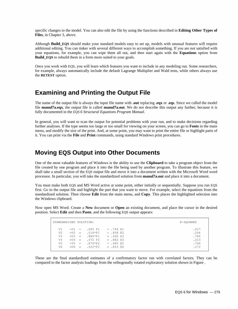
EQS 6 for Windows — 279
specific changes to the model. You can also edit the file by using the functions described in Editing Other Types of Files, in Chapter 3, above. Although Build_EQS should make your standard models easy to set up, models with unusual features will require additional editing. You can tinker with several different ways to accomplish something. If you are not satisfied with your equations, for example, you can wipe them all out, and then start again with the Equations option from Build_EQS to rebuild them in a form more suited to your goals. Once you work with EQS, you will learn which features you want to include in any modeling run. Some researchers, for example, always automatically include the default Lagrange Multiplier and Wald tests, while others always use the RETEST option.
Examining and Printing the Output File The name of the output file is always the input file name with .out replacing .eqx or .eqs. Since we called the model file manul7a.eqx, the output file is called manul7a.out. We do not describe this output any further, because it is fully documented in the EQS 6 Structural Equations Program Manual. In general, you will want to scan the output for potential problems with your run, and to make decisions regarding further analyses. If the type seems too large or too small for viewing on your screen, you can go to Fonts in the main menu, and modify the size of the print. And, at some point, you may want to print the entire file or highlight parts of it. You can print via the File and Print commands, using standard Windows print procedures.
Moving EQS Output into Other Documents
One of the most valuable features of Windows is the ability to use the Clipboard to take a program object from the file created by one program and place it into the file being used by another program. To illustrate this feature, we shall take a small section of the EQS output file and move it into a document written with the Microsoft Word word processor. In particular, you will take the standardized solution from manul7a.out and place it into a document. You must make both EQS and MS Word active at some point, either initially or sequentially. Suppose you run EQS first. Go to the output file and highlight the part that you want to move. For example, select the equations from the standardized solution. Then choose Edit from the main menu, and Copy. This places the highlighted selection into the Windows clipboard. Now open MS Word. Create a New document or Open an existing document, and place the cursor in the desired position. Select Edit and then Paste, and the following EQS output appears:
STANDARDIZED SOLUTION: R-SQUARED V1 =V1 = .645 F1 + .764 E1 .417 V2 =V2 = .514*F1 + .858 E2 .264 V3 =V3 = .885*F1 + .465 E3 .784 V4 =V4 = .472 F2 + .882 E4 .223 V5 =V5 = .874*F2 + .485 E5 .764 V6 =V6 = .522*F2 + .853 E6 .272
These are the final standardized estimates of a confirmatory factor run with correlated factors. They can be compared to the factor analysis loadings from the orthogonally rotated exploratory solution shown in Figure .

280 — EQS 6 for Windows
Running Any *.eqs File As you have now discovered, the main purpose of Build_EQS is to relieve you of the tedious details that often make developing a model harder than it needs to be. You found that you need not worry about syntax or about forgetting some key parameter that is necessary for your model to run. Choices are menu-driven and once you are familiar with the default choices (the ones that are used most often), you should become a “whiz” at EQS, clicking away like a pro! After you have constructed your basic model using the automated Build_EQS feature, in future runs you can modify and refine your model manually in your *.eqs command file. The best way to accomplish this is to edit the *.eqs file, save it, and then submit another run. If you used RETEST, then you would be editing the new file rather than the old file. (In either case, you cannot invoke Build_EQS when editing an existing *.eqs file, unless you are completely abandoning the equation structure of the model and want essentially to start over.) After you have edited and updated the file, you can run it through the Run EQS option of Build_EQS. (And don’t forget to update the model and output file names.) To illustrate the model re-specification procedure, let us make a simple modification to the manul7a.eqs file. Make this file the active window by using Window and clicking on the file name. Then, when you see the file on the screen, find the section titled /COVARIANCES, and put an exclamation mark in front of the covariance, as follows:
/COVARIANCES !F2,F1 = *;
The effect of the exclamation point is to tell EQS to ignore everything that follows it on that line. As a result, the factors will now be uncorrelated, or orthogonal. You can resubmit this job by clicking on Build_EQS and then clicking on Run EQS. The Save As dialog box will appear, and you should now change the model file name to a logical follow-up to the current name, for example, manul7b.eqs. When you make the name change, and click OK, the program will run. When it is finished, the output will come back with the output file named manul7b.out. You will find in the output file that the model with uncorrelated factors still fits the data, though not quite as well as the initial model. If you used the RETEST option of EQS, you would not edit the original file. Rather, you would edit the newly created *.eqs file, eliminating the irrelevant material and assuring that the remaining material contains the model setup that you want. RETEST is described above in the Print section.

EQS 6 for Windows — 281
8. BUILD EQS BY DRAWING A DIAGRAM It is virtually impossible to think about a complicated structural equation model, or a covariance structure model, without having a path diagram representation of the model. True, the diagram is in 1:1 correspondence to a set of equations and variance/covariance specifications, so the diagram is technically not needed. But, in reality, it is far easier to comprehend the diagram of the model than the algebraic specification of the model. Not only is a picture worth a thousand words, it is certainly worth dozens, if not hundreds, of equations! Diagrams of models are needed in both the early stages of modeling, during model conceptualization, as well as in the final stages, when one is preparing to present one's findings to the general scientific community via presentations or publications. In the early stages, a rough sketch drawn freehand may be quite adequate for personal use, but such an informal picture is inadequate for public presentation. In the past, this is where the researcher needed a graphic artist, or a commercial drawing program, in order to produce an acceptable diagram. While artists are creative, they often overlook critical features of a model that are needed for an accurate portrayal of the results. And while drawing programs are very general and can create many interesting images, their very generality means that they are not specifically tailored to the task of creating an accurate path diagram that is so critical to structural modeling. In Chapter 7, we have shown how to build an EQS model by filling in linear equation tables and various EQS commands. In this chapter you will learn how to build an EQS model by drawing path diagrams for structural equation modeling. The diagram you create is the model you run. That is, the diagram is the model input. The program translates the diagram into the algebraic language used in the model run. The diagram is also the model output, so that results are immediately available in publishable form. As a result, you can retrieve the diagram at any time, modify it, and save and print the new diagram. Because modifying an existing diagram is a minor matter, you now can produce an accurate diagram for each model that you run − giving yourself a complete record of everything you do. Furthermore, whenever you are working on any type of model that is similar to one that you have previously run, you also can retrieve your previous diagram and adjust it to be relevant to your new data or model. There is no need to start from scratch, as is now routinely, but wastefully, done.
General Overview
A path diagram contains a set of variables and specifies the connections between the variables. Hence, when you draw a diagram, you must specify the variables in your model and show the connections between them. You can draw a diagram for any model, whether this is a model that you plan to run with the EQS structural equations program or not. Because the diagram also serves as input to EQS, its initial labeling convention follows EQS. But you can modify this convention to show and print anything you want.
Variables In EQS, every variable must be one of four types: V, F, E, or D. These are the variable types available in the diagram. Typically, the relations among V and F variables represent the most important ideas in a model. A V variable is a measured variable. You can use any V designations you like, such as V345. However, if you were to use the diagram also as input to running EQS, you could use only the Vs that are actually in your data file, where
282 — EQS 6 for Windows
variables are assumed to be ordered V1, V2, ..., up to Vx, where x is the number of variables in the file. Of course, you can select among these variables, e.g., using only V3, V8, and V23 for your diagram or the model. An F variable is a hypothetical common factor that accounts for the correlation between the variables it generates. Typically, you would number Fs sequentially such as F1, F2, ... . When used in a measurement model, the observed Vs are generated by underlying Fs. Such Fs are often called first-order factors. When used in a model with higher-order factors, several Fs will be generated by one or more Fs. When the latter Fs do not directly impact on any Vs, these factors are the higher-order factors, but in general models any type of connection is possible. However, it is wise to limit your models to those that are identified and can be estimated and tested. There are also E and D variables. These are residual variables that arise automatically when Vs or Fs are dependent variables, that is, have one-way arrows aiming at them. A residual of a V variable is called an E variable, and by default the numerical part of the variable name is the same, so that (e.g.) E19 is the residual of V19. A residual in an F variable is called a D variable, and the numerical part of the name is the same.
Arrows One-way and two-way arrows show connections between variables. A one-way arrow represents a directional influence in which one variable has an effect on another variable. A one-way arrow can be interpreted as a partial regression coefficient.
A two-way arrow represents the unanalyzed correlation or covariance between variables.
Independent and Dependent Variables Every variable in your diagram that has at least one one-way arrow aiming at it is a dependent variable. Dependent variables are explained by other variables. Dependent variables cannot have covariances or two-way arrows as parameters. (If you want a dependent variable to covary with another variable, you must have its residual variable carry that covariance.) A variable that has no one-way arrow aiming at it is an independent variable. Independent variables have variances, and possibly covariances, as parameters. Only independent variables can covary with other variables, i.e., only independent variables can be connected by two-way arrows. Residual variables (Es and Ds) must be independent variables. If you want to make a residual variable a dependent variable, just change its designation to an F variable.
Free and Fixed Parameters Some parameters in a model are known ahead of time, and without looking at the data. These are called fixed parameters. If a path or covariance is not shown in the diagram, the parameter that it represents is fixed at zero. If it is shown, its value will be nonzero, typically 1.0. Other parameters are free parameters and need to be estimated with a modeling run. In the diagram, you can specify whether a parameter is fixed or free, and what its value is. The value you provide for a free parameter is called a start value.
Three Basic Model Types Assuming you follow EQS naming conventions, if your model contains only Vs and Es, you have a standard path analysis or simultaneous equation model. Such a model may contain one-way and two-way arrows.

EQS 6 for Windows — 283
If your model contains only Vs, Es, and Fs, you have a factor analysis model. Such a model is also called a measurement model. In such a model, the Fs generate the Vs via one-way arrows. If no two-way arrow connects a pair of Fs, the factor analysis model is one of uncorrelated or orthogonal factors. Otherwise, it is an oblique factor model. Typically you will have a restricted oblique factor model, one that has a lot of missing paths, and/or some zero and nonzero factor correlations. Such a model is called a confirmatory factor analysis model. If your model contains all four types of variables, you have a general linear structural equation model.
General Drawing Procedure A diagram is built from components, which are variables and the connections between them. First you must specify two or more variables. Then you can specify the arrow connections between these variables. Alternatively, you can specify a one-factor model, which will create both the variables and the arrows needed for that structure. You can add additional variables, arrows, or factor structures, or remove variables, arrows, or factor structures, at any time.
Object-Orientation Before you get started, we want to give you a way to think about the diagram. You should think of the program as an "object-oriented" program. You will find that there is a drawing screen, or diagram window, onto which you can place "objects". An object is a variable, an arrow-connection between variables, a factor structure, or any superset of these. No objects will appear in the diagram window unless you first designate the object that you desire, and then tell the program where you want that object to be. Once placed on the screen, you can manipulate these objects to achieve your goals, and in doing such manipulations, the objects will maintain their identities and characteristics (unless you purposely alter them). As examples of manipulations, you will find that once an object has been placed into a particular position in the window, it can be moved to another position. All of the characteristics of that object, such as its variable type, its name, its size, its connection to other objects, and so on, will be maintained.
Draw a model This section provides details on various drawing options (i.e., Diagrammer) you can use to construct a path diagram model. Hopefully, you already practiced a bit on the examples in Chapter 2, Quick Start. If you have not yet done so, we strongly urge you to go back to Chapter 2 for a little "hands-on" practice before getting into the details we present in this chapter. Several types of models are commonly used in analyzing data. These models are path, factor, and latent growth curve models. These models have their unique forms and can be easily defined. In order to simplify the model building process, EQS 6 has created several templates to create these models. You don’t have to physically draw the models. You only need to specify the relationship of the variables and factors; EQS will create the model in the diagram for you. You must activate Diagrammer to start to draw a diagram. The Diagrammer icon is located on the horizontal tool bar at the top of the EQS window. It is shown as Figure 8.1. You must click on it to start the diagram window.
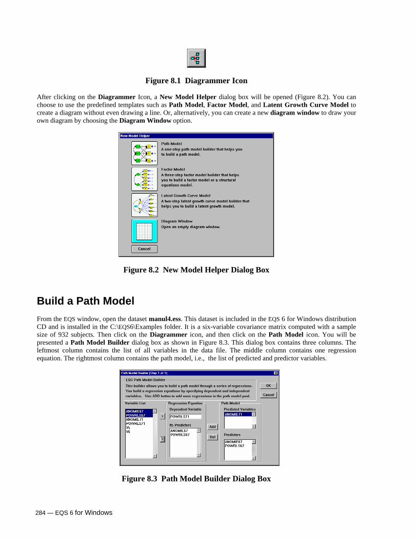
284 — EQS 6 for Windows
Figure 8.1 Diagrammer Icon After clicking on the Diagrammer Icon, a New Model Helper dialog box will be opened (Figure 8.2). You can choose to use the predefined templates such as Path Model, Factor Model, and Latent Growth Curve Model to create a diagram without even drawing a line. Or, alternatively, you can create a new diagram window to draw your own diagram by choosing the Diagram Window option.
Figure 8.2 New Model Helper Dialog Box
Build a Path Model From the EQS window, open the dataset manul4.ess. This dataset is included in the EQS 6 for Windows distribution CD and is installed in the C:\EQS6\Examples folder. It is a six-variable covariance matrix computed with a sample size of 932 subjects. Then click on the Diagrammer icon, and then click on the Path Model icon. You will be presented a Path Model Builder dialog box as shown in Figure 8.3. This dialog box contains three columns. The leftmost column contains the list of all variables in the data file. The middle column contains one regression equation. The rightmost column contains the path model, i.e., the list of predicted and predictor variables.
Figure 8.3 Path Model Builder Dialog Box

EQS 6 for Windows — 285
A path model is also called a simultaneous equation model. It consists of a number of regression equations with some correlations among independent variables. The unique feature of a path model is that all the variables used in the model are measured variables. There are four steps to using this dialog box.
Step 1: Specify a dependent variable from the variable list on the left hand side of dialog box, and click on the top button to move the variable to the Dependent Variable list box.
Step 2: Select the independent variables from the variable list box and move them to the Its Predictors
list box (if you want to select several non-contiguous variables, press down the CTRL key and click on the variables in the variable list box).
Step 3: Click on the Add button to move the regression equation to the Path Model section on the right
hand side. Step 4: Repeat steps 1 - 3 until all regression equations are moved to the Path Model section. You have
completed the process of building a path model. These equations are your path model. Click on the OK button; EQS will open a diagram window and put the path model you have specified in the window (see Figure 8.4).
Our path model has two equations:
ANOMIE71 = *ANOMIE67 + *POWRLS67 + error; POWRLS71 = *ANOMIE67 + *POWRLS67 + error;
To build this model, we first click on ANOMIE71 and move it to the Dependent Variable box. Then we select ANOMIE67 and POWRLS67 and move them to the Its Predictors list. The first equation is complete so we click on the Add button, and the first equation is moved to the Path Model section. For the second equation, we click on the POWRLS71 and move it to the Dependent Variable box. Again, we select ANOMIE67 and POWRLS67 and move them to the Its Predictors list box. This stage of building the model is shown in Figure 8.3. Click on the Add button to add the second equation to the Path Model section. The path model building process is complete and we click on the OK button. The model is created as shown in Figure 8.4.
Figure 8.4 Path Model Created by New Model Helper The path model has been built using the Diagrammer with very little effort. You are ready to run EQS based on the model you just built.
Build Path Model Command File To build the EQS model from the diagram shown in Figure 8.4 you need just a few more clicks. While on the diagram window (please note that both your data and diagram are active at this point), pull down the Build_EQS menu and select Title/Specifications. First, you will be prompted to save the diagram and then the EQS Model Specifications dialog box (Figure 8.5) will appear. In the dialog box, the data file name has been filled in and the

286 — EQS 6 for Windows
default estimation method is given. Most of the model’s input information has been provided. You are ready to obtain the EQS model listing by clicking on the OK button. After clicking on the OK button, a text window will be created and a text file as shown in Figure 8.6 will be displayed in it. This is the file of EQS model commands created for you from Diagrammer; it is ready to run. Go back to the Build_EQS menu, pull it down and select the Run EQS option to run it.
Figure 8.5 EQS Model Specifications Dialog Box
/TITLE EQS model created by EQS 6 for Windows /SPECIFICATIONS DATA='c:\eqs61\examples\manul4.ess'; VARIABLES=6; CASES=932; GROUPS=1; METHODS=ML; MATRIX=CORRELATION; ANALYSIS=COVARIANCE; /LABELS V1=ANOMIE67; V2=POWRLS67; V3=ANOMIE71; V4=POWRLS71; V5=V5; V6=V6; /EQUATIONS V3 = + *V1 + *V2 + 1E3; V4 = + *V1 + *V2 + 1E4; /VARIANCES V1 = *; V2 = *; E3 = *; E4 = *; /COVARIANCES V2 , V1 = *; /PRINT EIS; FIT=ALL; TABLE=EQUATION; /STANDARD DEVIATION /MEANS /END
Figure 8.6 Path Model Command File Built by Build_EQS Process
Before EQS runs the model, you will be asked to save the model file in a dialog box shown as Figure 8.7. You have to save the model file for EQS to continue.

EQS 6 for Windows — 287
Figure 8.7 Save As Dialog Box
After you click on the Save button, EQS will start to run. Depending on the speed of your computer, EQS will display its running status until it finishes. The EQS output will be displayed in the front window for you to examine. We will not show EQS output here. Detailed information on EQS output is provided and illustrated in the EQS 6 Structural Equations Program Manual.
Build a Confirmatory Factor Analysis Model
Let’s build a confirmatory factor analysis model using a raw score dataset called manul7.ess, which is stored as an EQS system file. This dataset is included in the EQS 6 for Windows distribution CD and is installed in the C:\EQS6\Examples folder. This data file has six variables. We want to show you how to build a six-variable, two-factor confirmatory factor model (CFA). We will develop the model based on the raw data. If the file were the covariance or correlation matrix for these data, we would use a virtually identical procedure.
Note: If you prefer, you can use manul7a.ess rather than manul7.ess. Manul7a.ess is nearly identical to
manul7.ess, but one case containing an outlier is deleted.
Select Diagrammer. From the New Model Helper (shown in Figure 8.2), click on the second picture button labeled Factor Model. You will see a series of dialog boxes to create a factor model. These dialog boxes are
1. Dialog box to acquire all factor structures 2. Dialog box to specify all structural equations 3. Dialog box to specify all factor correlations
The first dialog box is EQS Factor Structure Builder (Figure 8.8). It allows you to define all factor structures by specifying their indicators. The dialog box consists of three columns. The leftmost column contains the list of all variables in the data file. The middle column contains the factor structure of one factor, and the rightmost column contains the list of model components. You create a factor structure by moving its indicators to the list box labeled Indicators. When one factor is done, you click on Add, which adds it to the Model Components section on the right. Repeat this process until all factor structures are created. In this example, you will select V1, V2, and V3 and click on the right arrow button to move them to the indicator box. Click on the Add button to create the first factor structure. Next, select V4, V5, and V6, move them into the indicator list (this stage is represented in Figure 8.8) and click on the Add button to create the second factor structure. Click Next to move to the next step.
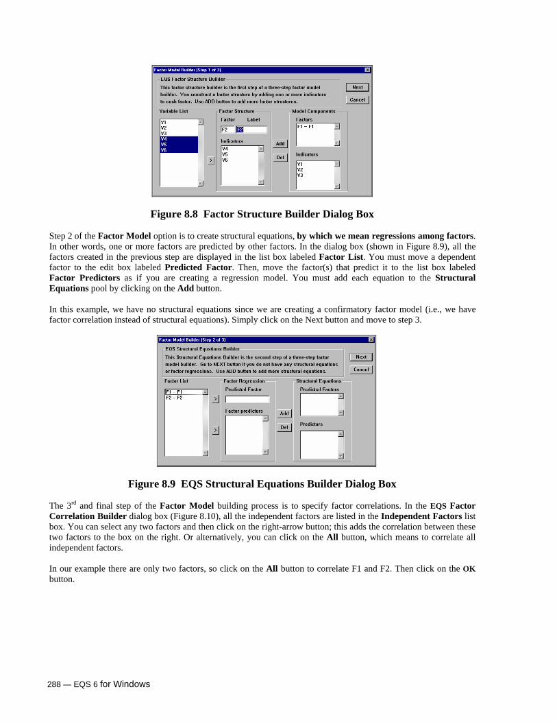
288 — EQS 6 for Windows
Figure 8.8 Factor Structure Builder Dialog Box
Step 2 of the Factor Model option is to create structural equations, by which we mean regressions among factors. In other words, one or more factors are predicted by other factors. In the dialog box (shown in Figure 8.9), all the factors created in the previous step are displayed in the list box labeled Factor List. You must move a dependent factor to the edit box labeled Predicted Factor. Then, move the factor(s) that predict it to the list box labeled Factor Predictors as if you are creating a regression model. You must add each equation to the Structural Equations pool by clicking on the Add button. In this example, we have no structural equations since we are creating a confirmatory factor model (i.e., we have factor correlation instead of structural equations). Simply click on the Next button and move to step 3.
Figure 8.9 EQS Structural Equations Builder Dialog Box
The 3rd and final step of the Factor Model building process is to specify factor correlations. In the EQS Factor Correlation Builder dialog box (Figure 8.10), all the independent factors are listed in the Independent Factors list box. You can select any two factors and then click on the right-arrow button; this adds the correlation between these two factors to the box on the right. Or alternatively, you can click on the All button, which means to correlate all independent factors. In our example there are only two factors, so click on the All button to correlate F1 and F2. Then click on the OK button.

EQS 6 for Windows — 289
Figure 8.10 EQS Factor Correlation Builder Dialog Box
You will see a diagram window containing a two-factor CFA model (Figure 8.11). You are ready to run this model.
Figure 8.11 Two Factor CFA Model
Build Factor Model Commands
After you have opened the data file and drawn the diagram, you are ready to build the EQS model. Click the Build_EQS selection from the main menu. You can see from the drop-down menu that there are many items in this menu, but only two are active. The active options are black, while the inactive options are grayed out. This choice of only two options indicates that you should start with the item on top of the menu, Title/Specifications, to build an EQS model. By selecting this option, you will see the EQS Model Specifications dialog box (Figure 8.12). But before it appears, you will be asked to save the diagram.
Note: EQS 6 uses FACMOD.EDS as the default diagram file name. You may want to save this diagram as MANUL7.EDS since this name coincides with your data file name.

290 — EQS 6 for Windows
Figure 8.12 EQS Model Specifications Dialog Box This dialog box contains the information that is needed in the /SPECIFICATIONS section of the EQS program. You can see that it already has most of the information you need to specify a model. Some of the default information is from the *.ess file (here, manul7.ess), and some reflects choices typically made in structural modeling. We now present a new option that you may find useful. EQS can display its output in HTML format like the documents you read on the World Wide Web. It also has a built-in HTML file viewer that allows you to go to an exact section of EQS output. To turn on this HTML option, click on the Misc. Options button in the dialog box above. The Additional /SPECIFICATION options dialog box will appear (Figure 8.13). In the Type of output file group, select the HTML file option, then click the Continue button to close this dialog box. You will be returned to the dialog box in Figure 8.12. Click the OK button to close it. You will see the EQS model instructions in a text window. You are now ready to run EQS.
Figure 8.13 Additional /SPECIFICATION Options Dialog Box

EQS 6 for Windows — 291
EQS Model File Whether or not you build your model from a diagram or an equation table, you finish building an EQS model with the Build_EQS feature. As this is done, you can see that the EQS command language is built line by line and is written onto the background window. The file is called manul7.eqx by default because the name of the diagram file is manul7.eds. We use .EQX as the EQS model file extension. Detailed model information is saved in this file. When the cursor returns to the manul7.eqx window, your model is complete, and you are ready to run EQS. The following shows part of the model file that is created.
/TITLE EQS model created by EQS 6 for Windows /SPECIFICATIONS DATA='c:\eqs61\examples\manul7.ess'; VARIABLES=6; CASES=50; GROUPS=1; METHODS=ML; OUT=HTML; MATRIX=RAW; ANALYSIS=COVARIANCE; /LABELS V1=V1; V2=V2; V3=V3; V4=V4; V5=V5; V6=V6; /EQUATIONS V1 = + 1F1 + 1E1; V2 = + *F1 + 1E2; V3 = + *F1 + 1E3; V4 = + 1F2 + 1E4; V5 = + *F2 + 1E5; V6 = + *F2 + 1E6; /VARIANCES F1 = *; F2 = *; E1 = *; E2 = *; E3 = *; E4 = *; E5 = *; E6 = *; /COVARIANCES F2 , F1 = *; /PRINT EIS; FIT=ALL; TABLE=EQUATION; /END
If you need to change the model file or add to it, you must go to the Build_EQS menu and select the appropriate menu for your options. After you make changes, the EQX file window will be re-drawn to include the changes. Notice that this window cannot be edited directly. All the changes to the EQS model must be done in relevant dialog boxes.

292 — EQS 6 for Windows
Build a Latent Growth Curve Model We will open the wisc.ess data, which you can find in the EQS 6 example folder. The data consist of WISC scores collected at four time points, and mothers’ education. This study was carried out by Osborne between 1961 and 1965 (Osborne & Suddick, 1972)44. The growth of WISC has a linear trend. Before running a Latent Growth Curve Model, you must make the following decisions:
1. Choose the variables to be used and their time lines. 2. Choose from three model options and decide on growth factors.
A typical Latent Growth Curve (LGC) model consists of one or more growth factors and one intercept factor. In the case of linear growth, there is only one linear growth factor. If the data has a quadratic growth trend, the model will have two growth factors, for quadratic and linear growth. Likewise, if you theorize that the model has cubic growth, there will be three growth factors, namely cubic, quadratic, and linear growth. Finally, if you theorize that the model has quartic (fourth-power) growth, there will be four growth factors, namely quartic, cubic, quadratic, and linear growth. The template allows you to specify only measured variables as test variables. If you have some latent variables or factors to be used as test variables, you must build the LGC model, then customize it manually. The EQS Diagrammer makes this quite easy to do. Let’s start our LGC model using the WISC dataset. You must first open the dataset and click on the Diagrammer icon (as shown in Figure 8.1) from the horizontal tool bar. The New Model Helper will appear (Figure 8.2). Click on the third picture icon from the top, labeled Latent Growth Curve Model. A dialog box will appear as shown below (Figure 8.14). All the variables are presented in the list box labeled Variable List. You must choose those variables to be included in the model and use the right arrow button to move them into the list box labeled Variables Deployed.
Figure 8.14 First Step of Latent Growth Curve Model When you click on a variable in the Variables Deployed list, you will see the default time appear in the edit box labeled Time line for this measurement. You may change the value in the edit box by double-clicking in it, then typing the desired value. Default time for the first variable deployed is 1, for the second is 2, etc. In this case, WISC_1 is measured in the first year, WISC_2 is measured in the second year, WISC_3 is measured in the fourth year, and WISC_4 is measured in the sixth year. Change the time line of WISC_3 to 4, and change the time line of WISC_4 to 6 (as in Figure 8.14).
Note: Failure to provide correct time lines of each test variable will result in incorrect coefficients of
growth factors.
44 Osborne, R. T., & Suddick, D. E., 1972. A longitudinal investigation of the intellectual differentiation hypothesis. Journal of Genetic Psychology, 121, 83-89.

EQS 6 for Windows — 293
Note: If you change any time lines, hit the <Enter> or <Tab> key before clicking on Continue.
After clicking on Continue, you will see the dialog box shown in Figure 8.15. In the group box labeled Latent Growth Curve Model Options, there are three choices:
Initial Status Model Each value in the X column is calculated from the time for that variable by subtracting the time for the first variable. This is the typical choice. In this example, the times for the four variables are 1, 2, 4, and 6, so the X-values would be 0, 1, 3, and 5.
Time Averaged Model Each value in the X column is calculated from the time for that variable by subtracting the mean time for all variables, so that the mean of the X’s will be zero. When computing the coefficients of the Time Averaged Model, we use the method of orthogonal polynomial coefficients. This example is shown in Figure 8.15.
Linear Spline Model Values in the X column are calculated from the means of the test variables. If the dataset is a covariance or correlation matrix file, it must include the variable means.
In this example, we choose Time Averaged Model as the method to construct the LGC model. As you can see from the X column in the middle of the dialog box, the coefficients are -2.25, -1.25, 0.75, and 2.75 respectively for the linear growth factor. The table also shows the orthogonal polynomial coefficients for quadratic, cubic, and quartic growth. At the lower part of the dialog box, there are four large picture buttons. If you have five or more variables, there will be another picture button labeled Quartic. Click on the growth curve that fits your data. Since the WISC data shows linear growth, we click on the button on the far left, which shows linear increment or decrement.
Figure 8.15 Second Step of Latent Growth Curve Model
After you click on the picture button for linear growth curve, a diagram representing the LGC model will appear in the diagram window (Figure 8.16). Note that there are two factors in the diagram. One is called Linear Growth Factor and the other is called Intercept Factor. Each factor has four blue one-way arrows pointing to the measured
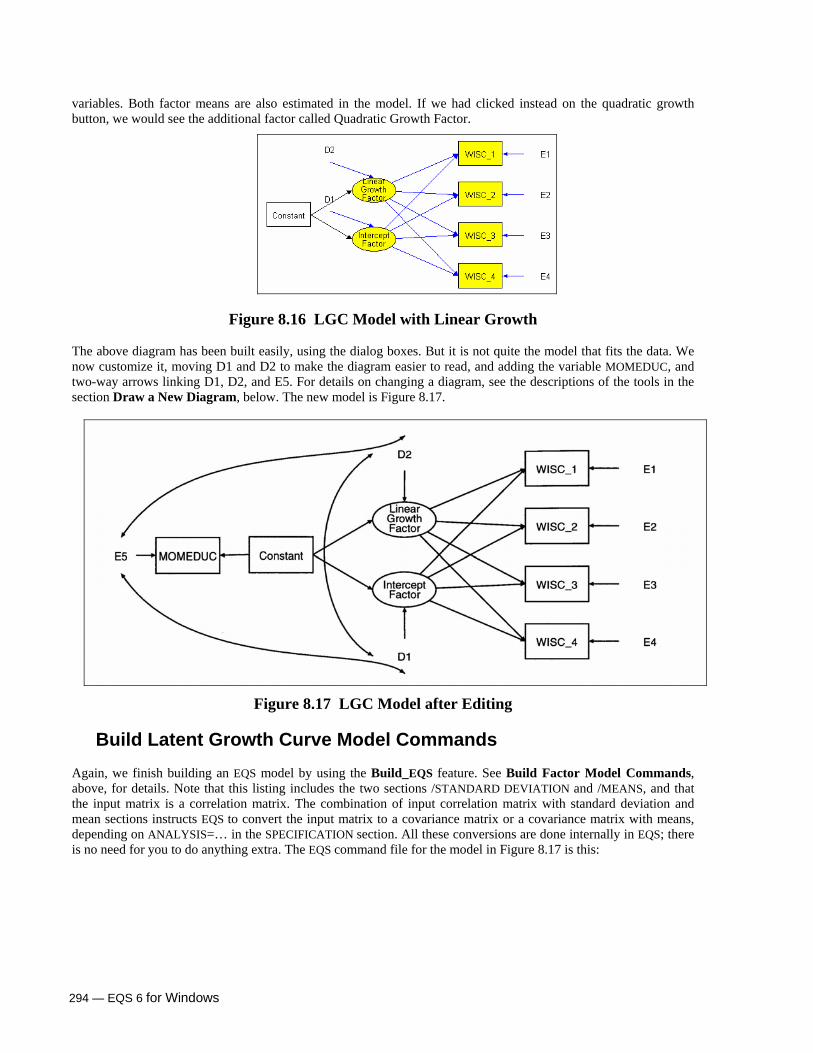
294 — EQS 6 for Windows
variables. Both factor means are also estimated in the model. If we had clicked instead on the quadratic growth button, we would see the additional factor called Quadratic Growth Factor.
Figure 8.16 LGC Model with Linear Growth
The above diagram has been built easily, using the dialog boxes. But it is not quite the model that fits the data. We now customize it, moving D1 and D2 to make the diagram easier to read, and adding the variable MOMEDUC, and two-way arrows linking D1, D2, and E5. For details on changing a diagram, see the descriptions of the tools in the section Draw a New Diagram, below. The new model is Figure 8.17.
Figure 8.17 LGC Model after Editing
Build Latent Growth Curve Model Commands
Again, we finish building an EQS model by using the Build_EQS feature. See Build Factor Model Commands, above, for details. Note that this listing includes the two sections /STANDARD DEVIATION and /MEANS, and that the input matrix is a correlation matrix. The combination of input correlation matrix with standard deviation and mean sections instructs EQS to convert the input matrix to a covariance matrix or a covariance matrix with means, depending on ANALYSIS=… in the SPECIFICATION section. All these conversions are done internally in EQS; there is no need for you to do anything extra. The EQS command file for the model in Figure 8.17 is this:

EQS 6 for Windows — 295
/TITLE EQS model created by EQS 6 for Windows -- c:\eqs6\examples\gwlinear.eds /SPECIFICATIONS DATA='c:\eqs61\examples\wisc.ess'; VARIABLES=5; CASES=204; GROUPS=1; METHODS=ML; MATRIX=CORRELATION; ANALYSIS=MOMENT; /LABELS V1=WISC_1; V2=WISC_2; V3=WISC_3; V4=WISC_4; V5=MOMEDUC; /EQUATIONS V1 = + 1F1 + -2.25F2 + 1E1; V2 = + 1F1 + -1.25F2 + 1E2; V3 = + 1F1 + 0.75F2 + 1E3; V4 = + 1F1 + 2.75F2 + 1E4; V5 = + *V999 + 1E5; F1 = + *V999 + 1D1; F2 = + *V999 + 1D2; /VARIANCES V999 = 1.00; E1 = *; E2 = *; E3 = *; E4 = *; E5 = *; D1 = *; D2 = *; /COVARIANCES D1 , E5 = *; D2 , E5 = *; D2 , D1 = *; /PRINT EIS; FIT=ALL; TABLE=EQUATION; /STANDARD DEVIATION /MEANS /END
Draw A New Diagram In addition to the three easy-to-use templates in the Diagrammer option New Diagram Helper dialog box, there is another picture, namely Diagram Window. If you have a diagram that is too complex for the templates, the Diagram Window option allows you to create a diagram by free style drawing. Click on the picture button labeled Diagram Window from the New Diagram Helper, and you will see an empty diagram (Figure 8.18). There is a vertical toolbar on the left side of the window and there are some areas designated with cyan color, where you cannot draw. The white area is for drawing your diagram.

296 — EQS 6 for Windows
Figure 8.18 New Diagram Window The vertical tool bar on the left side gives you all you need to draw a diagram. As you can see, there are 15 picture buttons in the tool bar. The first two buttons each have a special purpose. Each of the other 13 buttons causes an object to be created. These buttons can be categorized as referring to three types of objects:
1. Variables of several types 2. Connections between variables, also of several types 3. Shortcut buttons which create more than one of the above
A path diagram contains a set of variables and specifies the connections between the variables. Hence, you must first specify the variables in your model and then show the connections between them. Usually, you will first specify two or more variables. Alternatively, you can specify a one-factor model, which will create both the variables and the connections between variables needed for that structure. At any time, of course, you can add additional variables, additional connections, or additional factor structures, or remove variables, connections, or factor structures. To draw a variable object (i.e., V, F, E, D, and factor structure), you must click the icon on the tool bar. Then, move your mouse pointer to the diagram window, where the cursor’s position will be indicated by a small rectangle, with a plus sign just to the left of it. Move the mouse so that the plus sign is where you want the upper left corner of the object to be located. Then click the mouse again, and the object will appear there. Of course, you can always change the position of an object after you have drawn it. The fifteen buttons have specific functions as explained next.
A. Reset Tool This tool is very important, because it ends the action of any other tool. Suppose that you have drawn all the V variables in your diagram, and now want to do something else. If you click anywhere in the diagram, you will create another V variable, which you do not want to do. Instead, click on this reset tool (or right-click on your mouse), which resets the Diagrammer. Now you can continue with the next step in drawing your diagram.

EQS 6 for Windows — 297
B. Text Tool This tool is used to add text to the diagram, e.g. explanatory titles and labels. Click on it, and then move your mouse until the cursor is where you want to add the text. Click, and type your text. Text will appear in the default font and size, which you can modify. You can also use the click-and-drag procedure to move the text to any location.
C. One-way Arrow A "causal" relationship is shown as a one-way arrow between two variables, with the direction of the arrow representing the direction of hypothesized causation. A one-way arrow from an F to a V is used to represent a factor loading in a measurement model. More generally, a one-way arrow represents the coefficient, or weight, used in the prediction of one variable from another variable. These one-way arrows, or coefficients, are sometimes called path coefficients. In EQS, one-way arrows can only aim at V and F variables. Whenever you aim an arrow at a variable, it becomes a dependent variable that has its own residual. The diagram creates these residuals automatically. Visually, a one-way arrow is a straight line with an arrowhead endpoint. If you move one or both of the variables connected by a one-way arrow, the arrow will move so that the points remain connected.
D. Two-way Arrow Only two independent variables can be connected by a two-way arrow, which represents a covariance or correlation between these variables. In general, you should connect only those variables that make sense to be connected. Remember that you cannot correlate a dependent variable with any other variable, so you cannot connect a two-way arrow to a variable that also has a one-way arrow aiming at it. If you want to do something like this, go to the residual variable associated with the dependent variable. It will be an independent variable, and can be correlated with any other independent variable. (But such a model can be tested only if it is identified!) Visually, a two-way arrow is a straight line that has arrowheads at both ends, connecting two variables. If you move one or more of the variables, they will remain connected by the straight line with arrowheads.
E. V-type Variable — A Measured Variable Variables designated by the letter V are measured or observed variables. These are the variables in your data file, and, as such, are typically numbered sequentially V1, V2, ..., up to the number of variables in your file. Not all of these variables need to be in your diagram, nor in any model you run. A model with only V and E variables is a path analysis or simultaneous equation model. A model with no V variables cannot be tested against data.
298 — EQS 6 for Windows
F. F-type Variable — A Factor A factor, or F variable, represents the common variance shared between the variables that it aims at. If an F variable aims at V variables only, it is a first-order common factor, a regular factor of factor analysis. It accounts for the correlations among the V variables. Of course F variables may themselves be correlated, as shown by two-way arrow connections. When these two-way arrows are removed, and another F variable is hypothesized to account for these correlations, this new F variable having one-way arrows aiming from it toward other Fs is a higher-order factor. Generally the name "higher-order factor" implies that this F has no one-way arrows aiming at Vs, but there is no special reason for such a restriction.
G. E-type Variable — An Error Variable Whenever an arrow aims at a V variable, making it a dependent variable, a residual E variable will be added to aim at that same V variable. Thus E15 goes with V15. An E variable represents variance in the V variable that cannot be explained by the predictors of the V variable. E variables must be independent variables. Thus they may correlate with other independent variables, but they cannot have one-way arrows aiming at them. If you want to achieve the effect of making an E variable a dependent variable, just change its name from an E variable to an F variable. When you add an arrow pointing at the F variable, EQS will add a residual to the F variable, namely, a new D variable.
Note: In general, you do not need to create or draw E variables. These are created automatically. Only in special models will you need to add or remove E variables.
H. D-type Variable — A Disturbance Variable Whenever an arrow aims at an F variable, making it a dependent variable, a residual D variable will be added to aim at that same F variable. Thus D5 goes with F5. A D variable represents variance in the factor that cannot be explained by that factor's predictors. If the predictors cannot explain any variance in the factor, the D variable is synonymous with the factor. D variables must be independent variables. Thus they may be connected to other variables by two-way arrows, and they cannot have one-way arrows aiming at them.
Note: In general, you do not need to create or draw D variables. These are created automatically. Only in special models will you need to add or remove D variables.
I. Factor Structure A factor structure is a completely drawn path diagram for a one-factor model with its indicators. It contains one F variable and as many V variables as you designate, as well as the associated errors in variables (Es). When creating a factor structure, you can specify a regular factor loading, a slope for an LGC model, or a constant for an LGC model.
EQS 6 for Windows — 299
J. Curved One-way Arrow A curved one-way arrow connecting two variables is identical in meaning to a straight one-way arrow. Only the graphical representation differs. A pleasing curved line is used to connect the two variables. If you move one of the variables connected by a curved one-way arrow, the one-way connection stays and remains curved.
K. Curved Two-way Arrow A curved two-way arrow connecting two variables has the identical meaning as an ordinary, straight two-way arrow connecting two variables. Visually, however, the connection is smoothed and curved. If you move one of the variables connected by a curved two-way arrow, the connection stays and remains curved.
L. 999 Variable — A Constant Variable This option allows you to place a constant or intercept variable on the diagram window. This constant variable is essential for covariance structures with means, or latent growth curve models.
M. Regression Tool A regression tool connects several measured variables or factors to a designated measured variable or factor. You have to deploy all the variables you want to connect before using this tool.
N. Factor Loading Tool A factor loading tool connects one factor to several measured variables or factors having related error or disturbance variables. It is similar to the factor structure tool to create a factor structure. Unlike the factor structure tool, which creates the structure through a dialog box, you have to deploy all factors and measured variables before you can use this tool.
O. Covariate Tool A covariate tool connects all possible covariates among the independent variables.
Some Suggestions for Good Results Before you draw many diagrams, you should try to study path diagrams published by your favorite authors. What is it that makes a good diagram, i.e., one that communicates easily and accurately, and is also pleasing to the eye? There are a lot of principles, but among the important ones are:

300 — EQS 6 for Windows
• There is a logical organization to the picture, e.g., causal flow is all in one direction. • There is balance and harmony in the diagram. • Variables are placed so as to minimize the occurrence of lines crossing other lines. • Relative size and location of variables is meaningfully thought out. • Labeling of variables is clear and self-explanatory. • Not too much information is placed into one diagram. Most of these principles are obvious, but you have to remember that what is obvious to you may not be obvious to your reader or audience. If some variables are shown larger than others, does that mean they are more important than others? If the causal flow appears to be in all directions, does that mean that nothing systematic is going on? Don't forget that if your diagram is incomprehensible to your readers, your explanations of the diagram are liable to be even more incomprehensible to them. Of course, even the best visual presentation of a complicated model may be too difficult for some readers. You should remember that there is no reason to think that a model must be presented in a single diagram. In a very complicated model, it may be helpful to the reader to see the model presented in several diagrams rather than one. For example, one diagram could show the measurement model, and another could show the relations among latent variables. And some aspects of the model, perhaps, are best described in text and not shown in the diagram at all! The diagram permits you to create your actual model (which may be quite complex), and then to visually present only selected aspects of that model. Although Diagrammer is very flexible, and permits you to draw any almost any kind of diagram, it is good practice to follow a set of rules every time you use the program. We will give our suggestions for these rules, but you may also develop your own. A standard set of rules will help you to organize your diagram to minimize potential mistakes, give you pleasingly consistent results, and assure that the diagram works properly. In addition, when using the diagram as your actual model specification for an EQS run, these rules will help ensure that the model is set up correctly. Here are our suggestions for good drawing practice:
1. Use a subset of your data file so that all the variables will be used. 2. Use the variables in sequence from small to large (i.e., start with V1). 3. To create a factor structure, use the Factor Button below. 4. Do not draw E (error) and D (disturbance) variables. They will be generated automatically. 5. Lay out all factor structures and measured variables and align them, before connecting them. 6. Use the ordinary straight one-way arrow to draw a regression path. 7. Use the curved two-way arrow to connect two independent variables.
A complete diagram will require the use of many of the tools provided in Diagrammer. Although we could start our exposition with elementary tools, let us start with a tool that will help us to build a large structure quickly.
Create a Factor Structure with the Factor Button One of the most common parts of a covariance structure model is a factor with its indicators. While a model may contain many factors, each with its own indicators, the complete diagram is best built one factor at a time. The simplest way to do this is with our factor button in the list of diagram drawing tools. Later we will show you how to achieve the same effect based on the non-modular method, in which the complete structure is built from small parts. The latter approach is important because it will teach you diagramming elements that will be helpful in many situations.

EQS 6 for Windows — 301
A factor loading structure consists of one factor, its several measured variable indicators, and the errors in the variables. A typical example is the four-variable, one-factor structure in Figure 8.19. Here, and in the rest of this section, we use the dataset ability.ess, which is included on the EQS distribution CD.
Figure 8.19 One Factor with Four Indicators As you can see, F1 generates the Vs, so the arrows go from F1 to the Vs. Each V also is influenced by its own residual error variable. Visually, this diagram uses the standard convention of putting latent variables into circles or ovals, and measured variables into squares or rectangles. The diagram provides an easy way to create such a structure. Click on the factor structure icon, which is the ninth of the fifteen tool icons on the left side of Figure 8.18. Next, move the mouse pointer to the approximate position in the diagram window where you want to place the structure, and click the mouse pointer again. A Factor Structure Specification dialog box like Figure 8.20 or 8.21 will appear. When there is a data file available and opened, you will get the dialog box in Figure 8.20.
Figure 8.20 Factor Structure Specification Dialog Box with Data File Opened
Figure 8.21 Factor Structure Specification Dialog Box without Data File Opened

302 — EQS 6 for Windows
This dialog box is all you need to specify a factor loading structure. To complete the dialog box, you must enter the factor name (or use the default), fill in the factor label, specify the indicators of the factor, and possibly customize some aspects of the specifications. We will describe each of dialog box elements in turn.
Factor Name In the top part of the dialog box, a new factor number (i.e., F1) has been given as the default. If this is indeed your F1, there is nothing you need to do. However, if you want this particular factor to be (say) F12, you would need to change the default designation.
Factor Label Below the factor number, you can enter the factor label. This is a mnemonic designation that will remind you and your readers about the interpretive meaning of the factor. If you do not have many factors and variables in your diagram, you can get away with quite a long label, but if you are planning to cram a lot of visual material into a small amount of space, you should consider using short labels. The factor label cannot exceed 32 characters in length. Remember that a long label will require quite a lot of space. It is possible that your circle may be too small for such a long label, and it may be necessary to increase the size of your circle. If you want your factor label to appear on more than one line, you must decide where the line breaks should be. At the point of the break, you must enter a semi-colon ";" character between the words.
Specify Factor Indicators
With Data File Opened As shown in Figure 8.20, all the variables in your dataset will be presented in the Variable List box. Keeping this list short is one reason to limit your dataset to the variables that you plan to use in the model. To create a factor structure, you must move target variables from the Variable List box to the Indicator List box. You do this by first selecting all the relevant variables in the Variable List.
Note: If you need to select non-contiguous variables from the list, hold down the <CTRL> key (known as the control key) while you use your mouse to click on the target variables.
After you have selected all the variables in a desired factor structure, click on the right arrow button to move all the selected variables to the Indicator List. If you change your mind, you can modify the choice of variables by moving one or more variables back to the Variable List from the Indicator List by using the left arrow button. You can move variables back or forth, as you like. When a variable is used in another part of the diagram, this variable will not appear in the Variable List again to avoid mistakes.
Without Data File Opened In this section, all the discussions refer to the dialog box in Figure 8.21. There are two ways to specify the Vs that you intend to have as indicators of this factor. These two ways correspond to choices given by the two radio buttons. The first button permits you to select Vs from a sequential set of variables. The second button permits you to skip around and select variables arbitrarily.
EQS 6 for Windows — 303
Sequential Indicators
The first button provides a list of sequential indicators that is shown in Figure 8.21 as V1 to V3. You can substitute any beginning variable for V1, and any ending variable for V3. Click the APPLY button when you have entered your beginning and ending Vs. As a result, the changes you made will be applied to the list box shown in the bottom left, under the Indicator Specifications.
Selected Indicators
If the Vs that you want to use are not sequential, you have to select the second radio button marked Indicator List. An edit box will appear to the right. Type the names of the indicator variables in the edit box, using commas to separate them. As an example, you might type: V1,V6,V13,V14. After the indicators are entered, click the APPLY button. This places the Vs that you typed into the list box shown in the bottom left under the Indicator Specifications.
Parameter Types, Start Values, and Labels On the bottom of the dialog box (Figure 8.20 or 8.21), there is a group box called Indicator Specifications. Some options in this box permit you to specify information about variables and parameters.
Free and Fixed Factor Loadings By default, each factor loading is considered to be a free parameter. That is, all paths from the factor to its V indicators are assumed to be free to estimate. To make one of the factor loadings fixed rather than free, you have to highlight an indicator by clicking on its name in the List box. Then, click on the Fixed Parameter radio button. To make a fixed parameter free, you would mark the variable in the list and choose Free Parameter instead.
Start Value EQS supplies default start values for free parameters. If you wish, you may override one or more start values. This is advisable if you have a good guess as to the final parameter value, e.g. from an EQS run on a similar model. To supply a start value, type it in the edit box when the relevant V variable is highlighted.
Note: You can double-click on any parameter object (i.e., independent variables and all parameters) to specify the start value of a parameter.
Variable Label Without further designation, Vs are just Vs. If you want to add a label to one of the indicators, you must double-click on the indicator name in the list box. A Measured Variable Specification dialog box like the one shown in Figure 8.28 (below) will appear. Basically, that dialog box permits you to enter a label of at most 32 characters to describe the chosen V variable.
OK or Cancel When you have completed your choices in the Factor Structure Specification dialog box, or if you have made no choices but are happy with the defaults, you must press the <ENTER> key or click OK to have the program draw the factor structure. If you change your mind about your specifications, just press Cancel.

304 — EQS 6 for Windows
Create a Factor Structure Using Individual Objects Although most of the time we recommend using the above procedure to draw a factor with its indicators in one quick operation, you should still learn how to use the individual objects in the tool bar. You will certainly have occasion to use most of them. We shall now create the above factor structure element by element, using a series of steps. As you can see from the diagram in Figure 8.19, to construct such a structure you will need to draw four rectangles to represent the four Vs (indicators), one circle or oval to represent the factor, and four one-way arrows to represent factor loadings. EQS will automatically supply four Es to represent the error variables, and four error paths. After the structure is drawn, you can customize the structure by inserting variable labels, etc. You will be placing each of these model components on the screen, one by one, in the location that you specify. If the spacing and alignment of the components is not perfect, do not worry. The program provides editing tools that permit you to balance and beautify your diagram. The sequence of steps needed to create the four variable factor loading structure is given next. We suggest that you work our example on your computer. First, open the dataset ability.ess.
Deploy Indicators on Diagram Window EQS distinguishes whether a data file is opened when you deploy indicators on the diagram window.
When Data file is opened To deploy indicators on the diagram window, you click on the vertical tool bar icon that represents a V variable (the fifth icon on the left side of Figure 8.18). You will be asked if you want to deploy more than one variable in the diagram window. If you answer No to this question, you will be able to place variables sequentially without selection. Move your mouse cursor to the diagram window. Your mouse cursor will turn to a cross with a small rectangle attached to its lower right. Then, you are ready to deploy measured variables: with every click on the diagram window, one measured variable will be put on the screen. You can see that these variables are deployed according to their sequence in the data. Click on the YES button if you want to select variables to place into the draw window. A second dialog box will appear, as shown in Figure 8.22.
Figure 8.22 Deploy Measured Variables Dialog Box

EQS 6 for Windows — 305
Select the variables you want to use in the model, then click on the right arrow button. The variables you have just selected will move to the list box Variables to Use. You must verify that these variables are the ones that you want to use in the model. If they are correctly chosen, click on the OK button to deploy the variables onto the diagram window. If not, select variables and use the right arrow and left arrow keys to move the variables into their correct position. Then click OK. The variables are always deployed at the upper left corner of the window to avoid other drawing objects. You must move them to appropriate locations in the window. The deployed variables are show as Figure 8.23.
Figure 8.23 Deployed Variables
When data file is not opened When a data file is not available or is not opened, you only need to click on the button, move the mouse cursor to the diagram window and click four times. Four variables will be deployed on the window. The variable names will be sequential such as V1, V2, etc. Since no data file is opened, the variable labels will be identical to variable names.
Deploy a Factor on Draw Window Click the F variable once and move the mouse pointer to the appropriate location of the diagram window and click once. The factor creation status will remain until your turn it off. To reset the mouse cursor, you must click the reset button (top icon on the left of Figure 8.18), or click the right mouse button once anywhere in the window.
Connect All The Variables Using Factor Tool After all the variables in a factor structure are deployed, arrange them neatly so that the structure will look nice. Figure 8.24 is an example of the variable layout.
Figure 8.24 Variable Layout before Connection
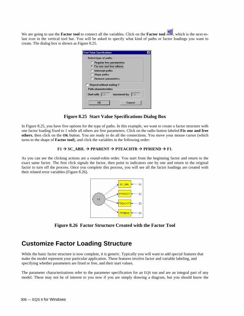
306 — EQS 6 for Windows
We are going to use the Factor tool to connect all the variables. Click on the Factor tool , which is the next-to-last icon in the vertical tool bar. You will be asked to specify what kind of paths or factor loadings you want to create. The dialog box is shown as Figure 8.25.
Figure 8.25 Start Value Specifications Dialog Box In Figure 8.25, you have five options for the type of paths. In this example, we want to create a factor structure with one factor loading fixed to 1 while all others are free parameters. Click on the radio button labeled Fix one and free others, then click on the OK button. You are ready to do all the connections. You move your mouse cursor (which turns to the shape of Factor tool), and click the variables in the following order:
F1 SC_ABIL PPARENT PTEACHTR PFRIEND F1.
As you can see the clicking actions are a round-robin order. You start from the beginning factor and return to the exact same factor. The first click signals the factor, then point to indicators one by one and return to the original factor to turn off the process. Once you complete this process, you will see all the factor loadings are created with their related error variables (Figure 8.26).
Figure 8.26 Factor Structure Created with the Factor Tool
Customize Factor Loading Structure While the basic factor structure is now complete, it is generic. Typically you will want to add special features that make the model represent your particular application. These features involve factor and variable labeling, and specifying whether parameters are fixed or free, and their start values.
The parameter characterizations refer to the parameter specification for an EQS run and are an integral part of any model. These may not be of interest to you now if you are simply drawing a diagram, but you should know the
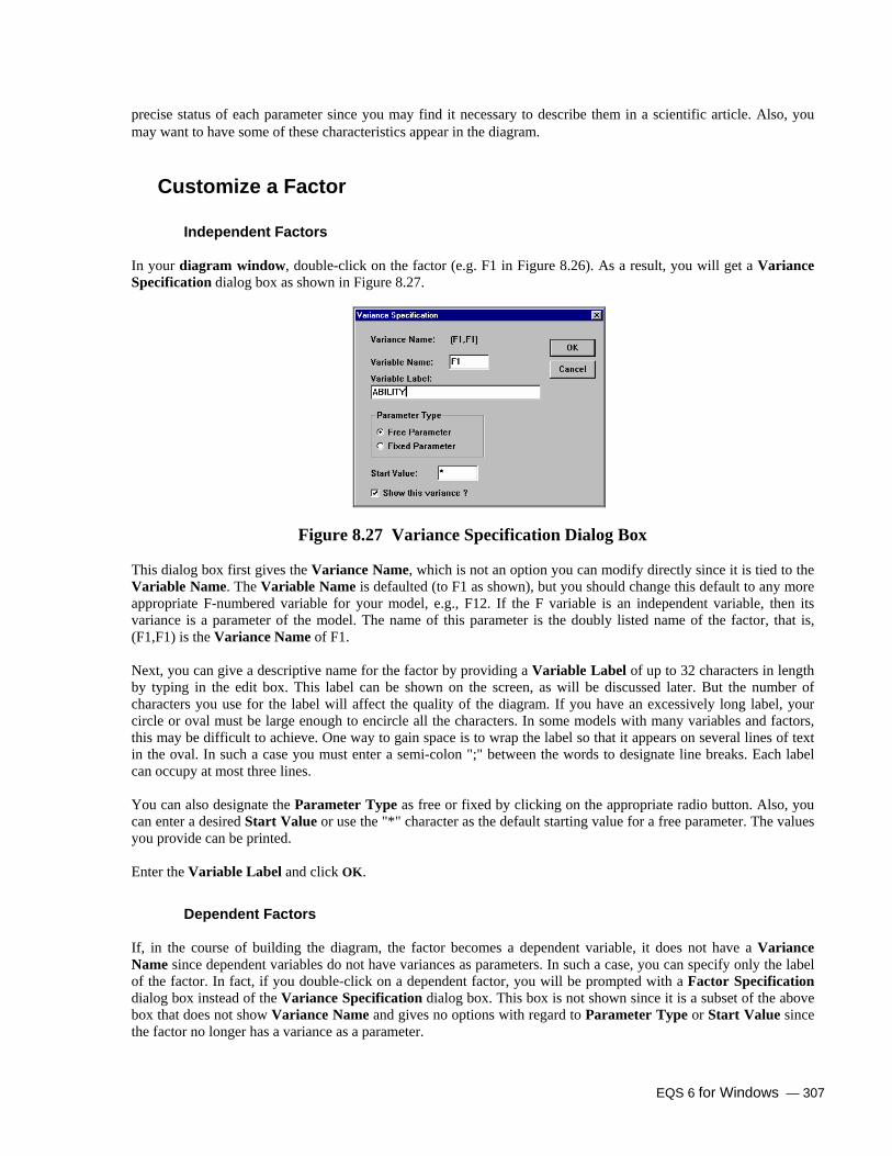
EQS 6 for Windows — 307
precise status of each parameter since you may find it necessary to describe them in a scientific article. Also, you may want to have some of these characteristics appear in the diagram.
Customize a Factor
Independent Factors
In your diagram window, double-click on the factor (e.g. F1 in Figure 8.26). As a result, you will get a Variance Specification dialog box as shown in Figure 8.27.
Figure 8.27 Variance Specification Dialog Box This dialog box first gives the Variance Name, which is not an option you can modify directly since it is tied to the Variable Name. The Variable Name is defaulted (to F1 as shown), but you should change this default to any more appropriate F-numbered variable for your model, e.g., F12. If the F variable is an independent variable, then its variance is a parameter of the model. The name of this parameter is the doubly listed name of the factor, that is, (F1,F1) is the Variance Name of F1. Next, you can give a descriptive name for the factor by providing a Variable Label of up to 32 characters in length by typing in the edit box. This label can be shown on the screen, as will be discussed later. But the number of characters you use for the label will affect the quality of the diagram. If you have an excessively long label, your circle or oval must be large enough to encircle all the characters. In some models with many variables and factors, this may be difficult to achieve. One way to gain space is to wrap the label so that it appears on several lines of text in the oval. In such a case you must enter a semi-colon ";" between the words to designate line breaks. Each label can occupy at most three lines. You can also designate the Parameter Type as free or fixed by clicking on the appropriate radio button. Also, you can enter a desired Start Value or use the "*" character as the default starting value for a free parameter. The values you provide can be printed. Enter the Variable Label and click OK.
Dependent Factors If, in the course of building the diagram, the factor becomes a dependent variable, it does not have a Variance Name since dependent variables do not have variances as parameters. In such a case, you can specify only the label of the factor. In fact, if you double-click on a dependent factor, you will be prompted with a Factor Specification dialog box instead of the Variance Specification dialog box. This box is not shown since it is a subset of the above box that does not show Variance Name and gives no options with regard to Parameter Type or Start Value since the factor no longer has a variance as a parameter.

308 — EQS 6 for Windows
Customize a Measured Variable Typically you will want to label the measured variables using more appropriate names. In the diagram window, double-click a V variable you are interested in (let’s use the variable labeled SC_ABIL as an example). You will obtain the Measured Variable Specification dialog box shown in Figure 8.28.
Figure 8.28 Measured Variable Specification Dialog Box By default, the dialog box has V1 entered in the Variable Name field. You can change V1 to the correct variable name if this variable is not the first variable in your data file. You can also enter a character string in the edit box labeled Variable Label to give the variable a meaningful acronym. As for the label in Figure 8.27, the string cannot exceed 32 characters, and you may wrap the label on two or three lines. In a factor model, measured variables are dependent variables. Since this variable is a dependent variable, its variance is not a parameter of the model and hence there is no need to specify its start value or whether it is a fixed or free parameter.
Independent Variables If this measured variable were an independent variable, you would see Variance Specification dialog box (Figure 8.27) instead of the Measured Variable Specification box. As was shown in Figure 8.27, this also gives you options with regard to Parameter Type and Start Value since an independent variable has a variance as a parameter. See the description of Figure 8.27 for details on these options.
Customize a Path or a Factor Loading You can also customize a path or a factor loading by doubleclicking on the path in the diagram window to get a Parameter Specification dialog box (Figure 8.29, below). Precision is very important when clicking on the path. You should click right at the edge of the square or circle in the location where you want the path to originate. You must click on the line, or very close to it. Otherwise, the path object will not be picked or the wrong object could be picked. You will easily achieve precision with some practice.
Figure 8.29 Parameter Specification Dialog Box
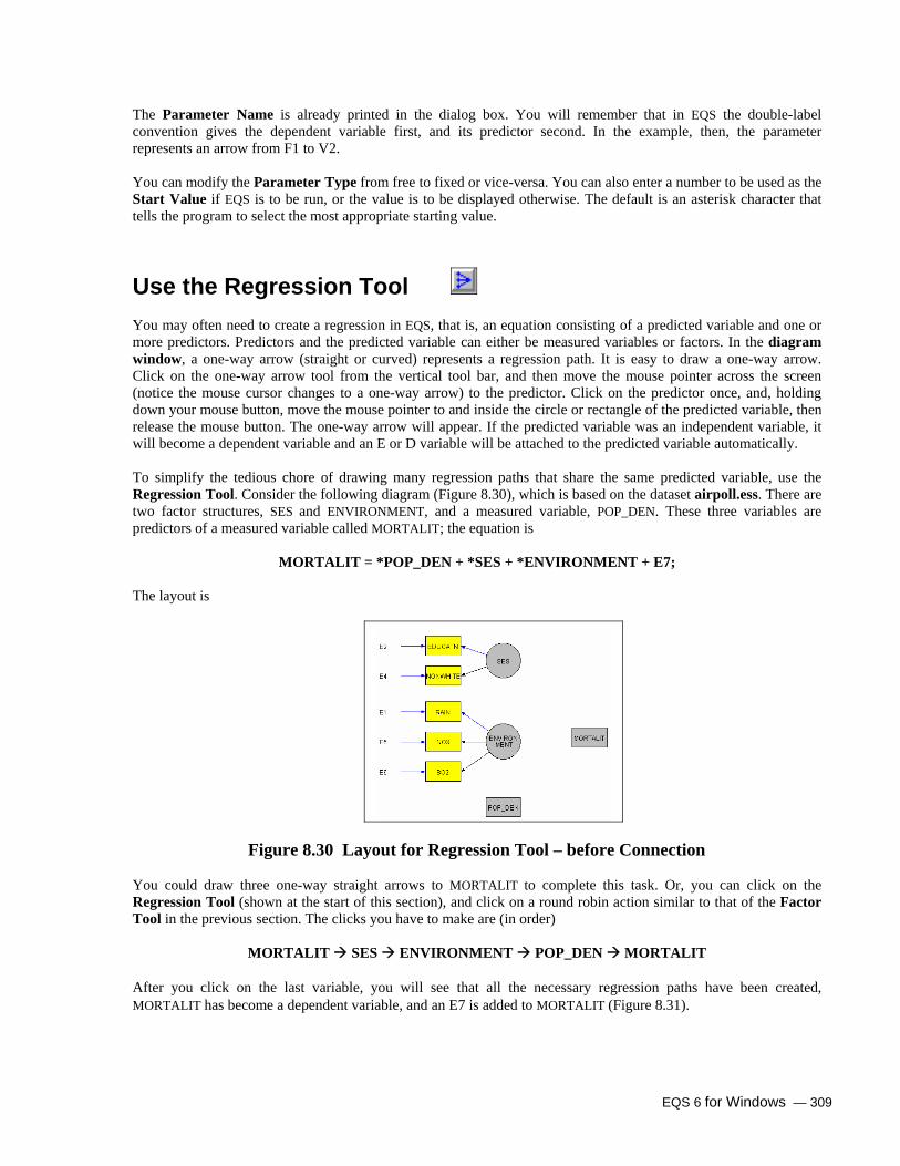
EQS 6 for Windows — 309
The Parameter Name is already printed in the dialog box. You will remember that in EQS the double-label convention gives the dependent variable first, and its predictor second. In the example, then, the parameter represents an arrow from F1 to V2. You can modify the Parameter Type from free to fixed or vice-versa. You can also enter a number to be used as the Start Value if EQS is to be run, or the value is to be displayed otherwise. The default is an asterisk character that tells the program to select the most appropriate starting value.
Use the Regression Tool You may often need to create a regression in EQS, that is, an equation consisting of a predicted variable and one or more predictors. Predictors and the predicted variable can either be measured variables or factors. In the diagram window, a one-way arrow (straight or curved) represents a regression path. It is easy to draw a one-way arrow. Click on the one-way arrow tool from the vertical tool bar, and then move the mouse pointer across the screen (notice the mouse cursor changes to a one-way arrow) to the predictor. Click on the predictor once, and, holding down your mouse button, move the mouse pointer to and inside the circle or rectangle of the predicted variable, then release the mouse button. The one-way arrow will appear. If the predicted variable was an independent variable, it will become a dependent variable and an E or D variable will be attached to the predicted variable automatically. To simplify the tedious chore of drawing many regression paths that share the same predicted variable, use the Regression Tool. Consider the following diagram (Figure 8.30), which is based on the dataset airpoll.ess. There are two factor structures, SES and ENVIRONMENT, and a measured variable, POP_DEN. These three variables are predictors of a measured variable called MORTALIT; the equation is
MORTALIT = *POP_DEN + *SES + *ENVIRONMENT + E7; The layout is
Figure 8.30 Layout for Regression Tool – before Connection You could draw three one-way straight arrows to MORTALIT to complete this task. Or, you can click on the Regression Tool (shown at the start of this section), and click on a round robin action similar to that of the Factor Tool in the previous section. The clicks you have to make are (in order)
MORTALIT SES ENVIRONMENT POP_DEN MORTALIT After you click on the last variable, you will see that all the necessary regression paths have been created, MORTALIT has become a dependent variable, and an E7 is added to MORTALIT (Figure 8.31).

310 — EQS 6 for Windows
Figure 8.31 Layout for Regression Tool – after Connection
Use the Covariate Tool One common practice in a Confirmatory Factor Analysis (CFA) model is to inter-correlate all factors. Each correlation between two factors means connecting them with a two-way arrow in the Diagrammer. When the number of factors gets larger, you need to draw lots of two-way arrows. To make this tedious task easy, use the Covariate Tool. Figure 8.32 shows a twelve-variable four-factor model. You could draw six two-way arrows to connect all the factors. Instead, we can use the Covariate Tool to connect all of them with just a few clicks. Like Factor tool and Regression, the Covariate tool uses round-robin clicking to form all possible correlations.
Figure 8.32 Uncorrelated Four-Factor CFA Model Click on the Covariate tool icon (shown at the top of this section). Then move your mouse to the diagram window and do the following clicks:
F1 F2 F3 F4 F1 You choose a starting factor, then click sequentially on the factors you want to include, then return to the original factor. All the factors you click must be independent variables; otherwise your clicks will have no effect. Figure 8.33 shows all possible factor correlations. Covariate tool can apply to any independent variables whether they are factors, measured variables, error variables, and/or disturbances.

EQS 6 for Windows — 311
Figure 8.33 Cross-Correlated CFA Model
Align Variables After all the objects are drawn, you may want to align the lines, circles, and rectangles so that they look good on the screen, and hence will look good on paper when the diagram is printed. The Diagrammer provides several ways to align objects, permitting you to create a customized and beautiful layout of your diagram.
Note: To align several diagram objects, you must highlight all the objects to be aligned by dragging a
rubber rectangle to encircle them.
That is, click your mouse button above and to the left of the objects to be aligned. Holding it down, drag it down and to the right until the rubber rectangle encloses all the objects. Once the objects are selected, click on the Layout menu from the main menu bar, and select an alignment scheme. The alignment schemes are discussed in detail in Chapter 9. Among them, you probably will use the tools Align Vertical and Align Horizontal most frequently. The two sets of rectangles shown below illustrate the effect. On the left you see three variables that are not well aligned. After vertical alignment is applied, they line up vertically in a straight line.
Before Vertical Alignment After Vertical Alignment
Create One Group Structure from Several Objects In the above example, each V variable had been defined as a separate object. After aligning all of these variables, they remain as individual objects. If, for any reason, one of the Vs gets moved, the alignment will not be maintained,

312 — EQS 6 for Windows
and you might have to realign the objects again. In order to keep this problem from occurring, the Diagrammer allows you to group several objects into a single structure. After grouping, you can move the entire structure as if it is a single object. The interrelations among the objects that exist at the time you group them are then maintained. Thus whenever you are satisfied with a particular set of objects, it is a good idea to link them into one group object.
Note: To group a set of variables and linkages as an object, you must encircle all the objects in a rubber
rectangle. Then, pull down the LAYOUT menu and select the GROUP menu item.
Thereafter, the highlighted individual object frames will disappear and be replaced by the group frame. Once a set of objects becomes a single group, you can move this new object anywhere in the diagram window, and its components will move as a unit. On the other hand, you cannot edit or customize a group object. If you want to modify any component of a group object, e.g., the label of a factor, you will have to first break the structure, make the modification, and finally re-group the objects.
Draw a Measured Variable There are times when you need to add a new V variable to your diagram. For example, you may want to add a new independent measured variable to your model. In such a situation, choose the V icon from the left-hand buttons on the tool bar in the diagram window, and then click on the location in the window where this variable should be placed. Once there, you may need to add the relevant connections of this variable to other variables. For example, the variable may be an indicator of a factor. If the added measured variable can be logically thought of as part of a particular structure, for example as part of a one-factor model with its indicators, it is a good idea to regroup the objects by including the new variable in that group.
Do not Draw Errors and Disturbances As we have suggested in the drawing rules, you don't have to draw E and D variables. The diagram has internal rules that cover all of the typical uses of such variables, and will generate these residual variables automatically. As an example, when a V variable is connected to an F variable by a one-way path of the sort F⎯>V, it is clear that the V variable must become a dependent variable. Consequently the diagram will generate an E variable automatically that will point to the V. Similarly, when an F variable is predicted by another F or a V variable, it becomes a dependent variable and its residual D variable will be generated automatically. These internal rules permit the diagram to make your model accurate as well as complete.
Note: On the other hand, there are times when generated E and D variables are not essential to your
model. You will have to take responsibility for deleting them from the diagram.
Connect All Elements After you have specified all the diagram elements such as factor structures and independent manifest variables, you are ready to connect them. The principal rule for connecting variables is to use a one-way arrow as a regression predictor, and a curved two-way arrow as a correlation or covariance. We shall use two examples to illustrate how arrows are drawn, one a straight arrow and the other a curved arrow. These two arrows require somewhat different strategies of connection.

EQS 6 for Windows — 313
Draw a straight arrow In this example we want to create a two-factor structural equation model. This is done in sequence. First, we use the factor structure object to create F1 with its indicators (a three-variable factor structure), and then repeat the process to create F2 with its indicators. At this point, the two factors F1 and F2 are not connected. In a confirmatory factor model, the factors must be connected by a two-way arrow to represent their correlation. In a standard regression model, F2 is predicted from F1, so we need to use a straight arrow to make the connection. This means that we create a simple regression where F1 is the predictor variable and F2 is the dependent variable. Here are the steps to draw the arrow.
Step 1. Click once on the straight one-way arrow in the tool bar. Step 2. Move the mouse pointer into the Diagram window. It becomes a crosshair (like a +). Place the
crosshair inside F1. Please note that you have to place the mouse pointer within the circle that defines F1.
Step 3. Hold the mouse pointer down and drag the mouse pointer to F2. Notice that when you are
dragging, the mouse cursor will take on a pencil shape. Release the mouse pointer when the pencil tip is located within the border of F2.
Step 4. Once the mouse pointer is released, a straight line will be drawn that connects F1 and F2, with the
arrowhead aiming at F2. The residual D2 will be attached to F2 automatically. If the alignment between D2 and F2 is not what you want, you can apply an alignment rule to correct it. Figure 8.34 is the result of this sequence of actions.
Figure 8.34 Two-Factor Structural Equation Model

314 — EQS 6 for Windows
Draw a curved arrow This time let us create a two-factor confirmatory factor model, in which the factors are correlated. Create the two unconnected factors with their indicators as in the previous example. We want to use a curved arrow to connect the two independent variables F1 and F2.
Step 1. Click once on the curved two-way arrow in the tool bar. Step 2. Move the mouse pointer to the Diagram window. The mouse cursor will become a crosshair
when it moves into the Diagram window. Put the mouse pointer within the circle of F1, and click and hold the mouse button. (Suggestion to the left-handers: you can start drawing from the upper left corner of F2. The effect will be identical when drawing a two-way arrow.)
Step 3. As you hold down the mouse button, drag the mouse pointer. It will become a pencil. Then,
release the mouse button when the mouse pointer is inside F2. You have to make sure that the mouse pointer is within F2's circle before it is released.
Step 4. Once the mouse button is released, a curved two-way arrow will attach to the left hand side of the
two factors. The left side of Figure 8.35 shows an example of such an arrow. By default, a curved arrow (one-way or two-way) will be shaped like the letter C if the two variables it connects are vertically aligned, or shaped like an upside-down U if the two variables are horizontally aligned.
Note: If you want the curved line to be shaped like a backwards C, or shaped like a U, you must hold down the SHIFT key when drawing the line. The right side of Figure 8.35 shows the effect.
Figure 8.35 Two-Factor Confirmatory Factor Analysis Model

EQS 6 for Windows — 315
Run EQS from a Diagram You would probably like to know how to run EQS after going through all these steps to draw a model. Let’s use the example illustrated earlier this chapter titled Build a Confirmatory Factor Analytic Model. This example uses a dataset manul7.ess with the model shown on the left side of Figure 8.35.
Build an EQS Model File After you have opened the data file and drawn the diagram, you are ready to build the EQS model. First, click on Build_EQS from the main menu. You can see, in the drop-down menu, that there are many items, but only two are active. The active options are black, while the inactive options are grayed out. This choice of only two options indicates that you should start with the item on top of the menu, Title/Specifications, to build the EQS model. You will be asked to save the diagram before the Title/Specifications dialog box appears. When drawing an EQS model using the Factor Model template, EQS 6 uses FACMOD.EDS as the default diagram file name. You want to save this diagram as MANUL7.EDS since this name coincides with your data file name. By selecting this option, you will see a new dialog box. This dialog box called EQS Model Specifications will appear as shown in Figure 8.36. This box has the information that is needed in the /SPECIFICATIONS section of the EQS program. By default, it automatically has most of the information you need to specify a model. Some of the default information is from the *.ess file (here, manul7.ess), and some reflects choices typically made in structural modeling. The file name, number of variables, number of cases, method of analysis, and type of input data (raw data, covariance matrix, etc.) have been set to defaults.
Figure 8.36 EQS Model Specifications Dialog Box

316 — EQS 6 for Windows
EQS Model File Click the OK button to close the dialog box. You will see that the EQS command language is built line by line and is written onto the background window. The file that is created is called manul7.eqx by default. The following shows part of the model file that is created. You are now ready to run EQS.
/TITLE EQS model created by EQS 6 for Windows /SPECIFICATIONS DATA='c:\EQS61\Examples\Manul7.ess'; VARIABLES=6; CASES=50; GROUPS=1; OUT=HTML; METHODS=ML; MATRIX=RAW; ANALYSIS=COVARIANCE; /LABELS V1=V1; V2=V2; V3=V3; V4=V4; V5=V5; V6=V6; /EQUATIONS V1 = + 1F1 + 1E1; V2 = + *F1 + 1E2; V3 = + *F1 + 1E3; V4 = + 1F2 + 1E4; V5 = + *F2 + 1E5; V6 = + *F2 + 1E6; /VARIANCES F1 = *; F2 = *; E1 = *; E2 = *; E3 = *; E4 = *; E5 = *; E6 = *; /COVARIANCES F2 , F1 = *; /PRINT EIS; FIT=ALL; TABLE=EQUATION; /END
If you need to add any options to the model, you must go to the Build_EQS menu and select the appropriate menu for your options. When a new command function is activated, the EQX file window will be re-drawn to update the changes. Notice that this window is not editable. Thus, all the changes to an EQS model must be done in relevant dialog boxes.
Run EQS To run EQS, go back to the Build_EQS menu and select Run EQS to run EQS. Before the program actually runs the EQS job, it displays a Save As dialog box as in Figure 8.7. You must save your EQS model file before running it. We have been working on the manul7.ess data, you have saved the diagram file as manul7.eds, and thus the default file name for the EQS model is manul7.eqx. In naming your file, set the file name to coincide with your data file name so that you will more easily remember what the job actually is.

EQS 6 for Windows — 317
The output from the run will have your specified file name, with the *.out extension. So, work.eqx will yield work.out as the output file, and manul7.eqx will yield manul7.out, and mode1.eqx will yield model.out.
Examine the EQS Output File
When EQS model run is complete, the output is automatically fetched to the front window. If you choose to display a regular ASCII output, the output file will be displayed in a text editor. You can scroll up and down. You can even use the Find/Replace function to locate specific information. For details on viewing the output, see the section on Editing Other Types of Files in Chapter 3. The first part of the output will echo your input file, so that you can verify what job was actually run. Beyond that, the output file includes all the standard results from a structural modeling run. We do not describe this output any further, however, because it is fully documented in the EQS 6 Structural Equations Program Manual.
Examine EQS Output on the Diagram If you have created the EQS model using the diagram method, the parameter estimates will be brought to the diagram when the job is done. When building an EQS model file using Diagrammer, the program will insert an EIS command in the /PRINT section automatically. The EIS command will write all estimates to an external file called eqs_file_name.eis, where eqs_file_name is your EQS model file name. The Diagrammer can read those estimates later, after the EQS job is done. To review the parameter estimates from the diagram, choose the Window menu and select the diagram file name (i.e., manul7.eds). The diagram window will appear with some basic statistics displayed at the bottom. If you want to see the parameter estimates of each parameter, you must click the View menu and select Estimates and then Parameter estimates. The diagram window will be redrawn with parameter estimates embedded in the paths (Figure 8.37).
0.55
V1
V2
V3
F1--0.48
0.67
0.72
0.29
V4
V5
V6
F2--0.18
0.64
0.20
Figure X: EQS 6 manul7a.eds Chi Sq.=2.70 P=0.95 CFI=1.00 RMSEA=0.00
0.74
1.48
1.89
1.07
0.12

318 — EQS 6 for Windows
Figure 8.37 Path Diagram with Embedded Parameter Estimates
Modify Model and Run EQS Again You may decide to modify the model, e.g., to add another path. If you do this, you should modify the diagram in Diagrammer, and then go to Build_EQS and follow the usual sequence of steps.
Note: Do not make changes in the *.eqx file until your model has been respecified with Diagrammer.
The program uses the sequence Diagrammer Build_EQS Run EQS. If you change equations, variances, or covariances in Build_EQS rather than in Diagrammer, the diagram (*.eds file) and model files (*.eqx file) will not match, and the program will bomb. Of course, you can abandon your diagrams, and work only with *.eqx files. Very large models are often more cumbersome with Diagrammer than without it.

EQS 6 for Windows — 319
9. DIAGRAM CUSTOMIZATION We have discussed the principles of drawing and customizing a diagram in Chapter 8, Build EQS by Drawing a Diagram. This chapter provides more details on the options available for editing and laying out a diagram. The Edit and Layout menus in the Diagrammer menu bar can be used to improve the appearance of a diagram, especially its alignment and spacing. Each diagram element in the Diagrammer is an object. Objects include rectangles (for V, E, and D variables), circles (for F variables), one-way arrows, two-way arrows, and factor structures (a combination of objects).
Note: To manipulate these objects, you must first select (highlight) them. The edit and layout functions only apply to those selected objected.
Select Objects There are four ways to select objects.
Select a Single Object To select a single object simply click on the object. For rectangles and circles, click anywhere within the object. For arrows, click carefully on the straight or curved line. After you click on an object, it will be framed by a rectangle.
Select a Group of Contiguous Objects You can drag a rubber rectangle to encircle the target objects. You must enclose each object completely within the rectangle. Any partially-enclosed objects will not be selected. Thus, if you enclose only one object that is part of a group of objects, neither the group nor the individual object will be selected.
Select a Group of Non-Contiguous Objects You cannot drag a rubber rectangle to select non-contiguous objects because you would also select the unwanted objects among them. To select (e.g., two objects separated by a third object) hold down the <Shift> key while you select each object by clicking on it (see above).
Select All Objects of a Certain Type You can select all objects of a certain type, or all objects in the diagram, by clicking on Select Drawing Objects in the Edit menu. See Figure 9.1. When the draw window is empty, all the menu items are grayed out except Select Drawing Objects and Deselect All. After some objects are drawn and selected, some more options will be activated.

320 — EQS 6 for Windows
Edit Menu The Edit menu includes the following options:
Figure 9.1 Diagrammer Edit Menu
Undo Clicking on Undo will cancel the effect of the last operation. It is active only when that operation was a horizontal or vertical flip, a rotation, or anything from the Layout menu except Group and Break Group.
Cut The Cut option copies the selected objects into the Windows Clipboard and removes them from the draw window.
Procedure: • Select one or more objects from the draw window. • Click on Edit in the main menu. This activates the Edit menu. • Click on Cut from the Edit menu.
Copy
The Copy option copies the selected objects into the Clipboard but leaves them in the draw window. Procedure: • Select one or more objects from the draw window. • Click on Edit in the main menu. This activates the Edit menu. • Click on Copy from the Edit menu.

EQS 6 for Windows — 321
Paste
The Paste option copies the contents of the Clipboard back into the draw window, at the position of the cursor. It is active only when the Clipboard has something in it, as the result of a Cut or Copy.
Procedure: • Click on Edit in the main menu. This activates the Edit menu. • Click on Paste from the Edit menu.
Clear
The Clear option removes selected objects from the draw window. Unlike the Cut option, it does not copy the selected objects into the Clipboard.
Procedure: • Select one or more objects from the draw window. • Click on Edit in the main menu. This activates the Edit menu. • Click on Clear from the Edit menu.
Import
The Import option allows you to import parameter values from a *.ETS file created by a previous run. Clicking on this option will open a dialog box, so that you can choose which file to import.
Select Drawing Objects
This option allows you to select all objects of a certain type, or all objects in the diagram. After clicking on this option, the menu on the right side of Figure 9.1 will let you choose which objects to select.
One example of using the Select All Diagram Objects option is to select all the objects and make them a single group. See the Group option later in this chapter. Once you have made your diagram a single object, you can apply layout commands to make the diagram look nicer before it is printed. See layout options later this chapter.
Procedure: • Click on Edit in the main menu. This activates the Edit menu. • Click on Select Drawing Objects so that your screen looks like Figure 9.1. • Click on Select All from the menu on the right.
Deselect All
The Deselect All option is the counterpart of the Select All option. It deselects all the objects that have been selected. If no object is selected from the draw window, this option has no effect.
Procedure: • Click on Edit in the main menu. This activates the Edit menu. • Click on Deselect All item from the Edit menu.
Horizontal Flip
The Horizontal Flip option allows you to replace a group object by its horizontal mirror image. This is an easy way to create such an effect without redrawing all the objects in the group. It does not make sense to apply Horizontal Flip to an individual object such as a variable because its appearance will not change. When applied to a one-way arrow, it may result in an unpredictable outcome. Figure 9.2 is an example of a group object before and after the

322 — EQS 6 for Windows
horizontal flip. Note that labels are preserved, e.g. V1 is still V1, not 1V. Flipping twice returns the object to its original form, i.e., flipping the object on the left results in the object on the right, and vice-versa.
Figure 9.2 Layout before and after Horizontal Flip Procedure: • Select the group object to be flipped from the draw window. • Click on Edit in the main menu. This activates the Edit menu. • Click on Horizontal Flip from the Edit menu.
Vertical Flip
This option is analogous to Horizontal Flip; it flips an object vertically. Like the Horizontal Flip option, it should be used to flip a group object, it preserves labels, and flipping twice restores the object to its original form. Figure 9.3 is an example of a group object before and after the vertical flip.
Figure 9.3 Layout before and after Vertical Flip
Procedure: • Select the group object to be flipped from the draw window. • Click on Edit in the main menu. This activates the Edit menu. • Click on Vertical Flip from the Edit menu.
Rotate
This option gives you another way to change the orientation of an object. Each Rotate will turn an object 90 degree clockwise. Like the Flip options above, it should be applied to a group object, and it preserves labels. Applying Rotate four times will restore an object to its original form. Figure 9.4 is an example of the effect of Rotate.

EQS 6 for Windows — 323
Figure 9.4 Layout before and after Rotate (Left and Right, Respectively)
Procedure: • Select the group object to be rotated from the draw window. • Click on Edit in the main menu. This activates the Edit menu. • Click on Rotate from the Edit menu.
Curve1 and Curve2
These options are inactive in this version.
Preference
This option allows you to set preferences for EQS model runs. See Chapter 10.
Layout Menu
The commands in the Edit menu allow you to manipulate or change the orientation of an object. The Layout menu helps you to organize and beautify your diagram. In this section you will learn:
• How to group several objects into one single object • How to break a group object into its components • How to align objects • How to center your diagram so that it looks nice on the printout • How to equalize the spacing between objects

324 — EQS 6 for Windows
The Layout menu includes the following options:
Figure 9.5 The Layout Menu
Group
This is one of the most important editing commands in the Diagrammer. It transforms several objects into one single group object. Once these objects are grouped, the relative position of each group member will remain constant. You can manipulate this group object without worrying about its members. For example, you can cut, paste, flip, or rotate a group object as if you are dealing with an individual drawing element.
To find out whether an object is part of a group, click on it. If the bounding rectangle (i.e., a rectangle surrounding the object, marked by tiny squares) covers several neighboring objects, then the object you selected belongs to the group marked by the bounding rectangle. If the bounding rectangle covers no other objects, the object you selected does not belong to a group. See Figure 9.6, below.
Use the following procedure to create a group. Procedure:
8. Select the objects to be grouped from the draw window. See Select Objects at the start of this chapter. Remember that only one group will be created, no matter how many objects are selected.
9. Click on Layout in the main menu. This activates the Layout menu. 10. Click on Group from the Layout menu. The individual bounding rectangles will disappear
and be replaced by a bounding rectangle that covers the entire group. Figure 9.6 shows an example of objects before and after grouping.
Before Group After Group
Figure 9.6 Example of Grouping

EQS 6 for Windows — 325
Break Group
The Break Group option is the opposite of the group option. It breaks a group object into individual drawing elements such as rectangles, one-way arrows, and factors. This option is essential when you want to modify the information on a drawing element that is the member of a group object. To customize a group member, you have to break the group first.
Procedure: • Select a group object from the draw window. • Click on Layout in the main menu. This activates the Layout menu. • Click on Break Group from the Layout menu.
Vertical Alignment
After positioning all your diagram elements, you many notice that alignment, centering, and spacing of objects are somewhat uneven. While you could try to make the diagram look nicer by moving all the objects by hand, it is much easier to use the Layout menu options. The alignment and spacing commands apply only when you have selected multiple objects. Commands in the Layout menu will have effect if only one object is selected. We will illustrate vertical alignment in this section and horizontal alignment in the next section.
There are four ways to align your objects vertically. You can align the selected objects to the left, to the right, to the center, or to the center of the page.
Note: Before aligning the objects, they must be in a rough vertical line. If not, the results of the
alignment will be bad.
Align Left
This option will align the selected objects to the leftmost object selected. Procedure: • Select two or more objects. • Click on Layout in the main menu. This activates the Layout menu. • Click on Align Left from the Layout menu.
Align Right
This option will align the selected objects to the rightmost object selected. Procedure: • Select two or more objects. • Click on Layout in the main menu. This activates the Layout menu. • Click on Align Right from the Layout menu.
Align Vertical
This option will align the selected objects so that they are above or below a point halfway between the leftmost and rightmost objects selected. Procedure: • Select two or more objects. • Click on Layout in the main menu. This activates the Layout menu. • Click on Align Vertical from the Layout menu.
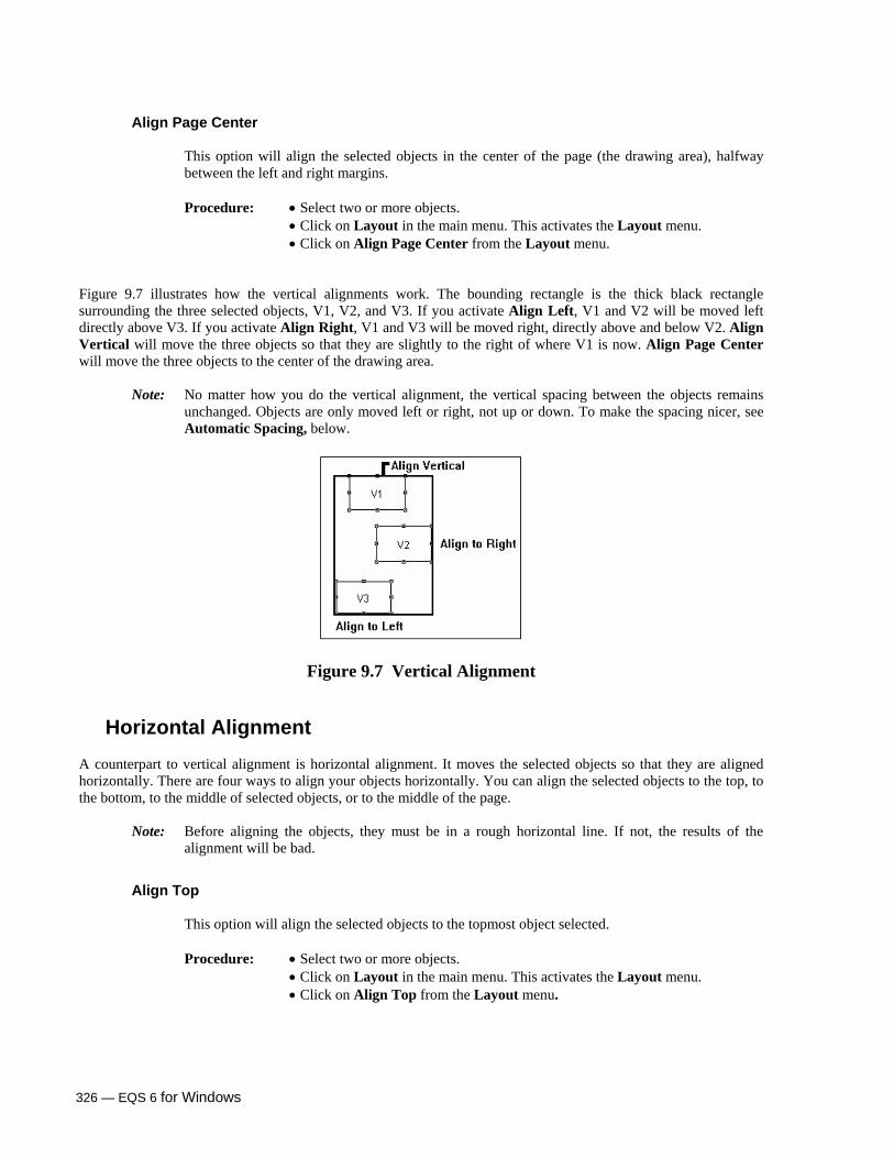
326 — EQS 6 for Windows
Align Page Center
This option will align the selected objects in the center of the page (the drawing area), halfway between the left and right margins. Procedure: • Select two or more objects. • Click on Layout in the main menu. This activates the Layout menu. • Click on Align Page Center from the Layout menu.
Figure 9.7 illustrates how the vertical alignments work. The bounding rectangle is the thick black rectangle surrounding the three selected objects, V1, V2, and V3. If you activate Align Left, V1 and V2 will be moved left directly above V3. If you activate Align Right, V1 and V3 will be moved right, directly above and below V2. Align Vertical will move the three objects so that they are slightly to the right of where V1 is now. Align Page Center will move the three objects to the center of the drawing area.
Note: No matter how you do the vertical alignment, the vertical spacing between the objects remains unchanged. Objects are only moved left or right, not up or down. To make the spacing nicer, see Automatic Spacing, below.
Figure 9.7 Vertical Alignment
Horizontal Alignment
A counterpart to vertical alignment is horizontal alignment. It moves the selected objects so that they are aligned horizontally. There are four ways to align your objects horizontally. You can align the selected objects to the top, to the bottom, to the middle of selected objects, or to the middle of the page.
Note: Before aligning the objects, they must be in a rough horizontal line. If not, the results of the
alignment will be bad.
Align Top
This option will align the selected objects to the topmost object selected. Procedure: • Select two or more objects. • Click on Layout in the main menu. This activates the Layout menu. • Click on Align Top from the Layout menu.

EQS 6 for Windows — 327
Align Bottom
This option will align the selected objects to the bottommost object selected. Procedure: • Select two or more objects. • Click on Layout in the main menu. This activates the Layout menu. • Click on Align Bottom from the Layout menu.
Align Horizontal
This option will align the selected objects so that they are to the right or left of a point halfway between the topmost and bottommost objects selected. Procedure: • Select two or more objects. • Click on Layout in the main menu. This activates the Layout menu. • Click on Align Horizontal from the Layout menu.
Align Page Middle
This option will align the selected objects in the middle of the page (the drawing area), halfway between the top and bottom margins. Procedure: • Select two or more objects. • Click on Layout in the main menu. This activates the Layout menu. • Click on Align Page Middle from the Layout menu.
Figure 9.8 illustrates how the horizontal alignments work. The bounding rectangle is the thick black rectangle surrounding the three selected objects (V1, V2, and V3). If you activate Align Top, V1 and V3 will move up so that they are even with V2. If you activate Align Bottom, V1 and V2 will move down so that they are even with V3. Align Horizontal will align the three objects in the middle between the top of V2 and the bottom of V3. Align Page Middle will move the three objects to the middle of the drawing area, halfway between the top and bottom.
Note: No matter how you do the horizontal alignment, the horizontal spacing between the objects
remains unchanged. Objects are only moved up or down, not left or right. To make the spacing nicer, see Automatic Spacing, below.
Align Top
Align Horizontal
Align Bottom
Figure 9.8 Horizontal Alignment

328 — EQS 6 for Windows
Automatic Spacing
In the previous two sections, we have shown how to align the drawing objects both vertically and horizontally. This alignment, however, does not change the spacing between objects. Evenly distributed objects will enhance the beauty of your diagram, but this is difficult to achieve by using your hands and eyes. Thus, we have provided two additional tools to achieve this objective. They are Even Horizontal Spacing and Even Vertical Spacing. These options allow you to modify the horizontal or vertical distances between objects without dragging the objects to new positions.
Even Horizontal Spacing
This option calculates the distance between the leftmost and rightmost object in the bounding rectangle, and evenly distributes the other objects between them. If you select only two objects, there will be no change. You must select at least three objects to apply this option. Figure 9.9 illustrates the Even Horizontal Spacing option. Notice that the objects move horizontally but not vertically.
Procedure: • Select three or more objects. • Click on Layout in the main menu. This activates the Layout menu. • Click on Even Hor Spacing from the Layout menu.
Before Even Horizontal Spacing
After Even Horizontal Spacing
Figure 9.9 Example of Even Horizontal Spacing
Even Vertical Spacing
The Even Vertical Spacing option is the counterpart to the Even Horizontal Spacing option. It also requires three or more objects to be effective. Figure 9.10 illustrates the Even Vertical Spacing option. Notice that the objects move vertically but not horizontally.
Procedure: • Select three or more objects. • Click on Layout in the main menu. This activates the Layout menu. • Click on Even Ver Spacing from the Layout menu.

EQS 6 for Windows — 329
Before Even Vertical Spacing After Even Vertical Spacing
Figure 9.10 Example of Even Vertical Spacing
A Word of Caution While it is usually desirable to have a beautiful diagram, remember that a less than perfect diagram will run the same model as a publication-quality diagram. It is more important to get the model right than to work with perfect diagrams, so spend your time accordingly. Of course, when you are ready to publish, or to give a public talk, an attractive diagram is a necessity.

330 — EQS 6 for Windows
10. PREFERENCES EQS 6 for Windows has many dialog boxes to specify various options. Although we have provided a set of options that we think are useful for your modeling purposes, we can’t possibly anticipate everyone’s interests. EQS Preferences is a series of tabbed dialog boxes where you can modify various EQS modeling settings so that these options become the defaults the next time you create an EQS model or run some general statistics. The changes in Preference will not alter an EQS model that has been specified. It, however, will affect the options for a new model that is about to be created. To access Preference, you must first open a file to bring up the Edit menu and then click on Preference… from the edit menu. The Preferences are organized into three sections:
1. General Preferences 2. EQS Model-Related Preferences 3. Basic Statistics Preferences
General Preferences The General Preferences include options that are commonly used by EQS throughout the program. Sample choices include: where the EQS model will be housed, where the temporary files go, the foreground and background color of a text editor, etc. See Figure 10.1 for details.
Figure 10.1 General Preferences
EQS Model-Related Preferences As the sophistication of EQS grows, there are more options to be specified. EQS 6 for Windows introduces many new tests and statistics; naturally, each one of them needs a check box or a radio button to be activated. Likewise, we need a few dialog boxes to house all these options in the Preference boxes. These are EQS specifications (Figure 10.2) for the /SPECIFICATION paragraph, EQS controls (Figure 10.3) for the /PRINT, /OUTPUT, and /TECHNICAL paragraphs, EQS Simulations (Figure 10.4) for the /SIMULATION paragraph, EQS Parameter tests (Figure 10.5) for

EQS 6 for Windows — 331
LM tests and Wald tests, EQS Diagram (Figure 10.6) for Diagrammer-related options, and EQS Save file (Figure 10.7) for the new /SAVE paragraph.
Figure 10.2 EQS Specifications Figure 10.3 EQS Controls
Figure 10.4 EQS Simulations Figure 10.5 EQS Parameter Tests
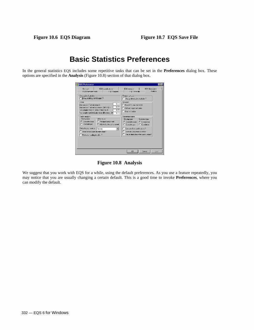
332 — EQS 6 for Windows
Figure 10.6 EQS Diagram Figure 10.7 EQS Save File
Basic Statistics Preferences In the general statistics EQS includes some repetitive tasks that can be set in the Preferences dialog box. These options are specified in the Analysis (Figure 10.8) section of that dialog box.
Figure 10.8 Analysis We suggest that you work with EQS for a while, using the default preferences. As you use a feature repeatedly, you may notice that you are usually changing a certain default. This is a good time to invoke Preferences, where you can modify the default.