equations of state - mfe experiments in p-24 plasma physics
TRANSCRIPT
Equations of State
Damian Swift
P-24 Plasma Physics
Los Alamos National Laboratory
[email protected] http://public.lanl.gov/dswift
1
Outline
• What is the equation of state and why should we care?
• Theoretical basis
• Complete and incomplete EOS
• Predicting the EOS
• Experimental measurements
• Corrections, limits, and other issues
2
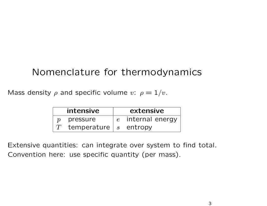
Nomenclature for thermodynamics
Mass density ρ and specific volume v: ρ = 1/v.
intensive extensive
p pressure e internal energyT temperature s entropy
Extensive quantities: can integrate over system to find total.
Convention here: use specific quantity (per mass).
3

What is the equation of state?
compression
block of matter
heat
What’s the pressure?
Material-dependent property, relating thermodynamic
potential and its natural parameters, e.g. de = Tds − pdv.EOS is the relation e(s, v) for a material.
Derivatives and other functions of EOS give other quantities:
p, T , sound speed c2, heat capacity cv, ...
Perfect gas EOS:
p = nkBT p = (γ − 1)ρe
4
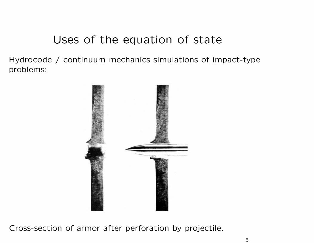
Uses of the equation of state
Hydrocode / continuum mechanics simulations of impact-type
problems:
Cross-section of armor after perforation by projectile.
5
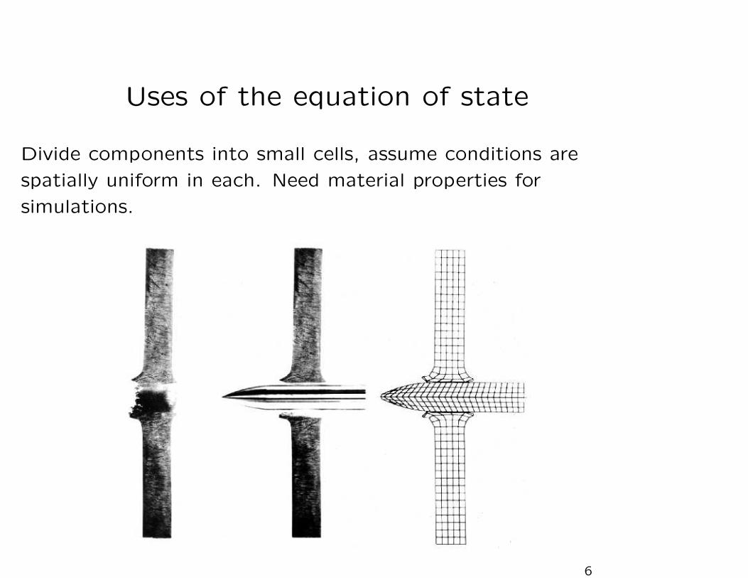
Uses of the equation of state
Divide components into small cells, assume conditions are
spatially uniform in each. Need material properties for
simulations.
6

Uses of the equation of state
Radiation-driven implosions, e.g. NIF hohlraum-driven fusion
capsule:
Source: J. Lindl, “Inertial confinement fusion,” Springer (1998).
7
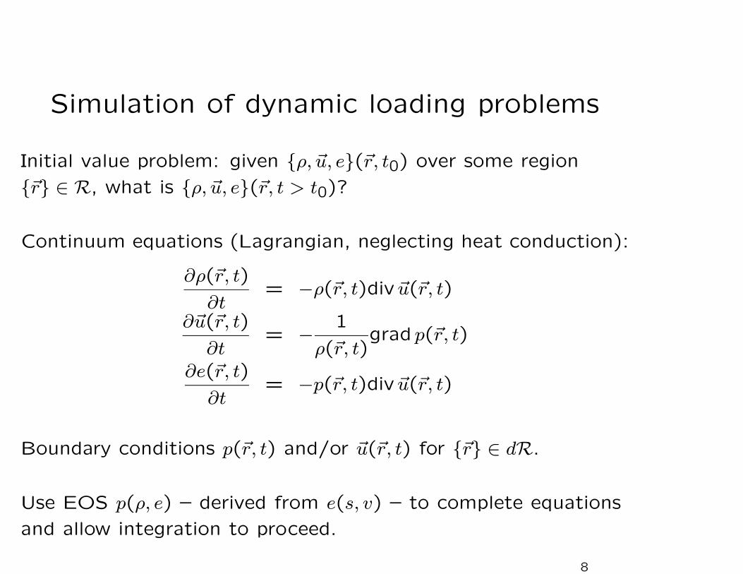
Simulation of dynamic loading problems
Initial value problem: given {ρ, ~u, e}(~r, t0) over some region
{~r} ∈ R, what is {ρ, ~u, e}(~r, t > t0)?
Continuum equations (Lagrangian, neglecting heat conduction):
∂ρ(~r, t)
∂t= −ρ(~r, t)div ~u(~r, t)
∂~u(~r, t)
∂t= − 1
ρ(~r, t)grad p(~r, t)
∂e(~r, t)
∂t= −p(~r, t)div ~u(~r, t)
Boundary conditions p(~r, t) and/or ~u(~r, t) for {~r} ∈ dR.
Use EOS p(ρ, e) – derived from e(s, v) – to complete equations
and allow integration to proceed.
8
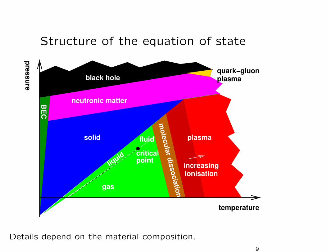
Structure of the equation of state
temperature
pre
ssu
re
black hole
neutronic matter
solid
gas
liquid
BE
C
quark−gluonplasma
pointcritical
fluid plasma
increasingionisation
mo
lecu
lar d
isso
cia
tion
Details depend on the material composition.
9

‘Moderate’ pressure and temperatureGeophysics, hypervelocity impact, terrestrial explosions, ICF, ...
−GPa (pspall) < p < PPa (Gbar); ∼ 10K < T < MeV; ps < t < Gyr
e.g. Cu:
0 1 2 3 4 5 6 7 8 910
ρ (g/cm3)
0 2000 4000 6000 8000 1000012000
T (K)
0123456789
e (MJ/kg)
solid
liquid
critical point
vapor
liquid/vapor
e(ρ, T ) = ecold(ρ) + eion-thermal(ρ, T ) + eelectron-thermal(ρ, T )
10

Cu phase diagram
SESAME #4:
0 1 2 3 4 5 6 7 8 910
ρ (g/cm3)
0 2000 4000 6000 8000 1000012000
T (K)
0123456789
e (MJ/kg)
solid
liquid
critical point
vapor
liquid/vapor
11

Energy, EOS, and phase diagram
Given e(ρ, T ) – for a given atomic arrangement – can construct
EOS using 2nd law of thermodynamics:
de = Tds − pdv ⇒ s(v, T ) = s(v,0) +∫ T
0
dT ′
T ′∂e(v, T ′)
∂T ′
from which calculate f(ρ, T ) = e(ρ, T ) − Ts(ρ, T ) ⇒ EOS for
this phase.
s(v,0): ‘configurational entropy’ – may vary between phases.
At any p, T , equilibrium phase has lowest Gibbs free energy
g = e − Ts + pv (natural parameters g(T, p) as dg = −sdT + vdp)
12

Phase diagram: Fe
Different crystal structures occur in the solid state:
0
5
10
15
20
25
30
35
40
45
50
0 500 1000 1500 2000 2500 3000 3500
pres
sure
(G
Pa)
temperature (K)
bccliquid
hcp fcc
bcc
13
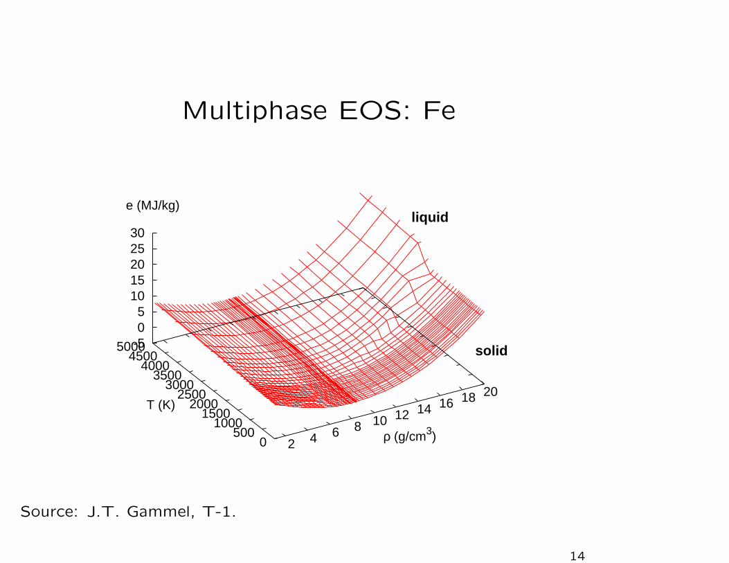
Multiphase EOS: Fe
2 4 6 8 10 12 14 16 18 20
ρ (g/cm3)0500
10001500
20002500
30003500
40004500
5000
T (K)
-505
1015202530
e (MJ/kg)
solid
liquid
Source: J.T. Gammel, T-1.
14
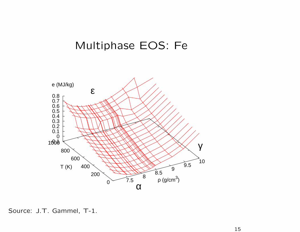
Multiphase EOS: Fe
7.58
8.59
9.510
ρ (g/cm3)0
200
400
600
800
1000
T (K)
-0.10
0.10.20.30.40.50.60.70.8
e (MJ/kg)ε
α
γ
Source: J.T. Gammel, T-1.
15

Thermodynamic completeness
Complete EOS: thermodynamic potential expressed in natural
parameters
e(s, v), f(T, v), g(T, p), h(s, p)
Can derive any thermodynamic parameter from a complete
EOS.
Continuum mechanics:
∂ρ/∂t = −ρdiv ~u, ∂~u/∂t = −(1/ρ)grad p, ∂e/∂t = −pdiv ~u
only require p(ρ, e).
Also: easiest to deduce p(ρ, e) from mechanical measurements.
Incomplete EOS: p(ρ, e) with no information about T .
‘SESAME’ EOS: e(ρ, T ) and p(ρ, T ): a complete EOS – but
may be inconsistent.
16
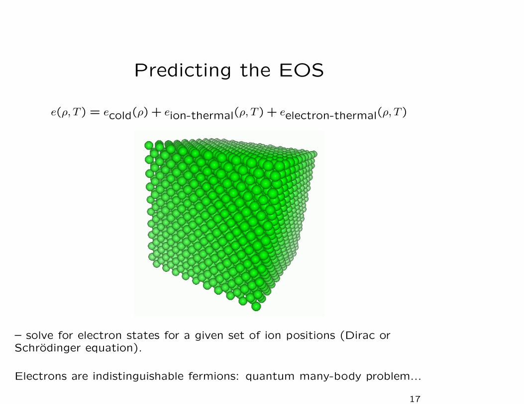
Predicting the EOS
e(ρ, T ) = ecold(ρ) + eion-thermal(ρ, T ) + eelectron-thermal(ρ, T )
– solve for electron states for a given set of ion positions (Dirac orSchrodinger equation).
Electrons are indistinguishable fermions: quantum many-body problem...
17

Quantum many-body problem
Ground state of collective wavefunction Ψ: HΨ = E0Ψ.
Numerical quantum mechanics: based on single-particle
wavefunctions {ψi}. Fermions: antisymmetric with respect to
particle exchange (Pauli exclusion principle), e.g. for 2-particle
wavefunctions Ψ(1,2) = −Ψ(2,1), can be satisfied if
Ψ(1,2) =1√2[ψ1(1)ψ2(2) − ψ2(1)ψ1(2)].
More generally,
Ψ(1,2, ...n) =∑
χε(χ)ψχ(i)(i) = detψi(j)
where ε is a permutation operator – ‘Slater determinant’
approach; in practice prohibitive in computer time.
Differences in the phase of the wavefunctions ⇒ correlation
effects: another complication.
18
Local density approximation
Assume can approximate exchange and correlation by
modifying the potential energy contribution in the Hamiltonian
to include functions of the local electron density
n(~r) =∑
i
ψ†i (~r)ψi(~r).
These functions are then calibrated against detailed exchange
and correlation calculations for simple systems e.g. uniform
electron gas.
Typical accuracy: a few percent in density at p = 0, T = 0.
19
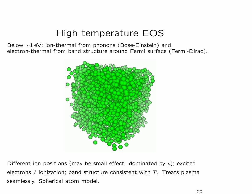
High temperature EOSBelow ∼1 eV: ion-thermal from phonons (Bose-Einstein) andelectron-thermal from band structure around Fermi surface (Fermi-Dirac).
Different ion positions (may be small effect: dominated by ρ); excited
electrons / ionization; band structure consistent with T . Treats plasma
seamlessly. Spherical atom model.
20
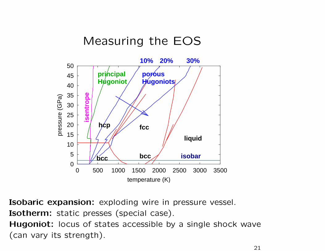
Measuring the EOS
0
5
10
15
20
25
30
35
40
45
50
0 500 1000 1500 2000 2500 3000 3500
pres
sure
(G
Pa)
temperature (K)
bcc
hcp fcc
bcc
liquid
isobar
isen
tro
pe
principalHugoniot
porousHugoniots
10% 20% 30%
Isobaric expansion: exploding wire in pressure vessel.
Isotherm: static presses (special case).
Hugoniot: locus of states accessible by a single shock wave
(can vary its strength).
21
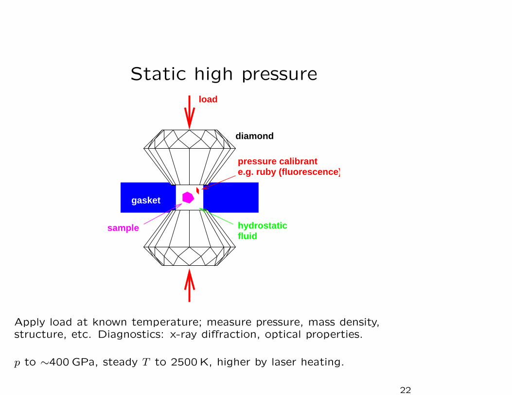
Static high pressure
gasket
diamond
load
pressure calibrante.g. ruby (fluorescence)
sample hydrostaticfluid
Apply load at known temperature; measure pressure, mass density,structure, etc. Diagnostics: x-ray diffraction, optical properties.
p to ∼400 GPa, steady T to 2500 K, higher by laser heating.
22
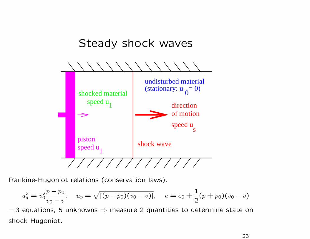
Steady shock waves
speed us
speed u1
speed u1
undisturbed material(stationary: u = 0)
0
directionof motion
shock wavepiston
shocked material
Rankine-Hugoniot relations (conservation laws):
u2s = v2
0
p − p0
v0 − v, up =
√
[(p − p0)(v0 − v)], e = e0 +1
2(p + p0)(v0 − v)
– 3 equations, 5 unknowns ⇒ measure 2 quantities to determine state on
shock Hugoniot.
23
Shock wave experiments
– ways to launch and measure a steady shock:
• Impact experiments (gas gun, powder gun, electromagnetic
flyer, explosively-driven flyer, laser flyer)
• Detonation-driven shock
• Radiation-driven shock (nuclear explosion, laser hohlraum)
• Laser ablation
Aspect ratio: thin samples to preserve 1D region in center.
24
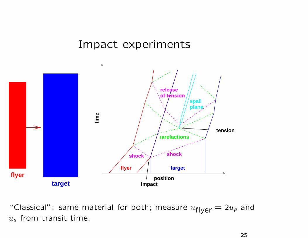
Impact experiments
targetflyer position
tim
e
targetflyer
shockshock
rarefactions
spallplane
impact
tension
releaseof tension
“Classical”: same material for both; measure uflyer = 2up and
us from transit time.
25
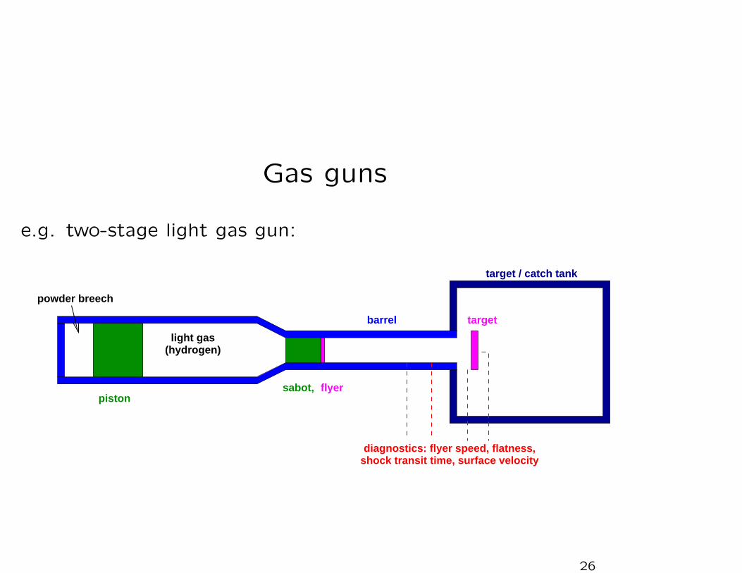
Gas guns
e.g. two-stage light gas gun:
barrel
target / catch tank
pistonsabot, flyer
target
light gas(hydrogen)
powder breech
diagnostics: flyer speed, flatness,shock transit time, surface velocity
26

Electromagnetic launcher
e.g. Z pulsed power machine:
and ablationaccelerate flyerfrom surface
electricalcurrent flow
performed in a recessin the panel wall
each experiment is
magnetic pressure
experiments on eachtwo or three
two or four panels;
27
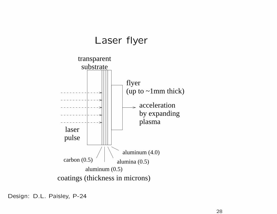
Laser flyer
transparentsubstrate
carbon (0.5)
aluminum (0.5)alumina (0.5)
aluminum (4.0)
coatings (thickness in microns)
laserpulse
flyer(up to ~1mm thick)
accelerationby expandingplasma
Design: D.L. Paisley, P-24
28

Laser flyer
spacer ring
(dried coffee)
working fluid
(molasses)
10 mm
substrate
(soda-lime glass)flyer
(copper)
assembly
(view through substrate)
29
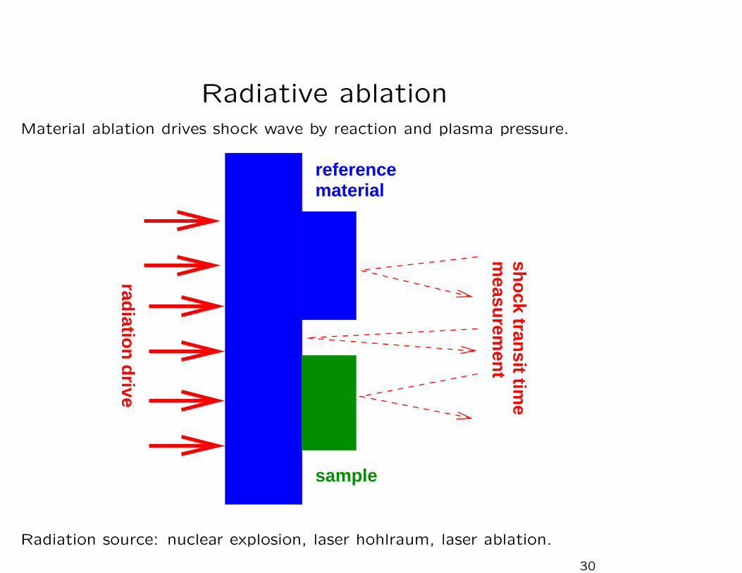
Radiative ablationMaterial ablation drives shock wave by reaction and plasma pressure.
referencematerial
sample
radiatio
n d
rive
sho
ck transit tim
em
easurem
ent
Radiation source: nuclear explosion, laser hohlraum, laser ablation.
30

Other shock diagnostics
surface velocimetry, radiography, transient x-ray diffraction
� � � � � � � � � � � � � � � �
� � � � � � � � � � � � � � � �
� � � � � � � � � � � � � � � �
� � � � � � � � � � � � � � � �
� � � � � � � � � � � � � � � �
� � � � � � � � � � � � � � � �
� � � � � � � � � � � � � � � �
� � � � � � � � � � � � � � � �
� � � � � � � � � � � � � � � �
� � � � � � � � � � � � � � � �
� � � � � � � � � � � � � � � �
� � � � � � � � � � � � � � � �
� � � � � � � � � � � � � � � �
� � � � � � � � � � � � � � � �
� � � � � � � � � � � � � � � �
� � � � � � � � � � � � � � � �
� � � � � � � � � � � � � � � �
� � � � � � � � � � � � � � � �
� � � � � � � � � � � � � � � �
� � � � � � � � � � � � � � � �
� � � � � � � � � � � � � � � �
� � � � � � � � � � � � � � � �
� � � � � � � � � � � � � � � �
� � � � � � � � � � � � � � � �
� � � � � � � � � � � � � � � �
� � � � � � � � � � � � � � � �
� � � � � � � � � � � � � � � �
� � � � � � � � � � � � � � � �
� � � � � � � � � � � � � � � �
� � � � � � � � � � � � � � � �
� � � � � � � � � � � � � � � �
� � � � � � � � � � � � � � � �
� � � � � � � � � � � �
� � � � � � � � � � � �
� � � � � � � � � � � �
� � � � � � � � � � � �
� � � � � � � � � � � �
� � � � � � � � � � � �
� � � � � � � � � � � �
� � � � � � � � � � � �
� � � � � � � � � � � �
� � � � � � � � � � � �
� � � � � � � � � � � �
� � � � � � � � � � � �
� � � � � � � � � � � �
� � � � � � � � � � � �
� � � � � � � � � � � �
� � � � � � � � � � � �
� � � � � � � � � � � �
� � � � � � � � � � � �
� � � � � � � � � � � �
� � � � � � � � � � � �
� � � � � � � � � � � �
� � � � � � � � � � � �
� � � � � � � � � � � �
� � � � � � � � � � � �
� � � � � � � �
� � � � � � � �
� � � � � � � �
� � � � � � � �
� � � � � � � �
� � � � � � � �
� � � � � � � �
� � � � � � � �
� � � � � � � �
� � � � � � � �
� � � � � � � �
� � � � � � � �
� � � � � � � �
� � � � � � � �
� � � � � � � �
� � � � � � � �
X-ray streak camera
X-ray streak camera
laser beam
to drive shock
crystal
laser beam
to generate X-rays
point source
of X-rays
Bragg reflection(s)
Laue reflection(s)
31
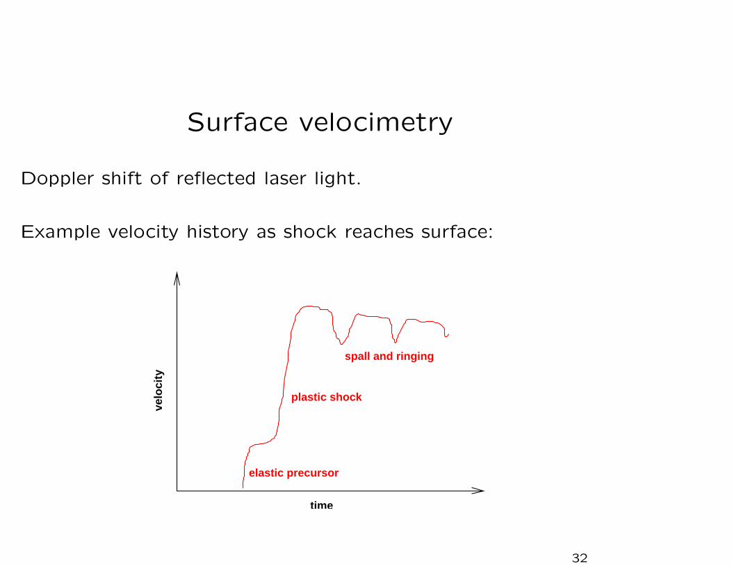
Surface velocimetry
Doppler shift of reflected laser light.
Example velocity history as shock reaches surface:
velo
city
time
elastic precursor
plastic shock
spall and ringing
32

Transient x-ray diffraction
Si crystal, (100) orientation, 40 µm thick by 10 mm across:
33

Quasi-isentropic compression
drive beamilluminates targetto generate dynamic load
plasma blowofffrom surfacesupports compression
loading wave
sample
compressed state
window(optional)
velocimetry
34

Quasi-isentropic compression
Si, TRIDENT shot 15018:
0
0.2
0.4
0.6
0.8
1
1.2
1.4
0 2 4 6 8 10 12 14
irrad
ianc
e (P
W/m
2 ), v
eloc
ity (
km/s
)
time (ns)
laser irradiance
free surface velocity
30 µm 59 µm
35
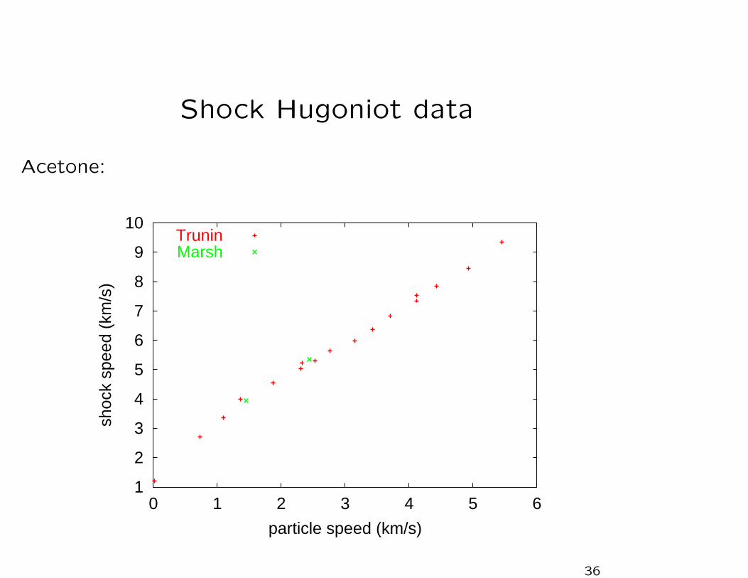
Shock Hugoniot data
Acetone:
1
2
3
4
5
6
7
8
9
10
0 1 2 3 4 5 6
shoc
k sp
eed
(km
/s)
particle speed (km/s)
TruninMarsh
36

Empirical mechanical EOSFunctional fit to us – up data, e.g. Steinberg polynomial:
us = c0 +
n∑
i=1
si
(
up
us
)i−1
up,
R-H relations for states on the Hugoniot. Additional assumption to calculatestates off-Hugoniot: Gruneisen approximation,
p(ρ, e) = pref(ρ) + Γ(ρ)[
e − eref(ρ)]
.
Thus
p(ρ, e) =F (ρ, e)
H2(ρ, e)+ [Γ0 + bµ(ρ)] ρ0e
where µ(ρ) = ρ/ρ0 − 1,
F (ρ, e) = ρ0c20µ {1 + µ [(1 − Γ0/2) − µb/2]}
H(ρ, e) = 1 + µ − µ
[
n∑
i=1
si
(
µ
µ + 1
)i−1]
(thermodynamically incomplete).
37
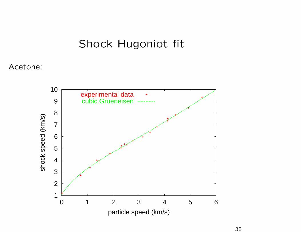
Shock Hugoniot fit
Acetone:
1
2
3
4
5
6
7
8
9
10
0 1 2 3 4 5 6
shoc
k sp
eed
(km
/s)
particle speed (km/s)
experimental datacubic Grueneisen
38

Accuracy of empirical EOS
Shock Hugoniot for solid and porous Al; empirical EOS fitted
to us – up; Γ(ρ) estimated from slope of us – up:
0
2
4
6
8
10
12
0 1 2 3 4 5
shoc
k sp
eed
(km
/s)
particle speed (km/s)
2.785 g/cm3
2.50 g/cm3
2.25 g/cm3
2.00 g/cm3
1.70 g/cm3
39

Accuracy of empirical EOS
Shock Hugoniot for solid and porous Al; empirical EOS fitted
to us – up; Γ(ρ) adjusted to reproduce porous Hugoniot points:
0
2
4
6
8
10
12
0 1 2 3 4 5
shoc
k sp
eed
(km
/s)
particle speed (km/s)
2.785 g/cm3
2.50 g/cm3
2.25 g/cm3
2.00 g/cm3
1.70 g/cm3
40

Accuracy of theoretical EOS
Shock Hugoniot for solid and porous Al; theoretical EOS uses
ab initio quantum mechanics:
0
2
4
6
8
10
12
0 1 2 3 4 5
shoc
k sp
eed
(km
/s)
particle speed (km/s)
2.785 g/cm3
2.50 g/cm3
2.25 g/cm3
2.00 g/cm3
1.70 g/cm3
41
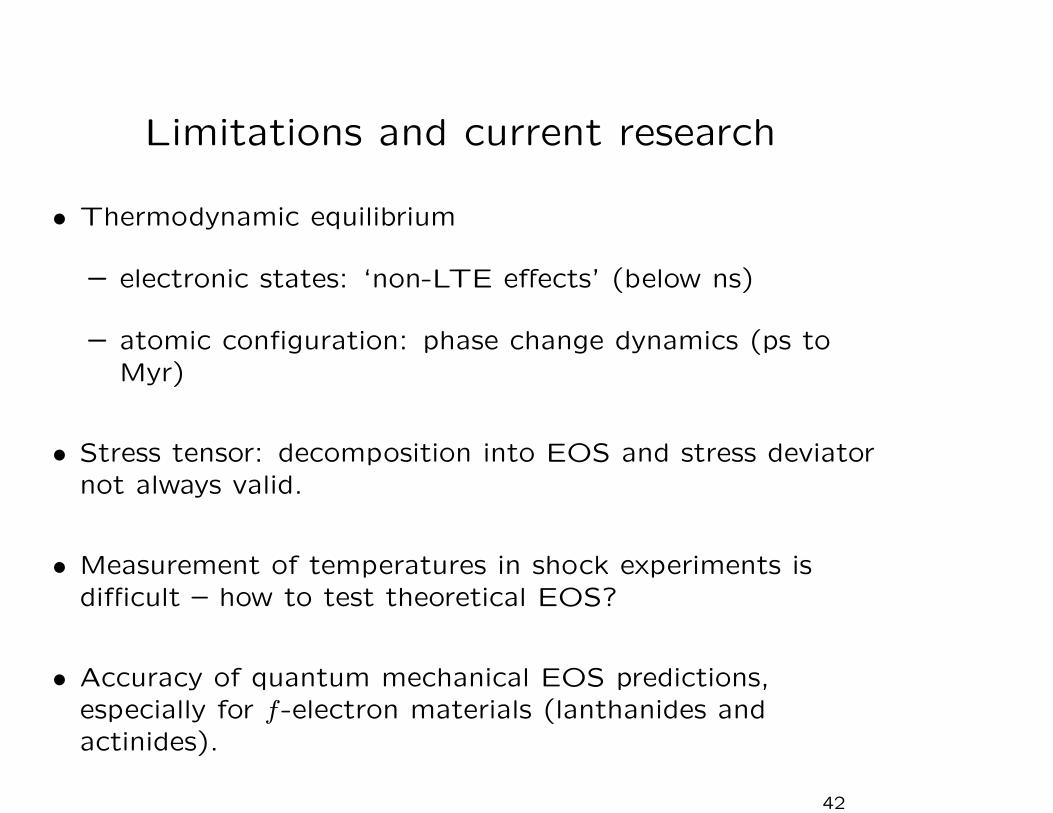
Limitations and current research
• Thermodynamic equilibrium
– electronic states: ‘non-LTE effects’ (below ns)
– atomic configuration: phase change dynamics (ps to
Myr)
• Stress tensor: decomposition into EOS and stress deviatornot always valid.
• Measurement of temperatures in shock experiments is
difficult – how to test theoretical EOS?
• Accuracy of quantum mechanical EOS predictions,especially for f-electron materials (lanthanides and
actinides).
42
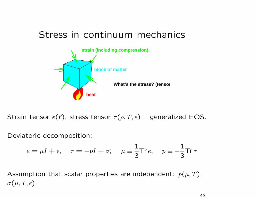
Stress in continuum mechanics
strain (including compression)
block of matter
heat
What’s the stress? (tensor)
Strain tensor e(~r), stress tensor τ(ρ, T, e) – generalized EOS.
Deviatoric decomposition:
e = µI + ε, τ = −pI + σ; µ ≡ 1
3Tr e, p ≡ −1
3Tr τ
Assumption that scalar properties are independent: p(µ, T ),
σ(µ, T, ε).
43

Uniqueness of the EOS
QM prediction of stress tensor in Be for different elastic strains:
-0.2
-0.1
0
0.1
0.2
0.3
0.4
0.5
0.6
1 1.1 1.2 1.3 1.4 1.5 1.6 1.7 1.8
mea
n pr
essu
re (
eV/A
3 )
mass density (amu/A3)
a=2.29 Aa=2.20 A
D.C. Swift and G.J. Ackland, Appl. Phys. Lett. 86, 6 (2003).
– at the end of the day, the EOS may not really exist!
44