Equilibria in the Tangle

Serguei Popov1,∗ Olivia Saa2 Paulo Finardi3

March 12, 2018

1Department of Statistics, Institute of Mathematics, Statistics and Scientific Computation, Uni-versity of Campinas – UNICAMP, rua Sergio Buarque de Holanda 651, 13083–859, Campinas SP,Brazile-mails: popov@ime.unicamp.br and serguei.popov@iota.org2Department of Applied Mathematics, Institute of Mathematics and Statistics, University of Sao

Paulo – USP, rua do Matao 1010, 05508–090, Sao Paulo SP, Brazile-mail: olivia@ime.usp.br and olivia.saa@iota.org3Institute of Computing – IC, University of Campinas – UNICAMP, av. Albert Einstein 1251,

13083–852, Campinas SP, Brazile-mails: ra144809@ic.unicamp.br and paulo.finardi@iota.org

Abstract

We analyse the Tangle — a DAG-valued stochastic process where new ver-tices get attached to the graph at Poissonian times, and the attachment’s loca-tions are chosen by means of random walks on that graph. These new vertices(also thought of as “transactions”) are issued by many players (which are thenodes of the network), independently. We prove existence of (“almost symmet-ric”) Nash equilibria for the system where a part of players tries to optimizetheir attachment strategies. Then, we also present simulations that show thatthe “selfish” players will nevertheless cooperate with the network by choosingattachment strategies that are similar to the “recommended” one.

Keywords: random walk, Nash equilibrium, directed acyclic graph, cryp-tocurrency, tip selection

AMS 2010 subject classifications: Primary 91A15. Secondary 60J20,68M14.

∗corresponding author

1

arX

iv:1

712.

0538

5v2

[m

ath.

PR]

9 M

ar 2

018

1 Introduction

In this paper we study the Tangle, a stochastic process on the space of (rooted)Directed Acyclic Graphs (DAGs). This process “grows” in time, in the sense thatnew vertices are attached to the graph according to a Poissonian clock, but no ver-tices/edges are ever deleted. When that clock rings, a new vertex appears and at-taches itself to locations that are chosen with the help of certain random walks onthe state of the process in the recent past (this is to model the network propagationdelays); these random walks therefore play the key role in the model.

Random walks on random graphs can be thought of as a particular case of Ran-dom Walks in Random Environments: here, the transition probabilities are functionsof the graph only, i.e., there are no additional variables (such as conductances1 etc.)attached to the vertices and/or edges of the graph. Still, this subject is very broad,and one can find many related works in the literature. One can mention the in-ternal DLA models (e.g. [13] and references therein), random walks on Erdos-Renyigraphs [5, 13], or random walks on the preferential attachment graphs [4] (which mostclosely resembles the model of this paper).

The motivation for studying the particular model presented in this paper stemsfrom the fact that it is applied in the IOTA cryptocurrency [1, 19], which uses (non-trivial) DAGs as the primary ledger for the transactions’ data. This is different from“traditional” cryptocurrencies such as the Bitcoin, where that data is stored in asequence of blocks2, also known as blockchain. An important observation, which mo-tivates the use of more general DAGs instead of blockchains is that the latter scalepoorly: when the network is large, it is difficult for it to achieve consensus on whichblocks are “valid” in the situations when the new blocks come too frequently. Wealso cite [2, 3, 16, 20] which deal with other approaches to using DAGs as distributedledgers.

The main results of the present paper deal with the following question: whatif some participants of the network are trying to minimize their costs by adoptinga behavior different from the “default” one? How will the system behave in suchcircumstances? To address these kinds of questions, we first provide general argu-ments to prove existence of (“almost symmetric”) Nash equilibria for the system, seeSection 2. Although one can hardly access the explicit form of these equilibria ina purely analytical way, simulations presented in Section 3 show that the “selfish”players will typically still choose attachment strategies that are similar to the default

1this refers to the well-known relation between reversible Markov chains and electric networks,see e.g. the classical book [7]

2that is, the underlying graph is essentially Z+ (after discarding finite forks)

2

one, meaning that they would prefer cooperating with the network rather than simplyusing it).

Let us stress also that, in this paper, we consider only “selfish” players (thosewho only care about their own costs but still want to use the network in a legitimateway3); we do not consider the case when there are “malicious” ones (those who wantto disrupt the network even at a cost to themselves). We are going to treat severaltypes of attacks against the network in the subsequent papers.

1.1 Description of the model

In the following we introduce the mathematical model describing the Tangle [19].Let card(A) stand for the cardinality of (multi)set A. For an oriented multigraph

T = (V,E), where V is the set of vertices and E is the multiset of edges, and v ∈ V ,we denote by

degin(v) = card{e = (u1, u2) ∈ E : u2 = v},degout(v) = card{e = (u1, u2) ∈ E : u1 = v}

the “incoming” and “outgoing” degrees of the vertex v (counting the multiple edges).In the following, we refer to multigraphs simply as graphs. For u, v ∈ V , we saythat u approves v, if (u, v) ∈ E. We use the notation A(u) for the set of the verticesapproved by u. We say that u ∈ V references v ∈ V if there is a sequence of sitesu = x0, x1, . . . , xk = v such that xj ∈ A(xj−1) for all j = 1, . . . , k, i.e., there is adirected path from u to v. If degin(w) = 0 (i.e., there are no edges pointing to w),then we say that w ∈ V is a tip.

Let G be the set of all directed acyclic graphs (also known as DAGs, that is,oriented graphs without cycles) G = (V,E) with the following properties:

• the graph G is finite and the multiplicity of any edge is at most two (i.e., thereare at most two edges linking the same vertices);

• there is a distinguished vertex ℘ ∈ V such that degout(v) = 2 for all v ∈ V \{℘},and degout(℘) = 0 (this vertex ℘ is called the genesis);

• any v ∈ V such that v 6= ℘ references ℘; that is, there is an oriented path4

from v to ℘ (one can say that the graph is connected towards ℘).

3i.e., want to issue valid transactions and have them confirmed by the rest of the network4not necessarily unique

3

We now describe the tangle as a continuous-time Markov process on the space G.The state of the tangle at time t ≥ 0 is a DAG T (t) = (VT (t), ET (t)), where VT (t) isthe set of vertices and ET (t) is the multiset of directed edges at time t. The process’sdynamics are described in the following way:

• The initial state of the process is defined by VT (0) = ℘, ET (0) = ∅.

• The tangle grows with time, that is, VT (t1) ⊂ VT (t2) and ET (t1) ⊂ ET (t2)whenever 0 ≤ t1 < t2.

• For a fixed parameter λ > 0, there is a Poisson process of incoming transactions ;these transactions then become the vertices of the tangle.

• Each incoming transaction chooses5 two vertices v′ and v′′ (which, in general,may coincide), and we add the edges (v, v′) and (v, v′′). We say in this casethat this new transaction was attached to v′ and v′′ (equivalently, v approves v′

and v′′).

• Specifically, if a new transaction v arrived at time t′, then VT (t′+) = VT (t′)∪{v},and ET (t′+) = ET (t) ∪ {(v, v′), (v, v′′)}.

Let us write

P(t)(x) ={y ∈ T (t) : y is referenced by x

},

F (t)(x) ={z ∈ T (t) : z references x

}for the “past” and the “future” with respect to x (at time t). Note that these introducea partial order structure on the tangle. Observe that, if t0 is the time moment when xwas attached to the tangle, then P(t)(x) = P(t0)(x) for all t ≥ t0. We also define the

cumulative weight H(t)x of the vertex x at time t by

H(t)x = 1 + card

(F (t)(x)

); (1)

that is, the cumulative weight of x is one (its “own weight”) plus the number of

vertices that reference it. Observe that, for any t > 0, if y approves x then H(t)x −

H(t)y ≥ 1, and the inequality is strict if and only if there are vertices different from y

which also approve x. Also note that the cumulative weight of any tip is equal to 1.There is some data associated to each vertex (transaction), created at the moment

when that transaction was attached to the tangle. The precise nature of that data is

5the precise selection mechanism will be described below

4

not relevant for the purposes of this paper, so we assume that it is an element of some(unspecified, but finite) set D; what is important, however, is that there is a naturalway to say if the set of vertices is consistent with respect to the data they contain6.When it is necessary to emphasize that the vertices of G ∈ G contain some data, weconsider the marked DAG G[d] to be (G, d) = (V,E, d), where d is a function V → D.We define G [d] to be the set of all marked DAGs (G, d), where G ∈ G.

1.2 Attachment strategies

There is one very important detail that has not been explained, namely: how doesa newly arrived transaction choose which two vertices in the tangle it will approve,i.e., what is the attachment strategy? Notice that, in principle, it would be good forthe whole system if the new transactions always prefer to select tips as attachmentplaces, since this way more transactions would be “confirmed”7. In any case, it isquite clear that the appropriate choice of the attachment strategy is essential for thecorrect functioning (whatever this could mean) of the system.

It is also important to comment that the attachment strategy of a network nodeis something “internal” to it; what others can see, are the attachment choices of thenode, but the mechanism behind them need not be publicly known. For this reason,an attachment strategy cannot be imposed in the protocol.

We now describe a possible choice of the attachment strategy, used to determinewhere the incoming transaction will be attached. It is also known as the recom-mended tip selection algorithm, since, due to reasons described above, the recom-mended nodes’ behavior is always to try to approve tips. We stress again, however,that approving only tips is not imposed in the protocol, since there is usually no wayto know if a node “knew” if the transaction it approved was already approved bysomeone else before (also, there is no way to know which approving transaction wasthe first).

Let us denote by L(t) the set of all vertices that are tips at time t, and let L(t) =card(L(t)). To model the network propagation delays, we introduce a parameter h >0, and assume that at time t only T (t − h) is known to the entity that issued theincoming transaction. We then define the tip-selecting random walk, in the followingway. It depends on a parameter q (the backtracking probability) and on a function f .

6one may think that the data refers to value transactions between accounts, and consistencymeans that no account has negative balance as a result, and/or the total balance has not increased

7we discuss the exact meaning of this later; for now, think that “confirmed” means “referencedby many other transactions”

5

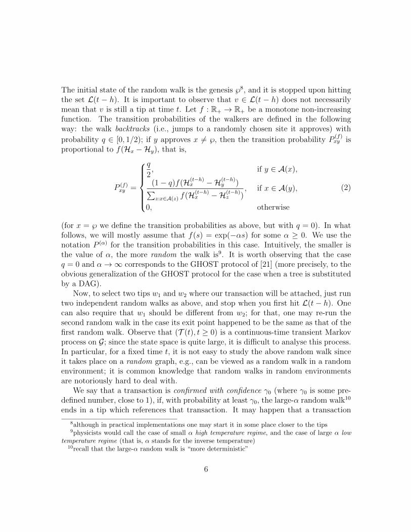
The initial state of the random walk is the genesis ℘8, and it is stopped upon hittingthe set L(t − h). It is important to observe that v ∈ L(t − h) does not necessarilymean that v is still a tip at time t. Let f : R+ → R+ be a monotone non-increasingfunction. The transition probabilities of the walkers are defined in the followingway: the walk backtracks (i.e., jumps to a randomly chosen site it approves) with

probability q ∈ [0, 1/2); if y approves x 6= ℘, then the transition probability P(f)xy is

proportional to f(Hx −Hy), that is,

P (f)xy =

q

2, if y ∈ A(x),

(1− q)f(H(t−h)x −H(t−h)

y )∑z:x∈A(z) f(H(t−h)

x −H(t−h)z )

, if x ∈ A(y),

0, otherwise

(2)

(for x = ℘ we define the transition probabilities as above, but with q = 0). In whatfollows, we will mostly assume that f(s) = exp(−αs) for some α ≥ 0. We use thenotation P (α) for the transition probabilities in this case. Intuitively, the smaller isthe value of α, the more random the walk is9. It is worth observing that the caseq = 0 and α→∞ corresponds to the GHOST protocol of [21] (more precisely, to theobvious generalization of the GHOST protocol for the case when a tree is substitutedby a DAG).

Now, to select two tips w1 and w2 where our transaction will be attached, just runtwo independent random walks as above, and stop when you first hit L(t− h). Onecan also require that w1 should be different from w2; for that, one may re-run thesecond random walk in the case its exit point happened to be the same as that of thefirst random walk. Observe that (T (t), t ≥ 0) is a continuous-time transient Markovprocess on G; since the state space is quite large, it is difficult to analyse this process.In particular, for a fixed time t, it is not easy to study the above random walk sinceit takes place on a random graph, e.g., can be viewed as a random walk in a randomenvironment; it is common knowledge that random walks in random environmentsare notoriously hard to deal with.

We say that a transaction is confirmed with confidence γ0 (where γ0 is some pre-defined number, close to 1), if, with probability at least γ0, the large-α random walk10

ends in a tip which references that transaction. It may happen that a transaction

8although in practical implementations one may start it in some place closer to the tips9physicists would call the case of small α high temperature regime, and the case of large α low

temperature regime (that is, α stands for the inverse temperature)10recall that the large-α random walk is “more deterministic”

6

℘

v0

u0

w0

Figure 1: The walk on the tangle and tip selection. Tips are circles, and transactionswhich were approved at least once are disks.

does not get confirmed (even, possible, does not get approved a single time), andbecomes orphaned forever. Let us define the event

U = {every transaction eventually gets approved}.

We believe that the following statement holds true; however, we have only aheuristical argument in its favor, not a rigorous proof. In any case, it is only oftheoretical interest, since, as explained below, in practice we will find ourselves in thesituation where P[U ] = 0. We therefore state it as

Conjecture 1.1. It holds that

P[U ] =

0, if

∫ +∞

0

f(s) ds <∞,

1, if

∫ +∞

0

f(s) ds =∞.(3)

Explanation. First of all, it should be true that P[U ] ∈ {0, 1} since U is a tail eventwith respect to the natural filtration; however, it does not seem to be very easy toprove the 0–1 law in this context (recall that we are dealing with a transient Markovprocess on an infinite state space). Next, consider a tip v0 which got attached to thetangle at time t0, and assume that it is still a tip at time t � t0; also, assume that,among all tips, v0 is “closest” (in some suitable sense) to the genesis. Let us nowthink of the following question: what is the probability that v0 will still be a tip attime t+ 1?

Look at Figure 1: during the time interval [t, t+1], O(1) new particles will arrive,and the corresponding walks will travel from the genesis ℘ looking for tips. Each ofthese walks will have to cross the dotted vertical segment on the picture, and withpositive probability at least one of them will pass through w0, one of the vertices

7

approved by v0. Assume that w0 was already confirmed (i.e., connected to the rightend of the tangle via some other transaction u0 that approves w0). Then, it is clear(but not easy to prove!) that the cumulative weight of both u0 and w0 should be O(t),and so, when in w0, the walk will jump to the tip v0 with probability f(O(t)).

This suggests that the probability that v0 ∈ L(t + 1) (i.e., that v0 still is tipat time t + 1) is f(O(t)), and the Borel-Cantelli lemma11 gives that the probabilitythat v0 will be eventually approved is less than 1 or equal to 1 depending on whether∑

n f(n) converges or diverges; the convergence (divergence) of the sum is equivalentto convergence (divergence) of the integral in (3) due to the monotonicity of the func-tion f . A standard probabilistic argument12 would then imply that if the probabilitythat a given tip remains orphaned forever is uniformly positive, then the probabilitythat at least one tip remains orphaned forever is equal to 1.

One may naturally think that it would be better to choose the function f in sucha way that, almost surely, every tip eventually gets confirmed. However, as explainedin Section 4.1 of [19], there is a good reason to choose a rapidly decreasing function f ,because this defends the system against nodes’ misbehavior and attacks. The idea isthen to assume that a transaction which did not get confirmed during a sufficientlylong period of time is “unlucky”, and needs to be reattached13 to the tangle. Letus fix some K > 0: it stands for the time when an unlucky transaction is reissued(because there is already very little hope that it would be confirmed “naturally”).We call a transaction issued less than K time units ago “unconfirmed”, and if atransaction was issued more than K time units ago and was not confirmed, we callit “orphaned”. In the following, we assume that the system is stable, in the sensethat the “recent” unconfirmed transactions do not accumulate and the time until atransaction is confirmed (roughly) does not depend on the moment when it appearedin the system14.

In that stable regime, let p be the probability that a transaction is confirmed Ktime units after it was issued for the first time; the number of times a transactionshould be issued to achieve confirmation is then a Geometric random variable withparameter p (and, therefore, with expected value p−1); so, the mean time until the

11to be precise, a bit more refined argument is needed since the corresponding events are notindependent

12which is also not so easy to formalize in these circumstances13in fact, the nodes of the network may adopt a rule that instructs to delete the transactions that

are older than K and still are tips from their databases14simulations indicate that this is indeed the case when α is small; however, it is not guaranteed

to happen for large values of α

8

transaction is confirmed is K/p. Let us then recall the following remarkable fact be-longing to the queuing theory, known as the Little’s formula (sometimes also referredto as the Little’s theorem or the Little’s identity):

Proposition 1.2. Suppose that λa is the arrival rate, µ is the mean number ofcustomers in the system, and T is the mean time a customer spends in the system.Then T = µ/λa.

Proof. See e.g. Section 5.2 of [6]. To understand intuitively why this fact holds true,one may reason in the following way: assume that, while in the system, each customerpays money to the system with rate 1. Then, at large time t, the total amount ofmoney earned by the system would be (approximately) µt on one hand, and Tλat onthe other hand. Dividing by t and then sending t to infinity, we obtain µ = Tλa.

Little’s formula then implies15 the following

Proposition 1.3. The average number of unconfirmed transactions in the system isequal to p−1λK.

Proof. Indeed, apply Proposition 1.2 with λa = λ (think of a transaction which wasreattached as a customer which returns to the server after an insuccessful serviceattempt; this way, the incoming flow of customers still has rate λ). As observedbefore, the mean time spent by a customer in the system is equal to K/p.

In case when the tangle contains data (which, in principle, can make transactionsincompatible between each other), one may choose more sophisticated methods of tipselection. As we already mentioned, selecting tips with larger values of α providesbetter defense against attacks and misbehavior; however, smaller values of α makethe system more stable with respect to the transactions’ confirmation times. Anexample of “mixed-α” strategy is the following. Define the “model tip” w0 as a resultof the random walk with large α, then select two tips w1 and w2 with random walkswith small α, but check that

P(t−h)(w0) ∪ P(t−h)(w1) ∪ P(t−h)(w2)

is consistent.

15in the language of queuing systems, a reissued transaction is a customer which goes back to theserver after an unsuccessful service attempt

9

2 Selfish nodes and Nash equilibria

Now, we are going to study the situation when some participants of the network are“selfish” and want to use a customized attachment strategy, in order to improve theconfirmation time of their transactions (possibly at the expense of the others).

For a finite set A let us denote byM(A) the set of all probability measures on A,that is

M(A) ={µ : A→ R such that µ(a) ≥ 0 for all a ∈ A and

∑a∈A

µ(a) = 1}.

LetM =

⋃G=(V,E)∈G

M(V × V )

be the union of the sets of all probability measures on the pairs of (not necessarilydistinct) vertices of DAGs belonging to G. Then, an attachment strategy S is a map

S : G [d] →M

with the property S(V,E, d) ∈ M(V × V ) for any G[d] = (V,E, d) ∈ G [d]; that is,for any G ∈ G with data attached to the vertices (which corresponds to the state ofthe tangle at a given time) there is a corresponding probability measure on the setof pairs of the vertices. Note also that in the above we considered ordered pairs ofvertices, which, of course, does not restrict the generality.

Let κ > 0 be a fixed number. We now assume that, for a (very) large N , thereare κN nodes that follow the default tip selection algorithm, and N “selfish” nodesthat try to minimize their “cost”, whatever this could mean16. Assume that allnodes issue transactions with the same rate λ

(κ+1)N, independently. The overall rate

of “honest” transactions in the system is then equal to λκκ+1

, and the overall rate of

transactions issued by selfish nodes equals λκ+1

.Let S1, . . . ,SN be the attachment strategies used by the selfish nodes. To evaluate

the “goodness” of a strategy, one has to choose and then optimize some suitableobservable (that stands for the “cost”); as usual, there are several “reasonable” waysto do this. We decided to choose the following one, for definiteness and also fortechnical reasons (to guarantee the continuity of some function used below); one can

16for example, the cost may be the expected confirmation time of a transaction (conditioned thatit is eventually confirmed), the probability that it was not approved during certain (fixed) timeinterval, etc.

10

probably extend our arguments to other reasonable cost functions. Assume that atransaction v was attached to the tangle at time tv, so v ∈ T (t) for all t ≥ tv. Fix

some (typically large) M0 ∈ N. Let t(v)1 , . . . , t

(v)M0

be the moments when the subsequent

(after v) transactions were attached to the tangle. For k = 1 . . . ,M0 let R(v)k be the

event that the default tip-selecting walk17 on T(t(v)k

)stops in a tip that does not

reference v. We then define

W (v) = 1R

(v)1

+ · · ·+ 1R

(v)M0

(4)

to be the number of times that the M0 “subsequent” tip selection random walks do notreference v (in the above, 1A is the indicator function of an event A). Intuitively, thesmaller is the value of W (v)/M0, the bigger is the chance that v is quickly confirmed.

Next, assume that (v(k)j , j ≥ 1) are the transactions issued by the kth (selfish)

node. We define

C(k)(S1, . . . ,SN) = M−10 lim

n→∞

W (v(k)1 ) + · · ·+W (v

(k)n )

n, (5)

to be the mean cost of the kth node given that S1, . . . ,SN are the attachment strate-gies of the selfish nodes.

Definition 2.1. We say that a set of strategies (S1, . . . ,SN) is a Nash equilibriumif

C(k)(S1, . . . ,Sk−1,Sk,Sk+1, . . . ,SN) ≤ C(k)(S1, . . . ,Sk−1,S ′,Sk+1, . . . ,SN)

for any k and any S ′ 6= Sk.

Observe that, since the nodes are indistinguishable, the fact that (S1, . . . ,SN) isa Nash equilibrium implies that so is (Sσ1 , . . . ,Sσ(N)) for any permutation σ.

Naturally, we would like to prove that Nash equilibria exist. Unfortunately, wecould not obtain the proof of this fact in the general case, since the space of all possiblestrategies is huge. Therefore, we consider the following simplifying assumption (whichis, by the way, also quite reasonable since, in practice, one would hardly use the genesisas the starting vertex for the random walks due to runtime issues):

Assumption L. There is n1 > 0 such that the attachment strategies of all nodes (in-cluding those that use the default attachment strategy) only depend on the restrictionof the tangle to the last n1 transactions that they see.

17i.e., the one used by nodes following the default attachment strategy

11

Observe that, under the above assumption, the set of all such strategies can bethought of as a compact convex subset of Rd, where d = d(n1) is sufficiently large.Additionally, we assume that the actual set of strategies that can be used by thenodes may be further restricted to some compact convex subset of the above subset.Also, observe that the set of all possible restrictions of elements of G on a subset of n1

vertices is finite; we denote that set by Gn1 . The set of all such attachments strategieswill be then denoted by Mn1 .

In this section we use a different approach to model the network propagationdelays: instead of assuming that an incoming transaction does not have informationabout the state of the tangle during last h units of time, we rather assume that it doesnot have information about the last n0 transactions attached to the tangle, where n0 <n1 is some fixed positive number (so, effectively, the strategies would depend onsubgraphs induced by n1−n0 transactions, although the results of this section do notrely on this assumption). Clearly, these two approaches are quite similar in spirit;however, the second one permits us to avoid certain technical difficulties related torandomness of the number of unseen transactions in the first case18.

From now on, we assume that vertices contain no data, i.e., the set D is empty;this is not absolutely necessary because, with the data, the proof will be essentiallythe same; however, the notations would become much more cumbersome. Also, therewill be no reattachments; again, this would unnecessarily complicate the proofs (onewould have to work with decorated Poisson processes). In fact, we are dealing with aso-called random-turn game here (see e.g. Chapter 9 of [15] for other examples).

To proceed, we need the following

Lemma 2.2. Let P be the transition matrix of an irreducible and aperiodic discrete-time Markov chain on a finite state space E. Let P be a continuous map from acompact set F ⊂ Rd to the set of all stochastic matrices on E (equipped by thedistance inherited from the usual matrix norm on the space of all matrices on E).

Fix θ ∈ (0, 1), denote P (s) = θP + (1− θ)P (s), and let πs be the (unique) stationary

measure of P (s). Then, the map s 7→ πs is also continuous.

Proof. In the following we give a (rather) probabilistic proof of this fact via the Kac’slemma, although, of course, a purely analytic proof is also possible. Irreducibility andaperiodicity of P imply that, for some m0 ∈ N and ε0 > 0

Pm0xy ≥ ε0 (6)

18also, it will be more natural and convenient to pass from continuous to discrete time

12

for all x, y ∈ E. Now, (6) implies that

Pm0xy (s) ≥ θm0ε0 (7)

for all x, y ∈ E and all s ∈ F .Being (Xn, n ≥ 0) a stochastic process on E, let us define

τ(x) = min{k ≥ 1 : Xk = x}(with the convention min ∅ = ∞) to be the hitting time of the site x ∈ E by the

stochastic process X. Now, let P(s)x and E(s)

x be the probability and the expectationwith respect to the Markov chain with transition matrix P (s) starting from x ∈ E.We now recall the Kac’s lemma (cf. e.g. Theorem 1.22 of [8]): for all x ∈ E it holdsthat

πs(x) =1

E(s)x τ(x)

. (8)

Now, (7) readily implies that, for all x ∈ E and n ∈ N,

P(s)x [τ(x) ≥ n] ≤ c1e

−c2n (9)

for some positive constants c1,2 which do not depend on s. This in its turn impliesthat the series

E(s)x τ(x) =

∞∑n=1

P(s)x [τ(x) ≥ n]

converges uniformly in s and so E(s)x τ(x) is uniformly bounded from above19; also,

the Uniform Limit Theorem implies that E(s)x τ(x) is continuous in s. Therefore, for

any x ∈ E, (8) implies that πs(x) is also a continuous function of s.

Consider, for the moment, the situation when all nodes use the same (default)attachment strategy (i.e., there are no selfish nodes). The restriction of the tangleon the last n1 transactions then becomes a Markov chain on the state space Gn1 . Wenow make the following technical assumption on that Markov chain:

Assumption D. The above Markov chain is irreducible and aperiodic.

It is important to observe that Assumption D is not guaranteed to hold for everynatural attachment strategy; however, still, this is not a very restrictive assumptionin practice because every finite Markov chain may be turned into an irreducible andaperiodic one by an arbitrarily small perturbation of the transition matrix.

Then, we are able to prove the following

19and, of course, it is also bounded from below by 1

13

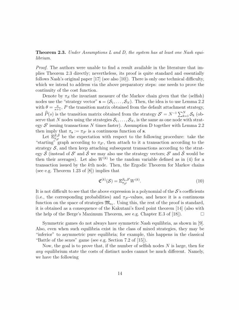
Theorem 2.3. Under Assumptions L and D, the system has at least one Nash equi-librium.

Proof. The authors were unable to find a result available in the literature that im-plies Theorem 2.3 directly; nevertheless, its proof is quite standard and essentiallyfollows Nash’s original paper [17] (see also [10]). There is only one technical difficulty,which we intend to address via the above preparatory steps: one needs to prove thecontinuity of the cost function.

Denote by πS the invariant measure of the Markov chain given that the (selfish)nodes use the “strategy vector” s = (S1, . . . ,SN). Then, the idea is to use Lemma 2.2with θ = κ

κ+1, P the transition matrix obtained from the default attachment strategy,

and P (s) is the transition matrix obtained from the strategy S ′ = N−1∑N

k=1 Sk (ob-serve that N nodes using the strategies S1, . . . ,SN , is the same as one node with strat-egy S ′ issuing transactions N times faster). Assumption D together with Lemma 2.2then imply that πs := πS′ is a continuous function of s.

Let ES,SπS′ be the expectation with respect to the following procedure: take the“starting” graph according to πS′ , then attach to it a transaction according to thestrategy S, and then keep attaching subsequent transactions according to the strat-egy S (instead of S ′ and S we may also use the strategy vectors; S ′ and S would bethen their averages). Let also W (k) be the random variable defined as in (4) for atransaction issued by the kth node. Then, the Ergodic Theorem for Markov chains(see e.g. Theorem 1.23 of [8]) implies that

C(k)(S) = ESk,S′πS′ W (k). (10)

It is not difficult to see that the above expression is a polynomial of the S’s coefficients(i.e., the corresponding probabilities) and πS′-values, and hence it is a continuousfunction on the space of strategies Mn1 . Using this, the rest of the proof is standard,it is obtained as a consequence of the Kakutani’s fixed point theorem [14] (also withthe help of the Berge’s Maximum Theorem, see e.g. Chapter E.3 of [18]).

Symmetric games do not always have symmetric Nash equilibria, as shown in [9].Also, even when such equilibria exist in the class of mixed strategies, they may be“inferior” to asymmetric pure equilibria; for example, this happens in the classical“Battle of the sexes” game (see e.g. Section 7.2 of [15]).

Now, the goal is to prove that, if the number of selfish nodes N is large, then forany equilibrium state the costs of distinct nodes cannot be much different. Namely,we have the following

14

Theorem 2.4. For any ε > 0 there exists N0 (depending on the default attachmentstrategy) such that, for all N ≥ N0 and any Nash equilibrium (S1, . . . ,SN) it holdsthat ∣∣C(k)(S1, . . . ,SN)− C(j)(S1, . . . ,SN)

∣∣ < ε (11)

for all k, j ∈ {1, . . . , N}.

Proof. Without restricting generality we may assume that

C(1)(S1, . . . ,SN) = maxk=1,...,N

C(k)(S1, . . . ,SN),

C(2)(S1, . . . ,SN) = mink=1,...,N

C(k)(S1, . . . ,SN),

so we then need to proof that C(1)(s)−C(2)(s) < ε, where s = (S1, . . . ,SN). Now, themain idea of the proof is the following: if C(1)(s) is considerably larger than C(2)(s),then the owner of the first node may decide to adopt the strategy used by the secondone. This would not necessarily decrease his costs to the (former) costs of the secondnode since a change in an individual strategy leads to changes in all costs; however,when N is large, the effects of changing the strategy of only one node would besmall, and (if the difference of C(1)(s) and C(2)(s) were not small) this would lead toa contradiction to the assumption that s was a Nash equilibrium.

So, let us denote s′ = (S2,S2,S3, . . . ,SN), the strategy vector after the first nodeadopted the strategy of its “more successful” friend. Let

S =1

N

(S1 + · · ·+ SN

)and S ′ = 1

N

(2S2 + S3 + · · ·+ SN

)be the two “averaged” strategies. In the following, we are going to compare C(2)(s) =

E(S2,S)πS W (2) (the “old” cost of the second node) with C(1)(s′) = E(S2,S′)

πS′ W (1) (the“new” cost of the first node, after it adopted the second node’s strategy). We needthe following

Lemma 2.5. For any measure π on Gn1 and any strategy vectors s = (S1, . . . ,SN)and s′ = (S ′1, . . . ,S ′N) such that Sk = S ′k for all k = 2, . . . , N , we have∣∣E(Sj ,S)

π W (j) − E(S′j ,S′)π W (j)

∣∣ ≤ M0

N(12)

for all j = 2, . . . , N .

15

Proof. Let us define the event

A = {among the M0 transactions there is at least one issued by the first node},

and observe that, by the union bound, the probability that it occurs is at most M0/N .

Then, using the fact that E(Sj ,S)π (W (j)1Ac) = E(Sj ,S′)

π (W (j)1Ac) (since, on Ac, the firstnode does not “contribute” to W (j)), write∣∣E(Sj ,S)

π W (j) − E(S′j ,S′)π W (j)

∣∣=∣∣E(Sj ,S)

π (W (j)1A) + E(Sj ,S)π (W (j)1Ac)− E(Sj ,S′)

π (W (j)1A)− E(Sj ,S′)π (W (j)1Ac)

∣∣=∣∣E(Sj ,S)

π (W (j)1A)− E(Sj ,S′)π (W (j)1A)

∣∣≤ M0

N,

where we also used that W (j) ≤ 1. This concludes the proof of Lemma 2.5.

We continue proving Theorem 2.4. First, by symmetry, we have

E(S2,S′)πS′ W (1) = E(S2,S′)

πS′ W (2). (13)

Also, it holds that ∣∣E(S2,S′)πS′ W (2) − E(S2,S)

πS′ W (2)∣∣ ≤ M0

N(14)

by Lemma 2.5. Then, similarly to the proof of Theorem 2.3, we can obtain that thefunction

(S,S ′,S ′′) 7→ E(S,S′)πS′′ W (2)

is continuous; since it is defined on a compact, it is also uniformly continuous. Thatis, for any ε′ > 0 there exist δ′ > 0 such that if ‖(S,S ′,S ′′)− (S, S ′, S ′′)‖ < δ′, then∣∣E(S,S′)

πS′′ W (2) − E(S,S′)πS′′ W (2)

∣∣ < ε′.

Choose N0 = d1/δ′e. We then obtain from the above that∣∣E(S2,S)πS′ W (2) − E(S2,S)

πSW (2)

∣∣ < ε′. (15)

The relations (13), (14), and (15) imply that∣∣E(S2,S′)πS′ W (1) − E(S2,S)

πSW (2)

∣∣ ≤ ε′ +M0

N.

16

On the other hand, since we assumed that s is a Nash equilibrium, it holds that

E(S2,S′)πS′ W (1) = C(1)(s′) ≥ C(1)(s) = E(S1,S)

πSW (1), (16)

which implies that

E(S1,S)πS

W (1) − E(S2,S)πS

W (2) ≤ ε′ +M0

N.

This concludes the proof of Theorem 2.4.

Now, let us define the notion of approximate Nash equilibrium:

Definition 2.6. For a fixed ε > 0, we say that a set of strategies (S1, . . . ,SN) is anε-equilibrium if

C(k)(S1, . . . ,Sk−1,Sk,Sk+1, . . . ,SN) ≤ C(k)(S1, . . . ,Sk−1,S ′,Sk+1, . . . ,SN) + ε

for any k and any S ′ 6= Sk.

The motivation for introducing this notion is that, if ε is very small, then, inpractice, ε-equilibria are essentially indistinguishable from the “true” Nash equilibria.

Theorem 2.7. For any ε > 0 there exists N0 (depending on the default attachmentstrategy) such that, for all N ≥ N0 and any Nash equilibrium (S1, . . . ,SN) it holdsthat (S, . . . ,S) is an ε-equilibrium, where

S =1

N

N∑k=1

S(k) (17)

(that is, all selfish nodes use the same “averaged” strategy defined above). The costsof all selfish nodes are then equal to

1

N

N∑k=1

C(k)(S1, . . . ,SN),

that is, the average cost in the Nash equilibrium.

In other words, for large N one can essentially assume that all selfish nodes followthe same attachment strategy.

17

Proof. To begin, we observe that the proof of the second part is immediate, since,as already noted before, for an external observer, the situation where there are Nnodes with strategies (S1, . . . ,SN) is indistinguishable from the situation with onenode with averaged strategy.

Now, we need to prove that, for any fixed ε′ > 0 it holds that

C(1)(S, . . . ,S) ≤ C(1)(S,S, . . . ,S) + ε′ (18)

for all large enough N (the claim would then follow by symmetry). Recall that wehave

C(1)(S, . . . ,S) = E(S,S)πS

W (1), (19)

C(1)(S1, . . . ,SN) = E(S1,S)πS

W (1), (20)

and

C(1)(S,S, . . . ,S) = E(S,S′)πS′ W (1), (21)

where

S ′ = 1

N

(S + (N − 1)S

)=

1

N

(S +

N − 1

N(S1 + · · ·+ SN)

).

Now, the second part of this theorem together with Theorem 2.4 imply20 that, forany fixed ε > 0 ∣∣E(S,S)

πSW (1) − E(S1,S)

πSW (1)

∣∣ < ε (22)

for all large enough N .Next, let us denote

S ′′ = 1

N(S + S2 + · · ·+ SN).

Then, again using the uniform continuity argument (as in the proof of Theorem 2.4),we obtain that, for any ε′′ > 0∣∣E(S,S′)

πS′ W (1) − E(S,S′′)πS′′ W (1)

∣∣ < ε′′ (23)

for all large enough N . However,

E(S,S′′)πS′′ W (1) = C(1)(S,S2, . . . ,SN) ≥ C(1)(S1,S2, . . . ,SN) = E(S1,S)

πSW (1),

since (S1, . . . ,SN) is a Nash equilibrium. Then, (22)–(23) imply that∣∣E(S,S)πS

W (1) − E(S,S′)πS′ W (1)

∣∣ < ε+ ε′′,

and, recalling (19) and (21), we conclude the proof of Theorem 2.7.20note that Theorem 2.4 implies that, when N is large, the nodes already have “almost” the same

cost in the Nash equilibrium (S1, . . . ,SN )

18

T (t) T (t + ∆)

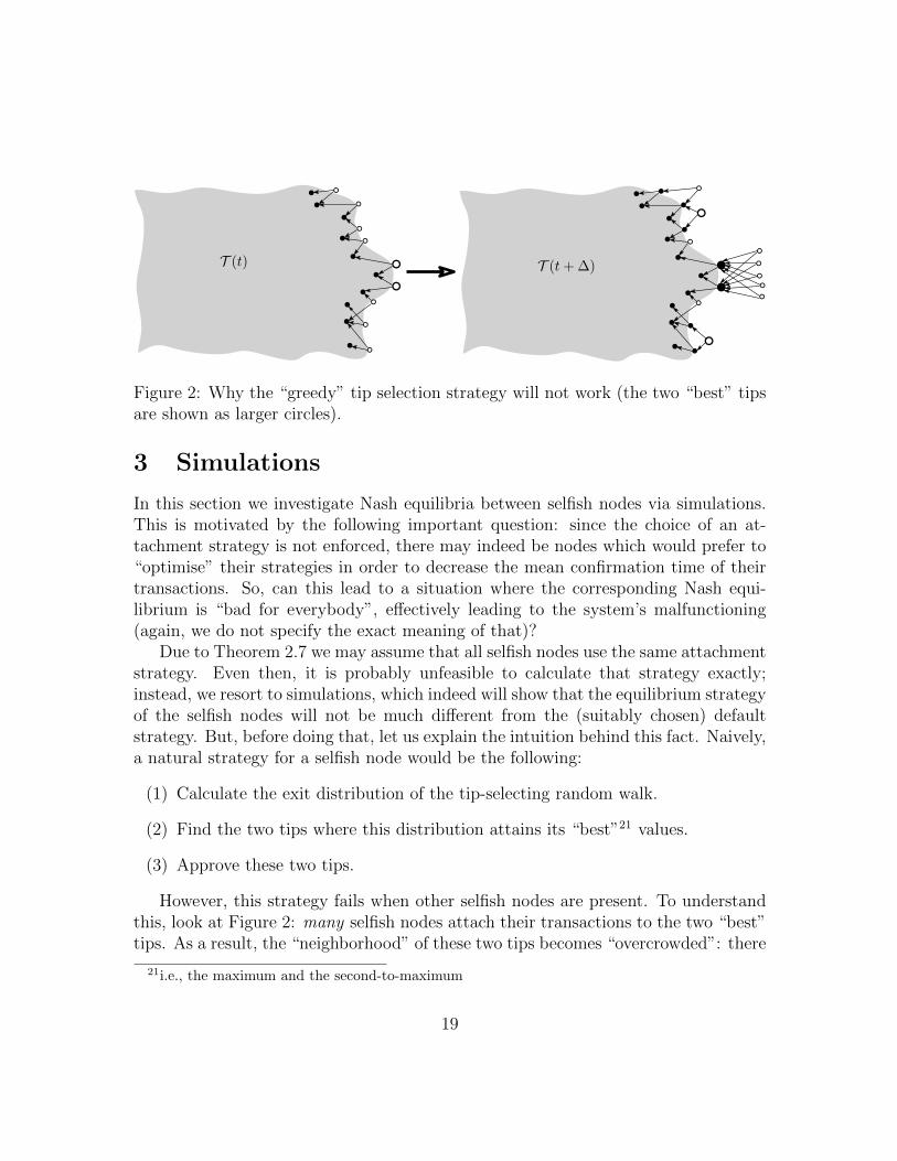
Figure 2: Why the “greedy” tip selection strategy will not work (the two “best” tipsare shown as larger circles).

3 Simulations

In this section we investigate Nash equilibria between selfish nodes via simulations.This is motivated by the following important question: since the choice of an at-tachment strategy is not enforced, there may indeed be nodes which would prefer to“optimise” their strategies in order to decrease the mean confirmation time of theirtransactions. So, can this lead to a situation where the corresponding Nash equi-librium is “bad for everybody”, effectively leading to the system’s malfunctioning(again, we do not specify the exact meaning of that)?

Due to Theorem 2.7 we may assume that all selfish nodes use the same attachmentstrategy. Even then, it is probably unfeasible to calculate that strategy exactly;instead, we resort to simulations, which indeed will show that the equilibrium strategyof the selfish nodes will not be much different from the (suitably chosen) defaultstrategy. But, before doing that, let us explain the intuition behind this fact. Naively,a natural strategy for a selfish node would be the following:

(1) Calculate the exit distribution of the tip-selecting random walk.

(2) Find the two tips where this distribution attains its “best”21 values.

(3) Approve these two tips.

However, this strategy fails when other selfish nodes are present. To understandthis, look at Figure 2: many selfish nodes attach their transactions to the two “best”tips. As a result, the “neighborhood” of these two tips becomes “overcrowded”: there

21i.e., the maximum and the second-to-maximum

19

is so much competition between the transactions issued by the selfish nodes, that thechances of them being approved soon actually decrease22.

To illustrate this fact, several simulations have been done. All the results depictedhere were generated using (2) as the transition probabilities, with q = 1/3, and anetwork delay of h = 1 second. Also, a transaction will be reattached if the twofollowing criteria are met:

(1) the transaction is older than 20 seconds23;

(2) the transaction is not referenced by the tip selected by a random walk withα =∞24.

This way, we guarantee not only that the unconfirmed transactions will be eventu-ally confirmed, but also that all transactions that were never reattached are referencedby most of the tips. Note that when the reattachment is allowed in the simulations,if a new transaction references an old, already reattached transaction together withits newly reissued counterpart, there will be a double spending. Even though theodds of that are low (since when a transaction is re-emitted, it will be old enoughto be almost never chosen by the random walk algorithm), a specific procedure wasincluded in the simulations in order to not allow double spendings.

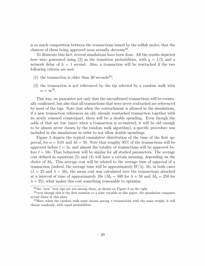
Figure 3 depicts the typical cumulative distribution of the time of the first ap-proval, for α = 0.01 and λh = 50. Note that roughly 95% of the transactions will beapproved before t = 5s, and almost the totality of transactions will be approved be-fore t = 10s. That behaviour will be similar for all studied parameters. The averagecost defined in equations (5) and (4) will have a certain meaning, depending on thechoice of M0. This average cost will be related to the average time of approval of atransaction (indeed, the average time will be approximately W/λ). So, in both cases(λ = 25 and λ = 50), the mean cost was calculated over the transactions attachedat a interval of time of approximately 10s (M0 = 500 for λ = 50 and M0 = 250 forλ = 25), what makes this cost something reasonable to optimise.

22the “new” best tips are not among them, as shown on Figure 2 on the right23even though this is the first mention to a time variable in this paper, the simulation compares

actual times at this place24Here, when the random walk must choose among n transactions with the same weight, it will

choose randomly, with equal probabilities

20

0 2 4 6 8 10Time of approval (s)

0.0

0.2

0.4

0.6

0.8

1.0

Like

lihood of occurrence

p=0.25p=0.05p=0

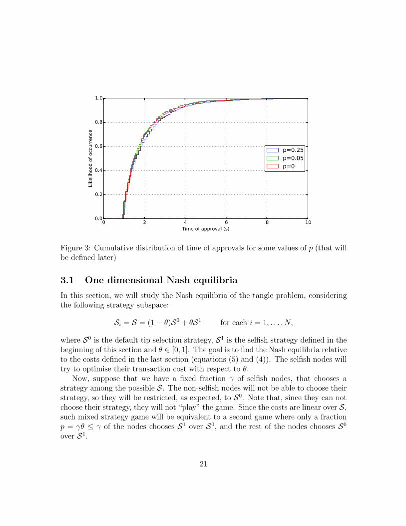
Figure 3: Cumulative distribution of time of approvals for some values of p (that willbe defined later)

3.1 One dimensional Nash equilibria

In this section, we will study the Nash equilibria of the tangle problem, consideringthe following strategy subspace:

Si = S = (1− θ)S0 + θS1 for each i = 1, . . . , N,

where S0 is the default tip selection strategy, S1 is the selfish strategy defined in thebeginning of this section and θ ∈ [0, 1]. The goal is to find the Nash equilibria relativeto the costs defined in the last section (equations (5) and (4)). The selfish nodes willtry to optimise their transaction cost with respect to θ.

Now, suppose that we have a fixed fraction γ of selfish nodes, that chooses astrategy among the possible S. The non-selfish nodes will not be able to choose theirstrategy, so they will be restricted, as expected, to S0. Note that, since they can notchoose their strategy, they will not “play” the game. Since the costs are linear over S,such mixed strategy game will be equivalent to a second game where only a fractionp = γθ ≤ γ of the nodes chooses S1 over S0, and the rest of the nodes chooses S0

over S1.

21

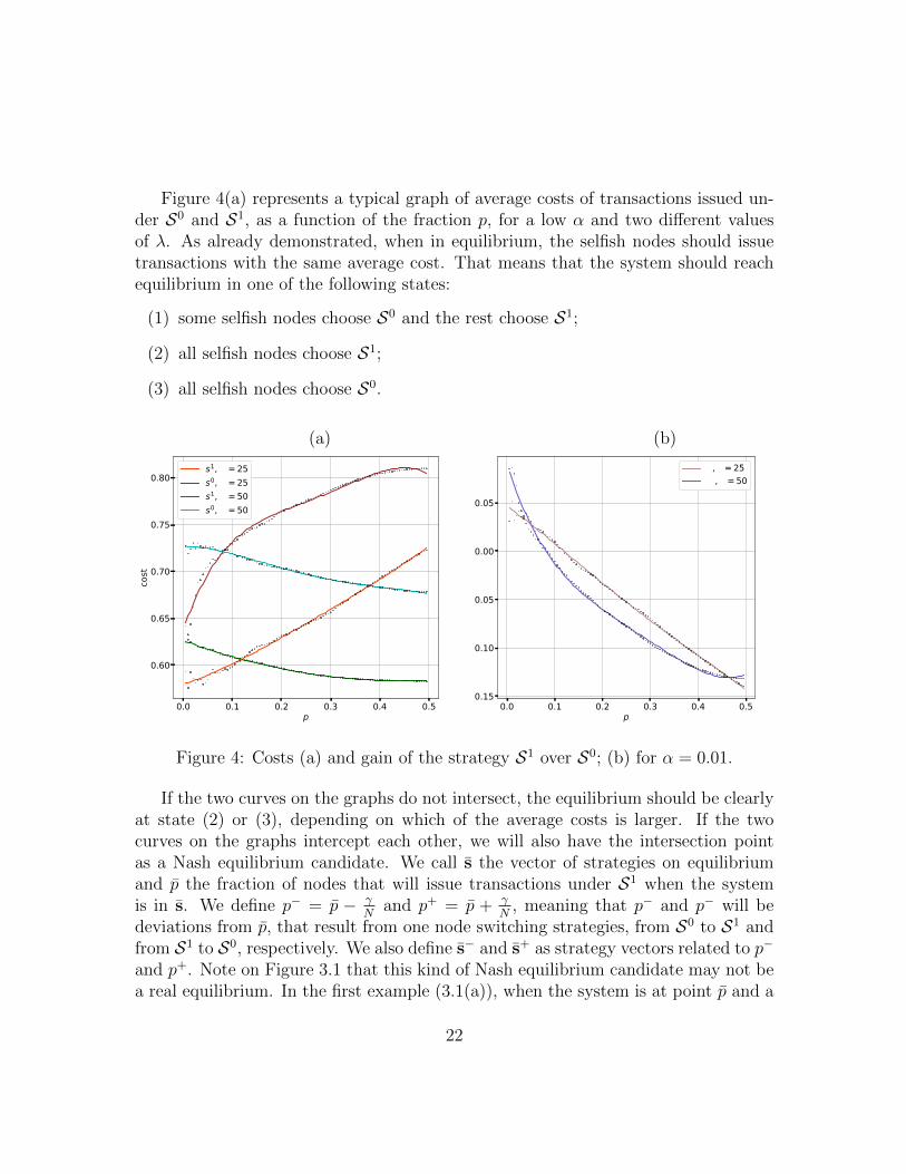
Figure 4(a) represents a typical graph of average costs of transactions issued un-der S0 and S1, as a function of the fraction p, for a low α and two different valuesof λ. As already demonstrated, when in equilibrium, the selfish nodes should issuetransactions with the same average cost. That means that the system should reachequilibrium in one of the following states:

(1) some selfish nodes choose S0 and the rest choose S1;

(2) all selfish nodes choose S1;

(3) all selfish nodes choose S0.

(a) (b)

0.0 0.1 0.2 0.3 0.4 0.5p

0.60

0.65

0.70

0.75

0.80

cost

s1, λ=25s0, λ=25s1, λ=50s0, λ=50

0.0 0.1 0.2 0.3 0.4 0.5p

−0.15

−0.10

−0.05

0.00

0.05

δδ, λ=25δ , λ=50

Figure 4: Costs (a) and gain of the strategy S1 over S0; (b) for α = 0.01.

If the two curves on the graphs do not intersect, the equilibrium should be clearlyat state (2) or (3), depending on which of the average costs is larger. If the twocurves on the graphs intercept each other, we will also have the intersection pointas a Nash equilibrium candidate. We call s the vector of strategies on equilibriumand p the fraction of nodes that will issue transactions under S1 when the systemis in s. We define p− = p − γ

Nand p+ = p + γ

N, meaning that p− and p− will be

deviations from p, that result from one node switching strategies, from S0 to S1 andfrom S1 to S0, respectively. We also define s− and s+ as strategy vectors related to p−

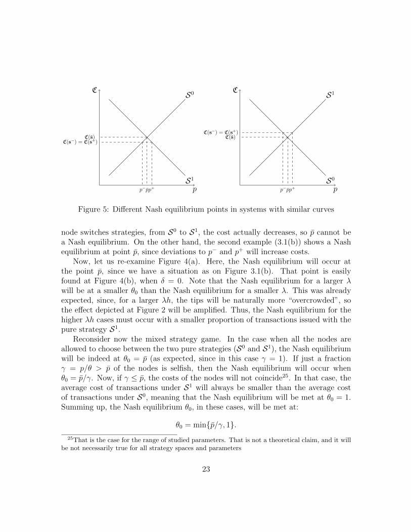
and p+. Note on Figure 3.1 that this kind of Nash equilibrium candidate may not bea real equilibrium. In the first example (3.1(a)), when the system is at point p and a

22

C

p

S0

S1

p−pp+

C(s)C(s−) = C(s+)

C

p

S1

S0

p−pp+

C(s)C(s−) = C(s+)

Figure 5: Different Nash equilibrium points in systems with similar curves

node switches strategies, from S0 to S1, the cost actually decreases, so p cannot bea Nash equilibrium. On the other hand, the second example (3.1(b)) shows a Nashequilibrium at point p, since deviations to p− and p+ will increase costs.

Now, let us re-examine Figure 4(a). Here, the Nash equilibrium will occur atthe point p, since we have a situation as on Figure 3.1(b). That point is easilyfound at Figure 4(b), when δ = 0. Note that the Nash equilibrium for a larger λwill be at a smaller θ0 than the Nash equilibrium for a smaller λ. This was alreadyexpected, since, for a larger λh, the tips will be naturally more “overcrowded”, sothe effect depicted at Figure 2 will be amplified. Thus, the Nash equilibrium for thehigher λh cases must occur with a smaller proportion of transactions issued with thepure strategy S1.

Reconsider now the mixed strategy game. In the case when all the nodes areallowed to choose between the two pure strategies (S0 and S1), the Nash equilibriumwill be indeed at θ0 = p (as expected, since in this case γ = 1). If just a fractionγ = p/θ > p of the nodes is selfish, then the Nash equilibrium will occur whenθ0 = p/γ. Now, if γ ≤ p, the costs of the nodes will not coincide25. In that case, theaverage cost of transactions under S1 will always be smaller than the average costof transactions under S0, meaning that the Nash equilibrium will be met at θ0 = 1.Summing up, the Nash equilibrium θ0, in these cases, will be met at:

θ0 = min{p/γ, 1}.25That is the case for the range of studied parameters. That is not a theoretical claim, and it will

be not necessarily true for all strategy spaces and parameters

23

(a) (b)

0.0 0.1 0.2 0.3 0.4 0.5p

0.55

0.60

0.65

0.70

0.75

0.80

0.85

0.90

cost

s1, λ=25s0, λ=25s1, λ=50s0, λ=50

0.0 0.1 0.2 0.3 0.4 0.5p

0.08

0.10

0.12

0.14

0.16

0.18

0.20

δ

δ, λ=25δ , λ=50

Figure 6: Costs (a) and gain (b) of the strategy S1 over S0; for α = 0.5.

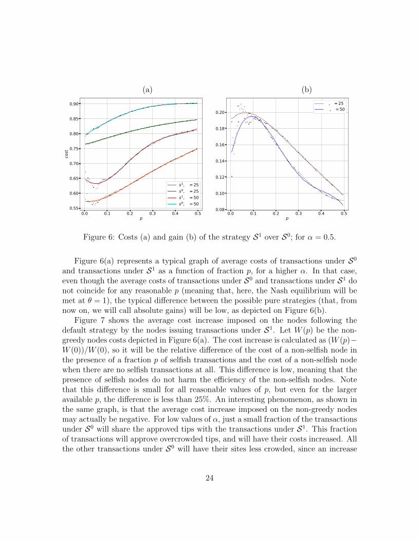
Figure 6(a) represents a typical graph of average costs of transactions under S0

and transactions under S1 as a function of fraction p, for a higher α. In that case,even though the average costs of transactions under S0 and transactions under S1 donot coincide for any reasonable p (meaning that, here, the Nash equilibrium will bemet at θ = 1), the typical difference between the possible pure strategies (that, fromnow on, we will call absolute gains) will be low, as depicted on Figure 6(b).

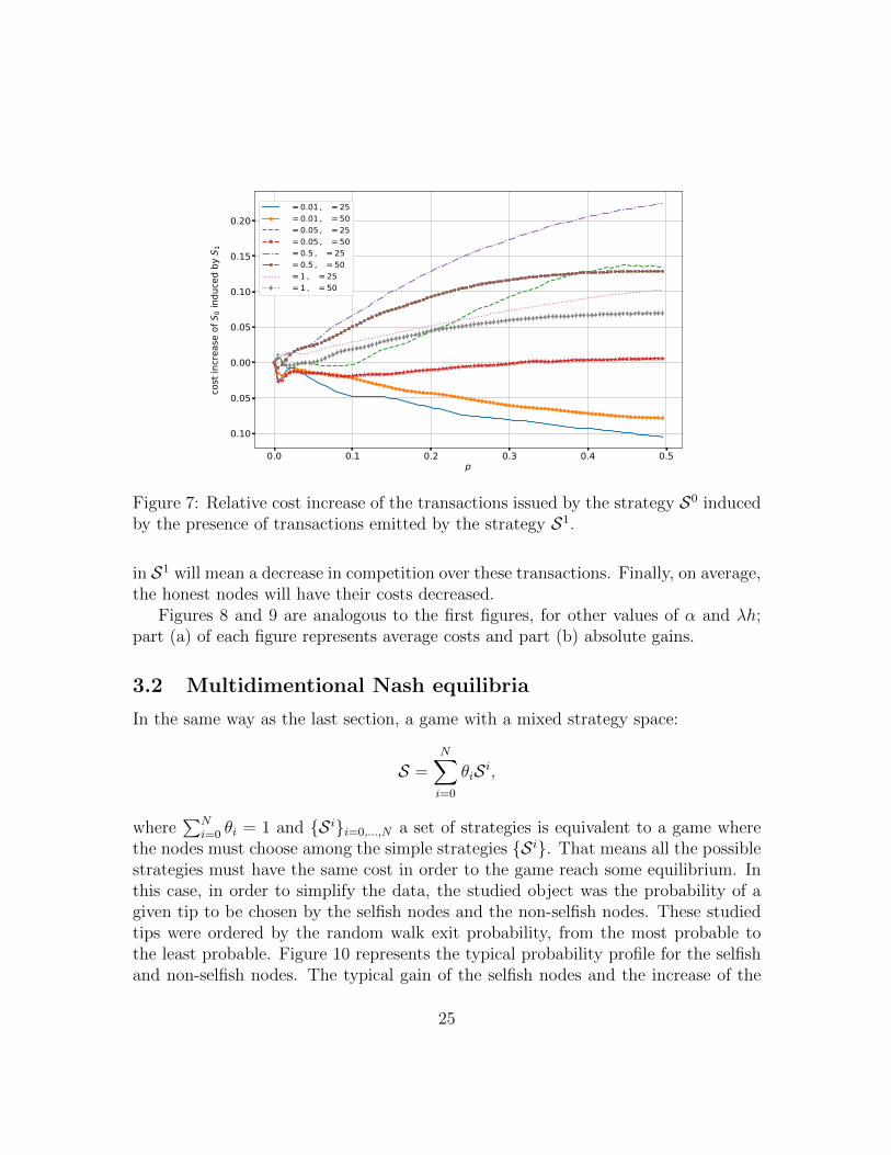
Figure 7 shows the average cost increase imposed on the nodes following thedefault strategy by the nodes issuing transactions under S1. Let W (p) be the non-greedy nodes costs depicted in Figure 6(a). The cost increase is calculated as (W (p)−W (0))/W (0), so it will be the relative difference of the cost of a non-selfish node inthe presence of a fraction p of selfish transactions and the cost of a non-selfish nodewhen there are no selfish transactions at all. This difference is low, meaning that thepresence of selfish nodes do not harm the efficiency of the non-selfish nodes. Notethat this difference is small for all reasonable values of p, but even for the largeravailable p, the difference is less than 25%. An interesting phenomenon, as shown inthe same graph, is that the average cost increase imposed on the non-greedy nodesmay actually be negative. For low values of α, just a small fraction of the transactionsunder S0 will share the approved tips with the transactions under S1. This fractionof transactions will approve overcrowded tips, and will have their costs increased. Allthe other transactions under S0 will have their sites less crowded, since an increase

24

0.0 0.1 0.2 0.3 0.4 0.5p

−0.10

−0.05

0.00

0.05

0.10

0.15

0.20co

st in

crea

se of S

0 ind

uced

by S 1

α=0.01 , λ=25α=0.01 , λ=50α=0.05 , λ=25α=0.05 , λ=50α=0.5 , λ=25α=0.5 , λ=50α=1 , λ=25α=1 , λ=50

Figure 7: Relative cost increase of the transactions issued by the strategy S0 inducedby the presence of transactions emitted by the strategy S1.

in S1 will mean a decrease in competition over these transactions. Finally, on average,the honest nodes will have their costs decreased.

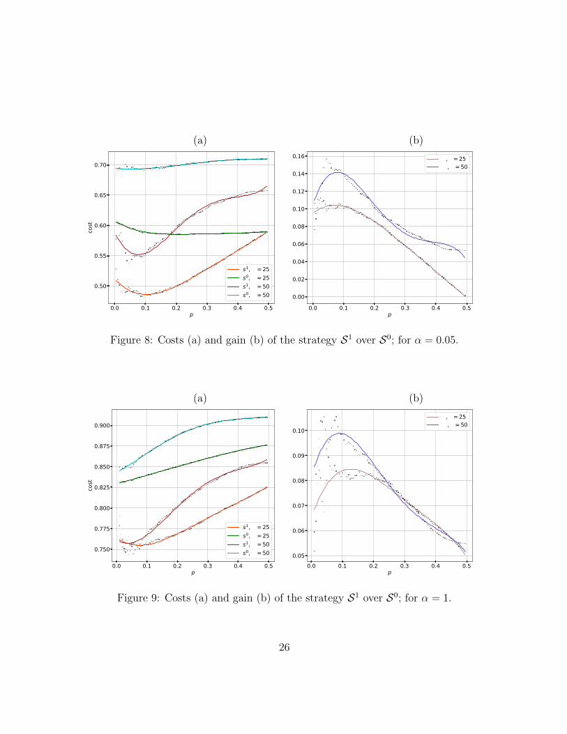
Figures 8 and 9 are analogous to the first figures, for other values of α and λh;part (a) of each figure represents average costs and part (b) absolute gains.

3.2 Multidimentional Nash equilibria

In the same way as the last section, a game with a mixed strategy space:

S =N∑i=0

θiS i,

where∑N

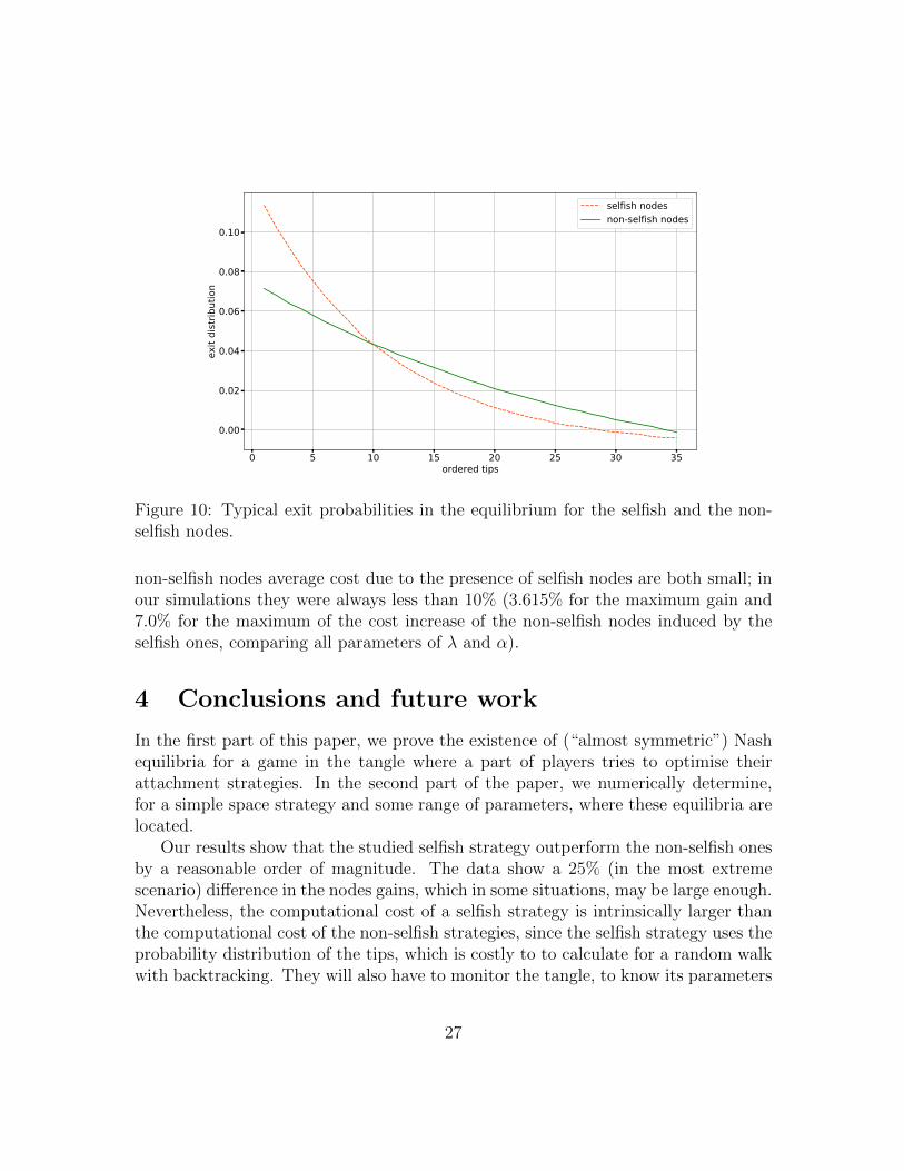
i=0 θi = 1 and {S i}i=0,...,N a set of strategies is equivalent to a game wherethe nodes must choose among the simple strategies {S i}. That means all the possiblestrategies must have the same cost in order to the game reach some equilibrium. Inthis case, in order to simplify the data, the studied object was the probability of agiven tip to be chosen by the selfish nodes and the non-selfish nodes. These studiedtips were ordered by the random walk exit probability, from the most probable tothe least probable. Figure 10 represents the typical probability profile for the selfishand non-selfish nodes. The typical gain of the selfish nodes and the increase of the

25

(a) (b)

0.0 0.1 0.2 0.3 0.4 0.5p

0.50

0.55

0.60

0.65

0.70

cost

s1, λ=25s0, λ=25s1, λ=50s0, λ=50

0.0 0.1 0.2 0.3 0.4 0.5p

0.00

0.02

0.04

0.06

0.08

0.10

0.12

0.14

0.16

δ

δ, λ=25δ , λ=50

Figure 8: Costs (a) and gain (b) of the strategy S1 over S0; for α = 0.05.

(a) (b)

0.0 0.1 0.2 0.3 0.4 0.5p

0.750

0.775

0.800

0.825

0.850

0.875

0.900

cost

s1, λ=25s0, λ=25s1, λ=50s0, λ=50

0.0 0.1 0.2 0.3 0.4 0.5p

0.05

0.06

0.07

0.08

0.09

0.10

δ

δ, λ=25δ , λ=50

Figure 9: Costs (a) and gain (b) of the strategy S1 over S0; for α = 1.

26

0 5 10 15 20 25 30 35ordered tips

0.00

0.02

0.04

0.06

0.08

0.10

exit distrib

ution

selfish nodesnon-selfish nodes

Figure 10: Typical exit probabilities in the equilibrium for the selfish and the non-selfish nodes.

non-selfish nodes average cost due to the presence of selfish nodes are both small; inour simulations they were always less than 10% (3.615% for the maximum gain and7.0% for the maximum of the cost increase of the non-selfish nodes induced by theselfish ones, comparing all parameters of λ and α).

4 Conclusions and future work

In the first part of this paper, we prove the existence of (“almost symmetric”) Nashequilibria for a game in the tangle where a part of players tries to optimise theirattachment strategies. In the second part of the paper, we numerically determine,for a simple space strategy and some range of parameters, where these equilibria arelocated.

Our results show that the studied selfish strategy outperform the non-selfish onesby a reasonable order of magnitude. The data show a 25% (in the most extremescenario) difference in the nodes gains, which in some situations, may be large enough.Nevertheless, the computational cost of a selfish strategy is intrinsically larger thanthe computational cost of the non-selfish strategies, since the selfish strategy uses theprobability distribution of the tips, which is costly to to calculate for a random walkwith backtracking. They will also have to monitor the tangle, to know its parameters

27

(like λ, h etc) and act accordingly. Also, even a extreme scenario, where almost halfof the transactions were issued by a selfish node, is not enough to harm the non-selfishones in a meaningful way.

On the other hand, our results raise further questions. The obtained data exhibita deep qualitative dependence on the parameter α of the simulation. This parameteris related to the randomness of the random walk (a low α implies a high randomness;a higher α implies a low randomness, meaning that the walk will be almost determin-istic). Further simulations will be done in order to study the effect of that variable inthe equilibria. Also, we only studied equilibria for a given cost, relative to the prob-ability of confirmation of the transactions in a certain interval of time. Since thisprobability depends heavily on the interval of time chosen (because the probabilitydistribution of the confirmations is far from uniform), another time intervals (thatwill have another practical meaning) must be analysed.

Finally, the equilibrium in the multidimensional strategy space should be studiedin a more quantitative and analytic way, since it should depend strongly on α and p;and until now it was studied in just a narrow range of parameters. Further researchwill also be done in order to optimise the default tip selection strategy in a way thatminimises this cost imposed by the selfish strategies. Through implementing researchmethods and techniques from the cross-reactive fields of measure theory, game theory,and graph theory, progress towards resolving the tangle-related open problems hasbeen well under way and will continue to be under investigation.

Acknowledgements

The authors thank Alon Gal, Gur Huberman, Bartosz Kumierz, John Licciardello,Samuel Reid, and Clara Shikhelman for valuable comments and suggestions.

References

[1] http://www.iota.org/

[2] L. Baird (2016) The Swirlds hashgraph consensus algorithm: fair, fast, Byzan-tine fault tolerance.http://www.swirlds.com/downloads/SWIRLDS-TR-2016-01.pdf

[3] A. Churyumov (2016) Byteball: a decentralized system for storage and transferof value. https://byteball.org/Byteball.pdf

28

[4] C. Cooper, A. Frieze (2007) The cover time of the preferential attachmentgraph. J. Comb. Theory B 97 (2), 269–290.

[5] C. Cooper, A. Frieze, S. Pett (2017) The covertime of a biased randomwalk on Gn,p. arXiv:1708.04908

[6] R.B. Cooper (1981) Introduction to Queueing Theory (2nd ed.). North Holland.

[7] P.G. Doyle, J.L. Snell (1984) Random walks and electric networks. CarusMathematical Monographs 22, Mathematical Association of America, Washing-ton.

[8] R. Durrett (2012) Essentials of Stochastic Processes (2nd. ed.) Springer.

[9] M. Fey (2012) Symmetric games with only asymmetric equilibria. Games Econ.Behavior 75 (1), 424–427.

[10] A.M. Fink (1964) Equilibrium in a stochastic n-person game. J. Sci. HiroshimaUniv. Ser. A-I Math. 28 (1), 89–93.

[11] A. Frieze, M. Krivelevich, P. Michaeli, R. Peled (2017) On the traceof random walks on random graphs. arXiv:1508.07355

[12] G. Iacobelli, D.R. Figueiredo, G. Neglia (2017) Transient and slim ver-sus recurrent and fat: random walks and the trees they grow. arXiv:1711.02913

[13] D. Jerison, L. Levine, S. Sheffield (2014) Internal DLA and the Gaussianfree field. Duke Math. J. 163 (2), 267–308.

[14] S. Kakutani (1941) A generalization of Brouwer’s fixed point theorem. DukeMath. J. 8 (3), 457–459.

[15] A.R. Karlin, Y. Peres (2017) Game Theory, Alive. American MathematicalSociety.

[16] S.D. Lerner (2015) DagCoin: a cryptocurrency without blocks.https://bitslog.wordpress.com/2015/09/11/dagcoin/

[17] J.F. Nash, Jr. (1950) Equilibrium points in n-person games. Proc. Natl. Acad.Sci. 36 (1), 48–49.

[18] E.A. Ok (2007) Real Analysis with Economics Applications. Princeton Univer-sity Press.

29

[19] S. Popov (2015) The tangle. https://iota.org/IOTA Whitepaper.pdf

[20] Y. Sompolinsky, Y. Lewenberg, A. Zohar (2016) SPECTRE: Serial-ization of proof-of-work events: confirming transactions via recursive elections.https://eprint.iacr.org/2016/1159.pdf

[21] Y. Sompolinsky, A. Zohar (2013) Secure high-rate transaction processing inBitcoin. https://eprint.iacr.org/2013/881.pdf

30