Equilibrium and optimal arrival patternsto a server with opening and closing times

Refael Hassin and 1 and Yana Kleiner 2

Abstract

We consider a first-come first-served single-server system with open-ing and closing times. Service durations are exponentially distributed,and the total number of arrivals is a Poisson random variable. Natu-rally each customer wishes to minimize his waiting time. The processof choosing an arrival time is presented as a (non-cooperative) multi-player game. Our goal is to find a Nash equilibrium game strategy.Glazer and Hassin (1983) assume that arrivals before the opening timeof the system are allowed. We study the case where early arrivals areforbidden. It turns out that unless the system is very heavily loaded,the equilibrium solution with such a restriction does not reduce theexpected waiting time in a significant way. We also compare the equi-librium solution with the solution which maximizes social welfare. Fi-nally, we show how social welfare can be increased in equilibrium byrestricting arrivals to certain points of time.

Keywords: Queues: Markovian, Non-stationary, Equilibrium Arrivals.

1 Introduction

Many real life service systems work in noncontinuous manner, having open-ing and closing times. Post office services, banks, government offices, li-braries, shops, drugstores, and bag drop-off services supplied by airlines arejust a few of these services. However, with only few exceptions, existingtheory assumes that service systems are continuously open to accept newarrivals.

A notable exception is the paper by Glazer and Hassin (1983); we adopttheir assumptions in this paper. The model considers a single-server sys-tem, which opens at time zero, closes at time T , and applies a first-comefirst-served discipline. All customers who arrive before closing time are ad-mitted to the queue, and the server is available to complete their service asnecessary. Customers choose their arrival times independently. Customersare indifferent to the exact time of the day they spend in the system, andtheir goal is to minimize their expected length of waiting time.

A central assumption in our model is that customers are free to choosetheir arrival time and have no preference to their exact time of service during

1School of Mathematical Sciences, Tel Aviv University, Tel Aviv 69978, Israel, has-sin@post.tau.ac.il Research supported by Israel Science Foundation Grant no. 526/08.

2School of Mathematical Sciences, Tel Aviv University, Tel Aviv 69978, Israel,yanaklei@post.tau.ac.il

1

the day. We discuss this full flexibility assumption and its implications inSection 3.3.

The waiting time of a customer is affected by the decisions of the othercustomers, and this turns the process into a non-cooperative multi-playergame. A strategy in this game is expressed by a density function givingthe probability distribution of arrival time for a random customer. Theequilibrium strategy, in general, is not optimal, in the sense that it doesn’tminimize the expected total waiting time of all customers. The reason isthat when deciding when to use the system, a user does not take into accountthe effect of his decision on the waiting time of other users (which is referredto as the external cost).

Assuming exponential service distribution and that the total numberof arrivals is a Poisson random variable, Glazer and Hassin compute theequilibrium arrival density. An important feature of this model is that earlyarrivals, that is, arrivals before opening time, are allowed.

A common way to reduce waiting time is by setting appointments. Theuse of appointments has been studied extensively, see for example Cayirliand Veral (2003). Such systems are commonly seen in health-care services,but not used by banking systems, for example.

In this paper we approximate the optimal density function, which min-imizes the expected waiting time over all arriving customers (it is not anequilibrium solution and therefore arrivals at different instants are associ-ated with different expected waiting time).

Since one usually cannot force customers to behave in a non-equilibriummanner, this solution cannot be implemented. However, one might stilltry to reduce the waiting time by restricting the instants when arrivals areadmitted. We consider two types of such restrictions. In the first, earlyarrivals are eliminated (for example by randomly ordering the customers attime 0). In the second, new arrivals are admitted only at a small set ofinstants. We show that such restrictions often make it possible to obtain anequilibrium with reduced expected waiting time.

The following illustrative example is a variation of the model, and theinsights we obtain can also help in finding ways to deal with such instances.The port of Haifa is located in the north of Israel. Trucks line up to obtaina container which they transport in most cases to the center of Israel, andthen return for another trip. Containers are released from 6am, at whichtime there is a very long line of trucks whose drivers arrived earlier to securea position in the line. After the first delivery of the day, trucks normallyreturn in the afternoon for another pickup. It is reasonable to assume thatdrivers are sufficiently flexible with respect to when they start their workingday, and that their main goal is to obtain a container at minimum wait aslong as it enables them to return for a second round. Is it possible to reducethe drivers waiting time by applying a random service order for all those

2

present at 6am?We show that eliminating early arrivals reduces the expected waiting

time significantly only when the system’s load is heavy (equivalently, theopening interval is short). However, when the server’s utilization is not verylow such a change will hardly save any waiting time. On the other hand, weshow how reduction in waiting can be achieved by other simple restrictionson the admission times of customers.

The paper is structured as follows. In Section 2 we survey relevantliterature. The queueing model is presented and the equilibrium is computedin Section 3. The optimal solution is studied in Section 4. In Section 5 wepresent numerical results and compare the models, and in Section 6 weanalyze restrictions of the arrivals to small sets of points. Finally, in Section7 we summarize our main results.

2 Literature Review

The model discussed in this paper is new and has not been studied in thisspecific form. However, it draws many similarities to previous results. Inthis paper we mention related models and discuss their relevance.

2.1 Transportation models

Research concerning equilibrium timing decisions was initiated in the con-text of transportation models. Vickrey (1969) described a deterministicmodel where commuters have complete knowledge about the other com-muters choice, and can change their home departure time to avoid periodsof high congestion. This simple model assumes a single bottleneck and afixed number of commuters. Delay occurs when the traffic flow exceeds thecapacity of the bottleneck. Each commuter has a preferred time to pass thebottleneck. There is a cost for arriving earlier than desired, and a cost fora late arrival. For later developments on this model see Lago and Daganzo(2007), Arnott (1999), Ostubo and Rapoport (2007), and their bibliogra-phies. A major difference between these models and our queueing model isthat we assume that customers do not have time preference and the equilib-rium we compute is symmetric. Moreover, congestion cannot be eliminated(though it can be alleviated) even when customers behave in a socially op-timal way.

2.2 Queueing models

The first queueing model where the arrival process is endogenously deter-mined is Glazer and Hassin (1983), as already described in the introduction.

Rapoport, Stein, Parco and Seale (2004) (see also, Bearden, Rapoportand Seale (2005)), considered a closely related discrete-time model of a

3

queueing system with pre-specified and commonly known opening and clos-ing times, a fixed and commonly known number of players, fixed servicetime, and no early arrivals. A player who arrives late and his service cannotbe completed before closing time is not served. A companion paper, Sealeet al. (2005), studies the same queueing system but allowing early arrivals.The papers compute equilibrium solutions and verify them experimentally.The experimental results indicate convergence to equilibrium with experi-ence in playing the game.

Glazer and Hassin (1987) compute equilibrium arrivals to a server withbatch service scheduled at published instants separated by intervals of aconstant length. Customers who arrive close to the beginning of servicemay face a full batch and need to wait for the next service time. This modelhas no opening and closing times, and what makes it non-stationary is thecommon knowledge of the fixed schedule.

Lariviere and Van Mieghem (2004) assume that each customer choosesa day within a given interval to arrive at a server. The waiting cost ismonotone increasing with the number of customers arriving on a particularday. Ideally, customers should split as evenly as possible over the timeinterval, and this is also an equilibrium if they have information on eachother’s decision. When this information is not available, in a symmetricequilibrium, each customer uniformly chooses a day for arrival. In this case,when the number of customers grows, the arrival distribution approachesPoisson. Lariviere and Van Mieghem also consider a capacitated versionof their model which is more relevant to our discussion. In this versioncustomers not served in period t carry over to period t + 1. This versionresembles the model of Glazer and Hassin (1987).

Mazalov and Chuiko (2006) consider a single server with no queue buffer.There is a “convenience” function C(t), that expresses a desirability of aservice starting at time t, that a player receives if his request arrives at timet and is served successfully (i.e., the server is not engaged in serving anotherrequest). A player’s strategy is a distribution density of arrival time t.

Wang and Zhu (2004) consider demand that is processed in shifts. Everycustomer chooses one of a set of shifts. There is a different cost for waitingtill the shift and for waiting during the shift till the demand is processed. Allcustomers prefer service at an early time, but in equilibrium the expectedwait in early shifts is higher, and therefore they distribute their demandover the shifts.

Guo, Liu and Wang (2009) consider equilibrium behavior in a single-server two-period queueing model where customers decide in the first periodwhen to arrive to the queue based on their current information and antici-pated future gains.

Queueing models with customers’ arrival-time decisions are the subjectof Chapter 6 of Hassin and Haviv (2003). Other recent non-queueing models

4

with arrival-time decisions in equilibrium are Arbatskaya, Mukhopadhayaand Rasmusen (2007) and Ostrovsky and Schwarz (2005, 2006).

3 Equilibrium arrival pattern

3.1 The model

The system consists of a single server open for arrivals each day during agiven time interval [0, T ]. The server is available to serve all who arriveduring this interval, including those who remain in the system after timeT . As mentioned in the introduction, the system with early arrivals hasbeen solved in Glazer and Hassin (1983). We now treat the model in whicharrivals are restricted to [0, T ].

The service duration of a customer is distributed exponentially with pa-rameter µ. The number of customer arrivals in a day is a Poisson randomvariable with parameter λ. Note that the Poisson distribution is obtainedwhen each individual from a large population independently decides at anygiven day whether he needs service during that day (i.e., the Poisson distri-bution here is the limit of the binomial distribution). Also note that thereis no need to require λ < µT for stability of the model, because the serveris available to continue service as necessary until all customers who arrivedduring the day are served.

Each arriving customer independently chooses his arrival time, with theobjective of minimizing his expected waiting time. Since each customer’sdecision affects the waiting time of other customers, customers take intoconsideration the strategies of the others. Hence, we consider (Nash) equi-librium strategies: If we observe that a customer arrives at time t1, andanother arrives at time t2, then it must be that the expected waiting timeis identical at these two points, and moreover, it is not greater than theexpected waiting time at any other instant in [0, T ].

Let λ be the expected number of customer arrivals during the day. LetN(t) be the number of customers in the system at time t, and let µ be theservice rate.

We compute symmetric solutions, assuming that customers draw theirarrival time using a common density function f(t) t ∈ [0, T ]. Since byassumption, the total number of arrivals during the day is Poisson, theequilibrium arrival process is non-homogeneous Poisson, and the numbers ofarrivals in disjoint intervals are independent random variables (see Kingman(1993) §4.5 for a proof in a more general context). In particular, the rate ofarrivals at t, λ(t) = λf(t), is independent of the arrivals history, in particularof N(t).

Customers who arrive simultaneously are served in random order. Wewill see that the opening time is the only time where multiple arrivals are

5

possible.

3.2 The solution

Let w be the equilibrium expected waiting time. Note that in this paperthe waiting time is the time a customer spends in the queue, not includingservice time.

An equilibrium solution has the following properties:

• There is a positive probability of arrival at time 0. Otherwise arrival attime 0 guarantees zero wait, contradicting the equilibrium conditions.

• There is an open time interval starting at 0, say (0, t′), where thereare no arrivals. The reason is that for t > 0 sufficiently small, arrivingat time 0 rather than at t would decrease the expected waiting time.In fact, by this change the customer saves in expectation the wait forhalf of the customers who arrive at time 0.

• There is no positive probability of arrival at any t > 0. If there wassuch an instant then arriving just before it would guarantee a strictlyshorter expected waiting time.

Thus, the solution is characterized by the probability p0 to arrive at time0, and a continuous density function f(t) t ∈ (0, T ] which determines thearrival density after opening. We divide [0, T ] into three parts: the point 0,the interval (0, t′], and the interval (t′, T ].

t = 0. The point 0 is special. There is a positive probability p0, for thecustomers to arrive at time 0. The expected number of customersarriving at time 0 is therefore λp0, and a customer who decides toarrive at time 0 will have on the average to wait for half of thesecustomers. Hence, the expected waiting time of customers arriving at0 is λp0

2µ.

In equilibrium, the expected waiting time for every customer is w. Inparticular, the expected waiting time for a customer arriving at 0 isw. So, λp0

2µ= w, and

p0 =2µw

λ. (1)

Note that if all customers arrived at the same instant then the expectedwaiting time of a customer would be λ

2µ, and this is an upper bound

on w. Therefore, p0 in (1) is in [0,1].

0 < t < t′. Suppose that a customer arrives immediately after time 0. Then, hisexpected waiting time is λp0

µ= 2w. Clearly, the density function has

6

to vanish from 0 to some point t′, such that if the new customer arrivesto the system at time t′ then his expected waiting time would be w.In other words, f(t) = 0 for all 0 < t < t′ and E[N(t′)] = µw.

E[N(0)] = 2µw, and as long as the server is busy, the expected num-ber of customers in the system decreases at rate µ per time unit. Thismeans that if the server were guaranteed to be busy continuously dur-ing [0, t] we would have E[N(t)] = E[N(0)] − µt = µ(2w − t) andwith t′ = w we would have E[N(t′)] = µw, so that the expected waitof a new arrival at time w is w, and from this point we would havef(t) > 0. However, there is a positive probability that all customerswho arrive at t = 0 are served before time t = w, and hence E[N(t)]decreases at a lower rate than µ, giving that

t′ > w. (2)

t′ ≤ t ≤ T . The expected waiting time for a customer who arrives at t is E[N(t)]/µ.(Note that we refer to the expected number of customers at t given theequilibrium arrival process, and not to the overall expected number ofcustomers at a random instant, and therefore we do not need to claimthat the arrivals see time averages (PASTA).) We conclude that for acustomer’s expected waiting time to be constant in [t′, T ], also E[N(t)]must be constant in this interval.

Let Pk(t) be the probability that exactly k persons are in the systemat time t. Then,

E[N(t + dt)] = E[N(t)] + λf(t)dt − µ(1 − P0(t))dt.

Applying the equilibrium’s condition E[N(t + dt)] = E[N(t)], we ob-tain

f(t) = [1 − P0(t)]µ

λ.

Altogether we have the following equations:

p0 =2µw

λ, (3)

Pk(0) ∼ Poisson(2wµ). (4)

For 0 ≤ t ≤ t′:f(t) = 0, (5)

P ′

0(t) = P1(t)µ, (6)

P ′

k(t) = µ [Pk+1(t) − Pk(t)] , k = 1, 2, . . . (7)

7

The value of t′ is determined by

t′ = min

{

T, inf{

t :

∞∑

k=1

k · Pk(t) = µw}

}

. (8)

For t > t′:f(t) = [1 − P0(t)]

µ

λ, (9)

P ′

0(t) = P1(t)µ − P0(t)λf(t), (10)

P ′

k(t) = Pk−1(t)λf(t) + Pk+1(t)µ − Pk(t)[λf(t) + µ], k = 1, 2, . . . (11)

For a given value of w we use the above formulas to compute f(t) 0 ≤

t ≤ T . Since the value of w is unknown, we search for a value such that theresulting density function satisfies

p0 +

∫ T

t′f(t)dt + pT = 1. (12)

3.3 The full flexibility assumption

The assumption that customers have no preference to the time of serviceis central in our model. There are many situations where this assumptioncannot be made, such as patients waiting for emergency medical treatment ordrivers on their way to work. However, there are numerous situations wherecustomers are more flexible in choosing their arrival time, for example whentaking one’s car for an emission inspection, visiting the bank or the postoffice, visiting the drugstore, etc. A similar decision is faced by a customermaking a telephone call to obtain information or order a service while tryingto avoid a long wait.

Our results are applicable in more general contexts where the populationconsists of a mixture of flexible and inflexible customers. The inflexible cus-tomers arrival times are exogenously fixed. Their expected number duringthe day is λ1 and the arrival process they generate has probability q0 ofarrival at opening time and a density g(t) t ∈ (0, T ] afterwards. The flexiblecustomers are free to choose their arrival-time, and they choose it so as tominimize their expected waiting time. Their expected number is λ2. Thesecustomers take into consideration the existence of inflexible customers.

Such a mixed model is reflected in the experimental outcome of Rapoportet. al (2004) who observed that “some players stick to the same arrivaltime and others switch their arrival times across rounds in an attempt toincrease their payoffs.” We can think of the first type of players as inflexiblecustomers and the second type as flexible. In the experiments, in spite ofthe existence of players of the first type, eventually in the equilibrium allplayers had the same expected waiting time. Facing a mixed situation, andtrying to expedite convergence to an equilibrium, some servers announce

8

recommended intervals for arrival, trying to induce its flexible customers toavoid hours that are much used by its inflexible customers. For example,the State of Delaware Division of Motor Vehicles recently announced that“normally, the best times for short waits are between 8:00-11:00 a.m. and2:00-4:00 p.m. on Tuesdays, Thursdays and Fridays when these days do notfall close to a registration expiration period.”

Let p0 and f(t) t ∈ (0, T ] be the equilibrium solution obtained under thefull flexibility assumption with λ = λ1 + λ2. We observe that if λ1q0 ≤ λp0

and λ1g(t) ≤ λf(t) for t ∈ [0, T ] then the equilibrium solution will be exactlyas under the full flexibility assumption, and the expected waiting time of allcustomers, flexible or not, will be identical. Therefore, our results apply aslong as the inflexible customers do not overload the system at any point oftime relative to the computed equilibrium.

Suppose now that the arrival rate induced by inflexible customers exceedsthe rate under the flexibility assumption. In this case a different equilibriumwill be obtained, in which flexible customers refrain from arriving at certaintime intervals where the expected waiting caused by the workload inducedby inflexible customers already exceeds the equilibrium expected waitingtime for flexible customers. The resulting equilibrium can be computed ina similar way to the one followed in this section, for any given input q0 andg(t).

4 Socially optimal solution

In the previous section we computed the equilibrium density function. Inthis section we compute an approximation to the density function that min-imizes the expected waiting time.

For numerical computation we applied twofold discretization: We definetwo small positive quantities ∆t and ∆p. Customers’ arrivals are restrictedto discrete points 0,∆t, 2∆t, . . . , T . For every t = 0,∆t, . . . , T let pt denotethe probability of arrival at time t, with the obvious condition

∑Tt=0 pt =

1. We further restrict the probabilities pt to be integer multiples of ∆p.The resulting model becomes exactly the outpatient scheduling problemsolved by Kaandorp and Koole (2007) where each probability quantum ∆p

represents a customer, and customers need to be scheduled to arrive at0,∆t, . . . , 1.

Kaandorp and Koole (2007) prove that their objective function is mul-

timodular. Multimodularity was introduced by Hajek (1985) and extendedby Altman, Gaujal and Hordijk (2000). It is a property of functions on alattice, related to convexity. Koole and van der Sluis (2003) prove that for asystem under certain conditions, local search applied on a limited neighbor-hood provides a global minimum. The crucial condition is multimodularityof the objective function.

9

We applied local search to compute an optimal density function, startingfrom a trial vector p = (p0, p∆t

, . . . , pT ) and striving to reduce the expectedwaiting time.

The size of the neighborhood required by a direct application of Kooleand van der Sluis (2003) is limited but still exponential in the number ofpoints T

∆ . However, satisfying results in practice can also be obtained byconsidering only a subset of this neighborhood.

In each iteration we compute the expected waiting time for the givenprobability vector p = (p0, p∆t

, . . . , pT ). First we calculate the probabilitiesPk(t) that exactly k customers are in the system at time t. Let Xt be aPoisson random variable with parameter λpt, representing the number ofarrivals at discrete point t. The probabilities Pk(t) can be calculated usingthe following recursive equations:

Pk(0) ∼ Poisson(λp0), (13)

P0(t + ∆t) = P0(t)P [Xt+∆t= 0] + P1(t)P [Xt+∆t

= 0]µ∆t, (14)

Pk(t+∆t) =k

∑

i=0

Pi(t)P [Xt+∆t= k−i](1−µ∆t)+

k+1∑

i=0

Pi(t)P [Xt+∆t= k−i+1]µ∆t.

(15)In equations (14) and (15) we assume that at most one service is completed inthe interval of length ∆t, since ∆t is small and the service time is distributedexponentially.

Using Equations (13)-(15) we calculate the expected waiting time Et fora customer who arrives to the system at time t:

E0 =λp0

2µ(16)

Et =

N∑

k=0

Pk(t − ∆t)(1 − µ∆t)k

µ+

N∑

k=0

Pk+1(t − ∆t)µ∆t

k

µ+

λpt

2µ, (17)

where t = 0,∆t, . . . , T and N is a number large enough such that the prob-ability that there are more than N customers in the system at any time tis negligible. The term λpt

2µin these equations arises due to the following

consideration: all customers arriving at the same time are served in randomorder. Thus, on the average a customer will have to wait for half of thecustomers who arrive with him to be served.

Finally, the expected waiting time is calculated as∑

t Etpt.We computed the solution for various values of λ and µ. All density

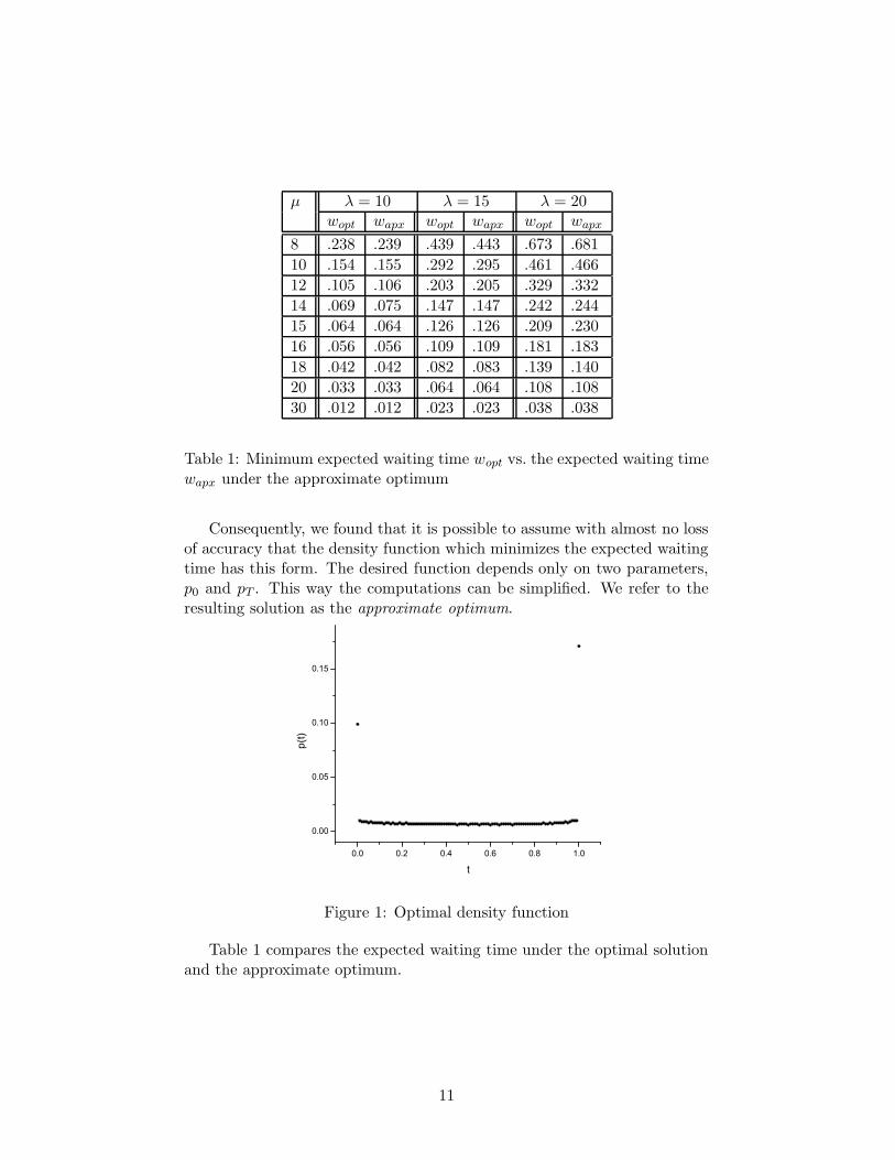
functions obtained have the same property: The density function is approx-imately uniform in (0, T ), and there are positive probabilities p0 and pT , forarrivals at time 0 and T , respectively. For example, in Figure 1 one can seea typical density function. It gives the density function on (0, T ) and alsodepicts the probabilities p0 and pT .

10

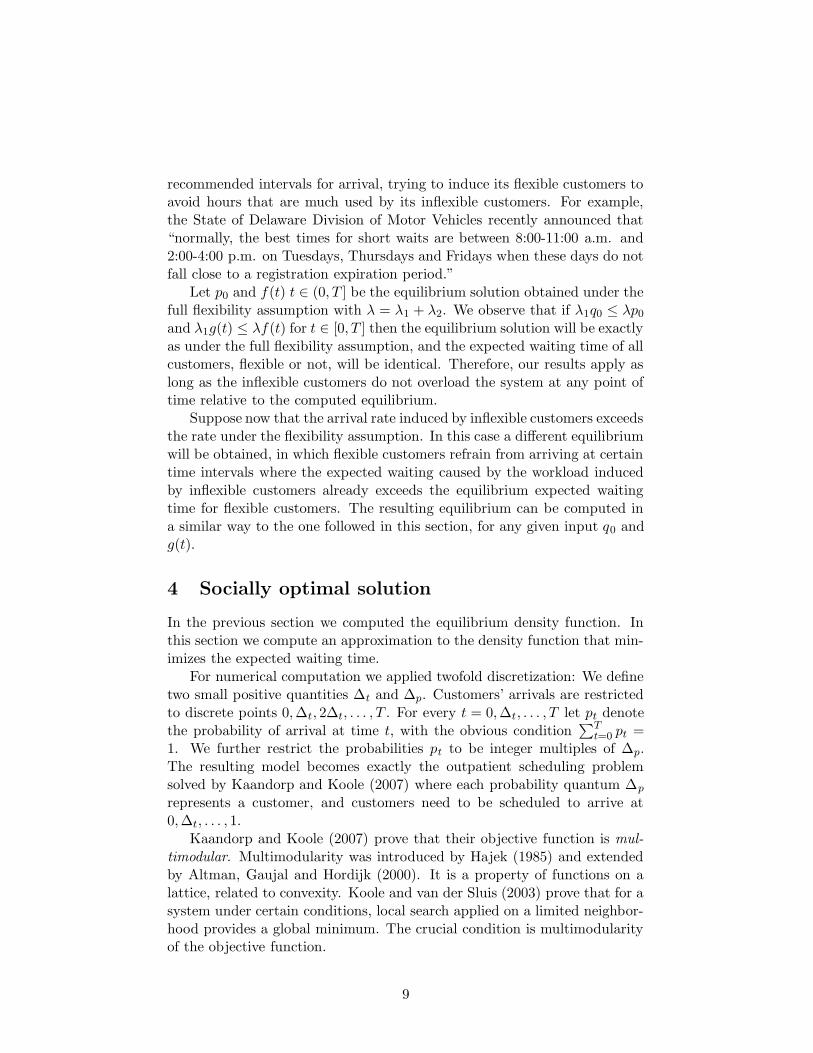
µ λ = 10 λ = 15 λ = 20wopt wapx wopt wapx wopt wapx

8 .238 .239 .439 .443 .673 .681

10 .154 .155 .292 .295 .461 .466

12 .105 .106 .203 .205 .329 .332

14 .069 .075 .147 .147 .242 .244

15 .064 .064 .126 .126 .209 .230

16 .056 .056 .109 .109 .181 .183

18 .042 .042 .082 .083 .139 .140

20 .033 .033 .064 .064 .108 .108

30 .012 .012 .023 .023 .038 .038

Table 1: Minimum expected waiting time wopt vs. the expected waiting timewapx under the approximate optimum

Consequently, we found that it is possible to assume with almost no lossof accuracy that the density function which minimizes the expected waitingtime has this form. The desired function depends only on two parameters,p0 and pT . This way the computations can be simplified. We refer to theresulting solution as the approximate optimum.

Figure 1: Optimal density function

Table 1 compares the expected waiting time under the optimal solutionand the approximate optimum.

11

µ λ = 10 λ = 12 λ = 15 λ = 20

8 .405 .583 .902 1.50010 .238 .348 .562 1.00912 .151 .220 .362 .69114 .101 .146 .241 .47915 .085 .121 .199 .40316 .072 .102 .166 .33618 .053 .074 .119 .24020 .041 .056 .088 .17430 .015 .020 .029 .050

Table 2: Expected waiting time in equilibrium with early arrivals

5 Numerical Results

In this section we present some numerical computations for the models de-scribed above.

We first compute the equilibrium density function with early arrivals,as in Glazer and Hassin (1983). Table 2 presents the equilibrium expectedwaiting time w for various values of λ and µ. Density functions that bringthe system to equilibrium are presented in Figure 2 (left).

Figure 2: Equilibrium density functions with (left) and without (right) earlyarrivals (λ = 10)

12

µ λ = 10 λ = 15 λ = 20w t′ p0 w t′ p0 w t′ p0

8 .397 .43 .635 .895 .92 .955 1.250 - 110 .231 .27 .470 .555 .58 .740 1.000 - 112 .148 .18 .355 .355 .38 .568 .690 .72 .83514 .100 .14 .280 .238 .26 .439 .478 .50 .66915 .083 .11 .249 .198 .23 .396 .399 .43 .60516 .068 .09 .218 .166 .20 .354 .331 .35 .53018 .050 .07 .180 .118 .15 .283 .238 .26 .42820 .039 .06 .156 .088 .12 .235 .170 .19 .34030 .012 .02 .072 .027 .05 .108 .049 .06 .147

Table 3: Equilibrium solutions without early arrivals

µ λ = 10 λ = 15 λ = 20w p0 pT w p0 pT w p0 pT

8 .238 .082 .299 .443 .006 .391 .681 .048 .46410 .154 .082 .248 .294 .006 .337 .466 .051 .41212 .105 .081 .206 .205 .007 .289 .332 .053 .36414 .069 .077 .172 .147 .007 .248 .244 .056 .32115 .064 .075 .158 .126 .007 .230 .210 .057 .30116 .059 .073 .146 .109 .007 .213 .183 .058 .28218 .052 .069 .125 .083 .008 .183 .139 .059 .24820 .033 .064 .108 .064 .008 .157 .108 .060 .21730 .012 .044 .062 .023 .009 .080 .038 .051 .112

Table 4: The approximate optimum

Figure 2 (right) depicts equilibrium density functions and Table 3 presentsthe expected waiting time w for various values of λ and µ when early arrivalsare forbidden. For each µ there are given p0, w, and t′.

Recall from Equation (2) that t′ ≥ w. In Table 3 we compare the valuesof w and t′. Note that when λ is large and µ is small, all customers arriveat the time of opening, i.e., p0 = 1.

Table 4 presents the approximate optimum (p0, pT ), and the correspond-ing value of w for various values of µ and λ.

13

µ λ = 10 λ = 15 λ = 20w1 w2 wapx w1 w2 wapx w1 w2 wapx

8 .405 .397 .239 .902 .895 .443 1.500 1.250 .68110 .238 .231 .154 .562 .555 .294 1.009 1.000 .46612 .151 .148 .105 .362 .355 .205 .691 .690 .33214 .101 .100 .075 .241 .238 .147 .479 .478 .24415 .085 .083 .064 .199 .198 .126 .403 .399 .23016 .072 .068 .056 .166 .166 .109 .336 .331 .18318 .053 .050 .042 .119 .118 .083 .240 .238 .14020 .041 .039 .033 .088 .088 .064 .174 .170 .10830 .015 .012 .012 .029 .027 .023 .050 .049 .038

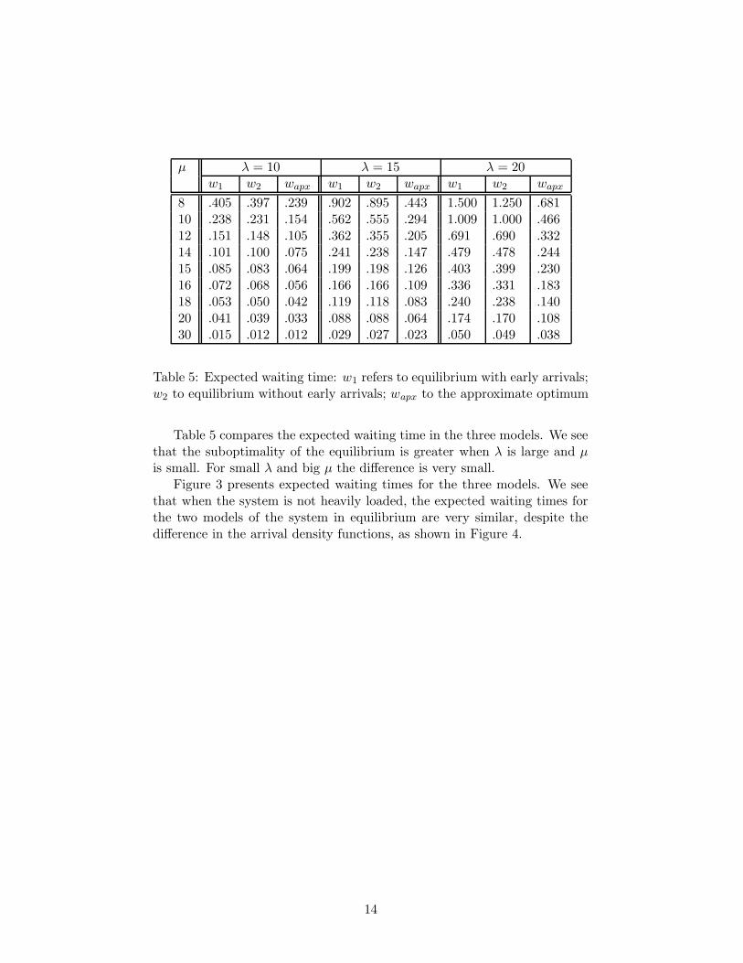
Table 5: Expected waiting time: w1 refers to equilibrium with early arrivals;w2 to equilibrium without early arrivals; wapx to the approximate optimum

Table 5 compares the expected waiting time in the three models. We seethat the suboptimality of the equilibrium is greater when λ is large and µis small. For small λ and big µ the difference is very small.

Figure 3 presents expected waiting times for the three models. We seethat when the system is not heavily loaded, the expected waiting times forthe two models of the system in equilibrium are very similar, despite thedifference in the arrival density functions, as shown in Figure 4.

14

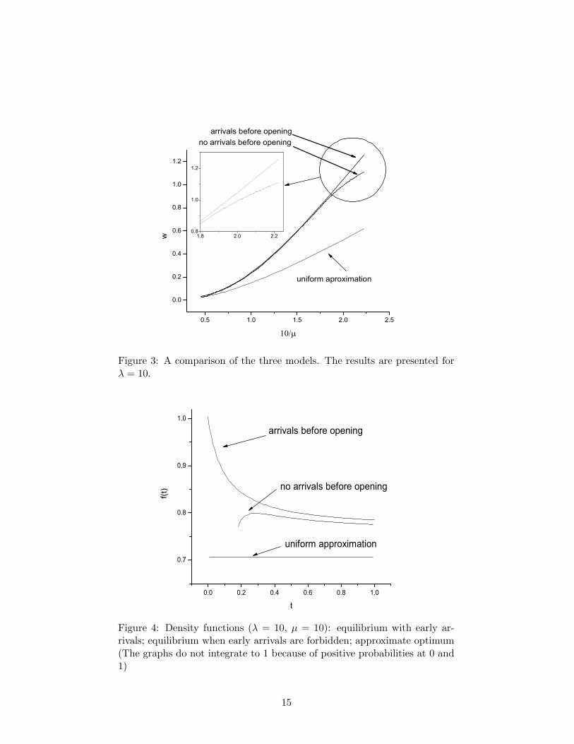
Figure 3: A comparison of the three models. The results are presented forλ = 10.

Figure 4: Density functions (λ = 10, µ = 10): equilibrium with early ar-rivals; equilibrium when early arrivals are forbidden; approximate optimum(The graphs do not integrate to 1 because of positive probabilities at 0 and1)

15

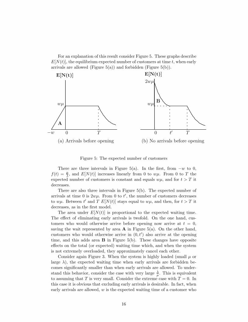
For an explanation of this result consider Figure 5. These graphs describeE[N(t)], the equilibrium expected number of customers at time t, when earlyarrivals are allowed (Figure 5(a)) and forbidden (Figure 5(b)).

wµ wµ

2wµ

0 0T−w Tt′

(a) Arrivals before opening (b) No arrivals before opening

E[N(t)] E[N(t)]

A

B

Figure 5: The expected number of customers

There are three intervals in Figure 5(a). In the first, from −w to 0,f(t) = µ

λ, and E[N(t)] increases linearly from 0 to wµ. From 0 to T the

expected number of customers is constant and equals wµ, and for t > T itdecreases.

There are also three intervals in Figure 5(b). The expected number ofarrivals at time 0 is 2wµ. From 0 to t′, the number of customers decreasesto wµ. Between t′ and T E[N(t)] stays equal to wµ, and then, for t > T itdecreases, as in the first model.

The area under E[N(t)] is proportional to the expected waiting time.The effect of eliminating early arrivals is twofold. On the one hand, cus-tomers who would otherwise arrive before opening now arrive at t = 0,saving the wait represented by area A in Figure 5(a). On the other hand,customers who would otherwise arrive in (0, t′) also arrive at the openingtime, and this adds area B in Figure 5(b). These changes have oppositeeffects on the total (or expected) waiting time which, and when the systemis not extremely overloaded, they approximately cancel each other.

Consider again Figure 3. When the system is highly loaded (small µ orlarge λ), the expected waiting time when early arrivals are forbidden be-comes significantly smaller than when early arrivals are allowed. To under-stand this behavior, consider the case with very large λ

µ. This is equivalent

to assuming that T is very small. Consider the extreme case with T = 0. Inthis case it is obvious that excluding early arrivals is desirable. In fact, whenearly arrivals are allowed, w is the expected waiting time of a customer who

16

arrives at t = 0 and is therefore guaranteed to be the last one. He will waitfor all of the other customers to be served so w = λ

µ. If, on the other hand,

early arrivals are not allowed, all come at time 0 and w = λ2µ

. Thus, in thelimit, excluding early arrivals saves half of the waiting time. However, aswe see from the figure, with λ = 10, excluding early arrivals has almost noeffect for µ > 5. Note that µ ≤ 5 means that the server needs at least twicethe length of time the system is open in order to serve the demand – quitean uncommon situation.

6 Discrete points

We have seen that the expected waiting time of the equilibrium solution,even when early arrivals are forbidden, may be much higher than under anoptimal solution. Clearly, in most cases it is not possible to induce customersto cooperate and behave in the optimal way. In this section we show that byrestricting the time intervals in which the system admits new arrivals, it ispossible to obtain arrival density functions that better resemble the optimalone, and in this way reduce the expected waiting time.

These “degenerate” solutions cannot be part of a first-best socially op-timal solution, but customers do not follow a socially optimal behavior andwe should be satisfied with second-best solutions. It turns out that by re-stricting the arrivals we can obtain better solutions than the unrestrictedequilibrium.

We consider two simple models that are easy to implement.

6.1 Two points

Suppose that we restrict admission to two points of time. The optimal choicefor these points is clearly 0 and T . The question is whether it is possible inthis way to reduce the expected waiting time relative to the original model.

In equilibrium, either all customers arrive at time 0, or the expectedwaiting time of customers arriving at times 0 and T are equal. Considerthe latter case. The expected number of customers arriving at 0 is λp0, andtheir expected waiting time is therefore p0λ

2µ. Denote by R > 0 the expected

remaining time of service after time T , of customers who arrived at time0. Then, taking into account that the expected number of customers whoarrive at T is λ(1−p0), the expected waiting time of a customer who arrives

at T is R + (1−p0)λ2µ

. In equilibrium,

w =p0λ

2µ= R +

(1 − p0)λ

2µ.

Since R > 0,p0λ

2µ>

(1 − p0)λ

2µ=⇒ p0 > 0.5.

17

Table 6 shows some numerical results comparing the equilibrium solu-tions when customers are admitted continuously in [0, T ] (in the two columnsmarked Continuous) and when they are only admitted at 0 and T .

The two-points solution reduces the expected waiting time when thesystem is highly utilized, but not in the extreme cases where p0 = 1 underequilibrium in the continuous model, because in this case we clearly alsoobtain p0 = 1 in the two-points equilibrium.

6.2 Three points

Trying to further reduce the expected waiting time, we allow customer ar-rivals in three discrete points. Clearly, the optimal choice contains 0,T andsome intermediate point which we will choose optimally. Some results arepresented in Table 7. The expected waiting time in this model is clearlyless then in the two-points model, since the two-points model is a specialcase with two of the three points located together. For every three-pointssolution we give the equilibrium expected waiting time w, the probabilitiesp0 and pT of arriving at 0 and T , respectively, and the middle point tm.

Tables 8 and 9 compare the four models: approximately optimal solution,equilibrium when early arrivals are forbidden, arrivals are allowed only attwo points, and arrivals are allowed at three points. As can be seen inTable 8, the arrival probability at the opening time in equilibrium is muchhigher than the desired one. This phenomenon is stronger when the systemis overloaded, with high λ and low µ, and in such cases the gap is narrowedby restricting arrivals the arrivals to two or three points. Table 9 comparesthe resulting expected waiting times.

18

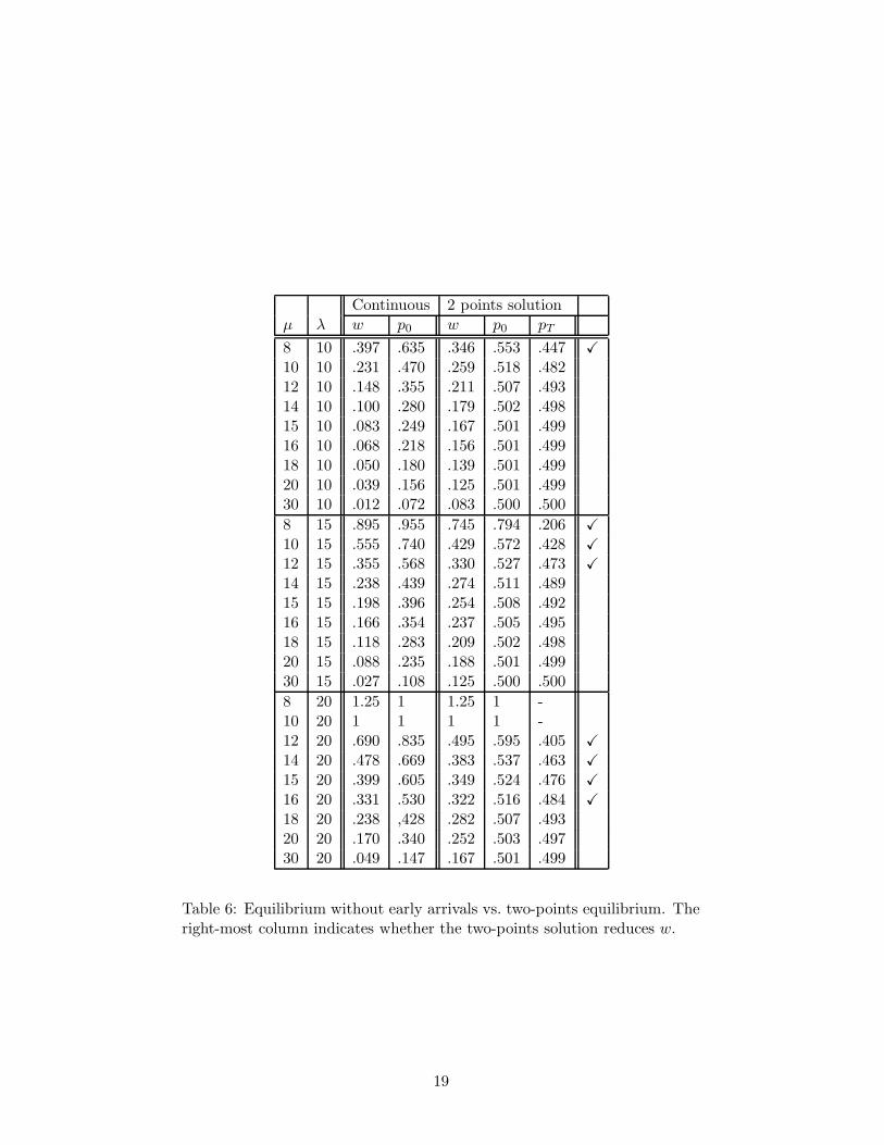
Continuous 2 points solutionµ λ w p0 w p0 pT

8 10 .397 .635 .346 .553 .447 X

10 10 .231 .470 .259 .518 .48212 10 .148 .355 .211 .507 .49314 10 .100 .280 .179 .502 .49815 10 .083 .249 .167 .501 .49916 10 .068 .218 .156 .501 .49918 10 .050 .180 .139 .501 .49920 10 .039 .156 .125 .501 .49930 10 .012 .072 .083 .500 .500

8 15 .895 .955 .745 .794 .206 X

10 15 .555 .740 .429 .572 .428 X

12 15 .355 .568 .330 .527 .473 X

14 15 .238 .439 .274 .511 .48915 15 .198 .396 .254 .508 .49216 15 .166 .354 .237 .505 .49518 15 .118 .283 .209 .502 .49820 15 .088 .235 .188 .501 .49930 15 .027 .108 .125 .500 .500

8 20 1.25 1 1.25 1 -10 20 1 1 1 1 -12 20 .690 .835 .495 .595 .405 X

14 20 .478 .669 .383 .537 .463 X

15 20 .399 .605 .349 .524 .476 X

16 20 .331 .530 .322 .516 .484 X

18 20 .238 ,428 .282 .507 .49320 20 .170 .340 .252 .503 .49730 20 .049 .147 .167 .501 .499

Table 6: Equilibrium without early arrivals vs. two-points equilibrium. Theright-most column indicates whether the two-points solution reduces w.

19

Continuous 3 points solutionµ λ w p0 w p0 tm pT wapx

8 10 .397 .635 .319 .50 .50 .34 .238 X

10 10 .231 .470 .210 .40 .50 .32 .154 X

12 10 .148 .355 .162 .39 .44 .35 .10514 10 .100 .280 .133 .37 .63 .28 .07515 10 .083 .249 .124 .37 .67 .27 .06416 10 .068 .218 .109 .35 .45 .34 .05618 10 .050 .180 .095 .34 .52 .33 .04220 10 .039 .156 .091 .34 .74 .28 .03330 10 .012 .072 .057 .34 .76 .32 .012

8 15 .895 .955 .745 .79 - .21 .443 X

10 15 .555 .740 .429 .57 - .43 .294 X

12 15 .355 .568 .293 .47 .50 .34 .205 X

14 15 .238 .439 .217 .40 .51 .32 .147 X

15 15 .198 .396 .195 .39 .53 .31 .126 X

16 15 .166 .354 .183 .39 .62 .26 .10918 15 .118 .283 .166 .38 .34 .39 .08320 15 .088 .235 .132 .35 .34 .31 .06430 15 .027 .108 .085 .34 .34 .34 .023

8 20 1.25 1 1.25 1 - - .68110 20 1 1 1 1 - - .46612 20 .690 .835 .495 .59 - .41 .332 X

14 20 .478 .669 .357 .50 .53 .34 .244 X

15 20 .399 .605 .312 .47 .50 .35 .210 X

16 20 .331 .530 .306 .49 .38 .45 .183 X

18 20 .238 .428 .221 .40 .48 .34 .139 X

20 20 .170 .340 .185 .37 .52 .32 .10830 20 .049 .147 .114 .34 .63 .32 .038

Table 7: Equilibrium without early arrivals vs. three-points equilibrium.The right-most column indicates whether the three-points solution reducesw.

20

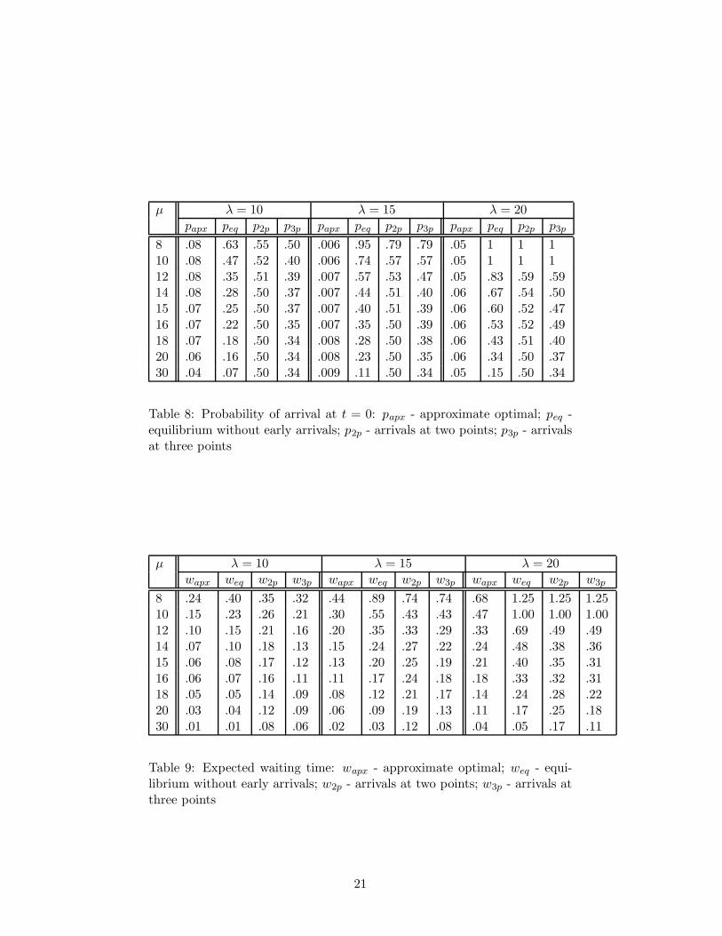
µ λ = 10 λ = 15 λ = 20papx peq p2p p3p papx peq p2p p3p papx peq p2p p3p

8 .08 .63 .55 .50 .006 .95 .79 .79 .05 1 1 110 .08 .47 .52 .40 .006 .74 .57 .57 .05 1 1 112 .08 .35 .51 .39 .007 .57 .53 .47 .05 .83 .59 .5914 .08 .28 .50 .37 .007 .44 .51 .40 .06 .67 .54 .5015 .07 .25 .50 .37 .007 .40 .51 .39 .06 .60 .52 .4716 .07 .22 .50 .35 .007 .35 .50 .39 .06 .53 .52 .4918 .07 .18 .50 .34 .008 .28 .50 .38 .06 .43 .51 .4020 .06 .16 .50 .34 .008 .23 .50 .35 .06 .34 .50 .3730 .04 .07 .50 .34 .009 .11 .50 .34 .05 .15 .50 .34

Table 8: Probability of arrival at t = 0: papx - approximate optimal; peq -equilibrium without early arrivals; p2p - arrivals at two points; p3p - arrivalsat three points

µ λ = 10 λ = 15 λ = 20wapx weq w2p w3p wapx weq w2p w3p wapx weq w2p w3p

8 .24 .40 .35 .32 .44 .89 .74 .74 .68 1.25 1.25 1.2510 .15 .23 .26 .21 .30 .55 .43 .43 .47 1.00 1.00 1.0012 .10 .15 .21 .16 .20 .35 .33 .29 .33 .69 .49 .4914 .07 .10 .18 .13 .15 .24 .27 .22 .24 .48 .38 .3615 .06 .08 .17 .12 .13 .20 .25 .19 .21 .40 .35 .3116 .06 .07 .16 .11 .11 .17 .24 .18 .18 .33 .32 .3118 .05 .05 .14 .09 .08 .12 .21 .17 .14 .24 .28 .2220 .03 .04 .12 .09 .06 .09 .19 .13 .11 .17 .25 .1830 .01 .01 .08 .06 .02 .03 .12 .08 .04 .05 .17 .11

Table 9: Expected waiting time: wapx - approximate optimal; weq - equi-librium without early arrivals; w2p - arrivals at two points; w3p - arrivals atthree points

21

7 Concluding remarks

This paper considers a non-stationary queueing model with opening andclosing times. We characterize the equilibrium solution and describe theunderlying equations that govern it. Since an analytical solution of thismodel is out of reach, we solve it numerically. Our model is a variation ofthe one solved by Glazer and Hassin (1983), and it is motivated by naturalquestions concerning the ability to reduce the waiting time of customers whoact independently and aim to maximize their individual welfare. This line ofresearch falls within the growing research on strategic behavior in queueingsystems.

We show that excluding early arrivals doesn’t yield a significant reduc-tion in expected waiting time unless the system is very heavily loaded (i.e.,it is open for a short time relative to the demand).

The optimal strategy can be approximated fairly well by uniform dis-tribution in the open interval (0, T ) and positive probabilities p0 and pT ,representing the probabilities for a customer to arrive at time 0 and T respec-tively. Such approximate solution can be characterized by two parametersonly. We compare an approximate optimal solution with the equilibriumsolutions. The ratio between the expected waiting time under equilibriumand under the optimal solution increases when the system becomes moreheavily loaded.

Finally, we computed the expected waiting time in equilibrium whenarrivals are restricted to time 0 or T , and when they are in addition allowedat one internal point. Improved results are obtained by these restrictionsof the arrival instants when the system is heavily loaded. In these cases,when the system is open continuously in [0, T ], too many customers tend toarrive at t = 0 ignoring the effect their arrival has on those who arrive later.The two and three-points restrictions reduce the probability that a customerarrives at the opening instant and by this reduce the expected waiting time.

A nice feature of these results is the simplicity of their implementation, incontrast, for example, to the common way of controlling customers behaviorthrough price mechanisms. In our case, such a mechanism could be a time-dependent entry fee that seems quite impractical. We leave the questionof whether other practical alternatives exist for future research. Anotherquestion for future research is whether restricting arrival times to smallsets can be useful in reducing customers’ waiting time in other models, forexample in the scheduled batch service considered by Glazer and Hassin(1987).

References

[1] E. Altman, B. Gaujal, and A. Hordijk, “Multimodularity, convexity, andoptimization properties,” Mathematics of Operations Research 25 324-347

22

(2000).

[2] M. Arbatskaya, K. Mukhopadhaya, and E. Rasmusen, “The Parking LotProblem,” Indiana University, Kelley School of Business, Department of Busi-ness Economics and Public Policy (2007).

[3] R. Arnott, A. de Palma, and R. Lindsey, “Information and time-of-usagedecisions in the bottleneck model with stochastic capacity and demand,”European Economic Review 43 525-548 (1999).

[4] N. J. Bearden, A. Rapoport, and D. A. Seale, “Entry times in queues withendogenous arrivals: Dynamics of play on the individual and aggregate lev-els,” Experimental Business Research (A. Rapoport and R. Zwick Eds.) 55

201-221 (2005).

[5] T. Cayirli and E. Veral, “Outpatient scheduling in health care: a review ofliterature,” Production and Operations Management 12 519-549 (2003).

[6] A. Glazer and R. Hassin, “?/M/1: on the equilibrium distribution of customerarrivals,” European Journal of Operational Research 13 146-153 (1983).

[7] A. Glazer and R. Hassin, “Equilibrium arrivals in queues with bulk serviceat scheduled times,” Transportation Science 21 273-278 (1987).

[8] P. Guo, J.J. Liu, and Y. Wang, “Intertemporal service pricing with strategiccustomers,” Operations Research Letters 37 420-424 (2009).

[9] B. Hajek, “Extremal splittings of point processes,” Mathematics of Opera-

tions Research 10 543-556 (1985).

[10] R. Hassin and M. Haviv, To Queue Or Not To Queue: Equilibrium Behavior

in Queueing Systems Kluwer (2003).

[11] M. Hlynka, “Real Life Queueing Examples,”http://www2.uwidsor.ca/ hlynka/qreal.html, (1985).

[12] G. Kaandorp and G. Koole, “Optimal outpatient appointment scheduling,”Health Care Management Science 10, 217-229 (2007).

[13] G. Koole and E. van der Sluis, “Optimal shift scheduling with global servicelevel constraint,” IIE Transactions 35 1049-1055 (2003).

[14] B. Jansson, “Choosing a good appointment system—A study of queues of thetype (D/M/1),” Operations Research 14 292-312 (1966).

[15] A. Lago and C. F. Daganzo, “Spillovers, merging traffic and the morningcommute,” Transportation Research Part B 41 670-683 (2007).

[16] M. A. Lariviere and J. A. van Mieghem, “Strategically seeking service: howcompetition can generate Poisson arrival,” Manufacturing & Service Opera-

tions Management 6 23-40 (2004).

[17] V. V. Mazalov and J. V. Chuiko, “Nash Equilibrium in the Optimal Arrivaltime problem,” Computational Technologies 11 60-71 (2006). In Russian.

[18] M. Ostrovsky and M. Schwarz, “Adoption of standards under uncertainty,”The Rand Journal of Economics 36 816-832 (2005).

23

[19] M. Ostrovsky and M. Schwarz, “Synchronization under uncertainty,” Inter-

national Journal of Economic Theory 2 1-16 (2006).

[20] H. Ostubo and A. Rapoport, “Vickrey’s model of traffic congestion dis-cretized,” Transportation Research Part B: Methodological 42 873-889 (2008).

[21] A. Rapoport, W. E. Stein, J. E. Parco and D. A. Seale, “Equilibrium play insingle-server queues with endogenously determined arrival times,” Journal of

Economic Behaviour & Organization 55 67-91 (2004).

[22] D. A. Seale, J. E. Parco, W. E. Stein, and A. Rapoport, “Joining a queue orstaying out: Effect of information structure and service time on arrival andstaying out decisions,” Experimental Economics 8 117-144 (2005).

[23] W.S. Vickrey, “Congestion theory and transport investment,” The American

Economic Review 59 251-260 (1969).

[24] S. Wang and L. Zhu, “A dynamic queuing model,” The Chinese Journal of

Economic Theory 1 14-35 (2004).

Refael Hassin is a professor of Operations Research at Tel Aviv Uni-versity, specializing in Combinatorial Optimization and Queueing modelsinvolving strategic behavior of customers and servers.

Yana Kleiner is a software engineer at Intel Israel. She holds a B.Scdegree in Information Systems from the Technion - Israel Institute of Tech-nology, and M.Sc. degree in Operations Research from Tel Aviv University.

24