equilibrium competition, social welfare and corruption in
TRANSCRIPT
Social Choice and Welfare (2019) 53:443–465https://doi.org/10.1007/s00355-019-01192-8
ORIG INAL PAPER
Equilibrium competition, social welfare and corruptionin procurement auctions
Minbo Xu1 · Daniel Z. Li2
Received: 16 September 2018 / Accepted: 30 April 2019 / Published online: 11 May 2019© The Author(s) 2019
AbstractWe study the effects of corruption on equilibrium competition and social welfare in apublic procurement auction. A government pays costs to invite firms to the auction,and a bureaucrat who runs the auction may request a bribe from the winning firm. Wefirst show that, with no corruption, the bureaucrat will invite more than the sociallyoptimal number of firms to the auction. Second, the effects of corruption on equilibriumoutcomes vary across different forms of bribery. For a fixed bribe, corruption does notaffect equilibriumcompetition, yet it does induce socialwelfare loss. For a proportionalbribe, the bureaucrat may invite either fewer or more firms, depending on how muchhe weights his private interest relative to the government payoff. Finally, we show thatinformation disclosure may consistently induce more firms to be invited, regardlessof whether there is corruption.
1 Introduction
Public procurements account for a substantial part of economies worldwide. In theEuropeanUnion (EU),more than 250,000 public authorities spend approximately 14%of GDP on the purchase of services and supplies each year.1 Naturally, corruption is acommon concern in public procurements. To prevent corruption,most countries imple-ment laws and regulations to guarantee the necessary competition and transparency inpublic procurements. For instance, the EU requires a minimum of 35 days for a publiccontract notice in an open procedure, for which any business can submit a bid; and in a
1 EU website, http://ec.europa.eu/growth/single-market/public-procurement/index_en.htm.
B Daniel Z. [email protected]
Minbo [email protected]
1 Business School, Beijing Normal University, Beijing, China
2 Department of Economics and Finance, Durham University Business School, Mill Hill Lane, DurhamDH1 3LB, UK
123
444 M. Xu, D. Z. Li
restricted procedure, for which only those who are pre-screened are invited to submita bid, a public authority must invite at least 5 bidders to the competition process.2
The belief underlying these rules is that competition may help improve efficiency andreduce corruption.
The literature has mainly focused on the effects of competition on corruption,yet has paid relatively less attention to the reverse causality between them. In thispaper, we provide a theoretical investigation of the effects of corruption on equilibriumcompetition and social welfare in a public procurement auction. Specifically, in ourmodel, there is a government agent, such as the Department of Defense, a bureaucratwho runs the auction on behalf of the government, and a number of potential firmswho can submit bids for the government contract if invited. The government needsto pay costs to screen and invite firms to participate, and the corrupt bureaucrat mayrequest a bribe from the winning firm.3
We consider a standard first-price procurement auction, which is common in prac-tice.4 In the auction, the firm with the lowest production cost wins, and the pricereceived by the firm is equal to its bid. Given the value of the contract, the govern-ment’s objective is tominimize the government spending, e.g., the sumof the invitationcosts and the price paid to the winning firm. The bureaucrat, if corrupt, cares about aweighted average of the bribe received by him and the government payoff; if honest,his objective is in line with that of the government.
In the absence of corruption, we first show that the bureaucrat will invite more thanthe socially optimal number of firms to the auction, under the standard assumptions thatfirms’ cost distribution is of decreasing reversed hazard rate (DRHR) and that there isa positive invitation cost.5 In other words, the optimal number of firms that maximizesthe government’s payoff is larger than the efficient number of firms that maximizessocial welfare. This over-invitation result is not surprising as the government is notmodeled as a social planner in our model. The intuition behind the result is thatinviting an extra firm reduces the expected total surplus of the firms, due to increasedcompetition, which is ignored by the payoff-maximizing government but is taken intoaccount in the total social welfare.
We then introduce corruption into the model, in which the bureaucrat requests abribe from the winning firm of the auction.We consider two common forms of bribery.The first is a fixed bribe inwhich the bureaucrat requests thewinning firm to pay a fixedamount as a bribe. For instance, the fixed bribe can be in the form of a commissionfee or a kickback that is common in the real world (Inderst and Ottaviani 2012). Thesecond is a proportional bribe, whereby the winning firm must share a proportion ofits revenue with the corrupt bureaucrat (Acemoglu and Verdier 2000; Amir and Burr
2 See http://europa.eu/youreurope/business/public-tenders/rules-procedures/index_en.htm. Updated inSep. 2018.3 This practice apprears in all public sectors, and a portion of the sum that a winning contractor receivedis designated for the official as kickbacks. See the report prepared for the European Commission by PwCand Ecorys, “Identifying and Reducing Corruption in Public Procurement in the EU.” June 30, 2013.4 We also consider the format of second-price procurement auctions in this paper, and show that mainresults of our paper are robust in both formats of auctions.5 If there is no invitation cost, Compte and Jehiel (2002) show that the participation of an extra bidderalways increases the social welfare in procurement auctions with symmetric competitors.
123
Equilibrium competition, social welfare and corruption… 445
2015). For example, in Indonesia, the former president Suharto was publicly knownas “Mr. Twenty-Five Percent” because he required that all major contracts throughoutthe nation give him 25% of the income.6
Our main result is that the effects of corruption on equilibrium competition andsocial welfare vary across different forms of bribery.When the bribe is a fixed amount,the corrupt bureaucrat invites the same number of firms as in the absence of corruption,as his marginal incentive of inviting firms remains the same as before. Therefore,corruption in this form does not affect equilibrium competition. However, it doeschange social welfare and resource allocation in equilibrium. We show that, under theexpectation of paying a fixed bribe upon winning, all firms will mark up their bids bythe same amount, which in turn increases the expected payment of the government tothe winning firm. As a result, the fixed bribe is paid by the government, and it does nothurt the firms at all. The increased public expenditure by the government then implieswelfare loss due to the marginal cost of distortion of public funds.
By contrast, under a proportional bribe, the corrupt bureaucrat may invite eitherfewer or more firms to the auction, depending on how much the bureaucrat weightshis personal interest relative to the government payoff. We first show that, in this case,firms will adjust their bids proportionally in equilibrium. Second, there are two oppo-site effects on the equilibrium competition. On the one hand, as firms’ bids increaseproportionally, the distribution of the bids becomes more dispersed, which decreasescompetition in the auction. In response to it, the bureaucrat needs to encourage com-petition by inviting more firms. On the other hand, the bureaucrat also has an incentiveto discourage competition, as the winning firm’s revenue is decreasing in the numberof firms in the auction. The relative magnitude between these two opposite effectsdetermines the equilibrium level of competition.
We further investigate the effects of government information disclosure on auc-tion outcomes. When firms’ areas of specialization are differentiated, revealing moreproject information by the government may induce a more dispersed distribution offirms’ cost estimates. For example, information disclosure may drive up the cost esti-mates of some firms that find it is a mismatch to their areas of specialization, whiledriving down those of others that find it to be a good match. As a result, firms’ costestimates becomemore dispersed.We show that information disclosure increases boththe efficient and the optimal number of firms in procurement auctions. The intuition isthat under information disclosure, firms’ cost estimates become more dispersed, andthe auction becomes less competitive than before. It is then better to invite more firmsto participate in the auction.
Finally, we also explore the policy implications of our results. For the regulation ofpublic procurements, we show that imposing a requirement on the minimum numberof bidders may be effective only when it lies in a reasonable range. For instance, if itis too low, it will not impose real restrictions on a corrupt bureaucrat’s choice; if it istoo high, it may instead cause a welfare loss.
Motivated by Rose-Ackerman (1978)’s argument that increasing in competitionhelps reduce corruption, there is a strand of literature studying the effects of competi-
6 Wrage, Alexandra Addison. Bribery and Extortion: Undermining Business, Governments, and Security.Westport, Conn.: Praeger Security International, 2007. p. 14.
123
446 M. Xu, D. Z. Li
tion on corruption in a large variety of economic contexts, and the results suggest thatthe relationship is complicated. For example, Shleifer and Vishny (1993) and Blissand Di Tella (1997) show that the effect of competition on corruption depends on thenature of corruption. In the empirical studies, Ades and Di Tella (1999) and Emerson(2006) find that market competition and corruption are negatively related, while Alex-eev and Song (2013) find a positive relationship between the strength of competitionand the extent of corruption. The existing literature has paid relatively less attentionto the effects of corruption on competition, though its empirical importance has beenemphasized. One exception is Amir and Burr (2015), who examine theoretically theeffects of corruption in the entry-certifying process on market structure and socialwelfare for a Cournot industry.
Our paper joins a small but growing literature that restricts attention to corruptionin public procurements.7 Specifically, two papers examine the relationship betweencompetition and corruption in procurement. Celentani and Ganuza (2002) study theimpact of the number of potential suppliers on equilibrium corruption in the agencymodel and find that corruption may be higher in a more competitive environment.Compte et al. (2005) analyze the effect of corruption on price competition in whichthe corrupt bureaucrat may offer a firm an opportunity to readjust its bid and firmscompete for this favor by making bribe offers. In this paper, we investigate the effectsof various forms of bribery on the number of invited firms and social welfare inprocurement auctions.
In the context of auctions, corruption is commonly described as an act in which abureaucrat manipulates the auction rules in exchange for bribes. For example, Compteet al. (2005) and Menezes and Monteiro (2006) consider a corruption model in whichthe bureaucrat may offer a favored firm an opportunity to readjust its initial bid inexchange for a bribe. Other related papers include Burguet and Perry (2009) andArozamena andWeinschelbaum (2009). Another strand of literature studies corruptionin multidimensional procurement auctions, whereby the government may care aboutboth the price and quality of the project. Celentani and Ganuza (1999, 2002) andBurguet and Che (2004) examine corruption in which the bureaucrat manipulatesthe quality assessment to favor the firms offering higher bribes. In our paper, theauction rule is taken as given, yet the bureaucrat may endogenously determine thecompetition level in the auction. Specifically, the bribery studied in our paper is aform of “harassment bribe” (Basu 2011), inwhich the bribe is exchanged for deliveringentitled services rather than undue favors.
Our paper is also related to the literature on auctions with participation costs.The participation costs can be either paid by the bidders (McAfee and McMillan1987; Levin and Smith 1994), or by the auctioneer (Szech 2011; Li 2017; Lee andLi 2018). The benchmark setting of our model is closely related to Szech (2011).Though different from her model of ascending second-price auction, we study a first-price procurement auction, yet the extension is straightforward according to standard
7 For example, Burguet and Che (2004) examine the inefficiency cost of bribery in scoring procurement;Auriol (2006) compares capture to extortion in public purchase; Lengwiler and Wolfstetter (2006) reviewsome forms of corruption; Arozamena andWeinschelbaum (2009) analyze effects of a right-of-first-refusalclause in first-price auctions; Burguet (2017) designs the optimal procurement mechanism in the presenceof corruption.
123
Equilibrium competition, social welfare and corruption… 447
auction theory. The key differences in our model are twofold: first, we consider apublic procurement auction with a broader definition of social welfare, which takesSzech (2011) as a special case; second, the focus of our paper is on the effects ofcorruption on equilibrium bidding strategy, competition and social welfare in a publicprocurement auction.
The remainder of this paper is organized as follows. Section 2 introduces thebenchmark model of procurement auction with no corruption. Section 3 studies theequilibrium outcomes under corruption, and there are two cases, the fixed bribe andproportional bribe. Section 4 provides some further discussions, and Sect. 5 presentsour concluding remarks.
2 Benchmark: no corruption
Consider a public procurement auction in which a government plans to allocate anindivisible contract among a number of firms. A bureaucrat runs the auction on behalfof the government. We assume there are a large number of potential firms qualified forthis contract, and n firms are invited to the auction at a cost of C(n), which is paid bythe government. The value of the contract to the government is V . The cost functionC(n) is increasing and weakly convex, that is, C ′(n) > 0 and C ′′(n) ≥ 0. The firmsare ex ante homogenous whose production cost X conforms to the distribution of F(·)on [0, V ], with strictly positive density f (·). Assume all players are risk-neutral.
For those invited firms, let {Xi }ni=1 be n independent draws from the same distri-bution F(·), where Xi is the production cost for firm i . The distribution of F (·) iscommon knowledge, yet the realization of Xi is only observed by firm i . Let X (k)
ndenote the kth lowest cost of the n invited firms and
X (1)n ≤ X (2)
n ≤ · · · ≤ X (n)n .
Let F (k)n (·) and f (k)
n (·) be the cumulative distribution function and probability densityfunction of X (k)
n .We consider a sealed-bid first-price procurement auction, which is common in
practice. It is well known that the symmetric equilibrium bidding strategy in a first-price procurement auction is given by (e.g., Krishna 2002, p.17),
b(x) = E[X (1)n−1|X (1)
n−1 > x]
= x +∫ V
x
F̄ (1)n−1(y)
F̄ (1)n−1(x)
dy,
where F̄ (1)n−1(x) = 1− F (1)
n−1(x) is the survival function. The firm with the lowest cost
X (1)n wins, and its revenue is equal to its bid b(X (1)
n ). The rent for the winning firm isthus
R(n) = b(X (1)n ) − X (1)
n . (1)
123

448 M. Xu, D. Z. Li
The government’s payoff is equal to the net project benefit minus the invitationcost, which is
�(n) = V − b(X (1)n ) − C(n). (2)
It is worth noting that we do not model the government as a social planner. Instead, wemodel it as a government agency that cares about its own payoff rather than the overallsocial welfare. For example, the Department of Defense in the U.S. procures weaponssystems, and its primary concerns are the budget spending and the performance of theweapons system procured.
We next consider the social welfare. Government spending is financed throughtaxation, which includes the payment to the winning firm, b(X (1)
n ), and the invitationcost C(n). We assume there is a marginal cost of public funds, λ ∈ [0, 1), due to theallocative distortion caused by taxation (Laffont and Tirole 1987). The social welfareW (n) is thenmeasured by the sum of the firms’ winning rent in (1) and the governmentpayoff in (2), minus the distortion cost of public funds, that is
W (n) = V − X (1)n − λb(X (1)
n ) − (1 + λ)C(n). (3)
By introducing λ, the marginal cost of public funds, into our model of public procure-ments, we provide a broader definition of social welfare than that in standard auctionliterature, e.g., Szech (2011), which corresponds to the special case of λ = 0 in ourmodel.
TheRevenueEquivalence Theorem shows that the expected payment to thewinningfirm is equal to the expected second-lowest production cost, that is, E[b(X (1)
n )] =E[X (2)
n ]. To further characterize the properties of E[X (1)n ] and E[X (2)
n ], we make thefollowing standard assumption in procurement auctions, that the distribution of Xsatisfies the property of decreasing reversed hazard rate.
Definition 1 The distribution of X is of decreasing reversed hazard rate (DRHR) if itsreversed hazard rate of f (x)/F(x) is decreasing in x .
The DRHR assumption in the procurement auction is analogous to the regularitycondition of increasing failure rate in the standard ascending price auction (Myerson1981). The difference is that in a procurement auction, the bidder offering the lowestbid wins the auction, whereas in a standard ascending price auction the bidder offeringthe highest bid wins. There are many examples of DRHR distributions, such as uni-form, truncated normal and exponential distributions. Lemma 1 below provides someproperties of E[X (1)
n ] and E[X (2)n ].
Lemma 1 (i) E[X (1)n ] is strictly decreasing and strictly convex in n, and limn→∞
E[X (1)n ] = 0.
(ii) If the distribution of X is of DRHR, then E[X (2)n ] is strictly decreasing and strictly
convex in n, and limn→∞ E[X (2)n − X (2)
n+1] = 0.
(iii) If the distribution of X is of DRHR, then E[R(n)] = E[X (2)n − X (1)
n ] is strictlydecreasing and strictly convex in n, and limn→∞ E[R(n)] = 0.
Proof Please refer to the Appendix for all the omitted proofs in this paper. �
123

Equilibrium competition, social welfare and corruption… 449
Lemma 1 is analogous to Lemma 1–4 in Szech (2011).8 The monotonicity propertyof E[X (1)
n ] is straightforward as X (1)n is the smallest order statistic. As n increases,
E[X (1)n ] will naturally decrease and converge to zero. The similar property holds for
E[X (2)n ] under the assumption of DRHR. If the distribution of X is of DRHR, we have
the result that the expected rent of the winning firm will gradually squeeze out as thenumber of firms increases. A direct implication of Lemma 1 is that
E[X (2)n − X (2)
n+1
]> E
[X (1)n − X (1)
n+1
], (4)
that is, if one more firm joins the auction, the expected value of E[X (2)n ] drops faster
than E[X (1)n ].
The bureaucrat runs the auction on behalf of the government, and he decides howmany firms to invite. In the absence of corruption, the bureaucrat just chooses theoptimal number of firms, denoted by n∗, that maximizes the expected payoff of thegovernment. We are also interested in social welfare and denote n∗∗ as the efficientnumber of firms that maximizes the expected social welfare. By definition,
n∗ = argmaxn
E[�(n)] and n∗∗ = argmaxn
E[W (n)].
The results in Lemma 1 imply that both E[�(n)] and E[W (n)] are concave in n underthe DRHR assumption, and therefore, both n∗ and n∗∗ are well-defined and finite. Ourfirst result is that, when there is no corruption, the bureaucrat will invite more than thesocially optimal number of firms to the auction.
Proposition 1 If the distribution of X is of DRHR, then
n∗ ≥ n∗∗. (5)
The over-invitation result is not surprising, and a similar result is also reported inSzech (2011, Proposition 1) in a model of ascending second-price auction. Here, weinstead study a descending first-price auction, and more importantly, we explicitlyconsider the distortion cost of public funds and provide a more general definition ofsocial welfare, which takes Szech’s model as a special case of λ = 0. Therefore,Proposition 1 provides a non-trivial extension of the results in the literature.
We would like expatiate a little more on the insights of the over-invitation result.For increasing n, the marginal change in the expected government payoff is
�E[�(n)] = E[X (2)n − X (2)
n+1
]− (C(n + 1) − C(n)),
and we can normalize the marginal change of the expected social welfare as
1
1 + λ�E[W (n)] = 1
1 + λE
[X (1)n − X (1)
n+1
]+ λ
1 + λE
[X (2)n − X (2)
n+1
]− (C(n + 1) − C(n)).
8 The difference is that Szech (2011) studied an ascending second-price auction, while we consider adescending first-price procurement auction and derive the results based on the different distribution assump-tion of DRHR.
123

450 M. Xu, D. Z. Li
O n
11+λ
ΔE[W (n)]
ΔE[Π(n)]
n∗n∗∗
Fig. 1 Over-invitation Result: When there is no corruption and a positive invitation cost, the bureaucrat willinvite more than the socially optimal number of firms to the auction
Inequality (4) then implies that �E[�(n)] is greater than 11+λ
�E[W (n)]. That is, forany given n, the marginal government payoff is greater than the normalized marginalsocial welfare, and therefore, the expected government payoff approaches its maxi-mum more slowly than the expected social welfare. The economic intuition is that,when n increases, the expected winning rent of the firms decreases, which is ignoredby the government but is taken into account in the total social welfare. Figure 1 belowillustrates the result of over-invitation.
We next provide a simple example where X conforms to a uniform distribution,that may help illustrate the over-invitation result.
Example 1 Let X ∼ U [0, V ], and C(n) = nc, where c is constant. The distributionfunctions of X (1)
n and X (2)n are given in (12) in the Appendix, and it follows that
E[X (1)n ] = V
n+1 and E[X (2)n ] = 2V
n+1 .With no corruption, the bureaucrat chooses n to maximize the government’s
expected payoff,
maxn
E[�(n)] = V − E[X (2)n ] − nc = V − 2
n + 1V − nc.
The marginal government payoff is �E[�(n)] = 2V(n+1)(n+2) − c, and the optimal
condition for n∗ is
n∗(n∗ + 1) ≤ 2V
c< (n∗ + 1)(n∗ + 2).
We next solve the problem of maximizing the expected social welfare:
maxn
E[W (n)] = V − E[X (1)n ] − λE[X (2)
n ] − (1 + λ)nc.
123
Equilibrium competition, social welfare and corruption… 451
The normalized marginal change in social welfare is
1
1 + λ�E[W (n)]= 1
1 + λ· V
(n + 1)(n + 2)+ λ
1 + λ· 2V
(n + 1)(n + 2)−c<�E[�(n)].
The optimal condition for n∗∗ is thus
n∗∗(n∗∗ + 1) ≤ (1 + 2λ)V
(1 + λ)c< (n∗∗ + 1)(n∗∗ + 2).
It follows that, n∗ ≥ n∗∗, as 1+2λ1+λ
≤ 2. For example, if λ = 0.2, c = 2 and V = 36,then we have n∗ = 5 and n∗∗ = 4. This result confirms the over-invitation result of(5) in Proposition 1.
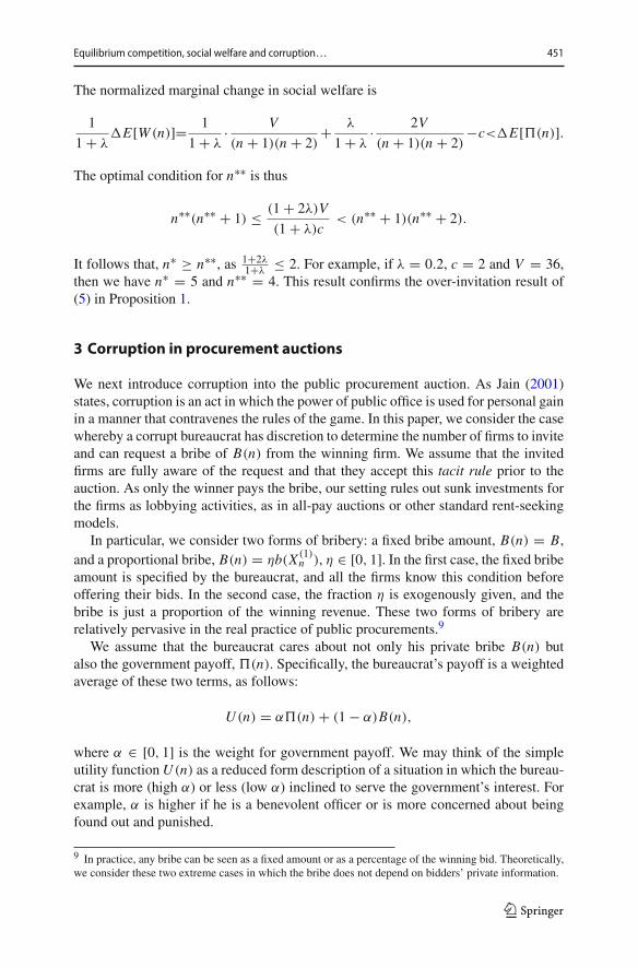
3 Corruption in procurement auctions
We next introduce corruption into the public procurement auction. As Jain (2001)states, corruption is an act in which the power of public office is used for personal gainin a manner that contravenes the rules of the game. In this paper, we consider the casewhereby a corrupt bureaucrat has discretion to determine the number of firms to inviteand can request a bribe of B(n) from the winning firm. We assume that the invitedfirms are fully aware of the request and that they accept this tacit rule prior to theauction. As only the winner pays the bribe, our setting rules out sunk investments forthe firms as lobbying activities, as in all-pay auctions or other standard rent-seekingmodels.
In particular, we consider two forms of bribery: a fixed bribe amount, B(n) = B,and a proportional bribe, B(n) = ηb(X (1)
n ), η ∈ [0, 1]. In the first case, the fixed bribeamount is specified by the bureaucrat, and all the firms know this condition beforeoffering their bids. In the second case, the fraction η is exogenously given, and thebribe is just a proportion of the winning revenue. These two forms of bribery arerelatively pervasive in the real practice of public procurements.9
We assume that the bureaucrat cares about not only his private bribe B(n) butalso the government payoff, �(n). Specifically, the bureaucrat’s payoff is a weightedaverage of these two terms, as follows:
U (n) = α�(n) + (1 − α)B(n),
where α ∈ [0, 1] is the weight for government payoff. We may think of the simpleutility functionU (n) as a reduced form description of a situation in which the bureau-crat is more (high α) or less (low α) inclined to serve the government’s interest. Forexample, α is higher if he is a benevolent officer or is more concerned about beingfound out and punished.
9 In practice, any bribe can be seen as a fixed amount or as a percentage of the winning bid. Theoretically,we consider these two extreme cases in which the bribe does not depend on bidders’ private information.
123
452 M. Xu, D. Z. Li
We do not consider a penalty for corruption if detected, although it could be intro-duced in a straightforward way, for example, a detecting probability that is decreasingin α and a penalty that is proportional to B(n). Our main focus here is on the effects ofcorruption on equilibrium competition and social welfare in the procurement auction.The introduction of a penalty will at most temper but will not change the direction ofthe results; therefore, we avoid that complication in our model.
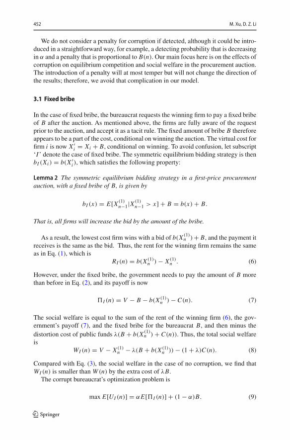
3.1 Fixed bribe
In the case of fixed bribe, the bureaucrat requests the winning firm to pay a fixed bribeof B after the auction. As mentioned above, the firms are fully aware of the requestprior to the auction, and accept it as a tacit rule. The fixed amount of bribe B thereforeappears to be a part of the cost, conditional on winning the auction. The virtual cost forfirm i is now X ′
i = Xi + B, conditional on winning. To avoid confusion, let subscript‘I ’ denote the case of fixed bribe. The symmetric equilibrium bidding strategy is thenbI (Xi ) = b(X ′
i ), which satisfies the following property:
Lemma 2 The symmetric equilibrium bidding strategy in a first-price procurementauction, with a fixed bribe of B, is given by
bI (x) = E[X (1)n−1|X (1)
n−1 > x] + B = b(x) + B.
That is, all firms will increase the bid by the amount of the bribe.
As a result, the lowest cost firm wins with a bid of b(X (1)n )+ B, and the payment it
receives is the same as the bid. Thus, the rent for the winning firm remains the sameas in Eq. (1), which is
RI (n) = b(X (1)n ) − X (1)
n . (6)
However, under the fixed bribe, the government needs to pay the amount of B morethan before in Eq. (2), and its payoff is now
�I (n) = V − B − b(X (1)n ) − C(n). (7)
The social welfare is equal to the sum of the rent of the winning firm (6), the gov-ernment’s payoff (7), and the fixed bribe for the bureaucrat B, and then minus thedistortion cost of public funds λ(B + b(X (1)
n ) + C(n)). Thus, the total social welfareis
WI (n) = V − X (1)n − λ(B + b(X (1)
n )) − (1 + λ)C(n). (8)
Compared with Eq. (3), the social welfare in the case of no corruption, we find thatWI (n) is smaller than W (n) by the extra cost of λB.
The corrupt bureaucrat’s optimization problem is
max E[UI (n)] = αE[�I (n)] + (1 − α)B. (9)
123
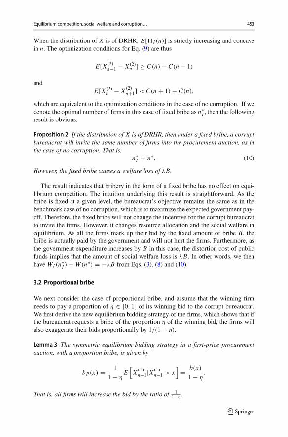
Equilibrium competition, social welfare and corruption… 453
When the distribution of X is of DRHR, E[�I (n)] is strictly increasing and concavein n. The optimization conditions for Eq. (9) are thus
E[X (2)n−1 − X (2)
n ] ≥ C(n) − C(n − 1)
andE[X (2)
n − X (2)n+1] < C(n + 1) − C(n),
which are equivalent to the optimization conditions in the case of no corruption. If wedenote the optimal number of firms in this case of fixed bribe as n∗
I , then the followingresult is obvious.
Proposition 2 If the distribution of X is of DRHR, then under a fixed bribe, a corruptbureaucrat will invite the same number of firms into the procurement auction, as inthe case of no corruption. That is,
n∗I = n∗. (10)
However, the fixed bribe causes a welfare loss of λB.
The result indicates that bribery in the form of a fixed bribe has no effect on equi-librium competition. The intuition underlying this result is straightforward. As thebribe is fixed at a given level, the bureaucrat’s objective remains the same as in thebenchmark case of no corruption, which is to maximize the expected government pay-off. Therefore, the fixed bribe will not change the incentive for the corrupt bureaucratto invite the firms. However, it changes resource allocation and the social welfare inequilibrium. As all the firms mark up their bid by the fixed amount of bribe B, thebribe is actually paid by the government and will not hurt the firms. Furthermore, asthe government expenditure increases by B in this case, the distortion cost of publicfunds implies that the amount of social welfare loss is λB. In other words, we thenhave WI (n∗
I ) − W (n∗) = −λB from Eqs. (3), (8) and (10).
3.2 Proportional bribe
We next consider the case of proportional bribe, and assume that the winning firmneeds to pay a proportion of η ∈ [0, 1] of its winning bid to the corrupt bureaucrat.We first derive the new equilibrium bidding strategy of the firms, which shows that ifthe bureaucrat requests a bribe of the proportion η of the winning bid, the firms willalso exaggerate their bids proportionally by 1/(1 − η).
Lemma 3 The symmetric equilibrium bidding strategy in a first-price procurementauction, with a proportion bribe, is given by
bP (x) = 1
1 − ηE
[X (1)n−1|X (1)
n−1 > x]
= b(x)
1 − η.
That is, all firms will increase the bid by the ratio of 11−η
.
123

454 M. Xu, D. Z. Li
Under the proportional bribe, the rent for the winning firm is
RP (n) = (1 − η)bP (X (1)n ) − X (1)
n = b(X (1)n ) − X (1)
n ,
where the subscript ‘P’ denotes the case of proportional bribe. It is obvious that thegovernment’s payoff function is no longer the same as in Eq. (2), and it is now
�P (n) = V − bP (X (1)n ) − C(n) = V − b(X (1)
n )
1 − η− C(n).
The corrupt bureaucrat receives the bribe B(n) = ηbP (X (1)n ). As before, the total
social welfare is the sum of the payoffs of the three parties, minus the distortion costof public funds, which is
WP (n) = V − X (1)n − λ
1 − ηb(X (1)
n ) − (1 + λ)C(n).
The corrupt bureaucrat’s payoff function is a weighted average of his bribe and thegovernment’s payoff, and his problem is thus
max E[UP (n)] = αE[�P (n)] + (1 − α)ηE[bP (X (1)n )]. (11)
Under the DRHR assumption, we know that E[�P (n)] is concave, and ηE[bP (X (1)n )]
is convex in n, and this does not imply that a convex combination of them is necessarilyconcave. However, E[UP (n)] can be rewritten as
E[UP (n)] = α(V − C(n)) − α − (1 − α)η
1 − ηE[X (2)
n ].
We know E[X (2)n ] is strictly decreasing and convex in n, and thus E[UP (n)] is strictly
concave if α − (1 − α)η > 0.
Lemma 4 If the distribution of X is of DRH R and η < α1−α
, then E[UP (n)] is strictlyconcave in n.
The condition of η < α1−α
means that the bribe proportion is small relative to theweight of government payoff in the corrupt bureaucrat’s utility function. Consideringthat the sizes of public procurements usually are quite large, we could reasonably thinkthat η is normally small and this condition would be satisfied in most cases. If it doesnot hold and η ≥ α
1−α, we would be in the environments of extreme corruption, in
which either the weight α is quite small or the bribe proportion η is quite large, thenthe bureaucrat’s objective function, E[UP (n)], is strictly decreasing in n, and thus,the optimal number of firms is equal to 1, i.e., the single bid scenario. The problemthen becomes trivial in this case. Here, we consider the non-trivial scenario underthe condition of η < α
1−α. Denote n∗
P as the optimal number of firms in the case ofproportional bribe, and then we have the following result.
123
Equilibrium competition, social welfare and corruption… 455
Proposition 3 If the distribution of X is of DRHR and 0 < η < α1−α
, then under aproportional bribe, a corrupt bureaucrat invites either fewer or more firms into theprocurement auction than in the benchmark case of no corruption. Specifically,
(i) if α ∈ [0, 1/2], then n∗P ≤ n∗;
(ii) if α ∈ [1/2, 1], then n∗P ≥ n∗.
The optimal number of firms under a proportional bribe can be either greater orsmaller than the competition without corruption, which depends on the relative mag-nitude of two opposite effects: (i) the first term of Eq. (11), E[�P (n)], implies thathe may encourage competition, as firms raise their bids and therefore the distributionof bids turns out to be more dispersed than before, which decreases the level of com-petition in the auction; (ii) the second term of Eq. (11) implies that the bureaucratmay discourage competition, as E[bP (X (1)
n )] is decreasing in n. Thus, the effect of theproportional bribe on the competition depends on how much the bureaucrat weightshis individual interest relative to the government payoff. As a result, when the corruptbureaucrat cares more about his personal interest, α < 1/2, he will dampen competi-tion in the auction, and when he cares more about the government payoff, α > 1/2,he will encourage competition.
Finally, let us turn to the socially efficient number of firms in different cases. Ifwe denote the socially optimal number of firms in the cases of fixed and proportionalbribe by n∗∗
I and n∗∗P respectively, then we have the following result.
Proposition 4 The order of socially efficient numbers of firms is
n∗∗ = n∗∗I < n∗∗
P .
This result suggests that the effects of bribery on efficient competition vary on theformats of bribery. Although the fixed bribe does not change the socially efficientcompetition, the bribery incurs some social cost. Specifically, we have
WI (n∗∗I ) + λB = W (n∗∗),
from Eqs. (3) and (8). Under proportional bribery, firms exaggerate their bids andthe distribution of the winning bids becomes more dispersed, which implies a largernumber of firms for social efficiency.
Let us extend the previous numerical example to the case of corruption, which helpsus to understand the various effects of corruption.
Example 2 We introduce corruption into our previous Example 1 of uniform distribu-tion. We have already known that E[X (1)
n ] = Vn+1 and E[X (2)
n ] = 2Vn+1 . In the case of
a fixed bribe B, we have
E[UI (n)] = αE[�I (n)] + (1 − α)B.
The optimal number of firms is n∗I = n∗ as shown in Proposition 2.
123
456 M. Xu, D. Z. Li
In the case of proportional bribe, we have
E[UP (n)] = α(V − C(n)) − α − (1 − α)η
1 − ηE[X (2)
n ] =[α − α − (1 − α)η
1 − η
2
n + 1
]
×V − αnc.
If η ≥ α1−α
, then E[UP (n)] is strictly decreasing in n, so n∗P = 1, that is the minimum
possible number of firms. The problem then becomes trivial in this case.Let us consider 0 < η < α
1−α, then E[UP (n)] is concave inn. The optimal condition
for n∗P is
n(n + 1) ≤ α − (1 − α)η
(1 − η)α· 2V
c< (n + 1)(n + 2).
– If α ≤ 1/2, we have α−(1−α)η(1−η)α
≤ 1, and then n∗P ≤ n∗. For example, if c = 2
and V = 36, we have already known n∗ = 5. Let us now select α = 1/3 andη = 1/4 such that α−(1−α)η
(1−η)α= 2/3, we have the optimal number of firms under
the proportional bribe, n∗P = 4, which is less than n∗ = 5.
– If α ≥ 1/2, we have α−(1−α)η(1−η)α
≥ 1, and then n∗P ≥ n∗. For example, if c = 2
and V = 36, and then n∗ = 5. Now we select α = 2/3 and η = 2/5 such thatα−(1−α)η
(1−η)α= 4/3, we have the optimal number of firms under the proportional
bribe, n∗P = 6, which is greater than 5.
4 Further discussion
4.1 Second-price procurement auctions
It is a natural question whether corruption has different effects on competition in thesecond-price procurement auction. As we know, bidding the true production cost Xi isa weakly dominant strategy in the second-price auction. In the benchmark case of nocorruption, it is easy to show that the result of Proposition 1 holds in the second-pricescenario. We now consider the results with corruption.
In the case of fixed bribe, the bureaucrat requests the winning firm to pay a fixedbribe of B after the auction, and then the fixed bribe amount appears to be a part offirms’ cost condinional on winning the auction. As the virtual cost for firm i is nowX ′i = Xi + B, bidding X ′
i is thus a weakly dominant strategy for firm i , and all firmswill mark up their bids by the fixed amount of B. Therefore, the fixed bribe has thesame effect on the bidding function from Lemma 2, and we can derive the same resultof Proposition 2 in the second-price setting.
Considering the case of a proportional bribe, we assume that the winning firm needsto pay a proportion of η of its revenue to the corrupt bureaucrat. We have the followingresult:
Lemma 5 If the winning firm needs to pay a proportion of η of its revenue to thecorrupt bureaucrat in the second-price procurement auction, bidding 1
1−ηtimes the
production cost is a weakly dominant strategy.
123

Equilibrium competition, social welfare and corruption… 457
Recalling Lemma 3, it is obvious that the results of a proportional bribe all remainthe same in the second-price auction setting. In sum, the Revenue Equivalence resultbetween the first- and second-price auctions still holds with corruption. Therefore, theeffects of corruption on equilibrium competition and social welfare are the same inboth first- and second-price procurement auctions.
4.2 Information disclosure
As shown in the recent literature (Johnson andMyatt 2006; Ganuza and Penalva 2010;Jewitt and Li 2015), information disclosure may induce more dispersed distributionof consumers’ valuations. The intuition is that when consumers’ preferences are hor-izontally differentiated, revealing product information may drive up the valuations ofsome consumers, while driving down those of others; therefore, the distribution ofposterior consumer valuations becomes more dispersed.
A similar argument can be applied in our context of public procurements. Forexample, the firmsmayhave different expertise or areas of specialization, and revealinginformation on the details of the public contract may have differentiated impactson their cost estimates. That information may be good news for some firms whenthey find it is a good match for their areas of specialization, whereas it may be badnews for others. Consequently, the distribution of firms’ cost estimates becomes moredispersed under information disclosure. Though similar arguments and results havebeen provided inGanuza and Penalva (2010, Theorem6) and Szech (2011, Proposition2), we think it would still be desirable to provide some further discussions here,where we explicitly consider the distortion cost of public funds and the possibility ofcorruption in public procurement auctions.
Let us denote Y as the new cost for the firms after information disclosure, and thecorrespondingdistribution isG(·). Comparedwith the initial cost of X withdistributionF(·), we know the distribution of Y is more dispersed, or formally, X �disp Y , definedas follows:
Definition 2 The random variable X is smaller than Y in the dispersive order, denotedby X �disp Y , if
F−1(q) − F−1(p) ≤ G−1(q) − G−1(p)
for all 0 < p < q < 1.
It is intuitive that when the distribution of firms’ cost estimates becomes moredispersed, the procurement auction becomes less competitive than before, and thewinning rent of the firms will increase. It is then natural that, in general, more firmsneed to be invited in this case. The similar results hold in our procurement settings withor without corruption. Specifically, let n∗ (n∗∗) denote the optimal (socially efficient)number of firms under the distribution F(·); let n̂∗ (n̂∗∗) denote the optimal (sociallyefficient) number of firms under the distribution G(·); and the subscripts ‘I ’ and‘P’ denote the cases of fixed bribe and proportional bribe, respectively. Proposition 5below then shows that, for government payoff and socialwelfaremaximization,with orwithout corruption, andwith a fixed bribe or a proportional bribe, when the distribution
123
458 M. Xu, D. Z. Li
of firms’ costs become more dispersed under information disclosure, more firms needto be invited for the competition in the public procurement.
Proposition 5 If X �disp Y , and the distribution of F(·) and G(·) are DRHR, thenwe have
n∗ ≤ n̂∗, n∗∗ ≤ n̂∗∗;n∗I ≤ n̂∗
I , n∗∗I ≤ n̂∗∗
I ;n∗P ≤ n̂∗
P , n∗∗P ≤ n̂∗∗
P .
The resultsmay raise the concern that, with the possibility of informationmanipula-tion, the bureaucrat canmake it impossible to infer the existence of corruption from theobservation of the number of firms invited into the procurement auction. For example,suppose that the ex ante cost distribution is F(·), the optimal number of firms withoutcorruption is n∗, and that number under a proportional bribe is n∗
P which is smallerthan n∗. If the bureaucrat has the discretion of manipulating information, then he caninduce a more dispersed cost distribution of G(·) through information disclosure, andinvite n̂∗
P firms into the auction, which is larger than n∗P and possibly closer to n∗.
If the government is not aware of the change of underlying cost distribution, it maybelieve that the bureaucrat is honest as he chooses a number of firms that is close ton∗.
4.3 Government regulations
The above results show that the effects of corruption on equilibrium competition andsocial welfare vary across different forms of bribery. They also raise the questionof optimal and effective regulations by a central government to ensure sound publicservices and improve socialwelfare. In the case of fixed bribe, although itwill not affectthe equilibrium competition, it does incur more public spending by the government,which induces social welfare loss. To prevent corruption in that form, the governmentneeds to conduct a strict audit of the project budget, guarantee sufficient transparencyover the entire competition process, and carefully evaluate the cost estimates reportedby firms.
In the case of proportional bribe, the corrupt bureaucratmay favor either less ormorecompetition in the auction, depending on how much he weights his private interestrelative to the government payoff. In the case of extreme corruption, e.g., η ≥ α
1−α,
the bureaucrat prefers as less competition as possible and will invite only a singlefirm to the auction. In the case of moderate corruption, e.g., η < α
1−α, if the corrupt
bureaucrat weights his private interest much higher (i.e., α < 1/2 in Proposition 3),he would also have incentives to dampen competition in the auction. In this case,it would be helpful for the government or regulators to impose requirements on theminimum number of firms in public procurements. For example, in the regulationsfor public procurements in the European Union, a public authority must invite at least
123

Equilibrium competition, social welfare and corruption… 459
five candidates possessing the capabilities required to submit tenders in the restrictedprocedure.10
5 Concluding remarks
It is important to study the mutual interaction between corruption and competition inpublic procurements. In this paper, we examine the specific effects of corruption onequilibrium competition and social welfare in a public procurement auction. In ourmodel, it is costly for a government to invite the firms to the auction, and a bureaucratwho runs the auction on behalf of the governmentmay request a bribe from thewinningfirm. The bribery can be in the form of either a fixed bribe or a proportional bribe.
We show that the effects of corruption on equilibriumcompetition and socialwelfarevary across different forms of bribery. First, under a fixed bribe, corruption does notaffect equilibrium competition, but it does induce social welfare loss in equilibrium.This is because, in expectation of the fixed bribe, all firms will mark-up their bids bythe same amount of bribe, which will not change the bureaucrat’s incentive to invitefirms, and the level of equilibrium competition remains the same as before. In this case,it is the government that pays the fixed bribe in the end, and the increased governmentspending implies social welfare loss due to the distortion cost of public funds.
Second, under a proportion bribe, we show that all firms increase their equilibriumbids proportionally, and corruption may induce either less or more competition inequilibrium, depending on how the bureaucrat weights his private interest relative tothe government payoff. The intuition is straightforward. On the one hand, as firms’equilibrium bids become more dispersed, the auction becomes less competitive thanbefore, which negatively affects the government’s payoff. On the other hand, lesscompetition is beneficial for the bureaucrat’s private interest, as it impliesmore briberyfrom the winning firm. As a result, the relative magnitude between these two oppositeeffects determines the level of equilibrium competition. For instance, if the bureaucratcares more about his private interest, he will invite fewer firms; otherwise, he willinvite more firms.
We further discuss some policy implications of our model. First, our results suggestthat the optimal regulation rules are necessarily contingent on the specific forms ofcorruptions. Therefore, it is essential to investigate the exact and dominant formsof bribery before proposing relevant regulation rules (Sect. 4.3). Second, given thatinformation disclosure may dampen equilibrium competition in public procurements,a corrupt bureaucrat may intentionally manipulate information for his benefits. It isthen crucial for regulators to carefully design the rules of information disclosure inpublic procurements (Sect. 4.2). Third, we also show that themain results of ourmodelstill hold in other auction formats (Sect. 4.1).
There are many possible directions for further extending the framework developedin this paper. For example, we may consider a model where a corrupt bureaucrat mayhave more discretion in manipulating the auction rules, besides just controlling the
10 See http://europa.eu/youreurope/business/public-tenders/rules-procedures/index_en.htm. Updated inSep. 2018.
123

460 M. Xu, D. Z. Li
number of invited firms. Another interesting example would be scoring auctions withcostly participation, which are common in public procurements. In a scoring auction,the quality information is commonly non-verifiable, and therefore a corrupt bureaucratmay also manipulate the scoring rules in exchange for a bribe.
Acknowledgements We are grateful to the editor in charge and two referees, whose comments and sugges-tions greatly improved this paper. We thank Ian Jewitt, Sanxi Li, Jaimie Lien, Thomas Renstrom, BibhasSaha, Xi Weng, Lixin Ye and Jie Zheng for helpful comments and discussions. We also thank the attendantsof the seminars at the Chinese University of Hong Kong, Durham University and Renmin University ofChina, as well as the conference participants of GAMES 2016, CMES 2016 and AMES 2016 for theirhelpful comments and suggestions.
Open Access This article is distributed under the terms of the Creative Commons Attribution 4.0 Interna-tional License (http://creativecommons.org/licenses/by/4.0/), which permits unrestricted use, distribution,and reproduction in any medium, provided you give appropriate credit to the original author(s) and thesource, provide a link to the Creative Commons license, and indicate if changes were made.
Appendix: Omitted Proofs
Proof of Lemma 1 For result (i), it holds that E[X (1)n ] = ∫ V
0 xdF (1)n (x) = ∫ V
0(1 − F (x))n dx , which implies
E[X (1)n+1 − X (1)
n ] = −∫ V
0F (x) (1 − F (x))n dx < 0.
As f (x) > 0, then E[X (1)n+1 − X (1)
n ] is strictly increasing in n. We then show that
E[X (1)n ] is strictly increasing and strictly convex in n. Furthermore, as f (x) > 0, it
is clear that limn→∞ E[X (1)n ] = limn→∞
[∫ V0 (1 − F (x))n dx
]= 0.
For result (ii), we first have
F (1)n (x) = 1 − F̄(x)n and F (2)
n (x) = 1 − F̄(x)n−1[1 + (n − 1)F(x)], (12)
where F̄(x) = 1 − F(x) is the survival function. It then follows that
E[X (2)n − X (2)
n+1] =∫ V
0[F (2)
n+1(x) − F (2)n (x)]dx =
∫ V
0
F2(x)
f (x)dF (1)
n (x) > 0.
When F(·) is of DRHR, the function h(x) = F2(x)f (x) is increasing. Thus, E[X (2)
n ]is strictly decreasing and convex in n. Furthermore, as limx→0 h(x) = 0, we havelimn→∞ E[X (2)
n − X (2)n+1] = 0.
For result (iii), we have E[X (2)n − X (1)
n ] = ∫ V0 [F (1)
n (x) − F (2)n (x)]dx =∫ V
0F(x)f (x)dF
(1)n (x). Let h(x) = F(x)
f (x) , it is increasing under the DRHR assumption,
and limx→0 h(x) = 0. Following the same proof as in (i), we obtain the results. �
123
Equilibrium competition, social welfare and corruption… 461
Proof of Proposition 1 If F(·) is DRHR, E[R(n)] = E[X (2)n −X (1)
n ] is strictly decreas-ing in n, then
E[X (2)n − X (1)
n
]> E
[X (2)n+1 − X (1)
n+1
]⇔ E
[X (2)n − X (2)
n+1
]> E
[X (1)n − X (1)
n+1
].
From n∗ = argmax E[�(n)], the optimization condition implies
E[�(n∗) − �(n∗ − 1)
] ≥ 0 > E[�(n∗ + 1) − �(n∗)],
which is equivalent to
E[X (2)n∗−1 − X (2)
n∗]
≥ C(n∗) − C(n∗ − 1)
andE
[X (2)n∗ − X (2)
n∗+1
]< C(n∗ + 1) − C(n∗).
Similarly, for n∗∗ = argmax E[W (n)], we have1
1 + λE[X (1)
n∗∗−1 − X (1)n∗∗ ] + λ
1 + λE[X (2)
n∗∗−1 − X (2)n∗∗ ] ≥ C(n∗∗) − C(n∗∗ − 1)
and
1
1 + λE
[X (1)n∗∗ − X (1)
n∗∗+1
]+ λ
1 + λE
[X (2)n∗∗ − X (2)
n∗∗+1
]< C(n∗∗ + 1) − C(n∗∗).
As for all n,
E[X (2)n−1 − X (2)
n
]>
1
1 + λE
[X (1)n−1 − X (1)
n
]+ λ
1 + λE
[X (2)n−1 − X (2)
n
];
thus, the result of n∗ ≥ n∗∗ is obvious. �Proof of Lemma 2 Denote the new increasing bidding strategy in a symmetric equi-librium by bI (x), and bidders i = 2, . . . , n stick to this strategy. Denote Y =min {X2, . . . , Xn} = X (1)
n−1, and then bI (Y ) is the lowest bid of those bidders. Bidder1 wins the auction whenever his bid β < bI (Y ) bidder, and he chooses the bid tomaximize his expected payoff
E[(β − x) · 1β<bI (Y )
] = (β − x − B)[1 − F (1)
n−1
(b−1I (β)
)].
Taking the first-order condition with respect to β, it follows that
[1 − F (1)
n−1
(b−1I (β)
)]− (β − x − B)
f (1)n−1
(b−1I (β)
)
b′I
(b−1I (β)
) = 0.
123
462 M. Xu, D. Z. Li
In symmetric equilibrium, β = bI (x), and thus
b′I (x)
[1 − F (1)
n−1 (x)]
− b (x) f (1)n−1 (x) = − (x + B) f (1)
n−1 (x) ,
or equivalently,
d
dx
[bI (x)
[1 − F (1)
n−1 (x)]]
= − (x + B) f (1)n−1 (x) .
Since b (V ) = V + B, then
bI (x) =∫ V
x(y + B) d
F (1)n−1 (y)
F̄ (1)n−1 (x)
= (x + B) +∫ V
x
F̄ (1)n−1 (y)
F̄ (1)n−1 (x)
dy.
�Proof of Lemma 3 Denote the new increasing bidding strategy in a symmetric equi-librium by bP (x), and bidders i = 2, . . . , n stick to this strategy. Denote Y =min {X2, . . . , Xn} = X (1)
n−1, and then bP (Y ) is the lowest bid of those bidders. Bid-der 1 wins the auction whenever his bid β < bP (Y ) bidder, and he chooses bid tomaximize his expected payoff
E[((1 − η) β − x) · 1β<bP (Y )
] = [(1 − η) β − x][1 − F (1)
n−1
(b−1P (β)
)].
Taking the first-order condition with respect to β, it follows that
(1 − η)[1 − F (1)
n−1
(b−1P (β)
)]− [(1 − η) β − x]
f (1)n−1
(b−1P (β)
)
b′P
(b−1P (β)
) = 0.
In symmetric equilibrium, β = bP (x), and thus
b′P (x)
[1 − F (1)
n−1 (x)]
− bP (x) f (1)n−1 (x) = − x f (1)
n−1 (x)
1 − η,
or equivalently,
d
dx
[bP (x)
[1 − F (1)
n−1 (x)]]
= − x f (1)n−1 (x)
1 − η.
Since b (V ) = V / (1 − η), then
bP (x) =∫ V
x
y
1 − ηdF (1)n−1 (y)
F̄ (1)n−1 (x)
= 1
1 − ηb (x) .
123
Equilibrium competition, social welfare and corruption… 463
�Proof of Proposition 3 If 0 < η < α
1−α, Lemma 4 implies E[UP (n)] is strictly concave
in n. Then, the optimization conditions for n∗P are
α − (1 − α)η
1 − ηE
[X (2)n−1 − X (2)
n
]≥ α(C(n) − C(n − 1))
andα − (1 − α)η
1 − ηE
[X (2)n − X (2)
n+1
]< α(C(n + 1) − C(n)).
Compared with the optimization conditions for n∗, we imply that,If α−(1−α)η
1−η≤ α, i.e., α ≤ 1/2, then we have n∗
P ≤ n∗.If α−(1−α)η
1−η> α, i.e., α > 1/2, we have n∗
P > n∗. �Proof of Proposition 4 Apparently, n∗∗
I = n∗∗, in which both follow the same opti-mization conditions
φ(n) ≥ C(n) − C(n − 1)
andφ(n + 1) < C(n + 1) − C(n),
whereφ(n) = 11+λ
E[X (1)n−1 − X (1)
n
]+ λ
1+λE[X (2)
n−1−X (2)n ]. Under proportional bribe,
the optimization conditions are
φ(n) + αη
(1 + α)(1 − η)E
[X (2)n−1 − X (2)
n
]≥ C(n) − C(n − 1)
andφ(n + 1) + αη
(1 + α)(1 − η)E
[X (2)n − X (2)
n+1
]< C(n + 1) − C(n).
Thus, we have n∗∗P > n∗∗. �
Proof of Lemma 5 Let us denote the increasing bidding function by bP (x) for a firmwith cost x . Given other firms that follow this strategy, we derive the equilibrium forfirm 1. Denote Y = min{X2, . . . , Xn}, and then bP (Y ) is the lowest bid of those n−1rival bidders. Bidder 1 wins the auction whenever his bid β < bP (Y ). The objectivefunction is
E[((1 − η)bP (Y ) − x) · 1β<bP (Y )
] = E
[(bP (Y ) − x
1 − η
)· 1β<bP (Y )
].
It is clear that β = x1−η
is a weakly dominant strategy. �Proof of Proposition 5 From Theorem 5.3.1 of Arnold et al. (2008), we have the fol-lowing recurrence relationship
i E[X (i+1)n
]+ (n − i)E
[X (i)n
]= nE
[X (i)n−1
].
123

464 M. Xu, D. Z. Li
Therefore,
E[X (2)n−1 − X (2)
n
]= 2
nE
[X (3)n − X (2)
n
]≤ 2
nE
[Y (3)n − Y (2)
n
]= E
[Y (2)n−1 − Y (2)
n
],
where the inequality is implied by the result that E[X ( j)n −X ( j−1)
n ] ≤ E[Y ( j)n −Y ( j−1)
n ].Thus, we can conclude that n∗ ≤ n̂∗. Similarly, we can also prove the result thatn∗∗ ≤ n̂∗∗. From Proposition 2, it is clear that n∗
I = n∗ and n̂∗I = n̂∗, and then
n∗I ≤ n̂∗
I . From Proposition 4, we have n∗∗I ≤ n̂∗∗
I .Now let us prove that n∗
P ≤ n̂∗P . First, if n
∗P is the corner solution that n∗
P = 1, thenn∗∗P ≤ n̂∗∗
P is clearly true as n̂∗∗P ≥ 1. Second, if n∗
P is an interior solution such thatthe optimization conditions for n∗
P are
α − (1 − α)η
1 − ηE
[X (2)n−1 − X (2)
n
]≥ α(C(n) − C(n − 1))
andα − (1 − α)η
1 − ηE
[X (2)n − X (2)
n+1
]< α(C(n + 1) − C(n)).
Thus, we can conclude that n∗P ≤ n̂∗
P . The similar result n∗∗P ≤ n̂∗∗
P can be impliedfrom the optimization conditions as in the Proof of Proposition 4. �
References
AcemogluD,Verdier T (2000)The choice betweenmarket failures and corruption.AmEconRev 90(1):194–211
Ades A, Di Tella R (1999) Rents, competition, and corruption. Am Econ Rev 89(4):982–993Alexeev M, Song Y (2013) Corruption and product market competition: an empirical investigation. J Dev
Econ 103:154–166Amir R, Burr C (2015) Corruption and socially optimal entry. J Pub Econ 123:30–41Arnold BC, Balakrishnan N, Nagaraja HN (2008) A first course in order statistics. SIAM, PhiladelphiaArozamena L,Weinschelbaum F (2009) The effect of corruption on bidding behavior in first-price auctions.
Eur Econ Rev 53:645–657Auriol E (2006) Corruption in procurement and public purchase. Int J Indus Organ 24:867–885Basu K (2011) Why, for a class of bribes, the act of giving a bribe should be treated as legal. Ministry of
Finance, Government of India, Working PaperBliss C, Di Tella R (1997) Does competition kill corruption? J Polit Econ 105(5):1001–1023Burguet R (2017) Procurement design with corruption. Am Econ J Microecon 9(2):315–341Burguet R, Che Y (2004) Competitive procurement with corruption. RAND J Econ 35(1):50–68Burguet R, Perry MK (2009) Preferred suppliers in auction markets. RAND J Econ 40(2):283–295Celentani M, Ganuza JJ (1999) Corruption and the Hadleyburg effect. Working Paper No. 382, Department
of Economics, Universitat Pompeu FabraCelentani M, Ganuza JJ (2002) Corruption and competition in procurement. Eur Econ Rev 46:1273–1303Compte O, Jehiel P (2002) On the value of competition in procurement auctions. Econometrica 70(1):343–
355Compte O, Lambert-Mogiliansky A, Verdier T (2005) Corruption and competition in procurement auctions.
RAND J Econ 36(1):1–15Emerson P (2006) Corruption, competition and democracy. J Dev Econ 81:193–212Ganuza JJ, Penalva JS (2010) Signal orderings based on dispersion and the supply of private information
in auctions. Econometrica 78(3):1007–1030
123
Equilibrium competition, social welfare and corruption… 465
Jain AK (2001) Corruption: a review. J Econ Sur 15(1):71–121Jewitt I, Li D (2015) Cheap-talk information disclosure in auctions. Working PaperJohnson J, Myatt D (2006) On the simple economics of advertising, marketing, and product design. Am
Econ Rev 96(3):756–784Inderst R, OttavianiM (2012) Competition through commissions and kickbacks. AmEconRev 102(2):780–
809Krishna V (2002) Auction theory. Academic, New YorkLaffont JJ, Tirole J (1987) Auctioning incentive contracts. J Polit Econ 95(5):921–937Lee J, Li D (2018) Sequential search auctions with a deadline. SSRN Working Paper No. 3133797Lengwiler Y, Wolfstetter E (2006) Corruption in procurement auctions. In: Dimitri N, Piga G, Spagnolo G
(eds) Handbook of procurement. Cambridge University Press, Cambridge, pp 412–429Levin D, Smith J (1994) Equilibrium in auctions with entry. Am Econ Rev 84(3):585–599Li D (2017) Ranking equilibrium competition in auctions with participation costs. Econ Lett 153:47–50McAfee P, McMillan J (1987) Auctions with entry. Econ Lett 23:343–347Menezes FM, Monteiro PK (2006) Corruption and auctions. J Math Econ 42:97–108Myerson R (1981) Optimal auction design. Math Oper Res 6(1):58–73Rose-Ackerman S (1978) Corruption: a study of political economy. Academic, New YorkShleifer A, Vishny R (1993) Corruption. Q J Econ 108(3):599–617Szech N (2011) Optimal advertising of auctions. J Econ Theory 146:2596–2607
Publisher’s Note Springer Nature remains neutral with regard to jurisdictional claims in published mapsand institutional affiliations.
123