T.P. 3493

EQUILIBRIUM CONSTANTS FOR A GAS-CONDENSATE

SYSTEM

A. E. HOFFMANN, J. S. CRUMP AND C. R. HOCOTT, MEMBER AIME, HUMBLE OIL AND REFINING CO., HOUSTON, TEX.

ABSTRACT

Planning of the efficient operation of a gas-condensate re;;er­voir requires a knowledge not only of the gross phase behavior of the system but also of the equilibrium distribution of the various components between the ga5 and condensate phases. This equilibrium distribution can be calculated with appro­priate equilibrium constants. In this paper are presente::l equilibrium constants determined experimentally for the oil and gas phases initially present in the same reservoir and for the gas and condensate phases of the gas cap material at a series of pressures below the original reservoir pressure. Also presented is a method for the correlation of the experimentalb determined equilibrium constants. The utility of the correla­tion is demonstrated further by an example of its use in adjusting the equilibrium data to permit their application to another gas-condensate system of similar composition.

INTRODUCTION

Planning of the efficient operation of a gas-condensate reser­voir requires a thorouugh knowledge not only of the gros' phase behavior of the particular hydrocarbon system but also of the equilibrium distribution of the various components between the gas and condensate phases. At the initial condi­tions of reservoir temperature and pressure, the original hydrocarbon materials in a gas-condensate reservoir or in the gas-cap of an associated reservoir exist in a single, homogene­ous vapor phase. However, some condensation of hydrocarbons to a liquid phase usually occurs in the reservoir as pressure declines incident to production. Because of this condensation, the produced gas changes composition continuously. The com­position of the produced gas, as well as that of the condensed

1References given at end of paper. Manuscript received in the office of the Petroleum Branch, July 29, 1952.

Paper presented at the Fall Meeting of the Petroleum Branch in Hous­ton, Oct. 1-3, 1952.

liquid, can be calculated from the composition of the original reservoir material through the application of appropriate equi­librium comtants or "K"-values provided these values are known.

Equilibrium constants have been used for many years in problems of surface separation of gas and oil and natural gasoline recovery. However, no satisfactory equilibrium data at reservoir conditions have been available for the higher boil­ing hydrocarbons which acquire abnormal volatility at high pressure and are therefore present in the gas phase in con­densate reservoirs. Early work in this field indicated that the behavior of the higher boiling hydrocarbons largely decermines the behavior of gas-condensate systems at high pre3sure.1

Con'equently, a portable test unit was designed to permit determination of the distribution of the heavier hydrocarbom between the gas and liquid phases of a gas-condensate system. This paper describes the test equipment and presents the results of an investigation of the reservoir fluids from an asso­ciated oil and gas reservoir in the Frio formation in Southwest Texas. Also presented is a method for correlation of the experi­mentally determined equilibrium constants, together with an example of the use of the method in adjusting these data for application to another gas-condensate system of similar composition.

FIELD TESTING AND SAMPLING

In order to determine the compositions of the re'3ervoir fluids, field samples were secured from two different wells, one completed in the oil zone, and one completed in the gas cap.

The oil well was completed through perforations in 51/z-in. casing at a depth of 6,822-6,828 ft subsea. Pressure and tem­perature traverses made in the well indicated the pressure and temperature to be 3,831 psig and 201 °F, respectively, at a depth of 6,828 ft subsea. Subsurface samples were taken from this well after a four-hour shut-in period.

Vol. 198, 1953 SPE 219-G PETROLEUM TRANSACTIONS, AIME l

T.P. 3493 EQUILIBRIUM CONSTANTS FOR A GAS-CONDENSATE SYSTEM

FIG. 1 - PORTABLE APPARATUS FOR GAS-CONDENSATE TESTING.

The gas well was completed through perforations in 7-in. casing at a depth of 6,760-6,788 ft subsea. For testing, the well was placed on production and the rates of gas and condensate production were determined at frequent intervals with care­fully calihrated equipment. After the rates of production. had become constant, samples of gas and liquid were taken from the separator. In addition to the conventional gas samples, separate portions of the gas were passed through charcoal tubes for adsorption and subsequent analysis of the butanes and heavier hydrocarbon content of the gas.

At the time of sampling, the well was producing at a rate of 5,718 Mcf of gas and 162.8 bbl of separator liquid per day. The tubing pressure was 3,100 psig, and the separator pressure and temperature were 785 psig and 83°F, respectively.

At the conclusion of the sampling the well was shut in, and about 36 hours later pressure and temperature traverses were made in the well. The pressure and temperature were indi­cated to be 3,822 psig and 201 °F, respectively, at a depth of 6, 788 ft subsea.

For further testing of the gas well a specially designed portable test unit was used for the determination of the phase behavior and for the sampling incident to the determination of equilibrium constants at reservoir temperature at various pressures for the gas-cap material.

PORTABLE TEST EQUIPMENT

The portable equipment used in the investigation was de­signed for operation at pressures up to wellhead pressure and was constructed for 10,000 psi maximum working pressure. Oil baths are used for temperature control. They are heated with immersion heaters powered by a portable, gasoline engine driven, 2,500 watt, llO volt, 60 cycle AC generator, which also provides power for stirrers, lights, and relays. All electrical equipment is provided with ample safty devices to minimize spark hazard. Insofar as possible, 18-8 stainless steel was used throughout the pressure system to reduce corrosion and for safety during low temperature operation. The equipment is as!':embled on an aluminum panel and framework equipped with rollers and mounted on a half-ton pickup truck. Photo­graphs of the unit are shown in Fig. 1.

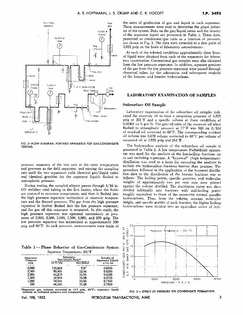
The test equipment consists essentially of two gas-liquid separators, together with auxiliary equipment for measuring the rates of gas flow and of liquid accumulation and for the sampling of each phase. A flow diagram of the equipment is shown in Fig. 2. The first separator, referred to as the high pressure separator, is operated at reservoir temperature at a series of pressures. The second separator, referred to as the low pressure separator, is usually operated at pressures and temperatures in the range of those of the field separator. The usual test procedure involves the operation of these separators in series, with the gas from the first separator flashed into the second separator. The heavy hydrocarbon fractions in the gas phase from the high pressure separator are condensed to the liquid phase in the low pressure separator. By this procedure, these heavy hydrocarbon fractions may be concentrated suffi­ciently to permit the rncuring of an adequate sample for an analysis of these fractions. From a composite of this liquid analysis with that of the gas leaving the low pressure separator, an extended analysis can be obtained of the gas leaving the high pressure separator. Such a complete analysis is not possible with conventional gas samples or charcoal samples.

TESTING AND SAMPLING GAS-CAP MATERIAL

The method used in obtaining a continuous representative sample of the well stream is essentially that described by Flaitz and Parks.2 By this method an aliquot of the well stream is obtained through a special line sampler inserted in the flow line near the well head. For accurate testing it is essential that the well be producing at a rate sufficient to pre­vent accumulation of liquid in the tubing and to insure homogeneous flow. The proper sampling rate is determined by by-passing the high pressure separator, operating the low

2 PETROLEUM TRANSACTIONS, AIME Vol. 198, 1953

A. E. HOFFMANN, J. S. CRUMP AND C. R. HOCOTT T.P. 3493

::-rem Field

Separator

10,000 #

Heise

10,000 #

Crosby

From Well

' ' ' ' ' I

L _J Heater

Ind

FIG. 2-FLOW DIAGRAM, PORTABLE APPARATUS FOR GAS-CONDENSATE TESTING.

pressure separator of the test unit at the same temperature and pressure as the field separator, and varying the sampling rate until the two separators yield identical gas/liquid ratios and identical gravities for the separator liquids flashed to atmospheric pressure.

During testing, the sampled aliquot passes through 3/16 in. OD stainless steel tubing to the first heater, where the fluids are restored to reservoir temperature, and then is flashed into the high pressure separator maintained at reservoir tempera­ture and the desired pressure. The gas from the high pressure separator is further flashed into the low pressure separator, and the gas off this separator is measured. In this study, the high pressure separator was operated successively at pres­sures of 2,900, 2,500, 2,000, 1,500, 1,000, and 500 psig. The low pressure separator was maintained at approximately 250 psig and 80°F. At each pressure. measurements were made of

Table 1-Phase Behavior of Gas-Condensate System Separator Temperature: 201 °F

Separator Separator Density of Pressure Gas/Liquid Ratio• Separator Liquid

psig cu ft/bbl bbl/MMcf g/cu cm

2,900 110,264 9.07 0.6565 2,500 80,406 12.44 0.6536 2,000 64,279 15.56 0.6538 1,500 58,904 16.98 0.6753 1,000 59,016 16.94 0.7160

500 66,293 15.08 0.7209

*Separator gas volumes corrected to 14. 7 psia, 60°F; separator liquid volumes at indicated pressure and temperature.

the rates of production of gas and liquid in each separator. These measurements were used to determine the phase behav­ior of the system. Data on the gas/liquid ratios and the density of the separator liquid are presented in Table 1. These data, presented as condensate/ gas ratio as a function of pressure, are shown in Fig. 3. The data were extended to a dew point of 3,822 psig on the basis of laboratory measurements.

At each of the selected conditions approximately three liters of liquid were obtained from each of the separators for labora­tory examination. Conventional gas samples were also obtained from the low pressure separator. In addition, separate portions of the gas from the low pressure separator were passed through characoal tubes for the adsorption and subsequent analysis of the butanes and heavier hydrocarbons.

LABORATORY EXAMINATION OF SAMPLES

Subsurface Oil Sample

Laboratory examination of the subsurface oil samples indi­cated the reservoir oil to have a saturation pressure of 3,825 psig at 201°F and a specific volume at those conditions of 0.02401 cu ft per lb. The gas/ oil ratio of the reservoir oil when flashed to atmospheric pressure at 77°F was 910 cu ft/bbl of residual oil corrected to 60°F. The corresponding residual oil volume was 0.678 volume corrected to 60°F per volume of saturated oil at 3,825 psig and 201 °F.

The hydrocarbon analysis of the subsurface oil sample is presented in Table 2. A low temperature Podbielniak appara­tus was used for the analysis. of the low-boiling fractions up to and including n-pentane. A "hypercal" (high temperature) distillation was used as a basis for extending the analysis to include the hydrocarbon fractions heavier than pentane. The procedure followed in the application of the hypercal distilla­tion data to the distribution of the heavier fractions was as follows: The boiling points, specific gravities, and molecular weights of approximately two per cent cuts were plotted against the volume distilled. The distillation curve was then divided arbitrarily into fractions with mid-boiling points roughly equivalent to those of the respective normal paraffin hydrocarbons. Thus, from the volume, average molecular weight, and specific gravity of each fraction, the higher boiling hydrocarbons were divided into an equivalent series of indi-

~ --: 0

ui z c6 8 20 Q)

~ ~ 10 "':::; ..:, :::;

~a:: Ul w 5 z a. w

__ L __ Reservoir Tem~eroture : 201 ° F.

- - --- ~--! 1---_;,..---o...._ I I I

, ' I --r--T--J_ ___ -I--

I I

~ 1-

8 ~ OOL.... ____ IO_OLO---L---2-0~0-0-.--'--~3~0~0~0-~----:-40~00 PRESSURE: P.S. I. G.

FIG. 3 - EFFECT OF PRESSURE ON CONDENSATE FORMATION.

Vol. 198, 1953 PETROLEUM TRANSACTIONS, AIME 3

T.P. 3493 EQUILIBRIUM CONSTANTS FOR A GAS-CONDENSATE SYSTEM

Table 2 - Hydrocarbon Analyses of Reservoir Fluids

Reservoir Oil Reservoir Gas Liquid Liquid Density Mo lee- Density Mo lee-g/cu cm ular g/cu cm ular

Component Mol % at 60°F Wt. Mo1% ·at 60°F Wt.

Methane 52.00 91.35 Ethane 3.81 4.03 Propane 2.37 1.53 !so-butane 0.76 0.39 N-butane 0.96 0.43 Iso·pentane 0.69 0.15 N·pentane 0.51 0.19 Hexanes 2.06 0.39 Fraction 7 2.63 0.749 99 0.361 0.745 100 Fraction 8 2.34 0.758 110 0.285 0.753 114 Fraction 9 2.35 0.779 121 0.222 0.773 128 Fraction 10 2.240 0.786 132 0.158 0.779 142 Fraction ll 2.412 0.798 145 0.121 0.793 156 Fraction 12 2.457 0.812 158 0.097 0.804 170 Fraction 13 2.657 0.826 172 0.083 0.816 184 Fraction 14 3.262 0.846 186 0.069 0.836 198 Fraction 15 3.631 0.854 203 0.050 0.840 212 Fraction 16 2.294 0.852 222 0.034 0.839 226 Fraction 17 1.714 0.838 238 0.023 0.835 240 Fraction 18 1.427 0.846 252 0.015 0.850 254 Fraction 19 1.303 0.851 266 0.010 0.865 268 Fraction 20 1.078 0.871 279 0.006 0.873 282 Fraction 21 0.871 0.878 290 0.004 0.876 296 Fraction 22 0.715 0.884 301 0.002 0.878 310 Fraction 23 0.575 0.889 315 Fraction 24 0.481 0.893 329 Fraction 25 0.394 0.897 343 Fraction 26 0.335 0.900 357 Fraction 27 0.280 0.903 371 Fraction 28 0.250 0.906 385 Fraction 29 0.232 0.908 399 Fraction 30 0.195 0.910 413 Fraction 31 0.170 0.912 427 Fraction 32 0.156 0.914 441 Fraction 33 0.143 0.916 455 Fraction 34 0.130 0.917 469 Fraction 35 0.118 0.918 483

Total 100.000 100.000

vidual hydrocarbons. This procedure was applied in extending the analyses of all liquid samples reported in this paper.

Field Separator Samples Hydrocarbon analyses were made of the gas and liquid

samples and of the contents of the charcoal samples obtained from the field separator. A detailed description and discussion of the technique involved in the analysis of such samples have been given by Buckley and Lightfoot.'

The composition of the produced gas-cap material was com­puted from the analyses of the separator samples by composit­ing on the basis of the produced ratio of 35,120 cu ft of separator gas per bbl of separator liquid. This composition, together with the average molecular weights and specific gravities of the heavier fractions, are also presented in Table 2.

Laboratory measurements at 201 °F on a composite sample of the separator gas and liquid, recombined in accordance with their produced ratio, indicated the dew point of this gas­condensate system to be approximately 3,822 psig. This is in agreement with the measured shut-in pressure of the gas cap and compares favorably with the saturation pressure of 3,825 psig for the reservoir oil.

Portable Test Equipment Samples

Hydrocarbon analyses were made of the liquid samples obtained from the high pressure separator of the portable

test unit when operated at reservoir temperature and succes­sively at pressures of 2,900, 2,500, 2,000, 1,500, 1,000, and 500 psig. Also, hydrocarbon analyses were made of the companion gas and liquid samples and of the contents of the charcoal samples obtained from the low pressure separator when oper­ated in series with the high pressure separator at each of the above pressures. From the analyses of both gas and liquid samples from the low pressure separator, extended composite analyses were obtained of the equilibrium gas from the high pressure test separator at each of the above pressures. The compositions of the equilibrium gas and liquid from the high pressure separator at the various pressures are reported in Table 3.

CORRELATION OF EXPERIMENTAL DATA

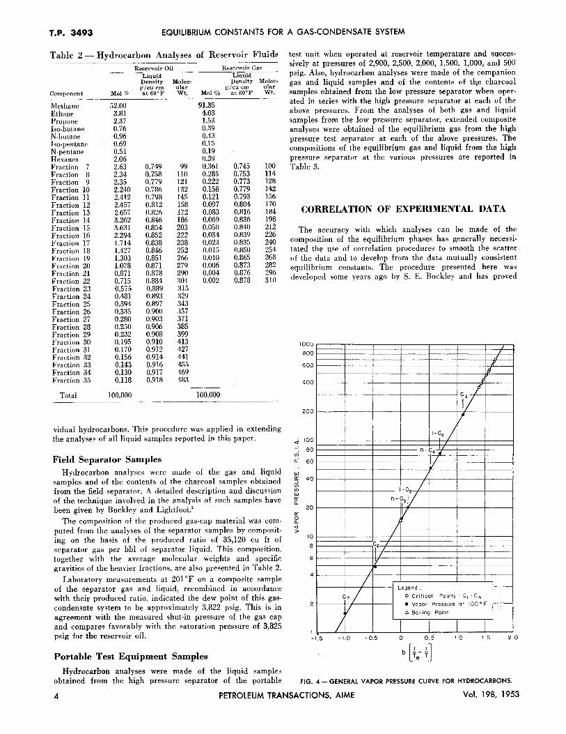
The accuracy with which analyses can be made of the composition of the equilibrium phases has generally necessi­tated the use of correlation procedures to smooth the scatter of the data and to develop from the data mutually consistent equilibrium constants. The procedure presented here was developed some years ago by S. E. Buckley and has proved

w D:'. ::> (fJ (fJ

w D:'. a.

D:'. 0 a. <! >

IOOU

800

600

400

200

100

80

60

40

20

10

8

6

4

2

I -1.5

c , 16 I

I/ y

J

I C1 I I

I - LO - 0.5

, , j

.P d

~

c /'

1/ I

1-c. /i , n-c4 ~' I

I I

1.:1 J

1-c5 / n-cs/J

v /

I I

,

I

Legend : --

O Critical Points C1 . Ca

• Vapor Pressure a~ 100°F ~

6 Boiling Point

0 0.5 1.0 15 2.0

b[.!._l] T8 T

FIG. 4 - GENERAL VAPOR PRESSURE CURVE FOR HYDROCARBONS.

4 PETROLEUM TRANSACTIONS, AIME Vol. 198, 1953

A. E. HOFFMANN, J. S. CRUMP AND C. R. HOCOTT T.P. 3493

Table 3 - Hydrocarbon Analyses of Test Samples ----------------- ----------·-- -·- --------------

SepJTator Temperature: 201°F Pressure: psig 2900 2500 2000 1500 1000 500

Gas Liquid Gas Liquid Gas Liquid Gas Liquid Gas Liquid Gas Liquid Component Mo!% Mo!% Mo!% Mol'/c Mo!% Mol o/r Mo! o/d Mol% Mol'/o Mo!% Mo!%' Mol%

------- ---- ----·-·-

Methane 91.65 46.45 92.05 41.16 92.18 34.19 92.00 27.32 91.89 19.55 92.09 10.43 Ethane 4.17 4.36 4.01 3.92 4.03 3.62 4.11 3.56 4.25 2.96 4.02 2.09 Propane 1.56 2.86 1.53 2.71 1.57 2.87 1.60 2.89 1.66 2.59 1.56 1.97 !so-butane 0.33 0.93 0.33 0.94 0.34 1.02 0.35 1.09 0.35 0.99 0.35 0.75 N-butane 0.47 1.25 0.43 1.32 0.44 1.55 0.46 1.70 0.46 1.66 0.44 1.30 Iso-pentane 0.16 0.90 0.18 1.04 0.15 0.97 0.16 1.09 0.16 0.98 0.14 0.65 N-pentane 0.19 0.65 0.17 0.67 0.17 1.06 0.19 1.15 0.19 1.20 0.20 1.15 Hexanes 0.38 3.14 0.37 3.07 0.33 3.65 0.37 4.50 0.37 4.47 0.36 4".24 Fraction 7 0.301 3.69 0.278 5.48 0.238 5.34 0.260 7.03 0.238 6.39 0.312 7.88 Fraction 8 0.228 3.81 0.218 5.08 0.191 6.09 0.213 7.32 0.183 8.27 0.235 9.29 Fraction 9 0.167 3.56 0.154 4.32 0.142 5.62 0.127 6.84 0.115 9.20 0.156 8.83 Fraction 10 0.119 3.099 0.101 4.035 0.089 5.242 0.069 6.211 0.063 8.927 0.073 8.553 Fraction 11 0.089 2.978 0.067 3.975 0.052 5.245 0.038 5.674 0.031 7.934 0,035 8.178 Fraction 12 0.061 3.085 0.043 4.071 0.030 :>.226 0.024 5.238 0.017 6.424 0.018 7.839 Fraction 13 0.045 3.557 0.026 4.673 0.019 4.971 0.015 5.182 0.010 5.177 0.009 7.603 Fraction 14 0.034 4.452 0.019 4.644 0.013 4.718 0.009 4.690 0.007 4.217 0.002 6.719 Fraction 15 0.022 3.302 0.015 3.156 0.009 3.133 0.005 3.081 0.004 3.067 4.519 Fraction 16 0.014 2.063 0.009 1.979 0.005 1.861 1.923 0.002 2.037 2.776 Fraction 17 0.010 1.453 1.364 0.002 1.249 1.064 1.327 1.813 Fraction 18 1.191 1.023 0.832 0.811 0.914 1.246 Fraction 19 1.001 0.718 5.583 0.629 0.642 0.857 Fraction 20 0.856 0.509 0 432 0.421 0.493 0.593 Fraction 21 0.742 0.143 0.307 0.350 0.316 0.372 Fraction 22 0.621 0.221 0.236 0.265 0.239 Fraction 23 0.113

Tot~l 100.00(J 100.000 100.000 100.000 100.000 100.000 100.000 100.000 100.000 100.000 100.000 100.000 . - ------·----------------- ------------- - ----- ---· - --------- ----- -

Table 4 - Values of b ( 2_ _ 2_) for 201°F T11 T

·------~-- -----·~---------- ------------· ---- ------------ - --------·~---------------·--- -TB T .. p"

Smoothed b ( 2_ _ :_) Boiling Critical Critical Point Temperature Pressure Values T T

Hydrocarbon 'R Tn 'R T,. psi a b* bt ]I

--------- -- -------------- ---·-------- ·-----Me·hane 201.01 0.0049749 343.3 0.0029129 673.1 805 805 2.786 Ethane 332.16 .0030106 549.77 .0018189 708.3 1,412 1,412 2.114 Propane 415.96 .0024041 665.95 .0015016 617.4 1,799 1,799 1.602 !so-butane 470.58 .0021250 734.65 .0013612 529.l 2,037 2,037 1.245 N-butane 490.79 .0020375 765.31 .0013067 550.7 2,153 2,153 1.128 Iso-pentane 541.82 .0018456 829.8 .0012051 48.3. 2,368 2,368 0.786 N-pentane 556.62 .0017966 845.60 .0011826 489.5 2,480 2.480 0.702 N-hexane 615.42 .0016249 914.1 .0010940 439.7 2,780 2,780 0.309 N-heptane 668.86 .0014951 972.31 .0010285 396.9 3,068 3,068 -0.057 N-octane 717.89 .0013930 1.024.9 .0009757 362.1 3,335 3,335 -0.402 N-nonane 763.12 .0013104 1,071. .0009337 331. 3,590 3,590 -0.729 N-decane 805.11 .0012421 1,114. .0008977 306. 3,828 3,828 -1.039 N-undecane 844.27 .0011845 1,152. .0008681 282. 4,055 4,055 -1.335 N-dodecane 880.99 .0011351 1,186. .0008432 263. 4,291 4,291 -1.624 N-tridecane 915.54 .0010923 1,219. .0008203 250. 4,524 4,500 -1.896 N-tetradecane 948.15 .0010547 1,251. .0007994 230. 4,678 4,715 -2.164 N-pentadecane 979.02 .0010214 1,278. .0007825 220. 4,919 4,919 -2.421 N-hexadecane 1,008.38 .0009917 1,305. .0007663 200. 5,030 5,105 -2.664 N-heptadecane l,036.30 .0009650 1,323. .0007559 190. 5,315 5,290 -2.902 N-octadecane 1,062.97 .0009408 1,350. .0007407 180. 5,440 5,470 -3.133 N-nonadecane 1,088.48 .0009187 1,368. .0007310 170. 5,664 5,630 -3.349 N-eicosane 1,112.91 .0008986 1,395. .0007169 160. 5,706 5,790 -3.561 N-heneicosane l,136.3t .0008801 5,945§ -3.766 N-docosane l,158.8t .0008630 6,095§ -3.965

-··------~~

(log Pc - log 14.7) *Comvuted from re]ation b == -~--

(_!_ _ _:_) TB T"

tValues of b for normal hydrocarbons smoothed by plot of b vs number of carbon atoms. tEstimated from extrapolation of boiling point data. §Estimated from extrapolation of plot of b vs number of carbon atoms. NOTE: Physical constants of hydrocarbons taken from publications released by API Research Project 44.

Vol. 198, 1953 PETROLEUM TRANSACTIONS, AIME 5

T.P. 3493 EQUILIBRIUM CONSTANTS FOR A GAS-CONDENSATE SYSTEM

Table 5-Smoothed Values of KP at 201°F

Condensate -------------------Gas-Oil System: --------------- ---------Pressure, psig:

Component

Methane Ethane Propane !so-butane N-butane Iso-pentane N-pentane Hexanes Fraction 7 Fraction 8 Fraction 9 Fraction 10 Fraction 11 Fraction 12 Fraction 13 Fraction 14 Fraction 15 Fraction 16 Fraction 17 Fraction 18 Fraction 19 Fraction 20 Fraction 21 1''raction 22

3;822

6,750 3,740 2,420 1,790 1,610 1,200 1,110

795 582 434 326 250 193 153 122 96.5 74.7 59.5 47.1 37.9 30.2 23.8 19.4 15.1

2,900

5,751 2,790 1,620 1,130

990 690 630 415 283 197 139 101 73.5 54.7 41.3 31.2 23.3 18.2 14.5

-------------- -------------·

2,600

- ----·-------5,623 2,510 1,375

907 790 525 472 298 192 128

87.0 60.3 42.6 30.7 22.3 16.4 11.9 9.05

very satisfactory. In this procedure, the data are smoothed by plotting for each hydrocarbon the log of the product KP (the equilibrium constant times the absolute pressure) against a

function b ( !__ - !__) , where b is a constant, characteristic Tn T

10,000 C2-= =c1--9• M

c. / --I /Al,,

5000

Cs I ,/. ~ I ,Y ~ r Reservoir Temperature· 201 • F. I ./ h IOOO

500

100 <( ::::=c20 ui 50 a: a.

I I

11) "" 10

5

5

J -4.0

,/

6 o, CIO ~ ./ /", y // "/ '-

I y' /o ,/ /

I I / /o /, ·; '/ c,. j

I I vv / /. . ' Vi 7//

0 , -. 9 / "/ /.-,

v / ./ / -.,, -~

/ / 0 , .v / I ,/ 0 /• / )' I

(2)/ v •/. ) '/ 7 . (3)

0 0/ 0 , , , L , ,

.,/ / I I ·-~

, ·/ /' .I (4)

(5) 0 / I " 0 J J, Pressure

Legend p.s.i.g. System (I) 3827 Gos -Oil , (2) 2900 Gos - Condensate

(6) / (3) 2500 " " (7) (4) 2000 " "

(5) 1500 " " (6) 1000 " " . (7) 500 " "

I

-3.0 -2.0 -1.0 . 0.0 1.0 2.0 3.0

b [-!._ ..!.._] T8 T

FIG. 5 - EXPERIMENTALLY DETERMINED K-VALUES AT 201°F.

2,000 1,500 1,000 500

KP: psia ---- --- --------- ---------

5,432 5,100 4,769 4,544 2,170 1,800 1,515 1,260 1,100 840 650 490

682 495 360 253 582 414 295 203 367 247 165 107 323 217 142 90.5 190 120 74.1 43.3 118 69.7 40.3 21.9 74.3 41.5 22.5 11.5 47.6 25.1 13.0 6.23 31.5 15.7 7.73 3.50 21.1 10.1 4.72 2.00 14.7 6.65 2.96 1.19 10.2 4.47 1.89 0.730 7.20 3.02 1.22 0.445 4.96 2.00 0.780 3.64 0.527 2.72

of the particular hydrocarbon, T 8 is its boiling point in °R, and T is the temperature in °R. It has been found empirically that for the equilibrium between a gas and a liquid at any given pressure, the logarithms of the KP products for the individual hydrocarbons so plotted yield reasonably straight

lines against the function b ( !__ - !__) . * In Fig. 5 the KP Tn T

products obtained from the experimental data are plotted against this function. On the whole, the relationship drawn to define the behavior of the KP products represents the experi­mental data well within the limits of reproducibility.

*The basis for this method of correlation is as follows:

1. There is an analogy between the product KP and the pure liquid vapor pressure of a dissolved component.3

2. The logarithms of the vapor pressures of pure substances when plotted against the reciprocal of the absolute temperature yield approxi­mately straight lines over reasonable temperature intervals.

3. The vapor pressures of pure hydrocarbons on a conventional Cox chart4 converge to a common point of intersection.

These facts have long been known. Although the Cox chart has a tem-

perature scale that differs slightly from _:_.the l:onvergence of the vapor-T

pressUl'e. lines suggests that they might be rotated into a single line by appropriate changes in slope, which can be dOne by employing a single constant for each line. This approach was ther~fore employed to construct

p a single ·vapor-pressure curve for all hydrocarbons by plotting log ~-

14.7

vs b ( _:_ - !. ) , wher7·-~·'. J~ the factor required for each hydrocarbon to T

11 T . ,,, ,

rotate its vapor .. pressure ··eurve to the commou line. This vapor-pressure curve is shown in Fig. 4. This single line was found to represent the vapor­pressures of hydrocarbops , with reasonable accuracy over a substantial temperature range. · 1 • • < .1

su::I::• :~Yt:::e::::r::::::::obm mt: :~:::nu:: f3: t:e(v!~rt)es~ P1 T, T,

Experience has indicated that values of b computed from the critical pres­sures and temperatures and the normal boiling points are satisfactory for correlation purposes for most condensate reservoirs. Values of b calculated in this manner for the various hydrocarbons are presented in Table 4. Values for the high .molecular weight hydrocarbons were deter­mined from a smooth curve of a plot of b va number of carbon atoms in the molecule.

The aforementioned analogy between KP and vapor pressure led then

to the correlation technique of plotting log KP vs b · ( ~ - 2_ ) for the . . TB T

various components of an equilibrium mixture of oil and gas.

6 PETROLEUM TRANSACTIONS, AIME Vol. 198, 1953

A. E. HOFFMANN, J. S. CRUMP AND C. R. HOCOTT T.P. 3493

Table 6 -Hydrocarbon Analysis of Upper Reservoir Gas

Liquid Density Molecular Component Mo!% g/cu cm at 60°F Weight

Methane 90.74 Ethane 4.35 Propane 1.69 !so-butane 0.36 N-butane 0.54 Iso-pentane 0.20 N-pentane 0.21 Hexanes 0.42 Fraction 7 0.419 0.741 100 Fraction 8 0.292 0.752 114 Fraction 9 0.245 0.770 128 Fraction 10 0.167 0.775 142 Fraction 11 0.116 0.783 156 Fraction 12 0.090 0.793 170 Fraction 13 0.067 0.807 184 Fraction 14 0.049 0.835 198 Fraction 15 0.028 0.837 212 Fraction 16 0.014 0.843 226 Fraction 17 0.003 0.847 240

Total 100.000

The smoothed values of KP taken from the above plot are presented in Table 5. These data are further presented in Fig. 6 as a cross plot of KP against pressure at reservoir tem­perature. Where possible, the data have been extended below 500 psig by extrapolation to the vapor pressures of the par­tic~lar hydrocarbons at 201°F.

SELECTION OF EQUILIBRIUM CONSTANTS FOR ANOTHER RESERVOIR

To determine the utility of the above correlation in develop­ing equilibrium constants for another gas-condensate system of similar composition, a second reservoir in the same. Southwest Texas field was selected for investigation. On a production test, this reservoir produced gas and condensate at a rate of 36,199 cu ft/bbl of separator liquid from a well completed at a depth of 6,200 to 6,205 ft subsea. During testing, the field separator was operating at a pressure of approximately 780 psig and a temperature of 73°F. The reservoir pressure and temperature were 3,117 psig and 189°F, respectively. The composition of the reservoir material was obtained from anal-

FIG. 6 - EFFECT OF PRESSURE ON K-VALUES AT 201°F.

yses of field separator gas and liquid samples in the same manner as that described above. This composite hydrocarbon analysis is presented in Table 6. A dew-point determination on a composite sample of separator gas and liquid recombined in accordance with their produced ratio was also made in the laboratory. This dew point was indicated to be approximately 3,117 psig, the reservoir pressure at the time of sampling.

In order to select equilibrium constants appropriate for this

reservoir, the function b ( ~-~) was computed for each Tn T

Table 7-Smoothed Values of KP at 189°F

Pressure, psig: 2,900 2;500 2,000 1,500 1,000 l11r·1

500 Component KP: psia

Methane 5,580 5,450 5,220 4,860 4,550 4,310 Ethane 2,690 2,410 2,070 1,715 1,430 l,190 Propane 1,540 1,290 1,030 782 595 447 !so-butane 1,055 845 630 455 325 228 N-butane 925 730 535 377 265 180 Iso-pentane 640 482 333 223 147 94.0 N-pentane 585 437 298 196 127 79.5 Hexanes 383 272 173 107 65.3 37.8 Fraction 7 258 175 105 61.5 35.0 18.7 Fraction 8 178 114 65.4 36.1 19.2 9.62 Fraction 9 125 77.0 41.7 21.7 11.l 5.20 Fraction 10 90.0 53.3 27.2 13.5 6.50 2.87 Fraction 11 65.0 37.2 18.0 8.60 3.90 1.61 Fraction 12 47.5 26.1 12.2 5.47 2.36 0.930 Fraction 13 35.4 18.8 8.35 3.59 1.48 0.555 Fraction 14 26.5 13.7 5.77 2.39 0.945 0.332 Fraction 15 20.l 10.0 4.08 1.61 0.610 0.204 Fraction 16 15.5 7.45 2.91 1.11 0.402 0.128 Fraction 17 11.9 5.60 2.10 0.770 0.269 0.0810

Vol. 198, 1953 PETROLEUM TRANSACTIONS, AIME 7

T.P. 3493 EQUILIBRIUM CONSTANTS FOR A GAS-CONDENSATE SYSTEM

10,000 - Q£r..Q£!!. Atoms l -

5000 -

2 -

,_.-- __.-er ~ 3 ---- - - l-o::>4 = 1000 >5 = ~ -

~ ~

-

~ -500 - - -- ~ -

- ---- ~ ~ ~ '~ ----- ~ L.--' L--:: ~ v ~ v 10

~ 100

- """ ~ -- - -- -50 --- ~ ~ ~ / ../ ""' 15 -

~ ~ ~- i,.......- / ~/ .//......-" <l

~ / /,,...... ~ ~ Y' <f)

a. 10

- ~ - - - - -- - - ,,; / -- ,/ - - - ,_

/ ../ / / ,, // \ a. 5

"' v / // // r/ \

/_/ // ~y Reservoir Press .3117_1,

.· / - / 5 ,' ·' '!' /

I / / / ' / / / I/ I Reservoir Temperature 189° F

, -- ~- ~-~ , , , . -l I

I

I J

05

1000 2000 3900 PRESSURE : P S. I G.

FIG. 7 - EFFECT OF PRESSURE ON K-VALUES AT 189°F.

c(>mponent o(the system at a temperature of 189°F, the reser­voir temperature. Then, using the graph in Fig. 5, KP products for each hydrocarbon were determined at the corresponding

b ( 2__ _ 2__) from the curves at the various pressures. These Tn T

KP products are presented in Table 7. These data are illus­trated in Fig. 7 in a plot of KP against pressure for each component of this particular hydrocarbon system. The points indicated on the graph at each pressure are those determined from Fig. 5 for that pressure.

At pressures above 2,500 psig the curves were extended to 3,117 psig by trial and error in such a manner as to satisfy dew-po,f_r;it. conditions. The differences between the extended curves and the points shown at 2,900 psig indicate the adjust­ment in the smoothed experimental data required for applica­tion to the re~ervoir fluids in the second reservoir. The extent of this deviation is such that no adjustment appears necessary at pressures lower than 2,500 psig, and the corresponding equilibrium constants should be satisfactory for computations of the phase behavior of this gas-condensate system.

Although calculations made with equilibrium constants correlated in this manner have not been checked by following the actUal depletion of a gas-condensate reservoir, comparisons of su~h computations with depletion-type experiments on recombined samples in the laboratory have yielded results that appeared to be entirely adequate.

It should be pointed out that the method of correlation pre­sented here is designed solely for the correlation of equilib­rium constants for a particular system. Since it is well known that equilibrium constants, particularly at high pressure, are

quite sensitive to composition, it is obvious that the particular equilibrium constants presented in this paper would not be applicable to another gas-condensate system of substantially different composition. In no sense are they offered as being generally applicable. The method of correlation, however, as distinct from the particular equilibrium constants, is one that has been found useful for many gas-condensate systems cover­ing a wide range of composition. For each system experimental data are required for that particular system. For the smoothing of and detection of errors in analyses of equilibrium mixtures, the method has been rather rigorously tested. The limits to which the method can be employed to extend equilibrium con­stants for a particular system into regions of temperature and pressure beyond those experimentally employed have not been fully determined.

REFERENCES

1. Buckley, S. E., and Lightfoot, ] . H.: "Effects of Pressure and Temperature on Condensation of Distillate from Nat­ural Gas," Trans. AIME, (1941), 142, 232.

2. Flaitz, ]. M., and Parks, A. S.: "Sampling Gas-Condensate Wells," Trans. AIME, (1942), 146, 13.

3. Nysewander, C. N., Sage, B. H., and Lacey, W. N.: "The Propane-n-Butane System in the Critical Region," lnd. and Eng. Chem., (1940), 32, (1), 118.

4. Cox, Edwin R.: "Pressure-Temperature Chart for Hydro­carbon Vapors," lnd. and En{(. Chem., (1923), 15, (6),

592. * * *

DISCUSSION

By Fred H. Poettmann, Phillips Petroleum Co., Bartlesville, Okla., Junior Member AIME

The authors have made an excellent contribution by making available equilibrium data at reservoir conditions of the high boiling hydrocarbon fractions in a gas-condensate system. It is the high boiling hydrocarbon fractions which have the greatest effect in calculating the dew point of a gas condensate system, and the more information we have on these fractions, the more accurate will be our predictions. The procedure used by the authors for obtaining equilibrium vaporization ratios for the high boiling fractions is very good.

We shall divide our discussion of the authors' correlation procedure into two parts, (1) the origin of the correlation, and (2) the authors' application of the correlation.

The relationships used by the authors in correlating their equilibrium vaporization ratios can be found in any good text on thermodynamics. Equation ( 1) can be derived assuming only ideal solutions in the vapor and liquid phases.

where

lnK = b' ---( 1 l )

b' = 6H R

Tn T

;:,.H = heat of solution of component R = gas constant

(I)

T., = normal boiling point of component m degree,, Rankine

T = equilibrium temperature degrees Rankine

The relationship used in Equation (2) is that employed by the authors. In addition to the assumption of ideal solutions

8 PETROLEUM TRANSACTIONS, AIME Vol. 198, 1953

A. E. HOFFMANN, J. S. CRUMP AND C. R. HOCOTT T.P. 3493

KP- PSIA

100.0

10.0

1.0

0.1

'f - 800°F

e - 500°F

• -100 °F

NORMAL BOILING POINT RANGE

300°F TO 900°F

0.01-~~~~-'--'--'--'---'---'--'---'--'--' 3.0 2.0 1.0 0 1.0 2.0 3.0 4.0

b[+e-+J

10,000

1,000

KP- PSI A

100

10 e- 250°F

A- 50°F

l...__.___.__,__.__.__,___,___.._L-J...-..l.--'--....i.._J

3.0 2.0 1.0 0 1.0 2.0 3.0 4.0

b[J__..Ll Te Tj

FIG. I - EQUILIBRIUM VAPORIZATION RATIOS, HIGH BOILING HYDRO- FIG. 2 - EQUILIBRIUM VAPORIZATION RATIOS, C1 TO c,. ROLAND, CARBON FRACTIONS. CHARACTERIZATION FACTOR 10.5. SMITH AND KAVELER.

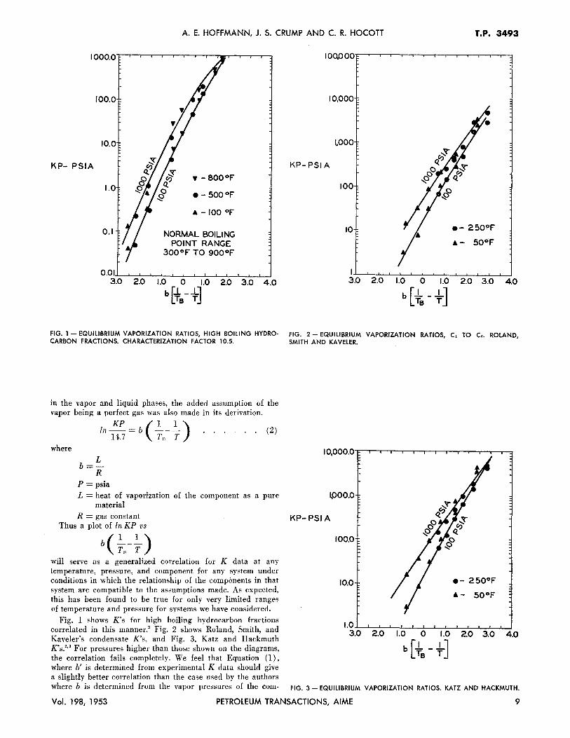
in the vapor and liquid phases, the added assumption of the vapor being a perfect gas was also made in its derivation.

where

Zn--= b ---KP (1 1)

L b=­

R P = psia

14.7 TB T (2)

L = heat of vaporization of the component as a pure material

R = gas constant Thus a plot of Zn KP vs

b( ~-~) TB T

will serve as a generalized correlation for K data at any temperature, pressure, and component for any system under conditions in which the relationship of the components in that system are compatible to the assumptions made. As expected, this has been found to be true for only very limited ranges of temperature and pressure for systems we have considered.

Fig. 1 shows K's for high boiling hydrocarbon fractions correlated in this manner.' Fig. 2 shows Roland, Smith, and Kaveler's condensate K's, and Fig. 3, Katz and Hackmuth K's."' For pressures higher than those shown on the diagrams, the correlation fails completely. We feel that Equation (1), where b' is determined from experimental K data should give a slightly better correlation than the case used by the authors where b is determined from the vapor pressures of the com-

~000.0

KP-PSI A

100.0

10.0 e- 250°F

4- 50°F

1.0-'::"----'-::~~-'---'---'---'---'--'---'---'---'---'--' 3.0 2.0 1.0 0 1.0 2.0 3.0 4.0

b [J_ _ l_J Te T

FIG. 3 - EQUILIBRIUM VAPORIZATION RATIOS. KATZ AND HACKMUTH.

Vol. 198, 1953 PETROLEUM TRANSACTIONS, AIME 9

T.P. 3493 EQUILIBRIUM CONSTANTS FOR A GAS-CONDENSATE SYSTEM

KP-PSIA

6,000

1,000 2900 PSIG

100

10 • 0 200 400 600 800 I 000 1200 1400

NORMAL BOILING POINT (Te) - 0 R

FIG. 4 - EQUILIBRIUM VAPORIZATION RATIOS VS NORMAL BOILING POINT OF COMPONENT. TEMPERATURE, 201°F.

ponents in the pure state. In neither case, will the K data correlate in the range of high temperatures and pressures which include retrograde behavior.

In the application of the correlation, the authors first justify the use of the correlation as a means of smoothing their experi­mental data. The authors' Fig. 5 is restricted to a constant temperature, the reservoir temperature. The variables on this plot are K, P, and T n, b is not an independent variable, hut a function of T n, only. The petroleum industry has for years correlated K's at constant temperature by simply plotting Zn K or Zn KP vs the normal boiling point for lines of con­stant pressure. Fig. 4 is a plot of three of the constant pres­sure lines shown on the authors' Fig. 5. The curves are identi­cal to those shown on the authors' Fig. 5. The experimental data are also indicated. We cannot see any advantage of using the authors' correlation as a means of smoothing K data at constant temperature.

In extending equilibrium vaporization ratios to another temperature, the authors actually use the correlation as a general method for obtaining K data. This procedure will give reasonable results at low pressures and temperatures but, as stated previously, at high temperatures and pressures, and especially in the region of retrograde behavior, the K data will not correlate. The authors warn that the procedure should not he applied to widely different conditions of temperature and composition. This warning is well taken. Fig. 5 gives an indi­cation of what can occur if the temperature variation alone is too large. It is a plot of

lnKPvs b ( !__!_) Tn T

at 3,000 psia and 150, 201, and 250°F. The data were obtained from the condensate system of Roland, Smith, and Kaveler.' Fig. 5 shows that the K data do not correlate as a single curve at 3,000 psia and 150, 201, and 250°F. Tabulated below are the differences in the actual values of Kat 250°F and K values at 250°F adjusted from the 201 °F curve, all taken at 3,000 psia. Only K values of methane through pentane were compared.

Km Adjusted from K,,o K,,o Per Cent

Component 201°F Actual Deviation Deviation

c, 2.10 2.02 +0.08 + 3.96 c, 1.14 1.04 +0.10 + 9.62 C, .73 0.62 +0.11 +17.7 c. .49 0.40 +0.09 +22.5 c, .37 0.30 +om +23.3

As can be seen, the higher the boiling point, the greater the percentage deviation in the K value.

REFERENCES

1. Poettmann, F. H., and Mayland, B. J.: "Equilibrium Con­stants for High Boiling Hydrocarbon Fractions of Varying Characterization Factors," Petroleum Refiner, (July, 1949), 28, (7)' 101.

2. Roland, C. H., Smith, D. E., and Kaveler, H. H.: "Equi­librium Constants for a Gas-Distillate System," Oil and Gas four., (1941), 39, ( 46), 128.

3. Katz, D. L., and Hackmuth, K. H.: "Vaporization Equilib­rium Constants in Crude Oil - Natural Gas System," Ind. and Eng. Chem., (1937), 29, 1072. * * *

7000 C1 6000

5000

4000 P= 3000 PSIA

3000

2000

KP- PSIA C4

1000 900 800 700

1.0 1.5 2.0 2.5 3.0 3.5 b[.L-.L] Te T

FIG. 5 - EFFECT OF TEMPERATURE ON CORRELATION. ROLAND, SMITH AND KAVELER K DATA.2

10 PETROLEUM TRANSACTIONS, AIME Vol. 198, 1953