Equilibrium Tax Rates and Income Redistribution:A Laboratory Study1

Marina Agranov2 and Thomas R. Palfrey3

This Version: April 2, 2013Preliminary and Incomplete.

1The financial support of the National Science Foundation (SES-0962802) and the Gor-don and Betty Moore Foundation is gratefully acknowledged. We are grateful for commentsfrom seminar audiences at Caltech, The BCEP Workshop in Berkeley, the LABEL Inau-guration Conference at USC, and John Londregan.

2Division of the Humanities and Social Sciences, California Institute of Technology, MailCode 228-77, Pasadena, CA 91125. Email: magranov@hss.caltech.edu.

3Division of the Humanities and Social Sciences, California Institute of Technology, MailCode 228-77, Pasadena, CA 91125. Email: trp@hss.caltech.edu.

Abstract

This paper reports results from a laboratory experiment that investigates the Meltzer-Richard model of equilibrium tax rates, income redistribution, and the growth ofgovernment.

1 Introduction

In the US and other democratic countries, taxes are decided by the political process,and income tax policy especially has enormous consequences for the economy, bothin terms of the distribution of income and inequality as well as economic efficiency.On one hand, income taxes are used to finance public expenditures on governmentservices that are at least partly redistributive in nature, such as public education,public insurance and social programs. These expenditures are aimed at benefitingsociety as a whole, but the costs of these programs are borne in proportion to income(or, under progressive taxation, more than proportionally to income). On the otherhand, taxes may negatively affect efficiency of the economy through distortions inthe private sector. In fact, this fundamental tradeoff between the level of incometaxes (and hence the amount of redistribution) and the functioning of the economyis the main dimension of political conflict and polarization over tax policy that hascome to dominate electoral and legislative politics on economic issues.

Theoretical literature in the 1970s has proposed a rigorous, equilibrium-based politi-cal economy approach to addressing the positive question of how the level of incometaxes are determined in the democratic society (see Romer (1975), Roberts (1977)and Meltzer and Richard (1981)). The efficiency-equity tradeoff in these models iscaptured by a distortion to labor supply created by a gap between the after-tax wageand a workers marginal productivity. The heterogeneity in the agents’ productivitiesis the driving force behind inequality in the pre-tax incomes. While predictions ofthese models have enormous consequences for the economy, both in terms of inequal-ity level and economic efficiency, implications of these theories are extremely difficultto test using macro field and historical data sets, for which there are relatively lim-ited time series available. There are open methodological issues about the extentto which these studies enable one to draw causal conclusions, as well as the deeperproblem of endogeneity of the economic and political variables using historical orcontemporary data. There have been several attempts, but taken collectively, thesestudies have led to ambiguous (and sometimes conflicting) conclusions.1

1Several papers attempted to test the median voter tax hypothesis, which is implied by modelsmentioned above and suggests that the tax rate and/or government expenditures in democracieswill correspond to the ideal level of public expenditure of the median voter. Meltzer and Richard(1983) test this with data on their categorization of redistributive expenditures in the U.S. between1936 and 1977, but exclude expenditures on public goods such as public safety, defense, and in-frastructure. They dont find direct evidence for the hypothesis, but find that purely redistributiveexpenditures are positively correlated with the ratio of mean to median income. Milanovic (2000),in a cross-sectional study of 24 democracies, also finds that factor income redistribution to the poor

1

In spite of the inconclusive empirical evidence, there is a widespread consensus aboutinterdependence between agents’ behavior in economical and political domains. In-deed, labor supply crucially depends on the amount of taxation imposed by the po-litical process and, vice-versa, indirect preferences of agents for the level of taxationand redistribution crucially depend upon agents’ beliefs about labor market behaviorof other agent. For instance, poor may prefer a lower tax rates if they have reasonto believe that rich might withhold labor when taxes are too high. While theoreticalliterature has long recognized the necessity to study the interplay between marketbehavior of heterogeneous agents and their preferences for redistribution expressedin the political arena, existing experimental literature lags behind (see Section 1.1for the literature review).2

Our paper aims to fill this void. In our experiment subjects operate in two envi-ronments: political environment, in which the level of taxation is determined, andthe labor market (economical environment), in which given the level of redistributionand the assigned productivities citizens choose labor supply that generates pre-tax in-come. Because of the redistributive effect of income taxation and because individualsdiffer in their productivities and hence their incomes, individuals in our experimenthave different indirect preferences for the level of taxation and these preferences de-pend upon the distribution of productivities in the economy. Political institutionsare the means by which these heterogeneous preferences are aggregated into a publicdecision on the tax rate. However, because the tax rate in turn affects the amountof income that is generated by the private economy, agents preferences for redistri-bution themselves are endogenous and depend on how taxes affect individual laborsupply decisions.

Our experimental design is motivated by two main goals and it integrates ideas fromeconomic experiments on labor supply, voting experiments and experiments on can-didate competition in elections. The first goal is to provides a direct test of Meltzer

correlates with measures of income inequality, but finds little support for the median voter hypoth-esis. On the other hand, Perotti (1996), in his cross-sectional study of 67 countries, does not findsignificant evidence for a positive relationship between inequality and middle class tax rates. Thus,the overall picture is one of mixed empirical findings. While some of the findings are suggestiveof a link that would be consistent with the median voter tax hypothesis, the link is tenuous anddoes not help identify the mechanism by which the median voters preferences are revealed in thepolitical process.

2The noticeable exception is recent study of Grosser and Reuben (2013) which we discuss indetails in Section 1.1.

2

and Richards (1981) model and study the political economy equilibrium that emergesunder two different majoritarian political processes: direct democracy and represen-tative democracy. In the direct democracy mechanism, the median voter’s preferredpolicy is elicited directly, while in the representative democracy mechanism voterschoose in an election between two office-motivated candidates who compete by choos-ing tax rates as their platforms.3 The second exercise is to study the link betweeninequality and redistribution. To do that we fix the political environment, vary theinequality level by varying the initial productivities of the citizens and test whetherhigher inequality leads to higher levels of taxation for a given political institution.

We have several main results. First, higher inequality leads to more income redis-tribution through higher taxation in both political regimes (direct democracy andrepresentative democracy). Second, both regimes implement on average theoreticallypredicted tax rates. Third, labor supply decisions of agents are very close to the op-timal with the exception that high income agents undersupply their labor especiallyfor the high tax rates. Finally, we observe a lot of heterogeneity in the implementedtaxes across different groups and this variation does not appear to be connected tothe variation of empirical labor supply functions across groups.

We see experiments as valuable component of the research agenda that aims at ad-vancing our understanding of the political economy of redistribution and taxation.Indeed, these controlled laboratory experiments provide a clean test of the theoret-ical models in very simple environments, while preserving the main incentives andtrade-offs that people face outside of the laboratory. Hence, data created from a care-fully controlled setting that can be used toward the development of better models.With respect to income redistribution, perhaps the most obvious candidate to be animportant behavioral factor would be other-regarding preferences (see Section XX).Further, our paper can be seen as one of the first attempts to study the interactionbetween labor market and political behavior, while keeping all the remaining details(political institution and distribution of productivities) constant and varying oneparameter at a time. For these purposes, experiments have a significant advantageover empirical research using historical time-series or cross-sectional data.

3One of the shortcomings of most theoretical models of the political economy of income taxationis that they are completely silent about the mechanics of the political process by which a tax rate ischosen. The models simply assume that under majority rule the tax rate preferred by the medianvoter would emerge, as if by magic. However recent work in political economics indicates that ainstitutional details of a democratic system cannot be ignored, as they may lead to a variety ofdifferent outcomes that do not correspond to the ideal point of the median voter.

3

The paper is structured as follows. In the remainder of this section, we discuss relatedliterature. Section 2 presents theoretical model which would serve as the basis forour experiments. Section 3 discusses in details experimental design. Results arepresented in Section 4 and Section 5 offers some conclusions. All the instructions forthe experiments are presented in Appendix.

1.1 Related Literature

Existing experimental literature has devoted a lot of attention to measuring pref-erences for redistribution. Some papers concentrate entirely on examination of twomotives - self-interest versus fairness - and abstract away from efficiency concern4.Others more recent studies investigate whether and how efficiency affects partici-pants’ social preferences by exogenously varying the size of the total pie to be dis-tributed and (in)equality of the shares. Bolton and Ockenfels (2002) conduct a seriesof voting games, in which subjects are confronted with two distributions of incomes- one that promotes efficiency and one that promotes equity. Tyran and Sausgruber(2006) report that social preferences of the Fehr-Schmidt type may explain votingbehavior on redistribution in an experiment where subjects were endowed with dif-ferent income levels and vote on a fixed amount of redistribution. Hochtl, Tyranand Sausgruber (2012) report a followup experiment suggesting that the ability ofinequality aversion to explain voting behavior on redistribution depends heavily onthe pre-tax distribution of income. In all papers described above, the amount of re-sources to be distributed is fixed exogenously and participants can only decide howto reallocate this surplus between themselves. In our experiments subjects’ labormarket decisions determine the total surplus generated. Moreover, while measuringpreferences for redistribution is not the main focus of our paper, our design allowsus to detect the presence of social preferences through analyzing both labor marketdecisions of agents as well as their voting patterns.

There are two recent studies that are closely related to our paper. Durante andPutterman (2009) conduct a laboratory experiment to study how preferences for re-distribution vary with fairness preferences, risk aversion, self-interest and the sourceof pre-tax inequality. In particular, the authors investigate whether preferences forredistribution are affected by (1) the way the distribution of pre-tax endowments aredetermined: randomly (by luck) or based on the score obtained in the unrelated task

4See Fehr-Schmidt (1999), Bolton and Ockenfels (2000), Rabin (1993), Andreoni and Miller(2002) and Fisman et al. (2007) for experimental work that studies dictator games

4

(such as SAT quiz or TETRIS game) and (2) whether the person choosing level ofredistribution is affected by this redistribution process him/herself or is merely a dis-interested observer. Among other things, the authors document that most subjectsprefer a more equal distribution of final wealth; however, this preference for highredistribution decreases substantially when the initial distribution of endowmentsis determined based on the task performance rather than randomly. Similarly tothe discussed above literature, the main goal of Duarnte and Putterman study is tomeasure subjects’ preferences for redistribution and how they are affected by variousfactors. Consistent with this goal, the authors use random dictator method to elicitsubjects’ preferences and abstract away from the details of political process that de-termine taxation level as well as strategic behavior of subjects in the political sphere,which is what we do in our study. Put differently, our focus is on the equilibriumbehavior of agents in both economical and political markets and how this behavioris affected by various political institutions used to determine taxes in the democraticsocieties.

The second closely related paper is that of Grosser and Reuben (2013), in which theauthors report the results of two laboratory experiments. In the first experiment,subjects first earn their income by trading in a double auction knowing that after thetrading is over their earned incomes will be subject to exogenously imposed redistri-bution (either zero or full redistribution). The goal of this experiment is to assessthe effect of redistribution on trading efficiency. The second experiment investigatesendogenous redistribution by introducing competition between two office-orientedcandidates who propose the level of redistribution just like in our study. However,in Grosser and Reuben, trading occurs before sellers and buyers know what tax ratewould be imposed on their earned incomes. In other words, agents operating in themarket need to form beliefs regarding the tax rate that would emerge from the candi-date competition and adjust their market behavior accordingly. On the contrary, inour experiments the tax rates are determined before agents choose their labor marketsupply, which allows us to study how taxes affect labor market decisions directly andnot through the belief channel.

We are aware of only one experiment that investigates the MR model: Konrad andMorath (2010). The main difference between Konrad and Morath and our paperis that in the former the experiment looks at individual choice behavior withoutany strategic interaction. Each subject plays against two computers that have pro-grammed behavior. Thus it does not test the equilibrium questions that are central tothe theory we are interested in our paper. In contrast, the experiment reported here

5

employs a design where workers/voters with heterogeneous productivities engagein multiplayer strategic interaction in both the political and economical domains.Furthermore, Konrad and Morath (2010) focus on different questions about the rela-tionship between social mobility and redistributive taxation, which we abstract awayin the current paper.

2 The Model

The economy consists of n > 1 agents. Agents operate in an perfectly competitiveand frictionless labor market and also participate in a democratic political processthat determines taxes which in turn affect labor decisions. We start by discussing thedecision problem of an agent in the labor market assuming that the tax rate is fixed,and then turn our attention to how political process shapes tax rates. To simplifyexposition, we describe here the setup with the utility function we implement in theexperiments. We refer readers to MR for the derivation of equilibrium with generalutility functions.

The Labor Market

Agent i is endowed with productivity wi. Individuals are identical in all other re-spects. The difference in choice of labor and consumption arise solely because ofthe differences in productivity. An agent with productivity wi that works xi timeunits earns pre-tax income yi = wixi and bears an effort cost of 1

2x2i which represents

the tradeoff between labor and leisure. Income and costs are measured in units ofconsumption and we assume no savings. In addition, an agent pays fraction t ofearned income in taxes. Tax revenues are redistributed in equal shares.5 So, utilityUi of agent i consists of three parts: after-tax disposable income, costs of labor andtheir share of redistributed taxes, where the latter depends on the entire profile of

5Equivalently, taxes are used to finance a level of public good,

y =1

n

n∑j=1

t · wjxj

and all agents value the public good according to the function V (y) = y, corresponding to the lastterm of equation (1).

6

productivities, w = (w1, ..., wn) and labor supply decisions x = (x1, ..., xn) :

Ui(wi, xi, t) = (1− t) · wixi −1

2x2i +

1

n

n∑j=1

t · wjxj (1)

Given the tax rate t, agent i chooses labor supply xi that maximizes the utility above,taking x−i as given. The utility function is concave, and the unique optimal laborsupply for individual i characterized by the first order condition:

x∗i (wi, t) =

(1− n− 1

nt

)wi (2)

Thus, all productive agents (i.e., wi > 0) have positive labor supply for all tax rates,t ∈ [0, 1]. Labor supply is declining in the tax rate and is proportional to a worker’sproductivity. Hence, pre-tax income is proportional to the square of productivity.Note that because of the additively separable specification of utilities, optimal laborsupply in our model does not depend on the labor supply decisions of other agentsin the economy.

The Political Process

Tax rates are determined by a political process. There are many possible voting rulesranging from dictatorship to unanimous consent, and each may produce a differentoutcome. In this paper, we focus on the majority voting rule, which is common inmany political situations. We start by describing the preferences of agents over taxrates and then derive the tax rate that emerges from the majority voting rule. Theutility of agent i when the tax rate t is implemented and all other agents follow thebehavior prescribed by the equilibrium in the labor market is:

U?i (wi, t) =

1

2

((1− t)2 − t2

n2

)w2

i +t

n

(1− n− 1

nt

)Z (3)

where Z =∑j

w2j denotes the aggregate income of the economy if the tax rate is t = 0.

PROPOSITION 1:

Agents’ preferences over tax rates satisfy three following properties:

7

1. Single-peakedness: for any wi, there exists t?i ∈ [0, 1] such that

U?i (wi, t) < U?

i (wi, t′) for all t < t′ ≤ t?i

U?i (wi, t) < U?

i (wi, t′) for all t?i ≥ t′ > t

2. Ideal points are ordered by productivity:

t?i ≤ t?j ⇔ wi > wj

3. The median ideal tax rate, t?m, is given by:

t?m =

[n2

n2−1 ·1nZ−w2

m2

n+1Z−w2

mif w2

m ≤ 1nZ

0 if w2m > 1

nZ

(4)

Proof : Single-peakedness is established in two steps. Clearly, ifd2U?

i (wi,t)

dt2< 0 in

the region t ∈ [0, 1], then single peakedness in the policy space follows immediately.From 3, we get:

dU?i (wi, t)

dt= −w2

i

(1− t+

t

n2

)+

1

nZ

(1− 2

n− 1

nt

)(5)

d2U?i (wi, t)

dt2=

n− 1

n2

((n+ 1)w2

i − 2Z)

(6)

Thus, single-peakedness is guaranteed by concavity of U?i for all individuals whose

productivity is sufficiently low, specifically if w2i <

2n+1

Z, i.e., as long as i’s zero-tax income is less than the average zero-tax income in the society. For relativelyhigh productivity workers, who do not satisfy this inequality, U?

i is convex, ratherthan concave. However, by solving for the tax rate, t∗i that satisfies i’s first ordercondition, (5), we get:

t∗i =n2

n2 − 1·

1nZ − w2

i2

n+1Z − w2

i

(7)

When 0 ≤ w2i <

1nZ, then concavity holds and the expression above characterizes i’s

ideal tax rate. When i’s productivity is in a slightly higher range, w2i ∈

[1nZ, 2

n+1Z],

then concavity continues to hold, and i’s ideal tax rate equals 0, since the value oft∗i given by (7) is negative, which is infeasible. Finally, for even higher productivity

individuals, such that w2i >

2n+1

Z, it is easy to show thatdU?

i (wi,t)

dt< 0 for all values

of t ∈ [0, 1]:

−w2i

(1− t+

t

n2

)+

1

nZ

(1− 2

n− 1

nt

)< 0⇔ w2

i > Z · n(1− 2t) + 2t

n2(1− t) + t

8

The last inequality holds true for w2i >

2n+1

Z since 2n+1

> n(1−2t)+2tn2(1−t)+t

.The second and third properties follow immediately. QED

The intuition for this characterization is straightforward. Agents with lower pro-ductivity prefer higher taxes, because they enjoy substantial redistributive benefitswhich for the most part come from the tax payments of the higher productivity,and hence higher income, agents. In contrast, agents with higher productivity preferlower taxes (or no taxes at all), because they end up subsidizing the large portion ofthe tax revenues from which they receive back only a small part in benefits.6

Single-peakedness and monotonicity of optimal tax with respect to productivitiescombined with the majority rule guarantee that the agent with the median produc-tivity (median voter) is decisive. Put differently, the tax rate, which is the mostpreferred by the median voter, is the only tax rate which beats any other tax rate ina pairwise competition, and is therefore a Condorcet winner. This result echoes themedian voter theorem from the spatial models of electoral competition.

Thus, the tax rate that emerges in a society that uses majority voting rule is t?m:

t?m =

[n2

n2−1 ·1nZ−w2

m2

n+1Z−w2

mif w2

m ≤ 1nZ

0 if w2m > 1

nZ

Total income in equilibrium is:7

n∑i=1

U∗i (wi, t) =1

2

(1− (n− 1)2

n2t2) n∑

i=1

w2i

One natural question that arises in this setup is how do tax rates compare acrosseconomies that differ in the distribution of productivity levels of its agents. Thefollowing corollary to Proposition 1 provides an answer to this question.

6These two properties are central in the theoretical literature that studies the political economyof redistributive taxation. Romer (1977) assumes that agents have Cobb-Douglas preferences overconsumption and leisure and derives conditions under which the preferences of agents are single-peaked in the tax rate. Roberts (1977) derives a more general condition that guarantees that idealpoints are inversely ordered by income. Meltzer and Richard (1981) assume the regularity conditionof Roberts (1977).

7The tax rate that maximizes total income is t = 0.

9

Corollary. Consider two economies with n individuals, which differ only in theprofile of productivities: wA in economy A and wB in economy B, and suppose thatwA

m = wBm . Then,

t?A = t?B = 0 if and only if w2m > 1

nZA > 1

nZB

t?A > t?B = 0 if and only if 1nZA > w2

m > 1nZB

t?A > t?B > 0 if and only if 1nZA > 1

nZB > w2

m

The corollary can be interpreted in terms of inequality in productivities as measuredapproximately by the variance of worker productivities. To see this, notice that inthe special case where the median productivity equals the mean productivity, then1nZ is approximately equal to the variance of wi, with the approximation being ar-

bitrarily close for large n. In this case, an increase in the variance that leaves themean unchanged will lead to a higher equilibrium tax rate. The tax rate chosen bythe median voter will be higher in the economy in which the productivity levels aremore unequal as captured by this variance-related measure, 1

nZ.

Also, if the distribution of productivities in economy A is more right skewed than theone in economy B then 1

nZA > 1

nZB and we would expect (weakly) higher taxes in

economy A than in economy B. The intuition for this result comes from the fact thattax revenues are rebated back to all agents in equal shares. When higher productivityagents become more productive, they work more and, thus, contribute more to thetotal tax revenues. Therefore, the median voter would prefer higher taxes and moreredistribution since an increase in the tax rebate associated with an increase in taxrates overweighs the decrease in after-tax disposable income.

3 Experimental Design

The experiment is designed to examine the comparative statics implied by the equi-librium tax rates and labor supply in the theoretical model described in Section 2,and to examine the robustness of these outcomes to the political institution. Beforewe launch into the details of the experimental design, recall that theory is silentabout the mechanics of the political process by which a tax rate is chosen. Indeed,the model simply assumes that under majority rule the tax rate preferred by themedian voter would somehow emerge, as if by an invisible (political) hand. However,empirical work suggests that institutional details of a democratic system may leadto outcomes that do not correspond exactly to the ideal point of the median voter.In fact, there is also considerable theoretical work demonstrating the plausibility of

10

non-median outcomes even with highly competitive democratic process. For exam-ple, competition between two purely office-motivated candidates on one dimension,and Euclidean preferences of voters, imply equilibrium policies at the mean voterideal point if voting is probabilistic. (Hinich 1977, Ledyard 1984, Coughlin 1992).Potential entry of third parties, proportional representation with multiple parties,and many other variations in the democratic institutions could, in principle, alsolead to non-median outcomes. Considerations like this lead us to design our ex-periment in a way that may allow us to reach some initial conclusions about therobustness of the MR theory of median voter tax rates to variations the democraticinstitutions.

With this in mind, our design considers two very different competitive democraticinstitutions for determining the tax rate. In a world with perfect information anperfect optimization by all agents, both regimes theoretically will produce the sametax rate outcome, which will correspond to the median voter ideal point. The twoinstitutions we consider are direct democracy and representative democracy.

Direct democracy (DD) is implemented by simply allowing every individual voter anequal say in the outcome, without introducing candidates or representatives. Underthe direct democracy mechanism, each voter proposes a tax rate, and the medianproposal is directly implemented. It is well known (Moulin 1985) that under thismechanism every voter has a dominant strategy to propose his or her ideal tax rate.Because it is a dominant strategy, as long as voters have rational expectations abouthow the tax rate affects the labor supply decisions of the other voters, then thisshould lead unambiguously to tax rate outcomes corresponding to equation 4, with-out any additional assumptions about information or beliefs held by the players inthe game.

Representative democracy (RD) is implemented as Downsian candidate competition,by introducing two additional players into the game, both of whom are purely of-fice motivated candidates, with no private preferences over tax rates. This leads toa three stage game. In the first stage, the two candidates simultaneously propose(binding) tax rates, which they will impose if they are elected to represent the vot-ers. In the second stage, voters simultaneously vote for one of the two candidatesfor representative, with no abstention. In the third stage, after the representative iselected, the voters make their labor supply decisions, taking as given the tax rate ofthe winning candidate. In this regime, if candidate have rational expectations abouthow each voter will vote between every pair of proposed tax rates, and in addition

11

voters have rational expectations about how tax rates affect labor supply decisions,then the unique subgame perfect Nash equilibrium is for both candidates to proposethe ideal tax rate of the median voter.

According to theory, the median voter’s ideal tax rate is the equilibrium in bothregimes. However, the informational requirements for the equilibrium are more dif-ficult to achieve in the RD regime. Not only must voters have rational expectationsabout labor supply distortions, but in addition the candidates must also have ratio-nal expectations about how voters choose between tax rates. In contrast, in the firststage of the DD regime, each voter has a dominant strategy to propose his or herideal tax rate, regardless of their beliefs about the proposal strategies of the othervoters. Thus, a priori, the RD regime, which more closely resembles a democraticprocess we observe, provides a tougher test for the theory.

In addition to questions about the effect of institutions on the tax rate, we alsowanted our design to address the basic question that originally motivated the theo-retical papers on equilibrium tax rates. Will a more unequal distribution of incomelead to greater income redistribution, via higher equilibrium tax rates? Thus, inaddition to having two regime treatments (DD and RD) we have two distributionaltreatments, which we call Low inequality and High inequality. The productivity ofthe median voter is the same in both treatments (wLow

m = wHighm ), but the relevant

inequality measure is higher in High than Low (ZLow < ZHigh). Both have interiorequilibrium tax rates, so that 0 < t∗Low < t∗High < 1.

Table 1 specifies the values used in each treatment and lists the ideal tax rates forall agents. Notice that the only difference between parameters in the High and Lowinequality treatments is the productivity of the most productive agent. We nowdescribe in greater detail the exact procedures used in each experiment.

12

Table 1: Parameters and Equilibrium Tax Rates

High Inequality Treatment

Agent Productivity Ideal Tax Rate

1 2 0.622 6 0.593 10 0.534 14 0.375 35 0.00

Low Inequality Treatment

Agent Productivity Ideal Tax Rate

1 2 0.622 6 0.543 10 0.284 14 0.05 18 0.0

3.1 Experimental Procedures

All the experiments were conducted at the CASSEL (California Social Science Exper-imental Laboratory) using students from the University of California, Los Angeles.Subjects were recruited from a database of volunteer subjects.8 Eleven sessions wererun, using a total of 228 subjects. No subject participated in more than one session.We used a between subjects design, so each subject participated in only one treat-ment. Table 2 summarizes the sessions.

The experimental currency was called tokens. Each token a subject earned wasconverted to dollars at an exchange rate of $1 = 200 tokens.9 Total earnings for asubject was the sum of earnings across all periods in the session, plus a $10 showup fee. Average earnings were $22 with a standard deviation of $7.8. Each sessionlasted approximately 2 hours.

8The software for the experiment was developed from the open source Multistage package,available for download at http://software.ssel.caltech.edu/.

9The exchange rate was higher ($1 = 100 tokens) for the low inequality treatment because thepotential theoretical earnings were lower.

13

Table 2: Experimental Design

Regime High Inequality Low Inequality

DD 2 sessions (60 subjects; 12 groups) 3 sessions (70 subjects; 14 groups)RD 2 sessions (49 subjects; 7 groups) 2 sessions (49 subjects; 7 groups)

3.1.1 Regime 1: Direct Democracy

In this regime all participants perform the role of agents. At the beginning of theeach DD session, all participants are divided into groups of five agents, each with oneof five different productivity/wage levels. The profile of the five wage levels is publicinformation. Each agent in a group is assigned one of the five productivities (seeTable 2). Productivities and the group assignments are fixed for the whole durationof the session, which lasts for 20 periods. There are two parts in each DD session.Subjects first go through 10 periods of a training part to give them some experiencein the labor market, which corresponds to the second stage of the DD game. Thelast 10 periods involve both stages of the DD game. In the first stage they simulta-neously propose tax rates, in the second stage they choose their labor supply, giventhe median proposed tax rate is implemented. Instructions for the second part ofthe session are given only after they finish the first part.10

In the first (training) part of the session, at the beginning of each period agents ob-serve a tax rate. Then they choose how much labor to supply without knowing whatother subjects in their group chose.11 Labor supply decisions are allowed to be anynumber between 0 and 25 with up to two decimal places.12 After everybody madetheir choice, subjects received feedback information which specifies the labor suppliesof all the agents in their group and displays an agent’s payoff broken down into three

10See Appendix A for a copy of the instructions that were read aloud.11The terminology in the experiment avoided reference to work, effort, productivity or other terms

associated with labor markets. The individual labor supply decision was called the ”investmentlevel” and productivities/wages were called ”values”. Pre-tax labor income was called ”investmentearnings”.

12Recall, that the optimal choice of labor given the tax rate is xi(wi, t) = (1 − k−1k t) · wi =

(1 − 0.8t) · wi. Thus, for all agents and for all tax rates, the theoretically optimal choice of laboris away from the boundaries (strictly below 25 and strictly above 0), except for the agent withhighest productivity in High inequality treatment (wi = 35). Agent with wi = 35 should choosexi(35, t) = 25 for any tax rate below 0.36. In equilibrium, the upper bound of 25 is not binding foreither parameter set.

14

parts: after-tax income, cost of labor and the tax rebate (equal share of collectedtaxes. After the period is over, the group moves on to the next period which isidentical to the previous one except for the tax rate imposed at the beginning of theperiod. In this training part of the session, subjects went through different possibletax rates, in the following order: 0.50, 0.15, 0.70, 0.62, 0.35, 0.05, 0.27, 0.75, 0.90,0.20.

To help subjects calculate hypothetical earnings from different labor supply choices,they were provided with a built-in calculator that appeared on their monitors. Touse the calculator, subjects enter two numbers: a labor supply decision and a guessfor the total taxes collected from the other members in their group. Then, the cal-culator computes the payoff of the subject in this hypothetical scenario taking intoaccount the current tax rate in this training period and the wage assigned to thesubject.

In the second part of the session (the DD game), at the beginning of each period eachagent is asked to submit a proposal for the tax rate. The median proposal (thirdlowest tax rate) is announced to all subjects and is implemented in that period.After the tax rate is determined, subjects choose their labor decision exactly as inthe first training part. Again, after the tax rate is determined, subjects could use theon-screen calculator to evaluate different hypothetical scenarios before they submittheir labor decision. This two-stage process is repeated 10 times (10 periods).

3.1.2 Regime 2 - Representative Democracy

At the beginning of an RD session, participants are divided into groups of seven: twosubjects are randomly chosen to perform the role of candidates and the remainingfive subjects perform the role of agents (voters). Each agent is assigned one of theproductivity levels corresponding to the values specified in Table 2, as in the DDsessions. Roles, productivities and the group assignments are fixed for the wholeduration of the session, which lasts for 20 periods.. As before, the profile of produc-tivities/wages was common knowledge to all seven subjects in the group, includingthe two candidates.

In the first 10 periods of the game the five voters engaged in the same training asthey did in the Experiment 1. In each period, they went through different possibletax rates in the same order as they did in the first 10 periods of the DD sessions.After the tax rate for a period was announced, each agent chose their labor supply

15

(with the aid of the earnings calculator) and then observed the choices made by allother agents in their group. In order to focus the candidates’ attention during theseperiods, in each period each candidate was randomly assigned one of the agents, wastold the agent’s productivity and the tax rate for that period, and then was askedto guess the labor supply of that agent. In each of the first ten periods, a candidateearned 100 tokens for guessing correctly and 0 tokens for guessing incorrectly, wherethe correct guess was defined as the one within 2 points of the actual labor choiceof that agent in that period. At the end of each period, the candidates and agentsobserved all the labor choices of all five agents in their group.

Each of the last 10 periods had three stages. In the first stage, the two candidatessimultaneously submitted tax rate proposals. In the second stage, all agents ina group observe the two candidates’ tax rate proposals and vote for one of thecandidates, with no abstention. The tax rate proposal submitted by the candidatewho receives the majority of votes (three or more votes) is implemented for thatperiod. In the third stage, the process is the same as in the DD sessions: agentsobserve the tax rate, choose how much to work and then get feedback for thatperiod. The only source of earnings for the candidates is winning elections: in eachperiod, the winning candidate earns 200 tokens and the loser earns 0 tokens. Thispayoff structure aims to incentivize candidates to propose the ideal tax rate of themedian voter, since, in theory, it defeats any other proposed tax rate if all agents arechoosing their labor supply decisions optimally. As in the DD regime, once the taxrate for the period is determined, agents could use the built-in calculator to evaluatehypothetical scenarios before submitting the final labor decision. A sample copy ofthe RD instructions is in Appendix B.13

4 Results

We organize the results of the experiment in the following manner. We start byanalyzing the political outcomes in each regime and compare implemented taxesacross the different experimental treatments, including studying the voting behavior

13Additional RD sessions were also conducted with an alternative protocol that was problematicbecause it eliminated the learning phase and limited comparability with the DD sessions. In thealternative protocol, there was no 10 period training session; instead, the RD game was repeatedfor 20 periods. Unfortunately, without the first 10 rounds of labor supply observations across awide range of tax rates, we are unable to get good estimates of the empirical labor supply functions.Similar comparative static effects are observed, although tax rates are lower on average, and thereis more variance across groups. That data (RD20) is summarized in Appendix D.

16

of the subjects in the RD regime and the proposal behavior of the agents in the DDregime. We then look into the economic outcomes and analyze the labor marketbehavior of agents given the implemented taxes. The next two subsections look atthe interaction between labor market behavior and political behavior. The first ofthese two subsections explores the efficiency-equity tradeoff by defining an efficiency-equity frontier and investigating how the outcomes compare to this frontier. In thelast subsection we consider an ”empirical political equilibrium” by measuring theextent to which implemented tax rates in each group are optimal given the labormarket behavior of agents. In the empirical equilibrium analysis we compute, foreach group, an ”adjusted” equilibrium tax rate and ”adjusted” voting behavior,which would be optimal given the actual (suboptimal) labor supply decisions of theagents in a group. We then ask whether the observed tax rates are closer to theones predicted by the empirical equilibrium than to the ones predicted by the theoryderived earlier.

4.1 Political Behavior

4.1.1 Implemented Taxes

Theoretical framework described in Section 2 suggests that economies with higherinequality levels would end up with higher taxes compared to economies with lowerinequality levels (see Corollary). In other words, we expect higher tax rates to emergein High than in Low inequality treatment irrespectively of the political regime usedto select this tax.

Our data suggests that these expectations are born out. Table 3 presents summarystatistics regarding implemented taxes in each political regime and each inequalitytreatment focusing on the last 10 periods of the experiment (Part II). Figure 1 showsthe evolution of average implemented tax for the same part of the game.

Result 1: Tax rates are significantly higher when inequality is high.

As Table 3 shows, in both regimes, taxes are higher in the High Inequality treatmentthan in the Low Inequality treatment. This result is confirmed statistically by theregression analysis. For each political regime, we regress the tax rates implementedin the last 10 periods on the dummy variable for the High inequality treatment clus-tering observations by groups of subjects that were matched together for the wholeduration of the experiment (each of these groups represents one economy). For bothregimes the estimated coefficient is positive and statistically significant at 1% level:

17

Table 3: Implemented Taxes in Part II in each Regime - Summary Statistics

High Inequality t∗ = 0.53 Low Inequality t∗ = 0.28mean (st err) median mean (st err) median

DD 0.47 (0.04) 0.50 0.26 (0.03) 0.25RD 0.54 (0.03) 0.56 0.27 (0.07) 0.22

Robust standard errors for means are reported in the parenthesis.The clustering is done by unique group identifier.

Figure 1: Implemented Taxes in Part II in each Regime - Dynamics

0%  

20%  

40%  

60%  

80%  

1   2   3   4   5   6   7   8   9   10  

Theory  -­‐  High   Theory  -­‐  Low  DD  -­‐  High   DD  -­‐  Low  RD  -­‐  High   RD  -­‐  Low  

round  

18

β = 0.21 for DD regime and β = 0.27 for RD regime. 14

Figure 2 presents the CDF of the implemented tax rates in each regime and eachinequality treatment. For each political regime, Kolmogorov-Smirnov test rejects thenull hypothesis that taxes implemented in the High inequality treatment come fromthe same distribution as the ones implemented in the Low inequality treatment at1% level.

Figure 2: CDF of the Implemented Tax Rates in Part II in each Regime

0

0

0.1

.1

.1.2

.2

.2.3

.3

.3.4

.4

.4.5

.5

.5.6

.6

.6.7

.7

.7.8

.8

.8.9

.9

.91

1

10

0

0.1

.1

.1.2

.2

.2.3

.3

.3.4

.4

.4.5

.5

.5.6

.6

.6.7

.7

.7.8

.8

.8.9

.9

.91

1

1

DD-High

DD-High

DD-HighRD-High

RD-High

RD-HighDD-Low

DD-Low

DD-LowRD-Low

RD-Low

RD-LowDD-­‐Low      RD-­‐Low                  DD-­‐High        RD-­‐High  

Result 2: Both political regimes implement ideal tax rate of the medianagent in both inequality treatments.

On average, in both regimes taxes converge to the ones predicted by the theory al-most exactly. In the last 5 periods of the DD game, in the High Inequality treatmentthe mean implemented tax is 0.53 (median=0.53 also) and in the Low Inequalitytreatment the mean tax is 0.28 (median=0.25), exactly as the theory predicts. Thepicture is similar for the RD regime. In the last 5 periods, the mean implementedtax is 0.53 (median=0.55) in the High Inequality treatment and 0.26 (median=0.25)

14In fact, as Figure 1 suggests, in all periods the tax rates that emerge in the High inequalitytreatment are higher than those in the Low Inequality treatment irrespectively of the politicalregime. According to Wilcoxon RankSum test performed period-by-period, in the DD regime thetaxes in the High Inequality treatment are significantly higher (at 5% level) than those in the LowInequality treatment in 8 out of 10 periods, while it is the case in 6 out of 10 last periods in theRD regime.

19

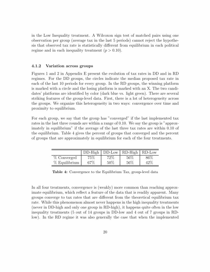
in the Low Inequality treatment. A Wilcoxon sign test of matched pairs using oneobservation per group (average tax in the last 5 periods) cannot reject the hypothe-sis that observed tax rate is statistically different from equilibrium in each politicalregime and in each inequality treatment (p > 0.10).

4.1.2 Variation across groups

Figures 1 and 2 in Appendix E present the evolution of tax rates in DD and in RDregimes. For the DD groups, the circles indicate the median proposed tax rate ineach of the last 10 periods for every group. In the RD groups, the winning platformis marked with a circle and the losing platform is marked with an X. The two candi-dates’ platforms are identified by color (dark blue vs. light green). There are severalstriking features of the group-level data. First, there is a lot of heterogeneity acrossthe groups. We organize this heterogeneity in two ways: convergence over time andproximity to equilibrium.

For each group, we say that the group has ”converged” if the last implemented taxrates in the last three rounds are within a range of 0.10. We say the group is ”approx-imately in equilibrium” if the average of the last three tax rates are within 0.10 ofthe equilibrium. Table 4 gives the percent of groups that converged and the percentof groups that are approximately in equilibrium for each of the four treatments.

DD-High DD-Low RD-High RD-Low

% Converged 75% 72% 56% 86%% Equilibrium 67% 50% 56% 42%

Table 4: Convergence to the Equilibrium Tax, group-level data

In all four treatments, convergence is (weakly) more common than reaching approx-imate equilibrium, which reflect a feature of the data that is readily apparent. Manygroups converge to tax rates that are different from the theoretical equilibrium taxrate. While this phenomenon almost never happens in the high inequality treatments(never in DD-high and only one group in RD-high), it happens quite often in the lowinequality treatments (5 out of 14 groups in DD-low and 4 out of 7 groups in RD-low). In the RD regime it was also generally the case that when the implemented

20

tax rates converged the candidate platforms also converged, although Group 2 inRD-low is an exception.

4.1.3 Voter Behavior

Besides making predictions about the equilibrium tax rate as a function of the distri-bution of productivities, the model also makes more specific predictions about voterbehavior in the two institutional regimes. Specifically, in DD, all voters, regardlessof productivity, have a dominant strategy to propose their most preferred tax rate,assuming all voters supply labor optimally conditional on any tax rate. Similarly,in RD, voters have a dominant strategy to vote for the candidate who proposed themore preferred of the two candidates’ tax rates, once again under the assumptionthat all voters supply labor optimally. In this section, we investigate voter behaviorrelative to these two benchmarks. In a later section, we compare it to an alternativebenchmark, where induced preferences over tax rates are inferred from the empiricallabor supply curves rather than the theoretically optimal labor supply curves.

Tax Proposals in DD

Figure 3 displays the mean and median tax proposal, by productivity, in the DD-High and DD-Low treatments, pooling across all groups for the last 10 periods, andcompares it with the theoretical peak of the induced voter preferences. In all casesthe observed mean or median proposals match up closely with the theory. In partic-ular, the average proposals by the median voter, with a productivity of 10 is almostexactly equal to the predicted proposal (0.54 vs. 0.53 in DD-low and 0.27 vs. 0.28in DD-high). There are a few small discrepancies that are worth noting. First, forhigh productivity voters who are predicted to propose zero tax, on average the pro-posal is for a tax rate of about 0.10. Second, in DD-high, the mean proposals arenot perfectly ordered by productivity. The second lowest productivity worker havea higher mean proposed tax rate than the lowest productivity voters (0.59 vs. 0.56),but this difference is not statistically significant. We also note that while the aver-age observed tax proposals match theoretically predicted ideal ones, there is a lot ofvariance in the proposals (as is evident from the relatively large standard errors).

Because of the within productivity variation in tax proposals, the observed medianproposal in a DD election will often come from a voter other than the voter withmedian productivity (10). Furthermore, the distribution of proposals across produc-tivities will induce a distribution of winning (i.e., median) proposals, with positive

21

Figure 3: Proposed Tax Rates, by productivity.

variance. Using the actual distributions used to construct Figure 3, one can simu-late many groups under the assumption that proposals are generated iid accordingto these empirical distributions, effectively bootstrapping our data to get tight esti-mates of the distribution of implemented tax rates.

Voting Behavior in RD

Table 5 summarizes voting behavior in each inequality treatment in the RD regimebroken down by productivity level, pooling across all groups for the last 10 periods.The first column lists the fraction of correct votes: a vote is labeled correct if thecandidate the voter voted for offered a proposed tax rate that theoretically wouldyield at least as high a payoff as the proposed tax rate offered by the other candi-date (provided that labor market behavior exhibit no deviations from the predictedone by the theory). The second column indicates the number of the correct votesincluding the number of cases in which both candidates proposed the same tax ratein the parenthesis. The third and the fourth columns list the number of mistakesseparated into two categories: the mistakes in which participants voted for a higherof the two proposed taxes is in column three, and the mistakes in which the vote wascast for the lowest of the two proposed taxes is in column four. Table 5 suggests thatthe majority of votes casted in the RD treatment were ”correct” independent of theproductivity level of the participants, with more accurate voting behavior observedin the Low than in the High inequality treatment. Moreover, the distribution of

22

mistakes of the pivotal agent is quiet balanced. Put differently, agents with produc-tivity of 10 in both inequality treatment tend to make mistakes in both directions:sometimes vote for the higher tax rate when the lower one theoretically would benefithim and other times vote for the lower tax rate when the opposite is true.

High Inequality

Productivity % correct # correct (indiff) # voted higher # voted lower

2 0.71 50 (6) 15 56 0.61 43 (6) 20 710 0.71 50 (6) 13 714 0.73 51 (6) 14 535 0.89 62 (6) 8 0

Low Inequality

Productivity % correct # correct (indiff) # voted higher # voted lower

2 0.80 56 (13) 7 76 0.69 48 (13) 9 1310 0.67 47 (13) 11 1214 0.91 64 (13) 6 018 0.91 64 (13) 6 0

Table 5: Voting Behavior in RD regime

Figure 4 provides a more complete description of voting behavior in the RD sessions,again broken down by productivity level and High vs. Low inequality. Each panel inthe figure displays simultaneously the two proposals that are offered in each electionand the proposal the voter of that productivity voted for. The horizontal axis rep-resents the tax rate proposed by the candidate the voter voted for, and the verticalaxis corresponds to the tax rate proposed by the other candidate. Each panel alsohas two crossing line segments. Those line segments represent pairs of tax proposalsthat the voter in theoretically indifferent between. One of the segments, the upwardsloping one, obviously is the diagonal. The other, downward sloping line representpairs that are equidistant from the voter’s ideal tax rate. The two lines intersect atthe ideal tax rate of the voter. Therefore, correct votes are votes that are in the twoquadrants that are north and south of the ideal point. Incorrect votes are in the eastand west quadrants.15 An interesting observation from these graphs is that incorrect

15For high productivity voters whose ideal point is zero tax, the west and south quadrants do not

23

votes in the Low inequality treatment tend to be votes for the higher tax rate whenit is inferior (west quadrant), but incorrect votes in the High inequality treatmenttend to be votes for the lower tax rate when it is inferior (east quadrant). Note alsothat most of the incorrect votes lie fairly close to one of the two indifference-pair linesegments.

4.2 Economy: Labor Market Behavior

Table 7 reports the mean difference between actual labor choices of agents and thepredicted one, broken down by the productivity levels and treatments. Our datashows that overall aggregate behavior of agents in the labor market is close to theone predicted by theory. However, in general agents with low productivity some-what oversupply labor, while agents with high productivity somewhat undersupplyit. This undersupply of labor is especially pronounced for agents with the highestproductivity of 35 in the High Inequality treatments in both regimes: these agents onaverage choose labor about 3 units away from the theoretically predicted one. Thisis an interesting behavioral finding, as both the undersupply by high wage workersand the oversupply by low wage workers contradict some currently popular models ofinequality aversion (see Appendix C for the characterization of optimal labor supplyof agents that have altruistic or Fehr-Schmidt preferences). We will investigate laterthe group-level data to see whether this result is driven by some specific individualsor it is a general trend.

A more rigorous statistical analysis of the labor supply behavior leads to a similarconclusion. Rewriting equation (2), we define the normalized labor supply function,L(t), as:

L(t) ≡ x∗i (wi, t)

wi

= 1− n− 1

nt

Table 8 reports the estimates obtained by regressing observed normalized labor sup-ply ( xi

wi) on a constant and the tax rate. We do this separately for each productivity

level. Because we have a total of 40 groups in all and 20 observations per group,this gives us 800 observations for each of the four lower productivity levels (whichare the same in both the high and low treatments), and 400 observations for thehigh productivity voters (which are different in the high and low treatments). Forthe highest productivity worker in the High inequality treatment (wi = 35), the con-straint xo ≤ 25 is binding if the tax rate is sufficiently low (t ≤ 0.375). So we run

exist, reflecting the fact that it is always optimal for these voters to vote for the lower tax rate.

24

Figure 4: Voting Behavior in RD regime.

25

High Inequality treatmentDD regime RD regime

first 10 last 10 first 10 last 10

Productivity 2 0.86 0.41 0.41 0.003Productivity 6 0.97 0.12 1.17 -0.29Productivity 10 0.69 0.30 -0.67 -0.56Productivity 14 0.82 0.25 -0.12 -0.20Productivity 35 -2.40 -3.20 -2.60 -2.86

Low Inequality treatmentDD regime RD regime

first 10 last 10 first 10 last 10

Productivity 2 0.87 0.45 0.76 0.17Productivity 6 0.69 0.11 0.41 -0.24Productivity 10 0.20 0.38 0.20 0.13Productivity 14 -0.06 -0.01 -0.82 -0.21Productivity 18 -0.46 -0.46 0.003 0.05

Table 6: Mean Difference Between Actual Labor Choice and Predicted One

separate regressions for t ≤ 0.375 and t > 0.375 for this one class of worker-voters.Thus, the table reports the estimates of the constant term α and the coefficient onthe tax rate, β for a total of seven different regressions.16 According to the theoreti-cal normalized labor supply equation, the estimates for the first six (unconstrained)regressions are predicted to be α = 1.0 and β = −n−1

n= −0.8. For the constrained

Tobit regression, the predicted estimates are α = 0.71 and β = 0.0.

The results reported in Table 8 are largely consistent with the theory, the two excep-tions being the slope of the response to the tax rate for the very lowest productivityworker and the very highest productivity worker when the constraint xo ≤ 25 isbinding (last row). In the former case, labor supply is under-responsive to the taxrate, and in the latter case it is over-responsive. Despite the closeness of the esti-mated parameters to the theoretical prediction, there is still a considerable amountof residual variance. The average adjusted R2 across the regression was XX.

16In all regressions, we report the statistics from a Tobit regression where labor choice is con-strained to be between 0 and 25.

26

Productivity α p-value β p-value

2 1.17(0.15) 0.26 −0.46(0.19) 0.076 1.04(0.05) 0.38 −0.74(0.08) 0.4310 1.01(0.02) 0.46 −0.74(0.05) 0.2114 1.02(0.02) 0.47 −0.79(0.03) 0.8818 0.97(0.03) 0.30 −0.76(0.05) 0.4635 (t > 0.36) 0.98(0.08) 0.77 −0.84(0.10) 0.7235 (t < 0.36) 0.65(0.04) 0.11 −0.73(0.09) 0.02

Table 7: Estimates of the Regression Analysis of the Labor Supply Functions of Agents.

Our preliminary analysis of the labor supply functions of subjects participated in theexperiment show no significant deviations from the ones predicted by the standardutility function specified in equation (1). In particular, this means that we do notobserve behavior consistent with either Fehr-Schmidt or altruistic preferences. Putdifferently, our experimental data reveal that in the redistributive environment, inwhich subjects’ actions affect not only their own payoffs but directly affect payoffsof other subjects through the taxation scheme, we do not detect preferences forredistribution beyond what the standard utility maximization yields.

4.3 Welfare

There are two dimensions to consider in the welfare analysis of redistributive taxa-tion: equity (or related notions of redistributive justice) and efficiency.17 There is atradeoff between these two dimensions, and both are jointly determined by the taxrate determined in the political sector and the labor supply decisions made in theeconomic sector. Thus, the welfare analysis must consider the combined politicaleconomy effects in the two sectors. The tradeoff is explicitly modeled in the the-oretical framework we use: the more pre-tax income is going to be redistributed,the less labor will be supplied. Assuming that each worker chooses his labor supplyoptimally given the tax rate (i.e., according to equation xxx), we can construct anequity-efficiency frontier, for any particular measure of equity and efficiency. Here wesimply use the post-tax gini coefficient as our measure of inequality, and total incomeas the measure of efficiency.18 Using these measures, we define the equity-efficiency

17cites to welfare economics literature or social choice literature18There are alternative measures as well, such as the variance of the income distribution to

measure inequality or netting out the effort costs of labor in the measure of efficiency.

27

frontier as the locus of points in this two dimensional space corresponding to aftertax equity-efficiency pairs that would arise from optimal labor supply behavior aswe vary tax rates from 0 to 1. We use this as a benchmark with which to come theactual equity-efficiency tradeoff that is observed in the experiment. Figure 7 displaysall the equity efficiency pairs for all group outcomes in the low inequality and highinequality treatments, respectively. The solid line in the figures marks the frontier,with the upper left of the frontier lines corresponding to t = 1 and the lower right ofthese lines corresponding to t = 0.19

Figure 5: Efficiency-Equity Tradeoff.

One way to interpret the data in these figures is to think of points below the frontieras corresponding to groups where aggregate labor is undersupplied at the given taxrate, and points above the curve correspond to oversupply of labor. The predictedoutcome in equilibrium are () in the low inequality treatment and () in the highinequality treatment, corresponding to the equilibrium tax rates of xx and yy, re-spectively. For the low inequality groups, deviations from the frontier are minimaland the direction of those deviations are balanced between points above and belowthe frontier, and is not correlated with the tax rate.20 For the high inequality groups,

19The frontier as we have defined it does not represent the boundary of feasible equity-efficiencypairs. In principle, workers are free to supply 25 units of labor for any tax rate, but doing so is notconsistent with equilibrium in our labor market.

20The deviations are slightly higher in the DD treatment than the RD treatment, but are stillsmall in magnitude.

28

High Inequality treatmentt = 0 t∗ = 0.53 t = 1 mean DD mean RD

Gini coefficient 0.628 0.313 0.000 0.326 0.296Total group GNP 1211 899.14 312.20 822.47 811.22

Low Inequality treatmentt = 0 t∗ = 0.28 t = 1 mean DD mean RD

Gini coefficient 0.485 0.349 0.000 0.380 0.354Total group GNP 660 512.16 132 543.45 517.17

Table 8: Equity-Efficiency Tradeoff.

the picture that emerges is much different. There is is much greater deviation fromthe frontier, and it is both unbalanced and correlated with the tax rate. There aremuch greater deviations below the frontier than above it, and these deviations aregreatest when the tax rate is relatively high. The main source of these large devia-tions is due to the undersupply of labor by the highest productivity types (w = 35),which is consistent with the labor supply decisions summarized in Table 8. Table 9below gives the averages across all the equity-efficiency pairs for the two treatments,with standard errors in parentheses (clustered by group).21

4.4 Empirical Equilibrium

The results so far paint a picture of the data as being close to the theory if one fo-cuses on the qualitative comparative statics and quantitatively at the average labormarket behavior and tax rates. However there is considerable variance in the data,as illustrated in the group-by-group tax rates series in figures xx and yy, and thedistribution of DD tax proposals in figure zz. In this section, we look Equilibriumtax rates crucially depend on expectations about the labor supply responses to taxes.We explore this variation across groups more carefully in this section.

Theoretically, deviations from equilibrium labor supply decisions in the economicsector could lead to distortions in the political equilibrium tax rates. That is, theequilibrium tax rates in High and Low Inequality treatments derived in Section 2only constitute an equilibrium if all agents make optimal labor decisions at all tax

21test for significant difference from equilibrium prediction

29

rates. However, to the extent that we find actual labor supply functions to be dif-ferent from the theoretical ones, and these deviations are different across groups,then one should expect rational candidates to propose different tax rates in the RDregime and agent to offer different tax proposals in the DD regime. Therefore, inthis section we will connect the analysis of the labor and political markets and askwhether the distortions in the labor supply in different groups is linked in this wayto the variation in tax rates that we observed.

To do this, we construct several models of ”empirical equilibrium” (EE) tax rates.That is, we estimate individual empirical labor supply functions of each agent in eachgroup, and then compute the equilibrium tax in each group for the estimated laborsupply functions of the five worker-voters in the group. The challenging part is ob-taining good estimates of the labor supply functions. We propose three different EEmodels. The first, EE1, uses only the data from the first 10 periods to estimate thelabor supply functions of each group member, and uses this to compute the medianvoter’s ideal tax rate as the basis for the empirical equilibrium tax rate. The second,EE2, is similar, but uses the labor supply data from all 20 periods. The third model,EE3, is a bit different. For each group EE3 is based on the earnings of the medianproductivity worker across the ten trial tax rates in the first 10 periods; the EE3 taxrate is the one of these for which that agent had the highest earnings.

Figure 8 displays a scatter graph of the three EE model tax rates on the verticalaxis against the observed tax rates on the horizontal axis, for each group.22 Theleft panel in each figure is for the High inequality treatment and the right panel isfor the Low inequality treatment, aggregating across both political institutions. Thetheoretical equilibrium assuming optimal labor supply is also shown on the graph,which is just a horizontal line at 0.53 for the High treatment and 0.28 for the Lowtreatment). Table 10 shows the results of regressing predicted against observed taxrates, using all 400 observations from the 40 groups in the experiment.

The theoretical model nails the coefficients almost exactly. A perfect theory wouldhave an intercept equal to 0 and a slope equal to 1. The theoretical equilibriummodel has an intercept equal to 0.00 and a slope equal to 0.94, and we cannot rejectthe hypothesis that they equal 0 and 1, respectively. All three EE models reject thathypothesis. In fact, for EE1 and EE2, one cannot even reject the hypothesis that the

22The ”observed” tax rate in each group equals the median of that group’s ten implemented taxesin periods 11-20.

30

0.0  

0.2  

0.4  

0.6  

0.8  

1.0  

0.0   0.2   0.4   0.6   0.8   1.0  

Theory  

EE1  

EE3  

EE4  

observed  median  tax  (last  10  rounds)  

High  Inequality  treatment  

0.0  

0.2  

0.4  

0.6  

0.8  

1.0  

0.0   0.2   0.4   0.6   0.8   1.0  

Theory  EE1  EE2  EE3  

observed  median  tax  (last  10  rounds)  

Low  Inequality  treatment  

Figure 6: Empirical Equilibrium Models

constant slope R2

Theory -0.00 (0.07) 0.94 (0.17) 0.28EE1 0.23∗ (0.06) 0.12∗∗ (0.13) 0.31EE2 0.23∗ (0.07) 0.11∗∗ (0.13) 0.31EE3 0.12∗ (0.06) 0.32∗∗ (0.14) 0.35

Table 9: Regressions of predicted against observed tax rates.∗ = significantly different from 0∗∗ = significantly different from 1

31

slope equals 0. On the other hand, the R2 is slightly higher for the three EE modelsthan the theoretical equilibrium model, but this does not take into account that weare implicitly burning some degrees of freedom by estimating the labor supply curvesfor each group and then feeding those estimates into each of these models.

5 Conclusion

The main conclusions are as follows: (1) There is a significant and large comparativestatic effect: higher inequality leads to more income redistribution (higher taxes)whether taxes are determined by direct democracy or representative democracy; (2)Both regimes implement the ideal tax rates of the median productivity agents. Thatis, for both regimes and both the High and Low treatments, average tax rates werenot significantly different from the theoretical tax rate. (3) Labor supply decisionsby agents are approximately optimal, with the exception that it is systematicallyundersupplied by high income agents. (4) There was considerable variation in im-plemented tax rates across groups, and in a number of cases variation over the 10periods within a group. (5) The variation of tax rates across groups does not appearto be linked with the variation of empirical labor supply functions across groups.

References

[1] Andreoni, J. and J. Miller (2002) Giving According to GARP: An ExperimentalTest of the Consistency of Preferences for Altruism. Econometrica. 70(2): 737-753.

[2] Carbonell-Nicolau, O. and E. Ok (2007). Voting over Income Taxation. Journalof Economic Theory 134: 249-86.

[3] Coughlin, P. (1992) Probabilistic Voting Theory. Cambridge University Press:Cambridge.

[4] Durante, R. and L. Putterman (2009). Preferences for Redistribution and Per-ception of Fairness: An Experimental Study. Working Paper, Brown University.

[5] Fisman, R., S. Kariv, and D. Markovits (2007). Individual Preferences for Giv-ing. American Economic Review. 97(5): 1858-76.

[6] Hinich, M. (1977) Equlibrium in Spatial Voting: The Median Voter Result is anArtifact. Journal of Economic Theory. 16: 208-19.

32

[7] Hochtl, W., J.-R. Tyran, and R. Sausgrubeer (2012). Inequality Aversion andVoting on Redistribution, European Economic Review, in press.

[8] Konrad, K. and F. Morath (2011). Social Mobility and Redistributive Taxation.Working paper #2011-2, Max Planck Institute for Tax Law and Public Finance,Munich.

[9] Krawczyk, M. (2010). A Glimpse Through the Veil of Ignorance: Equality of Op-portunity and Support for Redistribution. Journal of Public Economics, 94:131-41.

[10] Ledyard, J. (1984) “The Pure Theory of Large Two-Candidate Elections,” Pub-lic Choice, 1984, 44(1), 7-41.

[11] Meltzer, A. H., and Richard, S. F. (1981). A rational theory of the size ofgovernment. Journal of Political Economy 89 (Oct.): 914-927.

[12] Meltzer, A. H., and Richard, S. F. (1983). Tests of a rational theory of the sizeof government. Public Choice, 41, 403–418.

[13] Milanovic, B. (2000) The median-voter hypothesis, income inequality, and in-come redistribution: an empirical test with the required data. European Journalof Political Economy

[14] Perotti, R., 1996. Growth, income distribution, and democracy: what the datasay. Journal of Economic Growth 1, 149–187.

[15] Roberts, K. W. S. (1977). Voting over income tax schedules. Journal of PublicEconomics 8:329-340.

[16] Romer, T. (1975). Individual welfare, majority voting and the properties of alinear income tax. Journal of Public Economics, 4, 163–185.

[17] Tyran, J.-R. and R. Sausgruber. (2006) A Little Fairness may Induce a Lot ofRedistribution in Democracy, European Economic Review 50(2): 469-85.

33