equilibrium without independence*econweb.ucsd.edu/~vcrawfor/crawjet90.pdf · equllibrlum without...

IOUKNAL OF ECONOMIC THEORY 50, 1277154 (1990)

Equilibrium without Independence*

VINCENT P. CRAWFORD

Received May 23, 1988; revised February 14, 1989

Because players whose preferences violate the von Neumann-Morgenstern independence axiom may be unwilling to randomize as mixed-strategy Nash equilibrium would require, a Nash equilibrium may not exist without independence. This paper generalizes Nash’s definition of equilibrium, retaining its rational- expectations spirit but relaxing its requirement that a player must bear as much uncertainty about his own strategy choice as other players do. The resulting notion, “equilibrium in beliefs,” is equivalent to Nash equilibrium when independence is satistied, but exists without independence. This makes it possible to study the robustness of equilibrium comparative statics results to violations of independence. Jotuna/ of’ Gononric, Lirerarurr Classification Numbers: 022, 026. ” 1990 Academic

Press. inc.

1. INTRODUCTION

The expected utility analysis of decision-making under uncertainty rests on four assumptions about individuals’ preferences over lotteries, now commonly called completeness, transitivity, continuity, and independence. Completeness, transitivity, and continuity ensure that an individual chooses among lotteries as if to maximize a continuous preference function whose arguments are the probabilities of the possible outcomes. This follows from Debreu’s [16] representation theorem in consumer theory, because the probabilities are formally analogous to the (deterministic) quantities of goods over which consumers’ preferences are defined. Inde- pendence requires, for any positive probability p and lotteries A, B, and C, that A be weakly preferred to B if and only if a p: (1 -p) chance of A or C is weakly preferred to a p: (1 -p) chance of B or C. This goes far beyond

* This paper is an extensively revised version of Crawford [ 111, which combines the material in Crawford [ 12, 131. I am grateful to Robert Aumann, Cohn Camerer. Eddie Dekel. Yong-Gwan Kim, David Kreps, James Mirrlees, William Neilson, Robert Rosenthal, Dennis Smallwood, Maxwell Stinchcombe, and, especially, Mark Machina for helpful criticisms and suggestions. The National Science Foundation provided financial support under grants SES 8204038, SES 8408059. and SES 8703337.

642 51, 1-s

127 OO22-0531/90 $3.00

CopyrIght c IYYO by Academac Press. Inc All rights ol reproductmn ,n any fur,,, rexwed

128 VINCENT P. CRAWFORD

the analogy with consumer theory, implying, in conjunction with the other axioms, that the preference function is linear in the probabilities, so that it can be represented as the mathematical expectation of a von Neumann Morgenstern utility function.

The normative appeal and descriptive usefulness of the expected utility hypothesis have been the subject of controversy ever since the work of von Neumann and Morgenstern [38] brought it to the forefront of research in decision analysis and the theory of games. Independence has been more often criticized than the other three axioms, due in part to several commonly observed systematic experimental violations of the linearity it implies and perhaps in part to the persuasive power of the analogy with consumer theory. ’

Stimulated by this criticism, Machina [27, 281 showed that replacing the linearity in the probabilities implied by independence with the local linearity of a differentiable preference function yields a “generalized expected utility analysis” that allows a convincing and parsimonious explanation of the best-known experimental violations of the expected utility hypothesis, while preserving many of the techniques and results of expected utility analysis. The standard expected utility characterizations of risk aversion and increasing risk, and of monotonicity and first-order stochastic dominance, in particular, can be extended to give useful characterizations that do not rely on independence. Generalized expected utility analysis thus shows that much of our understanding of individual decisions under uncertainty survives relaxation of the -systematically violated linearity assumption embodied in independence.

However, the influence of independence is even more pervasive in game theory than in decision analysis, and individuals whose nonstrategic decisions violate independence are unlikely to satisfy it in their interactive decisions. Knowing how much of our understanding of strategic behavior remains valid without independence might alter our view of important applications. It would be of great interest, in particular, to know whether the theory of auctions, the theory of bargaining, and the linear-program- ming approach to designing incentive schemes (as espoused by Myerson [34], among others) are robust to violations of independence.

Contemplating violations of independence raises basic questions-in game theory. The desire for a common, unifying principle of rationality in games and decisions (eloquently expressed by Aumann [ 11) makes one hope that independence, which is not needed to formulate a sensible notion of

’ The papers by Malinvaud 1331 and Samuelson [42] and the adjoining papers by Weld, Shackle, Savage, Manx, and Charnes in the October, 1952, issue of Ecunome~ricu provide interesting evidence on how independence was viewed before expected utility analysis became a standard tool.

EQUlLIBRlUM WITHOUT INDEPENDENCE 129

rational individual decisions under uncertainty, can be dispensed with in game theory as well. But without independence, mixed-strategy equilibrium as defined by Nash [35] may fail to exist in nonpathological games: Non-expected utility maximizing players whose preferences cannot be represented by functions that are everywhere quasiconcave in the probabilities’ may be unwilling to randomize as equilibrium would require, and the experimental evidence now available indicates that this strong quasiconcavity assumption is unlikely to hold in most applications.

What does rationality mean, if anything, in games whose players’ preferences violate independence? And to what extent does assuming independence when it is not warranted distort predictions of strategic behavior’? This paper begins to construct answers to these questions, focusing on finite matrix games with complete information. As indicated above, the quasiconcavity of players’ preferences plays a crucial role in the analysis. Section 2 introduces generalized expected utility analysis with simple thought experiments about individual decisions and uses them to develop intuition about quasiconcavity; it then discusses the experimental and theoretical work on quasiconcavity, finding scarcely more justification for assuming quasiconcavity than for assuming linearity. Section 3 extends Section 2’s decision analysis framework to games and formally describes the class of games to be studied.

Section 4 defines Nash equilibrium and shows that when not all players’ preferences are quasiconcave, a Nash equilibrium may fail to exist, even when mixed strategies are allowed. Section 5 defines “equilibrium in beliefs,” a notion of equilibrium that extends Nash’s, retaining its rational expectations spirit but relaxing its implicit requirement that a player must bear as much uncertainty about his own strategy choice as other players do.3 Equilibrium in beliefs is shown to be equivalent to Nash equilibrium whenever players have quasiconcave preferences, and therefore (given completeness, transitivity, and continuity) whenever independence is satisfied. Without quasiconcavity, however, the two notions differ, and a mixed- strategy equilibrium in beliefs exists whether or not players have quasiconcave preferences. (Mixed strategies are needed for this result only to the extent that players prefer them to pure strategies.) This existence result is a significant (though mathematically trivial) generalization of the Nash

’ From now on. a player whose preferences can be represented by a preference function that is quasiconcave (respectively. linear or quasiconvex) in the probabilities is said to have “quasiconcave preferences” (respectively. “linear preferences” or “quasiconvex preferences”).

‘See Aumann [l], Brandenburger and Dekel [S], and Harsanyi [23]. By relaxing this requirement, equilibrium in beliefs answers the comon “businessmen don’t randomize” objection to descriptive applications of mixed-strategy Nash equilibrium: If businessmen randomize in an equilibrium in beliefs, they do so only because they prefer to. given their beliefs.

130 VINCENT P.CRAWFORD

equilibrium existence results in the literature. By generalizing Nash’s notion of equilibrium, it extends the internal consistency of the idea of rationality that motivated Nash’s notion to a wide class of games in which violations of independence cause nonexistence of Nash equilbrium.

Section 6 records some observations about the relationship between Nash equilibrium and equilibrium in beliefs in games and linearized versions of the games. Section 7 studies how the comparative statics of equilibrium are altered by violations of independence, comparing the qualitative responses of equilibrium beliefs under alternative assumptions about the quasiconcavity, linearity, and quasiconvexity of players’ preferences. Quasiconvexity and linearity have similar (but not identical) implications for comparative statics, but quasiconcavity and linearity can have qualitatively different implications.

Section 8 concludes the paper by discussing related work.

2. QUASICONCAVITY AND INDIVIDUAL DECISIONS

This section uses simple thought experiments about individual decisions to introduce generalized expected utility analysis, and discusses some of the qualitative features of the stochastic choices among lotteries generated by strictly quasiconcave preferences. It then summarizes the experimental and theoretical work that is helpful in evaluating the quasiconcavity assumption:

In this section, I restrict attention to three-outcome lotteries with known probabilities. The three outcomes are quantities of money, denoted y,, y2, and .v3, with y, <y2 <J’~; their probabilities are denoted s,, s2, and s3. As noted above, an individual with complete, transitive, and continuous preferences over lotteries chooses as if to maximize a continuous preference function whose arguments are the probabilities of the possible outcomes. Following Machina [27], this function is assumed to be differentiable, and the individual is assumed to prefer first-order stochastically dominating shifts in the distribution of money outcomes. To avoid confusion about the source of the phenomena to be discussed in this section, the individual is also assumed to be strictly risk-averse; and I restrict attention for simplicity to preferences that are either (globally) quasiconcave or (globally) quasiconvex.

It is also assumed that the individual can commit himself to abide by the outcome of a randomized choice among lotteries, even when he is not indifferent among the alternatives. Such commitments could be enforced by an experimenter. Without them, the individual might choose the alternative that is most preferred ex post without regard to the outcome of his randomization, making his ex ante choice irrelevant to his ultimate decision

EQUILIBRIUM WITHOUT INDEPENDENCE 131

and therefore (if he anticipates that he will renege) useless in inferring his preferences.4 Assuming commitment in this context is often considered innocuous (see, however, Aumann and Maschler [2, pp. P61-P62]), because it requires an expected utility maximizer to randomize only when he is indifferent among the possible outcomes. But commitments that violate this indifference condition may be optimal for quasiconcave preferences.

Figure 1 depicts the set of possible lotteries over the money outcomes y,, ?:2, and y.i.5 In the figure, S is a “status quo” lottery, A is an “alternative” lottery, and I, I, and I, I, are two of an individual’s indifference curves. Independence would require these to be linear and parallel, but I, I, and Z,Z, represent strictly quasiconcave preferences.

I,I, and Z,Z, also exhibit first-order stochastic dominance preference- that is, a preference for moving probability from low-money outcomes to high-money outcomes. The transition from the lottery (s,, s2, s3) to (6 2 4 3 s;) is a first-order stochastically dominating shift if and only if s; 3 s3 and si + s; 2 sZ + s3. Thus, the natural generalization of the assumption that money is desirable to choice over uncertain outcomes requires

0 ' =2

FIG. 1. Stochastic choice with quasiconcave preferences.

4 Machina [32], however, questions such mechanical impositions of dynamic consistency for decisions not significantly separated in time. Adopting his point of view would make my commitment assumption unnecessary,

’ Figure 1 differs from Machina’s [27. Fig. 5; 30, Figs. I l-141 diagrams in that it represents lotteries in (sz, s,)-space, suppressing S, = 1 - .F: - .Y~, instead of in (sr, s,)-space; the translation is straightforward.


that the individual prefer S to any lottery that lies to the southwest of the two dashed lines through S, and that he prefers any lottery that lies to the northeast of the two dashed lines to S. The indifference curve III, must therefore pass between the two dashed lines as shown, and similar restrictions must be satisfied at any other point in the triangle of possible lotteries. This is all that first-order stochastic dominance preference requires, for linear or nonlinear indifference curves.

The natural behavioral definition of risk aversion-aversion to mean- preserving spreads (see Rothschild and Stiglitz [41])--is equivalent to a uniform slope restriction on the individual’s indifference curves. The only mean-preserving spreads possible in the three-outcome case are reductions in s2 coupled with compensating increases in s, and s3. A mean-preserving spread therefore appears in Fig. 1 as a move to the northwest along a line with slope - [yr -,I’,]/[ y3 -J,]. A risk-averter must be made worse off by such a move, and must therefore have indifference curves that are uniformly steeper. The numerical magnitudes of .vl, v2, and y3, which do not otherwise enter my arguments, can be taken to be such that this is true for the indifference curves shown in Fig. 1.

Now imagine that the individual is offered a choice between the status quo lottery S and the alternative lottery A. When commitment to randomized choice is possible, he can also obtain any desired probability combination of the two. In Fig. 1, his choice set is then the line segment connecting S to A; the linearity of this segment follows from the laws of probability, and therefore holds with or without independence.

The individual’s choice probabilities vary with the alternative lottery A as follows. Construct the supporting line to Z,Z, at S, labeled LL in Fig. 1, and the offer curve (defined as in consumer theory!) through S, labeled 00. The probability, 71, with which he chooses the alternative lottery over S is zero for all alternatives below the supporting line and one for all alternatives above the offer curve, and varies continuously from zero to one as the alternative is varied from the supporting line to the offer curve. Note that an alternative that first-order stochastically dominates S must be chosen with probability one, but that, with strict quasiconcavity instead of linearity, many alternatives that would be preferred to S if randomized choice were not possible are chosen with probability less than one.

The offer curve appears in these unfamiliar surroundings beeause the individual’s randomized choice among lotteries is formally analogous to a consumer’s deterministic choice among consumption bundles in a com- petitive market.6 An individual whose preferences are quasiconcave exhibits

6 Machina [30] discusses further implications of this analogy and how individuals with quasiconcave preferences choose among lotteries in more general situations. Dekel [18] discusses the related question of how quasiconcavity and risk aversion interact to determine an individual’s preference for diversification of asset portfolios.


precisely the same kind of preference for “variety” that a quasiconcave utility function represents in ordinary consumer theory. A preference for variety is consistent with a complete, transitive, and continuous ordering over lotteries, hence is not irrational in the sense in which the term is normally used. Further, even though it can lead to randomized choice, the above arguments make clear that it is not inconsistent with risk aversion.

The thought-experiment just considered has completely different results if the individual’s preferences are quasiconvex. When an individual who can randomize chooses among a finite number of lotteries, his feasible set is the convex hull of those lotteries. A maximum of a quasiconvex function can always be found among the vertices of such a feasible set, and a maximum of a strictly quasiconvex function can occur only at a vertex. Individuals with strictly quasiconvex preferences, risk-averse or not, thus always choose either S with probability one or A with probability one in the thought-experiment, and their choice probabilities are therefore either locally constant or (in special cases) discontinuous in A. Such individuals would even pay a fee to avoid randomizing over lotteries between which they are indifferent. This striking behavioral difference between quasiconcavity and quasiconvexity is the basis of some of the experiments discussed below.

I now turn to the experimental work on quasiconcavity. It is important to note that the large body of evidence on violations of independence sum- marized in Machina [27, 28, 301 does not help to discriminate between quasiconcavity and quasiconvexity. Machina showed that almost all of the violations discussed in the literature can be elegantly explained by assuming that individuals have nonlinear preference functions that satisfy two simple hypotheses. These hypotheses are satisfied, under reasonable assumptions, by quasiconcave or quasiconvex quadratic preference functions. Thus, most of the evidence against linearity so far accumulated has no immediate implications for quasiconcavity.

Becker, DeGroot, and Marschak [3] found evidence of randomized choice, which, as noted above, is generally inconsistent with quasiconvexity: their experimental design, however, made it possible to detect violations of linearity only if they were in the direction of quasiconcavity. Coombs and Huang [lo] overcame this masking problem by asking experimental subjects to give complete rankings of two lotteries and a third formed by randomizing between them. Of their observations, 45% were inconsistent with linearity; 59% of these were consistent with strict quasiconcavity and the other 41% were consistent with strict quasiconvexity. In more recent experiments, Camerer [6], Chew and Waller [S], and Conlisk [9] all found strong evidence against independence, with the violations distributed roughly equally between quasiconcavity and quasiconvexity.


Turning to the relevant theoretical work, Kreps and Porteus [26] (see also Machina [29]) presented an interesting argument that favors quasiconvexity over quasiconcavity. They showed that in situations of “temporal risk,” in which an individual chooses among lotteries knowing that he must make an auxiliary decision before the uncertainty is resolved, an expected utility maximizer will have “induced preferences” that are nonlinear and quasiconvex. Although such choices can be handled within the expected utility framework by modeling the auxiliary decision explicitly, this is often not the most convenient way to proceed. When the analyst decides to leave the auxiliary decision in the background, the individual will appear to have quasiconvex preferences. More generally, unmodeled auxiliary decisions make the individual’s induced preferences “more quasiconvex” than his underlying preferences, preserving quasiconvexity and possibly overcoming quasiconcavity.

A different kind of induced-preferences argument, mentioned by Green [21, Section V], notes that if an individual optimally randomizes his choices, his derived preferences over lotteries must be quasiconvex.

Green [21] also studies whether an individual with nonlinear preferences can be induced to “make book against himself,” in the sense of accepting a series of gambles that together yield a final wealth distribution that is first-order stochastically dominated by the distribution that would result from not accepting the gambles. When the individual’s preferences satisfy independence, his choices are dynamically consistent, and it is an immediate consequence of first-order stochastic dominance preference that he will find any such series of gambles unacceptable. Noting that quasiconvexity is sufficient and, in general, necessary for dynamic consistency, Green shows that when it fails, the resulting inconsistency can be exploited to lead the individual to make book against himself. He argues that this is a strong argument in favor of assuming quasiconvexity (see, however, Machina’s [32] carrat).

3. GAMES WITHOUT INDEPENDENCE

This section describes the class of games to be studied. In the formal analysis, attention is restricted to two-person games of complete information in which each player has a finite set of pure strategies and each combination of pure strategies yields each player a deterministic quantity of money. The results and arguments extend immediately to n-person games of complete information with more complex outcomes. Vector outcomes


and shared background uncertainty, in particular, can be accomodated simply by reinterpreting players’ preference functions7

As in Section 2, it is assumed that each player can commit himself to abide by the outcome of a randomized choice among pure strategies, even when he is not indifferent among the distributions of outcomes they induce. The ability to make such commitments is implicit in the assumption that the player can use mixed strategies. In what follows, “mixed strategy” refers in general to a randomized choice of pure strategy, but is not meant to exclude unrandomized choices.

If players were expected utility maximizers, the games studied here could be completely described by specifying two matrices, one for the Row player (henceforth called R) and one for the Column player (henceforth called C), made up of the von Neumann-Morgenstern utilities whose expectations they maximize. To admit players whose preferences do not have an expected utility representation, it is necessary to separate their preferences over probability distributions of outcomes and the mapping from pure-strategy combinations to outcomes. R’s pure strategies are indexed by i = 1, . . . . nz, and C’s are indexed by j= 1, . . . . H. The m x n matrices r f [r;,] and c z [c,~] give R’s and C’s money payoffs as functions of their pure strategies, with r,, and c,; denoting R’s and C’s payoffs, respectively, if R plays his ith pure strategy and C plays, his jth pure strategy. Given this monetary payoff function, a combination of mixed strategies induces a probability distribution of money outcomes for each player. V(p; y) is the preference function that represents R’s preferences over these probability distributions,

’ Background uncertainty generally affects the quasiconcavity of players’ preferences, but my results are either independent of this or conditional on it. Footnote 8 below describes a device, due to von Neumann and Morgenstern [38, pp. 182-1861, that provides an alternative way to handle background uncertainty. Complete information means that the structure of the game (except for the realization of any shared uncertainty) is common knowledge; Aumann [l] and Brandenburger and Dekel [S] discuss the role played by this assumption and give references to the literature.

Incomplete information could be handled formally by summarizing players’ private information in parameters of their preferences called “types,” and assuming that players choose type-contingent strategies before observing their types, as in Harsanyi [22] (who introduced the notion of types and showed that it could be used to model the kinds of private information normally considered); see also von Neumann and Morgenstern 138, Chap. 191. This, together with the assumption that it makes no difference to a rational player whether he knows his type when he chooses his type-contingent strategy, turns a game of incomplete information into an equivalent game of complete information. But without independence, a player generally has different type-contingent preferences over type-contingent strategies before and after he observes his type. A further complication is that, with continuously distributed types, the possibility of puritication along the lines described by Harsanyi [23] arises. This possibility interacts in complex ways with the effect of violations of independence on players’ type-contingent preferences. An adequate treatment of games of incomplete information therefore involves signilicant new difficulties. which are not considered here.


expressed in terms of the mixed-strategy probabilities p E (p, , . . . . p,) and q = (41, ..., q,?) with which R and C play their pure strategies, and W(p; q)

is the analogous preference function for C. When independence is satisfied, V( .) and W( .) are linear in the

probabilities of the possible money outcomes, and therefore bilinear (and jointly continuous) in p and q. V( ) and W( .) can then be completely described by specifying the coefficients of these probabilities; these coefficients are players’ von Neumann-Morgenstern utilities for the possible outcomes. I assume instead, following Machina [27], that V( .) and W( .) are everywhere once (and in Section 7, twice) continuously differentiable.

The quasiconcavity of players’ preferences plays a central role in the analysis. A function ,f( .) is quasiconcave if its upper contour sets are convex-that is, if for any points x’ and x” in the domain of f( .) such that ,f(x’) > k and f(x”) 3 k, then f( (x’ + d/)/2) > k as well. Strict quasiconcavity is defined, in the usual way, by requiring the last inequality in this definition to hold strictly when x’ and x” are distinct. A function g( .) is (strictl?)) quasiconue.~ if -g( ) is (strictly) quasiconcave. Thus, linear functions are both quasiconcave and quasiconvex, but neither strictly quasiconcave nor strictly quasiconvex.

“V( .; q) is quasiconcave” (respectively, “V( .; q) is quasiconvex”) is short for “V(p; q) is quasiconcave in p for all q” (respectively, “V(p; q) is quasiconvex in p for all 4”). “W(p; ) is quasiconcave” (respectively, “W(p; .) is quasiconvex”) is short for “W(p; q) is quasiconcave in q for all p” (respectively, “W(p; q) is quasiconvex in q for all p”). The “strict” versions of these statements are used analogously. Because the probabilities of the possible outcomes in the game are linear in p for any given q, and vice versa, V( .; q) and W(p; .) are quasiconcave (respectively, continuous) when-and, except in special cases, only when-R’s and C’s underlying preferences over probability distributions of outcomes are quasiconcave (respectively, continuous) in the outcomes’ probabilities.

The term “upper contour set” refers below to the subsets of a player’s own mixed strategies that are required to be convex by the quasiconcavity of his preferences. A typical upper contour set for R, for instance, is a set of R’s mixed strategies, p, that satisfy V(p; q) 3 2) for a given mixed strategy, q, for C and a given constant, v.

4. NASH EQUILIBRIUM

This section defines Nash equilibrium and shows that, when players’ preferences are not quasiconcave, it may fail to exist in nonpathological games even when mixed strategies are allowed. Let argmax,,,f(x) denote the set of solutions of max it X,f(x), and let Sk denote the unit simplex in


il?, the set of mixed strategies feasible for a player with k pure strategies. Nash’s [35] definition of equilibrium can be stated as follows:

DEFINITION I. A Nash equilibrium is a pair of mixed strategies, (p*, q*), such that

p* E wwaxpt .y, 0: q* 1 and q*Eargmax,.s,l Wp*:q). (1)

Under the assumption that players are expected utility maximizers, Nash [35 J proved (generalizing to non-zero-sum n-person games a result of von Neumann [37] for zero-sum two-person games) that any finite matrix game of complete information has a Nash equilibrium when mixed strategies are allowed. In other words, Nash showed that if players’ strategy spaces are compact and convex, and each player’s preferences over strategy combinations can be represented by a preference function that is jointly continuous in both players’ strategies and linear in his own strategy for any given value of the other player’s strategy-as implied by the expected utility hypothesis when players’ strategies are vectors of mixed-strategy probabilities-then there exists a pair of strategies that are best replies to each other, as required by (1).

It is well known (see for example Debreu [15]) that Nash’s linearity assumption can be weakened to allow quasiconcavity. (In fact, von Neumann’s [37] original result for zero-sum two-person games assumed only quasiconcavity.) Thus, Nash’s existence result goes through if players’ preferences are nonlinear but quasiconcave. If they are not quasiconcave, there may be no Nash equilibrium in pure or mixed strategies, even though players’ strategy spaces are compact and convex and their payoff functions are continuous.

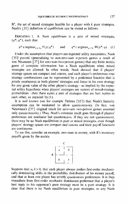
To see this, consider an example, zero-sum in money, with R’s monetary payoffs given by the matrix

C

R 0

R

El 0 h

Suppose that a, b > 0, that each player always prefers first-order stochasti- tally dominating shifts in the probability distribution of his money payoff, and that at least one player has strictly quasiconvex preferences. It is then immediate from first-order stochastic dominance preference that a player’s best reply to his opponent’s pure strategy must be a pure strategy. It is clear that there is no Nash equilibrium in pure strategies, so any Nash


equilibrium must involve each player playing both of his pure strategies with positive probability. But a player whose preferences are strictly quasiconvex is unwilling to randomize between distinct alternatives even when he is indifferent between them. His best replies to mixed strategies must therefore always be pure strategies when a # h, so there can be no Nash equilibrium in pure or mixed strategiesx

5. EQUILIBRIUM IN BELIEFS

Section 4’s example of nonexistence shows that Nash’s definition of equilibrium is not well suited to games whose players do not all have quasiconcave preferences. However, although our intuitions about rationality are inconsistent with a player’s probabilistic beliefs about other players’ strategies being systematically incorrect, even with complete information they do not require a player to bear as much uncertainty as other players about his own strategy choice. On the contrary, requiring an individual to bear uncertainty about his own decisions just because other players do is somewhat counterintuitive.

This section extends Nash’s definition of equilibrium by relaxing its equal-uncertainty requirement. The resulting notion of equilibrim, called “equilibrium in beliefs,” allows players with quasiconcave preferences (who may prefer the “variety” afforded by mixed strategies even when they yield

’ More formally, the set of probability distributions a player can bring about by varying his strategy for a given value of his opponent’s strategy is the convex hull of a finite number of points. A maximum of a strictly quasiconvex function over such a set must occur at a vertex; when the set is nondegenerate, which is always true in the example when a # h, this requires him to play a pure strategy.

It is tempting to conclude that there is no Nash equilibrium whenever there is no pure- strategy Nash equilibrium and players’ preferences are strictly quasiconvex. My argument does not quite show this, and considering the example with a = h makes clear that it is not true. When u = h, there is a strategy combination (in which each player plays each of his pure strategies with equal probability) such that neither player can unilaterally change the probability distribution of money outcomes. Such a combination must be in Nash equilibrium for any specification of players’ preferences in which they depend only on the probability distribution of money outcomes. The existence of this kind of equilibrium, in conjunction with the nonexistence just noted for all members of a wide class of neighboring games, is not incompatible with the upper hemi-continuity of the equilibrium correspondence, but it is somewhat startling. It is therefore natural to ask how common such equilibria are. This question was answered for finite zero-sum two-person games by von Neumann and Morgenstern 138. pp. 18221861 in the process of inventing a device for reducing background uncertainty to mixed-strategy uncertainty. They showed that in such games, there is an equilibrium at which neither player can unilaterally alter the probability distribution of money outcomes if and only if each payoff appears the same number of times in each row, and in each column, of the payoff matrix. This suggests that games in which a mixed-strategy Nash equilibrium exists despite players’ having strictly quasiconvex preferences are extremely rare.


no strategic benefits; see Section 2 or Machina [30]) to take full advantage of their randomization possibilities, while letting players whose preferences are not quasiconcave reap the strategic benefits of mixed strategies without enduring the associated uncertainty.

It is shown that equilibrium in beliefs is completely equivalent to Nash equilibrium whenever players have quasiconcave preferences, so that, although Nash’s equal-uncertainty requirement is arbitrary, it is also innocuous when independence is satisfied. But without quasiconcavity the two concepts differ, and a mixed-strategy equilibrium in beliefs exists whether or not players have quasiconcave preferences; mixed strategies are required for this result only to the extent that players whose preferences are not quasiconvex prefer them to pure strategies. Thus, equilibrium in beliefs provides an internally consistent formalization, without the assumption of independence, of the idea of rationality that motivated Nash’s definition of equilibrium, allowing a unified treatment of players with linear, quasiconcave, and quasiconvex preferences.

Equilibrium in beliefs can be defined as follows. For any set T of mixed strategies, let D[T] denote the set of probability distributions over the elements of T, each expressed as vector, conformable to a mixed strategy, that gives the ultimate distribution of pure strategies.

DEFINITION 2. An equilibrium irz helie@ is a pair of probability distributions, (P*, Q*), such that

p* E Warmax,..sna VP: Q*)l and Q*~~Cargmax,,,~ W(P*; q)]. (2)

P* and Q* should be thought of as C’s and R’s respective equilibrium beliefs about each other’s ultimate pure-strategy choices. (Lower case letters are used throughout for players’ mixed strategies, and upper case letters are used for players’ beliefs, when they may differ.) In the words of Aumann [l, p. 151:

. the players simply do not know what actions the other players will take. In “matching pennies”, each player knows very well what he himself will do, but ascribes i-i probabilities to the other’s actions, and knows that the other ascribes those probabilities to his own actions.

Equilibrium in beliefs requires each player’s beliefs about the other’s mixed strategy to be a (possibly degenerate) probability distribution over the other’s best replies, given his beliefs about the first player’s mixed strategy; the second player’s beliefs about the first player’s mixed strategy are required, in turn, to be the same as the first player’s beliefs about the second player’s beliefs, and so on. Once players’ beliefs are determined,


their best-reply correspondences are easily recovered. These correspondences completely summarize the implications of rational play in the game; players’ choices from them do not affect their (ex ante) equilibrium welfares, and are not determined by the model in any case.

Because equilibrium in beliefs explicitly allows for a player’s uncertainty about his opponent’s choice from his best-reply correspondence, it is reminiscent of Bernheim’s [4] and Pearce’s [39] notion of rationalizability. However, because its definition is formulated in terms of a single set of commonly held beliefs, it rests implicitly on the assumption that those beliefs are common knowledge (see Aumann [ 1 ] and Brandenburger and Dekel [IS, Section 4]), and is therefore more closely related to Nash equilibrium than to rationalizability. In fact, equihbrium in beliefs is equivalent to Nash equilibrium when players’ preferences are quasiconcave, hence when independence is satisfied; what I have called equilibrium in beliefs is therefore often viewed simply as an alternative interpretation of Nash equilibrium, with the equilibrating variables viewed not as players’ strategy choices, but as their beliefs. However, the distinction between Nash equilibrium and equilibrium in beliefs is substantive when not all players’ preferences are quasiconcave.

The equivalence of Nash equilibrium and equilibrium in beliefs when players’ preferences are quasiconcave follows from two observations:

OBSERVATION 1. [f‘ (P*, Q* ) is u Nash equilibrium in a game, it is ulso un equilibrium ill heli@ in that game.

ProoJ: Observation 1 follows immediately from Definitions 1 and 2, because an element of argmax,. s,, V( p; Q*) is also an element of DCargmax,.,m UP: Q*)l, and an element of argmax,. ,s, W(P*; q) is also an element of D[argmax,E,sfl W(P*; q)]. 1

OBSERVATION 2. If (P*, Q*) is an equilibrium in beliefs in a game in which players have quasiconcave prgferences, then (P*, Q*) is also a Nash equilibrium in that game.

Proox By Definition 2, an equilibrium in beliefs (P*, Q*) satisfies (2). Because argmax.,, r, f(x) is a convex set whenever f ( .) is quasiconcave and X is convex, the quasiconcavity of V(. ) and W( . ) then implies that (P*, Q*) satisfies (1 ), Definition l’s condition for a Nash equilibrium. 1

The equivalence of Nash equilibrium and equilibrium in beliefs is intuitively clear when players’ preferences satisfy independence. Then, a player’s uncertainty about his own equilibrium pure-strategy choice does not affect his welfare, because all choices to which his equilibrium mixed strategy assigns positive probability must be best replies, and independence

EQUILlBRlUM WITHOUT INDEPENDENCE 141

implies that he is indifferent about how uncertainty over indifferent outcomes is resolved. Strict quasiconcavity does not destroy this equivalence, because in equilibrium a player with strictly quasiconcave preferences always chooses to bear as much uncertainty about his pure-strategy choice as his opponent. (The game’s information structure does not allow him to bear more.)

The next result shows how Nash equilibrium and equilibrium in beliefs are related in games with players who do not have quasiconcave preferences, and are therefore unwilling to bear as much uncertainty about their own pure-strategy choices as their opponents do.

DEFINITION 3. The conuexgierd version of a game is obtained from the game by replacing each player’s preferences by the quasiconcave preferences whose upper contour sets are the convex hulls of his original upper contour sets (defined in Section 3), leaving other aspects of the game unchanged.

It can be shown, using Caratheodory’s Theorem, that players’ preferences in the convexified version of the game inherit the continuity of their original preferences.’

THEOREM 1. (P*, Q*) is an eqzrilibriunz in he1iqf.k in a game (f and onI) if it is a Nash equilibriun~ in the conoe.u$ied version oj‘ the game.

Proof: Suppose first that (P*, Q*) is an equilibrium in beliefs in a game. Because the “players” in the convexified version of the game have continuous, quasiconcave preferences, the proof of Observation 2 shows that (P*, Q*) satisfies (1) for the convexilied version of the game, and is therefore a Nash equilibrium in that game. Now suppose that (P*. Q*) is a Nash equilibrium in the convexilied version of a game. Then P* is in the convex hull of R’s (true) equilibrium upper contour set, and is thus a convex combination of his best replies to Q*. Similarly, Q* is a convex combination of C’s best replies to P*. Thus, (P*, Q*) satisfies (2), and is therefore an equilibrium in beliefs in the game. 1

Because the convexified version of a game whose players have quasiconcave preferences is the game itself, Theorem 1 subsumes Observation 2 and, when players have quasiconcave preferences, Observation 1 as well. Theorem 1 also makes it possible to deduce the existence of an equilibrium in beliefs from standard results:

‘See, for example, Rockafellar [40, Theorem 17.21. A different argument is required for games with more complex strategy spaces.


THEOREM 2. Any ,finite matrix game of’ complete information whose players have continuous preference functions has an equilibrium in beliefs.

Proqf Given Theorem 1 and the continuity of players’ convexilied preferences, the theorem follows immediately from Debreu’s [ 151 Social Equilibrium Existence Theorem, applied to the convexified version of the game. 1

Mixed strategies are needed for Theorem 2 only when players whose preferences are not quasiconvex prefer them to pure strategies, given their equilibrium beliefs. It is of course necessary to allow “mixed” beliefs in general, but this is not inconsistent with players playing pure strategies.

A straightforward extension of the arguments that underlie Theorems 1 and 2, working with the agent normal form (as in Karni and Safra [24,25]) or (as suggested by Machina 1321) ignoring the dynamic-consistency issues raised by violations of independence as irrelevant in games whose decisions are not significantly separated in time, yields the existence of a “subgame-perfected” version of equilibrium in beliefs under the assumptions maintained here. Theorem 1 suggests natural extensions of other refinements to equilibrium in beliefs; these are left for future work.

I conclude this section by using the example introduced in Section 4, with u> b >O, to illustrate the construction of an equilibrium in beliefs when players’ preferences are strictly quasiconvex. It follows from Section 4’s arguments that the convexified version of this example has no Nash equilibrium in which either player plays a pure strategy. Theorem 1 therefore implies that, given the strict quasiconvexity of players’ preferences, an equilibrium in beliefs (P:, P* ; QF, Q5) must satisfy

and

V(0, 1; Q:, Qr*)= Vl, 0; PI", Qz*)

W(PT, Pz*;O, I)= W(PF, PT; 1,O).

(3)

Continuity and first-order stochastic dominance preference ensure that (3) determines unique values of (PF, P:) and (Q:, QT), which are plainly in Nash equilibrium in the convexified version of the game and in equilibrium in beliefs in both the game itself and its convexilied version.

The construction of this equilibrium in beliefs is illustrated in Fig. 2. Probability distributions over the three possible outcomes, 0, a, and b, are depicted with the ex ante probability of R winning z from C denoted P(z), suppressing P(0) = 1 - P(a) - P(b). Figure 2 graphs each player’s equilibrium indifference curve, given the unique beliefs (P:, PT ; QT, QT) that satisfy (3). The intercepts of these indifference curves are located by noting that, because players’ ultimate pure-strategy choices are statistically


PIa)

Pl’

4’

0

FK. 2. Equilibrium in beliefs with quasiconvex preferences.

independent, P(a) = P, Q, and P(b) = P,Q,. Thus, when C’s beliefs about R’s ultimate pure-strategy choice are given by (Pf, PT), C can bring about any distribution on the line segment from (P(a), P(b)) = (P:, 0) to (P(a), P(b)) = (0, Pf) by varying his strategy from (Q,, Q2) = (1,O) to (Qt, Qd = (0, 1); (3) re uires q that he be indifferent between these two extreme points. Similarly, when R’s beliefs are given by (Q:, Q:), he can bring about any distribution on the line segment from (P(a), P(b)) = (Q:, 0) to (P(u), P(h)) = (0, Q;) by varying his strategy from (P, , Pz) = ( 1,0) to (P,, P2) = (0, 1); (3) again requires indifference between these points. It is easy to verify that these line segments intersect at (P: Q:, P? Q:), the equilibrium value of (P(a), P(h)). Given first-order stochastic dominance preference and that a > h > 0, R prefers higher values of P(a) and P(b), and C prefers lower values; R’s and C’s indifference curves are distinguished in each figure by arrows indicating these preference directions.

Figures 3 and 4 illustrate the construction of Nash equilibrium and equilibrium in beliefs when players’ preferences are respectively linear and quasiconcave. Figures 2 and 3 together illustrate Theorem 1. Figure 3 is constructed like Fig. 2. However, because Nash equilibrium and equilibrium in beliefs are no longer characterized by (3) when players have strictly quasiconcave preferences, Figure 4 is constructed by applying Observation 3 from Section 6 and then using the construction of Fig. 3.


P(1 I

4

Ql

I 3 I P(b)

FIG. 3. Equilibrium in beliefs (and Nash equilibrium) with linear preferences.

FIG. 4. Equilibrium in beliefs (and Nash equilibrium) with quasiconcave preferences

EQUILIBRIUM WITHOUTINDEPENDENCE 145

6. LINEARIZED GAMES

This section records two observations about Nash equilibrium and equilibrium in beliefs in games and linearized versions of the games.

DEFINITION 4. A player’s focal preference function at a given point is the linear preference function tangent to his preference function at that point. A player’s local preferences at a given point are the preferences represented by his local preference function at that point.”

A player’s local preferences satisfy independence by construction. When his preference function is differentiable, his local preferences at any given point are unique; the local preference function is then unique up to increasing transformations.

DEFINITION 5. The linearized version of a game at a given point is obtained from the game by replacing each player’s preferences by his local preferences at that point.

OBSERVATION 3. A Nash equilibrium in a game is also a Nash equi- Iibrium in the linearized uersion of the game at the equilibrium.

OBSERVATION 4. A Nash equilibrium in a game whose pla.yers have linear preferences is also a Nash equilibrium in any game whose players have quasiconcave preferences for which the game is the linearized version at the equilibrium.

Observations 3 and 4 are illustrated in Fig. 4. Their proofs follow immediately from the facts that a player’s preference function and his local preference function at a given point have the same first derivative at that point, and that the first-order conditions are sufficient as well as necessary for a maximum of a quasiconcave (or linear) function over a convex set. Mathematically, these observations are roughly analogous to the first and second basic theorems of welfare economics; note in particular that they rest on the same separation theorems, and that Observation 4, but not Observation 3, requires that players have quasiconcave preferences.

Together with Theorem 1, Observations 3 and 4 map out the relationship between Nash equilibrium and equilibrium in beliefs in games and their

” Here, linearity refers to the player’s underlying preferences over outcome probabilities; thus, his local preference function is bilinear in p and 9. Machina [27] worked instead with the “local utility function” that gives the coefficients of the outcome probabilities in the local preference function, just as the von Neumann-Morgenstern utility function gives those coetlicients for an individual with linear preferences. The local preference function contains the same information as the local utility function, and is more convenient for my purposes.


linearized versions. Theorem 1 shows that Observation 4 remains valid when “equilibrium in beliefs” replaces “Nash equilibrium” in its statement. This replacement invalidates Observation 3 unless players’ preferences are quasiconcave, because otherwise the linearized version of the convexitied version of a game generally differs from the convexitied version of the linearized version of the game. To see this, note that players’ indifference curves through the point (P(a), P(b)) = (P:Q:, PtQ$) in Fig. 2 need not be tangent to the dashed lines that represent the indifference curves of their convexitied preferences through that. point.

7. COMPARATIVE STATICS

This section considers how the comparative statics properties of equilibrium are altered by violations of independence. Attention is restricted, for simplicity, to games in which players’ preferences are either both strictly quasiconcave or both strictly quasiconvex.

Suppose first that players’ preferences are strictly quasiconcave, and recall that Nash equilibrium and equilibrium in beliefs are equivalent in this case. Observations 3 and 4 suggest the possibility of a useful correspondence between the qualitative comparative statics of equilibrium in a game and in its linearized version. This suggestion is reinforced by Machina’s [27, Theorem 41 (see also his discussion in [29, Section 21) demonstration that global restrictions on an individual’s local Arrow-Pratt measure of absolute risk aversion (that is, the Arrow-Pratt measure computed for the von Neumann-Morgenstern utility function associated with his local preference function) determine the qualitative comparative statics of his demand for safe versus risky assets in the same way with and without independence.

An optimistic conjecture about the correspondence might go as follows. (The term “game” is used loosely here, to refer to a specification of players’ strategy spaces and their monetary payoffs, leaving their preferences free to vary. )

Conjecrure. If a given qualitative comparative statics result holds in a game whenever its players have linear preferences in a given class, then it also holds for that game when players have nonlinear, differentiable preferences whose local preferences are everywhere in that class.

When players’ preferences are strictly quasiconcave, the conjecture is invalid for two reasons, one common to games and individual decisions, and one specific to games. The first reason is that the signs and magnitudes of comparative statics derivatives for individual decisions, and a.fortiori for games, depend in general on second-order as well as first-order partial


derivatives. Simple examples (see, for instance, Crawford [ 11, Section 61) show that the direction of an individual’s responses can change when his quasiconcave preferences are replaced by his local preferences. The second- order conditions determine the signs of the denominators of the comparative statics derivatives, and ensure that they are the same in each case; but the second-order restrictions implied by independence are generally instrumental in signing the numerators, which can therefore differ in sign between the two cases. Machina [27, Theorem 41 (see also Machina [31] and Neilson [ 361) avoids this diffkulty by placing stronger restrictions on individuals’ preferences-in this case, that the local absolute risk aversions of the individuals being compared are everywhere ordered in the same way-than are needed to establish the comparative statics results when their preferences satisfy independence. These restrictions make it possible to derive, from information about first-order partial derivatives, conclusions about behavior that would otherwise depend on second-order partial derivatives.

The second reason is that, in games as in individual decisions, the second-order conditions of individuals’ optimization problems are important in determining the signs of the denominators of comparative statics derivatives. But in games, the signs of these denominators (which are the determinants of matrices derived from the second-order partial derivatives of all players’ objective functions) are no longer completely determined by individuals’ second-order conditions. This leaves them free to differ between the game and its linearized version.

The example used in Sections 4 and 5 can be used to illustrate both of these sources of differences. Assume again that a> b>O, and treat the monetary payoff a as a parameter of V( .), assuming that C’s monetary payoff when each player plays his first pure strategy remains fixed at its initial value of -a. A totally mixed equilibrium in beliefs-that is, one in which each player’s beliefs assign positive probability to each of his opponent’s pure strategies-is characterized, substituting out P2 E 1 - P, and Q, = I - Q, for simplicity and interpreting the partial derivatives with these substitutions in mind, by the first- and second-order conditions

and

~V(P:,~-P:;Q:,~-Q:;~)/~P,=O,

~2v(f’T, l-P:;QT, l-QT;a)/dpf<O,

dw(p:, 1 -pi+; Q:, 1 -QF)/dQ, =o,

(4)

(5)

(6)

a2w(P:, 1 - PF; Q:, I- Q:)/~Q: ~0, (7)

where P: and P: denote the equilibrium values of P, and P2

148 VINCENT I’. CRAWFORD

Applying the Implicit Function Theorem to the system of first-order conditions composed of (4) and (6) yields

In (8), all functions are evaluated at the equilibrium values of P: and QT; and it is assumed that H, the determinant of the matrix on the left-hand side, is nonzero. (Note that even when players’ preference functions are linear, so that the diagonal elements of the matrix are zero, H is generically nonzero.) Applying Cramer’s Rule to (8) yields

and

dP:/da= -[a2V(.)/aP,aa][32W(.)/aQ:]/H (9)

dQf/da= -[a2V(.)/dP,aall[a2w(.)/aQ,ap,l/H. (10)

The conjecture fails for two reasons. First, when V( .) is linear, a’V( .)/aP, da must be positive if R prefers more money to less, but it is easily verified that this does not follow from first-order stochastic dominance preference when V(. ) is required only to be quasiconcave. The separability across outcomes implied by independence is instrumental in signing the numerators of the comparative statics derivatives in (9) and (10). Second, the determinant H is not signed by the second-order conditions of players’ optimization problems, and is therefore free to differ in sign from the analogous determinant in the corresponding game where V(. ) and W( -) are replaced by R’s and C’s local preference functions.

Now consider games whose players’ preferences are strictly quasiconvex, and recall that, by Theorem 1, an equilibrium in beliefs in such a game is equivalent to a Nash equilibrium in its convexilied version. Because players’ preferences in the convexified version of such a game are linear, this makes the conjecture highly plausible. Somewhat surprisingly, the analysis that follows shows that it is not quite correct.

It is assumed that the game has a totally mixed equilibrium inibeliefs. This is a significant restriction, required by the standard comparative statics methodology employed. However, in games that do not have a totally mixed equilibrium, the set of pure strategies that are “active” in equilibrium is almost everywhere unaffected by a small parameter change. Results derived for totally mixed equilibria therefore apply, locally, except for parameter values at which the set of active pure strategies changes, and thus hold locally for almost all games that do not have a totally mixed equilibrium. I consider only changes in the monetary payoff Y,, , abbreviated for clarity to r from now on; the results can be reinterpreted to obtain the effects of changing the other r,,, or the c,,.


Let e, denote a vector (of dimension determined by the context) with a one in the ith place and zeros everywhere else. It follows from Theorem 1 that the equilibrium in beliefs (P*. Q*) is characterized by the systems

V(e,;Q*;r)= -h,

V(ez; Q*; r) = -h,

(11)

V(e,; Q*; r) = -h,

iQ;= 1,

and

W(P*; e, ) = k,

W( P*; e2) = -k,

(12)

W( P*; e,) = -k,

tP:=l,

where h and k are constants to be determined. Systems (11) and (12) ensure that each player is indifferent, given his beliefs, between any two of his active pure strategies, and that the probabilities he assigns to his opponent’s playing his available pure strategies sum to one. System (12) reflects the fact that the parameter r, which appears as an argument of I’( .) in ( 1 l), does not directly affect C’s welfare.

Systems (11) and (12) closely resemble those that characterize a totally mixed Nash equilibrium when players are expected utility maximizers; compare systems (1) and (2) in Crawford and Smallwood [14]. Just as when independence is satisfied, a player’s beliefs about his opponent’s strategy make him indifferent between any two of his active pure strategies (although in this case he would not be indifferent between those pure strategies and randomizing over them), and the equations that determine one player’s equilibrium beliefs are completely separable from those that determine the others. Further, as standard equation-counting arguments show, for almost all games a totally mixed equilibrium can exist only when m = n, so that each player has the same number of active pure strategies.

To evaluate the conjecture in the quasiconvex case, note first that, just as when independence is satisfied, changing r has no effect on P* as long as the same sets of pure strategies remain active, because P* is determined

dv(e,; Q*; r)ldQ,

1 :

... dV(e,; Q*; r)/aQ, 1 dQ I”ldr dv(e,; p*; r)PQ, ... aV(e,,; e*; r)/i3Q,, ; dQ,*/dr I L 1 . . . 1 I : 0 dh/dr 1

-dV(e, ; Q*; r)/dr

0 L : 1. 0

(13)

0


by (12) alone. Further, r affects V( .) only when R plays his first pure strategy with positive probability, so that dV(e,; Q*; r)/& = 0 for all if 1. To compute the effect of changing r on Q*, apply the Implicit Function Theorem to (11) to obtain

(13) is derived under the assumption that the matrix that appears on its left-hand side has a nonzero determinant. The nonsingularity of this matrix for generic games reflects the fact that, even though C’s best reply is discontinuous in P at equilibrium when his preferences are quasiconvex, the value of Q* at an equilibrium in beliefs normally varies smoothly with r. This stands in interesting contrast to the discontinuity of individual decisions with quasiconvex preferences (see Section 2 or Machina [30]).

(13) can be solved by Cramer’s Rule to obtain the desired comparative statics derivatives, which are determined entirely by the first-order partial derivatives of V( .). Despite the fact that changing r generally affects these partial derivatives in complex ways when R’s preference function is nonlinear, (13) takes precisely the same form as when independence is satisfied: The same zero restrictions are satisfied, and the partial derivative d V(e,; Q*; r)/c3Qj is the nonlinear analog of R’s von Neumann-Morgenstern utility for the monetary payoffr,.

If the local von Neumann-Morgenstern utilities that make up the matrix on the left-hand side of (13) were evaluated at the same probability distribution of outcomes, the conjecture would therefore follow immediately from (13). Because they are not, the conjecture requires an additional assumption: When players’ preferences satisfy betweenness in the sense of Chew [7] and Dekel [17)-that is, when their preferences are both quasiconcave and quasiconvex, so that their indifference surfaces are linear (but not necessarily parallel)-local utilities evaluated at different distributions on the same indifference surface can be taken to be independent of where they are evaluated. This is precisely what is needed for the conjecture to hold.


When betweenness is replaced by strict quasiconvexity, the conjecture is invalid as stated. It fails, despite Theorem 1, because a player whose preferences are strictly quasiconvex has widely separated best replies. Thus, other players’ beliefs about his strategies are determined by global com- parisons, and local linearity of his preference function is not enough to justify a generalized expected utility analysis of his strategic responses. Betweenness overcomes this difficulty by extending local linearity to global linearity along the equilibrium indifference surfaces.

In general, if a qualitative comparative statics result holds in a game whenever its players have linear preferences in a given class, then it also holds for that game whenever players have quasiconvex, differentiable preferences such that local preference functions made up of their partial derivatives (possibly evaluated at different points) always fall in that class. This is considerably weaker than the conjecture. It shows, however, that the comparative statics of games whose players have quasiconvex preferences bear at least a family resemblance to the comparative statics of the corresponding games whose players are expected utility maximizers.

8. CDNCLUSION

This section concludes the paper by discussing related work. The earliest mention of the issues considered here of which I am aware

is a passage in von Neumann and Morgenstern [38, p. 1561 (paraphrased where indicated to remove dependence on context):

That the [payoff function] is a bilinear form is due to our use of the “mathematical expectation” whenever probabilities intervene. It seems significant that the linearity of this concept is connected with the existence of a solution. in the sense in which we found one. Mathematically this opens up a rather interesting perspective: One might investigate which other concepts, in place of “mathematical expectation,” would not interfere with our solution.-i.e. with the [minimax theorem] for zero- sum two-person games.

Interestingly, despite the apparently conclusive evidence in this quotation, there is ample evidence elsewhere in Theory of Games and Economic Behavior that relaxing independence is not what von Neumann and Morgenstern had in mind. They thought it desirable [38, pp. 6088616 and 63&632] to relax their assumptions that preferences are complete and continuous, and that they depend only on the ultimate probability distribution of outcomes (without regard to how that distribution was obtained by reducing compound lotteries). Of independence, however, they say only that it “expresses a property of monoton[icit]y which it would be hard to abandon” ([38, p. 6301; letters added for clarity). Aside from the experimental evidence accumulated in the last four decades, relaxing inde-


pendence may appear more interesting today than it did to von Neumann and Morgenstern because their original formulation made independence hard to separate from the rest of their axiom system (see Malinvaud [33] and Samuelson [42]).

Since von Neumann and Morgenstern wrote, there has been very little work in game theory outside the expected utility framework. Shapley and Shubik [44] outlined a generalization of the von Neumann-Morgenstern solution for n-person cooperative games that does not require independence. Weber [45] and Karni and Safra [24,25] found it useful to consider certain kinds of violations of independence in explaining behavior in auctions. Fishburn [ 191 established the existence of Nash equilibrium with a relaxed continuity assumption. And Fishburn and Rosenthal [20] (see also Shafer and Sonnenschein [43]) proved the existence of equilibrium when players’ preferences violate transitivity and independence in certain ways.

In recent years, non-expected utility decision models have given us significantly better explanations of observed behavior in nonstrategic environments. These successes, and the weight of the experimental evidence against the expected utility hypothesis, suggest that much might be learned about strategic behavior by basing applications of game theory on more general models of individual decisions under uncertainty. This paper has shown that at least one obstacle to such applications can be overcome.

REFERENCES

1. R. AUMANN. Correlated equilibrium as an expression of Bayesian rationality, Econometrica 55 (1987), l-18.

2. R. AUMANN AND M. MASCHLER. Some thoughts on the minimax principle. Manuge. Sci. 18 (1972), P54-P63.

3. G. M. BECKER, M. DEGROOT, AND J. MARSCHAK, An experimental study of some stochastic models for wagers. Eehau. 5%. 8 (1963), 199-202.

4. B. D. BEKNHEIM, Rationalizable strategic behavior, Economelrica 52 (1984) 1007-1028. 5. A. BRANDENBURCER AND E. DEKEL, Rationalizability and correlated eqyilibria,

Econometrica 55 (1987), 1391-1402. 6. C. CAMERER. An experimental test of several generalized utility theories, J. Risk Uncer-

tainty 2 (1989), 61-104. 7. S. H. CHEW, A generalization of the quasi-linear mean with applications to the measure-

ment of income inequality and decision theory resolving the Allais paradox, Econometrica 57 (1983), 1065-1092.

8. S. H. CHEW AND W. S. WALLER. Empirical tests of weighted utility theory, J. Math. Psych. 30 (1986), 55-72.

9. J. CONLISK, Verifying the betweenness axiom with questionnaire evidence, or not: Take your pick, Econ. Left. 25 (1987), 319-322.

10. C. CO~MBS AND L. HUANG. Tests of the betweenness property of expected utility, J. Math.

Psych. 13 (1976). 323-337.

ECjUILIBRlUM WITHOUT INDEPENDENCE 153

Il. V. P. CRAWFORD, “Games and decisions without the independence axiom,” University of California. San Diego, Department of Economics Discussion Paper 87-22*. 1987.

12. V. P. CRAWFORD, “Equilibrium without independence,” University of California, San Diego, Department of Economics Discussion Paper 88-27, 1988.

13. V. P. CRAWFORD, “Stochastic choice with quasiconcave preference functions,” University of California, San Diego, Department of Economics Discussion Paper 88-28. 1988.

14. V. P. CRAWFORD AND D. E. SMALLWOOD. Comparative statics of mixed-strategy equilibria in noncooperative two-person games, Theory and Decision 16 (1984), 225-232.

15. G. DEBREU, A social equilibrium existence theorem, Proc. NUI. Acud. Sci. U.S.A. 38 (1952). 886-893; reprinted in ‘*Mathematical Economics: Twenty Papers of Gerard Debreu,” Cambridge Univ. Press, New York, 1983.

16. G. DEBREU. Representation of a preference ordering by a numerical function, in “Decision Processes” (R. Thrall, C. Coombs, and R. Davis, Eds.), Wiley, New York. 1954; reprinted in “Mathematical Economics: Twenty Papers of Gerard Debreu.” Cambridge Univ. Press, New York. 1983.

17. E. DEL;EL. An axiomatic characterization of preferences under uncertainty: Weakening the independence axiom, J. Ecorr. Theory 40 (1986). 304-3 18.

18. E. DEKEL. Asset demands without the independence axiom, Econometrica 57 (1989). 163-l 69.

19. P. FISHBURN, On the foundations of game theory: The case of non-Archimedean utilities, hr. J. Game Theor.t 1 ( 1972). 65571.

20. P. FISH~URN AND R. ROSENTHAL. Noncooperative games and nontransitive preferences, Math. SW. Sri. 12 ( 1986), l-7.

21. J. GKE~~, ‘Making book against oneself,’ the independence axiom, and nonlinear utility theory. Quori. J. E~oN. 102 (1987). 785-796.

22. J. HARSANYI. Games with incomplete information played by ‘Bayesian’ players. I-111, Manag. Sci. 1%14 (1967-1968). 159-182, 32G-334. 486-502.

23. J. HARSANYI. Games with randomly disturbed payoffs: A new rationale for mixed-strategy equilibrium points, 1~21. J. Ganlr Theory 2 (1973), l-23.

24. E. KARNI ANL) Z. SAFRA, “Ascending bid auction games: A nonexpected utility analysis,” Tel Aviv University. Foerder Institute for Economic Research Working Paper 20-87. 1987.

25. E. KARNI AND Z. SAFRA. Ascending bid auctions with behaviorally consistent bidders, Ann. Oper. Rex. in press.

26. D. KREPS AND E. PORTEUS. Temporal von Neumann-Morgenstern and induced preferences, J. Econ. Theory 20 (1979), 81-109.

27. M. MACHINA, ‘Expected utility’ analysis without the independence axiom, Econometrica 50 (1982). 277-323.

28. M. MATHINA. “The economic theory of individual behavior toward risk: Theory, evidence and new directions,” Stanford University, IMSSS Technical Report 433, 1983.

29. M. MACHINA, Temporal risk and the nature of induced preferences, J. Ecor~ Theory 33 (1984). 199-231.

30. M. MACHINA. Stochastic choice functions generated from deterministic preferences over lotteries. E~,on. J. 95 (19851, 575-594.

31. M. MAC-HINA, Comparative statics and non-expected utility preferences, J. Econ. Theory 47 (1989), 393405.

32. M. MACHINA, Dynamic consistency and non-expected utility models of choice under uncertainty, J. Econ. Lit. 27 (1989). in press.

33. E. MALINVAUD, Note on von Neumann-Morgenstern‘s strong independence axiom, Economeirica 20 ( 1952). 679.

34. R. MYEKSOI\;. Bayesian equilibrium and incentive-compatibility: An introduction, in


“Socal Goals and Social Organization: Essays in Memory of Elisha Pazner” (L. Hurwicz. D. Schmeidler, and H. Sonnenschein, Eds.), Cambridge Univ. Press, New York, 1985.

35. J. NASH, Non-cooperative games, Ann. of’ Math. 54 ( 1951). 286295. 36. W. NEILSON, “Comparative statics analysis with nonlinear preferences,” manuscript,

University of California, San Diego, 1988. 37. J. VON NEUMANN, Zur theory der gesellschaftsspeile. Math. Ann. 100 (1928). 295-320. 38. J. VON NEUMANN AND 0. MORGENSTERN, “Theory of Games and Economic Behavior,”

third ed., Princeton Univ. Press, Princeton, NJ, 1953. 39. D. PEARCE, Rationalizable strategic behavior and the problem of perfection, Economerricu

52 (1984). 1029-1050. 40. R. T. ROCKAFELLAR. “Convex Analysis,” Princeton Univ. Press, Princeton, NJ, 1970. 41. M. ROTHSCHILD AND J. STIGLITZ, Increasing risk: 1. A definition. J. Econ. Theory 2

(1970). 2255243. 42. P. A. SAMUELSON. Probability, utility, and the independence axiom, Econometrica 20

(1952). 67G-678; reprinted in “The Collected Scientific Papers of Paul A. Samuelson, Volume 1.” MIT Press, Cambridge, MA, 1965.

43. W. SHAFER AND H. SONNENSCHEIN, Equilibrium in abstract economies without ordered preferences, .I. Math. Eeon. 2 (1975), 345-348.

44. L. SHAPLEY ANU M. SHIJSIK. Solutions of N-person games with ordinal utilities (abstract). Economefricu 21 (1953). 348-349.

45. R. WEBER. “The Allais paradox, Dutch auctions, and alpha-utility theory.” Northwestern University, MEDS Discussion Paper 536. 1982.

equilibrium without independence*econweb.ucsd.edu/~vcrawfor/crawjet90.pdf · equllibrlum without...

Documents