Electronic copy available at: http://ssrn.com/abstract=2142209

Equity Market Misvaluation, Financing, and Investment

Missaka Warusawitharana∗ and Toni M. Whited†

First version, July 10, 2011Revised, January 7, 2014

∗Board of Governors of the Federal Reserve System. 20th and C Streets, NW, Washington, DC 20551. Mis-saka.N.Warusawitharana@frb.gov. (202)452-3461.†William E. Simon Graduate School of Business Administration, University of Rochester, Rochester, NY 14627.

(585)275-3916. toni.whited@simon.rochester.edu.We thank Yunjeen Kim for excellent research assistance. We have also received helpful comments and suggestions

from Ron Kaniel, Jianjun Miao, Randall Morck, Gregor Matvos, Simon Gilchrist, and seminar participants at theSEC, the Federal Reserve Board, Georgetown, INSEAD, HEC-Paris, Colorado, Tulane, Toulouse, University ofBologna, UCSD, UT-Dallas, University of Georgia, Georgia State, Wharton, University of Wisconsin, the 2011 SITEconference, the European Winter Finance Summit, the AEA, the WFA, and the NBER. All of the analysis, views,and conclusions expressed in this paper are those of the authors and do not necessarily reflect the views or policiesof the Federal Reserve Board.

Electronic copy available at: http://ssrn.com/abstract=2142209

Equity Market Misvaluation, Financing, and Investment

Abstract

We quantify how much nonfundamental movements in stock prices affect firm decisions. We

estimate a dynamic investment model in which firms can finance with equity, cash, or debt. Misval-

uation affects equity values, and firms optimally issue and repurchase overvalued and undervalued

shares. The funds flowing to and from these activities come from either investment, dividends, or

net cash. The model fits a broad set of data moments in large heterogeneous samples and across

industries. Our estimation results imply that firms respond to misvaluation by adjusting financing

more than investment. Managers’ rational responses to misvaluation increase shareholder value by

up to 3%.

1 Introduction

We estimate the parameters of a dynamic model of investment and finance to understand and

quantify the effects of equity mispricing on these policies. This inquiry is of interest in light of

stock market volatility that often dwarfs the volatility of real activity (Shiller 1981). For example,

the stock market crash of 2008 was followed by a complete rebound over the subsequent two years,

and the technology boom in the late 1990s was followed by a marked reversal in the early 2000s.

During these periods, although real activity moved in the same direction, the magnitudes were much

smaller. The existence of such wide fluctuations in equity values relative to real activity raises the

question of whether these swings reflect movements in intrinsic firm values, or even time-varying

expected returns. If not, then it is natural to wonder whether such movements in equity values

affect managerial decisions. Put simply, does market timing occur, and how large are its effects?

As surveyed in Baker and Wurgler (2012), many studies have tackled the question of the effects

of equity misvaluation and investor sentiment. However, the literature lacks investigations of the

quantitative importance of market timing, and measures of the sizes, costs, and benefits of man-

agerial actions are by nature of interest to economists. We fill in this gap by using the estimates

obtained from a dynamic model to quantify the effects of market timing on various firm policies.

The short answer to our question is that misvaluation does affect firm behavior, but primarily

financial decisions, as opposed to real decisions.

The intuition behind this result requires a description of our dynamic model, which captures

decisions about a firm’s dividends, investment, net cash (cash net of debt), equity issuances, and

repurchases. Its backbone is a neoclassical model of physical and financial capital accumulation with

profitability shocks, constant returns to scale, costs of adjusting the capital stock, and underwriting

costs in the equity and debt markets. The model then incorporates a new feature that is motivated

by the behavioral finance literature. Possibly persistent misvaluation shocks separate the market

value of equity from its true value, and managers exploit this misvaluation to benefit a controlling

block of shareholders at the expense of other shareholders who trade with the firm.

Misvaluation affects the firm because it attenuates the extent to which equity issuances and

repurchases cause dilution and concentration of the controlling shareholders’ stake. In response

to misvaluation, firms predictably repurchase shares when equity is underpriced and issue shares

1

when equity is overpriced. Model parameters then dictate the size of these equity transactions,

as well as the size of the misvaluation shocks themselves. They also dictate whether the funds

required for repurchases or received from issuances flow out of or into capital expenditures or

net cash balances. Quantifying the relative magnitudes of these different effects therefore requires

estimating the model’s parameters. We use simulated method of moments (SMM), which minimizes

model errors by matching model generated moments to real-data moments. We obtain estimates

of parameters describing the firm’s technology, equity market frictions, and most importantly, the

variance and persistence of misvaluation shocks.

This structural approach confers several benefits. First, we can test rigorously whether the

model fits key features of the data. We find that our model does a remarkably good job fitting our

data, given its simplicity. This good fit is evident not only in large heterogeneous samples of firms,

but in homogeneous samples from different industries. In addition, we demonstrate the model’s

external validity by showing that it can replicate features of the data not used in its estimation. In

short, we find that the model credibly captures those features of the data we wish to understand

and shows that misvaluation shocks are necessary for allowing the model to fit the data.

Second, we can directly estimate the variance of misvaluation shocks. In nearly all of our

samples, we obtain significant estimates of this variance, which is larger in industries a priori more

likely to be subject to equity misvaluation. This result constitutes a second test of external validity.

The third advantage of structural estimation is that we can conduct counterfactual exercises.

To this end, we compute impulse response functions, which measure the reactions of firm policies

to profit and misvaluation shocks. We find that equity repurchases and issuances respond more

strongly to misvaluation shocks than to profit shocks, but that these reactions are short lived. In

contrast, net cash balances respond strongly and persistently to the misvaluation shock. Finally,

investment responds much more strongly to profit shocks than to misvaluation shocks.

Thus, our parameter estimates imply that although firms issue equity when it is overvalued,

they only use a small fraction of the proceeds for capital investment. Instead, they tend to hoard

the proceeds as cash or to pay down debt. This saving then gives the firm more flexibility to

repurchase shares when equity is undervalued or to respond to profit shocks by investing in capital

goods. We conclude that although equity misvaluation appears important for financial policies, its

2

impact on real policies is much smaller.

Our counterfactuals also examine hypothetical situations in which the magnitude of misvalua-

tion shocks is different from that implied by our estimates. In particular, we compare a firm, as

estimated, with a hypothetical firm that does not experience misvaluation shocks but that is oth-

erwise identical. We find that average equity issuances and repurchases increase sharply with the

variance of the misvaluation shocks. In addition, net cash balances also rise strongly. Interestingly,

investment also rises with the variance of misvaluation shocks. With no misvaluation, investment

is below the level predicted by a model with no financial constraints and then rises slightly above

this level. In other words, misvaluation shocks help alleviate financial constraints. Finally, we find

that equity market timing in our model increases equity value by up to 3%, relative to a model

with no misvaluation shocks.

Our paper falls into several literatures. The first is the structural estimation of dynamic models

in corporate finance, such as Hennessy and Whited (2005, 2007), Taylor (2010), DeAngelo, DeAn-

gelo, and Whited (2011), and Matvos and Seru (2013). These papers examine such issues as capital

structure, financial constraints, executive turnover, and resource allocation in conglomerates. Our

paper is distinctive in that we ask whether behavioral factors affect firm decisions.

Our paper belongs in the large empirical behavioral literature on the effects of market misvalua-

tion on firm policies. For example, Graham and Harvey (2001) find survey evidence that managers

explicitly consider the possibility of equity overvaluation when deciding whether to issue shares.

Eckbo, Masulis, and Norli (2007) and Baker and Wurgler (2012) provide excellent surveys of the

empirical research that tests the more general proposition that market timing is important for many

firm decisions. More recently, Jenter, Lewellen, and Warner (2011) find managerial timing ability

by examining firms’ sales of put options on their own stock, and Alti and Sulaeman (2011) find

that high equity returns induce issuances only when there is institutional demand. Our results add

to this research by providing the first quantitative evaluation of the effects of misvaluation.

The papers most closely related to ours are Eisfeldt and Muir (2012) and Alti and Tetlock

(2013). Eisfeldt and Muir (2012) uses a model similar to ours, but without explicit misvaluation.

Instead, the model contains stochastic issuance costs, and the goal of the study is to understand

how these costs determine the correlation structure among aggregate firm policies, particularly

3

the high correlation between cash saving and external finance. Alti and Tetlock (2013) performs

a structural estimation of a neoclassical investment model augmented to account for managerial

behavioral biases. However, they focus on the asset pricing effects of these biases. Somewhat less

closely related to our work are the theoretical models in Bolton, Chen, and Wang (2013) and Yang

(2013). Bolton et al. (2013) considers the directional implications of exogenous stochastic issuance

costs. Yang (2013) examines the theoretical effects on capital structure of mispricing that arises

from differences in beliefs. Our goal, in contrast, is not to understand where mispricing comes from,

but to quantify its effects empirically.

The paper is organized as follows. Section 2 describes our data and presents descriptive evidence.

Sections 3 and 4 present the model and discuss its optimal policies. Section 5 outlines the estimation

and describes our identification strategy. Section 6 presents the estimation results. Section 7

presents our counterfactuals, and Section 8 concludes. The Appendix contains proofs.

2 Data and Summary Statistics

Our data are from the 2011 Compustat files. We remove all regulated utilities (SIC 4900-4999),

financial firms (SIC 6000-6999), and quasi-governmental and non-profit firms (SIC 9000-9999).

Observations with missing values for the SIC code, total assets, the gross capital stock, market

value, or net cash are also excluded from the final sample. The final sample is an annual panel data

set with 55,726 observations from 1987 to 2010. We use this specific time period for two reasons.

First, prior to the early 1980s, firms rarely repurchased shares, so these data are unlikely to help

us understand repurchases. Second, because our model contains a constant corporate tax rate, we

need to examine time periods in which tax policy is stable. Therefore, we start the sample after

the 1986 tax reforms, because during this period, there is only one major change in tax policy: the

Jobs and Growth Tax Relief Reconciliation Act of 2003. Therefore, for some of our estimations,

we consider two sample periods, before and after this legislation.

We define our variables as follows. The most difficult is equity issuances because the Compustat

variable SSTK contains a great deal of employee stock option exercises. McKeon (2013) shows that

these passive issuances are large relative to SEOs and private placements. To isolate active equity

issuance, we follow McKeon (2013) and classify management initiated issuances as the amount

4

of SSTK that exceeds 12% of market equity (PRCC F× CSHO). McKeon (2013) shows that this

scheme is highly accurate. Measuring repurchases also requires the consideration of option exercise

activity because, as summarized in Skinner (2008), firms usually repurchase shares in order to

offset the dilution effects of option exercise. We therefore measure repurchases as PRSTK minus

the amount of equity issuance classified as passive. The rest of the variable definitions are standard.

Total assets is AT; the capital stock is GPPE; investment is capital expenditures (CAPX) minus

sales of capital goods (SPPE); cash and equivalents are CHE; operating income is OIBDP; dividends

are the sum of common and preferred dividends (DVC + DVP); debt is (DLTT + DLC); and Tobin’s

q is the ratio of (AT + PRCC F× CSHO − TXDB − CEQ) to (AT − CEQ). All other variables

are also expressed as fractions of (AT − CEQ). We use this variable in the denominator of all of

our ratios because it most closely measures the denominator of the ratios in our model.

We summarize these data in Figures 1 and 2, which plot several variables for small and large

firms, respectively. We define a firm as large in a particular year if its assets exceed the median for

the sample in that year. Otherwise, we define a firm as small. Panel A in Figures 1 and 2 plots

equity issuance, equity repurchases, and dividends, each of which is scaled by total book assets.

They also plot the average annual real ex-dividend return on equity. Panel B of each figure contains

analogous plots for average debt issuance and saving, each of which is scaled by total assets, and

the latter of which is defined as the change in (gross) cash balances. Panel C of each figure contains

analogous plots for investment scaled by assets.

We find several patterns of interest. In Panel A of both Figures 1 and 2, we confirm the

well-known stylized fact that equity returns and equity issuance track one another fairly closely,

especially in the mid-1990s and the late 2000s. This pattern is much more pronounced for small

firms than for large firms. We also see that repurchases appear to be slightly negatively correlated

with returns. This pattern holds for both large and small firms. Finally, for both groups of firms,

dividends are much smoother and decline over the sample period.

In Panel B of Figures 1 and 2, the most striking result is the strong positive comovement between

saving and equity returns, especially for the small firms. Interestingly, we find almost no visible

relationship between debt issuance and returns for the small firms, and perhaps a slightly negative

relationship for the large firms. These results clearly indicate that any relationship between net

5

cash changes and returns comes from the cash side rather than from the debt side. Finally, Panel C

of these two figures shows that investment in physical assets is much smoother than equity returns

and is, if anything, slightly negatively correlated with returns.

We have not interpreted these results because correlations between equity returns and corporate

policies might or might not indicate market timing. Market timing is important if equity values

contain a component unrelated to fundamental firm value and if managers react to this misvaluation

component. In this case, the high correlations between equity transactions and returns are clearly

consistent with timing. Further, if timing is indeed occurring, then the high positive correlation

between saving and returns suggests that the funds for equity transactions flow in and out of cash

stocks. Of course, if equity is not misvalued or if managers do not pay any attention to misvaluation,

these high correlations could also simply be a result of managers’ attempts to fund profitable

investment projects, which are naturally correlated with intrinsic firm value. To disentangle these

competing explanations, we therefore estimate a dynamic model.

3 Model

As a basis for our estimation, we use a model that captures a firm’s dividend, investment, cash

(net of debt), and equity issuance/repurchase decisions. The backbone of this model is a dynamic

investment model with financing frictions (e.g. Gomes 2001; Hennessy and Whited 2005). On top

of this standard framework lies the key feature of our model: deviations of the value of equity from

its fundamental value, which we subsequently refer to as misvaluation. These share price deviations

naturally lead managers to time equity issuances and repurchases, with firms issuing equity when

it is overvalued relative to fundamentals and repurchasing equity when it is undervalued.

Of course, this market timing activity by managers must benefit some shareholders at the ex-

pense of others. This heterogeneous effect on shareholders poses a considerable modeling challenge,

as the standard framework of maximizing value for all shareholders typically used in dynamic in-

vestment models does not apply in a setting with heterogeneous shareholders. We address this

challenge by using an agency framework where management works on behalf of a controlling block

of shareholders and buys and sells shares with uninformed outsider shareholders, who, in a broad

sense, function similar to noise traders as in Kyle (1985).

6

One striking feature of our model is that the framework we construct for firm optimization in

a dynamic setting with misvaluation is independent of the various details pertaining to the cash

flows of the firm. As such, it can be applied generally to study other potential questions of interest

in a similar setting. Indeed, we view the development of a general framework for solving firm

optimization decisions in the presence of misvaluation as one contribution of this study.

3.1 Cash Flows

We begin by laying out our assumptions about the firm’s cash flows, as well as the financing frictions

it faces. We consider an infinitely lived firm in discrete time. At each period, t, the firm’s risk-

neutral manager chooses how much to invest in capital goods and how to finance these purchases.

The firm has a constant returns to scale production technology, ztKt, that uses only capital, Kt,

and that is subject to a profitability shock, zt. The shock follows an AR (1) in logs:

ln (zt+1) = µ+ ρz ln (zt) + εz t+1, (1)

in which µ is the drift of zt, ρz the autocorrelation coefficient, and εz t+1 is an i.i.d., random variable

with a normal distribution. It has a mean of 0 and a variance of σz.

Firm investment in physical capital is defined as:

It = Kt+1 − (1− δ)Kt, (2)

in which δ is the depreciation rate of capital. When the firm invests, it incurs adjustment costs,

which can be thought of as profits lost as a result of the process of investment. These adjustment

costs are convex in the rate of investment, and are given by

A (It,Kt) ≡λI2t2Kt

. (3)

The parameter λ determines the curvature of the adjustment cost function.

If the firm were to maximize its expected present value, given the model ingredients thus far, we

would have a neoclassical q model of the sort in Hayashi (1982) or Abel and Eberly (1994). In this

type of model, external financing is implicitly frictionless. Thus, we will refer to this benchmark

case as the “frictionless” case.

The model we study expands upon this frictionless case in two dimensions. The first is financing.

We assume that the firm finances its investment activities by retaining its earnings, issuing debt,

7

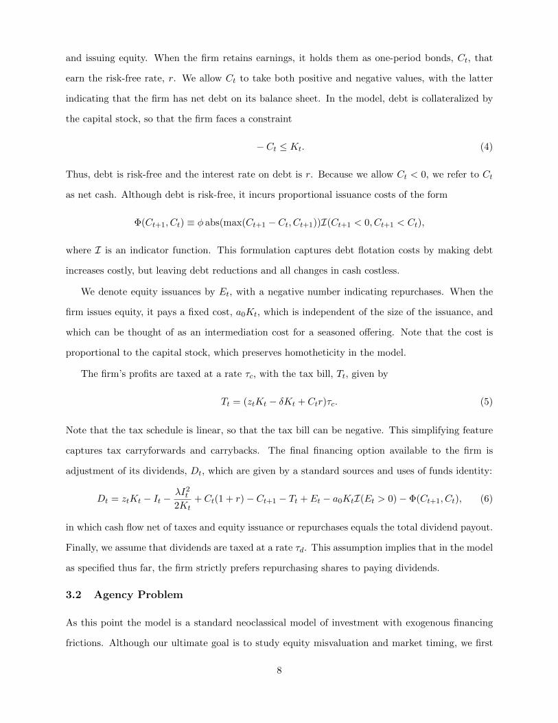
and issuing equity. When the firm retains earnings, it holds them as one-period bonds, Ct, that

earn the risk-free rate, r. We allow Ct to take both positive and negative values, with the latter

indicating that the firm has net debt on its balance sheet. In the model, debt is collateralized by

the capital stock, so that the firm faces a constraint

− Ct ≤ Kt. (4)

Thus, debt is risk-free and the interest rate on debt is r. Because we allow Ct < 0, we refer to Ct

as net cash. Although debt is risk-free, it incurs proportional issuance costs of the form

Φ(Ct+1, Ct) ≡ φ abs(max(Ct+1 − Ct, Ct+1))I(Ct+1 < 0, Ct+1 < Ct),

where I is an indicator function. This formulation captures debt flotation costs by making debt

increases costly, but leaving debt reductions and all changes in cash costless.

We denote equity issuances by Et, with a negative number indicating repurchases. When the

firm issues equity, it pays a fixed cost, a0Kt, which is independent of the size of the issuance, and

which can be thought of as an intermediation cost for a seasoned offering. Note that the cost is

proportional to the capital stock, which preserves homotheticity in the model.

The firm’s profits are taxed at a rate τc, with the tax bill, Tt, given by

Tt = (ztKt − δKt + Ctr)τc. (5)

Note that the tax schedule is linear, so that the tax bill can be negative. This simplifying feature

captures tax carryforwards and carrybacks. The final financing option available to the firm is

adjustment of its dividends, Dt, which are given by a standard sources and uses of funds identity:

Dt = ztKt − It −λI2t2Kt

+ Ct(1 + r)− Ct+1 − Tt + Et − a0KtI(Et > 0)− Φ(Ct+1, Ct), (6)

in which cash flow net of taxes and equity issuance or repurchases equals the total dividend payout.

Finally, we assume that dividends are taxed at a rate τd. This assumption implies that in the model

as specified thus far, the firm strictly prefers repurchasing shares to paying dividends.

3.2 Agency Problem

As this point the model is a standard neoclassical model of investment with exogenous financing

frictions. Although our ultimate goal is to study equity misvaluation and market timing, we first

8

need to consider the inherent agency problem associated with market timing. For a manager to take

advantage of misvalued equity, he needs to issue shares when equity is overvalued and repurchase

shares when it is undervalued. These transactions transfer wealth from the shareholders who trade

with the firm to those who do not. As such, market timing by managers implies that managers do

not maximize the value for all shareholders at all times.

We need to formalize this agency problem in a tractable way that lets us retain the rich speci-

fication of financing and investment, which is necessary for success in confronting the model with

data. To this end, we assume that managers maximize the value for a block of shares that constitute

a controlling position of the firm. We require that this controlling block not engage in any equity

transactions directly with the firm. This restriction is natural for a firm that issues and repurchases

shares to time the market because it would be disadvantageous for controlling block shareholders

to engage in any such share transactions with the firm. Although we assume the block contains a

fixed number of shares, we do not need to specify the exact size of this block, nor do we impose

the restriction that the size of the block remain the same across firms. In addition, we do not need

to make any assumptions about the identity of the shareholders in the controlling block; they can

sell the shares to new shareholders, who then take over the controlling stake. We do require that

the block not constitute all shareholders, and we thus assume that cumulated equity transactions

never cause the number of non-controlling shares to go to zero. Thus, there are always shareholders

available to take the opposite side of the equity transactions that benefit the shareholders in the

controlling block. The block must also be large enough to control the firm. Because the size of a

controlling block can be much smaller than 50% (La Porta, Lopez-de Silanes, and Shleifer 1999),

we do not need to assume a strict lower bound on the block size.

These assumptions on the size of the controlling block can effectively be viewed as implicit

restrictions on the model parameters that govern the size of equity transactions, with parameter

values that encourage net equity issuance shrinking the fractional size of the block, and vice versa.

To maintain tractability, we do not explicitly impose any such restrictions, but we later we examine

how well these assumptions hold at the estimated parameter values. Similarly, although controlling

shareholders clearly care about retaining control, for tractability, we do not allow the manager to

optimize over the size of the controlling stake. Again, we check the conditions under which control

9

might plausibly be lost, given our estimated parameter values.

We now show how these assumptions affect the managers’ maximization problem: first, in the

case of no misvaluation, and, second, in the case of misvaluation. In both cases, the fraction of

total shares outstanding owned by the controlling shareholders varies over time as the firm issues

and repurchases shares. We denote this fraction by ft. In the case of no misvaluation, the value of

the controlling block of shares can be written as follows:

V c(f0,K0, C0, z0) = maxKt,Ct,Et∞t=1

E0

( ∞∑t=0

βtft(1− τd)Dt

). (7)

The operator Et is the expectation operator with respect to the distribution of zt, conditional on

the information at time 0. As we assume that the controlling block does not engage in equity

transactions with the firm, its value does not incorporate payouts from repurchases.

We assume that the initial fraction held by the controlling block, f0, is such that the block always

maintains control of the firm. This assumption implies that f0 functions as a scaling parameter

that influences only the fraction of total dividends accruing to the controlling block. As such, we

can pull out f0 from the above infinite sum to obtain the following:

V c(f0,K0, C0, z0) = f0 maxKt,Ct,Et∞t=1

E0

( ∞∑t=0

βtftf0

(1− τd)Dt

). (8)

Define the value of the controlling block scaled by its fractional holding as:

V (K0, C0, z0, f0) ≡V c(f0,K0, C0, z0)

f0. (9)

We next show that V (K0, C0, z0, f0) can be expressed using a recursive formulation. Combining

together equations (8) and (9), we obtain:

V (K0, C0, z0, f0) = maxKt,Ct,Et∞t=1

(1− τd)D0 + E0

( ∞∑t=1

βtftf0

(1− τd)Dt

), (10)

where the initial dividend payment has been pulled out of the summation. The infinite sum (10)

can be expressed in recursive form as the Bellman equation:

V (K,C, z, f) = maxK′,C′,E

(1− τd)D + βE

(f ′

fV (K ′, C ′, z′, f ′)

), (11)

where a prime indicates a variable tomorrow and no prime indicates a variable today. Thus, we

have translated the problem of maximizing the value of the block shareholders into a recursive

specification that takes into account the evolution of the fraction of shares owned by the block.

10

The next proposition shows that it is possible to express f ′/f solely in terms of the current

state variables, (K,C, z).

Proposition 1 The fractional ownership of the controlling block evolves according to:

f ′

f=

V (K,C, z, f)−D(1− τd)V (K,C, z, f)−D(1− τd) + E

. (12)

The above expression has a very intuitive explanation. An equity issuance (E > 0) dilutes the

holdings of the controlling block and reduces its fractional ownership by a ratio determined by the

ex-dividend value of the firm. An equity repurchase (E < 0) has the opposing effect of concentrating

the fractional ownership of the controlling block.

Substituting (12) into (11) reveals that neither f nor f ′ has any impact on the firm’s optimal

policies. Thus, we can drop f from the expression for V (K,C, z, f) to obtain

V (K,C, z) = V (K,C, z, f). (13)

This simplification implies that the optimal policies of the firm and the value of the controlling

block scaled by its fractional holding are independent of the fractional holding itself. As such, our

model solution allows for variation in this controlling fraction across firms and over time.

3.3 Misvaluation

The next model ingredient is a misvaluation shock, ψ, that determines the ex-dividend equity value,

V ∗, at which equity transactions occur. In particular, V ∗ is a stochastic multiple of the ex-dividend

target equity value that the managers maximize for the controlling block defined in the previous

section. As these misvaluation shocks also affect the firm’s optimal policies, we now define this

target value as V (K,C,ψ, z). Note that V (K,C,ψ, z) differs from the fundamental value of the

firm that would be obtained in the absence of misvaluation. This difference arises because managers

actively optimize the value of the controlling block in response to misvaluation shocks. Thus, we

call V (K,C,ψ, z) “target value” because it is a function of the misvaluation term, ψ.

We write the value at which equity transactions occur, V ∗, as:

V ∗ = (V (K,C,ψ, z)−D(1− τd))ψ. (14)

When ψ = 1, the firm is valued correctly; when ψ < 1, the firm is undervalued; and when ψ > 1,

the firm is overvalued. This specification implies that misvaluation affects the price at which firms

11

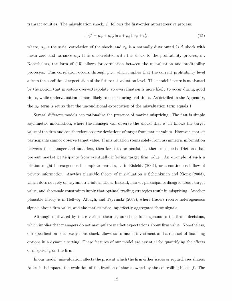
transact equities. The misvaluation shock, ψ, follows the first-order autoregressive process:

lnψ′ = µψ + ρzψ ln z + ρψ lnψ + ε′ψ, (15)

where, ρψ is the serial correlation of the shock, and εψ is a normally distributed i.i.d. shock with

mean zero and variance σψ. It is uncorrelated with the shock to the profitability process, εz.

Nonetheless, the form of (15) allows for correlation between the misvaluation and profitability

processes. This correlation occurs through ρzψ, which implies that the current profitability level

affects the conditional expectation of the future misvaluation level. This model feature is motivated

by the notion that investors over-extrapolate, so overvaluation is more likely to occur during good

times, while undervaluation is more likely to occur during bad times. As detailed in the Appendix,

the µψ term is set so that the unconditional expectation of the misvaluation term equals 1.

Several different models can rationalize the presence of market mispricing. The first is simple

asymmetric information, where the manager can observe the shock; that is, he knows the target

value of the firm and can therefore observe deviations of target from market values. However, market

participants cannot observe target value. If misvaluation stems solely from asymmetric information

between the manager and outsiders, then for it to be persistent, there must exist frictions that

prevent market participants from eventually inferring target firm value. An example of such a

friction might be exogenous incomplete markets, as in Eisfeldt (2004), or a continuous inflow of

private information. Another plausible theory of misvaluation is Scheinkman and Xiong (2003),

which does not rely on asymmetric information. Instead, market participants disagree about target

value, and short-sale constraints imply that optimal trading strategies result in mispricing. Another

plausible theory is in Hellwig, Albagli, and Tsyvinski (2009), where traders receive heterogeneous

signals about firm value, and the market price imperfectly aggregates these signals.

Although motivated by these various theories, our shock is exogenous to the firm’s decisions,

which implies that managers do not manipulate market expectations about firm value. Nonetheless,

our specification of an exogenous shock allows us to model investment and a rich set of financing

options in a dynamic setting. These features of our model are essential for quantifying the effects

of mispricing on the firm.

In our model, misvaluation affects the price at which the firm either issues or repurchases shares.

As such, it impacts the evolution of the fraction of shares owned by the controlling block, f . The

12

next proposition formally derives the evolution of this ratio in the presence of misvaluation.

Proposition 2 In the presence of misvaluation, the fractional holding of the controlling block

evolves according to the following:

f ′

f=

V (K,C,ψ, z)−D(1− τ)

V (K,C,ψ, z)−D(1− τ) + Eψ

. (16)

The above expression captures the effect of misvaluation on the evolution of the fractional holding

of the control block. When firms are overvalued, i.e., ψ > 1, they are able to obtain a given amount

of financing, E, by issuing a smaller number of shares, thus lessening the dilution of the controlling

block’s holding. On the other hand, when firms are undervalued, they are able to repurchase a

greater quantity of shares for a given amount of expenditures, E < 0, enabling the controlling block

to further concentrate its holdings.

Proposition 2 shows that under the assumption that the manager optimizes the value of a

controlling block of shareholders, the manager’s problem in the presence of misvaluation diverges

from the optimization problem previously detailed only in rate at which the fraction of shares held

by the controlling block evolves over time. As such, despite the nonstandard specification of the

Bellman equation, (11), our model framework is fully time consistent.

3.4 Price Impact

The model presented above entails uninformed investors transacting with the firm based on V ∗,

which incorporates an exogenous misvaluation shock. The model thus rests on the implicit assump-

tion that the firm manager knows more about the true value of the firm relative to these uninformed

investors. In this case, market participants are likely to infer from the firm’s equity repurchase and

issuance decisions that the share price may be overvalued or undervalued and then bid the price

down or up. See, for example, the evidence in Brockman and Chung (2001). More generally, a large

literature documents that firms can issue (repurchase) shares only at a discount (premium) to the

current price. For instance, Asquith and Mullins (1986) and Corwin (2003) find that SEOs occur

at discounts to market prices and that the discount increases with the size of the equity offering.

Similarly, a large literature following Vermaelen (1981) documents that firms announce repurchases

at a premium to the current share price. These findings imply that firms cannot transact at the

13

market price in the model, V ∗, but instead must transact at a price that takes into account the

potential price impact of their announced equity transaction. In terms of our model, price impact

therefore can therefore be viewed as a form of partial learning by these uninformed investors.

We model this price impact of equity transactions in a reduced-form manner by assuming that

firms transact as if the market value of the firm is given by V ∗/(1 + ν(E,K)), where:

ν(E,K) ≡ E

2K(νiI(E > 0) + νrI(E ≤ 0)) , νi, νr ≥ 0. (17)

This piecewise linear specification of the price impact term ν(E,K) implies that the firm faces a

discount from its market value when issuing shares (E > 0) and pays a premium when repurchasing

shares, consistent with the evidence noted above. Note that ν(E,K) is a function of the fraction

E/K. This assumption maintains homotheticity in the model and embodies the notion that the

price impact of an equity transaction depends on the size of transaction relative to firm size.1

This price impact affects the quantity of shares transacted by the firm, and thus the evolution

of the fractional holding of the controlling block, as follows:

Proposition 3 In the presence of misvaluation and price impact, the fractional holding of the

controlling block evolves according to the following:

f ′

f=

V (K,C,ψ, z)−D(1− τ)

V (K,C,ψ, z)−D(1− τ) + Eψ (1 + ν(E,K))

. (18)

The price impact implies that for a given equity issuance, E > 0, the firm must issue more shares

to offset the price impact as ν(E,K) > 0, leading to a larger reduction in the fractional holding

of the controlling block shareholders. Conversely, a firm can repurchase less shares for a given

amount E < 0, implying a smaller increase in the fractional holding of the controlling block. The

reduced-form specification of (17) assumes that if asymmetric information is the force behind the

price reaction, informational frictions prevent traders from completely inferring the firm manager’s

target valuation, V (K,C, z, ψ).

We can substitute the evolution of the fractional holding of the controlling block shown in

Equation (18) into Equation (11) to derive the following Bellman equation for the value of the

1For tractability, we also assume that the price impact does not affect the process for ψ in (15). Price impact inour model can therefore be thought of as the cash equivalent of the discount or premium the firm experiences in itsequity transactions. Because our estimates of price impact do not imply a large effect on the dilution or concentrationof blockholder value, this assumption likely has little impact on our results.

14

controlling block in the presence of misvaluation and price impact:

V (K,C,ψ, z) = maxK′,C′,E

(1− τd)D + β

(V −D(1− τd))ψ(V −D(1− τd))ψ + E(1 + ν(E,K))

E(V(K ′, C ′, ψ′, z′

)).

(19)

The above expectation is taken over the joint distribution of (ψ′, z′), conditional on (ψ, z). One

important implication of our motivation for the price impact term is the form the model takes in

the absence of misvaluation. As emphasized in Hennessy and Whited (2007), lemons’ premia and

other forms of price impact of can occur in the absence of misvaluation. In this case, by setting

ψ = 1 in (19), we obtain a standard neoclassical model with financing frictions.

It is not obvious that a solution to (19) exists, inasmuch as the discount factor need not always

be less than one. However, as in Bazdresch (2013), the following proposition allows the Bellman

equation (19) to be written with a constant discount factor.

Proposition 4 The solution to (19) is identical to the solution of

V (K,C,ψ, z) = maxK′,C′,E

(1− τd)D −

E(1 + ν(E,K))

ψ+ βE

(V(K ′, C ′, ψ′, z′

)). (20)

It is straightforward to show that (20) satisfies the conditions in Stokey and Lucas (1989) that are

necessary for the existence and uniqueness of a solution.

The above specification also highlights a helpful technical role that price impact plays in the

model. In the absence of price impact, the relative price of equity and dividends would be a linear

function of misvaluation, ψ. In addition, conditional on an equity transaction, equity transactions

and dividends offset each other one-for-one in the budget constraint, as shown in Equation (6). This

linearity implies that there would no interior solution for optimal equity issuances and repurchases

in the presence of misvaluation. The price impact term allows for an internal solution for equity

transactions because the marginal benefit of equity transactions declines with their size.

It is important to note that the Bellman equation (20) does not imply that the model contains

stochastic issuance costs, as in Eisfeldt and Muir (2012) or Bolton et al. (2013). This distinction

is important for three reasons. First, the misvaluation shock directly affects the price of equity

capital and thus affects both repurchases and issuances, instead of just issuance. Second, as we

show below, our model has the potential to generate realistic covariances between equity returns

and firm policies, whereas models with stochastic issuance costs cannot because they do not generate

15

sufficient equity variability. Finally, the misvaluation shock has no direct impact on the budget

constraint (6) that defines dividends, whereas stochastic issuance costs would.

Our model is, nonetheless, closely related to those in Gilchrist, Himmelberg, and Huberman

(2005) or Eisfeldt and Muir (2012). Gilchrist et al. (2005) examine equity issuance and investment

in a model with reduced-form bubbles in the price of equity. In contrast to their model, we allow

for equity to be both over- and under-priced relative to fundamentals, and we also allow for firms

to adjust on the savings margin, in addition to the investment margin. Eisfeldt and Muir (2012)

examine firm’s investment and saving decisions in the presence of stochastic issuance costs and

an aggregate productivity shock. However, they do not incorporate any deviations in the price of

equity from its fundamental value. Our model is also unique with respect to both of these models

in the distinction between dividends and repurchases.

3.5 Constant Returns to Scale Specification

Our model can be further simplified by taking advantage of its constant returns to scale nature,

and redefining all of the quantities in the model as a fraction of the capital stock, K. Define the

following scaled variables:

c ≡ C

K, d ≡ D

K, e ≡ E

K, i ≡ I

K, v(c, ψ, z) ≡ V (K,C,ψ, z)

K.

Then, by dividing all of the variables in (20) by K, we obtain the following Bellman equation:

v(c, ψ, z) = maxc′,e,i

(1− τd)d−

e(1 + ν(e, 1))

ψ+ βE

(v(c′, ψ′, z′

)(1− δ + i)

), (21)

and the constraints become:

d− e+ I(e > 0)a0 = z(1− τc)− i−λi2

2+ c(1 + r − rτc)− c′(1− δ + i) + δτc − Φ(c, c′), (22)

d ≥ 0 (23)

−c ≤ 1.

4 Optimal Policies

In this section, we analyze the first-order conditions for optimal financial and investment policies.

16

Equity and Dividends

We start with equity and dividend policy, holding optimal investment and net cash policy fixed.

The right-hand side of (22) is then also fixed. Let e∗ be the unconstrained best equity policy, which

is the optimal policy absent the constraint (23). We solve for e∗ by substituting (22) into (21),

differentiating with respect to e, and setting the result equal to zero. We also must ensure that e∗ is

large enough to warrant paying the fixed cost; that is, the payoff to equity holders if the firm issues

equity must exceed the payoff when it does not. Unconstrained optimal equity policy is given by:

e∗ =

(ψ(1− τd)− 1)/νi > 0 for ψ > 1/(1− τd) and (e∗ − a0)(1− τd)− e∗(1 + νie∗/2)/ψ < 0

(ψ(1− τd)− 1)/νr < 0 for ψ < 1/(1− τd)0 otherwise,

(24)

where the last expression on the first line of (24) is the extra optimality constraint that arises

from the fixed cost. This constraint implies an inaction region in which the firm neither issues nor

repurchases shares. Outside this region, for ψ sufficiently large, the firm wishes to issue equity, and

for ψ sufficiently small, the firm wishes to repurchase shares. The higher the parameters νi and

νr, the smaller the desired issuance and repurchasing activity. The dividend tax implies that when

ψ = 1, the optimal policy in the absence of the constraint (22) is to repurchase shares. If equity

policy is given by (24), desired dividends then are given by (22).

Of course, these first-order conditions ignore the constraint (23), which provides an important

link between the real and financial sides of the firm. If the first-order conditions in (24) produce

optimal dividends that are positive, then (24) holds exactly. However, if (24) implies that optimal

dividends are negative, the constraint binds, so that they are zero. Optimal equity issuance is then

given not by (24) but by the budget constraint (22). The policy implied by the budget constraint

always trumps the policy implied by the first-order condition when the two policies differ. Thus,

mispricing is not the sole determinant of equity policy: funding needs matter as well.

Table 1 contains a schematic that categorizes the possible combinations of optimal equity and

dividend policies. For brevity, we denote the right-hand side of the budget constraint (22) as b.

Then we have d − e + I(e > 0)a0 = b. The second column of Table 1 describes the equity policy

given by (24) alone, that is, e∗. The third column lists various possibilities for the value of the

budget constraint, b, relative to 0 and to e∗. The fourth and fifth columns list the optimal equity

17

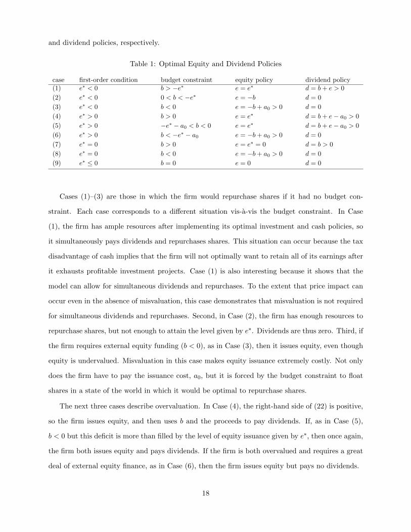
and dividend policies, respectively.

Table 1: Optimal Equity and Dividend Policies

case first-order condition budget constraint equity policy dividend policy(1) e∗ < 0 b > −e∗ e = e∗ d = b+ e > 0

(2) e∗ < 0 0 < b < −e∗ e = −b d = 0

(3) e∗ < 0 b < 0 e = −b+ a0 > 0 d = 0

(4) e∗ > 0 b > 0 e = e∗ d = b+ e− a0 > 0

(5) e∗ > 0 −e∗ − a0 < b < 0 e = e∗ d = b+ e− a0 > 0

(6) e∗ > 0 b < −e∗ − a0 e = −b+ a0 > 0 d = 0

(7) e∗ = 0 b > 0 e = e∗ = 0 d = b > 0

(8) e∗ = 0 b < 0 e = −b+ a0 > 0 d = 0

(9) e∗ ≤ 0 b = 0 e = 0 d = 0

Cases (1)–(3) are those in which the firm would repurchase shares if it had no budget con-

straint. Each case corresponds to a different situation vis-a-vis the budget constraint. In Case

(1), the firm has ample resources after implementing its optimal investment and cash policies, so

it simultaneously pays dividends and repurchases shares. This situation can occur because the tax

disadvantage of cash implies that the firm will not optimally want to retain all of its earnings after

it exhausts profitable investment projects. Case (1) is also interesting because it shows that the

model can allow for simultaneous dividends and repurchases. To the extent that price impact can

occur even in the absence of misvaluation, this case demonstrates that misvaluation is not required

for simultaneous dividends and repurchases. Second, in Case (2), the firm has enough resources to

repurchase shares, but not enough to attain the level given by e∗. Dividends are thus zero. Third, if

the firm requires external equity funding (b < 0), as in Case (3), then it issues equity, even though

equity is undervalued. Misvaluation in this case makes equity issuance extremely costly. Not only

does the firm have to pay the issuance cost, a0, but it is forced by the budget constraint to float

shares in a state of the world in which it would be optimal to repurchase shares.

The next three cases describe overvaluation. In Case (4), the right-hand side of (22) is positive,

so the firm issues equity, and then uses b and the proceeds to pay dividends. If, as in Case (5),

b < 0 but this deficit is more than filled by the level of equity issuance given by e∗, then once again,

the firm both issues equity and pays dividends. If the firm is both overvalued and requires a great

deal of external equity finance, as in Case (6), then the firm issues equity but pays no dividends.

18

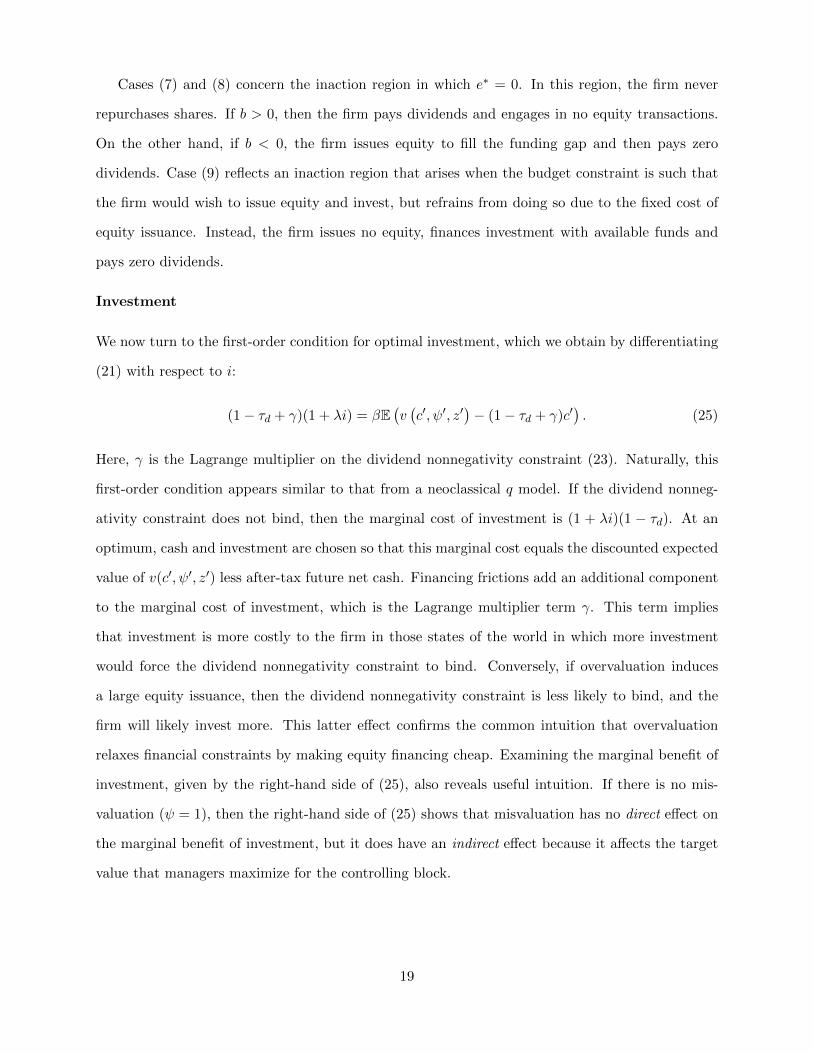
Cases (7) and (8) concern the inaction region in which e∗ = 0. In this region, the firm never

repurchases shares. If b > 0, then the firm pays dividends and engages in no equity transactions.

On the other hand, if b < 0, the firm issues equity to fill the funding gap and then pays zero

dividends. Case (9) reflects an inaction region that arises when the budget constraint is such that

the firm would wish to issue equity and invest, but refrains from doing so due to the fixed cost of

equity issuance. Instead, the firm issues no equity, finances investment with available funds and

pays zero dividends.

Investment

We now turn to the first-order condition for optimal investment, which we obtain by differentiating

(21) with respect to i:

(1− τd + γ)(1 + λi) = βE(v(c′, ψ′, z′

)− (1− τd + γ)c′

). (25)

Here, γ is the Lagrange multiplier on the dividend nonnegativity constraint (23). Naturally, this

first-order condition appears similar to that from a neoclassical q model. If the dividend nonneg-

ativity constraint does not bind, then the marginal cost of investment is (1 + λi)(1 − τd). At an

optimum, cash and investment are chosen so that this marginal cost equals the discounted expected

value of v(c′, ψ′, z′) less after-tax future net cash. Financing frictions add an additional component

to the marginal cost of investment, which is the Lagrange multiplier term γ. This term implies

that investment is more costly to the firm in those states of the world in which more investment

would force the dividend nonnegativity constraint to bind. Conversely, if overvaluation induces

a large equity issuance, then the dividend nonnegativity constraint is less likely to bind, and the

firm will likely invest more. This latter effect confirms the common intuition that overvaluation

relaxes financial constraints by making equity financing cheap. Examining the marginal benefit of

investment, given by the right-hand side of (25), also reveals useful intuition. If there is no mis-

valuation (ψ = 1), then the right-hand side of (25) shows that misvaluation has no direct effect on

the marginal benefit of investment, but it does have an indirect effect because it affects the target

value that managers maximize for the controlling block.

19

Net Cash

Let Ic be an indicator function that is one when the firm is issuing debt. We obtain the first-order

condition for net cash by differentiating (21) with respect to c′:

(1− δ + i− φIc) = βE(vc(c

′, ψ′, z′)(1− δ + i)). (26)

Next we use the envelope condition to eliminate vc(c′, ψ′, z′) from the problem. Let ξ be the

Lagrange multiplier associated with the collateral constraint (4). Substituting in the envelope

condition, vc(c, ψ, z) = (1 + r(1− τc) + φIc)(1 + γ + ξ), and rearranging gives:

(1− δ + i− φIc) = βE((1 + r(1− τc) + φI ′c)(1 + γ′ + ξ′)(1− δ + i)

). (27)

To interpret (27), we first set φ = 0, so that the (1 − δ + i) terms cancel. The right-hand side of

(27) is the expected discounted value of cash, which equals the after tax principal and interest on

net cash balances. The Lagrange multipliers γ′ and ξ′ then show that net cash is more valuable

when the dividend constraint or the collateral constraint is expected to bind. In particular, the

presence of ξ′ means that the firm adjusts net cash to avoid bumping up against the collateral

constraint. As is standard in dynamic investment models (e.g. Gamba and Triantis 2008), net cash

(equivalently, debt capacity) thus has value because it confers financial flexibility. If φ 6= 0, then

(27) shows that there is an inaction region for debt issuance. Because misvaluation is persistent, it

affects the constraints associated with dividends and net cash, and thus the Lagrange multipliers

γ′ and ξ′, which in turn affect the optimal cash holdings this period.

Numerical Policy Functions

In Figure 3, we plot the policy functions for investment, net cash, issuances/repurchases, and divi-

dends, which we denote as c′, i, e, d = h (c, ψ, z) . We parameterize the model using the estimates

from the late/large sample reported subsequently in Table 2.2

Panel A of Figure 3 depicts the optimal choices of net cash, investment, equity issuances/repurchases,

and dividends as a function of the misvaluation shock. The x-axis contains possible values of the

shock. It has a log scale because the shock is approximately lognormally distributed. A value

2Policy functions calculated with parameters from our other estimations are qualitatively similar.

20

of 1 indicates no misvaluation. To construct this panel, we have fixed the profit shock and the

current-period level of net cash at their respective sample means from a model simulation.

As expected, given the first-order conditions in (24), Panel A shows that the equity policy

function slopes upward, with an inaction region in the center that stems from the fixed issuance

cost. Outside of this inaction region, undervaluation results in repurchases, and overvaluation

results in issuance. More interesting is the contrast between the policy functions for investment

and net cash. The former is largely flat, except for a slight upward slope when the firm is issuing

equity. In contrast, the policy function for net cash largely tracks the policy function for equity

issuance. This contrast occurs because our parameter estimates indicate that investment is more

costly to adjust than net cash. Thus, the firm uses debt financing or dissaving for repurchases and

either hoards the proceeds from issuances as cash or uses the proceeds to pay down debt. Finally,

the policy function for dividends is also flat, except for a slight uptick for extreme overvaluation.

This pattern can also be understood in terms of Cases (4) and (5) in Table 1, in which desired

equity issuance is so high that there are proceeds left over to distribute to shareholders after all

other optimal policies have been funded.

Panel B Figure 3 depicts the response of investment, net cash, issuances/repurchases, and

dividends to the profitability shock, z. For this panel, we fix the level of ψ at 1/(1 − τd) and

the current-period level of net cash at the sample mean from a model simulation. In contrast to

the result in the Panel A, investment responds strongly and positively to the profitability shock

because the profitability shock is the one-period marginal product of capital. The response of

optimal net cash to the profitability shock is nonmonotonic. For most of the range of z, net cash

increases slightly. When z rises, the increase in the marginal product of capital implies that the

firm substitutes physical assets for financial assets. However, there is also a positive income effect

on net cash from a higher z, because costly external finance confers a flexibility benefit on net

cash. The income effect dominates for most of the range of z. For extremely high levels of z, the

flexibility benefit of higher net cash is negligible because the firm is flush with resources. Thus, the

firm increases net debt (decreases net cash) to finance capital accumulation.

Equity transactions do not vary with the profitability shock, remaining at 0 over the entire

range of z. When ψ = 1 < 1/(1− τd), (24) shows that zero equity transactions are optimal unless

21

the firm’s optimal cash and investment policies, together with the budget constraint (22), indicate

that the firm needs external equity financing. However, for the level of current cash underlying

Figure 3, the firm never optimally needs to fund investment with equity issuance. In contrast,

dividends do respond to the profitability shock, but only when it is high. In these states of the

world, the firm has more than enough internal funds to finance its optimal investment program, so

it pays the residual out to shareholders.

The main conclusions to be drawn from Figure 3 are as follows. First, investment is mostly

affected by shocks to profitability and not by equity market misvaluation. Second, net cash policy

is affected by both profitability and misvaluation shocks. Finally, equity issuance policy is affected

far more by misvaluation shocks than by profitability shocks. It is worth noting that these patterns

are in no way hardwired into the model because different arbitrary parameters can yield policy

functions with different shapes. For this reason, we analyze the model only for the parameter

values that we estimate, so that the results are empirically relevant.

5 Estimation and Identification

In this section, we first explain how we estimate the parameters of the model detailed in Section 3.

We then discuss our identification strategy.

5.1 Estimation

We estimate most of the structural parameters of the model using simulated method of moments

(SMM). However, we specify some model parameters separately. For example, we estimate the

risk-free interest rate, r, as the average real 3-month Treasury bill rate over the sample period

of interest. We set the corporate tax rate equal to 20%. This level is lower than the statutory

rate because we omit personal taxes on interest from the model. Finally, we set the tax rate on

dividends, τd equal to the difference between the statutory rates on dividends and capital gains.

We then estimate the following 12 parameters using SMM: the fixed equity issuance cost, a0; the

linear debt issuance cost, φ; the drift, standard deviation, and autocorrelation of the profitability

process, µ, σz and ρz; the quadratic adjustment cost parameter, λ; the standard deviation and

autocorrelation of the misvaluation process, σψ and ρψ; the market-timing penalties, νi and νr, the

22

correlation between the misvaluation and profitability shocks, ρzψ, and the depreciation rate, δ.

The SMM estimation proceeds as follows. First, we generate simulated data using the numerical

solution to the model. Specifically, we take a random draw from the distribution of(ε′z, ε

′ψ

),

conditional on (εz, εψ), and then compute v (c, ψ, z), (c′, e, i) = h (c, ψ, z) , and various functions of

v (c, ψ, z), c′, e, and i, such as Tobin’s q. We continue drawing values of(ε′z, ε

′ψ

)and using these

computations to generate an artificial panel of firms. Next, we calculate interesting moments using

both these simulated data and actual data. SMM then picks the model parameters that make the

actual and simulated moments as close as possible. The Appendix provides details.

One important issue for estimation is unobserved heterogeneity in our data from Compustat.

These firms differ along a variety of dimensions, such as technology and access to external finance. In

contrast, the only source of heterogeneity in our model is the individual draws of (εz, εψ). Therefore,

we remove the heterogeneity from the actual data, using fixed firm effects in the estimation of

variances and covariances. We calculate autocorrelation coefficients using the method in Han and

Phillips (2010), which controls for heterogeneity at the firm level.

This issue of heterogeneity implies that SMM estimates the parameters of an average firm, not

the average of the parameters across firms. These two quantities are not the same because the model

is nonlinear. Because it is often difficult to conceptualize an average firm in a large population of

firms over a long time span, we first examine subsamples of firms that are homogeneous along the

time and size dimensions, as in Figures 1 and 2. We examine separately the time periods before and

after the Jobs and Growth Tax Relief Reconciliation Act of 2003. Within these two time periods,

we analyze small and large firms, so that we end up with four groups of firms.

5.2 Identification

The success of this procedure relies on model identification, which requires that we choose moments

that vary when the structural parameters vary. In making these choices, we do not want to “cherry-

pick” moments because we want to understand what features of the data our model can and cannot

reconcile. Therefore, we examine the all of the standard deviations, as well as most of the means

and serial correlations, of all of the variables we can compute from our model: investment, profits,

equity issuances, equity repurchases, net cash, equity returns, and Tobin’s q. We construct our

simulated variables as follows. Net cash is c, investment is i, net saving is c′(1− δ + i)− c, equity

23

issuance is max(e, 0), repurchases are min(−e, 0), and returns are (ψ′v′)/(ψv)− 1.

We now describe and rationalize the 19 moments that we match. Of particular interest is

finding moments that can be used to identify the standard deviation and serial correlation of the

misvaluation shock, ρψ and σψ, as well as the correlation between the two shocks, ρzψ. Because

both the misvaluation shocks and profitability shocks affect firm policies, this task is difficult.

Of great help in this endeavor are the mean, standard deviation, and serial correlation of

operating profits, which are defined in the model as z. The only model parameters that induce any

variation in these three moments are the drift, residual standard deviation, and serial correlation of

the profitability shock, µ, σz, and ρz. Therefore, these three parameters can be pinned down using

only these three moments. Roughly speaking, with these three parameters pinned down, moments

related to the market value of the firm can be used to pin down ρψ, σψ, and ρzψ.

We use five moments related to market values. The first four are the standard deviation and

serial correlation of Tobin’s q and equity returns.3 All four moments are useful for identifying the

standard deviation and the serial correlation of the misvaluation process, σψ and ρψ. Intuitively, the

standard deviations of returns and Tobin’s q are strongly increasing in σψ. The serial correlation of

Tobin’s q increases with ρψ, while the serial correlation of returns decreases with ρψ because returns

are roughly the first difference of Tobin’s q, which is stationary in the model. The fifth moment

we use to identify misvaluation shocks is the slope coefficient from regressing equity issuance on

returns, which is generally increasing in ρzψ. Issuance is determined by both ψ and z, as is firm

value, so the higher the correlation between ψ and z, the more issuance covaries with returns.

Our next moments are the mean, serial correlation, and standard deviation of the rate of

investment, i. The standard deviation is useful for identifying the adjustment cost parameter, λ,

because higher λ produces less volatile investment. The serial correlation is primarily affected by

the smooth adjustment cost parameter, as well by the serial correlation of the profitability process,

ρz. The mean of investment is particularly useful for identifying the depreciation rate of capital,

as average investment is strongly increasing in this parameter.

The rest of the moments pertain to the firm’s financing decisions. We include the mean, serial

correlation, and standard deviation of the ratio of net cash to assets. The standard deviation of net

3We omit the means of Tobin’s q and equity returns because our model cannot capture rents to capital or theequity premium, which largely determine the means of these two variables, respectively.

24

cash decreases sharply with φ and is thus useful for its identification. We also include the mean and

standard deviation of the ratio of equity issuance to capital, the incidence of equity issuance, and the

mean and standard deviation of the ratio of repurchases to capital. These moments are useful for

identifying the equity issuance cost parameter, a0, the parameters penalizing equity transactions,

νi and νr. The incidence of issuance is particularly useful for identifying the standard deviation of

the misvaluation shock. Absent the misvaluation shock, the model can produce lumpy, infrequent

issuance that is used to fund investment. However, the frequency is much smaller than what is in

the data. The presence of the misvaluation shock helps bridge this gap.4

6 Results

This section presents estimates of the model from Section 3, as well as from an augmented model

that contains time-varying expected returns. For these first two estimations, we stratify the sample

by time period and firm size. We also report estimations from different industries.

6.1 Baseline Estimation

Panel A of Table 2 shows that the model fits the data surprisingly well. Across the four estimations,

only one third of the simulated moments are statistically significantly different from their data

counterparts, and only a handful are economically different. In addition, although we reject the

joint null that all of the model errors equal zero for the early samples and for the small firms in

the late sample, we cannot reject this null for the large firms in the late sample. This good fit is

remarkable, given that we have used many more moments than parameters in the estimation. The

model does an especially good job of matching all of the mean moments. In particular, the model

comes close to matching the high net cash of the small firms in the latter part of the sample. The

model also reconciles the standard deviations of most of the variables. Here, the ability of the model

to match the standard deviation of profits is important. Otherwise, if the model could not generate

sufficient variability in profits, this shortcoming would put substantial weight on misvaluation to

generate sufficient variability in firm policies. The model struggles with only a few features of

4We omit moments related to dividends. As with all investment-based models of financing (e.g. Hennessy andWhited 2005, 2007), the model-implied variance of dividends far exceeds the smoothness observed in the data. If weuse dividend moments in the estimation, this model failure causes many moments to be poorly matched. Therefore,any counterfactuals constructed using the poorly fitting simulated moments produce inaccurate inferences.

25

the data. The serial correlations of net cash and returns are too high, and the serial correlation

of Tobin’s q is too low. Also, the means of repurchases in the late period are too low, and the

standard deviation of investment in three of the four samples is too low.

Panel B of Table 2 presents the parameter estimates we obtain from each of our four samples.

Most of the parameters are statistically significant. Two exceptions are the estimates of the equity

issuance cost parameter (a0) from the late period. This result is not surprising, given the rise of

the practice of shelf registration of equity offerings (Gao and Ritter 2011). The other exceptions

are three of the estimates of the shock correlation parameter, ρzψ, and all of the estimates of the

debt issuance cost parameter, φ. Although we cannot estimate φ precisely, the cost of debt issuance

does play a helpful role in constraining the volatility of net cash holdings.

More importantly, for all four samples, the standard deviations of the misvaluation shocks are

highly statistically significant, ranging from 0.21 to 0.29. To interpret these magnitudes, it is

important to remember that these figures are for ln(ψ), not for the level of ψ. Thus, the standard

deviation estimates are of the same order of magnitude as return standard deviations, which in

our four samples run from 42% to 55%. We conclude that a great deal, but by no means all of

the variability in market values fails to reflect the manager’s view of fundamentals. Finally, note

that the estimates of the serial correlation of the process for ln(ψ) are all low and insignificantly

different from zero. This result implies that the standard deviation of the innovation to the process

for ln(ψ) roughly equals the standard deviation of ln(ψ) itself.

The economic magnitudes of many of the other parameters are plausible. The estimates of

the adjustment cost parameters correspond to the range of estimates of the coefficient on Tobin’s

q reported in, for example, Erickson and Whited (2012). Two parameters that are difficult to

interpret are νi and νr, so we gauge their economic magnitudes by setting them to zero, calculating

the dilution or concentration of the value of the controlling block that occurs, and then comparing

these figures to the dilution or concentration that occurs, given the estimated values of νi and

νr. These figures are reasonable. For example, according to the late-large estimation, an equity

issuance of 1% of firm value has a dilution effect for controlling shareholders equal to an issuance of

1.09% of firm value in a frictionless setting with no νi term. These dilution effects range from 1.02%

to 1.05% for the other three samples. The figures for repurchases imply that the concentration of

26

the holdings of controlling shareholders ranges from 0.78% to 0.97% for a 1% equity repurchase.

In sum, although we find a sizable amount of perceived misvaluation, these parameter estimates

indicate that potential adverse market responses limit managers’ ability to take advantage of it.

Recall that we have not restricted the parameter values to ensure that the size of the controlling

block does not become either too small or so large that it encompasses all shareholders. To address

these possibilities, we calculate how many years it would take for either of these two scenarios to

occur, given our estimated parameter values. For the early/small sample, average issuance exceeds

average repurchases, so the concern is that the controlling stake will be diluted. We use model

simulations to calculate that if would take over 100 years for a 50% ownership stake to be diluted

in half. For the other three samples, because average repurchases exceed issuance, the concern

is that the controlling stake would grow to comprise the entire firm. We calculate that for an

initial controlling stake of 50%, it would take between 40 and 100 years for this scenario to occur,

depending on the sample. These time spans are sufficiently long to support our assumptions about

the fixed size of the controlling block.

6.2 Pricing Kernel

We now ask whether our estimates of the variance of the misvaluation shock are simply picking

up movements in rational expected returns. To this end, we add an aggregate productivity term

to our model that is calibrated to match the duration and severity of expansions and recessions in

the United States and an associated pricing kernel. See the Appendix for details. Table 3 presents

our estimates of this augmented model. The augmented model fits most of the moments better,

which is not surprising, given that the augmented model contains an extra shock. Interestingly,

the estimates for the standard deviation of the misvaluation shock are still significantly different

from zero. Compared to the estimates in Table 2, they are nearly the same for the early period

and slightly higher for the late period, compared to baseline model. Thus, time-varying expected

returns cannot account for the levels of the misvaluation shock standard deviation.

6.3 Industry Estimation

The parameter estimates we obtain are for an average firm, not an average parameter across firms.

Therefore, we now estimate the model using data from homogeneous groups of firms that are

27

stratified by two-digit SIC industry. This exercise provides a stricter test of the model’s ability to

rationalize the data from very different types of firms.

Because our highly nonlinear estimations require a great deal of data for identification, we

choose the eight two-digit SIC codes with the most data points. SIC13 is oil and gas extraction;

SIC20 is food products; SIC28 is chemicals and allied products; SIC35 is machinery and computer

equipment; SIC36 is electronic and electrical equipment; SIC38 is measuring instruments; SIC50 is

wholesale trade; and SIC73 is business services.

We first present the moment estimates. For brevity, Figure 4 displays our results from matching

an important subset of moments: the means of the four policy variables in our model, which are

investment, net cash, equity issuances, and repurchases. Each panel in Figure 4 corresponds to a

different moment, with the x-axes containing the simulated moments and the y-axes containing the

data moments. Each pair of data moment and corresponding simulated moment is then labeled by

the relevant industry SIC code.

Panels A and B show that the model does an excellent job of matching average net cash

and investment. These moment pairs line up nicely along their respective 45 lines, and none of

these pairs represent a significant model error. This result is particularly strong, given the large

differences in the moments across industries. For example, oil and gas extraction has high net

debt of approximately 25% of assets, while business services has high net cash of approximately

3% of assets. As seen in Panel C, the model does not do as good a job of matching average equity

issuance. Although the model can capture the wide difference between the low equity issuance

in food and the very high equity issuance in oil and gas, three of eight pairs of moments are

statistically significantly different from each other. Panel D shows that the model does a somewhat

worse job with average repurchases. Only two of these moment pairs are insignificantly different

from each other. Nonetheless, the model does capture the “spread” observed in the repurchase

moment conditions across industries.

Table 4 contains the parameter estimates. We concentrate on the estimates of the standard

deviation a of the misvaluation shock. The industries with the lowest variance shocks are SIC20

(food products), SIC50 (wholesale trade), and SIC 38 (measuring instruments). The industries with

the highest variance shocks are SIC13 (oil and gas extraction), SIC35 (machinery and computer

28

equipment), SIC 36 (electronic equipment), and SIC73 (business services). It is useful to compare

these estimates with other measures of misvaluation. Unfortunately, the misvaluation of an entire

group of firms is hard to gauge. Nonetheless, we find it plausible that firms in high R&D industries

are more opaque, and thus more likely to suffer from misvaluation. The bottom row of Table 4

contains average R&D for the firms in each industry. Interestingly, the lowest R&D industries

(food and wholesale) have the lowest variance misvaluation shocks, which are also statistically

insignificant. Except for oil and gas extraction, which does negligible R&D, the highest R&D

industries also have the highest variance misvaluation shocks. One obvious explanation for the oil

and gas industry is that the exploration business is extremely risky and the oil reserves of these

companies are hard to value. These results thus constitute a useful external model validation

exercise that lends credibility to the interpretation of ψ as a misvaluation shock, as opposed to

some other source of variability.

7 Counterfactuals

We now quantify the effects of misvaluation via counterfactual exercises. First, in Figure 5 we

measure the change in firm policies when we alter the standard deviation of the misvaluation shock

process. To construct this figure, we parameterize the model with the late-large estimates in Table

2 because this is the sample on which the model fits best, so our counterfactuals will be most

empirically relevant.5 We then solve the model 20 times, each time corresponding to a different

value of σψ, with the rest of the parameters held at their estimated values. For each model solution,

we simulate 150,000 firm-year observations, and then compute the averages of five variables.

Panel A of Figure 5 plots repurchases and equity issuance as a function of the standard devi-

ation of the misvaluation shock, σψ. In both cases, we average in observations with zero activity.

Not surprisingly, average equity issuances and repurchases increase with the misvaluation shock

standard deviation. To understand whether the increase in issuance is due to size or frequency, we

also plot the incidence of equity issuance. Interestingly, average incidence rises almost parallel with

average issuance, which means that the average size of an issuance remains roughly constant. Only

the frequency increases with misvaluation shock standard deviation.

5 The results using the other model parameterizations are qualitatively similar.

29

In Panel B of Figure 5, we plot average net cash and average investment as a function of σψ. Net

cash is much higher for firms that face higher standard deviation misvaluation shocks. Although

average investment is also higher, this effect is much more modest. For reference, we also plot the

level of investment that would result from a frictionless neoclassical investment model with the

same profitability shock process, depreciation rate, and investment adjustment costs. Interestingly,

we find that firms overinvest relative to this level, except at the lowest misvaluation shock volatility.

This result is interesting because it shows that in the model misvaluation shocks allow firms to issue

equity when the existence of equity issuance costs would make this source of financing prohibitively

expensive, that is, misvaluation alleviates financial constraints. We find that this effect does not

result in the same level of investment that would occur in a frictionless environment. Instead, the

resulting level of investment is somewhat higher.

Panel C of Figure 5 plots average firm fundamental value, v as a function of σψ, where we

have normalized the value with no misvaluation to be one so that the plot isolates the value of

timing. The effect of σψ is modest, especially for low shock standard deviations. One question

we can answer from this plot is how much controlling shareholders’ value would be lost if the

shock standard deviation were zero instead of its estimated value of 0.29. Equivalently, how much

value would be lost if the manager followed the optimal policies of a firm that experienced less

(or no) misvaluation, but worked in a firm subject to misvaluation. We find that the controlling

shareholders would lose 3% of their equity value.6 This figure is likely an upper bound for the

actual amount of lost value. When we change the misvaluation shock standard deviation, we do so

holding all other parameters constant. However, it is unlikely that the market response to equity

issuance and repurchases (as captured by the parameters νi and νr) would remain the same in a

low misvaluation environment. Indeed, these parameters would likely be somewhat smaller and

equity transactions would be less constrained. More liberal equity policies would then attenuate

the drop in the value of controlling shareholders’ equity.

To understand the economic mechanisms behind this result, we examine the immediate impact

of misvaluation shocks by calculating impulse response functions. Once again, we parameterize the

model using the estimates from the large firms in the late period. This exercise differs from our

6The corresponding figures for our other three samples are between 2.1% and 3%.

30

comparative statics exercises in which we change a model parameter and then examine its impact

on average firm policies. Instead, we are looking at the immediate response of a single variable to

an actual realization of a shock. Calculating an impulse response function with real data requires

estimating, inverting, and orthogonalizing a vector autoregression because the shocks that drive the

variables of interest are unobservable. However, in our simulated data we do observe our shocks,

so to calculate our impulse response functions, we simply regress our variables of interest on each

of our two shocks, which we standardize and orthogonalize using a Cholesky decomposition.

The results are in Figure 6. The y-axis in each panel contains the change in the variable of

interest in response to a one standard deviation shock. The x-axis is time since the shock realization.

The most striking result is in Panel A, which depicts net cash balances. A one standard deviation

misvaluation shock raises net cash balances by about 2% of assets. This substantial effect dies out

only by half after five years. As shown in Panels B–D, a one standard deviation misvaluation shock

also has important effects on issuances and repurchases, but not on investment.

The effects of the profit shock are noticeably different in magnitude. First, a one standard

deviation profit shock has a large negative effect on average net cash balances, as firms substitute

out of financial capital and into physical capital when the latter becomes more productive. For firms

with positive net debt, this response simply represents the use of debt finance to fund investment.

Interestingly, this effect dies out rapidly. Next, we find that issuance and repurchases respond

only weakly to the profit shocks. In the case of issuance, a one standard deviation shock does not

induce such a large investment that the firm wishes to pay the fixed issuance cost to finance the

investment with equity. In contrast, profit shocks have a much stronger effect on investment than

do misvaluation shocks.

External validity

Finally, we conduct an informal “out-of-sample” test of the validity of our model, in the sense that

we want to ascertain whether it can reconcile patterns in the data that were not used to estimate

it. In particular, given our interest in market timing, we want to ascertain whether our model

can replicate the correlations between equity returns and a variety of different variables. Table 5

contains the results from this comparison. We do separate calculations for the four samples from

Table 2: early/small, early/large, late/small, and late/large, with Panel A containing results from

31

a model with the estimated variances of the misvaluation shocks and with Panel B containing the

results for no misvaluation. The actual data correlations are correlations between the aggregate

variables depicted in Figures 1 and 2. The simulated correlations are from data simulated from the

model, given the four different parameterizations.

Panel A shows that for all four samples, we match the signs of the correlations between returns

and investment, net saving, equity issuance, and repurchases. We also match many of the actual

magnitudes of the correlations, although our model captures only about half of the extremely high

correlation between net saving and returns for the small firms in the late sample. However, this

large correlation is primarily driven by the 2007–2009 financial crisis. Our model does not do as

good a job at matching the signs of the correlations between returns and dividends, which is not

surprising because we have no moments related to dividends in our estimation. Nonetheless, given

that we only use a moment related to one out of these five correlations (returns versus issuance) in

our estimation, our ability to replicate other correlations bolsters confidence in the model.

Panel B examines the role of misvaluation in generating these correlations. For this panel, we set

the variance of the misvaluation shocks to near zero. We find that even without misvaluation, the

model can generate substantial correlations between returns and investment or returns and saving,

especially in the early sample. What the model without misvaluation cannot do is generate sizable

correlations between returns and equity transactions, except for repurchases in the early/large

sample. In the late sample, the model without misvaluation also cannot generate even moderate

correlations between returns and savings. We conclude that the misvaluation shocks are essential

for making sense of the correlations between returns, issuances, and repurchases in Figures 1 and

2. Misvaluation shocks are also helpful in reconciling about half of the high correlation between

saving and returns observed in the late part of the sample.

8 Conclusion

In this paper, we quantify the extent to which nonfundamental movements in the price of a firm’s

stock affect its various policies. Although this topic has been addressed by a large number of

studies, we approach the problem in a new way—structural estimation—with the intent of adding

quantitative results to this body of literature. We develop a framework for firm optimization

32

decision in the presence of misvaluation. Building on this framework, we estimate a version of

a constant returns neoclassical investment model in which equity financing is costly, the firm can

accumulate cash and issue debt, and, most importantly, equity values can be subject to misvaluation

shocks. In the model, firms naturally issue equity when it is overvalued and repurchase equity

when it is undervalued. Depending on the model parameters, the funds flowing to and from these

activities can come from either changes in (net) cash balances or changes in investment, or both.

We find that non-fundamental movements in equity prices (misvaluation) are sizable. Our

counterfactual exercises show misvaluation shocks directly induce firms to issue and repurchase

equity, but the proceeds from these issuances and the funds from these repurchases flow into and

out of net cash balances. The immediate impact on real investment expenditures is small. This

result echoes the descriptive findings in McLean (2011) that firms tend to hoard the proceeds from

equity issuances. These higher net cash balances provide firms with more financial flexibility, which

in turn adds to the equity value of controlling shareholders. In short, misvaluation has large effects

on financial policies, especially equity transactions, much smaller effects on real investment policies,

and modest valuation effects.

One admitted drawback of our approach is our modeling of misvaluation shocks as exogenous.

This modeling choice is necessary for tractability, which allows us to examine the interesting ques-

tion of market timing quantitatively. However, this choice makes it difficult to answer questions

related to managers’ manipulation of share prices. If managers do attempt to misguide sharehold-

ers, then their reactions to mispricing might differ from those produced by our model. Examining

this type of framework is an interesting avenue for future research.

33

References

Abel, A. B., and J. C. Eberly. 1994. A Unified Model of Investment Under Uncertainty. AmericanEconomic Review 84:1369–1384.

Alti, A., and J. Sulaeman. 2011. When do High Stock Returns Trigger Equity Issues? Journal ofFinancial Economics 103:61–87.

Alti, A., and P. Tetlock. 2013. How Important Is Mispricing? Journal of Finance, forthcoming.

Asquith, P., and D. W. Mullins, Jr. 1986. Equity issues and offering dilution. Journal of FinancialEconomics 15:61–89.

Baker, M., and J. Wurgler. 2012. Behavioral Corporate Finance: An Updated Survey. In G. Con-stantinides, M. Harris, and R. Stulz (eds.), Handbook of the Economics of Finance, vol. 2. North-Holland: Elsevier.

Bazdresch, S. 2013. Financial lumpiness and investment. Journal of Economic Dynamics andControl .

Bolton, P., H. Chen, and N. Wang. 2013. Market timing, investment, and risk management. Journalof Financial Economics 109:40–62.

Brockman, P., and D. Y. Chung. 2001. Managerial timing and corporate liquidity: evidence fromactual share repurchases. Journal of Financial Economics 61:417–448.

Corwin, S. A. 2003. The determinants of underpricing of seasoned equity offers. Journal of Finance58:2249–2279.

DeAngelo, H., L. DeAngelo, and T. M. Whited. 2011. Capital structure dynamics and transitorydebt. Journal of Financial Economics 99:235–261.

Duffie, D., and K. J. Singleton. 1993. Simulated Moments Estimation of Markov Models of AssetPrices. Econometrica 61:929–52.

Eckbo, B. E., R. W. Masulis, and Oyvind. Norli. 2007. Security Offerings, Handbook of CorporateFinance: Empirical Corporate Finance, E. Eckbo. In B. E. Eckbo (ed.), Handbook of CorporateFinance: Empirical Corporate Finance. Amsterdam: Elsevier.

Eisfeldt, A., and T. Muir. 2012. Aggregate Issuance and Savings Waves. Manuscript, UCLA.

Eisfeldt, A. L. 2004. Endogenous Liquidity in Asset Markets. Journal of Finance 59:1–30.

Erickson, T., and T. M. Whited. 2002. Two-step GMM estimation of the errors-in-variables modelusing high-order moments. Econometric Theory 18:776–799.

Erickson, T., and T. M. Whited. 2012. Treating measurement error in Tobin’s q. Review of FinancialStudies 25:1286–1329.

Gamba, A., and A. Triantis. 2008. The value of financial flexibility. Journal of Finance 63:2263–2296.

Gao, X., and J. Ritter. 2011. The Marketing of Seasoned Equity Offerings. Journal of FinancialEconomics 97:33–52.

Gilchrist, S., C. P. Himmelberg, and G. Huberman. 2005. Do stock price bubbles influence corporateinvestment? Journal of Monetary Economics 52:805 – 827.

Gomes, J. F. 2001. Financing Investment. American Economic Review 91:1263–1285.

34

Graham, J. R., and C. R. Harvey. 2001. The theory and practice of corporate finance: Evidencefrom the field. Journal of Financial Economics 60:187–243.

Han, C., and P. C. B. Phillips. 2010. GMM Estimation for Dynamic Panels with Fixed Effects andStrong Instruments at Unity. Econometric Theory 26:119–151.

Hayashi, F. 1982. Tobin’s marginal q and average q: A neoclassical interpretation. Econometrica50:213–224.

Hellwig, C., E. Albagli, and A. Tsyvinski. 2009. Information Aggregation and Investment Decisions.Manuscript, Harvard University.

Hennessy, C. A., and T. M. Whited. 2005. Debt dynamics. Journal of Finance 60:1129–1165.

Hennessy, C. A., and T. M. Whited. 2007. How costly is external financing? Evidence from astructural estimation. Journal of Finance 62:1705–1745.

Ingram, B. F., and B.-S. Lee. 1991. Simulation and Estimation of Time Series Models. Journal ofEconometrics 47:197–205.

Jenter, D., K. Lewellen, and J. B. Warner. 2011. Security Issue Timing: What Do Managers Know,and When Do They Know It? Journal of Finance 66:413–443.

Kyle, A. S. 1985. Continuous auctions and insider trading. Econometrica 53:1315–1335.

La Porta, R., F. Lopez-de Silanes, and A. Shleifer. 1999. Corporate Ownership around the World.Journal of Finance 54:471–517.

Matvos, G., and A. Seru. 2013. Resource Allocation within Firms and Financial Market Dislocation:Evidence from Diversified Conglomerates. Review of Financial Studies Forthcoming.

McKeon, S. 2013. Firm-Initiated versus Investor-Initiated Equity Issues. Manuscript, Universityof Oregon.

McLean, R. D. 2011. Share issuance and cash savings. Journal of Financial Economics 99:693 –715.

Scheinkman, J. A., and W. Xiong. 2003. Overconfidence and speculative bubbles. Journal ofPolitical Economy 111:1183–1220.

Shiller, R. J. 1981. Do Stock Prices Move Too Much to be Justified by Subsequent Changes inDividends? The American Economic Review 71:421–436.

Skinner, D. J. 2008. The evolving relation between earnings, dividends, and stock repurchases.Journal of Financial Economics 87:582–609.

Stokey, N. L., and R. E. Lucas. 1989. Recursive Methods in Economic Dynamics. Cambridge, MA:Harvard University Press.

Taylor, L. A. 2010. Why are CEOs rarely fired? Evidence from structural estimation. Journal ofFinance 65:2051–2087.

Vermaelen, T. 1981. Common stock repurchases and market signalling. Journal of FinancialEconomics 9:139–183.

Yang, B. 2013. Capital Structure with Heterogeneous Beliefs and Market Timing. Journal ofCorporate Finance 22:254–277.

35

Appendix

This Appendix contains the proofs of Propositions 1–4, the derivation of µψ, the model that contains

time-varying expected returns, and an outline of the estimation procedure.

Proof of Proposition 1

Let Q denote the number of shares outstanding for the firm, and let F denote the number of shares

in the controlling block. As noted above, F is a constant. The fraction of shares in the controlling

block is then given by f = FQ . The ex-dividend price per share of the firm equals V (K,C,z)−D(1−τd)

Q .

Consider an equity issuance of E. Such an issuance will involve an increase in the quantity of shares

outstanding of N = QEV (K,C,z)−D(1−τd) , which follows from dividing the value of the issuance by the

share price. Thus, the quantity of shares outstanding evolves according to the following equation:

Q′ = Q+QE

V (K,C, z)−D(1− τd). (A.1)

Some algebra reveals:

Q′

Q=V (K,C, z)−D(1− τd) + E

V (K,C, z)−D(1− τd). (A.2)

Following the definition of the fraction of shares in the controlling block,

f ′

f=Q

Q′. (A.3)

This expression reflects the fact that an increase in the quantity of shares outstanding will reduce

the fractional ownership of the controlling block. Substituting (A.3) into (A.2) and taking the

inverse, one obtains:

f ′

f=

V (K,C, z)−D(1− τd)V (K,C, z)−D(1− τd) + E

. (A.4)

Thus, the evolution of the fraction of shares held by the controlling block can be written solely in

terms of firm value, dividends and equity issuance.

Proof of Proposition 2

Misvaluation affects the price at which firms transact shares, which is now a function of V ∗. We

start with the number of shares in an equity transaction, which is:

N =QE

V ∗=

QE

ψ(V (K,C,ψ, z)−D(1− τd)). (A.5)

36

We now obtain the following expressions for the evolution of the fraction of shares held by the

controlling block.

Q′ = Q+QE

ψ(V (K,C,ψ, z)−D(1− τd)),

Q′

Q=

ψ(V (K,C,ψ, z)−D(1− τd)) + E

ψ(V (K,C,ψ, z)−D(1− τd)),

f ′

f=

ψ(V (K,C,ψ, z)−D(1− τd))ψ(V (K,C,ψ, z)−D(1− τd)) + E

,

f ′

f=

V (K,C,ψ, z)−D(1− τd)V (K,C,ψ, z)−D(1− τd) + E

ψ

. (A.6)

Proof of Proposition 3

The price impact term changes the price at which firms can transact shares as a function of the size

of the transaction. As above we need to express the number of shares in a given equity transaction:

N =QE(1 + ν(E,K))

V ∗(K,C,ψ, z)(A.7)

We can now use equation (A.7) and proceed as above to derive the evolution of the fraction of

shares held by the controlling block.

Q′ = Q+E(1 + ν(E,K))Q

ψ(V (K,C,ψ, z)−D(1− τd)),

Q′

Q=

ψ(V (K,C,ψ, z)−D(1− τd)) + E(1 + ν(E,K))

ψ(V (K,C,ψ, z)−D(1− τd)),

f ′

f=

ψ(V (K,C,ψ, z)−D(1− τd))ψ(V (K,C,ψ, z)−D(1− τd)) + E(1 + ν(E,K))

,

f ′

f=

V (K,C,ψ, z)−D(1− τd)V (K,C,ψ, z)−D(1− τd) + E

ψ (1 + ν(E,K)).

Proof of Proposition 4

Let V be a solution to equation (19), with corresponding policy functions D and E. Then one

obtains from (19):

V (K,C,ψ, z) = D(1−τd)+βψ(V − D(1− τd))

ψ(V − D(1− τd)) + E + ν(E,K)

∫V(K ′, C ′, ψ′, z′

)dg(ε′ψ, ε

′z,∣∣ εψ, εz) .

37

Rearranging the dividend term and dividing the numerator and denominator of the left hand side

by ψ gives

V (K,C,ψ, z)−D(1−τd) = β(V − D(1− τd))

(V − D(1− τd)) + Eψ + ν(E,K)

ψ

∫V(K ′, C ′, ψ′, z′

)dg(ε′ψ, ε

′z,∣∣ εψ, εz)).

(A.8)

Next, divide(A.8) throughout by V (K,C,ψ, z) − D(1 − τd) and multiply by V (K,C,ψ, z) −

D(1− τd) + E/ψ + ν(E,K)/ψ to obtain

V (K,C,ψ, z)− D(1− τd) +E

ψ+ν(E,K)

ψ= β

∫V (K ′, C ′, ψ′, z′) dg

(ε′ψ, ε

′z,∣∣ εψ, εz) ,

Thus V , D, and E also solve equation (20).

Conversely, let V be a solution to equation (20), with corresponding policy functions D and E.

One can use a similar approach to the above to show that V , D, and E also solve (19).

Derivation of µψ

Define the following matrices:

Y =

[ln zlnψ

], C =

[µzµψ

], R =

[ρz 0ρzψ ρψ

], ε =

[εzεψ

,

]Σ =

[σ2z 00 σ2ψ

].

Then, the joint transition equation can be written as the following VAR(1):

Yt+1 = C +RYt + ε, ε ∼ N(0,Σ).

The unconditional mean of Y is given by the following expression:

E[Y ] = (I2 −R)−1C,

where In denotes a identity matrix of order n. The unconditional variance of Y is given by:

Vec(Var(Y )) = [(I4 − (R⊗R)]−1 Vec(Σ),

where Vec denotes the vectorization operator and ⊗ denotes the Kronecker product. For notational

convenience, let M = [(I4 − (R⊗R)]−1. One can then derive the unconditional mean and variance

38

of Y (2) = lnψ as:

E[lnψ] =1

(1− ρz)(1− ρψ)(ρzψµz + (1− ρz)µψ) ,

Var(lnψ) = M(4, 1)σ2z +σ2ψ

(1− ρ2ψ),

where M(4, 1) denotes the (4, 1)th element of the matrix M . The restriction that the unconditional

expectation of the misvaluation term equals one implies that

lnE[ψ] = 0, ⇒ E[lnψ] + 0.5Var(lnψ) = 0.

Some algebra then reveals that

µψ = −

[1

2(1− ρψ)M(4, 1)σ2z +

σ2ψ2(1 + ρψ)

+ρzψµz1− ρz

].

Time-Varying Expected Returns

Let xt be an aggregate productivity variable that takes one of two values, xl, xh. Let xl denote

a recessionary state and xh an expansionary state (xh > xl). The probability of remaining in

a recessionary state is given by pl, and the probability of remaining in an expansionary state

is given by ph. This implies expected durations of recessions and expansions of 1/(1 − pl) and

1/(1− ph), respectively. In addition, we impose the restriction that the unconditional expectation

of the aggregate productivity shocks equals 1 so that average profits remains unchanged from the

previous model.7

The expected return varies with aggregate productivity xt. Denote the conditional expected

return as

βm(x, x′).

Following the production-based asset pricing literature, the time-varying expected return can be

parameterized as a function of current and future aggregate productivity. Thus,

lnm(x, x′) = m0 +m1(x′ − x).

7Formally, this imposes the restriction that xh1−pl

2−ph−pl+ xl

1−ph2−ph−pl

= 1.

39

Economic reasoning suggests that investors place a higher valuation on assets that payoff in bad

states of the world. This imposes the requirement that m1 < 0. In order to ensure that aver-

age discount rates remain unchanged from the model without aggregate shocks, we require that

E[m(x, x′)] = 1.8

Given these assumptions, the expanded model can be written as follows:

v(c, ψ, z, x) = maxc′,e,i

d(1− τd)−

e(1 + ν(e, 1))

ψ+ βE

(m(x, x′)v(c′, ψ′, z′, x′)(1− δ + i)

)d− e+ I(e > 0)a0 = zx(1− τc)− i−

λi2

2+ c(1 + r − rτc)− c′(1− δ + i) + δτcΦ(c, c′),

−c′ ≤ φ, d ≥ 0.

The solution to the expanded problem takes into account that the static allocation decisions now

depend on the aggregate productivity state. It also takes into account the impact of the pricing

kernel m(x, x′) and the transition matrix for x on the expected future value of the firm.

We calibrate pl and ph to match average durations of recessions and expansions of 16 and 42

months, respectively.9 We calibrate xl and xh to generate an average decline in output from its trend

growth path of 4%, similar to the output declines observed in U.S. post-war recessions. Combined

with the restriction that E[x] = 1, one obtains xh = 1.011 and xl = 0.971. This calibration leads

to a spread between expected returns in the high and low states of 1.54%.

Estimation

We now give a brief outline of the estimation procedure, which draws from Ingram and Lee (1991)

Duffie and Singleton (1993), but which is adapted to our panel setting. Suppose we have J variables

contained in the data vector xit, i = 1, . . . , n; t = 1, . . . , T . We assume that the J × T matrix xi is

i.i.d., but we allow for possible dependence among the elements of xi. Let yitk (b) be a data vector

from simulation k, i = 1, . . . , n, t = 1, . . . , T , and k = 1, . . . ,K. Here, K is the number of times

the model is simulated. (In practice, K is the simulated sample size, 150,000, divided by the actual

8This yields the following equation:

exp(m0)

[1 − ph

2 − ph − pl(pl + (1 − pl) exp(m1(xh − xl))) +

1 − pl2 − ph − pl

(ph + (1 − ph) exp(m1(xl − xh)))

]= 1.

9See http://www.nber.org/cycles.html for information on the duration of recessions.

40

sample size).

The simulated data, yitk (b) , depend on a vector of structural parameters, b. In our application

b ≡ (α1, λ, δ, ρψ, σψ, µ, ρz, σz, νi, νr, ρzψ). The goal is to estimate b by matching a set of simulated

moments, denoted as h (yitk (b)), with the corresponding set of actual data moments, denoted as

h (xit). Our moments are listed in the text, and we denote the number of moments as H. Define

the sample moment vector:

g (xit, b) = (nT )−1n∑i=1

T∑t=1

[h (xit)−K−1

K∑k=1

h (yitk (b))

].

The simulated moments estimator of b is then defined as the solution to the minimization of

b = arg minbg (x, b)′ Wg (x, b) ,

in which W is a positive definite matrix that converges in probability to a deterministic positive

definite matrix W .

Our weight matrix, W , differs from that given in Ingram and Lee (1991). First, we calculate it

using the influence function approach in Erickson and Whited (2002). Second, it is not the optimal

weight matrix, and we justify this choice as follows. First, because our model is of an individual

firm, we want the influence functions to reflect within-firm variation. Because our data contain a

great deal of heterogeneity, we therefore demean each of our variables at the firm level and then

calculate the influence functions for each moment using the demeaned data. We then covary the

influence functions (summing over both i and t) to obtain an estimate of the covariance matrix of

the moments. The estimated weight matrix, W , is the inverse of this covariance matrix. Note that

the weight matrix does not depend on the parameter vector, b.

Two details regarding this issue are important. First, neither the influence functions for the

autocorrelation coefficients nor the coefficients themselves are calculated using demeaned data

because we obtain them using the double-differencing estimator in Han and Phillips (2010). Thus,

we remove heterogeneity by differencing rather than by demeaning. Second, although we cannot

use firm-demeaned data to calculate the means in the moment vector, we do use demeaned data

to calculate the influence functions for these moments. Otherwise, the influence functions for the

means would reflect primarily cross sectional variation, whereas the influence functions for the rest

41

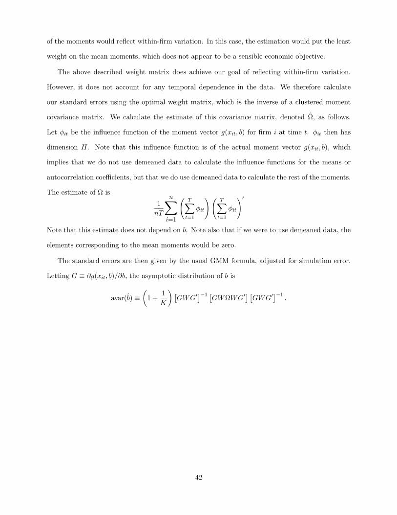
of the moments would reflect within-firm variation. In this case, the estimation would put the least

weight on the mean moments, which does not appear to be a sensible economic objective.

The above described weight matrix does achieve our goal of reflecting within-firm variation.

However, it does not account for any temporal dependence in the data. We therefore calculate

our standard errors using the optimal weight matrix, which is the inverse of a clustered moment

covariance matrix. We calculate the estimate of this covariance matrix, denoted Ω, as follows.

Let φit be the influence function of the moment vector g(xit, b) for firm i at time t. φit then has

dimension H. Note that this influence function is of the actual moment vector g(xit, b), which

implies that we do not use demeaned data to calculate the influence functions for the means or

autocorrelation coefficients, but that we do use demeaned data to calculate the rest of the moments.

The estimate of Ω is

1

nT

n∑i=1

(T∑t=1

φit

)(T∑t=1

φit

)′Note that this estimate does not depend on b. Note also that if we were to use demeaned data, the

elements corresponding to the mean moments would be zero.

The standard errors are then given by the usual GMM formula, adjusted for simulation error.

Letting G ≡ ∂g(xit, b)/∂b, the asymptotic distribution of b is

avar(b) ≡(

1 +1

K

)[GWG′

]−1 [GWΩWG′

] [GWG′

]−1.

42

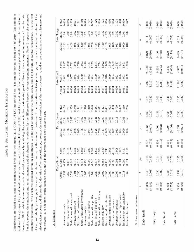
Tab

le2:

Sim

ulated

MomentsEst

imation

Calc

ula

tions

are

base

don

asa

mple

of

nonfinanci

al

firm

sfr

om

the

annual

2011

CO

MP

UST

AT

indust

rial

file

s.T

he

sam

ple

per

iod

isfr

om

1987

to2010.

The

sam

ple

is

split

into

four

gro

ups:

larg

eand

small

firm

sin

the

firs

tpart

of

the

sam

ple

(thro

ugh

2003),

and

larg

eand

small

firm

sin

the

seco

nd

part

of

the

sam

ple

.T

he

esti

mati

on

is

done

wit

hSM

M,

whic

hdet

erm

ines

stru

ctura

lm

odel

para

met

ers

by

matc

hin

gth

em

om

ents

from

asi

mula

ted

panel

of

firm

sto

the

corr

esp

ondin

gm

om

ents

from

the

data

.

Panel

Are

port

sth

esi

mula

ted

and

act

ual

mom

ents

and

the

clust

ered

t-st

ati

stic

sfo

rth

ediff

eren

ces

bet

wee

nth

eco

rres

pondin

gm

om

ents

.P

anel

Bre

port

sth

ees

tim

ate

d

stru

ctura

lpara

met

ers,

wit

hcl

ust

ered

standard

erro

rsin

pare

nth

eses

.λ

isth

eco

stof

adju

stin

gth

eca

pit

al

stock

,andδ

isth

era

teof

capit

al

dep

reci

ati

on.µ

isth

edri

ft

of

the

pro

fita

bilit

ypro

cess

,ρz

isit

sse

rial

corr

elati

on,

andσz

isth

est

andard

dev

iati

on

of

the

innov

ati

on

toth

ispro

cess

.ρψ

andσψ

are

the

seri

al

corr

elati

on

of

the

mis

valu

ati

on

pro

cess

and

the

standard

dev

iati

on

of

its

innov

ati

on.ρzψ

gov

erns

the

seri

al

corr

elati

on

of

the

two

pro

cess

es.νi

andνr

are

pen

alt

ies

on

equit

yis

suance

and

repurc

hase

s.a1

isth

efixed

equit

yis

suance

cost

,andφ

isth

epro

port

ional

deb

tis

suance

cost

.

A.

Mom

ents

Earl

y/Sm

all

Earl

y/L

arg

eL

ate

/Sm

all

Late

/L

arg

eA

ctual

Model

t-st

at

Act

ual

Model

t-st

at

Act

ual

Model

t-st

at

Act

ual

Model

t-st

at

Aver

age

net

cash

-0.1

37

-0.1

78

2.2

68

-0.2

38

-0.2

34

-0.1

58

-0.0

35

-0.0

61

1.8

47

-0.1

93

-0.1

94

0.0

38

Std

.dev

.of

net

cash

0.1

50

0.1

70

-4.1

65

0.1

36

0.1

26

1.7

61

0.1

44

0.1

48

-0.9

90

0.1

31

0.1

05

3.8

86

Ser

ial

corr

elati

on

net

cash

0.5

32

0.9

49

-3.4

07

0.4

13

0.9

47

-4.2

58

0.6

36

0.9

57

-2.7

31

0.4

68

0.8

44

-3.2

25

Aver

age

inves

tmen

t0.0

91

0.0

79

1.3

56

0.0

88

0.0

80

0.8

80

0.0

70

0.0

65

0.9

86

0.0

66

0.0

67

-0.6

21

Std

.dev

.of

inves

tmen

t0.0

55

0.0

15

4.5

52

0.0

45

0.0

12

3.3

41

0.0

43

0.0

24

2.7

10

0.0

34

0.0

27

1.2

41

Ser

ial

corr

elati

on

inves

tmen

t0.6

11

0.5

74

1.0

29

0.7

06

0.5

07

1.7

47

0.6

63

0.6

60

0.0

23

0.6

19

0.6

35

-0.1

10

Aver

age

pro

fits

0.1

65

0.1

56

0.7

02

0.1

91

0.1

81

1.3

16

0.1

42

0.1

32

1.4

18

0.1

80

0.1

74

0.8

15

Std

.dev

.of

pro

fits

0.0

89

0.0

90

-0.2

33

0.0

74

0.0

63

1.2

10

0.0

85

0.0

83

0.4

31

0.0

65

0.0

71

-1.7

07

Ser

ial

corr

elati

on

pro

fits

0.7

63

0.5

43

1.3

89

0.8

07

0.4

28

2.0

28

0.8

83

0.6

04

1.2

53

0.7

66

0.6

40

0.7

97

Std

.dev

.of

Tobin

’sq

0.5

29

0.5

77

-1.6

93

0.5

26

0.5

41

-0.3

81

0.5

38

0.5

90

-1.8

04

0.4

34

0.4

73

-1.1

26

Ser

ial

corr

elati

on

Tobin

’sq

0.6

69

0.0

93

6.9

38

0.7

38

0.1

85

4.5

71

0.6

42

0.3

91

2.7

74

0.7

45

0.6

14

1.0

05

Ret

urn

std.

dev

.0.5

07

0.3

85

2.5

50

0.4

17

0.2

99

6.4

21

0.5

47

0.4

92

1.9

22

0.4

40

0.3

82

1.1

28

Ret

urn

seri

al

corr

elati

on

-0.0

55

-0.4

15

2.2

41

-0.0

69

-0.3

82

8.4

01

-0.0

43

-0.3

15

6.6

53

-0.1

03

-0.1

74

1.0

55

Aver

age

equit

yis

suance

0.0

09

0.0

09

-0.0

96

0.0

07

0.0

06

1.9

23

0.0

10

0.0

09

0.5

99

0.0

05

0.0

03

1.6

56

Std

.dev

.of

issu

ance

0.0

33

0.0

35

-1.1

80

0.0

27

0.0

26

1.3

03

0.0

33

0.0

34

-0.5

82

0.0

23

0.0

20

1.8

66

Aver

age

repurc

hase

s0.0

06

0.0

04

0.9

08

0.0

12

0.0

11

0.7

59

0.0

06

0.0

21

-12.5

37

0.0

21

0.0

32

-3.1

23

Std

.dev

.of

repurc

hase

s0.0

30

0.0

04

3.8

68

0.0

34

0.0

12

3.4

92

0.0

37

0.0

25

3.5

04

0.0

40

0.0

37

1.4

90

Issu

ance

-ret

urn

sensi

tivit

y0.0

11

0.0

00

3.4

51

0.0

09

0.0

01

1.3

19

0.0

11

0.0

03

1.6

01

0.0

09

0.0

04

0.9

59

Issu

ance

Inci

den

ce0.0

62

0.0

74

-1.1

19

0.0

55

0.0

50

1.2

55

0.0

66

0.0

69

-0.2

23

0.0

40

0.0

32

1.6

72

B.

Para

met

eres

tim

ate

s

λδ

ρψ

σψ

µρz

σz

νi

νr

ρzψ

a0

φ

Earl

ySm

all

15.3

58

0.0

46

0.0

13

0.2

47

-1.0

64

0.4

69

0.4

73

3.7

92

29.4

30

0.0

79

0.0

14

0.0

28

(8.1

10)

(0.0

01)

(0.4

30)

(0.0

71)

(0.0

47)

(0.0

25)

(0.0

22)

(1.5

19)

(39.9

24)

(0.5

70)

(0.0

06)

(0.0

30)

Earl

yL

arg

e19.1

51

0.0

50

0.1

14

0.2

09

-1.0

04

0.4

33

0.3

06

4.0

15

9.2

24

0.1

46

0.0

15

0.0

28

(2.9

60)

(0.0

02)

(0.4

63)

(0.0

75)

(0.0

43)

(0.0

16)

(0.0

45)

(1.7

00)

(8.5

85)

(0.7

48)

(0.0

02)

(0.0

33)

Late

Sm

all

6.3

04

0.0

85

0.0

04

0.2

91

-0.7

98

0.6

35

0.4

41

6.5

98

6.4

96

0.3

72

0.0

18

0.0

29

(2.5

55)

(0.0

18)

(0.1

70)

(0.0

33)

(0.1

66)

(0.0

61)

(0.0

63)

(1.4

38)

(2.0

04)

(0.1

73)

(0.0

57)

(0.0

29)

Late

Larg

e3.8

38

0.1

32

0.3

55

0.2

97

-0.6

37

0.6

50

0.2

95

11.2

80

4.9

27

0.4

99

0.0

14

0.0

00

(0.8

20)

(0.0

10)

(0.7

61)

(0.1

56)

(0.0

71)

(0.0

29)

(0.0

32)

(3.5

22)

(0.9

61)

(0.7

97)

(0.0

08)

(0.0

02)

43

Tab

le3:

Sim

ulated

MomentsEst

imation:Pricing

KernelModel

Calc

ula

tions

are

base

don

asa

mple

of

nonfinanci

al

firm

sfr

om

the

annual

2011

CO

MP

UST

AT

indust

rial

file

s.T

he

sam

ple

per

iod

isfr

om

1987

to2010.

The

sam

ple

is

split

into

four

gro

ups:

larg

eand

small

firm

sin

the

firs

tpart

of

the

sam

ple

(thro

ugh

2003),

and

larg

eand

small

firm

sin

the

seco

nd

part

of

the

sam

ple

.T

he

esti

mati

on

is

done

wit

hSM

M,

whic

hdet

erm

ines

stru

ctura

lm

odel

para

met

ers

by

matc

hin

gth

em

om

ents

from

asi

mula

ted

panel

of

firm

sto

the

corr

esp

ondin

gm

om

ents

from

the

data

.

Panel

Are

port

sth

esi

mula

ted

and

act

ual

mom

ents

and

the

clust

ered

t-st

ati

stic

sfo

rth

ediff

eren

ces

bet

wee

nth

eco

rres

pondin

gm

om

ents

.P

anel

Bre

port

sth

ees

tim

ate

d

stru

ctura

lpara

met

ers,

wit

hcl

ust

ered

standard

erro

rsin

pare

nth

eses

.λ

isth

eco

stof

adju

stin

gth

eca

pit

al

stock

,andδ

isth

era

teof

capit

al

dep

reci

ati

on.µ

isth

edri

ft

of

the

pro

fita

bilit

ypro

cess

,ρz

isit

sse

rial

corr

elati

on,

andσz

isth

est

andard

dev

iati

on

of

the

innov

ati

on

toth

ispro

cess

.ρψ

andσψ

are

the

seri

al

corr

elati

on

of

the

mis

valu

ati

on

pro

cess

and

the

standard

dev

iati

on

of

its

innov

ati

on.ρzψ

gov

erns

the

seri

al

corr

elati

on

of

the

two

pro

cess

es.νi

andνr

are

pen

alt

ies

on

equit

yis

suance

and

repurc

hase

s.a1

isth

efixed

equit

yis

suance

cost

,andφ

isth

epro

port

ional

deb

tis

suance

cost

.

A.

Mom

ents

Earl

y/Sm

all

Earl

y/L

arg

eL

ate

/Sm

all

Late

/L

arg

eA

ctual

Model

t-st

at

Act

ual

Model

t-st

at

Act

ual

Model

t-st

at

Act

ual

Model

t-st

at

Aver

age

net

cash

-0.1

37

-0.1

44

0.1

70

-0.2

38

-0.2

36

-0.1

33

-0.0

35

-0.0

34

-0.0

95

-0.1

93

-0.1

94

0.0

84

Std

.dev

.of

net

cash

0.1

50

0.1

53

-0.2

28

0.1

36

0.1

30

1.4

67

0.1

44

0.1

46

-0.3

28

0.1

31

0.1

35

-0.5

15

Ser

ial

corr

elati

on

net

cash

0.5

32

0.9

36

-3.2

85

0.4

13

0.9

24

-4.1

17

0.6

36

0.9

47

-2.5

00

0.4

68

0.8

35

-3.2

52

Aver

age

inves

tmen

t0.0

91

0.0

88

0.3

40

0.0

88

0.0

83

0.6

81

0.0

70

0.0

73

-0.7

10

0.0

66

0.0

66

0.1

39

Std

.dev

.of

inves

tmen

t0.0

55

0.0

22

4.0

17

0.0

45

0.0

13

3.2

70

0.0

43

0.0

21

3.6

93

0.0

34

0.0

17

2.9

73

Ser

ial

corr

elati

on

inves

tmen

t0.6

11

0.5

35

0.6

47

0.7

06

0.2

99

5.2

59

0.6

63

0.5

98

0.7

16

0.6

19

0.6

31

-0.0

85

Aver

age

pro

fits

0.1

65

0.1

55

0.5

79

0.1

91

0.1

87

0.2

84

0.1

42

0.1

36

0.5

17

0.1

80

0.1

79

0.3

87

Std

.dev

.of

pro

fits

0.0

89

0.0

92

-0.2

97

0.0

74

0.0

59

1.7

96

0.0

85

0.0

77

1.3

43

0.0

65

0.0

66

-0.2

26

Ser

ial

corr

elati

on

pro

fits

0.7

63

0.4

04

2.6

58

0.8

07

0.4

28

2.0

99

0.8

83

0.6

48

1.6

85

0.7

66

0.7

22

0.2

84

Std

.dev

.of

Tobin

’sq

0.5

29

0.5

02

0.3

99

0.5

26

0.4

93

0.9

42

0.5

38

0.5

24

0.9

08

0.4

34

0.4

14

0.9

59

Ser

ial

corr

elati

on

Tobin

’sq

0.6

69

0.4

11

1.5

78

0.7

38

0.4

40

2.3

19

0.6

42

0.4

92

1.5

31

0.7

45

0.6

39

1.3

09

Ret

urn

std.

dev

.0.5

07

0.5

03

0.1

17

0.4

17

0.4

03

1.2

37

0.5

47

0.5

36

1.9

06

0.4

40

0.4

40

0.0

07

Ret

urn

seri

al

corr

elati

on

-0.0

55

-0.2

48

2.2

23

-0.0

69

-0.3

44

3.9

26

-0.0

43

-0.3

33

5.0

84

-0.1

03

-0.2

53

2.3

75

Aver

age

equit

yis

suance

0.0

09

0.0

06

1.1

58

0.0

07

0.0

06

0.4

17

0.0

10

0.0

06

1.8

28

0.0

05

0.0

06

-1.1

51

Std

.dev

.of

issu

ance

0.0

33

0.0

28

1.0

36

0.0

27

0.0

26

0.5

30

0.0

33

0.0

26

2.7

77

0.0

23

0.0

25

-1.5

70

Aver

age

repurc

hase

s0.0

06

0.0

04

0.5

38

0.0

12

0.0

12

0.0

30

0.0

06

0.0

12

-2.9

91

0.0

21

0.0

28

-1.8

96

Std

.dev

.of

repurc

hase

s0.0

30

0.0

06

3.7

96

0.0

34

0.0

32

0.6

55

0.0

37

0.0

37

-0.1

98

0.0

40

0.0

33

1.0

85

Issu

ance

-ret

urn

sensi

tivit

y0.0

11

0.0

03

1.2

54

0.0

09

0.0

01

1.1

30

0.0

11

0.0

01

2.6

78

0.0

09

0.0

03

1.0

76

Issu

ance

Inci

den

ce0.0

62

0.0

50

0.7

69

0.0

55

0.0

55

-0.0

71

0.0

66

0.0

55

0.9

47

0.0

40

0.0

53

-1.0

81

-0.1

3594531

0.0

0000000

-0.0

0991879

-0.1

2486226

2.9

6005669

0.0

0000000

2.2

6352211

-0.0

0379203

0.0

0024355

0.2

2005898

-0.7

7294241

0.7

6563236

B.

Para

met

eres

tim

ate

s

λδ

ρψ

σψ

µρz

σz

νi

νr

ρzψ

a0

φ

Earl

ySm

all

10.0

27

0.0

56

0.4

33

0.3

66

-1.1

37

0.4

36

0.4

91

12.8

01

29.5

33

0.0

03

0.0

29

0.0

40

(1.3

59)

(0.0

09)

(0.1

24)

(0.0

29)

(0.0

96)

(0.0

35)

(0.0

37)

(4.3

55)

(2.2

00)

(0.1

54)

(0.0

03)

(0.0

61)

Earl

yL

arg

e19.4

40

0.0

50

0.2

16

0.2

85

-0.9

69

0.4

38

0.2

78

15.0

56

0.6

43

0.1

47

0.0

30

0.0

06

(0.6

00)

(0.0

06)

(0.1

67)

(0.0

36)

(0.1

62)

(0.0

91)

(0.0

48)

(3.9

38)

(1.1

20)

(0.2

23)

(0.0

04)

(0.6

09)

Late

Sm

all

12.7

46

0.0

65

0.2

11

0.3

60

-0.6

86

0.6

78

0.3

88

20.3

10

1.1

76

0.0

15

0.0

30

0.0

25

(2.0

76)

(0.0

12)

(0.1

26)

(0.0

18)

(0.0

80)

(0.0

27)

(0.0

36)

(3.3

14)

(2.0

11)

(0.0

57)

(0.0

08)

(0.3

62)

Late

Larg

e11.1

58

0.0

98

0.3

24

0.3

32

-0.4

71

0.7

36

0.2

44

9.2

27

5.2

81

0.3

00

0.0

19

0.0

07

(2.4

03)

(0.0

05)

(0.1

92)

(0.0

26)

(0.0

89)

(0.0

46)

(0.0

32)

(1.4

06)

(1.1

47)

(0.2

55)

(0.2

06)

(0.0

16)

44

Table 4: Parameter Estimates for Industry Estimations

Calculations are based on a sample of nonfinancial firms from the annual 2011 COMPUSTAT industrial files. The sample period is

from 1987 to 2010. The sample is split into eight industry groups. SIC13 is oil and gas extraction; SIC20 is food products; SIC28

is chemicals and allied products; SIC35 is machinery and computer equipment; SIC26 is electronic and electrical equipment; SIC38 is

measuring instruments; SIC50 is wholesale trade; and SIC73 is business services. The estimation is done with SMM, which determines

structural model parameters by matching the moments from a simulated panel of firms to the corresponding moments from the data.

The estimation is done for each industry separately. This table reports the estimated structural parameters, with clustered standard

errors in parentheses. λ is the cost of adjusting the capital stock, and δ is the rate of capital depreciation. µ is the drift of the

profitability process, ρz is its serial correlation, and σz is the standard deviation of the innovation to this process. ρψ and σψ are the

serial correlation of the misvaluation process and the standard deviation of its innovation. ρzψ governs the serial correlation of the two

processes. νi and νr are penalties on equity issuance and repurchases. a1 is the fixed equity issuance cost, and φ is the proportional

debt issuance cost. The bottom row of the table presents average R&D for each industry.

SIC13 SIC 20 SIC 28 SIC 35 SIC 36 SIC 38 SIC 50 SIC 73λ 2.267 18.634 2.072 10.435 3.708 19.947 8.350 11.757

(0.713) (15.310) (2.144) (8.748) (1.975) (9.515) (17.169) (6.447)

δ 0.168 0.057 0.146 0.062 0.073 0.045 0.051 0.076(0.004) (0.017) (0.052) (0.013) (0.017) (0.011) (0.046) (0.024)

ρψ 0.291 0.000 0.854 0.172 0.152 0.006 0.012 0.199(1.025) (0.432) (0.110) (0.806) (0.767) (1.245) (0.724) (0.801)

σψ 0.345 0.113 0.431 0.323 0.313 0.130 0.132 0.330(0.114) (0.114) (0.111) (0.192) (0.135) (0.158) (0.179) (0.107)

µ -0.724 -0.704 -1.193 -0.808 -1.126 -1.329 -0.889 -0.716(0.042) (0.212) (0.552) (0.191) (0.215) (0.288) (0.316) (0.201)

ρz 0.506 0.612 0.381 0.632 0.485 0.336 0.630 0.632(0.032) (0.105) (0.231) (0.059) (0.112) (0.151) (0.126) (0.110)

σz 0.384 0.294 0.493 0.500 0.500 0.449 0.430 0.456(0.064) (0.138) (0.168) (0.174) (0.126) (0.107) (0.166) (0.081)

νi 4.127 4.215 20.962 6.666 20.216 6.905 6.160 6.937(3.260) (3.228) (8.946) (4.070) (33.227) (5.818) (7.072) (2.054)

νr 39.055 3.506 30.982 5.754 1.569 0.723 5.642 4.454(58.041) (7.478) (22.729) (4.283) (0.882) (2.556) (8.110) (1.501)

ρzψ 0.086 0.493 0.490 0.238 0.169 0.414 0.496 0.316(1.591) (0.517) (0.201) (0.666) (0.699) (1.071) (0.531) (0.721)

a0 0.012 0.014 0.024 0.024 0.024 0.025 0.015 0.024(0.031) (0.154) (0.224) (0.011) (0.033) (0.020) (0.012) (0.006)

φ 0.029 0.012 0.029 0.034 0.034 0.023 0.021 0.034(0.453) (0.068) (0.035) (0.123) (0.084) (0.083) (0.441) (0.195)

Average R&D 0.001 0.003 0.064 0.060 0.071 0.027 0.001 0.062

45

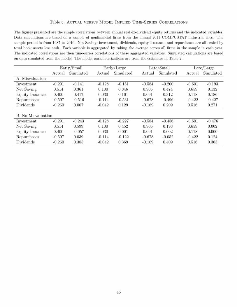
Table 5: Actual versus Model Implied Time-Series Correlations

The figures presented are the simple correlations between annual real ex-dividend equity returns and the indicated variables.

Data calculations are based on a sample of nonfinancial firms from the annual 2011 COMPUSTAT industrial files. The

sample period is from 1987 to 2010. Net Saving, investment, dividends, equity Issuance, and repurchases are all scaled by

total book assets less cash. Each variable is aggregated by taking the average across all firms in the sample in each year.

The indicated correlations are then time-series correlations of these aggregated variables. Simulated calculations are based

on data simulated from the model. The model parameterizations are from the estimates in Table 2.

Early/Small Early/Large Late/Small Late/LargeActual Simulated Actual Simulated Actual Simulated Actual Simulated

A. Misvaluation

Investment -0.291 -0.141 -0.128 -0.151 -0.584 -0.200 -0.601 -0.193Net Saving 0.514 0.361 0.100 0.346 0.905 0.474 0.659 0.132Equity Issuance 0.400 0.417 0.030 0.161 0.091 0.312 0.118 0.186Repurchases -0.597 -0.516 -0.114 -0.531 -0.678 -0.496 -0.422 -0.427Dividends -0.260 0.067 -0.042 0.129 -0.169 0.209 0.516 0.271

B. No Misvaluation

Investment -0.291 -0.243 -0.128 -0.227 -0.584 -0.456 -0.601 -0.476Net Saving 0.514 0.599 0.100 0.452 0.905 0.193 0.659 0.002Equity Issuance 0.400 -0.057 0.030 0.001 0.091 0.002 0.118 0.000Repurchases -0.597 0.039 -0.114 -0.122 -0.678 -0.052 -0.422 0.124Dividends -0.260 0.385 -0.042 0.369 -0.169 0.409 0.516 0.363

46

Figure 1: Time Series Patterns: Small Firms

A.

Repurchases Dividends Equity Issuance Return

Equi

ty Is

suan

ce, R

epur

chas

es, D

ivid

ends

−0.005

0

0.005

0.010

0.015

0.020

0.025

0.030

Return

−0.4

−0.2

0

0.2

0.4

0.6

1988 1990 1992 1994 1996 1998 2000 2002 2004 2006 2008 2010

B.

Return Saving Debt Issuance

Savi

ng, D

ebt I

ssua

nce

−0.06

−0.04

−0.02

0

0.02

0.04

0.06

Return

−0.4

−0.2

0

0.2

0.4

0.6

1988 1990 1992 1994 1996 1998 2000 2002 2004 2006 2008 2010

C.

Repurchases Dividends Equity Issuance Return

Equi

ty Is

suan

ce, R

epur

chas

es, D

ivid

ends

−0.005

0

0.005

0.010

0.015

0.020

0.025

0.030

Return

−0.4

−0.2

0

0.2

0.4

0.6

1988 1990 1992 1994 1996 1998 2000 2002 2004 2006 2008 2010

Calculations are based on a sample of nonfinancial firms from the annual 2011 COMPUSTAT industrial files. The sample

period is from 1987 to 2010. Each series is the year-by-year asset-weighted average of a particular variable. Small firms are

those whose assets are below the median for a particular year in the sample. Investment, dividends, equity Issuance, saving,

debt Issuance, and repurchases are all scaled by total book assets. Saving is the change in the stock of cash. Return is the

real annual ex-dividend equity return.

47

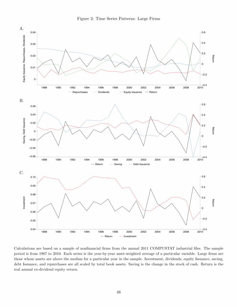
Figure 2: Time Series Patterns: Large Firms

A.

Repurchases Dividends Equity Issuance Return

Equi

ty Is

suan

ce, R

epur

chas

es, D

ivid

ends

0

0.01

0.02

0.03

0.04

Return

−0.4

−0.2

0

0.2

0.4

0.6

1988 1990 1992 1994 1996 1998 2000 2002 2004 2006 2008 2010

B.

Return Saving Debt Issuance

Savi

ng, D

ebt I

ssua

nce

−0.06

−0.04

−0.02

0

0.02

0.04

0.06

Return

−0.4

−0.2

0

0.2

0.4

0.6

1988 1990 1992 1994 1996 1998 2000 2002 2004 2006 2008 2010

C.

Return Investment

Inve

stm

ent

0.04

0.05

0.06

0.07

0.08

0.09

0.10

Return

−0.4

−0.2

0

0.2

0.4

0.6

1988 1990 1992 1994 1996 1998 2000 2002 2004 2006 2008 2010

Calculations are based on a sample of nonfinancial firms from the annual 2011 COMPUSTAT industrial files. The sample

period is from 1987 to 2010. Each series is the year-by-year asset-weighted average of a particular variable. Large firms are

those whose assets are above the median for a particular year in the sample. Investment, dividends, equity Issuance, saving,

debt Issuance, and repurchases are all scaled by total book assets. Saving is the change in the stock of cash. Return is the

real annual ex-dividend equity return.

48

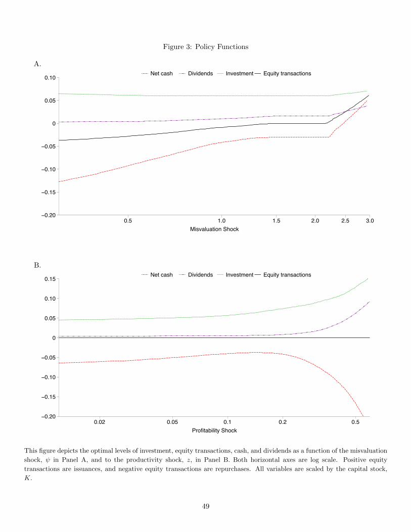
Figure 3: Policy Functions

A.

Net cash Dividends Investment Equity transactions

−0.20

−0.15

−0.10

−0.05

0

0.05

0.10

Misvaluation Shock0.5 1.0 1.5 2.0 2.5 3.0

B.

Net cash Dividends Investment Equity transactions

−0.20

−0.15

−0.10

−0.05

0

0.05

0.10

0.15

Profitability Shock0.02 0.05 0.1 0.2 0.5

This figure depicts the optimal levels of investment, equity transactions, cash, and dividends as a function of the misvaluation

shock, ψ in Panel A, and to the productivity shock, z, in Panel B. Both horizontal axes are log scale. Positive equity

transactions are issuances, and negative equity transactions are repurchases. All variables are scaled by the capital stock,

K.

49

Figure 4: Matching Moments by Industry

A. B.

13

20

28

3536

38

50

73

Actu

al N

et C

ash

−0.3

−0.2

−0.1

0

0.1

Simulated Net Cash−0.2 −0.1 0 0.1

13

202835

3638

50

73

Actu

al In

vest

men

t0

0.05

0.10

0.15

0.20

Simulated Investment0 0.05 0.10 0.15 0.20

C. D.

13

20

28

3536

3850 73Ac

tual

Equ

ity Is

suan

ce

0

0.005

0.010

0.015

0.020

0.025

Simulated Equity Issuance0 0.005 0.010 0.015 0.020 0.025

13

20

28 35

36

38 50

73

Actu

al R

epur

chas

es

0

0.005

0.010

0.015

0.020

0.025

0.030

Simulated Repurchases0 0.005 0.010 0.015 0.020 0.025 0.030

Calculations are based on a sample of nonfinancial firms from the annual 2011 COMPUSTAT industrial files. The sample period is

from 1987 to 2010. The sample is split into eight industry groups. SIC13 is oil and gas extraction; SIC20 is food products; SIC28

is chemicals and allied products; SIC35 is machinery and computer equipment; SIC26 is electronic and electrical equipment; SIC38 is

measuring instruments; SIC50 is wholesale trade; and SIC73 is business services. The estimation is done with SMM, which determines

structural model parameters by matching the moments from a simulated panel of firms to the corresponding moments from the data.

This figure plots data moments versus simulated moments for four of the “mean” moments.

50

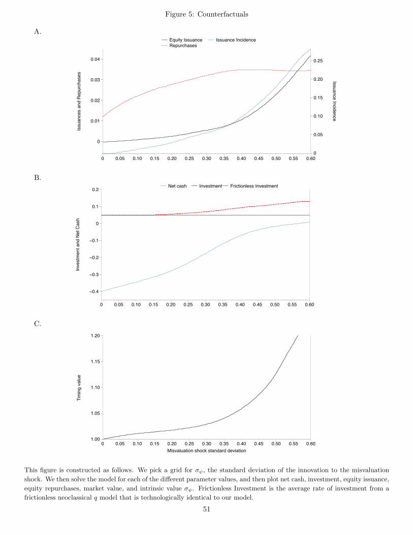
Figure 5: Counterfactuals

A.Equity IssuanceRepurchases

Issuance Incidence

Issu

ance

s an

d R

epur

chas

es

0

0.01

0.02

0.03

0.04

Issuance Incidence

0

0.05

0.10

0.15

0.20

0.25

0 0.05 0.10 0.15 0.20 0.25 0.30 0.35 0.40 0.45 0.50 0.55 0.60

B.Net cash Investment Frictionless Investment

Inve

stm

ent a

nd N

et C

ash

−0.4

−0.3

−0.2

−0.1

0

0.1

0.2

Net C

ash

0 0.05 0.10 0.15 0.20 0.25 0.30 0.35 0.40 0.45 0.50 0.55 0.60

C.

Tim

ing

valu

e

1.00

1.05

1.10

1.15

1.20

lal

Misvaluation shock standard deviation0 0.05 0.10 0.15 0.20 0.25 0.30 0.35 0.40 0.45 0.50 0.55 0.60

This figure is constructed as follows. We pick a grid for σψ, the standard deviation of the innovation to the misvaluation

shock. We then solve the model for each of the different parameter values, and then plot net cash, investment, equity issuance,

equity repurchases, market value, and intrinsic value σψ. Frictionless Investment is the average rate of investment from a

frictionless neoclassical q model that is technologically identical to our model.

51

Figure 6: Impulse Response Functions

A.Profit shock Misvaluation shock

Net

Cas

h

−0.03

−0.02

−0.01

0

0.01

0.02

Time1 2 3 4 5

B.Profit shock Misvaluation shock

Inve

stm

ent

−0.03

−0.02

−0.01

0

0.01

0.02

Time1 2 3 4 5

C.Profit shock Misvaluation shock

Equi

ty is

suan

ce

−0.03

−0.02

−0.01

0

0.01

0.02

Time1 2 3 4 5

D.Profit shock Misvaluation shock

Rep

urch

ases

−0.03

−0.02

−0.01

0

0.01

0.02

Time1 2 3 4 5

This figure depicts the responses of various variables to a one standard deviation innovation to each of the misvaluation and

profit shock processes.

52