equity premium prediction state of the economy
TRANSCRIPT
Copyright belongs to the author. Short sections of the text, not exceeding three paragraphs, can be used
provided proper acknowledgement is given.
The Rimini Centre for Economic Analysis (RCEA) was established in March 2007. RCEA is a private,
nonprofit organization dedicated to independent research in Applied and Theoretical Economics and related
fields. RCEA organizes seminars and workshops, sponsors a general interest journal, the Review of Economic
Analysis (REA), and organizes a biennial conference, the Rimini Conference in Economics and Finance
(RCEF). Scientific work contributed by the RCEA Scholars is published in the RCEA Working Paper series.
The views expressed in this paper are those of the authors. No responsibility for them should be attributed to
the Rimini Centre for Economic Analysis.
Rimini Centre for Economic Analysis
www.rcea.org
May/2020 Working Paper 20-16
rcea.org/RePEc/pdf/wp20-16.pdf
EQUITY PREMIUM PREDICTION
AND THE STATE OF THE ECONOMY
Ilias Tsiakas
University of Guelph, Canada
RCEA
Jiahan Li
GMO LLC
Haibin Zhang
University of Guelph, Canada

Equity Premium Predictionand the State of the Economy∗
Ilias Tsiakas Jiahan Li Haibin Zhang
University of Guelph GMO LLC University of Guelph
[email protected] [email protected] [email protected]
May 2020
Abstract
We detect cyclical variation in the predictive information of economic fundamentals,
which can be used to substantially improve and simplify out-of-sample equity premium pre-
diction. Economic fundamentals based on stock-specific information (notably the dividend
yield) deliver better predictions in expansions. Economic fundamentals based on aggregate
information (notably the short rate) deliver better predictions in recessions. Accordingly, a
simple forecast combination of one predictor that generates cyclical forecasts and one predic-
tor that generates countercyclical forecasts can deliver statistically significant and economi-
cally valuable equity premium predictions in both expansions and recessions. A prominent
two-predictor forecast combination that performs well is the dividend yield and the short
rate. Strategies designed for ex-ante timing of the business cycle can provide additional
economic gains in equity premium prediction.
Keywords: Equity Premium; Out-of-Sample Prediction; Economic Fundamentals; Business
Cycle; Financial Cycle; Diversification.
JEL Classification: G11; G14; G17.∗This paper is forthcoming in the Journal of Empirical Finance. Acknowledgements: The authors
are grateful for useful comments to Nikola Gradojevic, Gikas Hardouvelis, Angelo Melino and seminarparticipants at the University of Toronto, the 2016 RCEF Conference in Waterloo, and the 2017 EFMAConference in Athens. This research was supported by the Social Sciences and Humanities Research Councilof Canada (grant number 430418) and was conducted while Ilias Tsiakas was visiting the University ofToronto. The views expressed herein are those of the authors alone and do not necessarily reflect thoseof GMO or its personnel. Corresponding author : Ilias Tsiakas, Department of Economics and Finance,Lang School of Business and Economics, University of Guelph, Guelph, Ontario N1G 2W1, Canada. Tel:519-824-4120 ext. 53054. Fax: 519-763-8497. Email: [email protected].

1 Introduction
Does the state of the economy matter for equity premium prediction? According to a recent
study by Kacperczyk, Van Nieuwerburgh, and Veldkamp (2016), the state of the economy
changes the way investors process information. In recessions, aggregate risk is significantly
higher and, consequently, investors care more about aggregate shocks. In expansions, ag-
gregate risk is significantly lower and, consequently, investors care more about idiosyncratic
shocks. This framework implies that the predictive information of economic fundamentals
may be linked to the observed state of the business cycle.
In this paper, we find that the state of the economy does matter for equity premium pre-
diction. The empirical evidence indicates that certain economic fundamentals (notably the
dividend yield) generate equity premium forecasts that perform well in good times, whereas
other economic fundamentals (notably the short rate) generate forecasts that perform well
in bad times. Motivated by this finding, we propose a simple way to predict the equity pre-
mium out of sample: form an equally weighted forecast combination of one predictor that
generates cyclical forecasts and one predictor that generates countercyclical forecasts. For
example, we can form a simple forecast combination of the dividend yield and the short rate.
We show that this approach has solid theoretical foundations and achieves two desirable
properties: diversification, which implies that the combined forecast performs better than
any individual forecast; and insurance, which implies that the combined forecast performs
well in every state of the world.
Our main analysis focuses on the dividend yield and the short rate but we also consider
other two-predictor forecast combinations. The dividend yield and the short rate are per-
haps the two most prominent predictors for stock returns in the literature. They are also
theoretically motivated by the present value framework of Campbell and Shiller (1988). The
dividend yield is a measure of idiosyncratic information because it is based on stock-specific
dividends and prices. Therefore, consistent with the Kacperczyk, Van Nieuwerburgh, and
Veldkamp (2016) framework, it is expected to be more informative in expansions. In con-
trast, the short rate is a measure of aggregate information because it is an economy-wide
variable that affects the future returns and cash flows of all firms. As a result, it is expected
to be more informative in recessions. It is no surprise, therefore, that our analysis provides
strong empirical support for the cyclical predictive ability of the dividend yield and the coun-
tercyclical predictive ability of the short rate. This, in turn, motivates the equally weighted
forecast combination of the two predictors as a simple, yet powerful, out-of-sample approach
for equity premium prediction.
Our empirical findings are based on a standard predictive framework. We employ monthly
1

equity premium returns and the 14 monthly economic fundamentals of Welch and Goyal
(2008) for a sample period ranging from January 1927 to December 2017. The Welch and
Goyal (2008) data set focuses on the excess return to the S&P 500 index. All predictors are
US variables used to predict the S&P 500 index excess returns. We estimate simple pre-
dictive regressions and impose the economic constraints of Campbell and Thompson (2008)
on the sign of the regression coeffi cients and return forecasts. The constraints impose eco-
nomic theory on the predictive regressions and almost universally improve performance. The
analysis is performed purely out-of-sample in order to inform real-time investment decisions.
Our main empirical finding is that the equally weighted forecast combination of the
dividend yield and the short rate delivers a statistically significant monthly out-of-sample
R2 of 1.5%. This is considerably higher than the value of: (1) the R2 of the best individual
model; and (2) the standard forecast combination based on all 14 predictors. Therefore, the
simple forecast combination achieves diversification. More importantly, the equally weighted
forecast combination of the dividend yield and the short rate delivers good performance in
both expansions (R2 = 1.6%) and recessions (R2 = 1.3%). Therefore, the simple forecast
combination also achieves insurance, a property that is not achieved by any of the individual
models. Finally, it also delivers high economic value in the context of a dynamic mean-
variance strategy: the certainty equivalent return is about 2.1% per year over and above the
historical mean benchmark for the full sample, 1.8% per year in expansions, and 3.6% per
year in recessions.
The forecast combination we propose has two features that make it simple and attractive:
equal weights and using only two predictors. Both of these features are based on solid
foundations. The choice of equal weights on the two predictors is not only a simple choice
that works well, but it is also an optimal choice. This is because, for the data set we employ,
the optimal weights that maximize the diversification gains of this forecast combination are
close to equal weights.
Using only two predictors is also a good choice because: (1) the forecasts generated by
the two predictors are negatively correlated with each other; and (2) the forecasts generated
by one of the two predictors are highly positively correlated with the forecasts of all other
predictors that perform well in the same state of the world. For example, the performance of
the dividend yield is highly correlated with that of the earnings-price ratio. Therefore, adding
the latter in a forecast combination adds very little to the performance of the combination.
Similarly, the performance of the short rate is highly correlated to that of the long rate or
the term spread. Again, adding any of the latter two predictors in a forecast combination
does not improve much the performance of the combination.
It is important to emphasize that a combination of the dividend yield and the short rate is
2

not uniquely powerful. There are several two-predictor combinations that perform well. For
example, we could replace the dividend yield by the earnings-price ratio, or the short rate by
the term spread, and the resulting two-predictor combination would perform similarly well.
Two-predictor forecast combinations based on one cyclical forecast and one countercyclical
forecast have the potential to perform well. We propose the specific combination because
the dividend yield and the short rate are popular predictors in the literature, they are
theoretically motivated by the present value framework of Campbell and Shiller (1988),
one captures systematic risk while the other one idiosyncratic risk, and they perform well
in different states of the economy. Therefore, this two-predictor combination is a natural
choice to be the main focus of our analysis.
In this context, we formally evaluate the ex-ante performance of several two-predictor
forecast combinations. We take the point of view of an econometrician who, at a given
point in time, must decide which model to use for forecasting based on the out-of-sample
performance of each model up to that point. We find that the dividend yield and short
rate combination is consistently one of the top combinations, and often the top combina-
tion, at every point in time during the out-of-sample period. Therefore, an econometrician
who considers the ex-ante evidence up to a given date is likely to use this combination for
forecasting.
Our findings provide an explanation for why standard forecast combinations of all 14
predictors typically work well. Since the contribution of Rapach, Strauss, and Zhou (2010),
forecast combinations of all available predictors have become popular primarily because
they are simple and work well. By naively combining the forecasts of all predictors, the
standard approach includes some forecasts that work well in expansions, some that work
well in recessions and some that work well in neither. We show that by excluding from the
combination the forecasts that work well in neither state of the economy, in addition to those
that add no further diversification gains, we can form simpler and yet superior combinations.
We also consider two formal rules for ex-ante timing of the business cycle. The first rule
is based on the Markov-switching dynamic factor model of Chauvet (1998), which produces a
probability that the economy is in expansion or recession every month. We establish turning
point dates by converting the probability into a dummy variable for forecasting which state
the economy is in at a given point in time. The second rule is based on the Hodrick and
Prescott (1980) filter for estimating the output gap. Following Colacito, Riddiough and
Sarno (2019), the sign of the output gap can be used to forecast the future state of the
economy.
We find that, overall, the ex-ante timing strategies perform very well, especially in re-
cessions. The best ex-ante timing strategy is based on whether the output gap is increasing
3

or decreasing at a given point in time. For example, whereas the simple mean combination
provides a certainty equivalent return of about 2%, for the timing strategies it rises to about
3%. To conclude, we find that the ex-ante timing strategies provide a more sophisticated
and better performing alternative to the simple mean combination.
In addition, we assess the cyclical variation of equity premium predictions around another
cycle: the financial cycle. Following Claessens, Kose and Terrones (2012), we use data
on aggregate credit from the Bank for International Settlements to identify the phases of
the financial cycle: the recovery phase (from trough to peak) called the “upturn”, and
the contraction phase (from peak to trough) called the “downturn”. We find that our
results remain qualitatively the same for the business cycle, the financial cycle and the
combination of the two cycles. The equally weighted forecast combination of the dividend
yield and the short rate has essentially the same performance in either of the two cycles
and delivers a positive and significant out-of-sample R2 in both expansions/upturns and
recessions/downturns. Therefore, our main finding is robust to determining the state of the
economy around either the business cycle or the financial cycle.
Finally, we report international evidence for four additional countries: Canada, UK,
Germany and Japan. For these countries the sample period is substantially shorter than for
the US. We find that for three of the countries (Canada, UK and Japan) our main result
holds: the dividend yield is a powerful predictor in expansions, whereas the short rate is a
powerful predictor in recessions. However, the performance of the simple mean combination
is not as strong as in the US. This is because the dividend yield and the short rate perform
very well in one state of the economy but very poorly in other state of the economy. For
this reason, the ex-post and ex-ante timing strategies perform better than the simple mean
combination in the international context.
Our analysis adds to the well-known theoretical and empirical finding that stock return
predictability concentrates in bad times. The intuition behind this finding is primarily based
on countercyclical risk premiums (e.g., Campbell and Cochrane, 1999; Menzly, Santos and
Veronesi, 2004; and Bekaert, Engstrom and Xing, 2009) and, more recently, on countercycli-
cal investor disagreement about the state of the economy (Cujean and Hasler, 2017). The
empirical evidence on this finding is reported in Henkel, Martin and Nardari (2011), who
use a regime-switching vector autoregression framework to show that standard predictors of
the equity premium are effective primarily in recessions. Our analysis extends the Henkel,
Martin and Nardari (2011) findings by focusing on out-of-sample prediction to show that
there are both cyclical and countercyclical forecasts so that a simple combination of the two
delivers better predictions in good and bad times.
Overall, this paper contributes to a long line of research on the out-of-sample predictabil-
4

ity of the equity premium. Rapach and Zhou (2013) review this research and propose the
following groupings for the forecasting models that deliver statistically and economically
significant out-of-sample gains: (1) economically motivated model restrictions (e.g., Camp-
bell and Thompson, 2008; Ferreira and Santa-Clara, 2011; Pettenuzzo, Timmermann and
Valkanov, 2014; Li and Tsiakas, 2017); (2) forecast combination (e.g., Rapach, Strauss and
Zhou, 2010); (3) diffusion indices (e.g., Ludvigson and Ng, 2007; Kelly and Pruitt, 2013;
Neely, Rapach, Tu and Zhou, 2014); and (4) regime shifts and structural breaks (e.g., Paye
and Timmermann, 2006; Guidolin and Timmermann, 2007; Lettau and Van Nieuwerburgh,
2008; Henkel, Martin and Nardari, 2011; Dangl and Halling, 2012). In this setting, the
contribution of our paper is best described as a refinement of a forecast combination with
economically motivated model restrictions.
The remainder of the paper is organized as follows. In the next section, we examine the
theoretical foundations of our analysis. The data on economic fundamentals are described
in Section 3. In Section 4, we discuss the predictive framework and the empirical results. In
Section 5, we provide an empirical analysis of the ex-ante selection of several two-predictor
forecast combinations. The dynamic mean-variance strategy for evaluating the portfolio
performance of equity premium predictability is described in Section 6. We evaluate the
performance of strategies timing the business cycle in Section 7. In Section 8, we evaluate
the performance of the models around financial cycles and in Section 9 we report some
international evidence. Finally, we conclude in Section 10.
2 Theoretical foundations
In this section, we discuss the theoretical foundations of our predictive approach by answering
three questions. First, why is the dividend yield and the short rate the main focus of our
analysis? Second, why does the state of the business cycle matter? Finally, third, why does
the simple forecast combination provide superior results in equity premium prediction?
2.1 Motivating the choice of predictors
We use the present value framework of Campbell and Shiller (1988) to motivate the choice of
the dividend yield (or equivalently the dividend-price ratio) and the short rate as predictors
of the future equity premium. We also show that similar arguments can be used to motivate
replacing the dividend-price ratio by the earnings-price ratio or the short rate by the long
rate.
Campbell and Shiller (1988) show that the following difference equation holds approxi-
5

mately:
dpt = −k + ρdpt+1 + rt+1 −∆dt+1, (1)
where dpt is the log dividend-price ratio, k is a known constant, ρ < 1 is also a known con-
stant, rt+1 is the one-period stock return including dividends, and ∆dt+1 is the log dividend
growth rate.
Iterating forward and taking the time t expectation of both sides, we arrive at the fol-
lowing equation:
dpt = − k
1− ρ + Et
∞∑j=0
ρj (rt+j+1 −∆dt+j+1) . (2)
This equation relates the dividend-price ratio (or equivalently the dividend yield) with future
returns, and hence motivates the dividend yield as a predictor of the equity premium.2
Equation (2) can be re-written in terms of future excess returns as follows:
dpt − rf,t = − k
1− ρ + Et
∞∑j=0
ρj(ret+j+1 −∆dt+j+1
)+ Et
∞∑j=1
ρjrf,t+j, (3)
where ret+1 = rt+1 − rf,t, and rf,t is the one-period risk-free rate. This equation motivatesthe short rate as a relevant predictor of future excess returns.
Equation (3) can have two additional forms that are relevant for our analysis. Specifically,
we can replace the short rate by the long rate by further assuming the pure expectations
hypothesis of the term structure: yn,t = 1n
n−1∑j=0
Et (rf,t+j), where yn,t is the yield of an n-period
bond. Then, Equation (3) becomes:
dpt − nyn,t = − k
1− ρ + Et
∞∑j=0
ρj(ret+j+1 −∆dt+j+1
)+ Et
∞∑j=n
ρjrf,t+j. (4)
This equation suggests that the long rate can also be a relevant predictor of future excess
returns.
Finally, we return to Equation (1) and add the log earnings growth rate ∆et+1 to both
sides. Solving forward, we can then show that the following equation holds for the log
earnings-price ratio, det:
det − rf,t = − k
1− ρ + Et
∞∑j=0
ρj(ret+j+1 −∆et+j+1 − (1− ρ) det+j+1
)+ Et
∞∑j=1
ρjrf,t+j. (5)
This equation shows that det contains similar information to dpt for predicting future excess
2See also Cochrane (2008, 2011) on the prominent role of the dividend yield in stock return predictability.
6
returns.
In summary, Equation (2) shows that the current dividend-price ratio (or equivalently
the dividend yield) is related to future returns. Given our focus on the equity premium,
which is defined as an excess return, Equation (3) suggests that the current short rate is also
related to future excess returns. Therefore, the dividend yield and the short rate are directly
motivated by the present value framework of Campbell and Shiller (1988). In addition,
Equations (4) and (5) further suggest that we can replace the dividend-price ratio by the
earnings-price ratio or the short rate by the long rate.3 Consequently, there are alternative
two-predictor combinations motivated by this framework and the choice of which one to use
remains an empirical issue to be examined later.
2.2 Why does the business cycle matter?
The state of the business cycle is an important variable in predicting stock returns. It
is abundantly clear in the asset pricing literature that during recessions we observe three
effects: (1) returns are unexpectedly low, (2) returns are more volatile, and (3) the price of
risk is higher, partly driven by higher risk aversion (e.g., Fama and French, 1989). This is
also true in our sample since the equity premium during recessions is on average negative
(−5.7% annually) and its volatility is high (30% annually).
More importantly, Kacperczyk, Van Nieuwerburgh, and Veldkamp (2016) show that the
state of the economy changes the way investors process information. They propose a the-
oretical model, which describes how the optimal attention allocation of investors depends
on the business cycle. They also provide empirical evidence, which strongly indicates that
aggregate risk is significantly higher in recessions. As a result, skilled investors (e.g., mutual
funds) care more about aggregate shocks in recessions, which is revealed by a higher covari-
ance between portfolio weights and aggregate shocks. In other words, skilled investors have
better timing ability in recessions.
The empirical evidence of Kacperczyk, Van Nieuwerburgh, and Veldkamp (2016) also
shows that idiosyncratic risk is essentially the same in expansions and recessions. In expan-
sions, when aggregate risk is lower, skilled investors care more about idiosyncratic shocks,
which is revealed by a higher covariance between portfolio weights and idiosyncratic shocks.
In other words, skilled investors have better picking ability in expansions.
The intuition behind these empirical findings is straightforward. Information is most
valuable when uncertainty is higher. In recessions, when aggregate risk is higher, skilled
investors will allocate their attention towards aggregate risk. Learning more about aggregate
3The derivation of Equations (1)-(5) is straightforward using the approach of Campbell and Shiller(1998). Further details on these derivations can be found in Maio (2013).
7

risk is the most effi cient way to resolve uncertainty and reduce portfolio risk. In expansions,
when aggregate risk is low, they will allocate their attention towards idiosyncratic risk.
Overall, this framework links information choices (aggregate vs. idiosyncratic) to the
observed state of the business cycle and motivates our findings in the following way: interest
rates (such as the short rate) are economy-wide variables that reflect aggregate risk and
hence they are more informative in recessions; in contrast, variables such as the dividend
yield, the dividend-price ratio and the earnings-price ratio reflect idiosyncratic risk, since
they are based on stock-specific dividends, earnings and prices, and hence they are more
informative in expansions.
2.3 Diversification gains of combined forecasts
It is well known that a portfolio investing in two negatively correlated assets exhibits diver-
sification gains: the return variance of the portfolio is lower than the average return variance
of the two assets. In this section, we show that this diversification result has a direct ana-
logue in forecasting. A forecast combination of two negatively correlated forecasts can be
thought of as a portfolio of forecasts that also delivers diversification gains: the variance of
the forecast error of the combination is lower than the average variance of the forecast error
of the individual models.
To better understand this claim, consider the simple linear predictive regression:
ret+1 = α + βxt + εt+1, (6)
where ret+1 = rt+1 − rf,t is the equity premium at time t + 1, rt+1 is the total return on the
S&P 500 Index at time t+ 1, rf,t is the Treasury bill rate, xt is a predictor at time t, α and
β are estimated with ordinary least squares (OLS), and εt+1 is a normal error term.
We form forecasts r̂et+1 = α̂ + β̂xt, where α̂ and β̂ are the OLS estimates. The forecast
error ε̂t+1 = ret+1 − r̂et+1 is unbiased with E[εt] = 0 and V ar[εt] = σ2. The predictive
performance of the model, captured by the mean squared error (MSE) of the forecasts, is
directly linked to the variance of the forecast error:
MSE = E[(ret+1 − r̂et+1
)2]= E
[ε2t+1
]= σ2. (7)
2.3.1 The case of equal weights
Consider two models that generate forecasts r̂1,t+1 and r̂2,t+1. We form an equally weighted
combined forecast: r̂c,t+1 = 12r̂1,t+1 + 1
2r̂2,t+1. Suppose that the correlation ρ12 between the
forecast errors of the two models is less than one. Then, it is straightforward to show that
8

the diversification condition holds:
σc <1
2σ1 +
1
2σ2. (8)
Equation (8) states that the MSE of the combined forecasts (σc) is lower than the weighted
average of the individual MSEs (σ1, σ2). This condition is directly analogous to standard
portfolio diversification.4
For forecasting purposes, it is of greater interest if ρ12 is “low enough”so that the “strong”
diversification condition holds:
σc < min(σ1, σ2). (9)
If this condition holds, then the forecast combination will produce superior predictive ability
compared to any of the two models individually. To describe the conditions under which the
strong diversification holds, we turn to the more general case of optimal weights.
2.3.2 The general case
Instead of assuming equal weights, we can generalize this framework by choosing the weights
w1 and w2 that minimize the objective function:
σ2c = w21σ21 + w22σ
22 + 2w1w2σ1σ2ρ12. (10)
Solving for the optimal weights gives:
w∗1 =σ22 − σ1σ2ρ12
σ21 + σ22 − 2σ1σ2ρ12, (11)
w∗2 =σ21 − σ1σ2ρ12
σ21 + σ22 − 2σ1σ2ρ12. (12)
Inserting the optimal weights into the objective function (10), we get the MSE associated
with the optimal weights:
σ2∗c =σ21σ
22 (1− ρ212)
σ21 + σ22 − 2σ1σ2ρ12. (13)
In this framework, Timmermann (2006) shows that the following results hold: if σ1 =
σ2 = σ and ρ12 < 1, then equal weights are optimal and the strong diversification condi-
tion holds. Moreover, we attain maximum diversification gains, that is the largest reduction
4To see this consider ρ12 = 1. Then, σ2c =
14σ
21+
14σ
22+
12σ1σ2 =
14 (σ1 + σ2)
2. Hence, σc = 12σ1+
12σ2 and
there is no diversification benefit from combining forecasts. If instead ρ12 < 1, the diversification conditionholds.
9

in σ2∗c /σ for a given change in ρ12.5 These results are crucially important for our empiri-
cal exercise. By carefully selecting two individual forecasts with similar performance (i.e.,
σ1 ≈ σ2), where each performs better in a different state of the world (i.e., ρ12 < 1), then
the equally weighted combination can deliver maximum diversification gains and superior
predictive performance. In the following sections, our empirical analysis shows that this is
indeed the case for the equally weighted forecast combination of two predictors such as the
dividend yield and the short rate.
3 Data on economic fundamentals
We use a set of monthly economic fundamentals for predicting the monthly equity premium
for the period of January 1927 to December 2017.6 All data are taken from Amit Goyal’s
website. These are the same data used in Welch and Goyal (2008), Campbell and Thompson
(2008), Dangl and Halling (2012), Neely et al. (2014), and Pettenuzzo, Timmermann, and
Valkanov (2014) extended to 2017.
Most of our results are reported for the full sample and the two subsamples of expan-
sions and recessions. We measure recessions using the definition of the National Bureau of
Economic Research (NBER) business cycle dating committee. The start of a recession is the
period following the peak of economic activity and its end is the trough.
The equity premium is the continuously compounded return on the S&P 500 Index
including dividends obtained from CRSP minus the Treasury bill rate (defined below). For
the full sample, the equity premium in annualized terms exhibits a mean return of 7.9%,
volatility of 19%, and a Sharpe ratio of 0.42. For expansions, the annualized Sharpe ratio of
the equity premium rises to 0.71 and for recessions it falls to −0.20. Recessions correspond
to about 18% of the full sample and are known ex post.
The economic fundamentals include the following 14 monthly predictors:
1. Dividend yield (dy) is the difference between the log of dividends and the log of lagged
prices.
2. Dividend-price ratio (dpr) is the difference between the log of dividends and the log of
current prices.
5Note that in the extreme case where σ1 = σ2 and ρ12 = −1, σ2∗c = 0, which implies perfect forecastingability for the equally weighted combination.
6Throughout the analysis, we fix both the frequency and the horizon to be monthly for three reasons:(i) monthly predictability is notoriously diffi cult to achieve; (ii) given that recessions are less than 20% ofthe sample, monthly data provides the most recession observations; and (iii) long horizons complicate theanalysis because for a long horizon some months in the horizon may be in recession and some in expansion.
10

3. Earnings-price ratio (epr) is the difference between the log of earnings and the log of
prices.
4. Dividend payout ratio (dpayr) is the difference between the log of dividends and the
log of earnings.
5. Book-to-market ratio (bm) is the ratio of book value to market value for the Dow Jones
Industrial Average.
6. Net equity expansion (ntis) is the ratio of twelve-month moving sums of net issues by
NYSE-listed stocks divided by the total market capitalization of NYSE stocks.
7. Stock variance (svar) is the sum of squared daily returns on the S&P 500.
8. Treasury bill rate (tbl) is the 3-month rate.
9. Long-term yield (lty) on government bonds.
10. Term spread (tms) is the difference between lty and tbl.
11. Long-term rate of return (ltr) for government bonds.
12. Default yield spread (dfy) is the difference between BAA-rated and AAA-rated corpo-
rate bond yields.
13. Default return spread (dfr) is the difference between the return on long-term corporate
bonds and the return on long-term government bonds.
14. Inflation (infl). Note that inflation information is released in the following month.
Therefore, we lag inflation by an additional month in the predictive regressions.
The cross-correlations between the predictors range from−0.466 to 0.993, with an average
value of 0.095.
4 Models for predicting the equity premium
4.1 Our predictive framework
We generate forecasts for the equity premium by OLS estimation of the predictive regression
in Equation (6). Our analysis is based on conditioning on a single predictor every time
we estimate the predictive regression. Hence, we report results from 14 regressions each
conditioning on one of the Welch and Goyal (2008) predictors. We then form an equally
11
weighted combination of just the dy and tbl forecasts, which is the focal point of our analysis.
We refer to this combined forecast as the “simple mean combination.”
Following Campbell and Thompson (2008), we also impose two constraints motivated by
economic theory. First, we constrain the equity premium forecast to be positive in every time
period. We do so by replacing negative forecasts with zero. Campbell and Thompson (2008)
argue that a reasonable investor would not have used a model to forecast a negative equity
premium. The positive forecast constraint is also implemented by Pettenuzzo, Timmermann,
and Valkanov (2014).
Second, we constrain the sign of the slope coeffi cients to be consistent with economic
theory. Campbell and Thompson (2008, p. 1516) explain that “[a] regression estimated over
a short sample period can easily generate perverse results, such as a negative coeffi cient
when theory suggests that the coeffi cient should be positive... In practice, an investor would
not use a perverse coeffi cient but would likely conclude that the coeffi cient is zero, in effect
imposing prior knowledge on the output of the regression.”We implement this constraint by
setting a value of zero for a coeffi cient that does not have the theoretically motivated sign
of Campbell and Thompson (2008). To be more specific, the slope constraint is positive for
all predictors except for dpayr, ntis, tbl, lty, and infl. As we report later, these economic
constraints considerably improve the performance of the models.
4.2 Standard forecast combinations
A natural alternative to our predictive framework is to form standard forecast combinations
using all 14 forecasts generated by the predictive regressions that condition on one predictor
at a time. Following Rapach, Strauss, and Zhou (2010), we compute the equally weighted
average of all forecasts at each point in time. We refer to this as the “standard mean
combination”to be distinguished from the “simple mean combination”described above.7
4.3 The benchmark
The benchmark against which we compare all models is the historical mean for the equity
premium. This is the prevalent benchmark in the literature and corresponds to the case of
β = 0 in Equation (6). In other words, the historical mean benchmark reflects the view that
the expected equity premium is constant and hence it is not predictable when conditioning
on economic fundamentals.7We have also considered other combinations of the 14 forecasts, such as the combination based on the
most recent MSE of each model. However, the performance of the additional standard combinations is verysimilar to the standard mean combination. For this reason, these results remain unreported but availableupon request.
12

4.4 Out-of-sample analysis
All empirical models are evaluated out-of-sample relative to the historical mean benchmark.
We generate out-of-sample forecasts with rolling predictive regressions using a 20-year esti-
mation window such that the first forecast is for January 1947 and the last for December
2017. We adopt a rolling window approach to be consistent with Welch and Goyal (2008)
and the ensuing literature.
The main statistical criterion for evaluating the out-of-sample predictive ability of the
models is the Campbell and Thompson (2008) and Welch and Goyal (2008) R2oos statistic.
The R2oos compares the unconditional one-month ahead forecasts ret+1|t of the historical mean
benchmark to the conditional forecasts r̂et+1|t of the alternative model, and is defined as
follows:
R2oos = 1−MSE
(r̂et+1|t
)MSE
(ret+1|t
) = 1−
T−1∑t=1
(ret+1 − r̂et+1|t
)2T−1∑t=1
(ret+1 − ret+1|t
)2 . (14)
A positive R2oos implies that the alternative model outperforms the benchmark by means of
lower MSE.
We assess the statistical significance of the R2oos statistic by applying the Clark and West
(2006, 2007) testing procedure. This is a test of the null hypothesis of equal predictive
ability between the benchmark and the alternative model. The Clark and West (2006, 2007)
procedure accounts for the fact that, under the null, the MSE of the benchmark is expected
to be lower. This is because the alternative models estimate a parameter vector that, under
the null, is not helpful in prediction thus introducing noise into the forecasting process. Clark
and West (2006, 2007) adjust the MSE as follows:
MSEadj =1
T − 1
T−1∑t=1
(ret+1−r̂et+1|t)2 −1
T − 1
T−1∑t=1
(ret+1|t − r̂et+1|t)2. (15)
Then, we define:
t̂estt+1 = (ret+1 − ret+1|t)2 − [(ret+1 − r̂et+1|t)2 − (ret+1|t − r̂et+1|t)2], (16)
and regress t̂estt+1 on a constant, using the t-statistic for a zero coeffi cient. Even though the
asymptotic distribution of this test is non-standard (e.g., McCracken, 2007), Clark and West
(2006, 2007) show that standard normal critical values provide a good approximation and,
therefore, recommend to reject the null of equal predictive ability if the statistic is greater
than +1.282 (for a one-sided 0.10 test) or +1.645 (for a one-sided 0.05 test) or +2.326 (for
13

a one-sided 0.01 test).
4.5 Empirical results
4.5.1 Individual predictors
We begin our analysis by focusing on the out-of-sample performance of the 14 individual
predictors. This allows us to identify which predictors perform well, whether economic
constraints improve performance, and whether the performance of the predictors depends
on the state of the economy. We report results for the full sample as well as NBER-dated
expansions and recessions. The results for expansions and recessions are based on estimating
the models each month over the full forecasting period and then separating the forecasting
errors ex post across the two subsamples as in Neely et al. (2014).
Table 1 reports the R2oos. In the case of no economic constraints, the only two predictors
that exhibit a positive and statistically significant R2oos are the dividend yield (dy) with an
R2oos of 0.53% and the dividend-price ratio (dpr) with an R2oos of 0.26%.8 The other 12
predictors display a negative R2oos. For example, the short rate (tbl) exhibits an R2oos of
−1.64%. In the absence of constraints, therefore, only dy and dpr beat the historical mean,
while all other predictors appear to be devoid of any predictive information over and above
the benchmark.
This finding changes considerably with the imposition of the two economic constraints as
they universally improve performance: the R2oos rises for 13 of the 14 predictors, the single
exception being the dividend payout ratio (dpayr). Under the constraints, seven predictors
exhibit a positive and significant R2oos. Notably, the R2oos of the dividend yield rises to
1.07%, and is significant at 1%, whereas the R2oos of the short rate rises to a positive value
(0.46%) and is significant at 5%. In short, therefore, economic constraints are instrumental
in revealing the predictive information of economic fundamentals. For this reason, the rest
of our analysis imposes the constraints.
The most important finding in Table 1 is that certain economic fundamentals perform well
in expansions, whereas others perform well in recessions. Indeed, none of the 14 predictors
performs well in both states of the economy. In expansions, predictors associated with stock
dividends and earnings, such as the dividend yield and the earnings-price ratio, display a
positive and statistically significant R2oos. In recessions, predictors associated with interest
rates, such as the short rate, the long rate and the term spread, also display a positive and
statistically significant R2oos. Therefore, predictors that capture stock-specific information
8These two predictors (dy and dpr) are virtually the same by definition and their correlation exceeds99%. Our discussion will therefore focus on dy as it is more popular in the literature than dpr.
14

on dividends and earnings have good predictive power in good times. In contrast, predictors
that capture aggregate economy-wide information on interest rates have good predictive
power in bad times. This finding is consistent with the theory and empirical evidence of
Kacperczyk, Van Nieuwerburgh, and Veldkamp (2016) on the cyclical variation of investor
attention allocation.
4.5.2 The simple mean combination
Next we turn to the main model of our analysis: the equally weighted forecast combination of
the dividend yield and the short rate. As mentioned earlier, we refer to this as the “simple
mean combination.” Indeed, this is the simplest possible combination we can form: two
predictors with equal weights, where one predictor performs well in expansions and one in
recessions. In what follows, we will show that this is a powerful forecast combination that is
hard to beat.
To quantify the diversification gains of the simple mean combination consider the results
of Table 2. The dividend yield alone delivers an R2oos of 1.07% and the short rate alone an
R2oos of 0.46%. An equally weighted combination of the two delivers an R2oos of 1.54%, which
is considerably higher than the R2oos of the better model. This implies that the MSE of the
simple mean combination is much lower than the lowest MSE of the two predictors. Hence
the simple mean combination satisfies the strong diversification condition of Equation (9).
Moreover, the simple mean combination provides insurance since it delivers good per-
formance in both expansions (R2oos = 1.63%) and recessions (R2oos = 1.28%), where in both
cases the R2oos is statistically significant. In conclusion, therefore, the simple mean combi-
nation of the forecasts generated by the dividend yield and the short rate delivers strong
diversification gains and insurance.
The simple mean combination has two features that make it simple and attractive: equal
weights and using only two predictors. We will now explain why both of these features make
sense. In addition to being a simple choice, setting equal weights also turns out to be an
optimal choice: when computing the optimal diversification weights using Equations (11) and
(12), the result is a weight of 54% on the dividend yield and 46% on the short rate. Therefore,
from the point of view of diversification, using equal weights is practically as good as it gets.
It also means that the simple mean combination achieves maximum diversification gains for
two reasons: (1) σ1 ≈ σ2, i.e., the similar MSE values of the two models; and (2) ρ12 < 1
since one set of forecasts is cyclical and one countercyclical. Consequently, the simple mean
combination achieves the maximum diversification gains defined by Timmermann (2006) as
the largest reduction in σ2∗c /σ for a given change in ρ12.
Using only two predictors is also a good choice because: (1) the two predictors are
15

negatively correlated with each other; and (2) each predictor is highly positively correlated
with the other predictors that perform well in the same state of the world. In other words,
the performance of dy is highly correlated with that of dpr and epr. Therefore, adding any
of the latter two forecasts does not add much to the performance of the initial combination.
Similarly, the performance of the short rate (tbl) is highly correlated to that of the long rate
(lty), the term spread (tms), and the long-term return (ltr). Again, adding any of the latter
three forecasts does not improve much the performance of the initial combination.
This finding is illustrated in Table 3, which reports on the performance of more forecast
combinations. The table shows that the performance of the simple mean combination re-
mains almost the same when: (1) we replace dy by dpr or epr, (2) we replace tbl by tms, lty
or ltr ; and (3) we add with equal weights to the dy+tbl combination any one of the following:
dpr, epr, tms, lty or ltr. In all these cases, the results are similar in the sense that all these
models deliver a positive and significant R2oos, which remains positive and significant in both
expansions and recessions.
These results imply that the simple mean combination of dy and tbl is not unique in
delivering a good performance in both states of the economy. We could replace dy by epr,
or tbl by tms, and the resulting two-predictor combination would have similar performance.
Our proposed combination is based on dy and tbl because, as mentioned earlier, these two
are the most popular predictors with solid theoretical foundations. A combination of these
two predictors is hard to improve on. Having said that, we show that one can also combine
say epr with tms and achieve similar diversification and insurance results.9
It is also important to note that the simple mean combination of dy and tbl significantly
outperforms the standard forecast combinations of all 14 predictors. Since Rapach, Strauss,
and Zhou (2010) forecast combinations of all available predictors have become popular,
partly due to their simplicity. We show here that simpler combinations can perform much
better if we carefully select the forecasts to combine in a way that achieves diversification
gains. Indeed, our simple approach not only outperforms the standard combination but
also justifies why the standard combination works: by naively combining all predictors, we
effectively combine some that work well in expansions, some that work well in recessions and
some that work well in neither. Then, by excluding from the combination the predictors
that work well in neither state of the economy, in addition to the ones that offer no further
diversification gains, we can form a simpler, yet superior, combination.
To illustrate these results, Figure 1 plots the out-of-sample performance of selected mod-
9We also report results on typical combinations of idiosyncratic and systematic predictors. As expected,larger groups of idiosyncratic predictors perform well in expansions, whereas larger groups of systematicpredictors perform well in recessions. This further confirms the cyclical performance of the two types ofpredictors.
16

els over time. Following Welch and Goyal (2008), the figure shows the difference of the
cumulative squared error of the null (historical mean) minus the cumulative squared error of
the alternative. The figure shows that the simple mean combination of dy and tbl displays a
consistent upward trend in its out-of-sample performance over time. Hence the good perfor-
mance of this model is not due to a particular subsample but is systematic over a long sample
spanning the full postwar period. The figure also shows that the simple mean combination
outperforms the standard mean forecast combination based on all 14 predictors. Finally, the
simple mean combination strongly outperforms its two individual components, the dividend
yield and the short rate.10
4.5.3 The ex-post timing strategy
Finally, consider the strategy perfectly timing the business cycle using the true recession
dummy. This strategy can only be implemented ex post and hence it is not directly compa-
rable to the out-of-sample strategies discussed above. This strategy, however, is informative
for the following reason. By design, the ex-post timing strategy can perfectly time which
forecasts to use: it uses the dividend yield forecasts in expansions and the short rate forecasts
in recessions. Hence there is no averaging in the two sets of forecasts at a given point in time.
This generates a profound difference between the simple mean combination and the timing
strategy: the former maximizes the diversification gains, whereas the latter maximizes the
insurance gains. Therefore, a comparison of the two strategies informs us of how close the
simple mean combination comes to achieving the maximum insurance gains.
We find that the R2oos of the two strategies is very similar: the ex-post timing strategy
(R2oos = 1.71%) is only marginally better than the simple mean combination (R2oos = 1.54%).
The two strategies have almost identical performance in expansions, while the timing strategy
performs slightly better in recessions. This is to be expected since there is more predictabil-
ity in recessions and so perfectly timing the business cycle delivers better performance in
recessions. However, the main result here is that the simple mean combination, which is
a fully ex-ante strategy, is impressively close to providing the maximum insurance gains in
addition to the maximum diversification gains discussed previously.
10In addition, we have also performed estimation using the adjustment proposed by Kostakis, Magdalinosand Stamatogiannis (2015) for persistent regressors. However, this procedure is not designed for forecastcombinations based on out-of-sample estimation with economic constraints. Instead this procedure can beused for in-sample estimation using individual predictors without economic constraints. Therefore, we donot report these results but they are available upon request.
17
5 Ex-ante selection of two-predictor forecast combina-
tions
The main thesis of this paper is that a two-predictor forecast combination is a simple yet
powerful tool in out-of-sample equity premium prediction. This forecast combination works
well as long as one predictor performs well in expansions and the other one performs well
in recessions. In other words, this forecast combination can be thought of as a portfolio
of one cyclical and one countercyclical forecast so that the forecasts generated by the two
predictors are negatively correlated with each other. Furthermore, the forecasts generated
by each of the two predictors are highly positively correlated with the forecasts of all other
predictors that perform well in the same state of the world. Accordingly, the two-predictor
forecast combination achieves diversification, which implies that the combined forecast per-
forms better than any individual forecast, and insurance, which implies that the combined
forecast performs well in every state of the world.
There are several two-predictor combinations that achieve these results. Our analysis
focuses on the dividend yield and the short rate for the following reasons: these are popular
predictors in the literature, they are theoretically motivated by the present value framework
of Campbell and Shiller (1988), one captures systematic risk while the other one idiosyncratic
risk, and they perform well in different states of the economy. Therefore, this two-predictor
combination is a natural choice to be the focus of our analysis.
Having said that, however, there are other two-predictor combinations that also perform
well. In this section, we provide an empirical analysis that informs the ex-ante selection of
two-predictor forecast combinations. We consider a set of two-predictor combinations, where
the dividend yield (dy) is replaced by the dividend-price ratio (dpr) or the earnings-price ratio
(epr); and the short rate (tbl) is replaced by the term spread (tms) or the long-term yield
(lty) or the long-term rate of return (ltr). This leads to 12 different forecast combinations:
dy+tbl ; dy+tms; dy+lty; dy+ltr ; dpr+tbl ; dpr+tms; dpr+lty; dpr+ltr ; epr+tbl ; epr+tms;
epr+lty; epr+ltr. These are the same two-predictor combinations shown in Table 3.
We assess the ex-ante performance of these models from the point of view of an econo-
metrician who, at a given point in time, must decide which model to use for forecasting
based on the out-of-sample performance of each model up to that point. To do so, we di-
vide the out-of-sample period into different training and forecasting periods. The training
period defines the information set of the econometrician and always begins with the first
out-of-sample forecast in January 1947. The training period is specified to include 20, 30,
40, 50 or 60 years of initial out-of-sample forecasts. The forecasting period begins right
after the end of the training period and ends with the last forecast for December 2017. For
18

example, an econometrician making a decision in January 1967 would have knowledge of the
out-of-sample performance of the first training period ending in December 1966. Therefore,
the econometrician would implement a forecasting period from January 1967 till December
2017.
The findings are reported in Table 4. Panel A reports the R2oos for different training and
forecasting periods, whereas Panel B reports the rank of each model relative to all other
models based on the R2oos. We find that, across all training periods, dy+tbl is ranked second
(i.e., its rank of the average rank across all training periods is 2). It is ranked first for the
last and longest training period of 1947-2006. Across all training periods, the first-ranked
model is dy+ltr. Across all forecasting periods, dy+tbl is again ranked second but now the
first-ranked model is different: dy+lty. Finally, across all training and forecasting periods,
dy+tbl is ranked first. In other words, dy+tbl performs consistently well: it is always in the
top two models, it is ranked first for the longest training period and it is ranked first across
all training and forecasting periods. In short, therefore, there is strong empirical evidence
that dy+tbl is a good choice for a two-predictor forecast combination.
The empirical evidence reported in Table 4 fixes the length of training periods to be a
multiple of 10 years beginning with 20 years of initial out-of-sample evidence. The evidence
might be different for alternative definitions of the training period. A more comprehensive
way of reporting the evidence for all possible training periods is by plotting the out-of-sample
performance of each two-predictor model against dy+tbl. This is illustrated in Figures 2-4.
The figures demonstrate the information (in terms of cumulative out-of-sample performance)
available to an econometrician at all points in time. Then, the econometrician considers this
information at a given point in time in order to choose one the models. The figures confirm
that the dy+tbl combination is not uniquely powerful but it is a combination that is hard
to beat at any point in time. Consistent with Table 4, the figures indicate that models
using the dividend yield perform better than models using the dividend-price ratio or the
earnings-price ratio. In addition, the dividend yield plus short rate combination graphically
appears to be as good as or better than any other forecast combination.
In conclusion, we find that there are several two-predictor combinations that perform well
in out-of-sample equity premium prediction. The dividend yield and short rate combination
is consistently one of the top combinations, and often the top combination, at every point
in time during the out-of-sample period. Therefore, an econometrician who considers the
ex-ante evidence up to a given date is likely to use this combination for forecasting. For the
reasons discussed in this section, the remainder of our analysis focuses on the dividend yield
and short rate combination.
19

6 Predictability and asset allocation
6.1 A mean-variance trading strategy
Following Campbell and Thompson (2008), we assess the economic value of equity premium
predictability using a dynamic asset allocation strategy. The strategy involves monthly
rebalancing of a portfolio that invests in the S&P 500 Index (the risky asset) and the Treasury
bill (the riskless asset). We consider a mean-variance investor with a one-month ahead
horizon, who determines the optimal weights by implementing a maximum expected utility
rule as follows:maxwt
Et [U (rp,t+1)] = rp,t+1|t − γ2σ2p,t+1|t
s.t. rp,t+1|t = wtrt+1|t + (1− wt) rf ,σ2p,t+1|t = w2tσ
2t+1|t,
(17)
where rp,t+1|t is the t+ 1 forecast of the portfolio return conditional on time t information, γ
is the investor’s degree of relative risk aversion, σ2p,t+1|t is the t + 1 forecast of the portfolio
variance made at time t, rt+1|t is the t + 1 forecast of the S&P 500 Index return made at
time t, rf is the risk-free rate of return, and σ2t+1|t is the t + 1 forecast of the variance to
the S&P 500 Index return made at time t. Note that we forecast σ2t+1|t using a five-year
rolling average of the variance of past monthly returns as in Campbell and Thompson (2008).
Following Della Corte, Sarno and Tsiakas (2009), we consider two degrees of relative risk
aversion: γ = 2 and γ = 6.
The solution to the maximum expected utility rule delivers the risky asset weight:
wt =1
γ
rt+1|t − rfσ2t+1|t
. (18)
Consistent with the literature (e.g., Campbell and Thompson, 2008; Neely et al., 2014), we
constrain the weight on the risky asset by imposing wt ∈ [0, 1.5]. In other words, short-selling
is not allowed and leverage is limited to no more than 50%.
We evaluate the performance of portfolios generated by a given set of equity premium
forecasts using the Sharpe ratio (SR), the Economic Performance Measure (EPM ) proposed
by Homm and Pigorsch (2012), and the certainty equivalent return (CER). The Sharpe
ratio is perhaps the most commonly used performance measure and is defined as the average
excess return of a portfolio divided by the standard deviation of the portfolio returns. The
statistical significance of the SR is assessed using the Ledoit and Wolf (2008) bootstrap
two-sided test of whether the SR of the alternative model is different from the benchmark.
The Economic Performance Measure is designed to generalize the Sharpe ratio with
20

respect to non-normal return distributions. Based on the Aumann and Serrano (2008) eco-
nomic index of riskiness, the EPM is defined as follows:
EPM =18rp
3κprp − 4rpχ2p − 6χpσp + 9σ2p/rp, (19)
where rp is the mean portfolio return, σ2p is the portfolio variance over the forecast evaluation
period, χp is the skewness of portfolio returns and κp is the excess kurtosis of portfolio returns.
For normally distributed excess returns, EPM =2r2pσ2p
= 2SR2. For this reason, we report√EPM/2 so that the EPM is on the same scale as the Sharpe ratio.
The certainty equivalent return is defined as:
CER =(rp −
γ
2σ2p
). (20)
The CER can be interpreted as the performance fee a risk-averse investor is willing to pay
for switching from the riskless asset to the risky portfolio. We focus on the difference in
CER (∆CER), which is equal to the CER of the portfolio generated by the forecasts of
the alternative model minus the CER of the portfolio generated by the historical mean
benchmark. ∆CER measures the performance fee a risk-averse investor is willing to pay for
switching from the risky portfolio generated by the benchmark model to the risky portfolio
generated by the alternative model.
To provide a realistic assessment of the profitability of dynamic trading strategies, we
also take into account the effect of transaction costs. Following Marquering and Verbeek
(2004), we compute ∆CER using two values for c, which is the proportional transaction cost
per transaction: c = 50 bps reflecting medium transaction costs, and c = 100 bps reflecting
high transaction costs (see also Balduzzi and Lynch, 1999; Neely, Rapach, Tu and Zhou,
2014).
Finally, we compute the average turnover of each trading strategy, which is defined as
follows:
TO =1
T − 1
T−1∑t=1
(|wt+1 − w−t+1|
), (21)
where T − 1 is the number of trading periods, wt+1 is the weight on the risky asset at time
t+ 1, and w−t+1 = wt1+rt+11+rp,t+1
is the weight on the risky asset right before rebalancing at time
t+ 1. This turnover measure represents the average monthly trading volume. We report the
average relative turnover, which is the ratio of the average turnover of the alternative model
divided by the average turnover of the benchmark model.
21

6.2 Portfolio performance
We assess the performance of dynamically rebalanced portfolios generated by the monthly
forecasts of the predictive models. Table 5 reports the empirical findings for two degrees
of relative risk aversion, γ = 2 (Panel A) and γ = 6 (Panel B). Our discussion focuses on
the case of γ = 6, which is the standard case considered in the literature. The results for
γ = 2 are similar. The first finding to note is that the historical mean benchmark delivers a
CER = 5.34% per year relative to riskless investing. The CER rises to 6.76% in expansions
but falls to −3.08% in recessions. Clearly, using the historical mean is a poor predictor of
the equity premium during recessions.
Similar to the statistical findings, our main result here is that the simple mean combina-
tion of the dividend yield and the short rate performs well: better than the historical mean
benchmark, better than the two individual predictors, and better than the standard forecast
combination of all 14 predictors. The ∆CER of the simple mean combination relative to
the benchmark is 2.10% per year. More importantly, the ∆CER remains positive for both
expansions (1.84%) and recessions (3.63%). Net of transaction costs, it still retains a pos-
itive ∆CER of 1.93% per year for medium transaction costs and 1.75% per year for high
transaction costs. Moreover, the annualized SR is 0.64, which is significantly higher than the
0.46 of the benchmark strategy according to the Ledoit and Wolf (2008) bootstrap two-sided
test. The Economic Performance Measure provides similar values and the same ranking as
the Sharpe ratio.
Overall, our evidence shows that, in the context of a dynamic mean-variance strategy, a
simple forecast combination of the dividend yield and the short rate has high economic value
in predicting the equity premium. The economic gains of this approach can be summarized
into a performance fee of approximately 2.1% per year overall, 1.8% per year in expansions,
3.6% per year in recessions, together with a statistically significant increase in the SR from
0.46 to 0.64.
Finally, the ex-post timing strategy using the true recession dummy performs even better
by generating a performance fee of about 3% per year and a Sharpe ratio of 0.74. This is
further evidence that there is high economic value in timing recessions when predictability
is high.11
11It is interesting to note that for lower risk aversion (γ = 2), the performance of the simple meancombination is slightly lower than for higher risk aversion (γ = 6). This is driven by the fact that the lowerthe risk aversion the higher the weight on the risky asset. For higher weight on the risky asset, and giventhat this asset is procyclical, the performance of the historical mean in expansions improves. Similarly,given that the predictive ability of the short rate is countercyclical, the performance of the short rate inrecessions also improves. The net effect of lower risk aversion is slightly lower performance for the simplemean combination. In contrast, the ex-post timing strategy performs well for both levels of risk aversion.
22

6.3 Comparing statistical and economic gains
In this section, we relate the R2 of the models to the SR of the strategies. Following Campbell
and Thompson (2008, p. 1525), “the correct way to judge the magnitude of R2 is to compare
it with the squared Sharpe ratio”since the proportional increase in the expected return is
approximately equal to the ratio of R2oosSR2
, where SR is the unconditional SR of the risky
asset.12
For example, recall that the equally weighted forecast combination of dy and tbl deliv-
ers an R2oos of 1.54%. Over the same forecasting period (1947-2017), the risky asset has
a squared monthly SR of 0.15602 = 0.0243. Then, the proportional increase in the ex-
pected return is 0.0154/0.0243 = 0.6337. In other words, the simple mean combination
will increase the average monthly portfolio return by a factor of 63.37%. Campbell and
Thompson (2008) show that this corresponds to an actual increase in the expected return
of(1γ
)(R2oos1−R2oos
)(1 + SR2) = 0.27% per month or 3.20% per year (for γ = 6). In conclu-
sion, modest predictive ability for the equity premium can plausibly generate large economic
gains.
7 Timing the business cycle
The phase of the business cycle can only be known ex post and hence cannot be used to
inform ex-ante prediction. In fact, the business cycle peak and trough dates are determined
by the NBER’s business cycle dating committee with a substantial lag, often more than
a year later. For this reason, instead of using the actual NBER dates, we now turn to
implementing two distinct formal rules for ex-ante timing of the business cycle.
7.1 Smooth recession probabilities
The first rule is based on the Markov-switching dynamic factor model (DFMS) of Chau-
vet (1998), which produces a probability that the economy is in expansion or a recession
every month. The Chauvet (1998) DFMS model uses information from the four coincident
economic variables highlighted by the NBER in establishing turning point dates: (1) non-
farm payroll employment, (2) industrial production, (3) real manufacturing and trade sales,
and (4) real personal income excluding transfer payments. This information is used by the
12Specifically, when moving from the unconditional forecast of the expected return to a conditional fore-
cast, the proportional increase in the expected return is(
R2oos
1−R2oos
)(1+SR2
SR2
), which is approximately equal
to R2oos
SR2 , when R2oos and SR2 are both small.
23

model to generate the smoothed recession probabilities, which are obtained from the FRED
database of the Federal Reserve Bank of St. Louis.
Our approach for ex-ante timing of the business cycle is as follows. Following Chauvet
and Piger (2008), we identify the first month of a recession as the first month for which the
smooth recession probability rises above 50%. Similarly, an expansion begins on the first
month for which the probability falls below 50%. This formal rule defines our forecasted
recession dummy.13 Chauvet and Piger (2008) find that this approach is very accurate and
identifies peaks and troughs much sooner than the NBER. More importantly, it does not
produce any “false positives,”which are turning points that were established in real time but
did not correspond to an actual NBER turning point date. The first available probability
in the sample is for June 1967, which is used to forecast the business cycle for the following
month.14
7.2 Output Gap
The second rule for timing the business cycle is based on the Hodrick and Prescott (HP)
(1980, 1997) filter. The HP filter is perhaps the most popular way for estimating the output
gap, defined as the difference between a country’s actual and potential level of output. The
HP filter decomposes output into its trend and cyclical components. The trend component
can be viewed as the economy’s natural or potential growth path from which growth cyclically
deviates. Then, the cyclical component is our empirical proxy for the output gap, defined as
the difference between the log of actual output and the log of the trend component. Output
is proxied by monthly US real industrial production obtained from the FRED database of
the Federal Reserve Bank of St. Louis.
Following Colacito, Riddiough and Sarno (2019), we use the HP filter to forecast the
relative strength of the economy by implementing three HP rules:
1. Consider t+1 to be an expansion if the output gap at time t is positive; and a recession
if otherwise.
2. Consider t+ 1 to be an expansion if the change in the output gap at time t is positive
(i.e., the output gap is increasing); and a recession if otherwise.
13Note that our results are not highly sensitive to the choice of the 50% probability threshold. Theperformance of the predictive models remains qualitatively the same when using a similar threshold aboveor below 50%.
14Note that the smoothed recession probabilities are not real-time probabilities: although the probabilityat a given point in time is estimated using the four macroeconomic variables available up to that point, thesevariables may have been subject to revision. Real-time data does not extend back to the 1960s and hencewe have no choice but to use the smooth probabilities.
24

3. Consider t + 1 to be an expansion if the output gap at time t is higher than its most
recent 3-month average; and a recession if otherwise.
7.3 Empirical Results
The ex-ante timing strategies are designed to maximize the ex-ante insurance gains: they
predict the state of the economy out of sample and then choose the dividend yield forecasts
in expansions or the short rate forecasts in recessions. The statistical performance of these
strategies is presented in Table 6. For completion, we also report the performance of dy, tbl
and the simple mean combination of these two predictors. In all cases, the sample period
ranges from June 1947 to December 2017 so that the first forecast is for June 1967.
In general, all ex-ante timing strategies perform well. For example, the ex-ante strategy
using the forecasted recession dummy based on the smoothed recession probabilities displays
an R2oos = 0.98%, which is highly significant. The R2oos remains positive and significant in
both expansions and recessions. The best HP strategy is the one based on the change in
the output gap. This strategy delivers an R2oos = 2.06%, which is better than the simple
mean combination (R2oos = 1.38%). This HP strategy also delivers a positive and significant
R2oos in both expansions and recessions. Overall, the results in Table 6 indicate that timing
the business cycle provides strong performance in out-of-sample equity premium prediction,
especially in recessions. As mentioned earlier, this is to be expected since there is more
predictability in recessions and thus timing the business cycle delivers better performance in
recessions.
7.4 Portfolio Performance
The results are similar for the portfolio performance of the ex-ante timing strategies, which
are presented in Table 7. Again, the table reports results for γ = 2 (Panel A) and γ = 6
(Panel B) but our discussion focuses on the case of γ = 6. For the full sample, all ex-
ante timing strategies perform well and typically better than the simple mean combination.
The latter delivers a performance fee of 2.16% per year compared to the ex-ante timing
strategies that deliver a performance fee ranging from 2.11% to 2.79%. In terms of Sharpe
ratios, the results remain strong: the better HP strategy doubles the Sharpe ratio of the
benchmark (0.24 for the benchmark versus 0.50 for the better HP strategy). This difference
is statistically significant.
In short, therefore, the evidence indicates that the simple mean combination delivers
about 2% per year over and above the historical mean benchmark compared to 2.8% per
year for the better ex-ante timing strategies. The latter exhibit twice the Sharpe ratio of
25

the benchmark. Overall, these are important results that further establish the following
findings: (1) the equity premium is predictable, (2) this predictability has high economic
value, and (3) this predictability rises with the ability to predict the state of the economy.
In conclusion, the ex-ante timing strategies predict business cycles well and deliver superior
performance especially in recessions.
8 The financial cycle
In this section, we evaluate the cyclical variation of equity premium predictions around
a different cycle: the financial cycle. Following Claessens, Kose and Terrones (2012), we
identify the phases of the financial cycle based on contractions and expansions of aggregate
credit. Credit is a natural aggregate we can use to analyze the financial cycle because it
constitutes the most important link between savings and investment. Our measure of credit is
aggregate credit in domestic currency offered by domestic banks to the private non-financial
sector. Quarterly data are obtained from the Bank for International Settlements.15 The
sample period begins in the first quarter of 1960 and ends in the last quarter of 2017. As a
result of data availability, the equity premium sample in this section begins in 1940 so that,
given the 20-year estimation window, the first forecast is for January 1960.
We identify the turning points in the log of aggregate credit using the algorithm intro-
duced by Harding and Pagan (2002). This is a well-established and reproducible methodology
for dating different phases of a cycle. The algorithm requires a complete cycle to last at least
five quarters and each phase to last at least two quarters. Specifically, a peak in the quarterly
log-credit series ct occurs at time t, if:
{[(ct − ct−2) > 0, (ct − ct−1) > 0] and [(ct+2 − ct) < 0, (ct+1 − ct) < 0]} . (22)
Similarly, a cyclical trough occurs at time t, if:
{[(ct − ct−2) < 0, (ct − ct−1) < 0] and [(ct+2 − ct) > 0, (ct+1 − ct) > 0]} . (23)
Using the terminology of Claessens, Kose and Terrones (2012), the recovery phase of the
financial cycle (from trough to peak) is called the “upturn,”whereas the contraction phase
(from peak to trough) is called the “downturn”.16
15We use data from the Bank for International Settlements quarterly series Q:US:C:A:M:USD:A.16Note that we identify the quarterly troughs and peaks to define the monthly financial cycle: the first
month following a peak is the beginning of a downturn, and the first month following a trough is the beginningof an upturn.
26

In Table 8, we report results for the business cycle, financial cycle and a combination
of the two defined as the union of recessions and downturns versus their complement. Our
main finding here is that the results for the business cycle also hold for the financial cycle
as well as for the combination of the two. For example, the dividend yield performs well in
both expansions and upturns, whereas the short rate performs well in both recessions and
downturns. More importantly, the simple mean combination of dy and tbl performs well in
expansions as well as upturns and in recessions as well as downturns. In other words, the
simple mean combination has a remarkably stable performance across business and financial
cycles always delivering a positive and significant R2oos. In short, therefore, our main finding
is robust to determining the state of the economy around either the business cycle or the
financial cycle.
9 International Evidence
In this section, we report international evidence for four additional countries: Canada, UK,
Germany and Japan. All international data used in our analysis are obtained from the
Thomson Reuters Eikon database. Specifically, for Canada, the data on the total return
index and the dividend yield is for the S&P/TSX composite index. For the UK, Germany
and Japan, the data are for that country’s FTSE stock index. For all countries, tbl is the
3-month treasury bill rate.
It is important to note that the sample period for the international stock indices is
substantially shorter than for the Welch and Goyal (2008) US data. The longest sample
is for the UK, which begins in December 1964. The shorter sample is for Germany, which
begins in December 1972. All samples end on the same month as the US data, which is
December 2017. To facilitate comparison, we also report the US results for the longest
international sample period of December 1964 to December 2017.
Our empirical setup is the same as before. We report the out-of-sample R2oos generated by
imposing the two economic constraints on slope coeffi cients and forecasts. We report results
for the full sample, expansions and recessions for five models: the individual dy predictor;
the individual tbl predictor; the simple mean combination of dy and tbl ; the ex-post timing
strategy of dy and tbl ; and the first ex-ante timing strategy based on the HP filter, which
identifies an expansion to be associated with a positive output gap, and a recession otherwise.
The results are reported in Table 9.
For the international evidence, the main finding is that there is considerable predictability
in three of the four countries: Canada, UK and Japan. The exception is Germany for which
there appears to be little or no predictability. More importantly, the three countries behave
27

in a similar way to the US: the dividend yield is a powerful predictor in expansions, whereas
the short rate is a powerful predictor in recessions. In all three countries, however, there
is a noticeable difference with the US: although dy and tbl perform very well in one state
of the economy, they perform very poorly in other state of the economy. For this reason,
the performance of the simple mean combination is positive but weaker than for the US. In
contrast, the timing strategies perform very well. Both the ex-post timing strategy and the
ex-ante timing strategy based on the HP filter exhibit strong performance in Canada, UK
and Japan.
To illustrate these results, consider the case of Canada. Table 9 indicates that dy delivers
an R2oos of 2.67% in expansions and tbl an R2oos of 1.97% in recessions. In the other state
of world, however, performance is poor: dy delivers an R2oos of −3.14% in recessions and tbl
an R2oos of −5.55% in expansions. As a result, the simple mean combination performance
is positive but weaker than for the US as it delivers an R2oos of 0.15% for the full sample.
In contrast, the timing strategies work very well: the ex-post timing strategy produces an
R2oos of 2.27% for the full sample, whereas the ex-ante timing strategy performs even better
with an R2oos of 3.11% for the full sample. In fact, both timing strategies perform well in
both states of the economy. The results are similar for the UK and Japan. We conclude,
therefore, that there is strong predictability in timing strategies designed to combine the
forecasts from dy and tbl for several countries around the world.17
10 Conclusion
We propose a simple way to predict the US equity premium out of sample based on forming
an equally weighted combination of the forecasts generated by the dividend yield and the
short rate. This combination achieves two highly desirable properties: diversification and
insurance. Diversification in forecasting is the direct analogue to portfolio diversification: by
combining two negatively correlated forecasts, which individually display a positive R2oos, we
can create a new set of forecasts that have a substantially higher R2oos than either of the two
individual models. Insurance occurs when the combined forecasts perform well in both states
of the economy. These results stem from the empirical observation that the dividend yield
generates forecasts that perform well in good times and the short rate generates forecasts that
perform well in bad times. For example, the simple mean combination delivers a certainty
equivalent return of about 2% per year. Moreover, strategies designed for ex-ante timing of
17For studies that consider out-of-sample tests of international stock return predictability, see Solnik(1993), Rapach, Wohar and Rangvid (2005), Cooper and Priestly (2009), Della Corte, Sarno and Valente(2010), Hjalmarrson (2010), Kellard, Nankervis and Papadimitriou (2010), Henkel, Martin and Nardari(2011), and Rapach, Strauss and Zhou (2013).
28

the business cycle can provide additional economic value as the certainty equivalent return
rises to about 3% per year.
These findings are not surprising. The dividend yield and the short rate are popular
predictors with solid theoretical foundations. In this paper, we uncover the cyclical variation
in their predictive information and take advantage of it by forming a forecast combination.
The result is consistent with a recent theory on investor attention allocation that links
information choices to the business cycle. According to this theory, in recessions investors
care more about aggregate information, such as interest rates, and in expansions they care
more about stock-specific information, such as dividends. Overall, our analysis highlights
the cyclical variation in the predictive information of widely-used economic fundamentals
and demonstrates that there is a simple and powerful way to predict the US equity premium
out of sample.
29

References
Aumann, R., and R. Serrano (2008). “An Economic Index of Riskiness,”Journal of Political
Economy 116, 810—836.
Balduzzi, P., and A.W. Lynch (1999). “Transaction Costs and Predictability,” Journal of
Financial Economics 52, 47—78.
Bekaert, G., E. Engstrom, and Y. Xing (2009). “Risk, Uncertainty and Asset Prices,”Journal
of Financial Economics 91, 59—82.
Campbell, J.Y., and J. Cochrane (1999). “Force of Habit: A Consumption-Based Explana-
tion of Aggregate Stock Market Behavior,”Journal of Political Economy 107, 205—251.
Campbell, J.Y., and R.J. Shiller (1988). “The Dividend-Price Ratio and Expectations of
Future Dividends and Discount Factors,”Review of Financial Studies 1, 195—227.
Campbell, J.Y., and S.B. Thompson (2008). “Predicting Excess Stock Returns Out of Sam-
ple: Can Anything Beat the Historical Average?”Review of Financial Studies 21, 1509—1531.
Chauvet, M. (1998). “An Econometric Characterization of Business Cycle Dynamics with
Factor Structure and Regime Switching,”International Economic Review 39, 969—996.
Chauvet, M., and J. Piger (2008). “A Comparison of the Real-Time Performance of Business
Cycle Dating Methods,”Journal of Business and Economic Statistics 26, 42—49.
Claessens, S., M.A. Kose, and M.E. Terrones (2012). “How do Business and Financial Cycles
Interact?”Journal of International Economics 87, 178—190.
Clark, T.E., and K.D. West (2006). “Using Out-of-Sample Mean Squared Prediction Errors
to Test the Martingale Difference Hypothesis,”Journal of Econometrics 135, 155—186.
Clark, T.E., and K.D. West (2007). “Approximately Normal Tests for Equal Predictive
Accuracy,”Journal of Econometrics 138, 291—311.
Cochrane, J. (2008). “The Dog that Did Not Bark: A Defense of Return Predictability,”
Review of Financial Studies 21, 1533—1575.
Cochrane, J. (2011). “Presidential Address: Discount Rates,”Journal of Finance 66, 1047—1108.
Colacito, R., S.J. Riddiough, and L. Sarno (2019). “Business Cycles and Currency Returns,”
Journal of Financial Economics (forthcoming).
30

Cooper, I., and R. Priestly (2009). “Time-Varying Risk Premiums and the Output Gap,”
Review of Financial Studies 22, 2801—2833.
Cujean, J., and M. Hasler (2017). “Why Does Return Predictability Concentrate in Bad
Times?”Journal of Finance 72, 2717—2758.
Dangl, T., and M. Halling (2012). “Predictive Regressions with Time-Varying Coeffi cients,”
Journal of Financial Economics 106, 157—181.
Della Corte, P., L. Sarno, and I. Tsiakas (2009). “An Economic Evaluation of Empirical
Exchange Rate Models,”Review of Financial Studies 22, 3491—3530.
Della Corte, P., L. Sarno, and G. Valente (2010). “A Century of Equity Premium Predictabil-
ity and the Consumption Wealth Ratio: An International Perspective,”Journal of Empirical
Finance 17, 313—331.
Fama, E.F., and K.R. French (1989). “Business Conditions and Expected Returns on Stocks
and Bonds,”Journal of Financial Economics 25, 23—49.
Ferreira, M.I., and P. Santa-Clara (2011). “Forecasting Stock Market Returns: The Sum of
the Parts is More than the Whole,”Journal of Financial Economics 100, 514—537.
Guidolin, M., and A. Timmermann (2007). “Asset Allocation Under Multivariate Regime
Switching,”Journal of Economic Dynamics and Control 31, 3503—3544.
Harding, D., and A. Pagan (2002). “Dissecting the Cycle: A Methodological Investigation,”
Journal of Monetary Economics 49, 365—381.
Henkel, S.J., J.S. Martin, and F. Nardari (2011). “Time-Varying Short-Horizon Predictabil-
ity,”Journal of Financial Economics 99, 560—580.
Hodrick, R.J., and E.C. Prescott (1980). “Postwar U.S. Business Cycles: An Empirical
Investigation.”Working Paper: Carnegie-Mellon University.
Hodrick, R.J., and E.C. Prescott (1997). “Postwar U.S. Business Cycles: An Empirical
Investigation.”Journal of Money, Credit and Banking 29, 1—16.
Homm, U., and C. Pigorsch (2012). “Beyond the Sharpe Ratio: An Application of the
Aumann—Serrano Index to Performance Measurement,” Journal of Banking and Finance
36, 2274—2284.
Kacperczyk, M., S. Van Nieuwerburgh, and L. Veldkamp (2016). “A Rational Theory of
Mutual Funds’Attention Allocation,”Econometrica 84, 571—626.
31

Kellard, N.M., J.C. Nankervis, and F.I. Papadimitriou (2010). “Predicting the Equity Pre-
mium with Dividend Ratios: Reconciling the Evidence,”Journal of Empirical Finance 17,539—551.
Kelly, B., and S. Pruitt (2013). “Market Expectations in the Cross-Section of Present Val-
ues,”Journal of Finance 68, 1721—1756.
Kostakis, A., T. Magdalinos, and M.P. Stamatogiannis (2015). “Robust Econometric Infer-
ence for Stock Return Predictability,”Review of Financial Studies 28, 1506—1553.
Ledoit, O., and M. Wolf (2008). “Robust Performance Hypothesis Testing with the Sharpe
Ratio,”Journal of Empirical Finance 15, 850—859.
Lettau, M., and S. Van Nieuwerburgh (2008). “Reconciling the Return Predictability Evi-
dence,”Review of Financial Studies 21, 1607—1652.
Li, J., and I. Tsiakas (2017). “Equity Premium Prediction: The Role of Economic and
Statistical Constraints,”Journal of Financial Markets 36, 56—75.
Ludvigson, S.C., and S. Ng (2007). “The Empirical Risk-Return Relation: A Factor Analysis
Approach,”Journal of Financial Economics 83, 171—222.
Maio, P. (2013). “The ‘Fed Model’ and the Predictability of Stock Returns,” Review of
Finance 17, 1489—1533.
Marquering, W., and M. Verbeek (2004). “The Economic Value of Predicting Stock Index
Returns and Volatility,”Journal of Financial and Quantitative Analysis, 39, 407-429.
McCracken, M.W. (2007). “Asymptotics for Out of Sample Tests of Granger Causality,”
Journal of Econometrics 140, 719—752.
Menzly, L., T. Santos, and P. Veronesi (2004). “Understanding Predictability,”Journal of
Political Economy 112, 1—47.
Neely, C.J., D.E. Rapach, J. Tu, and G. Zhou (2014). “Forecasting the Equity Risk Premium:
The Role of Technical Indicators,”Management Science 60, 1772—1791.
Paye, B.S., and A. Timmermann (2006). “Instability of Return Prediction Models,”Journal
of Empirical Finance 13, 274—315.
Pettenuzzo, D., A. Timmermann, and R. Valkanov (2014). “Forecasting Stock Returns under
Economic Constraints,”Journal of Financial Economics 114, 517—553.
32

Rapach, D.E., J.K. Strauss, and G. Zhou (2010). “Out-of-Sample Equity Premium Predic-
tion: Combination Forecasts and Links to the Real Economy,”Review of Financial Studies
23, 821—862.
Rapach, D.E., J.K. Strauss, and G. Zhou (2013). “International Stock Return Predictability:
What Is the Role of the United States?”Journal of Finance 68, 1633—1662.
Rapach, D.E., M.E. Wohar, and J. Rangvid (2005). “Macro Variables and International
Stock Return Predictability,”International Journal of Forecasting 21, 137—166.
Rapach, D., and G. Zhou (2013). “Forecasting Stock Returns” in Elliott, G., and A. Tim-
mermann (eds.) Handbook of Economic Forecasting, Volume 2A. Amsterdam: Elsevier.
Timmermann, A. (2006). “Forecast Combinations,”in Elliott, G., C.W.J. Granger, and A.
Timmermann (eds.), Handbook of Economic Forecasting, Volume 1, Amsterdam: North-
Holland.
Welch, I., and A. Goyal (2008). “A Comprehensive Look at the Empirical Performance of
Equity Premium Prediction,”Review of Financial Studies 21, 1455—1508.
33
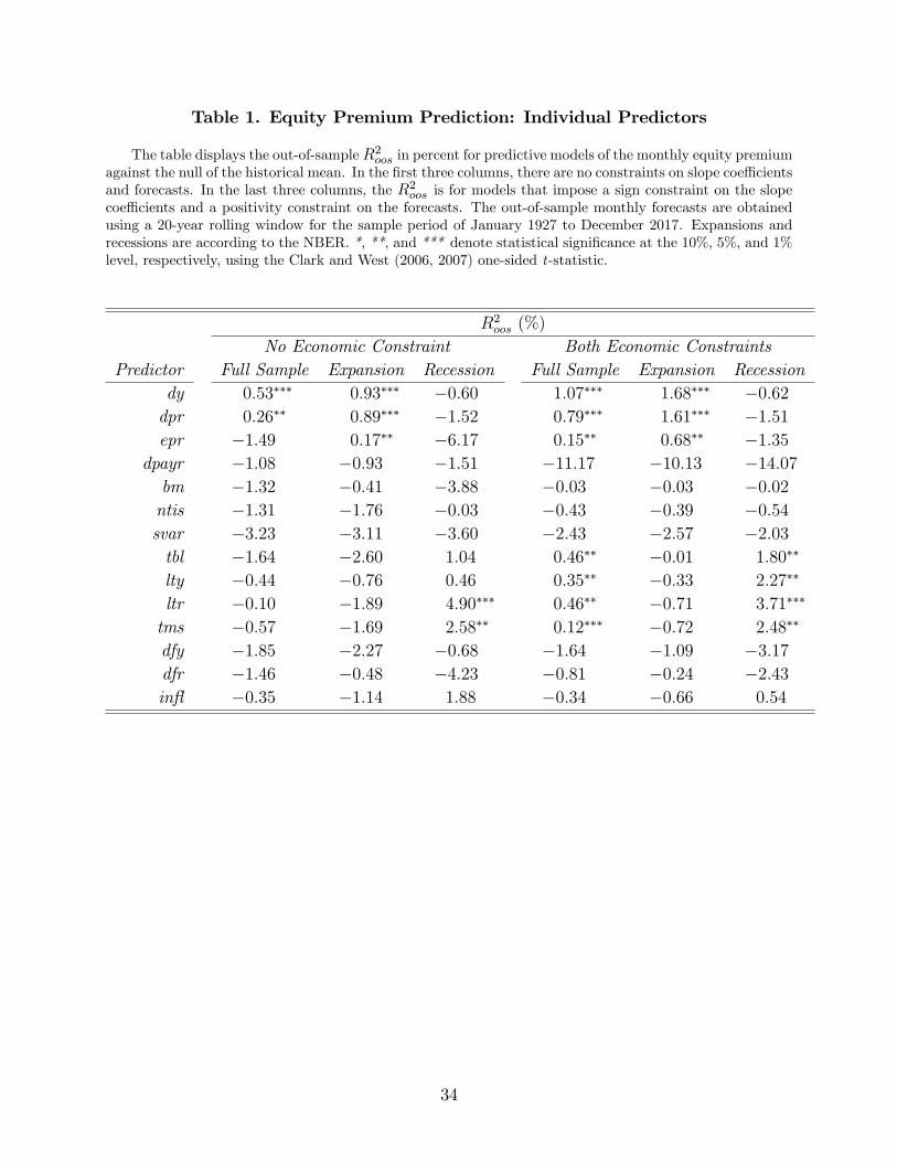
Table 1. Equity Premium Prediction: Individual Predictors
The table displays the out-of-sampleR2oos in percent for predictive models of the monthly equity premiumagainst the null of the historical mean. In the first three columns, there are no constraints on slope coeffi cientsand forecasts. In the last three columns, the R2oos is for models that impose a sign constraint on the slopecoeffi cients and a positivity constraint on the forecasts. The out-of-sample monthly forecasts are obtainedusing a 20-year rolling window for the sample period of January 1927 to December 2017. Expansions andrecessions are according to the NBER. *, **, and *** denote statistical significance at the 10%, 5%, and 1%level, respectively, using the Clark and West (2006, 2007) one-sided t-statistic.
R2oos (%)
No Economic Constraint Both Economic ConstraintsPredictor Full Sample Expansion Recession Full Sample Expansion Recession
dy 0.53∗∗∗ 0.93∗∗∗ −0.60 1.07∗∗∗ 1.68∗∗∗ −0.62
dpr 0.26∗∗ 0.89∗∗∗ −1.52 0.79∗∗∗ 1.61∗∗∗ −1.51
epr −1.49 0.17∗∗ −6.17 0.15∗∗ 0.68∗∗ −1.35
dpayr −1.08 −0.93 −1.51 −11.17 −10.13 −14.07
bm −1.32 −0.41 −3.88 −0.03 −0.03 −0.02
ntis −1.31 −1.76 −0.03 −0.43 −0.39 −0.54
svar −3.23 −3.11 −3.60 −2.43 −2.57 −2.03
tbl −1.64 −2.60 1.04 0.46∗∗ −0.01 1.80∗∗
lty −0.44 −0.76 0.46 0.35∗∗ −0.33 2.27∗∗
ltr −0.10 −1.89 4.90∗∗∗ 0.46∗∗ −0.71 3.71∗∗∗
tms −0.57 −1.69 2.58∗∗ 0.12∗∗∗ −0.72 2.48∗∗
dfy −1.85 −2.27 −0.68 −1.64 −1.09 −3.17
dfr −1.46 −0.48 −4.23 −0.81 −0.24 −2.43
infl −0.35 −1.14 1.88 −0.34 −0.66 0.54
34

Table 2. Equity Premium Prediction: Simple Forecast Combinations
The table reports the out-of-sample R2oos in percent for predictive models of the monthly equity premiumagainst the null of the historical mean. The R2oos is for models that impose a sign constraint on the slopecoeffi cients and a positivity constraint on the forecasts. The out-of-sample monthly forecasts are obtainedusing a 20-year rolling window for the sample period of January 1927 to December 2017. Expansions andrecessions are according to the NBER. *, **, and *** denote statistical significance at the 10%, 5%, and 1%level, respectively, using the Clark and West (2006, 2007) one-sided t-statistic.
R2oos (%)
Predictor Full Sample Expansion Recession
Two individual predictorsdy 1.07∗∗∗ 1.68∗∗∗ −0.62
tbl 0.46∗∗ −0.01 1.80∗∗
Simple mean combination with two predictorsdy + tbl 1.54∗∗∗ 1.63∗∗∗ 1.28∗
Ex-post timing using the true recession dummydy + tbl 1.71∗∗∗ 1.68∗∗∗ 1.80∗∗
Standard forecast combinationall 14 predictors 0.83∗∗∗ 0.99∗∗∗ 0.39
35

Table 3. Equity Premium Prediction: More Forecast Combinations
The table displays the out-of-sampleR2oos in percent for predictive models of the monthly equity premiumagainst the null of the historical mean. The formation of forecasts is as described in Table 2. The sampleperiod ranges from January 1927 to December 2017. Expansions and recessions are according to the NBER.*, **, and *** denote statistical significance at the 10%, 5%, and 1% level, respectively, using the Clark andWest (2006, 2007) one-sided t-statistic.
R2oos (%)
Predictor Full Sample Expansion Recession
Mean combinations with two predictorsdy + tbl 1.54∗∗∗ 1.63∗∗∗ 1.28∗
dy + tms 1.54∗∗∗ 1.57∗∗∗ 1.47∗
dy + lty 1.40∗∗∗ 1.41∗∗∗ 1.39∗
dy + ltr 1.51∗∗∗ 1.29∗∗∗ 2.13∗
dpr + tbl 1.30∗∗∗ 1.51∗∗∗ 0.72
dpr + tms 1.37∗∗∗ 1.52∗∗∗ 0.95
dpr + lty 1.19∗∗∗ 1.30∗∗∗ 0.87
dpr + ltr 1.34∗∗∗ 1.21∗∗∗ 1.68∗
epr + tbl 1.02∗∗∗ 1.03∗∗∗ 0.99∗
epr + tms 1.23∗∗∗ 1.16∗∗∗ 1.43∗∗
epr + lty 0.78∗∗∗ 0.73∗∗ 0.93∗
epr + ltr 1.05∗∗∗ 0.64∗∗ 2.19∗∗∗
Mean combinations with three predictorsdy + tbl + dpr 1.43∗∗∗ 1.77∗∗∗ 0.47
dy + tbl + epr 1.41∗∗∗ 1.63∗∗∗ 0.81∗
dy + tbl + tms 1.62∗∗∗ 1.53∗∗∗ 1.86∗∗
dy + tbl + lty 1.36∗∗∗ 1.23∗∗∗ 1.74∗∗
dy + tbl + ltr 1.66∗∗∗ 1.35∗∗∗ 2.53∗∗∗
Mean combination for typical idiosyncratic predictorsdy + epr 1.04∗∗∗ 1.59∗∗∗ −0.49
Mean combination for typical systematic predictorstbl + tms + ltr 1.33∗∗∗ 0.61∗∗ 3.35∗∗∗
Mean combination for idiosyncratic + systematic predictorsdy + epr + tbl + tms + ltr 1.68∗∗∗ 1.48∗∗∗ 2.24∗∗∗
36

Table 4. Two-Predictor Forecast Combinations
The table displays the percent out-of-sample 2 and the model rank for two-predictor forecast combinations. The formation of forecasts is asdescribed in Table 2 using the initial in-sample period of January 1927 to December 1946. The training period is the initial out-of-sample periodover which models are evaluated. All training periods begin with the first out-of-sample forecast in January 1947. The forecasting period is the finalout-of-sample period over which models are implemented. All forecasting periods end with the last out-of-sample forecast in December 2017. PanelA reports the percent out-of-sample 2. Panel B reports the rank of each model based on its
2 relative to all other models. The average rank
is the rank across all training periods or all forecasting periods or both. The table suppresses evidence of statistical significance to conserve space.
Panel A: 2 (%)dy dy dy dy dpr dpr dpr dpr epr epr epr epr ALL
Training Period + + + + + + + + + + + + 14Begin End tbl tms lty ltr tbl tms lty ltr tbl tms lty ltr predictors194701 196612 254 244 209 260 193 195 160 234 191 161 091 159 145
194701 197612 285 293 249 296 231 253 202 266 157 178 092 157 146
194701 198612 189 205 160 214 153 181 128 191 091 141 041 122 127
194701 199612 149 147 114 157 119 128 088 148 074 100 023 099 096
194701 200612 162 161 135 161 138 149 114 147 100 126 059 107 093
Forecasting PeriodBegin End196701 201712 128 131 122 117 113 122 108 107 078 113 075 090 067
197701 201712 072 068 072 053 066 064 066 050 067 089 070 072 044
198701 201712 114 096 118 078 104 086 108 067 114 102 122 084 033
199701 201712 164 169 195 116 152 157 184 103 162 172 194 117 057
200701 201712 114 104 170 090 087 077 145 062 112 107 177 091 032
37

Table 4 (continued)
Panel B: Rank of Each Model based on 2 Relative to All Other Modelsdy dy dy dy dpr dpr dpr dpr epr epr epr epr ALL
Training Period + + + + + + + + + + + + 14Begin End tbl tms lty ltr tbl tms lty ltr tbl tms lty ltr predictors194701 196612 2 3 5 1 7 6 10 4 8 9 13 11 12
194701 197612 3 2 6 1 7 5 8 4 10 9 13 11 12
194701 198612 4 2 6 1 7 5 9 3 12 8 13 11 10
194701 199612 2 4 7 1 6 5 11 3 12 8 13 9 10
194701 200612 1 3 7 2 6 4 9 5 11 8 13 10 12
Average rank 24 28 62 12 66 5 94 38 106 84 13 104 112
Rank of average rank 2 3 6 1 7 5 9 4 11 8 13 10 12
Forecasting PeriodBegin End196701 201712 2 1 3 5 6 4 8 9 11 7 12 10 13
197701 201712 2 6 3 11 9 10 8 12 7 1 5 4 13
198701 201712 4 8 2 11 6 9 5 12 3 7 1 10 13
199701 201712 6 5 1 11 9 8 3 12 7 4 2 10 13
200701 201712 4 7 2 9 10 11 3 12 5 6 1 8 13
Average rank 36 54 22 94 8 84 54 114 66 5 42 84 13
Rank of average rank 2 5 1 11 8 9 5 12 7 4 3 9 13
All Training andForecasting Periods
Average rank 3 41 42 53 73 67 74 76 86 67 86 94 121
Rank of average rank 1 2 3 4 7 5 8 9 10 5 10 12 13
38

Table 5. Portfolio Performance
The table reports the out-of-sample portfolio performance for a mean-variance investor, who each monthrebalances her portfolio by investing in one risky asset (S&P 500) and the riskless rate (T-bill). The investorhas a degree of relative risk aversion equal to 2 (Panel A) or 6 (Panel B). ∆CER is the gain in the percentannualized Certainty Equivalent Return (CER) for switching from the forecasts of the benchmark to theforecasts generated by the alternative model. SR is the annualized Sharpe ratio. EPM is the EconomicPerformance Measure. TO is the ratio of the average turnover of the portfolio generated by the forecastsof the alternative model divided by the average turnover of the portfolio generated by the benchmark. Forthe historical mean benchmark, we report the level of CER and the average turnover for that portfolio. Thesuperscripts *, **, and *** denote statistical significance at the 10%, 5%, and 1% level, respectively, usingthe Ledoit and Wolf (2008) bootstrap two-sided test of whether the Sharpe ratio of a model is different fromthe benchmark. The last two columns are the annual percent ∆CER assuming a proportional transactioncost of either 50 or 100 basis points. The formation of forecasts is as described in Table 2. The sampleperiod ranges from January 1927 to December 2017.
Panel A: RRA=2 (γ = 2)∆CER (%) ∆CER (%)
Predictor Full Exp. Rec. SR EPM TO c = 50 c = 100Historical mean 9.47 11.89 −4.88 0.48 0.48 0.06 9.36 9.24
Two individual predictorsdy 1.78 2.09 0.63 0.61∗ 0.60 2.12 1.78 1.37tbl 0.18 −1.60 10.71 0.53 0.52 1.42 −0.06 −0.30
Simple mean combination with two predictorsdy + tbl 1.16 1.06 1.71 0.55∗ 0.54 1.64 0.86 0.56
Ex-post timing using the true recession dummydy + tbl 3.33 2.09 10.71 0.74∗∗∗ 0.73 2.33 2.81 2.27
Standard forecast combinationall 14 predictors 0.93 0.87 1.22 0.52 0.51 1.30 0.86 0.79
Panel B: RRA=6 (γ = 6)Historical mean 5.34 6.76 −3.08 0.46 0.46 0.03 5.18 5.01
Two individual predictorsdy 0.88 2.02 −5.92 0.53 0.51 2.52 0.56 0.24tbl 1.61 0.38 8.87 0.59 0.56 1.42 1.50 1.40
Simple mean combination with two predictorsdy + tbl 2.10 1.84 3.63 0.64∗∗∗ 0.62 1.75 1.93 1.75
Ex-post timing using the true recession dummydy + tbl 3.01 2.02 8.87 0.74∗∗∗ 0.73 2.66 2.65 2.29
Standard forecast combinationall 14 predictors 0.52 0.89 −1.73 0.51 0.50 1.62 0.37 0.23
39

Table 6. Timing the Business Cycle
The table displays the out-of-sampleR2oos in percent for predictive models of the monthly equity premiumagainst the null of the historical mean. The formation of forecasts is as described in Table 2. The sampleperiod ranges from June 1947 to December 2017 so that the first forecast is for June 1967. Expansions andrecessions are according to the NBER. *, **, and *** denote statistical significance at the 10%, 5%, and 1%level, respectively, using the Clark and West (2006, 2007) one-sided t-statistic.
R2oos (%)
Predictor Full Sample Expansion Recession
Two individual predictorsdy 0.46∗∗ 1.09∗∗∗ −1.04
tbl 0.87∗∗ 0.19∗ 2.51∗∗
Simple mean combination with two predictorsdy + tbl 1.38∗∗∗ 1.39∗∗∗ 1.34∗
Ex-ante timing using the forecasted recession dummydy + tbl 0.98∗∗∗ 0.34∗∗ 3.47∗∗
Ex-ante timing using the HP output gapdy + tbl 0.47∗∗ −0.55 4.45∗∗∗
Ex-ante timing using the HP ∆(output gap)
dy + tbl 2.06∗∗∗ 0.43∗∗ 8.50∗∗∗
Ex-ante timing using the HP 3-month ∆(output gap)
dy + tbl 1.63∗∗∗ 0.70∗∗ 5.29∗∗∗
40
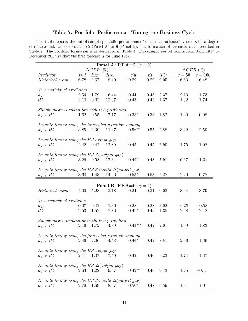
Table 7. Portfolio Performance: Timing the Business Cycle
The table reports the out-of-sample portfolio performance for a mean-variance investor with a degreeof relative risk aversion equal to 2 (Panel A) or 6 (Panel B). The formation of forecasts is as described inTable 2. The portfolio formation is as described in Table 4. The sample period ranges from June 1947 toDecember 2017 so that the first forecast is for June 1967.
Panel A: RRA=2 (γ = 2)∆CER (%) ∆CER (%)
Predictor Full Exp. Rec. SR EP TO c = 50 c = 100Historical mean 6.78 9.67 −8.40 0.29 0.29 0.05 6.63 6.48
Two individual predictorsdy 2.54 1.79 6.44 0.44 0.43 2.37 2.13 1.73tbl 2.10 0.02 12.97 0.43 0.42 1.37 1.92 1.74
Simple mean combination with two predictorsdy + tbl 1.62 0.55 7.17 0.38∗ 0.38 1.82 1.30 0.98
Ex-ante timing using the forecasted recession dummydy + tbl 3.85 2.39 11.47 0.56∗∗ 0.55 2.88 3.22 2.59
Ex-ante timing using the HP output gapdy + tbl 2.42 0.42 12.89 0.45 0.45 2.90 1.75 1.08
Ex-ante timing using the HP ∆(output gap)dy + tbl 3.26 0.58 17.34 0.49∗ 0.48 7.91 0.97 −1.34
Ex-ante timing using the HP 3-month ∆(output gap)dy + tbl 3.60 1.43 14.96 0.53∗ 0.53 5.28 2.20 0.78
Panel B: RRA=6 (γ = 6)Historical mean 4.09 5.28 −2.18 0.24 0.24 0.03 3.94 3.79
Two individual predictorsdy 0.07 0.42 −1.86 0.28 0.28 3.02 −0.25 −0.58tbl 2.53 1.52 7.86 0.47∗ 0.45 1.35 2.48 2.42
Simple mean combination with two predictorsdy + tbl 2.16 1.72 4.39 0.43∗∗∗ 0.42 2.01 1.99 1.83
Ex-ante timing using the forecasted recession dummydy + tbl 2.46 2.06 4.53 0.46∗ 0.42 3.51 2.06 1.66
Ex-ante timing using the HP output gapdy + tbl 2.11 1.07 7.50 0.42 0.40 3.23 1.74 1.37
Ex-ante timing using the HP ∆(output gap)dy + tbl 2.63 1.22 9.97 0.49∗∗ 0.46 9.73 1.25 −0.15
Ex-ante timing using the HP 3-month ∆(output gap)dy + tbl 2.79 1.69 8.57 0.50∗ 0.48 6.59 1.91 1.01
41

Table 8. The Financial Cycle
The table displays the out-of-sampleR2oos in percent for predictive models of the monthly equity premiumagainst the null of the historical mean. The formation of forecasts is as described in Table 2. The sampleperiod ranges from January 1940 to December 2017 so that the first forecast is for January 1960. Expansionsand recessions are according to the NBER. Financial cycle upturns and downturns are defined as in Claessens,Kose, and Terrones (2012). *, **, and *** denote statistical significance at the 10%, 5%, and 1% level,respectively, using the Clark and West (2006, 2007) one-sided t-statistic.
R2oos (%)
Expansion/ Recession/Predictor Full Sample Upturn Downturn
Business Cycledy 0.83∗∗ 1.64∗∗∗ −1.30
tbl 1.02∗∗∗ 0.59∗∗ 2.14∗∗
Mean: dy + tbl 1.58∗∗∗ 1.81∗∗∗ 1.00∗
Financial Cycledy 0.83∗∗ 1.29∗∗∗ −0.28
tbl 1.02∗∗∗ 0.23∗∗ 2.90∗∗∗
Mean: dy + tbl 1.58∗∗∗ 1.40∗∗∗ 2.02∗∗
Business and Financial Cycledy 0.83∗∗ 0.38∗∗ 1.35
tbl 1.02∗∗∗ 0.61∗∗ 3.30∗∗
Mean: dy + tbl 1.58∗∗∗ 1.20∗∗∗ 3.08∗∗
42

Table 9. International Evidence
The table displays the out-of-sample R2oos in percent for four additional countries plus the US. TheR2oos is for models that impose a sign constraint on the slope coeffi cients and a positivity constraint on theforecasts. The out-of-sample monthly forecasts are obtained using a 20-year rolling window. Expansions andrecessions are according to the NBER. *, **, and *** denote statistical significance at the 10%, 5%, and 1%level, respectively, using the Clark and West (2006, 2007) one-sided t-statistic. Ex-post timing uses the truerecession dummy, whereas ex-ante timing uses the HP output gap.
Panel A: Canada, Dec 1969 - Dec 2017Predictor Full Sample Expansion Recessiondy −0.64 2.67∗∗ −3.14tbl −1.26 −5.55 1.97∗
Mean: dy + tbl 0.15 0.31 0.02Ex-post: dy + tbl 2.27∗∗∗ 2.67∗∗ 1.97∗
Ex-ante: dy + tbl 3.11∗∗∗ 3.95∗∗∗ 2.48∗∗
Panel B: UK, Dec 1964 - Dec 2017dy −0.79 0.28∗ −2.11tbl −1.89 −3.78 0.44∗
Mean: dy + tbl 0.05 0.22 −0.17Ex-post: dy + tbl 0.35∗ 0.28∗ 0.44∗
Ex-ante: dy + tbl 0.43∗ −0.87 2.02∗∗
Panel C: Germany, Dec 1972 - Dec 2017dy 0.39∗ −2.82 0.46∗∗
tbl −0.41 −3.04 −0.35Mean: dy + tbl 0.00 −2.91 0.05Ex-post: dy + tbl −0.40 −2.82 −0.35Ex-ante: dy + tbl −0.40 −2.74 −0.35
Panel D: Japan, Jan 1986 - Dec 2017dy −0.48 3.94∗ −0.97tbl 0.23 −11.13 1.49∗
Mean: dy + tbl 0.26 −1.55 0.46∗
Ex-post: dy + tbl 1.73∗ 3.94∗ 1.49∗
Ex-ante: dy + tbl 1.55∗ 3.72∗ 1.31∗
Panel E: USA, Jan 1964 - Dec 2017dy 1.14∗∗∗ 1.25∗∗∗ 0.66tbl 0.16 −0.53 2.90∗∗
Mean: dy + tbl 1.12∗∗∗ 0.90∗∗ 2.01∗∗∗
Ex-post: dy + tbl 1.58∗∗∗ 1.25∗∗∗ 2.90∗∗
Ex-ante: dy + tbl 0.70∗ 0.15 2.90∗∗
43

Figure 1. Out-of-sample equity premium prediction
The figure displays the performance of selected empirical models in out-of-sample equity premium prediction. Each graph shows the differenceof the cumulative squared error of the null (historical mean) minus the cumulative squared error of the alternative. The grey areas indicateNBER-defined recessions. The out-of-sample monthly forecasts are obtained with rolling regressions using a window of 20 years for the sampleperiod of January 1927 to December 2017.
44

Figure 2. Two-Predictor Forecast Combinations based on the Dividend Yield
The figure displays the out-of-sample performance over time in equity premium prediction of two-predictor forecast combinations based onthe dividend yield. In each graph, the solid blue line is the benchmark two-predictor model that combines the forecasts of the dividend yield(dy) and the short rate (tbl). The red dashed line is for the alternative two-predictor model. In the bottom right graph, the alternative modelis the forecast combination of all 14 predictors. Each line represents the difference of the cumulative squared error of the null (historicalmean) minus the cumulative squared error of the selected model. Hence a positive value indicates that the model performs better than thehistorical mean. The grey areas indicate NBER-defined recessions. The out-of-sample monthly forecasts are obtained with rolling regressionsusing a window of 20 years for the sample period of January 1927 to December 2017.
45

Figure 3. Two-Predictor Forecast Combinations based on the Dividend-Price Ratio
The figure displays the out-of-sample performance over time in equity premium prediction of two-predictor forecast combinations based onthe dividend-price ratio. In each graph, the solid blue line is the benchmark two-predictor model that combines the forecasts of the dividendyield (dy) and the short rate (tbl). The red dashed line is for the alternative two-predictor model. Each line represents the difference ofthe cumulative squared error of the null (historical mean) minus the cumulative squared error of the selected model. Hence a positive valueindicates that the model performs better than the historical mean. The grey areas indicate NBER-defined recessions. The out-of-samplemonthly forecasts are obtained with rolling regressions using a window of 20 years for the sample period of January 1927 to December 2017.
46

Figure 4. Two-Predictor Forecast Combinations based on the Earnings-Price Ratio
The figure displays the out-of-sample performance over time in equity premium prediction of two-predictor forecast combinations based onthe earnings-price ratio. In each graph, the solid blue line is the benchmark two-predictor model that combines the forecasts of the dividendyield (dy) and the short rate (tbl). The red dashed line is for the alternative two-predictor model. Each line represents the difference ofthe cumulative squared error of the null (historical mean) minus the cumulative squared error of the selected model. Hence a positive valueindicates that the model performs better than the historical mean. The grey areas indicate NBER-defined recessions. The out-of-samplemonthly forecasts are obtained with rolling regressions using a window of 20 years for the sample period of January 1927 to December 2017.
47