ercolation, p - technische universität chemnitz · ercolation p and tum-hall quan ransition t 3...

$: ercolation, P - Technische Universität Chemnitz · ercolation P and tum-Hall Quan ransition T 3 increases as h M (N) i / D, where D is the fractal dimension of cluster. As in y an$
Per olation, Renormalization and the

Quantum-Hall Transition

Rudolf A. R�omer

Institut f�ur Physik, Te hnis he Universit�at, 09107 Chemnitz, Germany

Abstra t. In this arti le, I give a pedagogi al introdu tion and overview of per olation

theory. Spe ial emphasis will be put on the review of some of the most prominent of the

algorithms that have been devised to study per olation numeri ally. At the entral stage

shall be the real-spa e renormalization group treatment of the per olation problem. As

a rather novel appli ation of this approa h to per olation, I will review re ent results

using similar real-spa e renormalization ideas that have been applied to the quantum

Hall transition.

1 Introdu tion

Imagine a large hessboard, su h as o asionally found in a park. It is fall, and

all the master players have ed the old a long time ago. You are taking a walk

and enjoy the beautiful sunny afternoon, all the olors of the Indian summer in

the trees and in the falling leaves around you. Looking at the hessboard, you

see that some squares are already full of leaves, while others are still empty [1℄.

The pattern of the squares whi h are overed by leaves seems rather random. As

you try to ross the hessboard, you see that there is a way to get from one side

of the board to the opposite side by walking on leaf- overed squares only. This

is per olation | nearly.

Before ontinuing and explaining in detail what per olation is about, let me

outline the ontent of this paper. In Se t. 2, I will review some of the most

prominent and interesting results on lassi al per olation. Per olation theory is

at the heart of many phenomena in statisti al physi s that are also topi s in this

book. Beyond the exa t solutions of per olation in d = 1 and d =1 dimensions,

further exa t solutions in 2 � d < 1 only rarely exist. Thus omputational

methods, using high-performan e omputers and algorithms are needed for fur-

ther progress and in Se ts. 2.2 { 2.4, I explain in detail some of these algorithms.

Se tion 3 is devoted to the real-spa e renormalization group (RG) approa h to

per olation. This provides an independent and very suggestive method of an-

alyti ally omputing results for the per olation problem as well as a further

numeri al algorithm.

While many appli ations of per olation theory are mainly on erned with

problems of lassi al statisti al physi s, I will show in Se t. 4 that the per olation

approa h an give useful information also at the quantum s ale. In parti ular,

I will show that aspe ts of the quantum Hall (QH) e�e t an be understood by

a suitably generalized renormalization pro edure of bond per olation in d = 2.

2 Rudolf A. R�omer

This appli ation allows the omputation of riti al exponents and ondu tan e

distributions at the QH transition and also opens the way for studies of s ale-

invariant, experimentally relevant ma ros opi inhomogeneities. I summarize in

Se t. 5.

2 Per olation

2.1 The Physi s of Conne tivity

From the hessboard example given above, we realize that the per olation prob-

lem deals with the spatial onne tivity of o upied squares instead of simply

ounting whether the number of su h squares has the majority of all squares.

Then the obvious question to ask is: How many leaves are usually needed in

order to allow passage a ross the board? Sin e leaves normally do not intera t

with ea h other, and fri tion-related for es an be assumed small ompared to

wind for es, we an model the situation by assuming that the leaves are ran-

domly distributed on the board. Then we an de�ne an o upation probability

p as being the probability that a site is o upied (by at least one leaf). Thus our

question an be rephrased in modern physi s terminology as: Is there a threshold

value p

at whi h there is a spanning luster of o upied sites a ross an in�nite

latti e?

The �rst time this question was asked and the term per olation used was in

the year 1957 in publi ations of Broadbent and Hammersley [2{4℄. Sin e then a

multitude of resear h arti les, reviews and books have appeared on this subje t.

Certainly among the most readable su h publi ations is the 1995 book by Stau�er

and Aharony [5℄, where alsomost of the relevant resear h arti les have been ited.

Let me here brie y summarize some of the highlights that have been dis overed

in the nearly 50 years of resear h on per olation.

The per olation problem in d = 1 an be solved exa tly. Sin e the number of

empty sites in a hain of length L is (1� p)L, there is always a �nite probability

for �nding su h an empty site in the in�nite luster at L ! 1 and thus the

per olation threshold is p

= 1. De�ning a orrelation fun tion g(r) / exp(�r=�)

whi h measures the probability that a site at distan e r from an o upied site at

0 belongs to the same luster, we easily �nd g(r) = p

r

and thus � = �1= lnp �

(p

� p)

�1

. Thus lose to the per olation threshold, the orrelation length �

diverges with an exponent � = 1.

In d = 2, the per olation problem provides perhaps the simplest example of

a se ond-order phase transition. The order parameter of this transition is the

probability P (p) that an arbitrary site in the in�nite latti e is part of an in�nite

luster [6℄, i.e.,

P (p) =

�

0; p � p

;

(p� p

)

�

; p > p

(1)

and � is a riti al exponent similar to the exponent � of the orrelation length.

The distribution of the sites in an in�nite luster at the per olation threshold

an be des ribed as a fra tal [7℄, i.e., its average size M in boxes of length N

Per olation and Quantum-Hall Transition 3

in reases as hM(N)i / N

D

, where D is the fra tal dimension of the luster. As

in any se ond-order phase transition, mu h insight an be gained by a �nite-size

s aling analysis [7,8℄. In parti ular, the exponents introdu ed above are related

a ording to the s aling relation � = (d�D)� [5℄. Furthermore, it has been shown

to an astonishing degree of a ura y, that the values of the exponents and the

relations between them are independent of the type of latti e onsidered, i.e.,

square, triangular, honey omb, et ., and also whether the per olation problem is

de�ned for sites or bonds (see Fig. 1). This independen e is alled universality. In

the following, we will see that the universality does not apply for the per olation

threshold p

. Thus it is of importan e to note that p

for site per olation on the

triangular latti e and bond per olation on the square latti e is known exa tly:

p

= 1=2. Espe ially the bond per olation problem has re eived mu h attention

also by mathemati ians [9℄.

Fig. 1. Site (left) and bond (right) per olation on a square latti e. In site per ola-

tion, the sites of a latti e are o upied randomly and per olation is de�ned via, say,

nearest-neighbor sites. In bond per olation, the bonds onne ting the sites are used

for per olation. The thin outlines de�ne the 3 lusters in ea h panel. The solid outline

indi ates the per olating luster

For higher dimensions, mu h of this pi ture remains un hanged, although

the values of p

and the riti al exponents hange. The upper riti al dimension

orresponds to d = 6 su h that mean �eld theory is valid for d � 6 with exponents

as given in Table 1.

Appli ations of per olation theory are numerous [10℄. It is intimately on-

ne ted to the theory of phase transitions as dis ussed in [8,11℄. The onne tivity

problem is also relevant for di�usion in disordered media [7,12℄ and networks [13℄.

A simple model of forest �res is based on per olation ideas [14℄ and even models

of sto k market u tuations [15℄ have been devised using ideas of per olation

[16℄. Per olation is therefore a well-established �eld of statisti al physi s and it


Table 1. Criti al exponents � and � and fra tal dimension D for di�erent spatial

dimensions. For a more omplete list see [5℄.

Exponent d = 2 d = 3 d = 4 d = 5 d = 6� �

� 4=3 0:88 0:68 0:57 1=2 + 5�=84

� 5=36 0:41 0:64 0:84 1� �=7

D(p = p

) 91=48 2:53 3:06 3:54 4� 10�=21

D(p < p

) 1:56 2 12=5 2:8 �

D(p > p

) 2 3 4 5 �

ontinues its vital progress with more than 230 publi ations in the ond-mat

ar hives [17℄ alone.

2.2 The Coloring Algorithm

As stated above, there are only few exa t results available in per olation in d � 2.

Thus in order to pro eed further, one has to use omputational methods.

The standard numeri al algorithm of per olation theory is due to Hoshen

and Kopelman [18℄. Its advantage is due to the fa t that it allows to analyze

whi h site belongs to whi h luster without having to store the omplete latti e.

Furthermore, this is being done in one sweep a ross the latti e, thus redu ing

omputer time.

At the heart of the Hoshen-Kopelman algorithm is a bookkeeping me hanism

[5℄. Look at the site per olation luster in Fig. 1. Going from left to right and

top to bottom through the luster, we give ea h site a label (or olor) as shown

in Fig. 2. If its top or left neighbor is already o upied, then the new site belongs

to the same luster and gets the same label. Otherwise we hoose a new label. In

this way we an pro eed through the luster until we rea h a problem in line 3

as shown in the left olumn of Fig. 2. A ording to our above rule the new site,

indi ated by the bold question mark, an be either 2 or 4. This indi ates that

all sites previously labelled by 2 and 4 a tually belong to the same luster. Thus

we now introdu e an index Id(�) for ea h luster label and de�ne it su h that

the index of a super uous label, say 4, points to the right label, viz. Id(4) = 2.

Pro eeding with our analysis into the 4th row of the latti e, we see in the enter

olumn of Fig. 2 that we again have to adjust our index at the position indi ated

in bold. Instead of labeling this site as 4, we hoose 2 � Id(4). And onsequently,

Id(3) = 2. In this way, we an easily he k whether a luster per olates from top

to bottom of the latti e by simply he king whether the label of any o upied

site in the bottom row of the latti e has an index equal to any of the labels

in the top row. Furthermore, in addition to the top row, we only need to store

the row presently under onsideration and its prede essor. Thus the storage

requirement is linear in latti e size L and not L

2

as it would be if we were to


store the full latti e. Last, the algorithm an also give information about all

lusters, say, if needed for a fra tal analysis of the non-per olating lusters. A

Java implementation of su h a oloring algorithm an be found in Ref. [19℄.

1 1 2

1 2 2

3 4 ?

� � �

� � �

1 1 2

1 2 2

3 4 4

3 3 ?

� � �

1 1 2

1 2 2

3 4 4

3 3 2

2 5 5

Id(1) = 1

Id(2) = 2

Id(3) = 3

Id(4) = 2

Id(1) = 1

Id(2) = 2

Id(3) = 2

Id(4) = 2

Id(1) = 1

Id(2) = 2

Id(3) = 2

Id(4) = 2

Id(5) = 5

Fig. 2. S hemati des ription of the Hoshen-Kopelman oloring algorithm of the site

per olation problem on a square latti e as shown in Fig. 1. � denotes an o upied site,

the numbers denote the luster labels. The horizontal lines bra ket the urrent and the

previous row

2.3 The Growth Algorithm

When we want to study primarily the geometri al properties of per olation lus-

ters, another algorithm is more suitable whi h allows to generate the desired

luster stru ture dire tly. This algorithm is due to Leath [20℄ and works by a

luster-growth strategy. The idea of the algorithm is that we put an o upied

site in the enter of an otherwise empty latti e. Then we identify its nearest-

neighbor sites as shown in Fig. 3. Next we o upy these sites a ording to the

desired per olation probability p. We identify the new, yet unde ided nearest-

neighbor sites, o upy these again with probability p and repeat the pro edure.

The luster ontinues to grow until either all sites at the boundary are uno -

upied or the luster has rea hed the boundary of the latti e. For p < p

, the

growth usually stops after a few iterations, while for p > p

, per olating lusters

are generated almost always. Thus besides giving information about the fra tal

stru ture of the per olating lusters, the Leath algorithm an also be used to

estimate the value of p

. A Java implementation of the Leath algorithm an be

found in Refs. [21,22℄.


� � � � �

� � � � �

� � � � �

� � � � �

� � � � �

� � � � �

� � Æ � �

� Æ � � �

� � � � �

� � � � �

� � � � �

� � Æ � �

� Æ � � Æ

� � � Æ �

� � Æ � �

Fig. 3. S hemati des ription of the �rst three steps in the Leath growth algorithm

of the site per olation luster of Fig. 1. �, Æ, and � denote an o upied, empty, and

unde ided site

2.4 The Frontier Algorithm

As we have seen in the last se tion, the outer frontier of the per olation luster

is well de�ned. The fra tal properties of this hull an be measured [23,24℄ and

shown to yield D

h

= 1:74 � 0:02. This suggests yet another algorithm for the

determination of p

[25,26℄: Generate a latti e with a onstant gradientrp of the

o upation probability p as shown in Fig. 4. By an algorithm similar to the one

��

��

��

��

��

��

��

��

��

��

��

��

��

��

��

��

p=0

p=1

Fig. 4. An example for gradient per olation. All sites at p = 1 (p = 0) are o upied

(empty). The 15 large ir les orrespond to o upied sites. The 8 light shaded sites

belong to the frontier, whereas the 7 dark shaded sites are part of the interior of the

luster or belong to other lusters. The 5 small ir les orrespond to sites in the empty

frontier. The dashed line indi ates the frontier generating walk. Note that only the 14

sites with solid ir les have a tually been visited. The 6 other ir les are shown here

just for larity and need not be generated. A ording to (2), we have p

= (8 � 0:4375+

5 � 0:75)=13 = 0:55769

used in omputing the hull of the per olating luster, one traverses the frontier


Table 2. Various urrent estimates of p

for site and bond per olation on di�erent

latti es in d = 2 [28{33℄. Exa tly known values are emphasized. The latti es are lassi-

�ed a ording to their number of �rst, se ond and more nearest-neighbors. The upper

index gives the orresponding number in the dual latti e

latti e site p

bond p

3; 12

2

0.807 904

4; 6; 12 0:747 806

4; 8

2

0:729 724

6

3

honey omb 0:697 043 0.652 703

3; 6; 3; 6 Kagom�e 0.652 703 0:524 4

4

4

di e 0:584 8 0:475 4

3; 4; 6; 4 0:621 819

4

4

square 0:592 746 0 0.500 000

3

4

; 6 0:579 498

3

2

; 4; 3; 4 0:550 806

3

3

; 4

2

0:550 213

3

6

triangular 0.500 000 0.347 296

of the o upied luster and determines whi h sites belong to it and whi h belong

to the empty luster [24{26℄. Then a very reliable estimate for the per olation

threshold an be omputed as

p

=

N

o

p

o

+N

e

p

e

N

o

+N

e

; (2)

whereN

o;e

denotes the number of sites in the o upied (empty) frontier and p

o; e

is the mean height of the asso iated frontiers, respe tively. Note that instead of

a tually generating the per olation latti e, the algorithm instead pro eeds by just

generating the sites needed for the onstru tion of the frontier. Thus instead of

dealing with, say, O(L

2

) sites as in the Hoshen-Kopelman and Leath algorithms

for a latti e in d = 2, one only needs O(L) sites in the present algorithm [27℄.

This redu es omputer time and estimates for p

in a large variety of latti es

an be obtained with high a ura y [28{33℄ as shown in Table 2.

3 Real-Spa e Renormalization

3.1 Making Use of Self-Similarity

As mentioned in Se t. 2, the transition at p

orresponds to a se ond-order phase

transition and the orrelation length � is in�nite. There is no parti ular length


s ale in the system and all lusters are statisti ally similar to ea h other. This

self-similarity [7℄ is at the bottom of the renormalization des ription just as for

the fra tal analysis of the per olation lusters.

We may use the self-similarity in the following way. Let us repla e a suitable

olle tion of sites by super-sites and then study per olation of the super-latti e

[34{38℄. In general, the o upation probability p

0

of the super-latti e will be

di�erent from the original p. Furthermore, if the extent of the olle tion of sites

in the latti e was b, then the super-latti e will have a latti e onstant b. Thus

� = b�

0

and with � / jp� p

j

��

, we �nd

bjp

0

� p

j

��

� jp� p

j

��

(3)

and onsequently,

� =

log b

log

dp

0

dp

: (4)

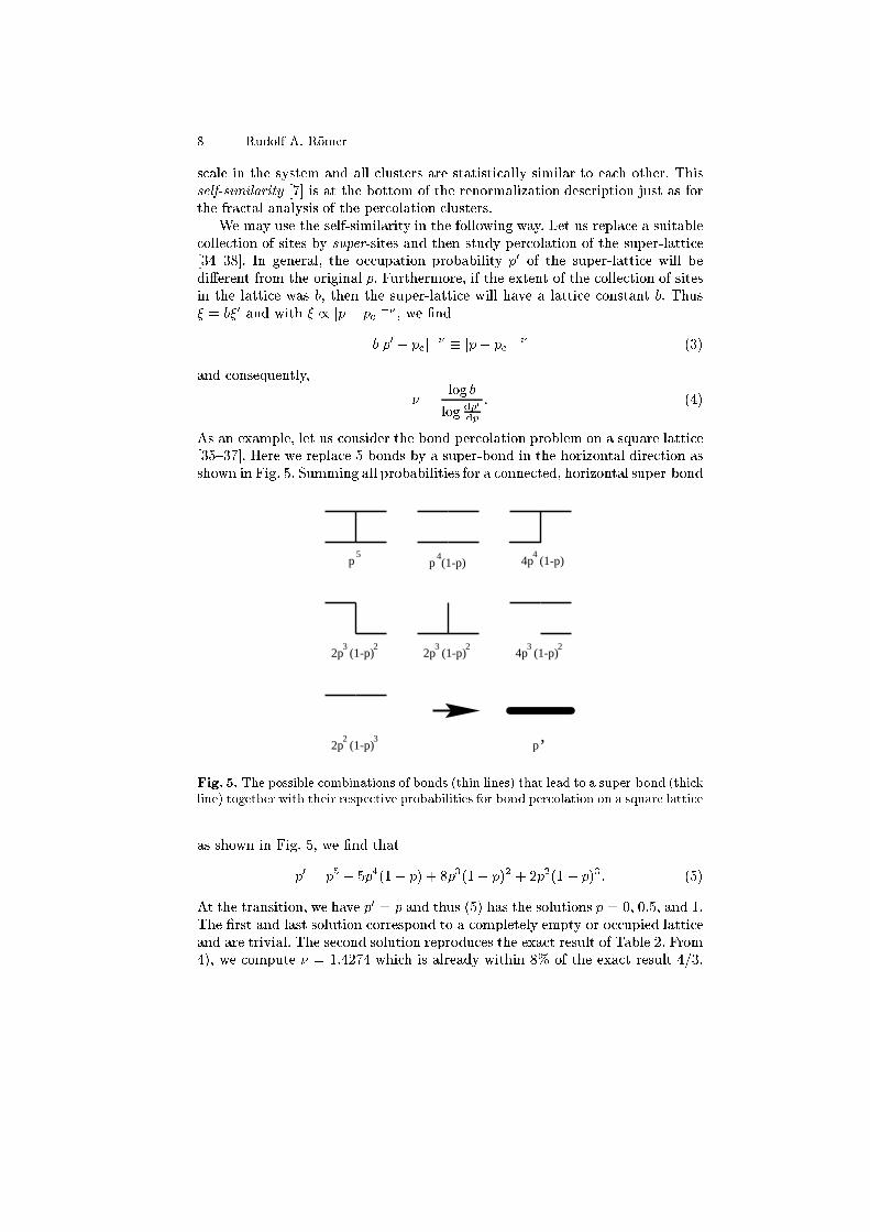
As an example, let us onsider the bond per olation problem on a square latti e

[35{37℄. Here we repla e 5 bonds by a super-bond in the horizontal dire tion as

shown in Fig. 5. Summing all probabilities for a onne ted, horizontal super-bond

4p (1-p)4p (1-p)

3 22p (1-p)

3 24p (1-p)

2 32p (1-p)

p5

3 22p (1-p)

4

,p

Fig. 5. The possible ombinations of bonds (thin lines) that lead to a super-bond (thi k

line) together with their respe tive probabilities for bond per olation on a square latti e

as shown in Fig. 5, we �nd that

p

0

= p

5

+ 5p

4

(1� p) + 8p

3

(1� p)

2

+ 2p

2

(1� p)

3

: (5)

At the transition, we have p

0

= p and thus (5) has the solutions p = 0, 0:5, and 1.

The �rst and last solution orrespond to a ompletely empty or o upied latti e

and are trivial. The se ond solution reprodu es the exa t result of Table 2. From

4), we ompute � = 1:4274 whi h is already within 8% of the exa t result 4=3.


Thus the real-spa e RG s heme gives very good approximations to the known

results. But beware, it may not always be that simple: the reader is en ouraged

to devise a similar RG s heme for site per olation on a square latti e.

3.2 Monte-Carlo RG

The s heme of the last se tion is approximate sin e it annot orre tly handle

situations like the one in Fig. 6. In order to improve, we an onstru t an RG

s heme that uses a larger olle tion of bonds. The total number of ( onne ted

and un onne ted) on�gurations in su h a olle tion of n bonds is 2

n

, putting

severe bounds on the pra ti ability of the approa h for analyti al ulations.

However, the task is ideally suited for omputers. On the CD a ompanying this

book, I in lude a set of Mathemati a routines that ompute the real-spa e RG

for a d = 2 triangular latti e.

Fig. 6. Although the original bonds (thin lines) are not onne ted, the RG pro edure

outlined in the text nevertheless leads to two onne ted horizontal super-bonds (thi k

lines)

4 The Quantum-Hall E�e t

In 1980, von Klitzing et al. [39℄ found that the Hall resistan e R

H

of MOSFETs

at strong magneti �eld B exhibits a step-like behavior whi h is a ompanied

with a simultaneously vanishing longitudinal resistan e R. This is in ontrast to

the lassi al Hall e�e t whi h gives a linear dependen e of R

H

on B. Even more

surprising, the values of R

H

at the transitions are given by universal onstants,

i.e.,

1

i

h

e

2

, where i is an integer.

Sin e its dis overy this so- alled integer quantum Hall e�e t (IQHE) was

studied extensively [40,41℄. Besides semi-phenomenologi al models simply as-

suming a lo alization-delo alization transition more general theories onsidered,

e.g., gauge invarian e [42℄, topologi al quantization [43℄, s attering [44℄ and �eld

theoreti al approa hes [45℄.

4.1 Basi s of the IQHE

A simple understanding of the IQHE an be gained by onsidering the Hamilto-

nian of a single ele tron in a magneti �eld,

H

0

=

1

2m

�

p+

e

A

�

2

=

�h!

2l

2

B

�

�

2

+ �

2

�

: (6)


where A denotes the ve tor potential and the Hamiltonian has been rewritten in

guiding enter oordinatesX = x��, Y = y�� and relative oordinates �, � [46℄.

Here, !

=

eB

m

is the frequen y of the lassi al y lotron motion and l

B

= (

�h

eB

)

1=2

is the radius of the y lotron motion. The spe trum of this Hamiltonian is simply

the harmoni os illator with E

n

=

�

n+

1

2

�

�h!

; n = 0, 1, : : :. These Landau

levels are in�nitely degenerate sin e the Hamiltonian no longer ontainsX and Y .

Thus the spe trum onsists of Æ-fun tion peaks as indi ated in Fig. 7. Introdu ing

disorder into the model by adding a smooth random potential V (r) in (6) results

in drift motion of the guiding enter

_

X =

i

�h

[H;X ℄ =

l

2

B

�h

�V

�y

;

_

Y =

i

�h

[H;Y ℄ = �

l

2

B

�h

�V

�x

: (7)

perpendi ular to the gradient of V (r) (see Fig. 8). Furthermore, the degenera y

of the Landau levels is lifted, the Æ-fun tion density of states broadens [40℄, giving

rise to a band-like stru ture as shown in Fig. 7. If the sample is penetrated by a

strong magneti �eld, the y lotron motion is mu h smaller than the potential

u tuations. Consequently, the ele tron motion an be separated into y lotron

motion and motion of the guiding enter along equipotential lines of the energy

lands ape.

��

��

��

��

σxx

σxy

��

eh

2

0 1

DO

S

νf

Fig. 7. Density of states (DOS), transversal and longitudinal ondu tivity as a fun tion

of E

F

or, equivalently, �lling fa tor �

f

or B

�1

[41℄. The peak in the middle of the band

represents one Æ-fun tion peak of the lean Landau model. Dark shaded regions of the

density of states orrespond to lo alized states. The thin dashed line (with non-zero

slope) for �

xy

indi ates the lassi al Hall result

The IQHE an then be understood as follows: assume that the enter of the

broadened Landau levels ontain extended states that an support transport,

whereas the other states are spatially lo alized and annot. This is similar to

the standard pi ture in the theory of Anderson lo alization [7,12℄. Changing the


Fermi energy E

F

or the �lling fa tor �

f

= 2�l

2

B

�

e

= 2��h�

e

=eB / E

F

, where �

e

denotes the ele tron density, we �rst have E

F

in the region of lo alized states

and both �

xx

and �

xy

are 0. When E

F

rea hes the region of extended states,

there is transport, �

xx

is �nite and �

xy

= e

2

=h. Next, E

F

again rea hes a region

of lo alized states and �

xx

drops ba k to 0 until we rea h the extended states in

the next Landau level.

This pi ture suggests the following e�e tive lassi al high-�eld model [47℄ of

the IQHE: Negle ting the y lotron motion (i.e., large B) and quantum e�e ts

(i.e., only one extended state) the lassi al ele tron transport with energy E

F

through the sample only depends on the \height" of the saddle points in the

potential energy lands ape V (r). One obtains a lassi al bond-per olation prob-

lem [5℄, in whi h saddle points are mapped onto bonds. A bond is onne ting

only when the potential of the orresponding saddle point equals the energy of

the ele tron E

F

. From per olation theory follows [5℄ that an in�nite system is

ondu ting only when E

F

= hV i. Using this model one ould already des ribe

the lo alization-delo alization transition and thus the quantized plateaus in re-

sistivity observed in IQHE [40℄. But for bond per olation the orrelation length

diverges at the transition with an exponent of � = 4=3 whi h is in ontrast to

the value found in the QH experiments.

4.2 RG for the Chalker-Coddington Network Model

The Chalker-Coddington (CC) network model improved the high-�eld model

by introdu ing quantum orre tions [48℄, namely tunneling and interferen e.

Tunneling o urs, in a semi lassi al view, when ele tron orbits ome lose enough

to ea h other and the ele tron y lotron motions overlap. This happens at the

saddle points, whi h now a t as quantum s atterers onne ting two in oming

with two outgoing hannels by a s attering matrix as shown in Fig. 8. Similar

to bond per olation a network an be onstru ted su h that the saddle points

are mapped onto bonds. While moving along an equipotential line an ele tron

a umulates a random phase whi h re e ts the disorder of V (r). Results for

this quantum per olation also show one extended state in the middle of the

Landau band. The riti al properties at the transition, espe ially the value of

the exponent � � 2:4 [49℄, agree with experiments [50,51℄.

As explained for the bond per olation problem we now apply the RG method

to the CC model. The RG stru ture whi h builds the new super-saddle points is

displayed in Fig. 9. It onsists of 5 saddle points drawn as bonds. The links (and

phase fa tors) onne ting the saddle points are indi ated by arrows pointing in

the dire tion of the ele tron motion due to the magneti �eld. Ea h saddle point

a ts as a s atterer onne ting the 2 in oming I

1;2

with the 2 outgoing hannels

O

1;2

�

O

1

O

2

�

=

�

t

i

r

i

r

i

�t

i

��

I

1

I

2

�

(8)

with re e tion oeÆ ients r

i

and transmission oeÆ ients t

i

, whi h are assumed

to be real numbers. The omplex phase fa tors enter later via the links between


Fig. 8. Left: S hemati plot of a smooth random potential V (r) with equipotential

lines at E = hV i indi ated in bla k. Right: Equipotential lines of the same potential

for E = hV i�E

max

=2, hV i, and hV i+E

max

=2 orresponding to long dashed, solid and

short dashed lines. Note the solid line per olating the system from top to bottom as

indi ated by the arrows

O1

I 1r

r

t

O2

I 2

−t φ

φ

φ

φ

Fig. 9. Left: A single saddle point ( ir le) onne ted to in oming and outgoing ur-

rents I

i

, O

i

via transmission and re e tion amplitudes t and r. Right: A network of 5

saddle points an be renormalized into a single super-saddle point by an RG approa h

very similar to the bond per olation problem of Se t. 3. The phases are s hemati ally

denoted by the �'s

the saddle points. By this de�nition { in luding the minus sign { the unitarity

onstraint t

2

i

+ r

2

i

= 1 is ful�lled a priori. The amplitude of transmission of the

in oming ele tron to another equipotential line and the amplitude of re e tion

and thus staying on the same equipotential line add up to unity { ele trons do

not get lost.

In order to obtain the s attering equation of the super-saddle point we now

need to onne t the 5 s attering equations a ording to Fig. 9. For ea h link the


amplitude of the in oming hannels is de�ned by the amplitude of the outgoing

hannel of the previous saddle point multiplied by the orresponding omplex

phase fa tor e

i�

k

. This results in a system of 5 matrix equations, whi h has to

be solved. One obtains an RG equation for the transmission oeÆ ient t

0

of the

super-saddle point [52℄ analogously to Eq. (5),

t

0

=

t

15

(r

234

e

i�

2

� 1) + t

24

e

i(�

3

+�

4

)

(r

135

e

�i�

1

� 1) + t

3

(t

25

e

i�

3

+ t

14

e

i�

4

)

(r

3

� r

24

e

i�

2

)(r

3

� r

15

e

i�

1

) + (t

3

� t

45

e

i�

4

)(t

3

� t

12

e

i�

3

)

(9)

depending on the produ ts t

i:::j

= t

i

� : : : �t

j

, r

i:::j

= r

i

� : : : �r

j

of transmission and

re e tion oeÆ ients t

i

and r

i

of the i = 1; : : : ; 5 saddle points and the 4 random

phases �

k

a umulated along equipotentials in the original latti e. For further

algebrai simpli� ation one an apply a useful transformation of the amplitudes

t

i

= (e

z

i

+1)

�1=2

and r

i

= (e

�z

i

+1)

�1=2

to heights z

i

relative to heights V

i

of the

saddle points. The ondu tan e G is onne ted to the transmission oeÆ ient t

by G = jtj

2

e

2

=h [53℄.

4.3 Condu tan e Distributions at the QH Transition

For the numeri al determination of the ondu tan e distribution, we �rst hoose

an initial probability distribution P

0

of transmission oeÆ ients t. The distribu-

tion is dis retized in at least 1000 bins. Thus the bin width is typi ally 0:001e=

p

h

for the interval t 2 [0; e=

p

h℄.

Using the initial distribution P

0

(t), we now randomly sele t many di�erent

transmission oeÆ ients and insert them into the RG equation (9). Further-

more, the phases �

j

, j = 1; : : : 4 are also hosen randomly, but a ording to a

uniform distribution �

j

2 [0; 2�℄. By this method at least 10

7

super-transmission

oeÆ ients t

0

are al ulated and their distribution P

1

(t

0

) is stored. Next, P

1

is

averaged using a Savitzky-Golay smoothing �lter [54℄ in order to de rease sta-

tisti al u tuations. This pro ess is then repeated using P

1

as the new initial

distribution.

The iteration pro ess is stopped when the distribution P

i

is no longer distin-

guishable from its prede essor P

i�1

and we have rea hed the desired �xed-point

(FP) distribution P

(t). However, due to numeri al instabilities, small deviations

from symmetry add up su h that typi ally after 15{20 iterations the distributions

be ome unstable and onverge towards the lassi al FPs of no transmission or

omplete transmission similar to the lassi al per olation ase. Figure 10 shows

this behavior for one of the RG iterations. The FP distribution P

(G) shows a

at minimum around G = 0:5e

2

=h and sharp peaks at G = 0 and G = e

2

=h.

It is symmetri with hGi = 0:498e

2

=h. This is in agreement with previous the-

oreti al [56,57℄ and experimental [58℄ results whereas our results ontain mu h

less statisti al u tuations. Furthermore we determine moments h(G�hGi)

m

i of

the FP distribution P

(G). As shown in Fig. 10 for small moments up to m = 6

our results agree with the work of Wang et al. [55℄, who omputed moments

m � 8:5. But more interesting is the fa t that the obtained moments of the FP

distribution an hardly be distinguished from the moments of a simple onstant


0 0.2 0.4 0.6 0.8 1G

0.5

1

1.5

2

P(G

)

2 4 6 8 10 20 30m

−10

−8

−6

−4

−2

0

log 10

<(G

−<

G>

)m>

Fig. 10. Condu tan e distribution at a QH plateau-to-plateau transition. The squares

orrespond to the �xed-point distribution, dashed and dot-dashed lines to the initial

distribution and an unstable distribution, respe tively. The solid line indi ates a �t of

the FP distribution P

(t) by three Gaussians. Inset: Moments of the FP distribution

P

(G). The dashed lines indi ate various predi tions based on extrapolations of results

for small m [55℄. The dotted line denotes the moments of a onstant distribution

distribution thus indi ating the in uen e of the broad at minimum of the FP

distribution around G = 0:5e

2

=h.

For the determination of the riti al exponent, we next perturb the FP dis-

tribution slightly, i.e., we onstru t a distribution with shifted average G

0

. Then

we perform an RG iteration and ompute the new average G

1

of P

1

(G). Tra ing

the shift of the perturbed average G

n

for several initial shifts G

0

, we expe t to

�nd a linear dependen e of G

n

on G

0

for ea h iteration step n. The riti al ex-

ponent is then related to the slope dG

n

=dG

0

[59℄. Figure 11 shows the resulting

� in dependen e on the iteration step and thus system size. The urve onverges

lose to � � 2:4, i.e. the value obtained by Lee et al. [49℄. Note that the \sys-

tem size" is more properly alled a system magni� ation, sin e we start the RG

iteration with an FP distribution valid for an in�nite system and then magnify

the system in the ourse of the iteration by a fa tor 2

n

.

5 Summary and Con lusions

The per olation model represents the perhaps simplest example of a system

exhibiting omplex behavior although its onstituents { the sites and bonds {

are hosen ompletely un orrelated. Of ourse, the omplexity enters through the


4 16 32 64 128 2562

n

2.2

2.4

2.6

2.8

3.0

3.2

ν

0 0.05 0.1

<G>−G0

0.00

0.10

0.20

<G>−

Gn

Fig. 11. Criti al exponent � as a fun tion of magni� ation fa tor 2

n

for RG step n.

The dashed line shows the expe ted result � = 2:39. Inset: The shift of the average G

n

of P (G) is linear in G

0

. The dashed lines indi ate linear �ts to the data

onne tivity requirement for per olating lusters. I have reviewed several numer-

i al algorithms for quantitatively measuring various aspe ts of the per olation

problem. The spe i� hoi e re e ts purely my personal preferen es and I am

happy to note that other algorithms su h as breadth- and depth-�rst algorithms

[60℄ have been introdu ed by P. Grassberger in his ontribution [61℄.

The real-spa e RG provides an instru tive use of the underlying self-similarity

of the per olation model at the transition. Furthermore, it an be used to study

very large e�e tive system sizes. This is needed in many appli ations. As an

example, I brie y reviewed and studied the QH transition and omputed on-

du tan e distributions, moments and the riti al exponent. These results an be

ompared to experimental measurements and shown to be in quite good agree-

ment.

A knowledgements

The author thanks Phillip Cain, Ralf Hamba h, Mikhail E. Raikh, and Andreas

R�osler for many helpful dis ussions. This work was supported by the NSF-DAAD

ollaborative resear h grant INT-9815194, the DFG within SFB 393 and the

DFG-S hwerpunktprogramm \Quanten-Hall-Systeme".


Referen es

1. We note that the WEH-Ferienkurs, following whi h this arti le has been prepared,

took pla e during early fall.

2. S.R. Broadbent, J.M. Hammersley: Pro . Camb. Philos. So . 53, 629 (1957)

3. J.M. Hammersley: Pro . Camb. Philos. So . 53, 642 (1957)

4. J.M. Hammersley: Ann. Math. Statist. 28, 790 (1957)

5. D. Stau�er, A. Aharony: Perkolationstheorie (VCH, Weinheim 1995)

6. For any �nite latti e, \in�nite" means a luster that rea hes from top to bottom

and/or left to right through the latti e.

7. M. S hreiber, F. Milde (this volume).

8. K. Binder: Rep. Prog. Phys. 60, 487 (1997)

9. G. Grimmett: Per olation (Springer, Berlin 1989)

10. A. Bunde, S. Havlin (Eds.): Per olation and Disordered Systems: Theory and Ap-

pli ations (North-Holland, Amsterdam 1999)

11. T. Vojta, (this volume).

12. B. Kramer, (this volume).

13. U. Grimm, (this volume).

14. K. S henk, B. Drossel, F. S hwabl, (this volume).

15. J. Voit: The Statisti al Me hani s of Capital Markets (Springer, Heidelberg 2001)

16. J. Goldenberg, B. Libai, S. Solomon, N. Jan, D. Stau�er: Marketing Per olation

(2000). Cond-mat/9905426

17. http://de.arXiv.org/, 1993{2000

18. J. Hoshen, R. Kopelman: Phys. Rev. B 14, 3438 (1976)

19. C. Adami: (1997),

http://www.krl. alte h.edu/~adami/CD1/Per olation/per olation.html,

likely to hange without prior noti e

20. P. Leath: Phys. Rev. B 14, 5056 (1976)

21. W. Kinzel, G. Reents: Physi s by Computer (Springer, Berlin 1998)

22. W. Kinzel, G. Reents: (1999),

http://wptx15.physik.uni-wuerzburg.de/TP3/applet_java/per gr.html,

likely to hange without prior noti e

23. R.F. Voss: J. Phys. A: Math. Gen. 17(7), L373 (1984)

24. R.M. Zi�, P.T. Cummings, G. Stell: J. Phys. A: Math. Gen. 17, 3009 (1984)

25. M. Rosso, J.F. Gouyet, B. Sapoval: Phys. Rev. B 32, 6053 (1985)

26. R.M. Zi�, B. Sapoval: J. Phys. A: Math. Gen. 19, L1169 (1986)

27. Alas, this intuitively onvin ing argument is not stri tly true: The per olation

frontier is a fra tal and as su h s ales / L

1:75

[23℄. On the other hand, it is not

the random number generation for L

2

sites in the Hoshen-Kopelman algorithm but

rather the numeri al determination of the per olating lusters whi h is numeri ally

hallenging.

28. P.N. Suding, R.M. Zi�: Phys. Rev. E 60, 275 (1999)

29. M.F. Sykes, J.W. Essam: Phys. Rev. Lett. 10, 3 (1963)

30. R.M. Zi�, P.N. Suding: J. Phys. A: Math. Gen. 30, 5351 (1997)

31. C.D. Lorenz, R.M. Zi�: Phys. Rev. B 57, 230 (1998)

32. P. Kleban, R.M. Zi�: Phys. Rev. B 57, R8075 (1998)

33. M.E.J. Newman, R.M. Zi�: (2000). Cond-mat/0005264

34. A.B. Harris, T.C. Lubensky, W.K. Hol omb, C. Dasgupta: Phys. Rev. Lett. 35,

327 (1975)


35. P.J. Reynolds, W. Klein, H.E. Stanley: J. Phys. C: Solid State Phys. 10, L167

(1977)

36. J. Bernas oni: Phys. Rev. B 18, 2185 (1978)

37. P.J. Reynolds, H.E. Stanley, W. Klein: Phys. Rev. B 21, 1223 (1980)

38. P.D. Es hba h, D. Stau�er, H. Herrmann: Phys. Rev. B 23, 422 (1981)

39. K.v. Klitzing, G. Dorda, M. Pepper: Phys. Rev. Lett. 45, 494 (1980)

40. M. Janssen, O. Viehweger, U. Fastenrath, J. Hajdu: Introdu tion to the Theory of

the Integer Quantum Hall e�e t (VCH, Weinheim 1994)

41. T. Chakraborty, P. Pietil�anen: The Quantum Hall e�e ts (Springer, Berlin 1995)

42. R.B. Laughlin: Phys. Rev. B 23, 5632 (1981)

43. D.J. Thouless, M. Kohmoto, M.P. Nightingale, M. den Nijs: Phys. Rev. Lett. 49,

405 (1982)

44. R.E. Prange: Phys. Rev. B 23, 4802 (1981)

45. A.M.M. Pruisken: Nu l. Phys. B 235, 277 (1984)

46. D.L. Landau: Z. Phys. 64, 629 (1930)

47. S.V. Iordanskii: Solid State Commun. 43, 1 (1982)

48. J.T. Chalker, P.D. Coddington: J. Phys.: Condens. Matter 21, 2665 (1988)

49. D.H. Lee, Z. Wang, S. Kivelson: Phys. Rev. Lett. 70, 4130 (1993)

50. S. Ko h, R.J. Haug, K. v. Klitzing, K. Ploog: Phys. Rev. B 43, 6828 (1991)

51. R.T.F. van S haijk, A. de Visser, S.M. Olsthoorn, H.P. Wei, A.M.M. Pruisken:

Phys. Rev. Lett. 84, 1567 (2000)

52. A.G. Galstyan, M.E. Raikh: Phys. Rev. B 56, 1422 (1997)

53. M. B�uttiker, Y. Imry, R. Landauer, S. Pinhas: Phys. Rev. B 31, 6207 (1985)

54. W.H. Press, B.P. Flannery, S.A. Teukolsky, W.T. Vetterling: Numeri al Re ipes

in FORTRAN , 2nd edn. (Cambridge University Press, Cambridge 1992)

55. Z. Wang, B. Jovanovi , D.H. Lee: Phys. Rev. Lett. 77, 4426 (1996)

56. A. Weymer, M. Janssen: Ann. Phys. (Leipzig) 7, 159 (1998). Cond-mat/9805063

57. Y. Avishai, Y. Band, D. Brown: Phys. Rev. B 60, 8992 (1999)

58. D.H. Cobden, E. Kogan: Phys. Rev. B 54, R17 316 (1996)

59. P. Cain, R.A. R�omer, M.E. Raikh, M. S hreiber: Lo alization-Delo alization quan-

tum Hall transition in the present of a quen hed disorder (2001).

60. A. Aho, J.E. Hop roft, J.D. Ullman: Data Stru tures and Algorithms (Addison-

Wesley, New York 1983)

61. P. Grassberger, (this volume).

ercolation, p - technische universität chemnitz · ercolation p and tum-hall quan ransition t 3...

Documents