ERD

C/EL

TR-

12-6

Dredging Operations and Environmental Research Program

Incorporation of Chemical Contaminants into the Combined ICM/SEDZLJ Models

Envi

ronm

enta

l Lab

orat

ory

Carl F. Cerco March 2012

Approved for public release; distribution is unlimited.

Dredging Operations and Environmental Research

ERDC/EL TR-12-6 March 2012

Incorporation of Chemical Contaminants into the Combined ICM/SEDZLJ Models

Carl F. Cerco Environmental Laboratory U.S. Army Engineer Research and Development Center 3909 Halls Ferry Road Vicksburg, MS 39180

Final report Approved for public release; distribution is unlimited.

ERDC/EL TR-12-6 ii

Abstract

This report describes two tasks. The first is the conversion of the combined ICM/SEDZLJ computer codes to parallel operation. The conversion results in order-of-magnitude speed-up of the combined codes with no adverse effects on the computation. Results from parallel operation are identical to serial operation for up to 128 processors.

The second task is the incorporation of an initial toxics code into the combined ICM/SEDZLJ codes. Two toxicants are considered. The first partitions to clay/silt particles in the water and bed sediments. The second partitions to particulate organic carbon. Treatment of the new variables in the water column is analogous to the three-dimensional, finite-volume approach used for the other ICM state variables. In the bed, toxics are considered to occupy a single well-mixed layer roughly 10 cm in thickness. This approach is adopted from the ICM sediment diagenesis model. Particle deposition and erosion and the resulting effects on bed thickness are taken from SEDZLJ. This framework forms the initial basis for a unified model of the aquatic carbon cycle, of particulate transport, and of toxicant processes.

DISCLAIMER: The contents of this report are not to be used for advertising, publication, or promotional purposes. Citation of trade names does not constitute an official endorsement or approval of the use of such commercial products. All product names and trademarks cited are the property of their respective owners. The findings of this report are not to be construed as an official Department of the Army position unless so designated by other authorized documents. DESTROY THIS REPORT WHEN NO LONGER NEEDED. DO NOT RETURN IT TO THE ORIGINATOR.

ERDC/EL TR-12-6 iii

Contents Figures and Tables ................................................................................................................................. iv

Preface .................................................................................................................................................... vi

1 Introduction ..................................................................................................................................... 1

2 Conversion from Serial to Parallel Mode ..................................................................................... 3

3 Toxics Model Formulation ............................................................................................................. 7

Introduction .............................................................................................................................. 7 Toxics in the water column....................................................................................................... 7

Internal sources and sinks .......................................................................................................... 8 Particulate and dissolved fractions ........................................................................................... 10

Toxics in the bed ..................................................................................................................... 11 Deposition and erosion .............................................................................................................. 12 Bed thickness ............................................................................................................................. 13

4 Basic Performance Tests ............................................................................................................. 15

Mass conservation ................................................................................................................. 15 Model time-step ...................................................................................................................... 17 Settling velocity ...................................................................................................................... 18 Transport ................................................................................................................................. 18 Bed armoring .......................................................................................................................... 20 Continuous erosion ................................................................................................................ 23 Continuous deposition ........................................................................................................... 23

5 Summary and Conclusions .......................................................................................................... 27

References ............................................................................................................................................ 29

Report Documentation Page

ERDC/EL TR-12-6 iv

Figures and Tables

Figures

Figure 1. Computation of clay in the surface layer of Lake George for 1, 4, and 16 processors. .............. 4

Figure 2. Computation of deposition from water to bottom sediments of Lake George for 1, 4, and 16 processors. ............................................................................................................................ 5

Figure 3. Computation of erosion from bottom sediments to water column of Lake George for 1, 4, and 16 processors. ...................................................................................................................... 5

Figure 4. Computation of sediment bed mass of Lake George for 1, 4, and 16 processors. ............ 6

Figure 5. Computation time versus number of processors. Results are for a three-year simulation of Lake George (563 surface cells x 2 deep) on a Cray XE6 rated at 194.2 peak TFLOPS. ....................................................................................................................................................... 6

Figure 6. Schematic of toxics model in the water column. .................................................................... 9

Figure 7. Schematic of toxics model in the bed. Note that the toxics bed consists of a single well-mixed layer, initially 10 cm thick, in contrast to the SEDZLJ bed, which includes multiple layers. Deposition, erosion, and bed thickness are shared by both models. ...................... 11

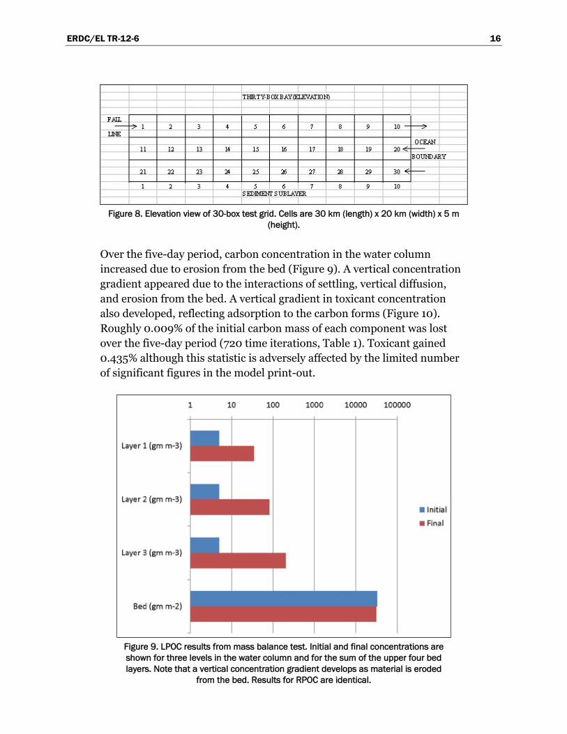
Figure 8. Elevation view of 30-box test grid. Cells are 30 km (length) x 20 km (width) x 5 m (height). ..................................................................................................................................................... 16

Figure 9. LPOC results from mass balance test. Initial and final concentrations are shown for three levels in the water column and for the sum of the upper four bed layers. Note that a vertical concentration gradient develops as material is eroded from the bed. Results for RPOC are identical. ............................................................................................................... 16

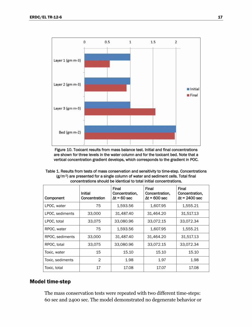
Figure 10. Toxicant results from mass balance test. Initial and final concentrations are shown for three levels in the water column and for the toxicant bed. Note that a vertical concentration gradient develops which corresponds to the gradient in POC. ................................... 17

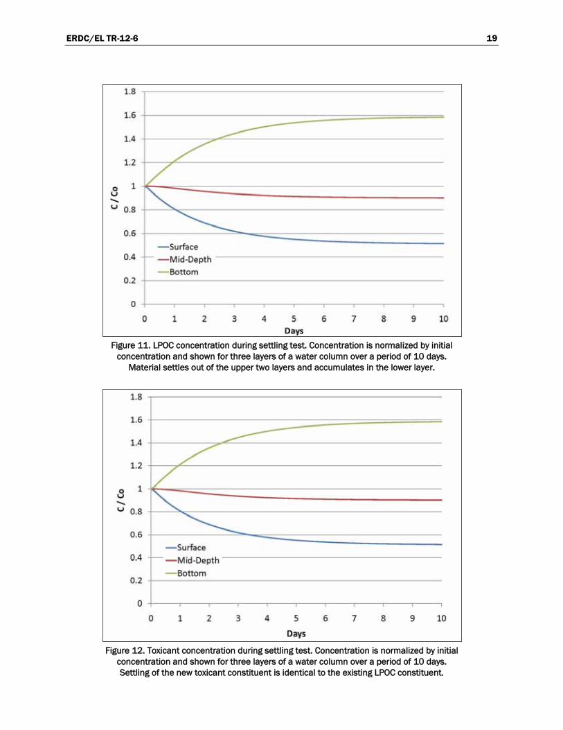
Figure 11. LPOC concentration during settling test. Concentration is normalized by initial concentration and shown for three layers of a water column over a period of 10 days. Material settles out of the upper two layers and accumulates in the lower layer. ............................. 19

Figure 12. Toxicant concentration during settling test. Concentration is normalized by initial concentration and shown for three layers of a water column over a period of 10 days. Settling of the new toxicant constituent is identical to the existing LPOC constituent. ......................... 19

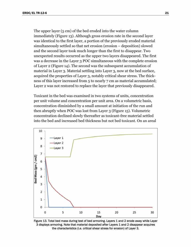
Figure 13. Total bed mass during test of bed armoring. Layers 1 and 2 erode away while Layer 3 displays armoring. Note that material deposited after Layers 1 and 2 disappear acquires the characteristics (i.e. critical shear stress for erosion) of Layer 3. ................................... 21

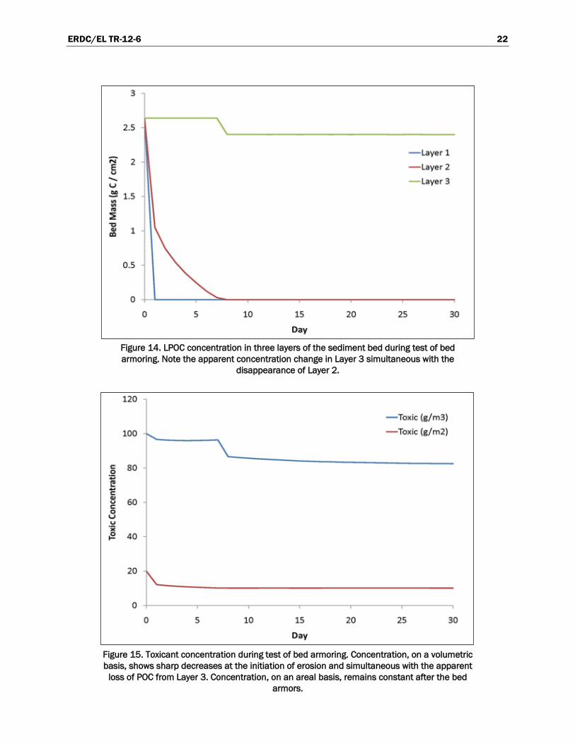
Figure 14. LPOC concentration in three layers of the sediment bed during test of bed armoring. Note the apparent concentration change in Layer 3 simultaneous with the disappearance of Layer 2. ....................................................................................................................... 22

Figure 15. Toxicant concentration during test of bed armoring. Concentration, on a volumetric basis, shows sharp decreases at the initiation of erosion and simultaneous with the apparent loss of POC from Layer 3. Concentration, on an areal basis, remains constant after the bed armors. ............................................................................................................... 22

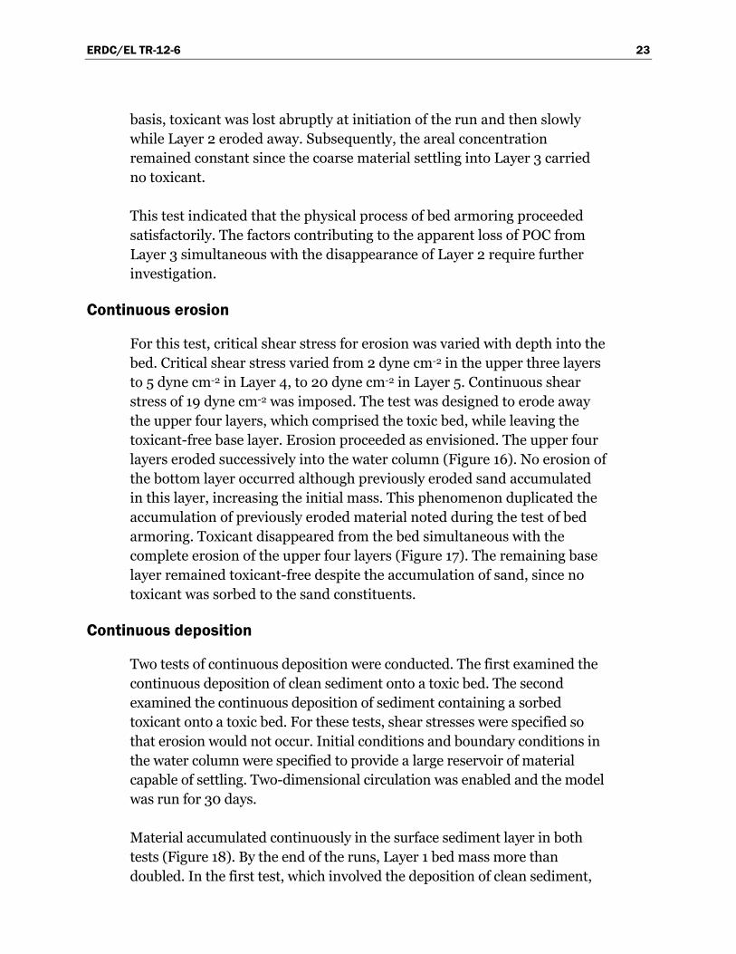
Figure 16. Bed mass during test of continuous erosion. The upper four bed layers erode immediately. The bottom layer resists erosion but acquires material through settling. .................... 24

ERDC/EL TR-12-6 v

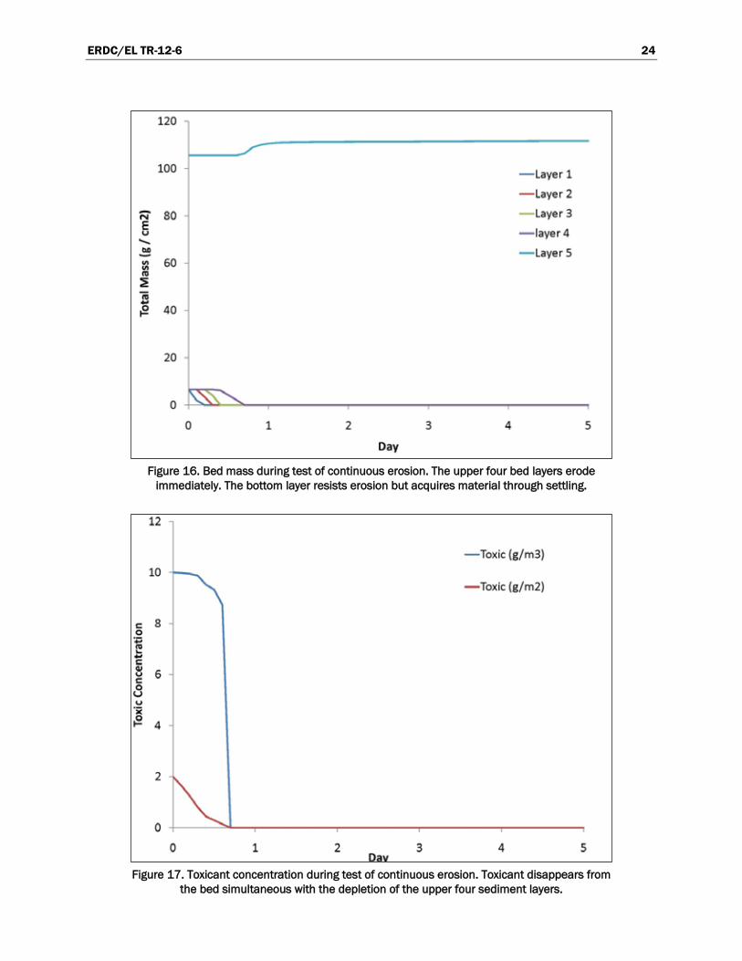
Figure 17. Toxicant concentration during test of continuous erosion. Toxicant disappears from the bed simultaneous with the depletion of the upper four sediment layers. .......................... 24

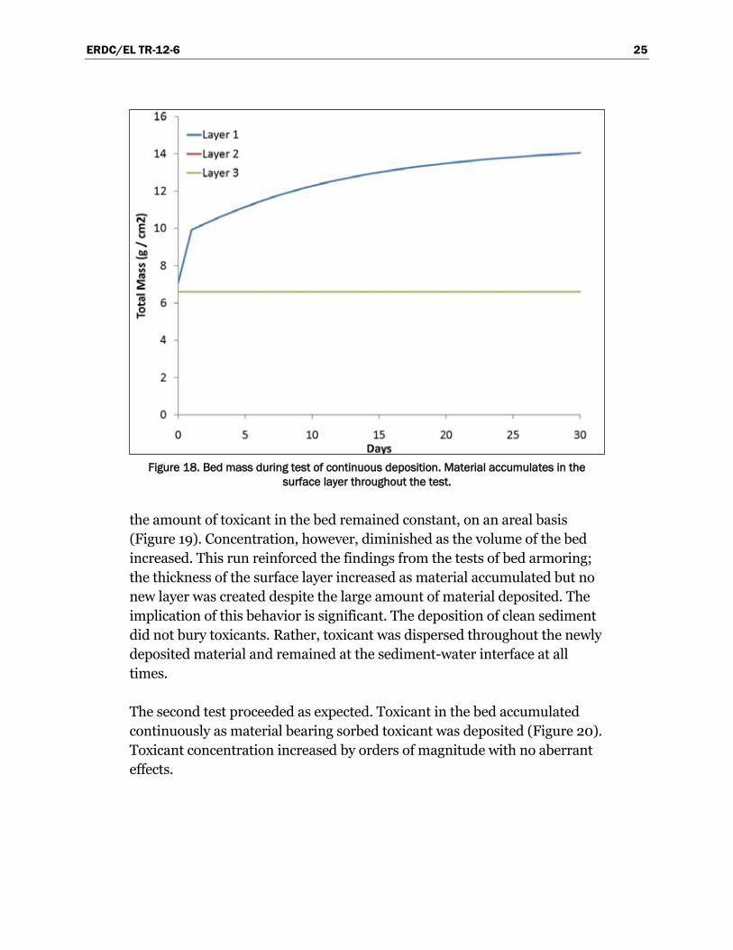
Figure 18. Bed mass during test of continuous deposition. Material accumulates in the surface layer throughout the test............................................................................................................ 25

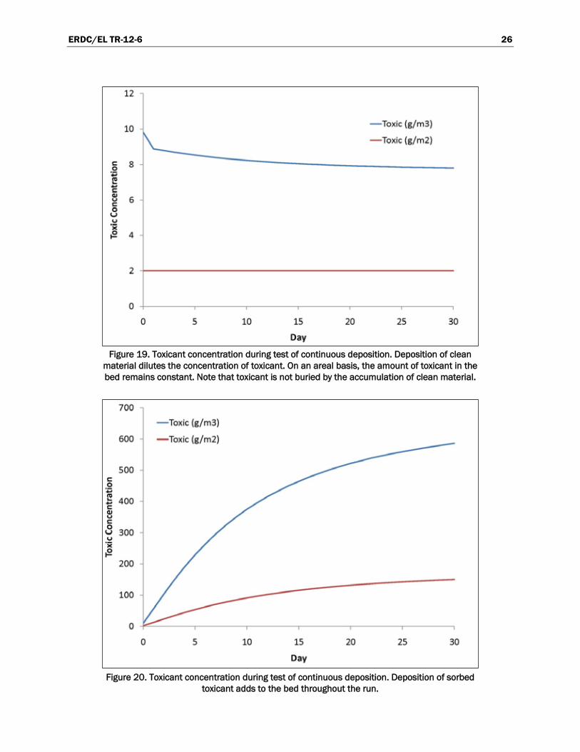
Figure 19. Toxicant concentration during test of continuous deposition. Deposition of clean material dilutes the concentration of toxicant. On an areal basis, the amount of toxicant in the bed remains constant. Note that toxicant is not buried by the accumulation of clean material. ...................................................................................................................................... 26

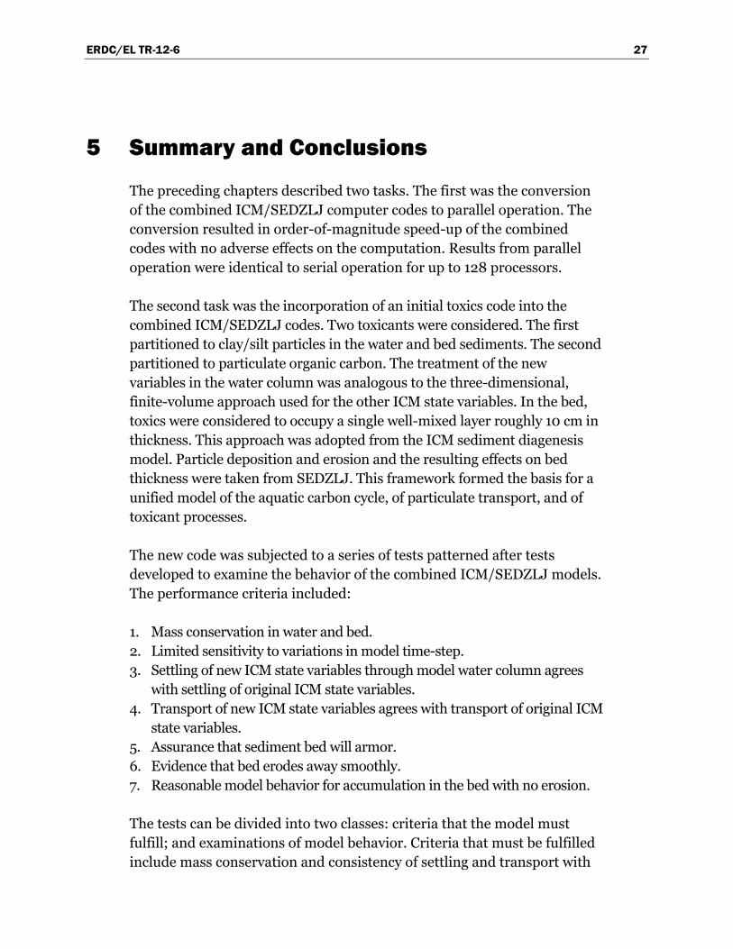
Figure 20. Toxicant concentration during test of continuous deposition. Deposition of sorbed toxicant adds to the bed throughout the run. ........................................................................... 26

Tables

Table 1. Results from tests of mass conservation and sensitivity to time-step. Concentrations (g/m-2) are presented for a single column of water and sediment cells. Total final concentrations should be identical to total initial concentrations. .................................... 17

Table 2. Results from transport test for a dissolved toxicant. Concentrations are presented for each cell in the 30-box test grid (Figure 8) after a 30-day model run. Transport of the new toxicant constituent is identical to the existing salinity constituent. ........................................... 20

Table 3. Results from transport test for a particulate toxicant. Concentrations are presented for each cell in the 30-box test grid (Figure 8) after a 30-day model run. Transport of the new toxicant constituent is identical to the existing LPOC constituent. .................. 20

ERDC/EL TR-12-6 vi

Preface

This work described in this report was funded by the Dredging Operations and Environmental Research (DOER) Program, Dr. Todd Bridges, Program Manager. The work was conducted under the supervision of Warren Lorentz, Chief, Environmental Processes and Engineering Division, Environmental Laboratory (EL), U.S. Army Engineer Research and Development Center (ERDC), Vicksburg, MS.

This report was prepared by Dr. Carl F. Cerco of the Water Quality and Contaminant Modeling Branch, EL, ERDC. At the time of publication of this report, Dr. Beth Fleming was Director of EL.

COL Kevin J. Wilson was Commander of ERDC. Dr. Jeffery P. Holland was Director.

ERDC/EL TR-12-6 1

1 Introduction

This report describes work completed in a Dredging Operations and Environmental Research (DOER) Program work unit entitled “High-Fidelity Contaminant Fate and Transport Model.” The goal of the project is to produce a high-fidelity contaminant fate and transport model within the framework of the CE-QUAL-ICM (or simply ICM) finite-volume water quality model (Cerco and Cole 1994). A previous report (Cerco, in prepara-tion) describes the merger of the SEDZLJ sediment transport model (Jones and Lick 2001) with ICM. Merging of the two models is necessary because contaminants commonly partition to sediments of various compositions and are therefore transported along with the sediments. The coupling of SEDZLJ with ICM takes advantage of the detailed ICM representation of the aquatic carbon cycle in the water column and bed sediments, which is necessary since hydrophobic contaminants display a strong tendency to adhere to organic carbon particles.

The preceding report noted that coupling with a mechanistic sediment transport model forced a reduction in the ICM integration time-step from minutes to seconds. The shorter time-step was necessitated by rapid settling of coarse particles through the water column and by the detailed computa-tions of sediment deposition and resuspension. As a consequence, computa-tion time increased by an order of magnitude over the time required by ICM for eutrophication simulations without sediment transport. The first portion of this publication describes efforts to convert the combined models from serial to parallel computation mode, in order to reduce computational demands to practical levels.

The second portion of this publication describes the formulation of an initial toxicant model, which is incorporated into ICM and operated in tandem with the SEDZLJ deposition and resuspension algorithms. Two toxicants are represented in the water column. One partitions to particulate organic carbon forms, the other partitions to fine inorganic sediment particles. Both toxicants exchange with a well-mixed sediment bed via diffusion of the dissolved fraction and deposition/resuspension of the particulate fraction.

ERDC/EL TR-12-6 2

The toxicant model is subjected to a series of performance tests patterned after tests devised for the coupled ICM/SEDZLJ models. These tests include:

1. Mass conservation in water and bed. 2. Limited sensitivity to variations in model time-step. 3. Determining whether settling of new ICM state variables through the

model water column agrees with settling of original ICM state variables. 4. Determining whether transport of new ICM state variables agrees with

transport of original ICM state variables. 5. Determining whether sediment bed will armor. 6. Determining whether bed erodes away smoothly. 7. Determining whether model behaves reasonably for accumulation in the

bed with no erosion.

ERDC/EL TR-12-6 3

2 Conversion from Serial to Parallel Mode

Characteristics of the combined ICM and SEDZLJ codes were explored through application to a prototype system, Lake George, Florida (Cerco, in preparation). Application of the sediment transport algorithms required reduction of the ICM integration time-step to 60 sec versus 15 min for application of the ICM eutrophication algorithms alone. As a result of the reduced time-step and additional computational demands imposed by the SEDZLJ bed model, the computation time of the combined ICM/SEDZLJ models increased tremendously over the basic eutrophication model. A three-year simulation of Lake George eutrophication consumed 4 hr on a desktop PC while a three-year simulation of suspended solids, using SEDZLJ, consumed four days. Although computation time would be less on a faster computer, the practical application of the combined codes was severely limited.

The computational demand of the combined codes was reduced through conversion from serial (one CPU) to parallel (multiple CPU’s) operational mode. The parallelization employed the technique known as “domain decomposition” in which the model computational grid (domain) is broken into a number of smaller grids (domains). Computations on each individual grid are conducted by a separate processor, thereby greatly reducing computational time compared to execution of the entire grid on a single processor. The decomposition requires pre- and post-processing steps. In the pre-processing step, the model input files are separated into individual files for each sub-grid. In the post-processing step, outputs from the sub-grids are assembled into a single output file identical in format to the output file from a serial run. Domain decomposition was previously applied to the ICM eutrophication code (Chippada et al. 1998, Noel et al. 2000). The procedure conducted for this study consisted of the following tasks:

• Modify the model preprocessor to accommodate the new SEDZLJ input decks.

• Modify the model postprocessor to accommodate outputs from the SEDZLJ algorithms.

• Validate the parallel operation of the new ICM sediment constituents.

ERDC/EL TR-12-6 4

• Ensure model results are identical when operated in serial or parallel mode.

• Test model performance with the computational domain divided into an increasing number of sub-domains.

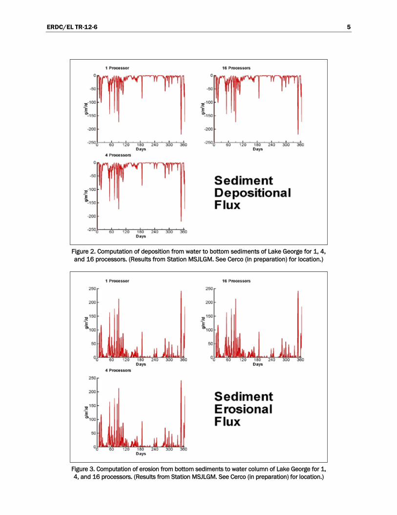
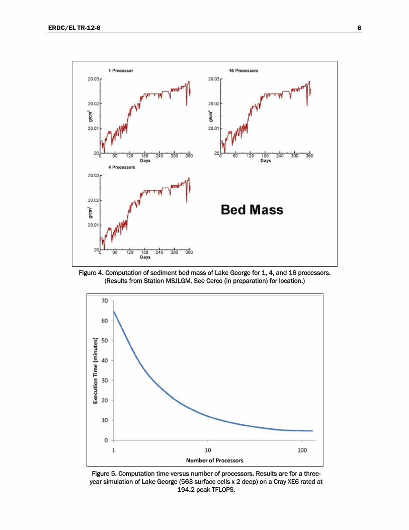
Tests conducted following parallelization indicated results from model operation in parallel mode were identical to operation in serial mode (Figures 1–4). Performance tests indicated computational time could be readily reduced by an order of magnitude (Figure 5). For Lake George, 32 processors provided order-of-magnitude speed-up. The marginal benefit of adding processors beyond this number was small, as the benefit gained by more processors was overtaken by the increased time necessary to communicate between processors. The optimal number of processors and computational benefits depends on the number of grid cells in the computational domain and on additional factors and will differ for systems other than Lake George. However, the parallel algorithms and processors and the availability of order-of-magnitude speed-up will transfer to alternate applications.

Figure 1. Computation of clay in the surface layer of Lake George for 1, 4, and 16 processors.

(Results from Station MSJLGM. See Cerco (in preparation) for location.)

ERDC/EL TR-12-6 5

Figure 2. Computation of deposition from water to bottom sediments of Lake George for 1, 4, and 16 processors. (Results from Station MSJLGM. See Cerco (in preparation) for location.)

Figure 3. Computation of erosion from bottom sediments to water column of Lake George for 1, 4, and 16 processors. (Results from Station MSJLGM. See Cerco (in preparation) for location.)

ERDC/EL TR-12-6 6

Figure 4. Computation of sediment bed mass of Lake George for 1, 4, and 16 processors.

(Results from Station MSJLGM. See Cerco (in preparation) for location.)

Figure 5. Computation time versus number of processors. Results are for a three-

year simulation of Lake George (563 surface cells x 2 deep) on a Cray XE6 rated at 194.2 peak TFLOPS.

ERDC/EL TR-12-6 7

3 Toxics Model Formulation Introduction

A variety of toxics models are available within (Boyer et al. 1994) and outside (Tetra Tech 2007; U.S. Environmental Protection Agency (USEPA) 1987) the Corps. Model representations of hydrophobic contaminants in the water column are usually similar with regard to processes and formulations, but representations of the sediment bed vary widely. At one extreme, bed models resolve the bed into multiple vertical layers, provide detailed representation of erosion and deposition, and compute processes on the time scale of seconds (Tetra Tech 2007). At the other extreme, bed sedi-ments are represented as well mixed, erosion and deposition are considered as long-term average processes, and time scales extend to decades or centuries (Boyer et al. 1994). This study calls for the adaptation, to the greatest extent possible, of one or more existing Corps frameworks.

The current effort begins with a basic toxics model, which is modified from one originally developed for Lake Washington, Washington (Cerco et al. 2004). The major modification substitutes dynamic sediment deposition and resuspension, calculated via SEDZLJ, for the long-term average deposi-tion used in Lake Washington. The intention is to test basic formulation and coding before moving to a more advanced, complex representation. Two toxicants are added to the ICM parameter suite. The first partitions to fine sediment particles such as clay. The second partitions to particulate organic carbon forms. Formulations for the two toxicants are identical except for the nature of solids to which they partition.

A major objective of the modeling is to represent the partitioning of hydro-phobic contaminants directly to particulate organic carbon. The partitioning of the second contaminant mentioned above fulfills the original intention. Partitioning to fine, inorganic sediments adds model flexibility. If desired, the first toxicant can be configured to resemble conventional contaminant modeling in which particulate organic carbon is represented as a fixed fraction of fine sediments.

Toxics in the water column

The foundation of CE-QUAL-ICM is the solution to the three-dimensional mass-conservation equation for a control volume. Control volumes

ERDC/EL TR-12-6 8

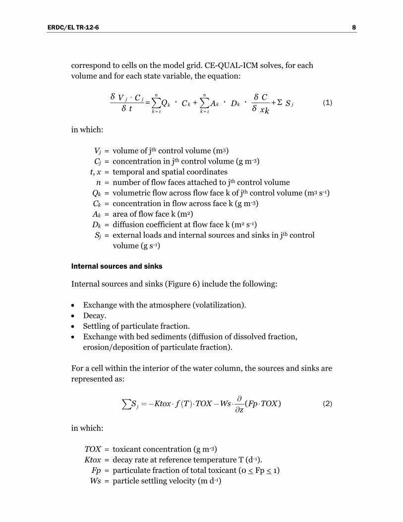
correspond to cells on the model grid. CE-QUAL-ICM solves, for each volume and for each state variable, the equation:

Σn n

j jk kk jk

k = 1 k = 1

δ δ CV C = + + Q C SA Dδ t δ xk

(1)

in which:

Vj = volume of jth control volume (m3) Cj = concentration in jth control volume (g m-3) t, x = temporal and spatial coordinates n = number of flow faces attached to jth control volume Qk = volumetric flow across flow face k of jth control volume (m3 s-1) Ck = concentration in flow across face k (g m-3) Ak = area of flow face k (m2) Dk = diffusion coefficient at flow face k (m2 s-1) Sj = external loads and internal sources and sinks in jth control

volume (g s-1)

Internal sources and sinks

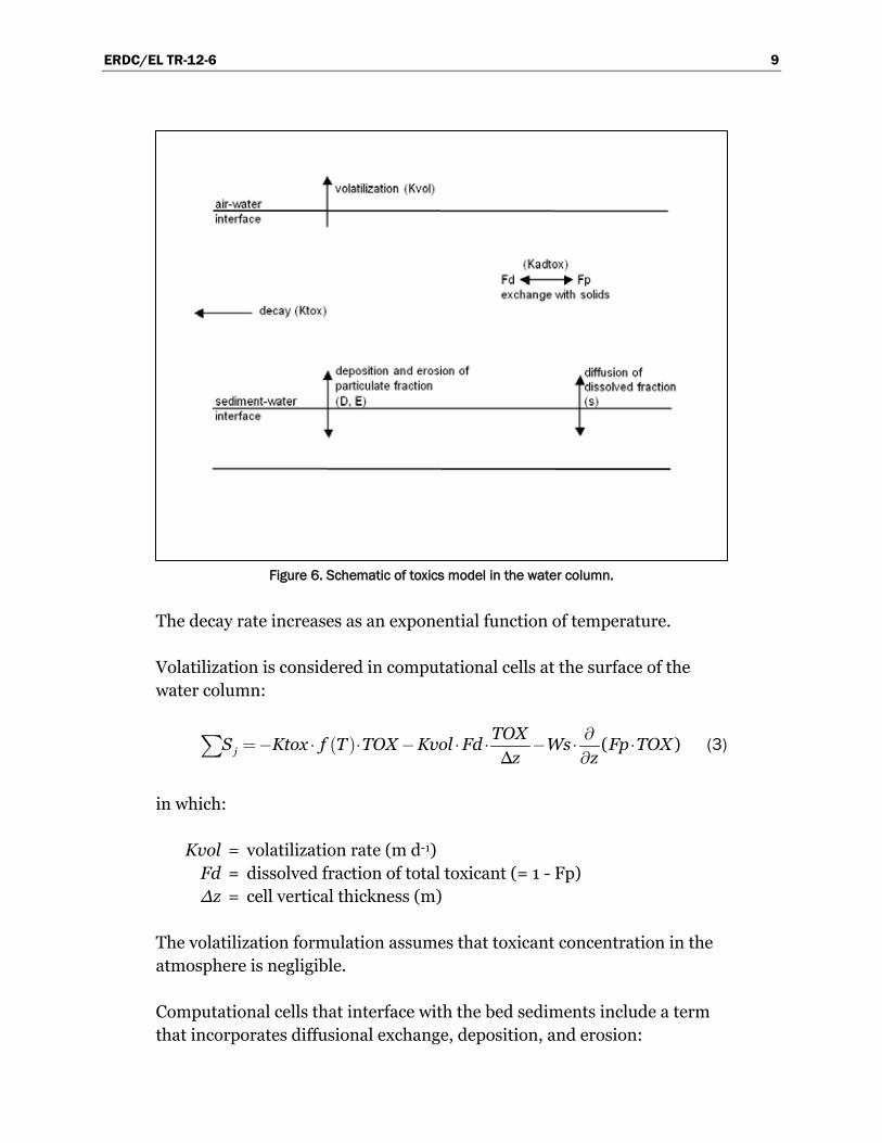
Internal sources and sinks (Figure 6) include the following:

• Exchange with the atmosphere (volatilization). • Decay. • Settling of particulate fraction. • Exchange with bed sediments (diffusion of dissolved fraction,

erosion/deposition of particulate fraction).

For a cell within the interior of the water column, the sources and sinks are represented as:

( ) jS Ktox f T TOX Ws Fp TOXz

(2)

in which:

TOX = toxicant concentration (g m-3) Ktox = decay rate at reference temperature T (d-1). Fp = particulate fraction of total toxicant (0 < Fp < 1) Ws = particle settling velocity (m d-1)

ERDC/EL TR-12-6 9

Figure 6. Schematic of toxics model in the water column.

The decay rate increases as an exponential function of temperature.

Volatilization is considered in computational cells at the surface of the water column:

( ) Δj

TOXS Ktox f T TOX Kvol Fd Ws Fp TOX

z z

(3)

in which:

Kvol = volatilization rate (m d-1) Fd = dissolved fraction of total toxicant (= 1 - Fp) Δz = cell vertical thickness (m)

The volatilization formulation assumes that toxicant concentration in the atmosphere is negligible.

Computational cells that interface with the bed sediments include a term that incorporates diffusional exchange, deposition, and erosion:

ERDC/EL TR-12-6 10

Δj

BENTOXS Ktox f T TOX Ws Fp TOX

z z

(4)

in which:

BENTOX = sum of exchange processes with the bed sediments (g m-2 d-1)

Settling into these cells from above is treated with the conventional ICM settling algorithms, but settling into the sediments is computed with SEDZLJ algorithms.

Particulate and dissolved fractions

For Toxicant 1, the particulate fraction is:

KADtox CSFp

KADtox CS

11 1

(5)

in which:

KADtox1 = toxicant 1 partition coefficient (m3 g-1) CS = clay/silt concentration (g m-3)

For Toxicant 2, the particulate fraction is:

( )( )

KADtox LPOC RPOCFp

KADtox LPOC RPOC

21 2

(6)

in which:

KADtox2 = toxicant 2 partition coefficient (m3 g-1 C) LPOC = labile particulate organic carbon (g C m-3) RPOC = refractory particulate organic carbon (g C m-3)

The dissolved fraction, for both toxicants, is:

Fd Fp 1 (7)

ERDC/EL TR-12-6 11

Toxics in the bed

The bed is envisioned as a single well-mixed layer with a thickness of ≈ 10 cm. The conceptualization is based on the observation that bioturba-tion forms a well-mixed sediment layer in a variety of locations and environ-ments (Boudreau 1998). The single well-mixed layer forms the basis for some of the earliest toxic models (O’Connor et al. 1983) and remains the basis for contemporary sediment diagenesis models (DiToro 2001). The RECOVERY model (Boyer et al. 1994) places a well-mixed layer at the sediment-water interface, above a succession of deeper layers.

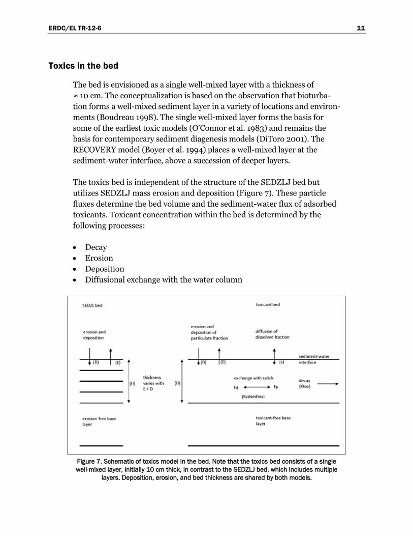
The toxics bed is independent of the structure of the SEDZLJ bed but utilizes SEDZLJ mass erosion and deposition (Figure 7). These particle fluxes determine the bed volume and the sediment-water flux of adsorbed toxicants. Toxicant concentration within the bed is determined by the following processes:

• Decay • Erosion • Deposition • Diffusional exchange with the water column

Figure 7. Schematic of toxics model in the bed. Note that the toxics bed consists of a single well-mixed layer, initially 10 cm thick, in contrast to the SEDZLJ bed, which includes multiple

layers. Deposition, erosion, and bed thickness are shared by both models.

ERDC/EL TR-12-6 12

The mass-balance equation for the bed is:

( )

δ H TOXsed

δtKtox H TOXsed D E s Fdw TOXw Fdsed TOXsed

(8)

in which:

H = thickness of toxics bed (m) TOXsed = toxicant concentration in bed (g m-3) TOXw = toxicant concentration in water (g m-3) Ktox = toxic decay rate in bed sediments (d-1) D = deposition rate of particulate toxicant (g m-2 d-1) E = erosion rate of particulate toxicant (g m-2 d-1) s = sediment-water mass-transfer velocity (m d-1) Fdw = dissolved fraction in water (0 < Fdw < 1) Fdsed = dissolved fraction in sediment (0 < Fds < 1)

The same mass-balance equation represents both toxicants; they sorb to different substances. Determination of dissolved and particulate fractions follows the formulation for the water column.

Deposition and erosion

SEDZLJ gives sediment deposition and erosion in terms of mass per unit area per model time-step. The deposition of toxicant 1 is then:

Δ

DclayD Fpw TOX w

t CS

1 1 (9)

in which:

Dclay = deposition of clay/silt (g m-2) CS = clay/silt concentration in water column (g m-3) Fpw = particulate fraction in water (0 < Fpw < 1) TOX1w = concentration of toxicant 1 in water column (g m-3) Δt = model integration time step (s)

The deposition of toxicant 2 is:

ERDC/EL TR-12-6 13

Δ

DpocD Fpw TOX w

t POC

1 2 (10)

in which:

Dpoc = deposition of labile and refractory particulate organic carbon (g m-2)

POC = labile plus refractory particulate organic carbon concentration in water column (g m-3)

TOX2w = concentration of toxicant 2 in water column (g m-3)

The erosion of toxicant 1 is:

Δ

EclayE Fpsed TOX sed

t BedCS

1 1 (11)

in which:

Eclay = erosion of clay/silt (g m-2) BedCS = clay/silt concentration in sediment bed (g m-3) TOX1sed = concentration of toxicant 1 in bed sediment (g m-3) Fpsed = particulate faction of toxicant in sediment

The erosion of toxicant 2 is:

Δ

EpocE Fpsed TOX sed

t BedPOC

1 2 (12)

in which:

Epoc = erosion of labile and refractory particulate organic carbon (g m-2)

BedPOC = labile plus refractory particulate organic carbon concentration in sediment bed (g m-3)

TOX2sed = concentration of toxicant 2 in bed sediment (g m-3)

Bed thickness

Toxicant concentration is defined as bulk concentration within the bed. The bulk concentration is influenced by changes in bed dimension as well as by

ERDC/EL TR-12-6 14

sources and sinks (Equation 8). The bed thickness at any instant is obtained by summing the sediment mass in each layer, divided by the bulk density:

( )( )

L Tsed LH

DryDens L

1

1

(13)

in which:

H = bed thickness (m) L = number of SEDZLJ sediment layers (The bottom layer is an

inert base for the active layers above) Tsed(L) = total sediment mass in layer L (g m-2) DryDens(L) = dry bulk density of sediment in layer L (g m-3)

ERDC/EL TR-12-6 15

4 Basic Performance Tests

A set of basic performance criteria was specified for acceptance of the merger of the SEDZLJ and ICM codes. The criteria were developed based on initial explorations of the linked models and included:

1. Mass conservation in water and bed. 2. Limited sensitivity to variations in model time-step. 3. Settling of new ICM state variables through model water column agrees

with settling of original ICM state variables. 4. Transport of new ICM state variables agrees with transport of original ICM

state variables. 5. Assurance that sediment bed will armor. 6. Evidence that bed erodes away smoothly. 7. Reasonable model behavior for accumulation in the bed with no erosion.

The same set of performance criteria is employed in exploration of the initial toxicant model coupled to SEDZLJ. The explorations are conducted on a 30-box grid (Figure 8) developed as an ICM test bed. Geometry and circulation in the test system are scaled to resemble the mainstem of Chesapeake Bay. The test bed provides the developer with maximum flexibility to examine model behavior via modifications to the ICM inputs and options installed in the ICM code.

Mass conservation

For this test, horizontal transport was eliminated. Mass conservation for a hydrophobic contaminant was examined in columns consisting of three water cells and five sediment layers. The toxicant bed was equated to the upper four sediment layers, each initially 5 cm thick. The bottom sediment layer formed an inert base for the active layers above. Active processes included vertical diffusion in the water column, settling, erosion, and deposition. Toxicant decay, volatilization, and diffusional exchange between the water column and bed were nullified to emphasize sedimentary processes. The time-step was 600 sec and test duration was five days. Two carbon forms, LPOC and RPOC, were considered. Initial conditions provided a uniform distribution of carbon and toxicant in the water column.

ERDC/EL TR-12-6 16

Figure 8. Elevation view of 30-box test grid. Cells are 30 km (length) x 20 km (width) x 5 m

(height).

Over the five-day period, carbon concentration in the water column increased due to erosion from the bed (Figure 9). A vertical concentration gradient appeared due to the interactions of settling, vertical diffusion, and erosion from the bed. A vertical gradient in toxicant concentration also developed, reflecting adsorption to the carbon forms (Figure 10). Roughly 0.009% of the initial carbon mass of each component was lost over the five-day period (720 time iterations, Table 1). Toxicant gained 0.435% although this statistic is adversely affected by the limited number of significant figures in the model print-out.

Figure 9. LPOC results from mass balance test. Initial and final concentrations are shown for three levels in the water column and for the sum of the upper four bed layers. Note that a vertical concentration gradient develops as material is eroded

from the bed. Results for RPOC are identical.

ERDC/EL TR-12-6 17

Figure 10. Toxicant results from mass balance test. Initial and final concentrations are shown for three levels in the water column and for the toxicant bed. Note that a vertical concentration gradient develops, which corresponds to the gradient in POC.

Table 1. Results from tests of mass conservation and sensitivity to time-step. Concentrations (g/m-2) are presented for a single column of water and sediment cells. Total final

concentrations should be identical to total initial concentrations.

Component Initial Concentration

Final Concentration, Δt = 60 sec

Final Concentration, Δt = 600 sec

Final Concentration, Δt = 2400 sec

LPOC, water 75 1,593.56 1,607.95 1,555.21

LPOC, sediments 33,000 31,487.40 31,464.20 31,517.13

LPOC, total 33,075 33,080.96 33,072.15 33,072.34

RPOC, water 75 1,593.56 1,607.95 1,555.21

RPOC, sediments 33,000 31,487.40 31,464.20 31,517.13

RPOC, total 33,075 33,080.96 33,072.15 33,072.34

Toxic, water 15 15.10 15.10 15.10

Toxic, sediments 2 1.98 1.97 1.98

Toxic, total 17 17.08 17.07 17.08

Model time-step

The mass conservation tests were repeated with two different time-steps: 60 sec and 2400 sec. The model demonstrated no degenerate behavior or

ERDC/EL TR-12-6 18

extreme sensitivity to the time-step (Table 1). Results were slightly different for each test, with mass potentially lost or gained. Results suggested a loss of accuracy in the carbon computation as the time-step was reduced to 60 sec. This result was unexpected. Usually, smaller time-steps yield greater accuracy due to reduced truncation error. For this experiment, however, it appeared that cumulative numerical round-off error, due to the larger number of iterations, outweighed the benefit from the order of magnitude reduction in time-step. The toxicant mass balance showed no distinct influence of time-step. As previously noted, toxicant mass balance appeared to be affected by the limited number of significant figures reported.

Settling velocity

ICM treats particle settling as a term in the kinetics formulations and codes. To ensure that settling of the toxicants agreed with results from previously tested and validated code, the adsorption coefficient of a hydrophobic contaminant, KADtox2, was set to 106 m3 g-1 C. Under this condition, the contaminant particulate fraction was effectively unity and the contaminant behavior should be identical to the carbon to which it was adsorbed. This test used the same conditions as the mass balance test except that erosion and deposition were eliminated. Settling velocity of POC was set to 1.32 m d-1 and the run was executed for 10 days. Particulate carbon and toxicant settled out of the surface and middle layers and accumulated in the bottom layer (Figures 11 and 12). Throughout the run, the relative changes in LPOC and toxicant were identical.

Transport

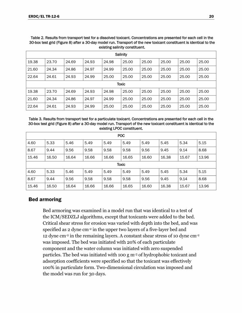
To ensure that transport of the toxicants agreed with previously tested and validated code, the parameter set was configured so toxicant 1 was completely dissolved and toxicant 2 was completely adsorbed to POC. Two-dimensional circulation similar to long-term average circulation in Chesapeake Bay was imposed. This run incorporated longitudinal and vertical currents, longitudinal and vertical diffusion, and vertical settling. Initial and boundary conditions for toxicant 1 were set identical to salinity. Initial and boundary conditions for toxicant 2 were set identical to LPOC. Under these circumstances, the transport of toxicant 1 should be the same as salinity while the transport of toxicant 2 should be the same as LPOC. At the end of a 10-day model run, these expectations were fulfilled. The concentrations of the new toxicant variables were identical to the concentrations of the existing model variables (Tables 2 and 3).

ERDC/EL TR-12-6 19

Figure 11. LPOC concentration during settling test. Concentration is normalized by initial

concentration and shown for three layers of a water column over a period of 10 days. Material settles out of the upper two layers and accumulates in the lower layer.

Figure 12. Toxicant concentration during settling test. Concentration is normalized by initial

concentration and shown for three layers of a water column over a period of 10 days. Settling of the new toxicant constituent is identical to the existing LPOC constituent.

ERDC/EL TR-12-6 20

Table 2. Results from transport test for a dissolved toxicant. Concentrations are presented for each cell in the 30-box test grid (Figure 8) after a 30-day model run. Transport of the new toxicant constituent is identical to the

existing salinity constituent.

Salinity

19.38 23.70 24.69 24.93 24.98 25.00 25.00 25.00 25.00 25.00

21.60 24.34 24.86 24.97 24.99 25.00 25.00 25.00 25.00 25.00

22.64 24.61 24.93 24.99 25.00 25.00 25.00 25.00 25.00 25.00

Toxic

19.38 23.70 24.69 24.93 24.98 25.00 25.00 25.00 25.00 25.00

21.60 24.34 24.86 24.97 24.99 25.00 25.00 25.00 25.00 25.00

22.64 24.61 24.93 24.99 25.00 25.00 25.00 25.00 25.00 25.00

Table 3. Results from transport test for a particulate toxicant. Concentrations are presented for each cell in the 30-box test grid (Figure 8) after a 30-day model run. Transport of the new toxicant constituent is identical to the

existing LPOC constituent.

POC

4.60 5.33 5.46 5.49 5.49 5.49 5.49 5.45 5.34 5.15

8.67 9.44 9.56 9.58 9.58 9.58 9.56 9.45 9.14 8.68

15.46 16.50 16.64 16.66 16.66 16.65 16.60 16.38 15.67 13.96

Toxic

4.60 5.33 5.46 5.49 5.49 5.49 5.49 5.45 5.34 5.15

8.67 9.44 9.56 9.58 9.58 9.58 9.56 9.45 9.14 8.68

15.46 16.50 16.64 16.66 16.66 16.65 16.60 16.38 15.67 13.96

Bed armoring

Bed armoring was examined in a model run that was identical to a test of the ICM/SEDZLJ algorithms, except that toxicants were added to the bed. Critical shear stress for erosion was varied with depth into the bed, and was specified as 2 dyne cm-2 in the upper two layers of a five-layer bed and 12 dyne cm-2 in the remaining layers. A constant shear stress of 10 dyne cm-2 was imposed. The bed was initiated with 20% of each particulate component and the water column was initiated with zero suspended particles. The bed was initiated with 100 g m-3 of hydrophobic toxicant and adsorption coefficients were specified so that the toxicant was effectively 100% in particulate form. Two-dimensional circulation was imposed and the model was run for 30 days.

ERDC/EL TR-12-6 21

The upper layer (5 cm) of the bed eroded into the water column immediately (Figure 13). Although gross erosion rate in the second layer was identical to the first layer, a portion of the previously eroded material simultaneously settled so that net erosion (erosion – deposition) slowed and the second layer took much longer than the first to disappear. Two unexpected results occurred as the upper two layers disappeared. The first was a decrease in the Layer 3 POC simultaneous with the complete erosion of Layer 2 (Figure 14). The second was the subsequent accumulation of material in Layer 3. Material settling into Layer 3, now at the bed surface, acquired the properties of Layer 3, notably critical shear stress. The thick-ness of this layer increased from 5 to nearly 7 cm as material accumulated; Layer 2 was not restored to replace the layer that previously disappeared.

Toxicant in the bed was examined in two systems of units, concentration per unit volume and concentration per unit area. On a volumetric basis, concentration diminished by a small amount at initiation of the run and then abruptly when POC was lost from Layer 3 (Figure 15). Volumetric concentration declined slowly thereafter as toxicant-free material settled into the bed and increased bed thickness but not bed toxicant. On an areal

Figure 13. Total bed mass during test of bed armoring. Layers 1 and 2 erode away while Layer

3 displays armoring. Note that material deposited after Layers 1 and 2 disappear acquires the characteristics (i.e. critical shear stress for erosion) of Layer 3.

ERDC/EL TR-12-6 22

Figure 14. LPOC concentration in three layers of the sediment bed during test of bed armoring. Note the apparent concentration change in Layer 3 simultaneous with the

disappearance of Layer 2.

Figure 15. Toxicant concentration during test of bed armoring. Concentration, on a volumetric basis, shows sharp decreases at the initiation of erosion and simultaneous with the apparent

loss of POC from Layer 3. Concentration, on an areal basis, remains constant after the bed armors.

ERDC/EL TR-12-6 23

basis, toxicant was lost abruptly at initiation of the run and then slowly while Layer 2 eroded away. Subsequently, the areal concentration remained constant since the coarse material settling into Layer 3 carried no toxicant.

This test indicated that the physical process of bed armoring proceeded satisfactorily. The factors contributing to the apparent loss of POC from Layer 3 simultaneous with the disappearance of Layer 2 require further investigation.

Continuous erosion

For this test, critical shear stress for erosion was varied with depth into the bed. Critical shear stress varied from 2 dyne cm-2 in the upper three layers to 5 dyne cm-2 in Layer 4, to 20 dyne cm-2 in Layer 5. Continuous shear stress of 19 dyne cm-2 was imposed. The test was designed to erode away the upper four layers, which comprised the toxic bed, while leaving the toxicant-free base layer. Erosion proceeded as envisioned. The upper four layers eroded successively into the water column (Figure 16). No erosion of the bottom layer occurred although previously eroded sand accumulated in this layer, increasing the initial mass. This phenomenon duplicated the accumulation of previously eroded material noted during the test of bed armoring. Toxicant disappeared from the bed simultaneous with the complete erosion of the upper four layers (Figure 17). The remaining base layer remained toxicant-free despite the accumulation of sand, since no toxicant was sorbed to the sand constituents.

Continuous deposition

Two tests of continuous deposition were conducted. The first examined the continuous deposition of clean sediment onto a toxic bed. The second examined the continuous deposition of sediment containing a sorbed toxicant onto a toxic bed. For these tests, shear stresses were specified so that erosion would not occur. Initial conditions and boundary conditions in the water column were specified to provide a large reservoir of material capable of settling. Two-dimensional circulation was enabled and the model was run for 30 days.

Material accumulated continuously in the surface sediment layer in both tests (Figure 18). By the end of the runs, Layer 1 bed mass more than doubled. In the first test, which involved the deposition of clean sediment,

ERDC/EL TR-12-6 24

Figure 16. Bed mass during test of continuous erosion. The upper four bed layers erode

immediately. The bottom layer resists erosion but acquires material through settling.

Figure 17. Toxicant concentration during test of continuous erosion. Toxicant disappears from

the bed simultaneous with the depletion of the upper four sediment layers.

ERDC/EL TR-12-6 25

Figure 18. Bed mass during test of continuous deposition. Material accumulates in the

surface layer throughout the test.

the amount of toxicant in the bed remained constant, on an areal basis (Figure 19). Concentration, however, diminished as the volume of the bed increased. This run reinforced the findings from the tests of bed armoring; the thickness of the surface layer increased as material accumulated but no new layer was created despite the large amount of material deposited. The implication of this behavior is significant. The deposition of clean sediment did not bury toxicants. Rather, toxicant was dispersed throughout the newly deposited material and remained at the sediment-water interface at all times.

The second test proceeded as expected. Toxicant in the bed accumulated continuously as material bearing sorbed toxicant was deposited (Figure 20). Toxicant concentration increased by orders of magnitude with no aberrant effects.

ERDC/EL TR-12-6 26

Figure 19. Toxicant concentration during test of continuous deposition. Deposition of clean

material dilutes the concentration of toxicant. On an areal basis, the amount of toxicant in the bed remains constant. Note that toxicant is not buried by the accumulation of clean material.

Figure 20. Toxicant concentration during test of continuous deposition. Deposition of sorbed

toxicant adds to the bed throughout the run.

ERDC/EL TR-12-6 27

5 Summary and Conclusions

The preceding chapters described two tasks. The first was the conversion of the combined ICM/SEDZLJ computer codes to parallel operation. The conversion resulted in order-of-magnitude speed-up of the combined codes with no adverse effects on the computation. Results from parallel operation were identical to serial operation for up to 128 processors.

The second task was the incorporation of an initial toxics code into the combined ICM/SEDZLJ codes. Two toxicants were considered. The first partitioned to clay/silt particles in the water and bed sediments. The second partitioned to particulate organic carbon. The treatment of the new variables in the water column was analogous to the three-dimensional, finite-volume approach used for the other ICM state variables. In the bed, toxics were considered to occupy a single well-mixed layer roughly 10 cm in thickness. This approach was adopted from the ICM sediment diagenesis model. Particle deposition and erosion and the resulting effects on bed thickness were taken from SEDZLJ. This framework formed the basis for a unified model of the aquatic carbon cycle, of particulate transport, and of toxicant processes.

The new code was subjected to a series of tests patterned after tests developed to examine the behavior of the combined ICM/SEDZLJ models. The performance criteria included:

1. Mass conservation in water and bed. 2. Limited sensitivity to variations in model time-step. 3. Settling of new ICM state variables through model water column agrees

with settling of original ICM state variables. 4. Transport of new ICM state variables agrees with transport of original ICM

state variables. 5. Assurance that sediment bed will armor. 6. Evidence that bed erodes away smoothly. 7. Reasonable model behavior for accumulation in the bed with no erosion.

The tests can be divided into two classes: criteria that the model must fulfill; and examinations of model behavior. Criteria that must be fulfilled include mass conservation and consistency of settling and transport with

ERDC/EL TR-12-6 28

previous model results. The new code performed satisfactorily for these criteria. Additional attention towards the accuracy of mass conservation is warranted during further model developments, however. The model formulations appear correct but numerical precision during the extensive computations in the sediment bed may be affecting results.

The remaining tests were examinations of model behavior as a result of various forcing functions. The model showed no undue sensitivity to the time-step and continued to perform under extreme conditions such as complete erosion of the toxicant bed.

An artifact noted during the testing of the ICM/SEDZLJ codes carried through to these tests as well. When a bed layer is completely eroded, it is gone permanently. Material that subsequently settles is added to the upper-most existing bed layer. The eroded layer does not reappear. Physically, the newly deposited material acquires the characteristics of the existing bed layer. The implication for the existing toxics model, and for more detailed models built on the SEDLZJ framework, is that deposition of clean material will not bury toxicant. Rather, toxicant will mix with the newly deposited material and remain at the sediment-water interface.

Use of a well-mixed sediment bed of constant thickness is a common approach to sediment bed chemistry. Coupling of the well-mixed bed with dynamic particle fluxes at the sediment-water interface reveals some weaknesses, however, in the combination. The first is that the thickness of the bed is no longer constant. The tests run here were extreme in the change of bed thickness compared to the changes likely to be encountered in a stable prototype system. Still, the potential for extreme bed changes during extreme events must be considered. A second problem, which has not been completely characterized, is the loss of POC from an armored layer simultaneous with the complete erosion of the layer above.

The toxicant model described in this note provides an initial, successful step in the development of a unified model of the aquatic carbon cycle, of particulate transport, and of toxicant processes. The next step is to develop a detailed, multi-layered toxicant bed model consistent with the physical bed described by SEDZLJ.

ERDC/EL TR-12-6 29

References Boudreau, B. 1998. Mean mixed depth of sediments: The wherefore and the why.

Limnology and Oceanography 43(3):524-526.

Boyer, J., S. Chapra, C. Ruiz, and M. Dortch. 1994. RECOVERY, A mathematical model to predict temporal response of surface water to contaminated sediments. Technical Report W-94-4. Vicksburg, MS: U.S. Army Engineer Waterways Experiment Station.

Cerco, C., and T. Cole. 1994. Three-dimensional eutrophication model of Chesapeake Bay. Technical Report EL-94-4. Vicksburg MS: U.S. Army Engineer Waterways Experiment Station.

Cerco, C., M. Noel, and S-C. Kim. 2004. Three dimensional dutrophication model of Lake Washington, Washington State. Technical Report ERDC/EL TR-04-12. Vicksburg, MS: U.S. Army Engineer Research and Development Center.

Cerco, C. Combining the ICM eutrophication model with the SEDZLJ sediment transport model. In preparation. Vicksburg, MS: U.S. Army Engineer Research and Development Center.

Chippada, S., C. Dawson, V. Parr, M. Wheeler, C. Cerco, B. Bunch, and M. Noel. 1998. PCE-QUAL-ICM: A parallel water quality model based on CE-QUAL-ICM. CRPC-TR-98766. Houston TX: Center for Research on Parallel Computation, Rice University. (Available on line as http://softlib.rice.edu/pub/CRPC-TRs/reports/CRPC-TR98766.pdf)

DiToro, D. 2001. Sediment flux modeling. New York: John Wiley and Sons, 27-55.

Jones, C., and W. Lick. 2001. SEDZLJ, a sediment transport model. Santa Barbara, CA: Department of Mechanical and Environmental Engineering, University of California.

Noel, M., T. Gerald, and C. Cerco. 2000. Parallel performance and benchmarking of the CE-QUAL-ICM family of three-dimensional water quality models. In Applications of high performance computing VI: International conference on applications of high-performance computing in engineering. Maui, HI. Southamptom GB: WIT press, 301-309.

O’Connor, D., J. Mueller, and K. Farley. 1983. Distribution of kepone in the James River Estuary. Journal of Environmental Engineering 109(2):396-413.

Tetra Tech Inc. 2007. The Environmental fluid dynamics code, theory and computation, Volume 2: Sediment and contaminant transport and fate. Fairfax, VA: Tetra Tech Inc.

U.S. Environmental Protection Agency (USEPA). 1987. User’s manual for the chemical transport and fate model TOXIWASP Version 1. EPA-600/3-837005. Athens, GA.

REPORT DOCUMENTATION PAGE Form Approved

OMB No. 0704-0188 Public reporting burden for this collection of information is estimated to average 1 hour per response, including the time for reviewing instructions, searching existing data sources, gathering and maintaining the data needed, and completing and reviewing this collection of information. Send comments regarding this burden estimate or any other aspect of this collection of information, including suggestions for reducing this burden to Department of Defense, Washington Headquarters Services, Directorate for Information Operations and Reports (0704-0188), 1215 Jefferson Davis Highway, Suite 1204, Arlington, VA 22202-4302. Respondents should be aware that notwithstanding any other provision of law, no person shall be subject to any penalty for failing to comply with a collection of information if it does not display a currently valid OMB control number. PLEASE DO NOT RETURN YOUR FORM TO THE ABOVE ADDRESS.

1. REPORT DATE (DD-MM-YYYY) March 2012

2. REPORT TYPE Final report

3. DATES COVERED (From - To)

4. TITLE AND SUBTITLE

Incorporation of Chemical Contaminants into the Combined ICM/SEDZLJ Models

5a. CONTRACT NUMBER

5b. GRANT NUMBER

5c. PROGRAM ELEMENT NUMBER

6. AUTHOR(S)

Carl F. Cerco

5d. PROJECT NUMBER

5e. TASK NUMBER

5f. WORK UNIT NUMBER

7. PERFORMING ORGANIZATION NAME(S) AND ADDRESS(ES) 8. PERFORMING ORGANIZATION REPORT NUMBER

U.S. Army Engineer Research and Development Center Environmental Laboratory 3909 Halls Ferry Road Vicksburg, MS 39180

ERDC/EL TR-12-6

9. SPONSORING / MONITORING AGENCY NAME(S) AND ADDRESS(ES) 10. SPONSOR/MONITOR’S ACRONYM(S)

11. SPONSOR/MONITOR’S REPORT NUMBER(S)

12. DISTRIBUTION / AVAILABILITY STATEMENT

Approved for public release; distribution is unlimited.

13. SUPPLEMENTARY NOTES

14. ABSTRACT

This report describes two tasks. The first is the conversion of the combined ICM/SEDZLJ computer codes to parallel operation. The conversion results in order-of-magnitude speed-up of the combined codes with no adverse effects on the computation. Results from parallel operation are identical to serial operation for up to 128 processors.

The second task is the incorporation of an initial toxics code into the combined ICM/SEDZLJ codes. Two toxicants are considered. The first partitions to clay/silt particles in the water and bed sediments. The second partitions to particulate organic carbon. Treatment of the new variables in the water column is analogous to the three-dimensional, finite-volume approach used for the other ICM state variables. In the bed, toxics are considered to occupy a single well-mixed layer roughly 10 cm in thickness. This approach is adopted from the ICM sediment diagenesis model. Particle deposition and erosion and the resulting effects on bed thickness are taken from SEDZLJ. This framework forms the initial basis for a unified model of the aquatic carbon cycle, of particulate transport, and of toxicant processes.

15. SUBJECT TERMS

CE-QUAL-ICM model Contaminant fate and transport model

Contaminants ICM model SEDZLJ model

16. SECURITY CLASSIFICATION OF: 17. LIMITATION OF ABSTRACT

18. NUMBER OF PAGES

19a. NAME OF RESPONSIBLE PERSON

a. REPORT

UNCLASSIFIED

b. ABSTRACT

UNCLASSIFIED

c. THIS PAGE

UNCLASSIFIED 36 19b. TELEPHONE NUMBER (include area code)

Standard Form 298 (Rev. 8-98) Prescribed by ANSI Std. 239.18