ergodic theory and dynamical systems 25, 2005, pp. 661-709afisher/ps/anoffamfinal010604a.pdf ·...
TRANSCRIPT

Ergodic Theory and Dynamical Systems 25, 2005, pp. 661-709(this preprint version contains all final changes)
ANOSOV FAMILIES, RENORMALIZATION AND NONSTATIONARYSUBSHIFTS
PIERRE ARNOUX AND ALBERT M. FISHER
Abstract. We introduce the notion of an Anosov family, a generalization of an Anosov map of amanifold. This is a sequence of diffeomorphisms along compact Riemannian manifolds such that thetangent bundles split into expanding and contracting subspaces.
We develop the general theory, studying sequences of maps up to a notion of isomorphism andwith respect to an equivalence relation generated by two natural operations, gathering and dispersal.
Then we concentrate on linear Anosov families on the two-torus. We study in detail a basic classof examples, the multiplicative families, and a canonical dispersal of these, the additive families.These form a natural completion to the collection of all linear Anosov maps.
A renormalization procedure constructs a sequence of Markov partitions consisting of two rect-angles for a given additive family. This codes the family by the nonstationary subshift of finite typedetermined by exactly the same sequence of matrices.
Any linear positive Anosov family on the torus has a dispersal which is an additive family. Theadditive coding then yields a combinatorial model for the linear family, by telescoping the additiveBratteli diagram. The resulting combinatorial space is then determined by the same sequence ofnonnegative matrices, as a nonstationary edge shift. This generalizes and provides a new proof fortheorems of Adler and Manning.
Contents
1. Introduction 11.1. Motivation: a completion for Anosov maps 11.2. Structure of the paper 31.3. Anosov families 31.4. Anosov families as mapping families: morphisms, gatherings and dispersals 41.5. Coding the additive and multiplicative families: nonstationary subshifts 51.6. Further generalizations 61.7. Acknowledgements 72. Mapping families. 72.1. Sequences of maps; conjugacy and equivalence 72.2. Hyperbolicity 113. Symbolic dynamics of mapping families. 193.1. Partition sequences 193.2. Markov partitions 203.3. Nonstationary subshifts 223.4. Symbolic dynamics for Anosov families 25
Date: October 31, 2003.Key words and phrases. Anosov family, renormalization, continued fraction, Markov partition, nonstationary
subshift, Bratteli diagram, random dynamical sytstem .1

2 PIERRE ARNOUX AND ALBERT M. FISHER
3.5. Nonstationary vertex and edge shift spaces and and Bratteli diagrams 263.6. The (2× 2) case: additive sequences and canonical labelings 294. The multiplicative family. 314.1. Box renormalization and the construction of Markov Partitions. 354.2. Producing a generator: the Adler-Weiss method 375. An extension of theorems of Adler and Manning to mapping families 385.1. Additive and linear families 395.2. A Markov Partition and symbolic dynamics for the additive family 405.3. Gathering, connected components, and symbolic dynamics 415.4. Application: An Adler-Manning type coding for a random dynamical system 43References 44
1. Introduction
When studying dynamics, one usually considers the iterates of a single transformation on a fixedspace. Here we are interested in the dynamical behavior of a sequence of maps, along a sequence ofspaces. Although at first glance the dynamics of a sequence of maps is trivial (since it is wandering),for the examples we will study here, one can find all of the richness of a recurrent dynamical system.
1.1. Motivation: a completion for Anosov maps. Sequences of maps arise naturally in avariety of ways; see Examples 1-6 in §1. The objects studied in this paper can be looked at from acorresponding variety of viewpoints.
We choose one of these as our primary motivating idea. We consider the set of all orientation-preserving linear Anosov diffeomorphisms on the two-torus, and ask this question: what would bea natural notion of completion for this collection of dynamical systems? For a first attempt at ananswer, let us associate to a map A its pair of expanding and contracting foliations. These arenumerically special, as the slopes of the foliations belong to the (dense) set of quadratic irrationals.Looking only at the foliations, it is natural to take as a completion, then, the collection of all pairsof transverse linear foliations.
For a notion of completion to be reasonable, the important dynamical structures associated withthe individual maps should pass over to the new points, by continuity.
In fact, certain structures do extend naturally to this provisional completion: the unstable flowsand their return (holonomy) maps, which in this case is the completion from circle rotations ofquadratic type to all rotations.
Moreover, the usual Berg-Adler-Weiss construction of Markov partitions [AW70], [Adl98], (or atleast its first step, the construction of a pair of parallelograms from eigenline segments) depends inno way on the special character of the Anosov slopes and so extends to this completion.
But what is iteration, where is the hyperbolic dynamics, when one begins just with a pair offoliations? Indeed, we say “first step” of the construction here because the second step is moreproblematic: making a generator (a partition which separates points under iteration) from this pairof boxes. Here we recall the process Adler and Weiss used in building a generator: one pulls backthe two-box partition from the future via the map, and then takes connected components of theresulting intersections with the present partition. See Fig. 12.

ANOSOV FAMILIES, RENORMALIZATION AND NONSTATIONARY SUBSHIFTS 3
Apparently this uses in an essential way the dynamics. But in fact, if we consider closely thegeometry of the resulting partition, we can find a way to build this partition without any referenceto the hyperbolic dynamics.
The key observation is that the new partition also can be specified directly from the pair of circlerotations, in terms of their joint renormalization; one is renormalized and the other un-renormalized.So at least some sense can be made of generation in this setting. And in this way, even withoutdynamics, one can define the “itinerary” of a point, associating to it a symbol sequence.
However the mystery remains: where is the dynamics? And how can that be seen as an extensionof the dynamics of the individual maps to this completion?
What we do is change the initial set-up, and instead of representing each Anosov map A by itspair of foliations, we represent it by a biinfinite sequence of maps, repeating periodically, givenby a factorization of A. To do this in a canonical way we use a (well-known) representation oforientation-preserving nonnegative (2×2) integer matrices as a product of two positive Dehn twists,see Lemma 3.11. Then, our completion will be all sequences of maps, given by those generators;and the dynamics takes us along a sequence of distinct copies of the torus.
It then turns out that the two-box Markov partition sequence is itself a generator for this se-quence of maps, and moreover that the previous construction (pulling back and taking connectedcomponents) can be understood directly from that fact. See Lemma 5.4.
Having defined our candidate for the completion, a first question is whether the basic definingproperty of the Anosov maps (the hyperbolic splitting with contraction bounds) extends to thiscompletion. The answer is yes, if we first remove a countable dense set. These correspond to therational angles, which are also exactly those angles for which the renormalization of the rotationsbreaks down after a finite number of steps.
1.2. Structure of the paper. There are three main circles of results in this paper. The first,given in §2, involves general results on mapping and Anosov families. This provides an appropriatecontext and language for the rest of the paper.
In the second part, in §3, we introduce the symbolic dynamics for families, given by sequences ofpartitions. For the case of Anosov families, this specializes to Markov partition sequences and thecorresponding symbolic spaces, given by a nonstationary sequence of 0−1 matrices and geometricallyrepresented by two-sided Bratteli diagrams.
In the third circle of results, presented in §§4 and 5 , we focus on a class of specific examples onthe two-torus, which illustrate and give form to these abstract ideas.
These examples, the multiplicative and additive families, are related to the idea of a completionof the Anosov toral maps discussed above.
In the rest of the Introduction we summarize the main results.
1.3. Anosov families. To understand the new elements of the above completion, and what is thenature of dynamics for them, we introduce this notion:
Definition. An Anosov family is a (biinfinite) sequence of diffeomorphisms along a sequence ofcompact Riemannian manifolds, with an invariant sequence of splittings of the tangent bundle intoexpanding and contracting subspaces, and with a uniform upper bound for the contraction andlower bound for the expansion.
Similarly, an eventually Anosov family has the invariant splitting but now the contraction andexpansion only are required to happen after an (unbounded) number of iterates.

4 PIERRE ARNOUX AND ALBERT M. FISHER
Proposition. An (eventually) Anosov splitting is unique if it exists.
(See Proposition 2.2.)It is important to know this, since with wandering dynamics, any splitting can be made invariant
simply by transporting it along the sequence of spaces.Here are our main examples.
Definition. Given a sequence (ni) = (. . . , n−1, n0, n1 . . . ) for ni ∈ N∗ = 1, 2, . . . , we define
matrices Ai ∈ SL(2,Z) by: Ai =
[1 0ni 1
]for i even, Ai =
[1 ni0 1
]for i odd. We let the Ai act
on the torus; each choice of (ni) defines a sequence of maps along a sequence of tori, which we shallcall a multiplicative family because of its relation to the multiplicative continued fraction.
Our second basic example, the additive family, is given by factoring a multiplicative family; thus
we take all biinfinite sequences of matrices of the form
[1 01 1
]and
[1 10 1
], the additive generators,
which is nontrivial in the sense that the type of the matrix changes infinitely often at ±∞.
We show:
Theorem. Each multiplicative family is an Anosov family; indeed the slopes of the contracting andexpanding directions on the component Mi are related in a simple way to the continued fractions
[nini+1 . . . ] =1
ni +1
ni+1 + · · ·and [ni−1ni−2 . . . ] respectively (for the precise statement see Proposition 4.1.)
We have as a consequence:
Theorem. Any nontrivial additive family is an eventually Anosov family; its eigendirections aregiven by the corresponding additve continued fractions.
Our completion, the collection of multiplicative families, is parametrized by the product Π∞−∞N∗,with the Anosov maps themselves corresponding exactly to periodic sequences (ni).
1.4. Anosov families as mapping families: morphisms, gatherings and dispersals. Thesequences of maps discussed above are part of a larger abstract context, which provides a clearerperspective on the Anosov and eventually Anosov families.
To describe this general setting, we consider sequences of maps as a category with respect tocertain types of homomorphism, and also introduce a notion of equivalence generated by two naturaloperations: gathering and dispersal.
Definition. A mapping family is a sequence of continuous maps along a sequence of compact metricspaces, called components. A uniform conjugacy from one mapping family to another is given byan equicontinuous sequence of conjugating maps.
Remark. This notion of morphism makes the collection of all mapping families into a category. Thereason for not considering the topological category- and using topological instead of metric spaces,and topological instead of uniform conjugacy- is that for mapping families there is no topologicaldynamics: every family is topologically conjugate to the trival family whose maps are all the identity,see Proposition 2.1.

ANOSOV FAMILIES, RENORMALIZATION AND NONSTATIONARY SUBSHIFTS 5
For the uniform category, on the other hand, despite the fact that a mapping family has norecurrence (each component is a wandering set) the basic dynamical structures of stable and unstablesets make sense, as we have by Proposition 2.2 and Corollary 2.3:
Theorem. Stable and unstable sets are preserved by uniform conjugacies hence are well-definednotions in the category of mapping families.
Definition. For the category of smooth mapping families (C1 mapping families along a sequence ofcompact manifolds with Riemannian metrics) we define the morphisms to be bounded conjugacies(to have uniform bounds on the derivatives).
Thus bounded conjugacies preserve expansion bounds up to a constant. Hence we have (Propo-sition 2.14):
Theorem. The Anosov and eventually Anosov families are categories with respect to bounded con-jugacy.
Definition. A gathering of a mapping family is a family given by taking of partial compositionsalong a subsequence; a dispersal is its converse, a factorization.
A basic example of dispersal is given by the insertion of extra copies of the identity map. Fora second example, note that an additive family gathers to the corresponding multiplicative familyand that conversely the additive family is a dispersal of the multiplicative family.
Remark. These are natural operations to consider for general mapping families but one must becareful: by contrast with uniform conjugacy, the operations of gathering and dispersal do notpreserve the dynamical structures of stable and unstable sets; see Proposition 2.5.
However, as we show in Corollary 2.13, see also Remark 2.13:
Theorem. Within the category of eventually Anosov families, stable and unstable sets are preservedby the operations of gathering and dispersal.
1.5. Coding the additive and multiplicative families: nonstationary subshifts. A key toolfor the further study of additive and multiplicative families is the extension of the notion of Markovpartition to sequences of maps. The associated symbolic representation will be a combinatoriallydefined mapping family which we call a nonstationary subshift of finite type (nsft).
We begin in the setting of mapping families. One still has (as for single maps) a notion of codingthe dynamics by the itineraries of a point, but now instead of this being described by where theorbit is located with respect to a single partition, this “name” of the point will now be given by asequence of partitions along the sequence of spaces.
We generalize Markov partitions in the natural way; the new phenomenon is that in this setting,the symbolic space is now defined by a sequence of rectangular transition matrices (i.e. with entries0 and 1), replacing the single square matrix which defines a subshift of finite type (sft).
The resulting space is a two-sided version of what Vershik and Livshits [VL92] call a Markovcompactum.
As such, this space has no shift defined on it as the transitions keep changing. We introduce shiftdynamics by taking the disjoint union of all compacta defined by shifts of the transition matrixsequence. This space is now a mapping family, whose components are simply all the shifts of theoriginal Markov compactum.

6 PIERRE ARNOUX AND ALBERT M. FISHER
Definition. This total space (the compactum together with all its shifts), is a nonstationary subshiftof finite type (nsft).
This gives a second, combinatorial mapping family, which as is the case for a single map, factorsonto the original family, provided the partition sequence generates (Proposition 3.6).
For our main examples, the additive and multiplicative families, we construct explicit Markovpartitions. To do this, first we define a sequence of pairs of parallelograms (boxes) given by a simplealgorithmic procedure related to continued fractions. For the additive family things are simplest.We show (Lemma 5.2):
Theorem. Given a nontrivial additive family, the box pairs give a generating Markov partitionsequence.
For the multiplicative families, the two-box partition is Markov but does not generate. The sameidea used by Adler and Weiss for a single map works here:
Theorem. Given a multiplicative family, the partition sequence given by taking connected compo-nents of the join of each two-box partition with the pullback of the succeeding one gives a Markovpartition sequence which generates.
See Proposition 4.6. Now we apply the abstract machinery developed before (gatherings ofmapping families) to see this construction in a new way, see Lemma 5.4:
Theorem. The (generating) connected component partitions of a multiplicative family are alterna-tively given by gathering the two-box partition sequence of the corresponding additive family.
Next we describe the nonstationary subshifts of finite type defined by these Markov partitionsequences. First we have, for a nontrivial additive family (Theorem 5.3):
Theorem. The mapping family is symbolically represented by the nsft given by exactly the samesequence of 0− 1 matrices, now interpreted as transition matrices.
See Lemma 5.4.The symbolic version of gathering corresponds to what is known in the theory of Bratteli diagrams
as the telescoping of the diagram. The general theory, developed in §§3.1- 3.5, allows us to extendthe previous result to multiplicative families, and further to the mapping family defined by a generalsequence of (2 × 2) matrices in SL(2,N), the semigroup of matrices with determinant 1 and withnonnegative integer entries.
The conclusion is (Theorems 5.1 and 5.6):
Theorem. Given a mapping family defined by a nontrivial sequence of matrices in SL(2,N) actingon the two-torus, then:(i) this is an Anosov family, and(ii) it has a generating Markov partition sequence which codes it as the nsft defined as an edge shiftby exactly the same sequence of matrices.
Restricting to the case of a single map gives a new proof of a theorem of Adler on codings ofAnosov maps: that an orientation-preserving (2× 2) Anosov matrix with nonnegative entries has aMarkov partition for which it itself gives the edge shift space. See Theorem 5.3. Anthony Manning[Man02] proved a result similar to Adler’s, but got the transpose matrix instead.

ANOSOV FAMILIES, RENORMALIZATION AND NONSTATIONARY SUBSHIFTS 7
Remark. To get a statement like Adler’s one needs to consistently choose the same convention formatrix actions, using either the action on rows or on columns both for the toral action and fordefining the combinatorial spaces. Throughout this paper we use the column-vector convention.Mixing the conventions gives the transpose, as in Manning’s version of the theorem. The reason forthis becomes especially transparent when seen from the mapping family point of view; see Remark5.3.
1.6. Further generalizations. There are several natural directions for extending this work andthat of [AF01] and [AF02a]: to the orientation-reversing case, to higher genus surfaces, to higherdimensional tori, and to nonlinear Anosov maps. We plan to develop this material in a seriesof papers. In particular, we have linear, topological and smooth classification theorems of Anosovfamilies on the two-torus, and a topological classification on the n-torus. As a corollary we can solvea question asked by Kifer (Conjecture A1 of [Kif00]). We mentioned above that there is no shiftdynamics on a single component of an nsft; however one can define there a transversal dynamics,given by Vershik’s adic transformations; see [Ver94]. Equivalently the tranversal dynamics can bedefined by nonstationary substitution systems. We do not discuss these fascinating topics in thepresent paper; see [AF02b], [AF02a], [AF01]. In work of A. F. with M. Urbanski, we prove theexistence of a Markov partitions for an Anosov family, generalizing the construction of [Bow75],[Bow77]. The main case studied in the present paper is simpler so we can we construct the partitionsexplicitly, see §4.
Another natural generalization is from discrete to continuous time: from mapping families towhat could be called flow families. One example is the suspension flow of a mapping family. Thesuspension of a multiplicative family is an interesting object for an entirely different reason: itmodels the scenery flow of the transverse irrational circle rotation. See [AF02a], [AF01]. A furtherpotentially interesting class of examples to consider are the flow families given by nonautonomousdifferential equations, where the orbits are integral curves of time-varying vector fields.
1.7. Acknowledgements. This work draws from many different parts of dynamical systems the-ory, and so builds on research of many people, too numerous to mention here. The project originallycame out of an attempt to put together the ideas of [Fis92] on the scenery flow for a fractal set and[Arn94] on the Teichmuller flow, and in particular owes much to the work of Veech. The connectionsof these flows with the present work is made in [AF02a]; see also [Fis04], [Fis03].
The name “families” we borrowed from David Rand’s Markov families of expanding maps onthe interval [Ran88], see Remark 2.17 below. We mention that V.I. Bakhtin also has considerednon-random hyperbolic sequences of mappings [Bak95a], [Bak95b], studying nonlinear theory; wethank Y. Kifer for this citation.
The second-named author would like to thank the following institutions and agencies for theirsupport and hospitality during the course of the writing: IHES; the Graduate Center at CUNY;the CNRS and Univ. Paris XIII; the IMS and SUNY Stony Brook; the CNPQ and FAPERGS atUFRGS Porto Alegre, Brazil; IMPA; the CNPQ at the University of Sao Paulo; the CNRS and theUniversity of Marseilles, Luminy.
We would like to thank all the many colleagues who have inspired and aided us along the way.Special thanks for related conversations and for their interest, inspiration and encouragement goesto: Elise Cawley, Matthias Gundlach, Pascal Hubert, Jeremy Kahn, Rick Kenyon, Curt McMullen,Yair Minsky, Alberto Pinto, Tom Schmidt, and Dennis Sullivan.
8 PIERRE ARNOUX AND ALBERT M. FISHER
2. Mapping families.
2.1. Sequences of maps; conjugacy and equivalence. We begin with a discussion of sequencesof maps in several categories, considering topological, uniform and bounded differentiable conju-gacies as providing the morphisms. Then we introduce two operations, gathering and dispersal.Lastly we study the interplay between change of metric and dynamics, for which purpose we con-sider isometric conjugacy.
A key conclusion will be that for families, the spaces should have a uniform structure, with themorphisms preserving that uniformity. For simplicity, we work in the category of metric spaceswith uniformly continuous maps. We show that furthermore, gathering and dispersal are not wellbehaved operations in complete generality, but do make sense in the presence of hyperbolicity.Finally, we see that any dynamics can be pushed entirely to the metrics, and that a converse isalso true, provided the minimum necessary requirement of having isometric spaces is satisfied. Thisabstract framework will be illustrated in the next section by concrete examples.
Given a sequence of sets Mi for i ∈ Z, the disjoint union written M =∐Mi is the coproduct
in the category of sets, see e.g. [Hun74]. We recall that this is simply the indexed union; that is, apoint in M is a point p in some Mi together with the index i. For convenience we will suppress thisindex and write p for this point; thus, any p ∈ M belongs to exactly one Mi. We refer to the Mi
as components of M . If the components are topological spaces, then we topologize M by puttingthese spaces together discretely. By this we mean the topology is generated by the union of allthose topologies, so in particular each Mi itself is open and closed in M . (Warning: a componentMi may itself have more than one topological component; an example is given by the nonstationaryshift space of §3.1).
Definition 2.1. Let Mi for i ∈ Z be a sequence of metric spaces with metrics ρi. Assume forsimplicity that the diameter of each space is less than or equal to 2. We give the total space themetric ρ(x,w) = ρi(x,w) if x,w ∈ Mi, = 1 if they are in different components (the bound of 2ensures that one has the triangle equality). We assume fi : Mi → Mi+1 are continuous functions.We define the total map f : M → M on the disjoint union to be equal to fi on each componentMi. The nth composition fn maps Mi to Mi+n and is equal to fi+n · · · fi on Mi for each i. Wewill call the resulting pair (M, f) a mapping family. We say (M, f) is invertible if all the mapsare homeomorphisms.
For the simplest case, all the maps and spaces are identical:
Definition 2.2. Given a homeomorphism fa of a metric space Ma, we define the constant familyassociated to fa (M, f) to be the following family of maps: M =
∐Mi where each Mi is a copy of
Ma (with the same metric); fi : Mi →Mi+1 is equal to fa modulo this identification.We will say that the mapping family (M, f) is a lift of the dynamical system (Ma, fa). This is
the simplest example of a mapping family; a particularly trivial case is the identity family on M ,that is, the constant mapping family which is a lift of the identity map on M .
We next examine what should be the morphisms for this collection of objects, in order to makeit into a category. We begin with the most obvious, but in fact quite wrong notion:
Definition 2.3. Given two mapping families (M, f) and (N, g), with metrics d and ρ, a topologicalconjugacy is a homeomorphism h fromM toN which conjugates f and g, i.e. such that hf = gh;if h is a continuous map but not a homeomorphism, we say this is a topological semiconjugacy.

ANOSOV FAMILIES, RENORMALIZATION AND NONSTATIONARY SUBSHIFTS 9
The problem with this definition is that the category then becomes trivial, up to isomorphism:
Proposition 2.1. Any invertible mapping family (M, f) is topologically conjugate to the identityfamily on M0.
Proof. Let (N, g) be the identity family on M0. We define h : M → N by h0 = the identity; forn > 0, hn = (fn−1 · · · f0)−1; and for n < 0, hn = f−1 · · · fn; we check that this conjugates(M, f) to (N, g).
Thus even the lift of a single map is trivial up to topological conjugacy. Our choice of morphismwill be the following, which works better, fortunately:
Definition 2.4. A uniform (semi)conjugacy is a (semi)conjugacy which in addition is a uni-formly continuous map (on the total space); equivalently, the sequence of conjugating maps hi isuniformly equicontinuous on Mi.
Definition 2.5. Let M be a metric space and f : M → M a homeomorphism. The stable setW s(x) for x ∈ M is y : dist(fnx, fny) → 0 as n → ∞. The unstable set W u(x) is the stableset of f−1.
Given a mapping family (M, f), we apply this definition to the total map and we have:
Proposition 2.2. Stable and unstable sets are preserved by uniform semiconjugacy, more preciselywe have h(W s(x)) ⊆ W s(h(s)); for a uniform conjugacy there is equality.
Proof. Immediate from the equicontinuity.
Hence:
Corollary 2.3. Stable and unstable sets are well-defined notions in the category of mapping families.
Remark 2.1. From the definition, the unstable set in the kth component only depends on the pastof the sequence of maps, i.e. on fi for i < k, while the stable set only depends upon the futurei ≥ k; see Example 8(i) and Proposition 2.16.
We next define:
Definition 2.6. Given a mapping family (M, f), a second mapping family (M, f) is a gatheringof (M, f) if there exists a strictly increasing biinfinite subsequence (ni) of the integers Z such that
Mi = Mniand fi = fni+1−1 · · · fni+1
fni.
If a family (M, f) is a gathering of (M, f), we say that (M, f) is a dispersal of (M, f). That is,dispersal is the converse procedure of gathering.
Remark 2.2. One can think of a dispersal as given by inserting extra spaces and maps along theway so that the new family gathers to the original one. The simplest way to do this is to insertcopies of the identity map on a component. For a single map, one can think of these as “fillers”coming from adding (full) levels in a tower, in ergodic theory parlance; if the map originates as aflow cross-section, this is like inserting extra cross-section levels.
With this simplest type of dispersal we have introduced a sequence of time delays, withoutchanging the “dynamics” in any essential way.

10 PIERRE ARNOUX AND ALBERT M. FISHER
As we shall soon see, however, things are not quite so simple for general dispersals. But first weconsider how a mapping family (M, f) is related to the shifted family (N, g) defined by Ni = Mi+1,gi = fi+1. Surely the dynamics here has not changed in a major way, so our operations shouldreflect this:
Proposition 2.4. The shifted family (N, g) is a gathering of (M, f), by taking nk = k + 1; itis uniformly conjugate to (M, f) via the conjugacy hi = fi if and only if the collection fii∈Z isequicontinuous.
Proof. For both statements the proof is immediate from the definitions. The second can be under-stood by the following commutative diagram:
M0f0−−−→ M1
f1−−−→ M2f2−−−→ M3
······yf0 yf1 yf2 yf3 · · · · · ·M1
f1−−−→ M2f2−−−→ M3
f3−−−→ M4
Remark 2.3. Now we discuss some trouble one can get into using this idea. A first problem isthat the notion of stable sets, which seems to be basic to the study of mapping families, is notpreserved by gathering; the stable set of a point in the gathered family is contained in that of theoriginal family, but may have strictly increased: simply insert maps which move the points a definitedistance apart again.
A related problem is shown in a strong form in the next proposition. Here we see that in thecategory of mapping families, the equivalence relation generated by these two operations is trivialin that there is only one equivalence class. The situation could thus appear hopeless; but as weshall see below, this difficulty will be resolved once we introduce hyperbolicity. Indeed, within theclass of Anosov families gathering is well behaved in that it does preserve stable sets, see Corollary2.13.
Proposition 2.5. Any invertible mapping family (M, f) has a dispersal, which has a gathering,which is equal to the identity family on M0.
Proof. This is a corollary of Proposition 2.1; indeed, let (hi) be the sequence of conjugating mapsgiven there; then for gi = the identity, gi = hi+1 fi h−1
i . The dispersal is the sequence of maps. . . , h−1
0 , f0, h1, h−11 , f1, h2, h
−12 , . . . ; associating these as (h1 f0 h−1
0 ) gives the gathering equal togi.
We have seen above the simplest example, the constant family, where the metrics do not change.But in general the dynamics of a mapping family is determined by the interplay of the sequenceof maps, and of metrics, both of which may be “changing”. A family may be purely of one or theother type; thus one has the case where the spaces are all isometric and all the dynamics is carriedby the map, and the opposite situation, where each map is the identity, and hence all the change iscarried by the metrics.
In fact these two extremes are quite different, as one is general while the other is limited, as thenext proposition shows.

ANOSOV FAMILIES, RENORMALIZATION AND NONSTATIONARY SUBSHIFTS 11
Proposition 2.6. Given an invertible mapping family (M, f), there exists an isometrically isomor-phic family (N, g), with all maps gi being the identity map on a single topological space Ni = N0,and with changing metrics ρi.
Given a mapping family (N, g) with all maps gi the identity map on Ni = N0, and with metricsρi on Ni, then there exists an isometrically isomorphic family (M, f) such that each Mi is the samemetric space, if and only if the components Ni with metric ρi are all isometric.
Proof. Thus, let (M, f) be a mapping family with fi homeomorphisms, along a sequence of metricspaces (Mi, ρi). Now we simply pull back the metrics to the space M0. More precisely, define asecond mapping family (N, g) as follows: N0 = M0 with metric ρ0 = ρ0; gi is the identity map forall i ∈ Z; hi : Mi → Ni is (fn · · · f1 f0)−1; ρi is the image of the metric ρi under hi. The twofamilies are isometrically isomorphic via h, and in the new family the dynamics has been movedentirely to the metrics.
For the second part, let us assume that we are given a family (N, g) such that all maps gi are theidentity on a topological space N0 = Ni, with Ni given a metric ρi.
Now if there is a second family (M, f) such that the spaces Mi are identical copies of a singlemetric space (M0, ρ0), and if this is isometrically isomorphic to the family (N, g), then certainlythe components Ni are all isometric, so that is a necessary condition. We now show this conditionis sufficient. So we assume we are given isometries gi from Ni to Ni+1. Then we define (M, f) byMi = N0 with metric ρ0 = ρ0, for all i. We define fi from Mi to Mi+1 by fi = g−1
i . The conjugatingmaps are as indicated in the commutative diagram.
· · · N−1I−−−→ N0
I−−−→ N1I−−−→ N2 · · ·yg−1
−1
yI yg−10
y(g1)−1g−10
· · · M−1f−1−−−→ M0
f0−−−→ M1f1−−−→ M2 · · ·
Remark 2.4. In Example 4 we will see an Anosov family defined by changing the metrics; a specificcase of the above relationships is studied in Proposition 4.4.
2.2. Hyperbolicity. Now we move to the smooth category, where our primary interest is a naturalgeneralization of Anosov diffeomorphisms. Some good references regarding the case of a single map[Bow75], [Shu87].
Definition 2.7. An Anosov family is a mapping family (M, f) such that:
• (i) the components Mi for i ∈ Z are a sequence of Riemannian manifolds (i.e. compact C∞manifolds with fixed Riemannian metrics) and the maps fi : Mi → Mi+1 are C1 diffeomor-phisms,• (ii) the tangent bundle TM has a continuous splitting Es ⊕ Eu which is f - invariant, and• (iii) there exist constants λ > 1 and c > 0 such that for each n ≥ 1, for each i, for every
point p ∈Mi one has:‖D(f−ni )(v)‖ ≤ c−1λ−n||v||
for every vector v ∈ Eup , and
‖D(fni )(v)‖ ≤ c−1λ−n||v||for every v ∈ Es
p.

12 PIERRE ARNOUX AND ALBERT M. FISHER
(Here Ep = Esp ⊕ Eu
p is the tangent space based at p.)
Note that without loss of generality, c ≤ 1 ( otherwise it can be replaced by 1); if we can takec = 1, then we say the family is strictly Anosov.
Remark 2.5. An interesting difference between mapping families and single maps is that for familiesthere are always many invariant continuous splittings, while e.g. for an Anosov map there is essen-tially one, because of the density of periodic points (though there is some flexibility as eigenspacescan be combined in different ways). However there is a unique hyperbolic splitting: see Proposition2.12 and Remark 2.12.
We next see that condition (iii) in the above definition actually gives us twice as much for free:
Lemma 2.7. The statement‖D(f−ni )(v)‖ ≤ c−1λ−n||v||
for each n ≥ 1, for each i, for every vector v ∈ Eup , is equivalent to:
‖D(fni )(v)‖ ≥ cλn||v||for each n ≥ 1, for each i, for each v ∈ Eu
p . The same is true for the condition on the stablesubspace.
Proof. Write w = D(f−ni )(v). Then ‖w‖ = ‖D(f−ni)(v)‖ ≤ c−1λ−n||v|| = c−1λ−n||D(f−ni))(w)|| so
||D(f−ni))(w)|| ≥ cλn||w||.The derivative maps give isomorphisms of the unstable subspaces, so any element w ∈ Eu
q occurshere, where q = fni(p).
Remark 2.6. For this reason the unstable and stable subspaces can also be called the expanding andcontracting subspaces; λ > 1 gives a lower bound for the expanding constant.
From the Lemma we have:
Corollary 2.8. Condition (iii) above can be replaced by:
• (iii′) for each n ≥ 1, for each i,
‖(D(f−ni ))u‖ ≤ c−1λ−n, ‖D(fni )s‖ ≤ c−1λ−n
where (D(f−1i ))u, D(fi)
s are the restrictions of those linear maps to the unstable and stablesubspaces;
by• (iii′′) for each n ≥ 1, for each i,
‖D(fni )(v)‖ ≥ cλn||v|| for every v ∈ Eup ,
and‖D(fni )(v)‖ ≤ c−1λ−n||v|| for v ∈ Es
p;
or by:• (iii′′′)
‖D(f−ni )(v)‖ ≤ c−1λ−n||v|| and ‖D(fni )(v)‖ ≥ cλn||v||for every vector v ∈ Eu
p ,
‖D(fni )(v)‖ ≤ c−1λ−n||v|| and ‖D(f−ni )(v)‖ ≥ cλn||v||for every v ∈ Es
p.
ANOSOV FAMILIES, RENORMALIZATION AND NONSTATIONARY SUBSHIFTS 13
We shall need:
Lemma 2.9. Let A be an invertible linear map between inner product spaces. Let c1, c2 be theminimum and maximum radii of the ellipsoid which is the image of the unit ball, so that c1 =inf||Av||/||v|| and c2 = sup||Av||/||v||. Then c2 = ||A|| and 1/c1 = ||A−1||.
Remark 2.7. Conditions (iii) and (iii′) only speak of contraction of the unstable and stable sub-spaces, for past and future times respectively; as this is an upper bound, it can be convenientlyphrased in terms of the norm of the matrix, as in (iii′). Condition (iii′′) only refers to future time,saying that the unstable space expands and the stable space contracts with uniform lower and upperbounds respectively, as time goes to +∞. (By the Lemma, this lower bound for expansion can beexpressed using the reciprocal of the norm of the inverse matrix, which would return us to condition(iii′).) Condition (iii′′′) gives the complete picture, saying that the unstable space expands with auniform lower bound as time goes to +∞ and contracts with a uniform upper bound as time goesto −∞, with the reverse for the stable space.
We note that conditions (iii), (iii′), and (iii′′′) are symetric with respect to time reversal. Wenow formalize this idea for families:
Definition 2.8. The inverse family of an invertible mapping family (M, f) is the mapping family(N, g) with Ni = M−i and gi = (f−i−1)−1.
Remark 2.8. This is not a composition inverse as there is no notion of composition of families;rather, the inverse family is the family of made up of inverse maps. There is however a duality, asthe inverse family of the inverse family is the original family.
Proposition 2.10.(a) The family (M, f) is Anosov iff the inverse family is.(b) For a strictly Anosov family it is enough to state condition (iii) for n = 1, i.e. to know that
‖(D(f−1i ))(v)‖ ≤ λ−1||v|| for v ∈ Eu, and ‖D(fi)(v)‖ ≤ λ−1||v|| for v ∈ Es.
Equivalently, for the strict Anosov case we can replace (iii) by:(iii′′′)
‖(D(f−1i ))u‖ ≤ λ−1, ‖D(fi)
s‖ ≤ λ−1.
(c) Given an Anosov family, there exists a C1-uniformly bounded change of metrics on the compo-nents which makes the family strictly Anosov.
Proof. Part (a) follows since condition (iii) of Corollary 2.8 is symmetric with respect to timereversal, switching the unstable and stable spaces for the inverse family. Part (b) is immediate.Part (c) is a version for families of a well-known lemma of Mather; the proof for the case of a singlemap of [Shu87] goes through for families.
See also Proposition 2.14.A more general context is this:
Definition 2.9. Given a family (Mi, fi) of diffeomorphisms of (not necessarily compact) Riemann-ian manifolds, suppose there is an invariant set Λ = (Λi) for the total map f on M =
∐Mi, such
that TMΛ has an invariant splitting, and such that constants λ > 1, c > 0 exist as above for allp ∈M . We then call (M, f,Λ) a hyperbolic family.
14 PIERRE ARNOUX AND ALBERT M. FISHER
Remark 2.9. So by definition, an Anosov family is a hyperbolic family for which Λ = M and eachMi is compact.
Example 1. The simplest example is the constant family (M, f) defined as the lift of an Anosov mapfa of a Riemannian manifold Ma where the manifolds Mi and maps fi are identical, but distinct,copies of Ma and fa.
Example 2. A more interesting example is given by random perturbations of this. For α > 0,let Ωα be an α-neighborhood of fa in the C1+1-norm (sometimes called “1 plus Lipschitz”, thusderivatives are Lipschitz close; this Banach space strictly contains C2). Define gi : Mi → Mi+1 tobe an arbitrary sequence chosen from Ωα. Then Proposition 2.2 of L.S. Young [You86] says exactlythe following, in our language: for α sufficiently small, for all such choices of gi, (M, g) is an Anosovfamily.
Remark 2.10. Note that (M, g) is also a small perturbation of the constant family (M, f). Howeveras families these are not actually so different in their dynamics: as we show in a forthcoming paper,one has structural stability for Anosov families, which in this case says exactly that the constantand perturbed families are boundedly conjugate, see Definition 2.12 below. (This strengthening ofYoung’s result gives good additional evidence for the naturalness of that choice for the morphisms.)
Example 3. Examples of Anosov families which are also nontrivial topologically can be built asfollows; this is the main class of examples we will be interested in for this paper. Let (ni) for i ∈ Zbe a sequence of integers ≥ 1, and let, for each i, Mi be distinct copies of the torus R2/Z2 with theRiemannian metric inherited from the plane. Define fi : Mi → Mi+1 to be the map given by thematrix Ai multiplying column vectors on the left, where
Ai =
[1 0ni 1
]for i even,
Ai =
[1 ni0 1
]for i odd.
Then (M, f) is an Anosov family (see Proposition 4.1). We call this particular mapping family onthe torus the multiplicative family determined by the sequence (ni). See §4. There, we will findexplicitly the eigenspaces Es
i and Eui , and the sequence of eigenvalues; see Proposition 4.1 below.
Example 4. Let M0 be a smooth manifold, with a continuous splitting of TM0 denoted Es0 ⊕ Eu
0 .Define Mi to be identical, but distinct, copies of M0, and let fi : Mi → Mi+1 be the identity map(modulo this identification) for each i. Let ρ0 be a Riemannian metric on M0; for simplicity onemight choose this so Es
0 and Eu0 are everywhere orthogonal. For n 6= 0 in Z define ρn to expand
and contract ρ0 exponentially along those subspaces and to extend to the (unique) inner producton the tangent space; thus for some chosen λ > 1 set ρn = λ−nρ0 on Es and ρn = λnρ0 on Eu. Then(M, f) is an Anosov family. See Proposition 4.4 for a concrete case of this.
This example generalizes naturally to pseudo-Anosov families, (extending Thurston’s notion ofpseudo-Anosov map), by now permitting a finite number of fixed singular points; see also [AF01].
Example 5. Let γ(t) for t ∈ R be a geodesic in the hyperbolic disk, parameterized by hyperboliclength. As is well known, the disk (or equivalently the upper half plane H) is naturally identifiedwith the Teichmuller space of the torus T2. Let . . . t0, t1, . . . ti . . . be a biinfinite sequence of realstending toward ±∞ as i → ±∞, such that ti+1 − ti is bounded below. Let Mi be the torus with

ANOSOV FAMILIES, RENORMALIZATION AND NONSTATIONARY SUBSHIFTS 15
the flat metric determined by the conformal structure of γ(ti), and let fi : Mi → Mi+1 be thecorresponding Teichmuller maps. Then (M, f) is an Anosov family, providing in addition that theendpoints of the geodesic are irrational numbers in the upper halfspace model. This is related tothe previous example; see [AF02a], [AF01].
We will also want the following more general notion.
Definition 2.10. A mapping family is eventually Anosov if there exists an f - invariant splitting,as before, but now with sequences λui , λ
si > 0 for i ∈ Z defined by
λui ≡ inf‖D(f)(v)‖/||v||such that v ∈ Eu, λsi ≡ sup‖D(f)(v)‖/||v||such that v ∈ Es,or equivalently (by Lemma 2.9)
1/λui = ‖(D(f)u)−1‖, λsi = ‖D(f)s‖,where as before D(f)u, D(f)s denote the linear maps restricted to these subspaces, with thesesequences satisfying, for some (and hence for all) k ∈ Z,
Πk+nk λui → +∞ and Πk
k−n(λui )−1 → 0 as n→ +∞, (1)
and
Πk+nk λsi → 0 and Πk
k−n(λsi )−1 → +∞ as n→ +∞.
Remark 2.11. The requirement says that each vector in Eu be eventually expanded at +∞ andeventually contracted at −∞, with the reverse for the stable eigenspaces; this is similar to version(iii′′′) of Definition 2.7. However we emphasize that there is no analogue of version (iii) or (iii′)for the eventually Anosov case; see Example 9 below for a counterexample.
We note that, just as in Proposition 2.10, the inverse family of an eventually Anosov family iseventually Anosov. We mention that the above conditions can be more succintly (but perhaps lessclearly) be stated as:
Πk+nk λui → +∞
and
Πkk−n(λsi )
−1 → +∞as n→ ±∞.
We observe that:
Proposition 2.11. An Anosov family is eventually Anosov. An eventually Anosov family has agathering which is strictly Anosov. An Anosov family has a constant length gathering which isstrictly Anosov.
Here is an example:
Example 6.
Definition 2.11. Given a sequence (ni) for i ∈ Z of positive integers, we let, for each k ∈ Z, Mk
to be the torus R2/Z2 with the metric inherited from the plane, and define fk : Mk → Mk+1 to bethe map given by the elementary matrix Ak acting on column vectors, with
Ak =
[1 01 1
]

16 PIERRE ARNOUX AND ALBERT M. FISHER
for k satisfying ni ≤ k ≤ ni+1 − 1 if i is even,
Ak =
[1 10 1
]for k as above when i is odd. We will call this the additive family determined by the sequence(ni) because of its connection with what is called the additive continued fraction: expressing nk asa sum of 1′s as we have done here.
Then (M, f) is an eventually Anosov family, since a subsequence of its partial products is exactlythat from Example 3. Thus, the multiplicative family of Example 3 is a gathering of Example 6.
The following proposition shows that the concept of eventually Anosov families has meaning.
Proposition 2.12. Given an eventually Anosov family (M, f), the splitting Es⊕Eu of the tangentbundle TM is unique.
Proof. Choose one component, say M0; the splitting is invariant hence is determined by the splitting
there. Suppose there is a second hyperbolic splitting Es ⊕ Eu; let vs0 be a vector in Es, based atsome point p, which is not in Es at p. Now this can be expressed as a sum in the first splitting,vs0 = avu0 + bvs0 with a 6= 0. Applying the maps fi, this vector expands at +∞, since it has anon-zero unstable component. However from part (iii) of the definition, the stable space is required
to contract as time goes to +∞, giving a contradiction. Hence we must have Es ⊂ Es. By the
symmetric argument, Es ⊂ Es. The same proof applied to the inverse family shows that Eu = Eu,and hence the splitting is unique.
Remark 2.12. For an Anosov family (as contrasted to the case of a single map) the are manyinvariant splittings: simply choose a splitting at time 0 and transport it forward and backward tothe other components. The Proposition shows that any other such invariant splitting cannot behyperbolic.
Corollary 2.13. A gathering of an eventually Anosov family is again eventually Anosov. Withinthe class of eventually Anosov families, gathering preserves the splitting of the tangent bundle, andalso preserves stable and unstable sets.
Proof. Let us suppose we are given an eventually Anosov family (M, f) and family (Nn, g) whichis the gathering along the components Nn = Min , for some strictly increasing subsequence of theintegers in : n ∈ Z. The statement means that on each of these components the splittings are thesame. Now it is clear a fortiori that the inherited splitting fits the definition of an eventually Anosovsplitting. Hence (Nn, g) is an eventually Anosov family. By Proposition 2.2 this splitting is unique;thus the splittings are preserved by the gathering. By the stable manifold theorem, the proof ofwhich we will give elsewhere, the stable set is determined by (and determines) the splitting, as itstangent space, hence this passes to the stable (and unstable) sets.
Remark 2.13. It follows that given an eventually Anosov family (M, f), if a second family (N, g) isa dispersal of this and is eventually Anosov, then the stable and unstable sets are preserved. Whatwent wrong in Proposition 2.5 is that there we had a dispersal which took us out of the eventuallyAnosov category. Equivalently: the converse to Proposition 2.11 is false; that is, there exist mappingfamilies for which there is an Anosov gathering but which themselves are not eventually Anosov.

ANOSOV FAMILIES, RENORMALIZATION AND NONSTATIONARY SUBSHIFTS 17
A further class of examples come from random dynamical systems; for related work see also[Bog93], [BG95]:
Example 7. Consider a skew product transformation on X×Td, with base map T : X → X invertibleand preserving a probability measure, and with fiber the d-dimensional torus. Suppose the skewingfunction A takes values in SL(d,Z), with the matrix A(x) acting on the fibers by multiplying acolumn vector y on the left, so the skew product is the map (x, y) 7→ (T (x), (A(x)) ·y). Assume thatlog ||A||, log ||A−1|| are integrable functions, and that the Lyapunov exponents are nonzero for a.e.choice of x ∈ X. Then the matrix product given by following the orbit of x defines, for almost everyx, an eventually Anosov family on the d-torus. This is immediate from Osceledec’ multiplicativeergodic theorem. Example 3, the multiplicative family, can be looked at from this point of view,taking for the base the natural extension of the continued fraction transformation with, say, theextension of Gauss measure. See §3.3. However our basic perspective here is different from this, aswe are interested in all the multiplicative families, and not just a measure-one subset; also from ourpoint of view it is important to study them individually as well as when taken all together in theskew product. See also §5.4.
Definition 2.12. Two Riemannian metrics on a manifold are boundedly equivalent if the ratiosof the norms they induce on the tangent space at each point are bounded away from 0 and ∞ byconstants. Two smooth mapping families are boundedly conjugate if there exists a differentiableconjugating map which induces a bounded equivalence of the metrics. From Lemma 2.9, a conjugacyh is bounded iff there exists c > 0 such that ||Dhi|| < c and ||D(hi)
−1|| < c for all i.
We note that having a bounded conjugacy is equivalent to having a smooth and uniformly Lips-chitz conjugacy.
Proposition 2.14. Let (M, f) be an eventually Anosov family. Let (N, g) be another family ofdiffeomorphisms of Riemannian manifolds (also with a definite Riemannian metric), and let h :M → N be a diffeomorphism which conjugates f and g. Assume that h is a bounded conjugacy.Then (N, g) is an eventually Anosov family. If (M, f) is an Anosov family, then so is (N, g), withthe same expansive constant λ.
Proof. We are given that there exists a constant c > 0 such that ‖Dh−1i ‖, ‖Dhi‖ < c for each
i ∈ Z. We push forward the splitting Eu⊕Es of TM to get a splitting Eu⊕ Es of TN ; this is alsoinvariant. Let sequences λui , λ
si > 0 and λui , λ
si > 0 be defined for the families (M, f) and (N, g)
as in Definition 2.10. We need to verify condition (1) for the λi. We have from the Chain Rule
that λsi = ||Dgs|| ≤ ||Dh||fh−1(p) · ||Df s||h−1(p) · ||Dh−1||p ≤ c2λsi . Hence for each i, λsi ≤ c2λsi ,
and similarly, c−2λui ≤ λui . But this constant c2 remains the same if instead we consider partialcompositions of the maps. Therefore condition (1) holds, so (N, g) is also eventually Anosov. Thecase of an Anosov family is similar.
Remark 2.14. Proposition 2.10 can now be restated to say: given an Anosov family (M, f), thereexists (N, g) boundedly conjugate to the such that (N, g) is strictly Anosov.
We now examine the difference between mapping and Anosov families. Consider the followingmapping family:
Example 8.

18 PIERRE ARNOUX AND ALBERT M. FISHER
(i) Let Mk be the torus and let fk : Mk → Mk+1 be defined by these matrices acting on columnvectors:
Ak =
[2 11 1
]for k ≥ 0, Ak =
[3 27 5
]for k ≤ −1.
Proposition 2.15. Example 8(i) is eventually Anosov. Indeed, its (unique, by Proposition 2.2
above) hyperbolic splitting is given on component M0 by the unstable direction of A =
[3 27 5
]and
the stable direction of B =
[2 11 1
].
Proof. Since these are positive matrices, they map the positive cone of R2 into itself and theirinverses map the cone (x, y) : y ≥ 0, x ≤ 0 into itself. A vector in the unstable space of Acontracts in the mapping family as time goes toward −∞; at time 0 (i.e. for component M0) it liesin the positive quadrant, and by the Perron-Frobenius Theorem, any vector in the positive cone isattracted to the unique expanding eigendirection of the matrix B and hence expands as time goesto +∞. The argument for the stable space is similar.
Remark 2.15. Note that the unstable spaces are constant for times ≤ 0, and that for times i > 0they keep changing direction, converging at +∞ to the unstable space for the matrix B.
This illustrates an important more general phenomenon:
Proposition 2.16. Let (M, f) be an eventually Anosov family. Let Es0 ⊕ Eu
0 be the hyperbolic
splitting of TM0. Then Eu0 depends only on the past, and Es
0 only on the future. That is, if (M, f)
is another eventually Anosov family such that fi = fi for i ≤ −1, then Eu0 = Eu
0 , and similarly forthe stable space for i ≥ 0.
Proof. This is just like the proof of the uniqueness of the splitting: in getting the contradictionthere we in fact only used the past of the sequence.
Remark 2.16. To understand this statement it is useful to think of two complementary ways todefine the unstable space at a point p ∈ M0. For the first, Eu
0 is the set of all vectors v such that||Dfi(v)|| → 0 as n→ −∞. This is similar to the definition of stable set, but for the inverse map.The second way of defining the unstable space is constructive, but only is easy to state for certainspecific examples, for instance for nonnegative matrices; there, the unstable space is the intersectionof all images of the positive cone mapped forward from times n < 0 to time 0 by the derivativemap.
The reason this definition is harder to state in general is that one does not always have an analogueof the positive cone, which for the case of the nonnegative matrices is definitely disjoint from allthe stable subspaces. A similar phenomenon occurs in Furstenberg’s definition of the boundary ofa matrix group [Fur63], [Fur71].
Now both these definitions agree in saying that the unstable space only depends upon the past.Thus it might seem that the definition of eventually Anosov could be simplified to require only
that vectors in the unstable space contract toward −∞, without requiring that they also expandtoward +∞; and indeed, that works in the Anosov case. But here is an example which shows thatfor eventually Anosov families this is not such a good idea; see also Remark 2.11:

ANOSOV FAMILIES, RENORMALIZATION AND NONSTATIONARY SUBSHIFTS 19
Example 9.(ii) We take
Ak = A =
[2 11 1
]for k ≥ 0, Ak = B =
[2 11 1
]−1
for k ≤ −1.
This mapping family is not eventually Anosov. If we try to find the unstable eigenspace by eitherof the above two methods, cones or stable direction for the inverse map, we will get the space Eu
0
for the matrix A =
[2 11 1
], since this gives the past sequence. Similarly, using the future sequence
B = A−1 to determine the stable space, it again converges, but to the same space Eu0 . Hence for
this family, Eu0 expands both toward +∞ and −∞, while Es
0 for the matrix A contracts for both.Thus there is no hyperbolic splitting.
A third interesting example of a mapping family which is not Anosov is this:
Example 10.(iii) We define
Ak =
[1 10 1
]for k ≥ 0, Ak =
[1 −10 1
]=
[1 10 1
]−1
for k ≤ −1.
We will examine all three examples more closely in a later paper.
Remark 2.17. One can generalize Anosov families in a number of obvious ways; we mention justtwo here. Example 5 also makes sense for higher genus surfaces. This leads to the related notion ofa pseudo-Anosov family, which is hyperbolic except for an invariant collection of singularities,finite in number in each component. Essentially one is looking at Thurston’s theory of measuredfoliations from a different perspective, adding a dynamics (of a mapping family) in the case whenthere does not exist a single map for which the foliation is invariant.
For the second generalization, let (M, f) be a noninvertible mapping family along a sequenceof compact manifolds. We say this is an expanding family if and only if: the maps fi are C1
differentiable but not necessarily 1-1, with branch points taken to branch points, and there existsλ > 1 as above such that
‖D(f)‖ ≥ λ.
We say (M, f) is two-sided if i ∈ Z and one-sided if i ∈ N = 0, 1, 2, . . . .An example of this second idea is due to David Rand. Following [Ran88], a Markov family is a
one- or two- sided C1+α expanding (noninvertible) mapping family on the interval Mi = [0, 1] withthe Euclidean metric for all i, and such that the family is supplied with a sequence of partitionsconsisting of intervals which satisfy the natural version of the Markov condition. Rand’s motivationwas to use this idea in renormalization theory; see [Ran88], [Pin91], [PR95a], [PR95b], [Sta88].
3. Symbolic dynamics of mapping families.
3.1. Partition sequences. In the next sections we develop the machinery of symbolic dynamics inthe setting of mapping families. For simplicity, we will from now on assume the maps are invertible,although what we do can be generalized to noninvertible families. Indeed, that was Rand’s settingfor Markov families, see Remark 2.17.
For the case of Anosov families, the result will be a Markov partition sequence which codes thefamily as a nonstationary version of a subshift of finite type; see Proposition 3.6.

20 PIERRE ARNOUX AND ALBERT M. FISHER
We begin with the more general setting where the partitions are not necessarily Markov.
Definition 3.1. A partition Q of a compact metric space X is a finite collection Q = Qi : i ∈ Iof closed subsets of X such that:
• each Qi is the closure of its interior, and its boundary is nowhere dense in X;• the Qi have disjoint interiors;• ∪Qi = X.
An ordered partition is a partition with totally ordered index set I; up to renaming, we canalways take in this case Q = Q0 . . . Ql.
We define a partition P of a mapping family (M, f) to be a sequence Pi of partitions in the abovesense of the components Mi.
We say the partition generates for the mapping family if it separates points outside of the meagreset consisting of the pullback to the component M0 of all future and past partition boundaries, i.e.if for each x, y in the Gδ subset which is the complement of the meagre set, there exists n ∈ Z suchthat fn(x) and fn(y) are in different elements of the partition Pn of Mn.
Note that since by our simplifying assumption the fi are invertible maps of compact metric spaces,and hence are homeomorphisms, in the above definition of generation we could equivalently pullback to any other component Mi.
Recall that:
Definition 3.2. The join of two partitions R and Q of a space X, written R∨Q, is the partitionwhose elements consist of the intersections of elements in each which are nontrivial in that theyhave nonempty interior. If R and Q have index sets I and J , then we index R ∨Q by the subsetof I × J corresponding to the nontrivial intersections. We extend this definition in the natural wayto a finite number of partitions.
The notions of gathering and dispersal have natural counterparts for a partition on a mappingfamily:
Definition 3.3. Let (M, f) be a mapping family with partition P , and let (M, f) be a secondfamily which is a gathering of (M, f) along the subsequence (ni). For the gathered family we define
a partition P by Pi = Pni∨f−1
ni(Pni+1)∨· · ·∨(fni+1−2· · ·fni
)−1(Pni+1−1). We call P the gatheredpartition. Note that for this we have taken the join from time ni to time ni+1 − 1.
We define a second partition P by including one more unit of time, taking the join from ni totime ni+1. We call this the augmented gathered partition.
Remark 3.1. Thus for example taking the trivial gathering of the family with partition P , i.e.
gathering along the subsequence ni = i, the gathered partition does not change, so P = P , while
for the augmented gathered partition Pi = Pi ∨ f−1i (Pi+1).
We mention that symbolically P is a two-block code of P , and corresponds to the edge ratherthan vertex labels on a Bratteli diagram; this shall be explained below.
We have:
Proposition 3.1. If the partition P generates for (M, f), then the gathered partition and augmented
gathered partitions P, P generate for the gathered family (M, f). Conversely, if the gathered or aug-mented gathered partition generates for the gathered family, then the original partition P generatesfor the first family (M, f).

ANOSOV FAMILIES, RENORMALIZATION AND NONSTATIONARY SUBSHIFTS 21
(The proof is immediate.)
Remark 3.2. Note that the augmented gathered partition is slightly less efficient, as there is redun-dancy: the partitions at times ni are each included twice.
Given a mapping family with generating partition sequence, we extend this sequence to a dispersal
of the family as follows: we simply take the trivial partition Pi = Mi on the new components.Clearly, this sequence generates for the dispersed family.
3.2. Markov partitions. Given an (invertible) mapping family, following the case of a singletransformation as treated in [Bow75], [Bow77], we write W s
ε (p), W uε (p) for ε-disks in the stable and
unstable leaves of a point p; we say the family has canonical coordinates if given ε > 0, thereexists δ > 0 such that if x and y are within δ of each other then W s
ε (x)∩W uε (y) consists of a single
point, in which case we write [x, y] for this point.The existence of canonical coordinates for Axiom A maps is proved in [Bow75]; the idea is that
there exists ε sufficiently small that W sε (x) ∩ W u
ε (x) is a single point and that this property ispreserved under small perturbations. The proof goes through for families; we shall present thatelsewhere.
The condition that W sε (x) ∩W u
ε (x) be a singleton may fail for large ε for two reasons: first, oneof the leaves may curve back to meet the other a second time; for this it needs enough room to turnaround. Second, even if it is not curved, it may return by wrapping around the manifold. Both ofthese possibilities are eliminated with small enough ε.
The existence of locally defined canonical coordinates is used by Bowen to produce small rect-angles. For the main examples studied in the present paper we want to allow for large rectangles;we give a different definition which works for our specific case, where the geometry is very simple,without striving for complete generality; here rectangles will be constructed explicitly.
So, supposing now that the components of our Anosov family are the flat two- torus and thatthe stable and unstable manifolds W s, W u are linear foliations, a rectangle will be a (filled-in)parallelogram with sides in W s and W u. See Fig. 1; in this case the eigendirections happen to be
orthogonal, since the matrix
[2 11 1
]is symmetric.
We define W s(p,R) to be the connected component of W s(p)∩R which contains p, and similarly
for W u(p,R). If W s(x,R) ∩W u(y,R) consists of a single point, we define [x, y] to be this point.Canonical coordinates in this sense clearly exist for x, y in the interior of the rectangle.
The reason the boundary points have been excluded can be seen in Fig. 1; the larger of thetwo paralellograms wraps around the torus and so taking y in its unstable boundary and x in itsinterior, the unstable segment containing y meets the stable containing x in two points.
Now we return to Bowen’s situation; we include this here to indicate what the two cases have incommon, and to show how general hyperbolic sets for mapping families can be treated. Thus, givena mapping family with canonical coordinates in Bowen’s sense, we define R ⊆ Mi to be a (small)rectangle if:(i) for any x, y ∈ R, [x, y] is defined; and(ii)for x, y ∈ R, [x, y] ∈ R. For p ∈ R we then define W s(p,R) to be W s
ε (p) ∩ R where ε is smalland the diameter of R is less than ε, similarly for W u(p,R). Note that for such an R, give twopoints x, y ∈ R, then W s(x,R) ∩W u(y,R) consists of a single point, [x, y]. Note that for smallrectangles there is no need to exclude the boundary points.

22 PIERRE ARNOUX AND ALBERT M. FISHER
Figure 1. Generating Markov partition for the additive golden family, 〈n〉 =(. . . 111 . . . ), for parity (+). For parity (−), the picture is reflected in the line y = −x.See §4.1.
From now on we follow the rest of Bowen’s presentation, which works for both of the above typesof rectangles.
We say a rectangle is proper if R is the closure of its interiorR.
Definition 3.4. For a mapping family (Mi, fi), a Markov partition is a sequence of finite parti-tions Ri of Mi, i.e. coverings of Mi by closed sets with disjoint interiors, such that each partitionelement is a proper rectangle, and such that the Markov condition is satisfied: for Ri
j ∈ Ri and
Ri+1k ∈ Ri+1, such that x ∈ Ri
j and fi(x) ∈ Ri+1k , then
fi(Wu(x,Ri
j)) ⊇ W u(x,Ri+1k )
andfi(W
s(x,Rij)) ⊆ W s(x,Ri+1
k ).
Note that from the definition of proper rectangle, the partition boundaries are closed nowheredense sets, so for a generating partition, the complement of the union of all pullbacks of partitionboundaries to a single component is a dense Gδ. It is for these points that the symbolic dynamicswill be defined.
We say a rectangle R passes completely through a second rectangle S in the stable (respec-tively unstable) direction if for a point x ∈ R, W s(x,R) ⊇ W s(x, S), resp. W u(x,R) ⊇ W u(x, S).
Then the Markov condition implies this geometric fact about partition intersections:

ANOSOV FAMILIES, RENORMALIZATION AND NONSTATIONARY SUBSHIFTS 23
Lemma 3.2. A Markov partition sequence Ri for an invertible mapping family (M, f) satisfiesthe geometric Markov property: the preimage in the component Mi of each element Rj
i+1 of apartition Ri+1 under the map fi either misses an element of Ri or passes completely through it inthe stable direction. Similarly, elements of the push-forward of Ri−1 to Mi pass completely throughin the unstable direction.
Proof. For the case of the square torus with parallelograms, this follows immediately from theMarkov condition; see Fig. 3.2. For the general case, one can follow the proof of Lemma 3.17 of[Bow75].
The combinatorial consequence of this (see Proposition 3.6) is that a Markov partition gives a nicesymbolic dynamics for the Anosov family: a mapping family along a sequence of combinatoriallydefined compact metric spaces, defined in the following section.
3.3. Nonstationary subshifts.
Definition 3.5. Let Ai for i ∈ Z be a sequence of finite nonempty sets, called alphabets, theelements of which shall be termed symbols. For definiteness, with #Ai = ai, we take Ai =0, 1, . . . , ai−1. A transition matrix is a rectangular matrix with entries 0 or 1. Given a asequence (Ti)i∈Z of (ai+1) × (ai) transition matrices, an allowed string is a finite or infinitesequence (xi) such that the (xi+1xi)−entry of Ti is equal to 1. A finite allowed string will becalled a word. We let T denote the entire sequence of transition matrices (Ti)
∞−∞. We write
Σ0 = Π∞−∞Ai and define the subset Σ0T to be the collection of allowed two-sided infinite strings
x = (. . . x−1x0x1 . . . ) ∈ Σ0T . We say the matrix sequence is nondegenerate iff each column and
row has at least one nonzero entry.
Remark 3.3. In defining this space we have chosen the column-vector convention. We willsee later in the paper why this choice has been made, rather than the more standard row-vectorconvention, for which the (xixi+1)−entry indicates the transition, with the matrices then (ai) ×(ai+1).
Next we introduce shift dynamics.
Definition 3.6. Let σT denote the left-shifted sequence of matrices, i.e. (σT )i = Ti+1. We defineΣkT = Σ0
σkTfor k ∈ Z. We set ΣT =
∐ΣkT , the disjoint union (i.e. the indexed union, see §2.1).
We call ΣkT the kth component of ΣT , which we call the total space. We define a map σ on ΣT ,
the shift, to be the map given by shifting a string to the left. We call ΣT together with σ thenonstationary subshift of finite type (nsft) defined by (Ai) and (Ti).
The present coordinate of a point x in ΣkT is the symbol x0; its future coordinates are xi for
i ≥ 1, its past for i ≤ −1.
Remark 3.4. For n ∈ Z, the power σk maps the ith to the (i + k)th component; thus for x ∈ Σ0T ,
with x = (. . . x−1x0x1 . . . ) ∈ Π∞−∞Ai, the point σkx is the biinfinite string of symbols defined by(σkx)i = xi+k is in Σk
T , which is a subset of Π∞i=−∞Ai+k.We emphasize that for x in Σk
T , x0 denotes the 0th coordinate in that component, not in Σ0T . A
point x = (. . . xi . . . ) in ΣT is in some definite component, so it carries with it that definition ofpresent (sometimes indicated by placing a “decimal point” to the left of x0), and not that of the0th component.
Next we define a topology and metric on ΣT :

24 PIERRE ARNOUX AND ALBERT M. FISHER
Definition 3.7. We give each alphabet Ai the discrete topology and ΣkT the product topology. We
define a topology on the disjoint union ΣT as we did in §2.1 for general disjoint unions, combiningthese topologies discretely.
A cylinder set is a set of the form [xm . . . xn] ≡ w ∈ ΣkT : wi = xi,m ≤ i ≤ n for some
allowed finite string xn . . . xm, for some n,m in Z.Let wl(−j, k) denote the number of allowed words in Σl
T from −j to k; this is also the numberof cylinder sets in Σl
T of the form [x−j . . . x0 . . . xk]. Note that by this definition wl(0, 0) = al (thenumber of symbols in the alphabet at position 0 in Σl
T . Given x, y in the same component ΣlT ,
we define dl(x, y) = 1 if x0 6= y0; otherwise, hence assuming x0 = y0, we let j,m be the largestnonnegative integers such that xi = yi for −j ≤ i ≤ m, and set
dl(x, y) = max(wl(−j, 0))−1, (wl(0,m))−1.We call this metric, extended discretely to the total space as above, the word metric on ΣT .
We define a second metric on our nsft, the θ- metric, for θ ∈ (0, 1), by: dθ(x, y) = θN where Nis the largest integer ≥ 0 such that xi = yi for all |i| ≤ N .
Remark 3.5. As is easy to see, the word- and θ- metrics are equivalent (for any θ), i.e. they give thesame topology. The θ- metric is the standard one for a subshift of finite type, see [PP90]. For thespecial case of a constant or periodic nsft, as we show elsewhere. the two metrics are comparable ina strong sense (this implies e.g. that the classes of Holder functions are the same); but in generalthey are quite different. We shall see the naturalness of the word metric in the proofs of Proposition3.9 below and in [AF02b].
We have:
Proposition 3.3. The nsft (ΣT , σ) is a mapping family.
Proof. It fits the definition given in §2.1: the metric and topology are obviously compatible; eachcomponent Σk
T is a compact metric space; indeed cylinder sets are clopen sets, and if infinitely manyof the alphabets have at least two symbols, then it is topologically a Cantor set, and the total mapσ is a sequence of homeomorphisms from one component to the next.
Proposition 3.4. If two matrix sequences T, T ′ defining mapping families ΣT and ΣT ′ are nonde-generate, then these mapping families are the same iff the sequences T, T ′ are equal.
Proof. Knowing the matrix sequence is equivalent to knowing the allowed words. Nondegeneracyimplies (indeed is equivalent to) that any finite allowed string can be continued infinitely in bothdirections. By compactness there exists a point in Σ0
T which has the name of such a string. Thus,knowing the space, i.e. knowing the infinite allowed strings, is equivalent to knowing the matrixsequences.
Remark 3.6. Easy examples show that nondegeneracy is necessary; e.g. the constant sequences
Ti =
[1 01 0
], T ′i =
[1 00 0
]and T ′′i =
[1 10 0
]all define the same nsft, with only one point in
Σ0T = Σ0
T ′ = Σ0T ′′ , the string (. . . 000 . . . ); one can easily see that a degenerate matrix sequence
can be simplified by eliminating the symbols in each alphabet that belong to no allowed biinfinitestring, thus producing a canonical nondegenerate matrix sequence with the same nsft.
Remark 3.7. A major difference between an nsft and a general mapping family is that for an nsft,each component carries all the dynamical information; simply by shifting it, all other components

ANOSOV FAMILIES, RENORMALIZATION AND NONSTATIONARY SUBSHIFTS 25
are reconstructed. Nevertheless, on a single component there is no shift dynamics, because evenif the shifted symbol string is allowed - for example in the constant case, when the cardinalities#Ai and the matrices Ti are all the same- the index has changed; we have moved to a differentcomponent of the disjoint union ΣT .
As always for mapping families, we supress the index for points. Thus, two identical biinnfinitesequences x and y represent the same point in ΣT if and only if they not only have the same stringof symbols, xi = yi for all i, but also belong to the same component. In particular, even in theconstant case, for an nsft there are no periodic points.
In the constant case by forgetting the index, ΣkT = Σ0
T for all k, and Σ0T is equal to the subshift
of finite type (sft) ΣA defined by the matrix. In this way the total space ΣT naturally projects toΣA, with the map σ projecting to the usual shift map (also denoted σ) on ΣA.
A reason for considering the nsft rather than the sft even in this constant case is that the nsftprovides more flexibility. For example, the Gibbs theory of the two spaces is totally different; withthe formalism of nsfts we can allow for a sequence of Holder functions, one on each component,i.e. on each copy Σk
T of ΣA. See [AF02b]. A related construction has been studied by Ferrero andSchmidt in [FB88], motivated by random dynamics. An additional, completely different reason forconsidering sequences of potentials is seen in work of Ruelle and Ledrappier [Rue72], [Led77]. Theiridea is to use a nonstationary potential (i.e. a nonconstant sequence) to help study a stationaryone; the nonstationary potential provides a direction in the function space in which to perturb thepotential of interest. The nonstationary potential (or interaction) supplies a “small external field”;if the derivative in all “averageable” such noninvariant directions of the pressure function existsat this point (at the invariant potential), then there is a unique equilibrium state (of completelypositve entropy, for [Led77]), and conversely. Ruelle’s setting is that of lattice models of statisticalphysics; Ledrappier extends this to the dynamical setting, of a weakly expansive map on a compactmetric space.
Remark 3.8. To represent the nsft by specific matrices we have made use of the order on the alpha-bets. Changing the order corresponds to conjugating the matrices with permutation matrices; sincethese may be a sequence as well, the appearance of the matrix sequence might change drastically.Thus fixing an order and hence a matrix representation is more important for an nsft than for theusual case of an sft.
3.4. Symbolic dynamics for Anosov families. Here we shall see that an nsft gives exactly thesymbolic representation for an Anosov family which is provided by a Markov partition sequence.
Lemma 3.5. Given an invertible mapping family (M, f), assume it has a Markov partition sequenceRi. If a finite sequence of partition elements Rj, Rj+1, . . . Rj+m with Ri ∈ Ri has successivelypairwise nonempty intersection when pulled back, i.e. if Rj+i∩f−1
j+iRj+i+1 6= ∅, then the simultaneousintersection of the pullbacks to a single component is nonempty:
Rj+i ∩ f−1j+iRj+i+1 ∩ · · · ∩ f−1
j+m−11Rj+m 6= ∅.
Proof. This is immediate from the geometrical Markov property, Lemma 3.2.
Given an invertible mapping family and generating Markov partition, let ak denote the numberof elements of Rk. We order each partition, and define the ijth entry of an (ak+1)× (ak) matrix Tkto be 1 exactly when f−1
k (Rk+1i ) meets Rk
j , where Rlm denotes the mth element of Rl.
We have:
26 PIERRE ARNOUX AND ALBERT M. FISHER
Σ−1T
σ−−−→ Σ0T
σ−−−→ Σ1T
σ−−−→ Σ2T
······yπ yπ yπ yπ · · · · · ·M−1
f−1−−−→ M0f0−−−→ M1
f1−−−→ M2
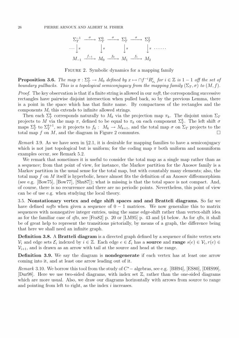
Figure 2. Symbolic dynamics for a mapping family
Proposition 3.6. The map π : Σ0T → M0 defined by x 7→ ∩f−iRi
xifor i ∈ Z is 1− 1 off the set of
boundary pullbacks. This is a topological semiconjugacy from the mapping family (ΣT , σ) to (M, f).
Proof. The key observation is that if a finite string is allowed in our nsft, the corresponding successiverectangles have pairwise disjoint intersection when pulled back, so by the previous Lemma, thereis a point in the space which has that finite name. By compactness of the rectangles and thecomponents Mi this extends to infinite allowed strings.
Then each ΣkT corresponds naturally to Mk via the projection map πk. The disjoint union ΣT
projects to M via the map π, defined to be equal to πk on each component ΣkT . The left shift σ
maps ΣkT to Σk+1
T , so it projects to fk : Mk → Mk+1, and the total map σ on ΣT projects to thetotal map f on M , and the diagram in Figure 2 commutes.
Remark 3.9. As we have seen in §2.1, it is desirable for mapping families to have a semiconjugacywhich is not just topological but is uniform; for the coding map π both uniform and nonuniformexamples occur, see Remark 5.2.
We remark that sometimes it is useful to consider the total map as a single map rather than asa sequence; from that point of view, for instance, the Markov partition for the Anosov family is aMarkov partition in the usual sense for the total map, but with countably many elements; also, thetotal map f on M itself is hyperbolic, hence almost fits the definition of an Anosov diffeomorphism(see e.g. [Bow75], [Bow77], [Shu87]); what is missing is that the total space is not compact. And,of course, there is no recurremce and there are no periodic points. Nevertheless, this point of viewcan be of use e.g. when studying the local theory.
3.5. Nonstationary vertex and edge shift spaces and and Bratteli diagrams. So far wehave defined nsfts when given a sequence of 0 − 1 matrices. We now generalize this to matrixsequences with nonnegative integer entries, using the same edge-shift rather than vertex-shift ideaas for the familiar case of sfts, see [Fra82] p. 20 or [LM95] p. 43 and §4 below. As for sfts, it shallbe of great help to represent the transitions pictorially, by means of a graph, the difference beingthat here we shall need an infinite graph.
Definition 3.8. A Bratteli diagram is a directed graph defined by a sequence of finite vertex setsVi and edge sets Ei indexed by i ∈ Z. Each edge e ∈ Ei has a source and range s(e) ∈ Vi, r(e) ∈Vi+1, and is drawn as an arrow with tail at the source and head at the range.
Definition 3.9. We say the diagram is nondegenerate if each vertex has at least one arrowcoming into it, and at least one arrow leading out of it.
Remark 3.10. We borrow this tool from the study of C∗− algebras, see e.g. [BH94], [ES80], [DHS99],[Dur98]. Here we use two-sided diagrams, with index set Z, rather than the one-sided diagramswhich are more usual. Also, we draw our diagrams horizontally with arrows from source to rangeand pointing from left to right, as the index i increases.

ANOSOV FAMILIES, RENORMALIZATION AND NONSTATIONARY SUBSHIFTS 27
We now describe the edge and vertex labels and associated matrix sequences.
Definition 3.10. First we identify the vertex set Vi with an ordered alphabet Ai = 0, . . . , ai−1;the resulting Bratteli diagram is the vertex-labelled diagram. We associate to the diagram asequence of (ai+1)× (ai) matrices (Fi)i∈Z with nonnegative integer entries by setting the mlth entryof Fi equal to k iff there are k edges connecting vertex l in Vi to vertex m in Vi+1 (and to be 0 ifthere are no such edges).
We say the diagram is single-edged iff there is at most one edge from a given source to a givenrange, or equivalently, iff the matrices Fi have entries 0 or 1.
For the second, we identify the edge set Ei with an ordered alphabet Ai. This gives an edge-labelled diagram. We define a sequence (Ti) of matrices by taking the mlth entry of Ti to be 1 iffthe edge m in Ei+1 follows the edge l in Ei, and otherwise to be 0.
Proposition 3.7. In each case, the diagram determines and is determined by the matrix sequence(Fi), which have nonnegative integer entries for the vertex labels and which always have 0−1 entriesfor the edge labels.
Remark 3.11. The specific matrix sequence is defined in each case by the order on the alphabet,corresponding to ordering the vertices or edges respectively.
As for nsfts, here we have adopted the column vector convention when defining the matrices.
An nsft corresponds to a sequence of 0−1 matrices. If the diagram happens to have single edges,therefore, there are two natural ways to define a sequence of 0−1 matrices and hence an associatednsft, by labelling the vertices or the edges.
Definition 3.11. Given a Bratteli diagram with edge labels, we call the nsft defined by the 0− 1sequence (Fi) the edge-shift space of the diagram. If it is a vertex-labelled and single-edgeddiagram, we we call the resulting nsft the vertex-shift space of the diagram.
Proposition 3.8. Two nondegenerate Bratteli diagrams determine the same edge shifts iff they areequal; for single-edged diagrams the same holds for the vertex shifts.
Proof. This is just like the proof of Proposition 3.4.
Remark 3.12. Given a vertex-labelled diagram with single edges, there is a natural choice for namingthe edges: if an edge e connects symbols s(e) = i and r(e) = j, then this edge is named ij; thesecan then be ordered lexicographically, producing an edge-labelled diagram. This is illustrated inFigures 3, 4, where we have started with the vertex-labelled Bratteli diagram corresponding to thesequence [
1 01 1
]for i even;
[1 10 1
]for i odd
and where the vertices are listed in increasing order from top to bottom.
The edge-labelled diagram defines an nsft, the additive golden shift, which in turn gives a newvertex-labelled diagram, see Figure 5. Symbolically, this construction (the new nsft produced bythe change of symbols from vertices to edges) has this description:
Definition 3.12. A two-block code of an nsft is the new nsft produced by taking as the alphabetallowed words of length two, with the inherited transition rules.
As in the case of sfts, see Proposition 3.2 of [Fra82], we have:
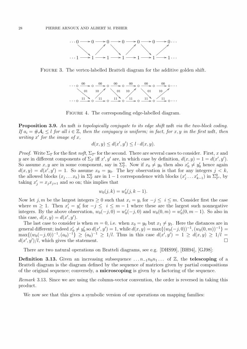
28 PIERRE ARNOUX AND ALBERT M. FISHER
· · · 0 //
!!CCCCCCCC 0 // 0 //
======= 0 // 0 //
======= 0 // 0 · · ·
· · · 1 // 1 //
@@1 // 1 //
@@1 // 1 //
==1 · · ·
Figure 3. The vertex-labelled Bratteli diagram for the additive golden shift.
· · · 00 //
01
""EEEEEEEE 00 // 00 //
01
@@@@@@@ 00 // 00 //
01
@@@@@@@ 00 // · · ·
· · · 11 // 11 //
10??~~~~~~~ 11 // 11 //
10??~~~~~~~ 11 // 11 //
10<<yyyyyyyy · · ·
Figure 4. The corresponding edge-labelled diagram.
Proposition 3.9. An nsft is topologically conjugate to its edge shift nsft via the two-block coding.If ai = #Ai ≤ l for all i ∈ Z, then the conjugacy is uniform; in fact, for x, y in the first nsft, thenwriting x′ for the image of x,
d(x, y) ≤ d(x′, y′) ≤ l · d(x, y).
Proof. Write ΣT for the first nsft, ΣT ′ for the second. There are several cases to consider. First, x andy are in different components of ΣT iff x′, y′ are, in which case by definition, d(x, y) = 1 = d(x′, y′).So assume x, y are in some component, say in Σ0
T . Now if x0 6= y0 then also x′0 6= y′0 hence againd(x, y) = d(x′, y′) = 1. So assume x0 = y0. The key observation is that for any integers j < k,the allowed blocks (xj . . . xk) in Σ0
T are in 1− 1 correspondence with blocks (x′j . . . x′k−1) in Σ0
T ′ , bytaking x′j = xjxj+1 and so on; this implies that
w0(j, k) = w′0(j, k − 1).
Now let j,m be the largest integers ≥ 0 such that xi = yi for −j ≤ i ≤ m. Consider first the casewhere m ≥ 1. Then x′i = y′i for −j ≤ i ≤ m − 1 where these are the largest such nonnegativeintegers. By the above observation, w0(−j, 0) = w′0(−j, 0) and w0(0,m) = w′0(0,m− 1). So also inthis case, d(x, y) = d(x′, y′).
The last case to consider is when m = 0, i.e. when x0 = y0 but x1 6= y1. Here the distances are ingeneral different; indeed x′0 6= y′0 so d(x′, y′) = 1, while d(x, y) = max(w0(−j, 0))−1, (w0(0,m))−1 =max(w0(−j, 0))−1, (a0)−1 ≥ (a0)−1 ≥ 1/l. Thus in this case d(x′, y′) = 1 ≥ d(x, y) ≥ 1/l =d(x′, y′)/l, which gives the statement.
There are two natural operations on Bratteli diagrams, see e.g. [DHS99], [BH94], [GJ98]:
Definition 3.13. Given an increasing subsequence . . . n−1n0n1 . . . of Z, the telescoping of aBratteli diagram is the diagram defined by the sequence of matrices given by partial compositionsof the original sequence; conversely, a microscoping is given by a factoring of the sequence.
Remark 3.13. Since we are using the column-vector convention, the order is reversed in taking thisproduct.
We now see that this gives a symbolic version of our operations on mapping families:

ANOSOV FAMILIES, RENORMALIZATION AND NONSTATIONARY SUBSHIFTS 29
· · · 00 // 00 //
!!BBBBBBBB 00 // 00 //
##GGGGGGGG 00 · · ·
· · · 01 //
##GGGGGGGG 10 //
>>||||||||01 //
!!BBBBBBBB 10 //
;;wwwwwwww10 · · ·
· · · 11 //
;;wwwwwwww11 // 11 //
>>||||||||11 // 11 · · ·
Figure 5. The vertex-labelled diagram which gives the same nsft as Figure 4, andwhich is a two-block code of Figure 3.
· · · 0 2 //
!!CCCCCCCC 02 //
======= 02 //
======= 02 //
======= 02 //
======= 02 //
!!CCCCCCCC 0 · · ·
· · · 1 //
==1 //
@@1 //
@@1 //
@@1 //
@@1 //
==1 · · ·
Figure 6. Telescoped diagram corresponding to the gathering along even times ofthe additive golden shift, with number of edges indicated when > 1.
· · · 0 000
010//
110 !!CCCCCCCC 0000
010//
110 ======= 0000
010//
110 ======= 0000
010//
110 ======= 0000
010//
110 ======= 0000
010//
110 !!CCCCCCCC 0 · · ·
· · · 1111
//011
==1
111//
011
@@1
111//
011
@@1
111//
011
@@1
111//
011
@@1
111//
011
==1 · · ·
Figure 7. The same diagram with its additive edge labels; the upper two labels arefor two edges.
· · · 0 //
!!CCCCCCCC 0 //
======= 0 //
======= 0 //
======= 0 //
======= 0 //
!!CCCCCCCC 0 · · ·
· · · 1
==1
@@1
@@1
@@1
@@1
==1 · · ·
Figure 8. A second diagram which telescopes to that of Figure 6; now the edgelabels are different from those of Figure 7.
Proposition 3.10. Given a generating Markov partition P of a mapping family (M, f), the op-erations of gathering and of dispersal via the insertion of identity maps for the family correspondto telescoping and microscoping of the Bratteli edge diagram. That is, the nsft for the augmented
trivial gathering of P, which is the partition P defined by Pi = Pi∨Pi+1, is equal to the nsft for theedge labeling of the Bratteli diagram associated to P; and telescoping this diagram along an increas-ing subsequence ni gives an edge-labelled diagram whose nsft is identical to that for the augmentedgathered partition taken along that subsequence.
The proof is immediate from the definitions; See Remark 3.1.

30 PIERRE ARNOUX AND ALBERT M. FISHER
3.6. The (2×2) case: additive sequences and canonical labelings. Now we restrict attentionto Bratteli diagrams with two vertices, i.e. those given by a sequence of (2×2) nonnegative matrices.This is the case we shall need for the rest of the paper.
We noted above that for a single-edged Bratteli diagram, a vertex labelling gives natural labelsfor the edges. In general for multiple edges, there is no canonical way to pass from vertex to edgelabels; however as we shall see, in the (2 × 2) case this is in fact possible. This labelling will beneeded later, in Theorem 5.6.
We recall that SL(2,Z) is the group of (2×2) matrices with integer entries and with determinant1. We shall write SL(2,N) for the subsemigroup whose entries are all ≥ 0.
The next lemma is well-known and we do not know the proper attribution; we learned this simpleproof a long time ago, perhaps from Rauzy.
Lemma 3.11. SL(2,N) is the free semigroup generated by the additive generators
M =
[1 01 1
]and N =
[1 10 1
].
Proof. We note that the identity I =
[1 00 1
]is included here as I = M0 = N0. Let A ∈ SL(2,N),
with A =
[a bc d
]. We claim that if A 6= I, then either the first column is ≥ the second, in the sense
that a ≥ b and c ≥ d, or the reverse.If both of these conditions fail then either a > b and c < d or the reverse. However the reverse
(b < a and d > c) cannot happen as this would imply that bc > ad so ad−bc < 0, but by assumptionthe determinant is one.
Since therefore a > b and c < d, we have: a ≥ b+ 1 and d ≥ c+ 1 so the determinant is:
ad− bc ≥ (b+ 1)(c+ 1)− bc = bc+ b+ c+ 1− bc = b+ c+ 1.
Since detA = 1, we have b and c = 0 in which case A = I, as claimed.Now we show that A ∈ SL(2,N) can be factored as a product of nonnegative powers of M and
N . Writing A = A0, if A0 6= I then remove the smaller column from the larger to form A1. Thisamounts to writing
A1 = A0M−1 or A1 = A0N
−1;
note that the new matrix A1 is still in SL(2,N). If A1 again has one column larger than the otherthen we continue, producing a sequence A0, A1, . . . , An. This process terminates with a matrix Anwith determinant one and which has neither column larger than the other. So as shown above,An = I. Thus, reversing the process, we have factored A as a product of nonnegative powers of Mand N .
We have proved a little more: the preceding argument shows that an element of SL(2,N) whichis not the identity can be factored either as A = A1N or as A = A1M , but not both. Therefore thedecomposition of A in terms of M and N is unique, and this implies that there can be no nontrivialrelations in the semigroup SL(2,N); hence it is free.
Remark 3.14. What the proof has shown is that there is a unique way to get to a given positivematrix with determinant one by starting with I, adding one column to the other and repeating theoperation. From a different point of view, this is exactly the construction of the Farey tree.

ANOSOV FAMILIES, RENORMALIZATION AND NONSTATIONARY SUBSHIFTS 31
Of course one would like such a theorem for the (3×3) case, but there is no hope of such a simplestructure, as it is known that SL+(3,Z) is neither finitely generated nor free. (Joel Rivat, privatecommunication).
A sequence (Ai)i∈Z such that each matrix either equals one of the additive generators M,N weshall call an additive sequence. We call the Bratteli diagram defined by such a sequence anadditive diagram.
Given a sequence (Fi), from SL(2,N), consider the Bratteli diagram determined by (Fi); thusthere are two symbols 0 and 1 and the matrix entries specify the number of edges. In general fora multiple-edged diagram there is no natural way to label the edges. However in this case we havesuch a way, given by the Lemma:
Corollary 3.12.(i) A sequence (Fi) with Fi ∈ SL(2,N) uniquely determines an additive sequence (Aj) such thatF0 = An · · ·A1A0, F1 = An+k · · ·An+1 and so on for Fi with i ∈ Z.(ii) Fixing the location of time 0, there is a unique additive diagram, the additive microscoping,which telescopes to the Bratteli diagram for (Fi). The gathered labels on the edges of this diagramspecify the paths of the additive microscoping.
We call the resulting canonical edge labels for the diagram its additive labels. See Fig. 3.5.Thus, given a sequence (Fi) of (2 × 2) matrices with nonnegative integer entries, in view of
Corollary 3.12, we can associate an nsft to (Fi) of that special type in a canonical way:
Definition 3.14. Given sequence (Fi) with Fi ∈ SL(2,N), we define ΣF to be the nsft determinedup to by gathering the nsft determined by the additive factorization, with its time-zero partition,and with the gathered partition elements labelled accordingly, and ordered in some chosen way.
4. The multiplicative family.
For the rest of the paper we focus on certain Anosov families on the two-torus, given by a sequenceof (2× 2) matrices. As we will see, the corresponding codings will also come from (2× 2) matrices,as studied in §3.6. Our main example is this:
Definition 4.1. Given the choice of a sequence 〈n〉 ≡ (. . . n−1n0n1 . . . ) ∈ Π+∞−∞N∗ for N∗ =
1, 2, . . . and a parity p ∈ +,−, the square torus version of the multiplicative fam-ily determined by 〈n〉 and p is the mapping family (M, f) = (Mi, fi) along a sequence of two-tori,defined as follows.
We take first the case of parity (+). We set
Ai =
[1 0ni 1
]for i even;
[1 ni0 1
]for i odd.
For each i ∈ Z, let Mi = R2/Z2, with the standard Euclidean metric and thought of as columnvectors.
We define fi : Mi →Mi+1 to be the function given by left multiplication by Ai; that is, for (x, y)in Mi = R2/Z2,
fi :
[xy
]7→ Ai
[xy
].
For parity (−) the transposes are used instead.

32 PIERRE ARNOUX AND ALBERT M. FISHER
We will show (M, f) is an Anosov family, by describing the expanding and contracting eigendi-rections and eigenvalues explicitly. Changing to eigencoordinates will give a second version of themultiplicative family, which is boundedly conjugate to the square torus version; see Proposition 4.3.
We shall use this terminology: an individual matrix Ai as above has parity (+), (−) if it is lower,respectively upper, triangular; thus the sequence (Ai)i∈Z has parity (+) exactly when each of thematrices at even times has parity (+).
From the sequence (Ai) we will define a sequence of matrices (Bi), the columns of which will give
our eigenvectors. These matrices will be in a set B0 = B0,+ ∪ B0,− ⊆ SL(2,R) with B =
[a c−b d
]satisfying the conditions:
(1) (i): a, b, c, d ≥ 0(ii): detB = 1(iii): for B ∈ B0,+, 0 < a < 1 ≤ b = 1 and d < c
for B ∈ B0,−, 0 < b < 1 ≤ a = 1 and c < d.
We say B ∈ B0 has parity (+) or (−) when it is in B+ or B− respectively.Given a sequence of integers m0,m1, . . . with mi ≥ 1, we shall use this notation for the (multi-
plicative) continued fraction:
[m] = [m0m1 . . . ] =1
m0 +1
m1 + · · ·The correspondence (mi)i∈N 7→ [m] defines a bijection from Π+∞
0 N∗ and the set of irrationals in(0, 1).
Proposition 4.1. Given a choice of 〈n〉 ∈ Π+∞−∞N∗ and parity (+) or (−), then the mapping family
(M, f) as defined above is an Anosov family. The eigenspaces Esi and Eu
i of Mi = R2/Z2 are
spanned by vectors vsi =
[ai−bi
], vui =
[cidi
], with eigenvalue sequences (λ−1
i ) < 1 and (λi) > 1
respectively, where these are defined by the condition aidi + cibi = 1 together with:
for Ai with parity (+) : ai = [nini+1 . . . ], bi = 1,dici
= [ni−1ni−2 . . . ], and λi =1
ai
for Ai with parity (−) : bi = [nini+1 . . . ], ai = 1,cidi
= [ni−1ni−2 . . . ], and λi =1
biProof. We began with the sequence 〈n〉, parity p = + or (−), and the associated sequence ofmatrices (Ai). From the positive real numbers ai, bi, ci, di determined by this as in the statement ofthe Proposition, we define
Bi =
[ai ci−bi di
]Since aidi + cibi = 1, we have detBi = 1. Thus, from the sequence (Ai), or equivalently from〈n〉 ∈ Π+∞
−∞N∗ together with a choice of parity p we have defined a sequence of matrices Bi ∈ B0,with parity of Bi the same as that for Ai.
Next we define the diagonal matrices
Di =
[λi 00 λ−1
i
]

ANOSOV FAMILIES, RENORMALIZATION AND NONSTATIONARY SUBSHIFTS 33
Figure 9. Two fundamental domains for the lattice, in eigencoordinates: the paral-lelogram and the two-box partition R0. The picture has been rotated counterclock-wise by 90 for convenience. Thus in the above picture, the horizontal axis gives theexpanding direction.
We claim that the sequences Ai, Bi, Di are related as follows:
AiBiDi = Bi+1.
This will finish the proof, since the vectors vsi , vui are the columns of Bi, and we have from the above
equation that
Aivsi = AiBi
[10
]= Bi+1D
−1i
[10
]= λ−1
0 vsi+1
as claimed.To verify the claim is immediate; we check this for i = 0 and parity (+). We have
A0B0 =
[a0 c0
−(b0 − n0a0) d0 + n0c0
](2)
and so:
b1 =b1
a1
≡ [n1n2 . . . ] =1
a0
− n0 =b0 − n0a0
a0
= λ0(b0 − n0a0), (3)
and similarly for the other matrix entries. Hence indeed A0B0D0 = B1, as claimed.
We use the above diagonalization to define a second mapping family, which expresses the multi-plicative family in eigencoordinates.
We write Ni ≡ R2/Λi where Λi is the lattice spanned by the columns of B−1i , with the Euclidean
metric inherited from R2, and define maps gi : Ni → Ni+1 by
gi :
[xy
]7→ D−1
i
[xy
].
We call (N, g) the eigencoordinate version of the multiplicative family (M, f).

34 PIERRE ARNOUX AND ALBERT M. FISHER
Lemma 4.2. For a matrix in B0, the row vectors have length in the interval (1/2,√
2) and theangle θ between them satisfies sin(θ) ≥ 1/2.
Proof. Consider the case of parity (+). From the conditions 1(i), (ii), (iii) which define B0, we haveb = 1 and a, c, d ≤ 1. Hence the vectors (−b, d) and (a, c) have length no more than
√2.
Writing v = (−b, d) and w = (a, c), we know the parallelogram spanned by v, w has area 1, so1 = ||v|| · ||w|| sin(θ) where θ is the angle between them. So from the length estimate, sin(θ) =1/(||v|| · ||w||) ≥ 1/2 as claimed.
Note: these estimates are not optimal, but we need only rough bounds.
Proposition 4.3. The Anosov families (M, f) and (N, g) are boundedly conjugate via the maps
hi : Mi → Ni defined by [xy
]7→ B−1
i
[xy
].
For (N, g), the eigenvector sequences
wsi =
[10
]and wui =
[01
]have the same eigenvalues, (λ−1
i ) and (λi) respectively.
Proof. From the formulaB0 7→ A0B0D0 = B1
we have the commutative diagram
M0A0−−−→ M1
A1−−−→ M2A2−−−→ M3
······xB0
xB1
xB2
xB3 · · · · · ·
N0
D−10−−−→ N1
D−11−−−→ N2
D−12−−−→ N3
for the action on column vectors, and D−1i is the diagonalization of Ai with respect to the eigenbases.
The conjugacy of the families is then simply left multiplication of column vectors by B−1i . This
shows the conjugacy on R2. It remains to check that Ni maps to Ni+1. It is enough to show thatD−1i (Λi) = Λi+1. Taking the inverse of the formula AiBiDi = Bi+1 we have
B−1i+1 = D−1
i B−1i A−1
i ;
now since A−1i ∈ SL(2,Z), right multiplication by this gives a matrix whose columns span the same
lattice in R2, as we wanted.The statement about eigenvectors follows immediately from the diagonalization.Now we show the conjugacy is bounded. From Lemma 4.2, the ellipses which are the images of
the unit ball by the matrices Bi acting on row vectors have a uniformly bounded inner and outerradius. Hence the same is true for the matrices B−1
i acting on columns, as the columns of B−1i are
a rotation by π/2 of the rows of Bi. Thus by Lemma 2.9, this is a bounded conjugacy.
Remark 4.1. The above conjugacy, while bounded, is not an isometry. Indeed, for the family (M, f)the metric on each torus Mi is the same, while the tori Ni in general are not even isometric, asfor instance the length of the minimum closed geodesic will change. For Mi the metric has beenchosen so that the standard basis vectors are orthogonal and have length 1, while the eigenvectors
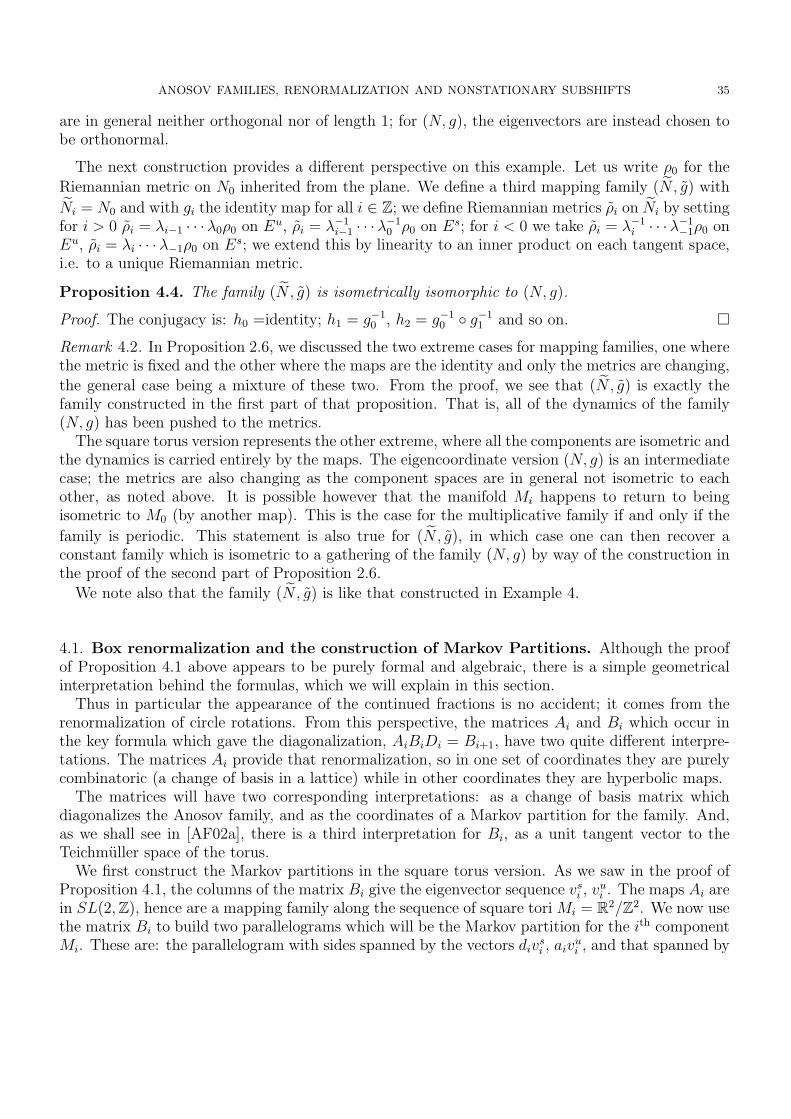
ANOSOV FAMILIES, RENORMALIZATION AND NONSTATIONARY SUBSHIFTS 35
are in general neither orthogonal nor of length 1; for (N, g), the eigenvectors are instead chosen tobe orthonormal.
The next construction provides a different perspective on this example. Let us write ρ0 for the
Riemannian metric on N0 inherited from the plane. We define a third mapping family (N , g) with
Ni = N0 and with gi the identity map for all i ∈ Z; we define Riemannian metrics ρi on Ni by settingfor i > 0 ρi = λi−1 · · ·λ0ρ0 on Eu, ρi = λ−1
i−1 · · ·λ−10 ρ0 on Es; for i < 0 we take ρi = λ−1
i · · ·λ−1−1ρ0 on
Eu, ρi = λi · · ·λ−1ρ0 on Es; we extend this by linearity to an inner product on each tangent space,i.e. to a unique Riemannian metric.
Proposition 4.4. The family (N , g) is isometrically isomorphic to (N, g).
Proof. The conjugacy is: h0 =identity; h1 = g−10 , h2 = g−1
0 g−11 and so on.
Remark 4.2. In Proposition 2.6, we discussed the two extreme cases for mapping families, one wherethe metric is fixed and the other where the maps are the identity and only the metrics are changing,
the general case being a mixture of these two. From the proof, we see that (N , g) is exactly thefamily constructed in the first part of that proposition. That is, all of the dynamics of the family(N, g) has been pushed to the metrics.
The square torus version represents the other extreme, where all the components are isometric andthe dynamics is carried entirely by the maps. The eigencoordinate version (N, g) is an intermediatecase; the metrics are also changing as the component spaces are in general not isometric to eachother, as noted above. It is possible however that the manifold Mi happens to return to beingisometric to M0 (by another map). This is the case for the multiplicative family if and only if the
family is periodic. This statement is also true for (N , g), in which case one can then recover aconstant family which is isometric to a gathering of the family (N, g) by way of the construction inthe proof of the second part of Proposition 2.6.
We note also that the family (N , g) is like that constructed in Example 4.
4.1. Box renormalization and the construction of Markov Partitions. Although the proofof Proposition 4.1 above appears to be purely formal and algebraic, there is a simple geometricalinterpretation behind the formulas, which we will explain in this section.
Thus in particular the appearance of the continued fractions is no accident; it comes from therenormalization of circle rotations. From this perspective, the matrices Ai and Bi which occur inthe key formula which gave the diagonalization, AiBiDi = Bi+1, have two quite different interpre-tations. The matrices Ai provide that renormalization, so in one set of coordinates they are purelycombinatoric (a change of basis in a lattice) while in other coordinates they are hyperbolic maps.
The matrices will have two corresponding interpretations: as a change of basis matrix whichdiagonalizes the Anosov family, and as the coordinates of a Markov partition for the family. And,as we shall see in [AF02a], there is a third interpretation for Bi, as a unit tangent vector to theTeichmuller space of the torus.
We first construct the Markov partitions in the square torus version. As we saw in the proof ofProposition 4.1, the columns of the matrix Bi give the eigenvector sequence vsi , v
ui . The maps Ai are
in SL(2,Z), hence are a mapping family along the sequence of square tori Mi = R2/Z2. We now usethe matrix Bi to build two parallelograms which will be the Markov partition for the ith componentMi. These are: the parallelogram with sides spanned by the vectors div
si , aiv
ui , and that spanned by

36 PIERRE ARNOUX AND ALBERT M. FISHER
x,y
-l0
h0
l1
h1
Figure 10. The box pair in eigencoordinates, for i with parity (+): the row vectorsof Bi are the coordinates of the vectors which generate the parallelogram lattice. Thepicture has been rotated 90 counterclockwise. For parity (−), this picture is reflectedin the vertical axis. In both cases, the left box is R1
i and the right box is R0i .
civsi , −bivui . Note that the union of these two parallelograms gives a second fundamental domain for
the lattice Z2 acting on R2; thus they partition the torus. Indeed the condition detBi = 1 impliesthat the areas of the parallelograms aidi · det(Bi), | − bici| · det(Bi) add up to one.
See Fig. 1 for the simplest example (with ni = 1 for all i); in this case the eigendirections areorthogonal, as noted in §3.2, and moreover the boxes happen to be square, as is easily calculatedfrom the above formulas.
In the eigencoordinates, the first parallelogram is spanned by the vectors ciwsi , −biwui , the second
by diwsi , aiw
ui .
The parallelograms have become rectangles as the eigenvectors are now orthogonal. We call theserectangles boxes and write Ri = R0
i , R1i for the resulting partition of Ni ≡ R2/ΛBi
.Note that in the eigencoordinates the lattice which defines the torus has become a parallelogram
lattice. The vectors (d, b) and (−c, a) generate this lattice; these are the columns of B−1i .
It will be convenient to rotate the eigencoordinates counterclockwise by 90 for the illustrations(see Figures 9, 10, 11, 12). Then the vector wui is (−1, 0) after rotation, while wsi is (0, 1), so therectangle R0
i is the right-hand box; changing the orientation of the horizontal axis to agree with thestandard coordinates, this box has as base the interval [0, bi] on the horizontal axis and height theinterval [0, ci] on the vertical axis; the box R1
i has base [−ai, 0] and height [0, di].Therefore the boundary of the partition Ri is, in the rotated coordinates, the segment [−ai, bi]
on the x-axis union the segment [0,maxci, di] on the y-axis. See Figure 10.Note that in this picture, our choice of bi = 1, for parity (+) (hence for i even) has this geometrical
meaning: the larger of the two boxes (with respect to both height and width) is on the right, whilefor parity (−) this switches.
In the proof of Proposition 4.1, we encountered the formula
A0B0D0 = B1.

ANOSOV FAMILIES, RENORMALIZATION AND NONSTATIONARY SUBSHIFTS 37
Figure 11. Box renormalization, in the eigencoordinates, showing two points equiv-alent under the lattice action, after rotation of the coordinates by 90 counterclock-wise.
This formula has the following geometrical interpretation. Consider the related operation
B0 7→ A0B0 = B1D−10 .
We use the new matrix A0B0 to define a new pair of boxes on the same torus, N0 ≡ R2/ΛB0 , in thesame way as just described for B0. We call this procedure of passing from one pair of boxes to thenext box renormalization. It has a simple algorithmic description, as we shall show:
Proposition 4.5. Consider the multiplicative family given by a choice of 〈n〉 and parity. Inthe eigencoordinate representation (N, g), the pullback of the partition Ri on Ni to the torusN0 ≡ R2/ΛB0 gives the sequence of partitions defined as above from the matrices B0, A0B0 =B1D
−10 , A1A0B0 = B2D
−10 D−1
1 , . . . . Equivalently, the sequence of box pairs is given by box renor-malization: first, remove as many copies as possible of the smaller base interval, e.g. for parity (+)that with length a0 from the right side of the larger, with length b0 = 1. Next, cut the larger boxinto corresponding pieces and restack these parts above the smaller one, producing the second pairof boxes. For the third pair, begin with the right box, as the parity has changed and that is nowshorter. The partition sequence Ri is a Markov partition sequence for the mapping family (N, g).
Proof. Note that the number of copies of the interval of length a0 removed is the greatest integer[b0a0
]=[
1a0
]= n0. And so from equation (2) the box renormalization produces a new pair of boxes,
whose sides have new relative lengths given by the matrix A0B0.
4.2. Producing a generator: the Adler-Weiss method. This describes a partition sequencewith the Markov property. However the Rk do not generate, i.e. separate points. To produce agenerator from R we employ a method of Adler and Weiss [AW70]. We define Pk to be the partition
consisting of the closures of the connected components ofRk∨g−1
k (Rk+1). As in §3.1, P∨Q denotes
the join of two partitions. (ByR we mean the union of the interiors of the elements of the partition
R.) We need to take interiors here as we want the new boundary to be the same as the old, andnot to have two pieces accidentally glued together.) We shall call Pk the connected-componentpartition for the multiplicative family.

38 PIERRE ARNOUX AND ALBERT M. FISHER
Figure 12. From left to right: two-box partition R0 with b0 = 1, cut to give gen-erating partition P0 with n0 + 1 elements labelled, reading from left to right, 1111,0000, 0001, 0011, and 0111 (see the end of §4) ; rescaling by the diagonal matrix soa1 = 1; stacking to get b1, c1, d1 and new two-box partition R1. The last two picturesoverlap, and connected components of R1 join the rescaled R0 give the rescaled P0.
Proposition 4.6. The connected-component partition P = (Pk)k∈Z is a generating Markov partitionsequence for the multiplicative family (N, g). This passes by conjugacy over to a generating Markovpartition sequence for the square-torus multiplicative family (M, f). For a chosen parity (+) or (−),the partition of any given component varies continuously with respect to the Hausdorff metric, withrespect to 〈n〉 ∈ Π+∞
−∞N∗.
Proof. The boundary of P0 now consists of the two segments [−a0, b0] and [0, d0 + n0c0] = [0, λ0b1].Therefore it satisfies the Markov property, as above. Now the elements of the partition (g−n)nPn ∨. . .P0 ∨ · · · ∨ (gn)−nPn are also connected sets. Hence their diameters → 0 as n → ∞, so thereis at most one point in a given infinite intersection of the interiors. Continuity of the partitionboundaries is immediate from the formula for the coordinates of the two boxes, and this passes overto the connected components.
In the next section we will describe another way to construct this generator, which automaticallyleads us to natural labels for the partition elements.
5. An extension of theorems of Adler and Manning to mapping families
Recall that SL(2,R), SL(2,Z) are the the groups of (2 × 2) matrices with real (respectivelyinteger) subgroups with determinant 1. An element A ∈ SL(2,Z) induces an orientation-preservingautomorphism of the two-torus (thought of as the factor group R2/Z2) by left mutiplication ofcolumn vectors. Such an automorphism is hyperbolic when it has two eigenvalues λ, λ−1 with λ > 1.
In [Adl98] Adler proves a theorem which includes the following: for any orientation-preserving(2× 2) hyperbolic toral automorphism A with nonnegative entries there exists a Markov partitionsuch that the map codes as an edge shift using exactly the same matrix. Thus, when
A =
[p qr s
],
there is a generating partition of the torus with p + q + r + s elements, which is coded as an edgeshift on two vertices, labelled 0 and 1, such that there are (in the column vector convention) pedges from 0 to itself, q from 1 to 0 and so on; that is, the toral automorphism is coded as an sftwith edges for symbols, where one symbol can follow another exactly when that edge can follow theother edge in the graph.
Anthony Manning proved a similar result independently. See [Man02] and Remark 5.3.
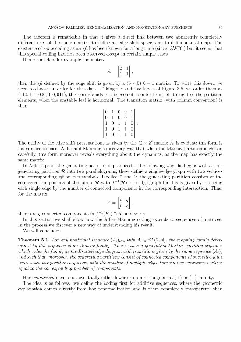
ANOSOV FAMILIES, RENORMALIZATION AND NONSTATIONARY SUBSHIFTS 39
The theorem is remarkable in that it gives a direct link between two apparently completelydifferent uses of the same matrix: to define an edge shift space, and to define a toral map. Theexistence of some coding as an sft has been known for a long time (since [AW70]) but it seems thatthis special coding had not been observed except in certain simple cases.
If one considers for example the matrix
A =
[2 11 1
],
then the sft defined by the edge shift is given by a (5 × 5) 0 − 1 matrix. To write this down, weneed to choose an order for the edges. Taking the additive labels of Figure 3.5, we order them as(110, 111, 000, 010, 011); this corresponds to the geometric order from left to right of the partitionelements, when the unstable leaf is horizontal. The transition matrix (with column convention) isthen
0 1 0 0 10 1 0 0 11 0 1 1 01 0 1 1 01 0 1 1 0
.The utility of the edge shift presentation, as given by the (2× 2) matrix A, is evident; this form ismuch more concise. Adler and Manning’s discovery was that when the Markov partition is chosencarefully, this form moreover reveals everything about the dynamics, as the map has exactly thesame matrix.
In Adler’s proof the generating partition is produced is the following way: he begins with a non-generating partition R into two parallelograms; these define a single-edge graph with two verticesand corresponding sft on two symbols, labelled 0 and 1; the generating partition consists of theconnected components of the join of R with f−1(R); the edge graph for this is given by replacingeach single edge by the number of connected components in the corresponding intersection. Thus,for the matrix
A =
[p qr s
],
there are q connected components in f−1(R0) ∩R1 and so on.In this section we shall show how the Adler-Manning coding extends to sequences of matrices.
In the process we discover a new way of understanding his result.We will conclude:
Theorem 5.1. For any nontrivial sequence (Ai)i∈Z with Ai ∈ SL(2,N), the mapping family deter-mined by this sequence is an Anosov family. There exists a generating Markov partition sequencewhich codes the family as the Bratteli edge diagram with transitions given by the same sequence (Ai),and such that, moreover, the generating partitions consist of connected components of sucessive joinsfrom a two-box partition sequence, with the number of multiple edges between two successive verticesequal to the corresponding number of components.
Here nontrivial means not eventually either lower or upper triangular at (+) or (−) infinity.The idea is as follows: we define the coding first for additive sequences, where the geometric
explanation comes directly from box renormalization and is there completely transparent; then

40 PIERRE ARNOUX AND ALBERT M. FISHER
we show that these codings behave well with respect to the operation of gathering, and that con-nected components correspond exactly to different names along the additive factorization. The finalstep is to remember from Lemma 3.11 that any sequence of nonnegative matrices has a canonicalfactorization in terms of the additive generators, allowing us to apply the previous result.
5.1. Additive and linear families. We call a sequence Fi ∈ SL(2,N), for i ∈ Z, a (nonnegative)linear sequence. A linear sequence defines a mapping familiy by its action on column vectors,with spaces the square torus R2/Z2, i.e. with the standard Euclidean metric inherited from theplane. We call this the linear family determined by (Fi)i∈Z.
Now we treat Example 6 from §2 in detail. When the linear sequence is such that each matrixFi either equals one of the additive generators[
1 01 1
]or
[1 10 1
],
we call this an additive family; we say these generators have parity (+) and (−) respectively. Wesay an additive familiy is nontrivial if the matrices change parity infinitely often at both +∞ and−∞.
Every nontrivial additive family gathers to a multiplicative family, collecting neighboring upperand lower triangular matrices in the obvious way, possibly after a shift to have the change of parityoccur between times −1 and 0. The converse holds also, since of course the mutiplicative familyfactors as powers of the generators, giving a (nontrivial) additive family.
More generally, by Lemma 3.11, any nonnegative linear sequence factors uniquely as an additivefamily, as in part (i) of Corollary 3.12.
(Removing the trivial additive families i.e. the eventually constant sequences corresponds exactlyto removing the rational directions for the stable and unstable foliations, and is a countable set.)
5.2. A Markov Partition and symbolic dynamics for the additive family. We describe nexta Markov partition sequence for a nontrivial additive family. Here we have a generating sequencefrom the outset, without needing to take connected components of joins. This construction willthen give a new way of getting generators for the multiplicative families.
We begin with a sequence 〈n〉 = (. . . n0n1 . . . ) ∈ Π+∞−∞N∗ and assume for simplicity as above that
the additive sequence (Ai) changes parity between coordinates −1 and 0. The additive family then
gathers to the multiplicative family which we shall now write as (Ai).Corresponding to the map
Bi 7→ AiBiDi = Bi+1,
which describes algebraically the operation of multiplicative box renormalization, we now have theequation
Bk 7→ AkBkDk = Bk+1,
which corresponds to the renormalization being done additively, step by step; that is, at each stagei we remove and stack one box, repeating this ni times. The diagonal matrix Dk is defined so as torenormalize the boxes, keeping the largest width always equal to 1.
The generating Markov partitions now are easy to describe: they are for each component Mk
just the pair of boxes. Let us write this partition sequence as Pk; we shall compare this to the
multiplicative partition already defined, which we shall now write as Pk. We have:
Lemma 5.2. The sequence Pk generates for the additive family.

ANOSOV FAMILIES, RENORMALIZATION AND NONSTATIONARY SUBSHIFTS 41
Proof. We give two proofs. The first is direct: note that the intersections of the interiors of thepartition elements after being pulled back by the appropriate maps are always connected, whileclearly the widths (and the heights for negative time) go to 0. Hence they separate points i.e.generate.
The second proof is more abstract: it begins with the generating partition for the multiplicativefamily given in Proposition 4.6. Next, by Lemma 5.4 which follows, this partition, the connectedcomponent partition, is equal to augmented gathered partition; finally, by the converse part ofProposition 3.1, the partition sequence P therefore generates for the additive family.
It turns out that an especially nice symbolic dynamics will result from labelling the two boxes ofPk in the following way:
Theorem 5.3. For the additive family (M, f) given by the additive sequence A = (Ai)i∈Z acting oncolumn vectors, then if we assign to the left box the symbol 1 and to the right-hand box the symbol0, the corresponding nonstationary sft defined by the above coding has for its defining transitionmatrices the same sequence of matrices. That is, the nsft is ΣA.
Proof. Let us suppose that the parity of the additive family given by Ai is (+); thus we have
Ai =
[1 01 1
]. As in Figure 11, the wider box is on the right, and this has label 0; the pullback of
the partition at time i+ 1 meets this exactly in the renormalized boxes defined by the matrix Bi+1,and so the points of box 0 at time i can either be in box 0 or 1 at time i+ 1, while those in box 1
will necessarily next be in box 1. Hence the column transition matrix is
[1 01 1
], exactly the same
matrix.
5.3. Gathering, connected components, and symbolic dynamics. The connection with the
generating partition sequence Pk of Mk, for the multiplicative family, is given by:
Lemma 5.4. For the multiplicative family (M, f), the connected-component partition Pi is theaugmented gathered partition of the partition P, taken along the subsequence of times (ni). Thus,
Pi is equal to the join of the pullbacks to the component Mi = Mniof the (ni + 1) partitions Pk into
two boxes, for ni ≤ k ≤ ni+1.
Proof. This is clear from the definitions; see Figure 12. Thus, e.g. for n0 = 1,
P0 = P0 ∨ (g0)−1(P1)
which has three elements.
In fact something similar is true in much more generality:
Lemma 5.5. Let (Ak) be an additive family, and let Pk be its two-box (generating) partition. Let
(mi) be any increasing subsequence with mi ∈ Z and define A to be the family gathered along that
subsequence of times. Define (Pi) to be the connected-component partition sequence for (mi); that is,
the elements of Pi are the connected components of the join of Pmiwith the pullback of Pmi+1
by the
composed map. Then (Pi) is equal to the augmented gathered partition taken along the subsequence(mi) of the additive partition P.

42 PIERRE ARNOUX AND ALBERT M. FISHER
Proof. We observe that in the eigencoordinate version of the multiplicative family, the boundariesof the two boxes at time mi are formed by a union of two segments in the x and y axes, eachcontaining the point (0, 0) and forming a T shape. Pulling back the corresponding two intervalsfrom the future time mi+1 gives a subinterval of the unstable interval and a segment which containsthe stable interval. We are to show that the connected components of the complement of these fourclosed intervals in the torus is the same as the partition given by the join of all box-pairs for allthe times up to and including time mi+1, which gives the augmented gathered partition. But thetwo pullback segments respectively are contained in and contain all of these in-between pulled backsegments, as they are in the expanding and contracting leaves. Hence no new boundaries are addedin the augmented gathering (it gives exactly the same vertical striping of the two original boxes),verifying the claim.
Remark 5.1. Note that for the additive family, the obvious two-box partition sequence alreadygenerates, with no need to take connected components.
We remark that the additive partition sequence is slightly more efficient than the multiplicative
one. This one sees from the expression in Lemma 5.4; note that in defining Pi there is a bit ofredundancy, as each partition Pk for k = . . . , n0, n0 +n1, . . . gets included twice: this is exactly thedifference between the gathered and augmented gathered partitions of P along the sequence (ni).
The lemma shows the relationship between the connected-component method and augmentedgathering along the additive family, and hence the connection with telescoping of Bratteli diagrams,by Proposition 3.10, leading to the following:
Theorem 5.6. Given (Fi) in SL(2,N), the linear family has a Markov partition which codes it asa Bratteli edge diagram with additive labels determined by the same sequence (Fi).
That is, the unique additive sequence (Aj) determined by the sequence (Fi) from Lemma 3.11serves two purposes: it gives the unique additive dispersal of the family (Fi), and for this dispersal,the two-box partition sequence generates and is coded by the sequence (Aj); microscoping this single-edged diagram gives a multiple-edged diagram on two symbols with additive labels, and with thenumber of edges given by the sequence (Fi). Taking the connected components of pullbacks of thetwo-box partitions for (Fi) gives a generating Markov partition, which is the augmented gatheringof the additive partition taken along that subsequence.
We recall from Definition 3.14 that a (2 × 2) sequence of nonnegative integer matrices (Fi)determines an nsft called ΣF . We write (M, f) for the mapping family on the torus defined by (Fi)acting on columns.
Corollary 5.7. The coding by the nsft ΣF of the linear family (Fi) defines a topological conjugacyπ from the mapping family (ΣF , σ) to the family (M, f).
Remark 5.2. It is natural to ask when this topological conjugacy is in fact uniform (from the wordmetric on the combinatorial space to the Eucldean metric on the torus). One can show that formultiplicative family it is always uniform, in fact is uniformly Lipschitz; for additive families thisis true if and only if the sequence ni is bounded above. Furthermore, uniformity is preserved bygatherings. We shall present these results in a later paper.
Example. Because a positive linear family (Fi) has a unique additive sequence, the elements of thegenerating Markov partition described above inherit natural labels. We describe the labels for thecase of the multiplicative family, see Figure 12. For k even, taking for example k = 0 and n0 = 3, as

ANOSOV FAMILIES, RENORMALIZATION AND NONSTATIONARY SUBSHIFTS 43
in the Figure, we have that the elements of the partition P0, reading from left to right, are labelledas follows: the smaller (leftmost) of the two boxes is labelled 1111, and the larger box is cut intopieces labelled 0000, 0001, 0011, and 0111 respectively; taking e.g. n1 = 3, for the partition P1, withparity reversed, we have that its smaller box, now on the right, is labelled 0000, and 0, 1, 2, 3 arelabelled (from right to left) 1111, 1000, 1100, and 1000. We shall see the usefulness of these labelsin a later paper.
Remark 5.3. In defining shift spaces, one can let the transition matrices act “on columns” as wedo here, or “on rows” (the more usual choice, in Markov chain theory; for Bratteli diagrams,the column convention is often used). Similarly, matrices can be chosen to act on the torus bymultiplying row vectors or columns (the more common convention in dynamical systems theory).Thus, it is usual in dynamics to have a mixture of the conventions. Ordinarily this makes littledifference, but when taking a sequence of matrices, as we do here, making a consistent choice isnotationally important, as otherwise the order of matrix multiplication is reversed. And even for asingle Anosov map, consistency is crucial if one wants to get the nice Adler-Manning-type coding.Thus in Adler [Adl98] the matrices act on the right on row vectors, as shift space are defined inthe usual (row) way. Once we know this result, then an immediate corollary is that if instead thecolumn vector convention is used both for the maps and transitions, one again gets the same matrixfor both; whereas if a mixed convention is chosen, the coding matrix will be the transpose of thatwhich gives the map.
Anthony Manning (personal communication) in the early 1980’s, independently of Adler, discov-ered such a coding of Anosov toral automorphisms, using a mixed convention and thus ending upwith the transpose matrix.
In fact we rediscovered this by accident; unaware of Adler or Manning’s work, and studying thecase of additive families, we had initially used a mixed convention but with switched labels 0 and 1on the boxes. In this case the two operations cancel, yielding exactly the same sequence of matrices.Furthermore this extends to multiplicative families by gathering, providing a nice theorem. Howeverwhen one gathers further-thus mixing parities- then the coding gets hopelessly confused. This isdue to the noncommutativity of matrix multiplication- if the conventions are mixed, in one casethe order of multiplication will be reversed, yielding a coding matrix which looks nothing like theoriginal.
Upon encountering Adler’s paper, we saw that by switching the labels, we could almost recover hisresult- and extend it to arbitrary linear families as above- except that we kept getting the transposesequence. Finally the importance of a consistent choice became clear, leading to this version.
We mention that [Adl98] and [Man02] treat cases not considered here, nonpositive (2×2) matricesand certain positive (n× n) matrices respectively.
5.4. Application: An Adler-Manning type coding for a random dynamical system. Asan illustration of the above, consider the following skew product transformation, which can bethought of as a random dynamical system.
Write Ω = Π∞−∞0, 1 with left shift map σ for the Bernoulli shift space with invariant mea-sure µ the product measure (1/2, 1/2); that is, each symbol has equal probablity and is chosenindependently of the others.

44 PIERRE ARNOUX AND ALBERT M. FISHER
Consider the product space Ω = Ω × T2 where T2 = R2/Z2 is the torus. Choose two matrices
A0, A1 with nonnegative integer entries and determinant 1, e.g. A0 =
[3 72 5
]and A1 =
[4 111 3
].
Define now a skew product transformation σ acting on Ω with measure µ = µ × λ where λ isLebesgue measure on the torus, by: σ : (ω, v) 7→ (σ(ω), Aω0v). We have:
Theorem. There exists a continuous choice of Markov partitions into two parallelograms on eachtorus fiber above each point x ∈ Σ, such that the transformation is coded as a random subshift offinite type, by a Bratteli edge diagram given by exactly the same random product of matrices.
The proof is immediate from Theorem 5.6, and indeed has nothing to do with the choiceof measure on Ω, since for any (not almost any) choice of ω, the sequence of matrices Aω =. . . , Aω−1 , Aω0 , Aω1 . . . defines a nontrivial linear family on the torus. The corresponding partitionsequence Pω = . . . ,Pω−1 ,Pω0 ,Pω1 . . . is a Markov partition sequence, and codes the linear familyas the nsft ΣAω
. The partition Pω0 varies continuously with respect to ω, in the Hausdorff metricon partition boundaries, by Proposition 4.6.
Putting these together for all ω ∈ Ω gives a random Markov partition and correspondingrandom subshift of finite type in the sense of Bogenschutz [Bog93].
We make this remark on the measure theory: by well-known results, the skew product is ergodic,and as we shall show elsewhere (see also [AF01]), the measure on the fiber over a given point has anice combinatorial description as a Shannon-Parry measure for the nonstationary subshift of finitetype over that point.
References
[Adl98] Roy L. Adler. Symbolic dynamics and Markov partitions. Bulletin of the American Mathematical Society,35(1):1–56, 1998.
[AF01] Pierre Arnoux and Albert M. Fisher. The scenery flow for geometric structures on the torus: the linearsetting. Chinese Ann. of Math., 4:427–470, 2001.
[AF02a] Pierre Arnoux and Albert M. Fisher. Anosov families, random dynamics and the scenery flow. Technicalreport, 2002. preprint.
[AF02b] Pierre Arnoux and Albert M. Fisher. The Ruelle-Perron-Frobenius Theorem for nonstationary and randomsubshifts, 2002.
[Arn94] Pierre Arnoux. Le codage du flot geodesique sur la surface modulaire. l’enseignement Mathematique, 40:29–48, 1994.
[AW70] Roy L. Adler and Benjamin Weiss. Similarity of automorphisms of the torus. Memoirs of the AmericanMathematical Society, 98:1–43, 1970.
[Bak95a] V.I. Bakhtin. Random processes generated by a hyperbolic sequence of mappings I. Russian Acad. Sci. Izv.Math., 44(2):247–279, 1995.
[Bak95b] V.I. Bakhtin. Random processes generated by a hyperbolic sequence of mappings II. Russian Acad. Sci.Izv. Math., 44(2):617–627, 1995.
[BG95] T. Bogenschutz and M. Gundlach. Ruelle’s transfer operator for random subshifts of finite type. ErgodicTh. and Dynam. Sys., 15:413–447, 1995.
[BH94] Mike Boyle and David Handelman. Entropy versus orbit equivalence for minimal homeomorphisms. PacificJour. Math., 164(1):1–13, 1994.
[Bog93] T. Bogenschutz. Entropy, pressure and a variational principle for random dynamical systems. Random andComputational Dynamics, 1:99–116, 1992-93.
[Bow75] Rufus Bowen. Equilibrium states and the ergodic theory of Anosov diffeomorphisms, SLN 470. SpringerVerlag, 1975.
[Bow77] Rufus Bowen. On Axiom A diffeomorphisms. Conference Board Math. Sciences, 35, 1977.

ANOSOV FAMILIES, RENORMALIZATION AND NONSTATIONARY SUBSHIFTS 45
[DHS99] Fabien Durand, Bernard Host, and Christian Skau. Substitution dynamical systems, Bratteli diagrams anddimension groups. Ergod. Th. and Dynam. Sys., 19:953–993, 1999.
[Dur98] Fabien Durand. A characterization of substitutive sequences using return words. Discrete Mathematics,179:89–101, 1998.
[ES80] Edward G. Effros and Chao-Liang Shen. Approximately finite C∗-algebras and continued fractions. IndianaUniversity Math. Journal, 29(2):191–204, 1980.
[FB88] P. Ferrero and B.Schmitt. Produits aleatoires d’operateurs matrices de transfert. Probability Theory,79:227–248, 1988.
[Fis92] Albert M. Fisher. Integer Cantor sets and an order-two ergodic theorem. Ergod. Th. and Dynam. Sys.,13:45–64, 1992.
[Fis03] Albert M. Fisher. Small-scale Structure and Randomness: the Scenery Flow in Dynamics, Geometry andProbability. http://ime.usp.br/∼afisher, March 2003. thesis for livre docencia, Univ. of Sao Paulo.
[Fis04] Albert M. Fisher. Small-scale structure via flows. In Progress in Probability, pages 59–78. Birkhauser, 2004.Conference Proceedings, Fractal Geometry and Stochastics III, Friedrichroda, Germany, March 2003.
[Fra82] John Franks. Homology and dynamical systems, volume 49 of CBMS. AMS, 1982.[Fur63] Hillel Furstenberg. A Poisson formula for semi-simple Lie groups. Ann. of Math., 77:335–386, 1963.[Fur71] Hillel Furstenberg. Random walks and discrete subgroups of Lie groups, volume 1, pages 3–63. Dekker, New
York, 1971.[GJ98] Richard Gjerde and Orjan Johansen. Bratteli-Vershik models for Cantor minimal systems. Technical report,
1998.[Hun74] Thomas W. Hungerford. Algebra. Holt, Rinehardt and Winston, 1974.[Kif00] Yuri Kifer. Random f -expansions. Proceedings Symp. Pure Math., 00, 2000. to appear.[Led77] F. Ledrappier. Mesures d’equilibre d’entropie competement positive. Asterisque, 50:251–272, 1977.[LM95] Douglas Lind and Brian Marcus. Symbolic dynamics and coding. Cambridge University Press, 1995.[Man02] Anthony Manning. A Markov partition that reflects the geometry of a hyperbolic toral automorphism.
Trans. AMS, 354:2865–2895, 2002.[Pin91] Alberto Pinto. Convergence of Renormalisation and Rigidity of Dynamical Systems. PhD thesis, Warwick
University, 1991. advisor: David Rand.[PP90] William Parry and Mark Pollicott. Zeta Functions and the Periodic Orbit Structure of Hyperbolic Dynam-
ics. Asterisque, 187-188:1–268, 1990.[PR95a] Alberto Pinto and David A. Rand. Classifying C1+ structures on dynamical fractals: 1. The moduli space
of solenoid functions for Markov maps on train tracks. Ergod. Th. and Dynam. Sys., 15:697–734, 1995.[PR95b] Alberto Pinto and David A. Rand. Classifying C1+ structures on dynamical fractals: 2. Embedded trees.
Ergod. Th. and Dynam. Sys., 15:969–992, 1995.[Ran88] David A. Rand. Global phase space universality, smooth conjugacies and renormalization: I. the C1+α case.
Nonlinearity, 1:181–202, 1988.[Rue72] David Ruelle. On the Use of “Small External Fields” in The Problem of Symmetry Breakdown in Statistical
Mechanics. Annals of Physics, 69:364–374, 1972.[Shu87] Michael Shub. Global Stability of Dynamical Systems. Springer Verlag, 1987.[Sta88] Jaroslav Stark. Smooth conjugacy and renormalization for diffeomorphisms of the circle. Nonlinearity,
1:541–575, 1988.[Ver94] Anatoly M. Vershik. Locally transversal symbolic dynamics. Algebra i Analiz, 6:94–106, 1994. in russian.[VL92] A. M. Vershik and A. N. Livshits. Adic models of ergodic transformations, spectral theory, substitutions,
and related topics. Advances in Soviet Mathematics, 9:185–204, 1992.[You86] Lai-Sang Young. Stochastic stability of hyperbolic attractors. Ergod. Th. and Dynam. Sys., 6:311–319,
1986.
Pierre Arnoux, Institut de Mathematiques de Luminy (UPR 9016), 163 Avenue de Luminy, case930 13288 Marseille Cedex 9, France
E-mail address: [email protected]

46 PIERRE ARNOUX AND ALBERT M. FISHER
Albert M. Fisher, Dept Mat IME-USP, Caixa Postal 66281, CEP 05315-970 Sao Paulo, BrazilURL: http://ime.usp.br/∼afisherE-mail address: [email protected]