Quality Upgrading, Trade, and Market Structure in Food Processing Industries

Eric Tseng and Ian Sheldon

Selected Paper prepared for presentation at the International Agricultural Trade Research Consortium’s (IATRC’s) 2015 Annual Meeting: Trade and Societal Well-Being, December 13-15, 2015, Clearwater Beach, FL. Copyright 2015 by Eric Tseng and Ian Sheldon. All rights reserved. Readers may make verbatim copies of this document for non-commercial purposes by any means, provided that this copyright notice appears on all such copies.

“Quality Upgrading, Trade, and Market Structure in Food-Processing Industries”*

Eric Tseng (Ohio State University)

Ian Sheldon (Ohio State University)

Revised December 2015

* Corresponding author: Ian Sheldon, Department of Agricultural, Environmental and Development Economics,

Ohio State University, email: sheldon.1@osu.edu

“Quality Upgrading, Trade, and Market Structure in Food-Processing Industries”

Abstract:

In this paper the heterogeneous firms and trade literature is extended by integrating quality of

inputs and outputs in a food and agricultural setting, along with an analysis of how the ability to

translate capability into higher product quality is critical in evaluating the cut-offs for food

processing firms to enter domestic and export markets. Specifically, it is found that the direction

of change in the domestic market cut-off, due to an increased ability to raise quality, is sensitive

to key parameters of the capability distribution; while for the export market cut-off the direction

of change depends on the fixed costs of entry into and rents from exporting. These hypotheses

are then tested for using panel data for Chilean food processors.

JEL Codes: F12, F61, L66

Keywords: heterogeneous firms, input quality, food processing

1

1. Introduction

In the past decade, a body of research in international economics has focused on the empirical

connection between product quality and trade patterns, much of it drawing on the observation

that there is considerable variation in unit export values across trade partners at the 10-digit

Harmonized System (HS) product classification (Bernard et al. 2011) For example, Schott

(2004), and Hummels and Klenow (2005) find a link between exporter GDP per capita and

product quality, while Hallack (2006) finds that demand for product quality is related to importer

GDP per capita. Other studies use firm-level data to analyze the relationship between export

price variation and trade patterns, e.g., Manova and Zhang (2012), using Chinese trade data,

establish that the most successful exporting firms use higher quality intermediate inputs to

produce higher-quality goods and firms vary the quality of their products across destination

markets. These and other empirical results suggest that trade models should explicitly

incorporate vertical product differentiation.

The idea that exporting firms compete in terms of product quality as well as price has a long

pedigree in international economics, originating with Linder’s (1961) hypothesis that quality is

an important determinant of the direction of trade. Linder’s argument was based on two

observations: higher income countries spend a higher proportion of their income on high-quality

goods; and higher-income countries have a comparative advantage in producing higher-quality

goods due to the fact that they demand those goods. As a consequence, countries with similar

incomes per capita will tend to trade high-quality goods with each other.

Following Linder’s work, considerable theoretical analysis focused on deriving general

equilibrium models to formalize the role of product quality in determining trade patterns, e.g.,

Flam and Helpman (1987). More recently, Sutton (2001; 2007) has provided a theoretical

2

framework for thinking about product quality. Sutton’s basic idea lies in his notion of firms

having “capabilities”, consisting of two key elements: the maximum level of product quality a

firm is able to achieve, and the cost of production for each product line, i.e., productivity.

Drawing on his work on sunk costs and market structure, Sutton argues that fixed outlays by

firms on R&D spending can increase product quality through process innovation or productivity

through process innovation. In terms of competition, what matters is that firms will “escalate”

their spending on R&D and other fixed outlays such as advertising. As a consequence, in order

to survive in export markets, firms’ capabilities must be within a “window”, i.e., there will be a

lower bound to seller concentration in markets.

The idea that international competition might impact the window in which firms’

capabilities have to be located also resonates with the heterogeneous firms and trade literature

pioneered by Melitz (2003). The typical argument here is that only the most productive firms are

able to export, and that trade liberalization results in a rightward shift in the productivity

distribution of firms as less productive firms are forced from the domestic market and more

productive firms are able to enter the export market (Melitz and Trefler 2012). While much of

the subsequent literature has followed Melitz by adopting Dixit-Stiglitz (1977) preferences in a

setting of monopolistic competition, recent contributions by, inter alia, Verhoogen (2008),

Baldwin and Harrigan (2011), and Kugler and Verhoogen (2012) have focused on incorporating

vertical product differentiation into heterogeneous-firm models. Essentially these latter articles

point to more capable firms performing better in export markets using higher-quality

intermediate inputs in order to sell higher-quality goods at higher prices.

Agricultural economists have also begun to focus on the issue of product quality in both

domestic and international settings. Sexton (2013) notes that modern food and agricultural

3

markets can no longer be characterized by firms selling homogeneous products. Instead, food-

quality characteristics demanded by consumers have expanded to include not only taste,

appearance and convenience, but also dimensions such as the food production process and its

impact on the environment and food safety, as well as the connection between diet and health.

Consequently, firms in the food industry have adopted vertical product differentiation strategies

as consumers have become less sensitive to price and more focused on utility derived from food

quality. Also, in the context vertical food marketing systems, the increased demand for food

quality has also meant that firms producing quality-differentiated food products have increased

their demand for intermediate agricultural inputs with the characteristics required to meet

relevant product-quality specifications. Importantly Sexton argues that due to food processing

firms incurring sunk costs related to production capacity and product quality, they will not exert

monopsony power, instead they will offer contracts ensuring that input suppliers receive the

long-run equilibrium return of competitive firms.

Until a recent article by Curzi, Raimondi and Olper (2014), there has been little analysis of

the relationship between trade, food product-quality and the impact of trade liberalization. Curzi,

Raimondi and Olper make an important applied contribution by focusing on a specific

framework for thinking about food product-quality, how to measure that quality and evaluating

the impact of competition through trade liberalization on upgrading food product-quality.

Drawing on Aghion and Howitt (2006), the authors hypothesize that an increase in competition

will result in firms closer to the world technology frontier innovating more, while firms further

from the frontier innovate less. Using Khandelwal’s (2010) approach to measuring product

quality and data for EU-15 imports of food products from 70 countries over the period 1995-

4

2007, Curzi, Raimondi and Olper find that trade liberalization in the exporting countries leads to

faster upgrading of product quality for those products closer to the technology frontier.

Given this background, the current paper adapts the heterogeneous-firm model of Kugler

and Verhoogen (2012) to the case of food processors purchasing high-quality intermediate

agricultural inputs in order to produce high-quality food products. The objective of this

adaptation is to examine the relationship between food product-quality, trade liberalization and

the ability of firms to upgrade the quality of final goods. Theoretically, the model predicts that

falling trade costs increase firm quality choices, cause the most productive non-exporters to enter

the export market, and force out the least productive firms in the market. Improving a firm’s

ability to translate capability into quality increases firm quality choices, and ambiguously

impacts the structure of the market, depending on the distribution of market shares and the

structure of fixed costs. Empirically, reasonable support for the model is shown, wherein falling

trade costs allow the most productive non-exporters to enter the market and indicate that the least

productive firms in the market are forced to exit, though improving quality choices via falling

trade costs is shown limited support. Improving a firm’s ability to translate capability into quality

has the expected impact on firm quality choices, and shows both that market shares are centered

on a few very-productive firms and fixed costs of exporting are not significantly higher than

fixed costs of entering the market.

The remainder of the paper is outlined as follows: the structure of the model is outlined in

the next section, followed by derivation of some key results concerning the relationship between

product-quality, the ability to translate capability into quality, and trade liberalization; then the

initial results of testing the key hypotheses with Chilean data for food processing firms are

5

reported, and finally, the paper concludes with a summary and brief discussion of some

implications of the analysis.

2. Model

The model constructed in this paper draws predominantly from Kugler and Verhoogen (2012).

With two countries, heterogeneous firms, in a monopolistically-competitive setting, produce

final goods of a particular quality by processing competitively supplied intermediate agricultural

inputs. Importantly, the quality of the final good is dictated not only by the firm’s choice of

intermediate agricultural input quality, but also their choice of a composite production input’s

quality, and some exogenously assigned capability draw.

Consumers

Representative consumers in both countries have utility functions corresponding to asymmetric

preferences, with a constant elasticity of substitution 1σ > :

(1)

1 1

( ( ) ( ))U q x d

σσ σσ

ω ω ω ω− −

∈Ω

= ∫ .

In the above utility function, ω ∈ Ω represents one variety of the good out of the entire set

of varieties, ( )q ω and ( )x ω represent quality and quantity of a particular variety. Consumers

optimize the above utility function to yield the following demand function:

(2) 1 ( )

( ) ( ) Opx Xq

P

σ

σ ωω ω

−

− =

,

where ( )O

p ω is the output price of a particular variety, P is the quality-adjusted aggregate

price index, and X is the quality-adjusted aggregate consumption of all varieties ( )x ω .

Firms

6

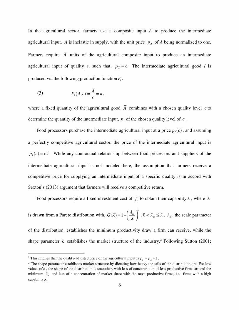
In the agricultural sector, farmers use a composite input A to produce the intermediate

agricultural input. A is inelastic in supply, with the unit price A

p of A being normalized to one.

Farmers require A units of the agricultural composite input to produce an intermediate

agricultural input of quality c, such that, A

p c= . The intermediate agricultural good I is

produced via the following production functionI

F :

(3) ( , )I

AF A c n

c= = ,

where a fixed quantity of the agricultural good A combines with a chosen quality level c to

determine the quantity of the intermediate input, n of the chosen quality level of c .

Food processors purchase the intermediate agricultural input at a price ( )I

p c , and assuming

a perfectly competitive agricultural sector, the price of the intermediate agricultural input is

( )I

p c c= .1 While any contractual relationship between food processors and suppliers of the

intermediate agricultural input is not modeled here, the assumption that farmers receive a

competitive price for supplying an intermediate input of a specific quality is in accord with

Sexton’s (2013) argument that farmers will receive a competitive return.

Food processors require a fixed investment cost of e

f to obtain their capability λ , where λ

is drawn from a Pareto distribution with, ( ) 1

k

mGλ

λλ

= −

, 0

mλ λ< ≤ .

mλ , the scale parameter

of the distribution, establishes the minimum productivity draw a firm can receive, while the

shape parameter k establishes the market structure of the industry.2 Following Sutton (2001;

1 This implies that the quality-adjusted price of the agricultural input is 1

I Ap p= = .

2 The shape parameter establishes market structure by dictating how heavy the tails of the distribution are. For low

values of k , the shape of the distribution is smoother, with less of concentration of less-productive firms around the

minimum m

λ and less of a concentration of market share with the most productive firms, i.e., firms with a high

capability λ .

7

2007), a firm’s capability can affect both final good quality and the costs of producing that final

good. In the literature, alternative interpretations of λ include skill, or the firm’s entrepreneurial

ability, but technically speaking, it is a heterogeneous measure used to sort firms into non-

exporter/exporter status. Additionally, in line with the Melitz (2003) class of models, every

participant in the final good market has an exogenous chance δ of exiting the market. If food

processors actively participate in their domestic market, there is a fixed cost of production f , and

if they are also capable enough to exporting, they incur a fixed cost of exportingX

f f> in all

periods. These, as well as the fixed costs of entry are in accord with Sexton’s (2013) observation

that food processing firms incur substantial investment costs. Note that since there is no cost to

product differentiation, it is possible to treat the capability parameter λ as an index of all firms

and all varieties of goods.

Production of the final good by food processors requires inputs of capability, the

intermediate agricultural input, and a composite input φ of a specific quality. The composite

input φ is most easily thought of in terms of the quality of a capital input which plausibly affects

the quality choice of the firm. For example, it might be equipment required to ensure quality

control in meeting food safety standards. The key point is that the composite input is a tangible

input required in production, since intermediate agricultural inputs by themselves are unlikely to

impact the final product-quality choice of the firm without being combined with some other

input(s) or transformed via another input. In effect, use of a composite input more accurately

reflects the technology choices available to and made by food processing firms. Importantly, φ

may vary across developed and developing countries, capturing the idea that the latter may have

8

a harder time meeting developed country food standards due to endowments of lower-quality

physical and/or human capital inputs.

The production function for the final good is given as:

(4)

( )

( )

( )

a

I

a

IX a

nF n

p cMC

p cMC

λ

φ

φ

λτφ

λ

=

=

=

In (4), the variables are defined as follows: n is the number of units of the intermediate

agricultural input used; 0a > represents a firm’s ability to translate capability into lowering

costs; MC is the marginal cost of producing the good for the domestic market, and X

MC is the

marginal cost of producing goods for export, where 1τ ≥ are the ad valorem costs of exporting –

including export taxes, import tariffs, the tariff-equivalent of non-tariff barriers and other

transport costs. As seen in (4), the production function is decreasing in the quality level of the

composite input, implying that the marginal cost of the firm is increasing in φ . Intuitively,

making a higher quality choice should come with an associated opportunity cost, e.g., a higher

quality machine capable of meeting higher food quality standards would have a higher rental rate

of capital than a lower quality machine. While there are many ways to model this stylized fact,

the simplest integration of φ into the model is adopted, whereby the cost of the composite input

is simply pφ φ= .

Food processors are also constrained by their quality choice. Expanding on the first variant

of Kugler and Verhoogen (2012), the firm’s quality choice reflects a complementarity between

their capability draw ( λ ), the quality of a composite input (φ ), and their intermediate

agricultural input quality choice ( c ), an approach that draws on the O-ring production function

9

concept of Kremer (1993). All three elements in the vector , ,λ cφ are complements in

producing quality, whereby quality is determined via a log-supermodular function, i.e., a food

processor with higher capability, using higher-quality intermediate agricultural and composite

inputs produces a higher-quality food product (Costinot 2009). Essentially this assumption rules

out capability being a substitute for low-quality agricultural and composite inputs. Of course,

there are other ways to formulate this quality constraint, but recent empirical evidence presented

by Brambilla, Lederman and Porto (2012) suggests that it is not an unreasonable assumption.

Food product quality q, therefore, is assumed to behave according to the following function,

(5) ( ) ( ) ( )1

3 31 1 1,

3 3 3

bq cββ β β

λ φ

= + +

where 0β < represents the degree of complementarity between the three determinants of final

good quality and 0b ≥ represents the scope of product-quality differentiation.3

This scope of differentiation parameter has traction in the literature as an approximation to

the fixed costs of investment required for product differentiation, i.e., it represents the ability of a

firm to differentiate product-quality in any capacity, through say R&D expenditures, advertising

and upgrading of productive inputs.4 In effect, this parameter acts as an additional channel

affecting firms’ quality choices. In particular, a lower value of b effectively restricts the quality

3 In general, the constraint relies on the following assumptions: ( ) ( ) ( )1 2 3

1b

q cβ β β βξ ξµ λ µ µ φ = + +

, where

1 2 20 1µ µ µ< + + < and 1ξ > is sufficient. The generalized multi-input quality condition can be written as:

( )1

1v

v vi

qβ β

µ χ=

= ⋅∑

, where ( )0,1v vµ ∈∑ , 0β < , and v

χ corresponds to each individual input used in the firm’s

production function, i.e. c , φ . Inputs that are not capability have the functional form: v

ξχ ϖ= , 1ξ > , and ϖ is

the additional input. When the input is the firm’s capability, the functional form isb

vχ λ= .

4 An alternative interpretation of b is the willingness of consumers to pay for quality.

10

choices available to a given firm, such that a firm with a higher b or a larger scope of

differentiation parameter will, ceteris paribus, have a higher quality choice available to them,

i.e., a quality choice closer to the world frontier of possible quality choices. As with φ , b may

also vary across developed and developing countries, the latter typically being farther from the

world quality frontier. This ability to translate capability into quality is an important component

of a firms’ quality choice that this analysis examines in detail.

Before continuing, it is important to justify the use of a third input, φ in both the production

function and the quality constraint. The food-processing industry purchases intermediate

agricultural inputs produced upstream in order to convert them into a final good. Using the

Kugler and Verhoogen (2012) two-input model in the food-processing context ignores the fact

that for this particular industry, a third input is typically required to convert the agricultural input

into the final good, since a firm’s “capability” or entrepreneurship does not accurately reflect the

processing required to generate a final good. This is particularly true in the context of quality-

differentiated final goods: a firm’s entrepreneurial capability is unlikely to be the sole

determinant of food quality outside of the quality of the agricultural input, especially since this

composite input might be necessary to ensure that a firm’s final good meets a particular food

quality standard. Additionally, accounting for a third input allows for further testing and pushing

of the Kremer (1993) O-ring assumption on the quality constraint that underpins this analysis:

i.e., all inputs must be complements in the firm’s quality choice, including the added composite

input. The inclusion of an additional input not only generates unique results in equilibrium, but is

easily translatable into an empirical setting for testing.

Overall, this modeling of quality choice dictates that more productive firms are more

capable of upgrading quality, and that this capacity to upgrade quality is contingent on matching

11

the productivity with higher quality intermediate agricultural and composite inputs. In this

context, firms optimize the following profit function:

(6)

( )

( ) ( ) ( )

,

1

3 3

( ) ( ), , , |

1 1 1 s.t. ,

3 3 3

I IO O O X Xa a

b

p c p cp c z p x f Z p x f

q cββ β β

φ τφπ φ λ

λ λ

λ φ

= − − + − −

= + +

where 0,1Z ∈ is an indicator of export status, 1Z = for firms that export and 0Z = being for

firms that produce only for the domestic market.

Equilibrium

As noted earlier, the intermediate agricultural input market is assumed to be perfectly

competitive in equilibrium, implying that for each and every quality choice in equilibrium, the

intermediate input price ( )I

p c c= . Therefore, optimizing equation (6) yields the following in

equilibrium:

(7a) * * 3( ) ( )b

Ic pλ λ λ= =

(7b) * 3( )

b

φ λ λ=

(7c) *( ) bq λ λ=

(7d)

2

* 3

2

* 3,

( )1

( )1

ba

o

ba

O X

p

p

σλ λ

σ

σλ τλ

σ

−

−

=

−

=

−

(7e) ( )1

* 1 1( ) 1r Z XP

σ

σ η σσλ τ λ

σ

−

− − = +

,

where * *( ) ( )I

c pλ λ= is the equilibrium intermediate agricultural input price and quality choice,

*( )φ λ is the equilibrium quality choice of the composite input, *( )q λ is the equilibrium output

12

quality choice by the firm, * ( )O

p λ is the domestic output price, *

, ( )O X

p λ is the export output

price, *( )r λ is the equilibrium revenue for the firm, and ( )1

3

baη σ

≡ − +

. (See Appendix for

equilibrium calculations).

3. Model Results

Impact of Scope

Equations (7a)-7(e) can be used to derive a set of key comparative statics, although for the

results to hold, 3

2

ab > must also be true. This condition essentially states that the scope for

quality differentiation b must be sufficiently large enough: in this case, b must be larger than

the firm’s cost-reduction capabilities for the following predictions to be true. At this point, it

should be noted that the equilibria described in equations (7a) through (7e) generate several

comparative static results. Two that are not addressed in detail here, but are relevant, are that the

agricultural input price and output price ( Ip , O

p and ,O Xp ) are increasing in b . This implies that

with an improved ability to translate capability into quality, firms end up charging a higher

output price (both for domestic and foreign markets), and pay a higher input price.

Output Quality and Firm Characteristics

Comparative statics that are derivable from the equilibrium yield the following results:

(8a) ( )

( )

*

21

1ln0

1

b Zq

Z

σ

σ

σ τ

τ η τ

−

−

−∂= <

∂ +,

(8b) *ln

ln 0q

bλ

∂= >

∂,

(8c) * * 3( ) ( )

b

c λ φ λ λ= = .

These results can be summarized as follows:

13

First, from (8a) the impact of trade costs (τ ) on the firm’s quality choice is shown. The

quality choice of the firm’s produced good ( r and q , respectively) increases with falling trade

costs. (8b) highlights the impact of firms’ ability to translate capability into quality ( b ) on the

firm’s quality choice (q). When a firm is better able to translate capability into quality, firms in

the market are able to produce higher-quality goods. Last, given (8c), firms treat all inputs as

complements and use correspondingly equal units of each. To produce the final good at a higher

quality level, then it must be true that firms use higher quality agricultural and composite inputs.

This result follows from the Kremer (1993) O-ring assumption: to produce a good with a higher

quality, firms require higher levels of all inputs used in the production process. Conversely, if a

higher quality final good is observed, then it must be true that firms are using complementary

levels of all relevant inputs, i.e., agricultural and composite inputs, and capability.

The first and second results focus on the impact of the exogenous variables τ and b on

quality choice, q . Falling trade costs and an increased ability to upgrade quality allow firms to

produce at a higher quality, and they increase in size as well based on revenue. This implies that

firms in the market increase market share and their quality choice when trade costs fall or when

b increases. Given that these firm characteristics are functions of λ , this implies that firms that

increase their size and quality choice as a result of these changing parameters increase their

productivity as well. This, combined with (8c), implies that firms that improve quality due to

falling trade costs or an improved ability to upgrade quality, do so by concurrently selecting

higher qualities of the agricultural input, c , the composite input, φ , and an increased λ .

A graphical representation of these theoretical results can be found in figure 1. Specifically,

the figure maps out the impact of trade costs and the ability of firms to translate capability into

quality on the quality choice of the firm. ( )1, 0q b Zλ = is the product quality relationship for the

14

domestic market, i.e., 0Z = , where 1b is ability to translate capability into quality. If firms

choose to export, though, they may face trade costs. Assuming that this ability to upgrade

quality, 1b , holds, then firms that wish to export cannot choose the same quality and must choose

a lower input and output quality for a given λ since trade costs not only impact the quantity

produced, but the quality level as well, as shown through by ( )1, 1q b Zλ = ). Of course, if trade

costs fall, this pushes ( )1, 1q b Zλ = up towards ( )1, 0q b Zλ = , thereby raising export-quality for

any value of λ equal to or above the export entry cutoff point*

X bλ . In other words, lowering

trade costs has the potential to raise export quality.

However, firms’ quality decisions may change based on their ability to upgrade quality. If 1b

increases to 2b , firms’ optimal choices may change. If the increase to 2b is sufficient to outweigh

trade costs τ , then it will be possible for exporting firms to select a higher quality due to this

improved ability to translate their capability λ into quality q outweighing the costs associated

with exporting the good to that destination, given by ( )2 , 1q b Zλ = . In other words, it may not

be so surprising that an increased ability to translate capability into quality can result in increased

exports of high-quality food products. However, as will be shown subsequently, the domestic

market entry threshold and the export market entry threshold are both affected by changes in

ability to translate capability into quality .b Therefore, the impact of b increasing is considered

here in a situation where the equilibrium thresholds * bλ and *

X bλ are fixed.

Figure 1 also highlights the fact that some firms might still export despite high trade costs.

For trade costs ofτ ′ , it is possible for production and export at a given level of quality choice q′

and a given ability to translate capability into quality 1b . At first glance, if trade costs are too

15

high, we would expect firms to choose not to export and instead produce only for the domestic

market. However, for a given quality level, it is possible for some firms to still produce at that

quality and export. For a firm to still produce at a given quality level in the face of stiff trade

costs, it would necessarily imply that the firm’s capability or productivity bλ′ would have to be

sufficiently greater than the export cutoff of *

X bλ to maintain production at quality level q′ . This

behavior would be especially true if values of b across countries were low enough to not be

conducive to trade.

Importantly, these results are empirically testable: the model clearly indicates that with

regards to the firm’s quality choice, falling trade costs and an increased ability to upgrade quality

will allow firms to choose to produce higher-quality goods. In addition, this affects the input

quality choices that firms make: larger firms, who choose to produce higher quality final goods,

should select higher qualities of both the composite input and the agricultural input.

Impact of Trade Liberalization and Changes in Ability to Upgrade Quality

As shown in the previous section, it is possible for firms to select into producing higher quality

when their ability to translate capability into quality increases. Establishing when firms make

this switch is critical.5 By utilizing the following equilibrium conditions:

(9a)

* ** ( )

( ) 0dd

rf

λπ λ

σ= − = and,

(9b)

* ** ( )

( ) 0x xx x

rf

λπ λ

σ= − = ,

5 To solve for this equilibrium, assume that the Pareto distribution’s shape parameter max( ,1)k η= is true, such that

the means of the revenues will be finite.

16

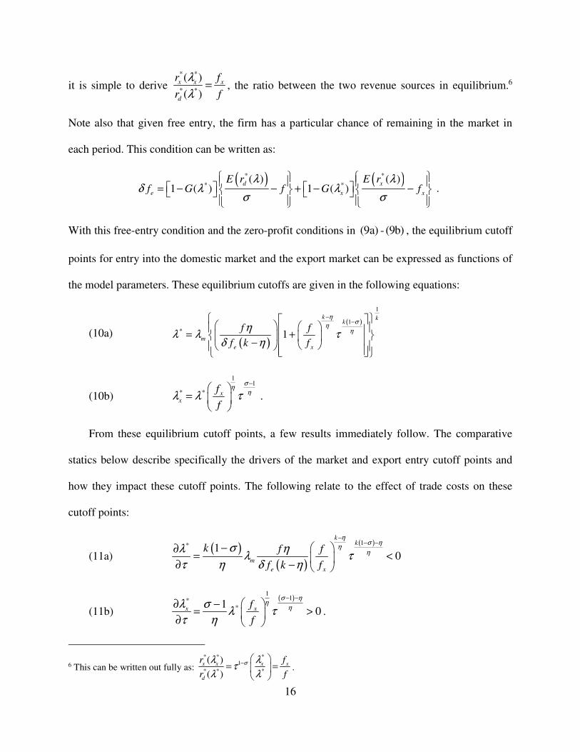
it is simple to derive

* *

* *

( )

( )

x x x

d

r f

r f

λ

λ= , the ratio between the two revenue sources in equilibrium.6

Note also that given free entry, the firm has a particular chance of remaining in the market in

each period. This condition can be written as:

( ) ( )* *

* *( ) ( )

1 ( ) 1 ( )d x

e x x

E r E rf G f G f

λ λδ λ λ

σ σ

= − − + − −

.

With this free-entry condition and the zero-profit conditions in (9a) - (9b) , the equilibrium cutoff

points for entry into the domestic market and the export market can be expressed as functions of

the model parameters. These equilibrium cutoffs are given in the following equations:

(10a) ( )

( )

1

1

* 1

k kk

m

e x

f f

f k f

ησ

ηηη

λ λ τδ η

−−

= + −

(10b)

11

* * xx

f

f

ση

ηλ λ τ−

=

.

From these equilibrium cutoff points, a few results immediately follow. The comparative

statics below describe specifically the drivers of the market and export entry cutoff points and

how they impact these cutoff points. The following relate to the effect of trade costs on these

cutoff points:

(11a) ( )

( )

( )1* 10

kk

m

e x

k f f

f k f

ησ η

ηησλ η

λ ττ η δ η

−− −

− ∂= <

∂ −

(11b)

( )1

1**1

0x xf

f

σ ηη

ηλ σλ τ

τ η

− − ∂ −

= > ∂ .

6 This can be written out fully as:

* * *1

* * *

( )

( )

x x x x

d

r f

r f

σλ λτ

λ λ−

= =

.

17

The results described in (11a) and (11b) can be summarized as follows: from (11a), given

that *

0λ

τ

∂<

∂, falling trade costs increase the equilibrium domestic market entry cutoff point

*λ ,

implying that the least productive firms will be shut out of the market and be forced out of

production with falling trade costs. In addition, (11b) shows that *

0λ

τ

∂>

∂, such that falling trade

costs lower the equilibrium export entry cutoff point *

xλ , implying that more firms will choose to

enter the export market given falling trade costs. Those firms that are now able to export were

previously the most productive non-exporters in the market, but given falling trade costs, they

can now enter the export market.

These results are intuitive, conforming to the existing literature on heterogeneous firms and

trade. When trade costs decrease, more firms should be able to enter the export market, since the

barriers to trade that previously hindered a given firm from entering the export market are being

reduced or eliminated altogether. However, this entry into the export market by more firms

redistributes the overall revenues of the sector: firms entering the export market increase their

revenue, but in doing so push out the smaller and less capable firms from the market, altering the

structure of the market. Therefore, the classic heterogeneous-firms and trade conclusion is

supported here: falling trade costs induce entry into the export market by the most capable non-

exporters yet cause the least capable firms in the entire market to exit altogether since they are

unable to compete with the larger firms. This has obvious implications in the context of

Sexton’s (2013) observations concerning contracts with agricultural input suppliers: with trade

liberalization, some will either not be offered contracts by food processors or will at least receive

lower prices if they produce lower-quality inputs, while other suppliers get higher prices for

18

producing higher-quality inputs as some food processing firms either enter the export market of

expand their export market share.

Another channel that impacts the equilibrium cutoff points is the ability of firms to

transform capability (λ ) into quality, b . The following comparative statics are informative:

(12a)

( ) ( ) 3

*

32

ln 1 ln

3

k kk

a b

k

X X Xba

m

e

f f f

f f ff

kb f

η

η η

σ τ ρ τ

λ λτ

δ ρ

−−

+−

+

− − Λ − + ∂ =

∂ Λ

(12b) ( ) ( )

11*

*

2

1ln 1 ln

3

x

X X

f f

b f f

ση

ηλ σλ τ σ τ

η

− ∂ − = − + − ∂

.

Note that ( )3 kηΛ = − and ( )3X

fa b

fρ

= +

. The signs on both (12a) and (12b) are both

ambiguous, since they depend on varying factors. The sign on (12a) is dependent on the

following condition:

(13a) *

0b

λ∂<

∂ when k η γ< + , and vice versa.7

The above expression, k η γ< + , implies that when η is sufficiently large, i.e., the sum of

firms’ ability to reduce costs via capability ( a ) and their ability to translate capability into

improving quality ( b ), and k is sufficiently small, then an increased ability to convert capability

into higher quality allows more firms to enter the domestic market since the cutoff point

decreases, *

0b

λ∂<

∂. Here, an improved level of “quality upgrading” is enough to allow firms to

7 For convenience, ( ) ( )31 ln 1 ln 01

kk

a b

X X

f f

f f

η

ηηγ τ σ τ

σ

−−

+

= − + − − > −

.

19

enter the domestic market, given a sufficiently low k . Since firms are distributed along a Pareto

distribution with shape parameter k , a sufficiently low k implies that the distribution of firms is

“smooth” enough, in that firms are not too “clumped up” near m

λ , implying that for a given λ ,

the number of close competitors with a sufficiently close λ capability draw is relatively low, and

that the market is not dominated by just a few firms. Thus, for increases in b , this spread-out

distribution of firms in the market implies that there is sufficient “room” in the market for new

firms to come in and take a share of the domestic market, since the more productive firms do not

occupy a sufficiently large enough share of the market to keep out potential entrants with an

increasing ability to translate capability into quality.

When k η γ> + , then c, such that the domestic market entry cutoff point rises with an

increasing ability to translate capability into quality. This is due to the fact that with a

sufficiently high k , the distribution of firms along λ is characterized by many firms “clumped

up” towardsm

λ . Intuitively, this implies that many firms make up the bottom of the distribution

while firms at the top end of the distribution control a large market share. Combining these two

facts, the model shows that the firms at the top end of the distribution are able to expand their

market share when b increases, and that there are too many firms at the bottom of the

distribution. With firms at the top occupying a larger market share and a fat left tail of the

distribution, a bottleneck effect is generated wherein an increased ability to upgrade quality

actually prevents firms from entering the domestic market, since there is not sufficient room in

the market for the number of firms to enter with the most productive firms increasing their

market share and pushing out the least productive firms in the process.

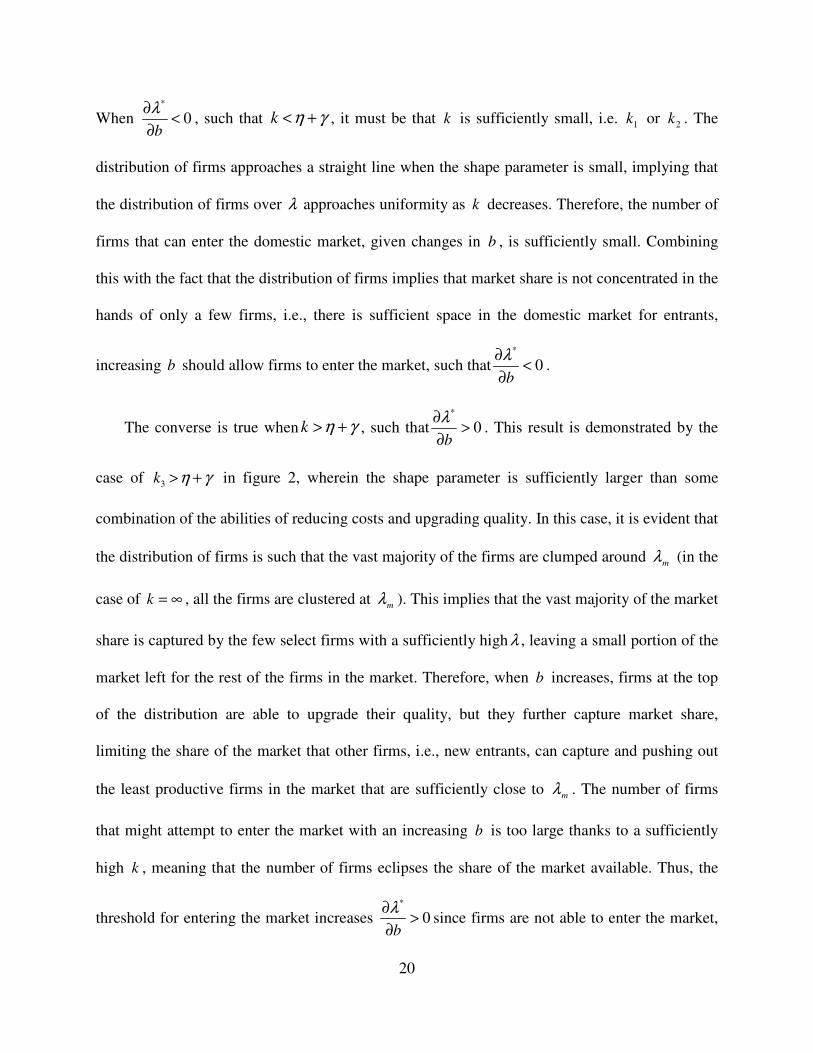
These results can be more clearly seen by referring to figure 2, a graph of the cumulative

distribution function of the Pareto distribution with a minimum m

λ and a shape parameter k .

20

When *

0b

λ∂<

∂, such that k η γ< + , it must be that k is sufficiently small, i.e. 1k or 2k . The

distribution of firms approaches a straight line when the shape parameter is small, implying that

the distribution of firms over λ approaches uniformity as k decreases. Therefore, the number of

firms that can enter the domestic market, given changes in b , is sufficiently small. Combining

this with the fact that the distribution of firms implies that market share is not concentrated in the

hands of only a few firms, i.e., there is sufficient space in the domestic market for entrants,

increasing b should allow firms to enter the market, such that*

0b

λ∂<

∂.

The converse is true when k η γ> + , such that*

0b

λ∂>

∂. This result is demonstrated by the

case of 3k η γ> + in figure 2, wherein the shape parameter is sufficiently larger than some

combination of the abilities of reducing costs and upgrading quality. In this case, it is evident that

the distribution of firms is such that the vast majority of the firms are clumped around m

λ (in the

case of k = ∞ , all the firms are clustered at m

λ ). This implies that the vast majority of the market

share is captured by the few select firms with a sufficiently highλ , leaving a small portion of the

market left for the rest of the firms in the market. Therefore, when b increases, firms at the top

of the distribution are able to upgrade their quality, but they further capture market share,

limiting the share of the market that other firms, i.e., new entrants, can capture and pushing out

the least productive firms in the market that are sufficiently close to m

λ . The number of firms

that might attempt to enter the market with an increasing b is too large thanks to a sufficiently

high k , meaning that the number of firms eclipses the share of the market available. Thus, the

threshold for entering the market increases *

0b

λ∂>

∂since firms are not able to enter the market,

21

and the least productive firms are forced to exit since the space remaining in the market for the

least productive firms decreases as firms at the “top” end of the distribution, i.e., high λ , further

increase their market share.

Returning to (12b), the sign on *

x

b

λ∂

∂is also ambiguous. The result hinges on the sign of the

following expression:

(13b) *

0x

b

λ∂<

∂ when, ( ) ( )ln 1 ln 0

X

f

fσ τ

+ − >

, and vice versa.

Immediately, ( )ln 0X

ff

< since X

f f< , and so for an increased ability to translate

capability into higher quality to result in a lower equilibrium export market entry cutoff point,

depends on two things: the extent that X

f f> , and the additional rents incurred from exporting,

given that there is a price markup when exporting. With X

f f→ , such that the fixed costs of

exporting are not “drastically” higher than the fixed costs of entering the market, then *

0x

b

λ∂<

∂

with sufficiently high export price markup ( ( ) ( )1 lnσ τ− ). This implies that firms’ improved

ability to translate capability into quality is able to overcome the fixed costs of exporting,

meaning that firms are now able to enter the export market, given that the additional rents from

entering the export market outweigh the costs of doing so. However, if X

f f<< , then an

increased ability to upgrade quality actually yields *

0x

b

λ∂>

∂, such that firms will exit the export

market. This is due to two facts: the first that the fixed costs of entering the export market are

much higher, implying that an increasing ability to upgrade quality is not sufficiently “strong”

enough to overcome those fixed costs, but also due to the fact that the fixed costs of exporting

22

sufficiently outweigh any rents earned due to exporting. Thus, firms who previously found it

worthwhile to export will now exit the export market with the increase in the ability to translate

capability into quality (since X

f must be paid in each period).

As with the results from equation (8), the results contained in equations (11) and (12) are

also empirically testable. Unequivocally, falling trade costs should cause the most productive

non-exporters to enter the export market, while the least productive firms in the market are

forced to exit altogether. While the effects of the ability to translate capability into quality on

these equilibrium threshold are ambiguous, the empirical tests will prove to be telling about the

other model parameters, such as the shape of the Pareto distribution ( k ), the level of cost-

reduction and quality upgrading in a firm (η ), or even the level of fixed costs that a firm must

pay to export in a given period (X

f ).

Before considering empirical application of the model, the above comparative statics require

an increase in b across the board as it is not firm-specific. Importantly, the results highlight the

importance of market structure in determining the impact of changing the ability to translate

capability into quality, and conversely how those changes in b also alter market structure. First,

from (12a), the comparative statics are heavily dependent on the Pareto distribution’s shape

parameter k . Recall that the shape parameter determines the distribution of firms along λ . If k is

high, then firms are more concentrated at the bottom end of the distribution and there are a few

select firms at the top of the distribution, with high values of λ . These few firms at the top of the

distribution hold a larger share of the market than the firms at the bottom of the market, implying

that the market is structured to favor those fewer, more productive firms over the more numerous

firms at the lower end of the distribution. Therefore, the comparative statics suggest that *

0b

λ∂>

∂

23

when b increases, where the structure of the market becomes further skewed in favor of those

firms with a high λ . Those firms are able to capitalize on an increasing b to consolidate their

market share, which not only restricts entry by potential entrants (who are closer to the bottom of

the distribution), but also pushes out the least productive firms in the market.

If k is low, then the opposite effect occurs, since the distribution of firms over λ is

smoother and more even. Firms are dispersed more evenly over the distribution, implying that

the market share is more “equally” allocated between firms in the market and that the market is

structured such that many firms can enter and compete. Thus when b increases, the comparative

statics show that *

0b

λ∂<

∂. Since no firm(s) have a dominant market share, the market is more

open to competition, so an increase in b allows new firms to enter the market, thus further

spreading out the market share among both new entrants and firms already in the market.

Likewise, the results from (12b) relate specifically to the market structure of exporters. The

sign on *

x

b

λ∂

∂ is contingent on the size of the parameter

Xf , especially the degree to which

Xf f>

. Since X

f f> by assumption, this implies already that the most productive firms in the market

can overcome X

f to become exporters. Higher values of X

f mean that there are fewer firms in

the market export, but those that do export, have a sufficiently high λ and capture export market

share. Thus, from (12b), if Xf f→ such that X

f is not too large, then an increase in b means

that since Xf is small enough, that this improved ability to translate capability into quality

allows the most productive non-exporters entry into the export market since their added revenues

from exporting now outweigh the fixed costs of exporting. Thus, with *

0x

b

λ∂<

∂, the export

market gains new entrants, making the export market more competitive than previously.

24

However, if Xf f>> , then

*

0x

b

λ∂>

∂. An increased ability to translate capability into quality

favors the most capable firms. These firms are able to upgrade their quality and gain more of the

export destination market share. The least productive exporters are actually forced out of the

export market because the revenues from exporting are now no longer sufficiently high enough

to outweigh the fixed costs of exporting with the most productive firms taking a now-larger share

of the market. Thus, with the least productive exporters exiting the export market, the market

structure changes such that it becomes less competitive, with fewer, more productive and larger

firms taking the entirety of the market share.

4. Empirical Analysis

Data

The data used in the empirical analysis come from Chile’s Encuesta Nacional Industrial Annual

(ENIA), which tracks all firms in Chile in a robust, unbalanced panel data set for the period

2001-2007. This data set, maintained by Chile’s Instituto Nacional de Estadísticas, tracks a

multitude of firm-level characteristics, input choices, in addition to many value-added measures

that form the basis of the quality variables used in the analysis. The focus of the analysis in this

paper concerns the food-processing industry, which yields a sample size of 11,196 observations

over the seven-year sample, with a fairly even distribution of approximately 1,600 firms per year

in the sample.

In particular, the data set is used to calculate aggregate estimates of output quality and

various input quality choices. Unlike the Colombian data set used by Kugler and Verhoogen

(2012), Chile’s ENIA does not track unit values of either output or inputs. Therefore, the

measures used in the empirical analysis are designed to approximate the overall quality choices

made by the firm, in terms of both output and inputs. This is achieved by relying on the wealth of

25

value added variables contained in the ENIA dataset. Of course, only using the raw values for the

value added of production does not properly account for the size of the firm’s production.

Therefore, each measure divides the variable by the total value of either production or the cost of

goods to calculate the share of value added. For example, a firm’s quality choice ( q ) is

approximated by value added as a share of their revenues (i.e., the value of production). In

addition, intermediate agricultural input quality ( c ) is given by the value added cost of raw

materials as a share of the total cost of goods.

The measure for φ utilizes the fact that this input is treated as a composite input. While it

typically can be considered as capital required to ensure that a particular level of food quality is

met, it can also represent other inputs that might ensure food quality, such as land or other

facilities. Therefore, φ is measured as the current value of land, buildings, and machinery

(including those in progress) combined with the cost of refrigeration and storage as a share of the

total cost of goods. The cost of refrigeration and storage here is unique to the food industry case,

since obviously the storage of food is necessary to ensure that the any final food-industry

products remain at the same quality level produced, i.e., that they do not spoil before arriving at

their destination. Given that the variable b relates specifically to the idea of a firms’ ability to

translate capability into quality, the variable focuses on new expenditures by firms that might

impact quality, i.e., new land, buildings, and machinery. Thus, b is defined as the sum of the

purchase of new inputs that may impact quality as a share of the total cost of goods. While these

formulations are admittedly similar, φ importantly reflects the current value of the composite

input while b captures new expenditures that might affect quality, so the two parameters capture

different effects.

26

The construction of the rest of the variables largely follows the broader literature. Freight

costs in the following analysis are given at the firm level instead of the typical industry level,

providing an additional level of detail not found in other studies, such as in Kugler and

Verhoogen (2012). Ad valorem freight rates are calculated here as the value of export costs to

ship the good to the destination as a percentage of the value of export revenues8. Tariff rates are

imported into the data at the industry level using the TRAINS database provided by the World

Integrated Trade Solution (WITS). Lastly, the productivity parameter (λ ) is an adjusted labor

TFP measure, where λ is the firm’s TFP divided by the average TFP in that firm’s industry.

Summary statistics for the relevant variables can be found in table 1.

A few things that stand out from the summary statistics are worth noting before proceeding

with the empirical analysis. First, the share of firms that export in this sample is low. Only 4.2%

percent of firms chose to export over the period 2001-2007. Through the theoretical model, this

might suggest that most of the firms do not have the required capability, i.e., productivity, to

export. Examining the cumulative distribution of the productivity parameter (λ ) shows that this

is likely the case. Figure 3 shows that 90% of the firms in this sample have a productivity of less

than 35.33, and 99% of the firms in the sample have a productivity of less than 118.67. Based on

this distribution, it is apparent that there are many low-productive firms and only a few very-

productive firms who capture the vast majority of the market share.

Given that the percentage share of exports in total sales revenue has a mean of 11.44 percent

across firms, this suggests that firms that have the capability to export, do not actually export that

much. Next, q has an average value of 0.388, indicating that value added by firms is 38.8

8 This usage differs slightly from the literature, but is based on the theoretical construction. As given in equation (6),

trade costs only impact export revenues, not total revenues.

27

percent of the total value of production, a sizable amount. This implies that food-processing

firms choose to produce final goods at quality levels requiring considerable value added.

Last, consider the levels of b , c , and φ . These values are all quite low, suggesting that

firms do not spend a significantly large portion of their costs on either the agricultural input, the

composite input, or investments that improve their ability to translate capability into quality,

although, the value-added expenditures on agricultural inputs has the largest share of costs, at 11

percent. However, given that the measure of q suggests that firms add a considerable amount of

value to the final good, it is possible that firms are rather easily able to translate the quality both

of those agricultural inputs and their ability to upgrade quality into a realized level of quality.

Empirical Specifications

The empirical work described here loosely follows the structure of Bernard, Jensen, and Schott

(2006). Separate regressions test the comparative statics derived in the theoretical analysis. First,

the impact of model parameters, i.e., b , c , φ , τ on a firm’s chance of entering the export market

is tested. The second specification tests the impact of the parameters on a firm’s chance of

exiting the market altogether. Third, the impact of the model parameters on the firm’s quality

choice is tested. To briefly summarize, falling trade costs should increase the chance of firms

entering the export market and cause the least productive firms to exit the market, and improve

the firms’ quality choices. An increase in the ability of firms to upgrade quality has an

ambiguous impact on the chances of firms exiting the domestic market and entering the export

market (due to other parameters), and improves the firms’ quality choice. In each of these

specifications, a test for the complementarity of the inputs is implemented as well. The model

anticipates that higher levels of all three inputs ( c , φ , λ ) would be associated with a higher

probability of entering the export market, a lower probability of exiting the market, and a higher

28

quality choice. A list of the expected signs of the key parameters is given in table 2, while the

full set of empirical results is reported in table 3.

A. Quality Choice

To test how the model parameters impact the firm’s quality choice, a reduced-form fixed-

effects approach is utilized. In particular, the specification controls for industry fixed-effects in

its analysis of quality choices:

(14) ( )1 2 j tq c b b Xα β β φ γ δ τ µλ κ ξ ψ ε= + + + + ∆ + + Γ ⋅ Ψ + + + + .

This specification simply uses the chosen quality level, q , as the dependent variable as

opposed to changes in quality levels. This formulation of the dependent variable is used

specifically because the model states that firms make their quality choices in each period. c and

φ are the quality levels of both the agricultural input and the composite input respectively, τ∆

is the change in trade costs, λ is firms’ capability, represented by firms’ total factor productivity,

b ⋅Ψ represents the interactions between b and the vector of inputs , ,c φ λ , and X is a vector

of firm characteristics. Results for this specification are shown in column [1] of table 3.

In general, the signs on the point estimates align with the theory. Though insignificant, there

is some limited evidence for the idea that falling trade costs should increase firms’ quality

choice, as given by equation (8a), though this empirical evidence is inconclusive. This partial

evidence is not necessarily surprising, however, given figure 1. Firms who have *

Xλ λ< and are

sufficiently far enough away will not have their quality choices impacted by falling trade costs

since those firms are too far away from the export entry cutoff point, which is plausible given the

skewed distribution of productivity in food-processing industries (see figure 3).

The empirical specification generally shows statistically significant support for the quality

constraint used in the theoretical model. First, the coefficient on φ is statistically significant and

29

positive, implying that firms with higher quality composite inputs produce at a higher quality

level. The coefficient for c is statistically significant and is negative, which does not support the

theoretical model. However, given the formulation of c as a percentage of total cost, it is

plausible that firms who spend more on higher quality inputs at the expense of other quality

inputs actually do produce at a lower quality level, thus generating this anomalous result. This

does imply that increasing the quality of the material input without increasing the quality of other

inputs (or the ability to upgrade quality) is not possible for firms who wish to upgrade their final

good quality, thus providing some evidence for the quality constraint. The impact of productivity

( λ ) on quality, while having the correct sign, is economically and statistically insignificant.

However, the interaction terms provide strong support for the quality constraint. All three

coefficients (for c b⋅ , bφ ⋅ , and bλ ⋅ ) are statistically significant at the 5% or better, and are

positive. This implies that for higher values of b , values of c , φ , and λ will be higher, and vice

versa. Therefore, the results predict that all three of these inputs (alongside b ) move in the same

direction, supporting the usage of the Kremer (1993) O-ring theory as the quality constraint. It is

also worth noting that given the larger positive coefficient on c b⋅ means that for firms with a

sufficiently large b , the overall impact of increasing c on q can, in fact, be positive. As the

theoretical model shows, the role of quality upgrading in a firm’s quality choices is very

important, as larger values of b allow firms to upgrade quality beyond merely improving the

quality of the agricultural input, the composite input, or productivity.

B. Export Entry

To test the impact of the model parameters on the chance that a firm enters the export market, the

approach popularized by Roberts and Tybout (1997) is used. This particular approach relies on

the observation that firms who export must overcome the fixed costs associated with entering the

30

export model ( Xf ). Therefore, this export condition is formulated into a probit specification that

tests how trade costs, the ability to upgrade quality, the agricultural input quality, and the

composite input quality all affect the chance of a firm entering the export market, given that the

firm was not exporting in the prior period:

(15) , 1 , 1 2Pr( 1 0)i t i tExport Export c b Xα β β φ γ δ τ µλ κ ε+ = = = + + + + ∆ + + +

, 1 ,Pr( 1 0)i t i tExport Export+ = = is the probability that the firm enters the export market in

time t given that the firm was not exporting in the prior period, c and φ are the quality levels of

both the agricultural input and the composite input, respectively, τ∆ is the change in trade costs,

λ is firms’ capability, represented by firms’ total factor productivity, and X is a vector of firm

characteristics.

The results from a probit specification can be found in column [2] of table 3. Importantly,

the model generates correct signs on most of the important parameters, typically with statistical

significance. First, both tariff and freight rates show that when they fall, firms are more likely to

enter the export market, providing strong evidence for the theoretical model, though no

significance on the interactions between λ and trade costs are found. A one-standard deviation

decrease in trade costs is associated with an economically significant 109.4% increased chance

of entering the export market, an extremely large effect9. This implies that firms are particularly

responsive to trade costs as well.

As given by the theoretical model, the impact of b , the ability to translate capability into

quality is ambiguous and depends on other model parameters. The sign on the coefficient

depends on the extent that Xf f> , and the additional rents earned by the firm when exporting,

9 Note that the standard deviation of the changes in freight rates ( 18.362

Freightσ ∆ = ) and tariff rates ( 1.07

Tariffσ∆ = )

are high, causing the magnitude of the impact to be that high.

31

given that there is a price markup when exporting. If the coefficient estimate is positive, it

implies improved ability to translate capability into quality (a higher b ) improves a firms’

chances of entering the export market, which implies that the fixed costs of exporting are not too

high relative to the fixed costs of entering the market, and that the rents earned from exporting

outweigh this additional fixed cost. This case is indicated by the results. The point estimate is

0.178γ = , and is significant at the 5 percent level, implying that a firms’ increased ability to

upgrade quality improves their chances of entering the export market. However, a one standard-

deviation increase in firms’ ability to upgrade quality only increases the chance of firms entering

the market by 2.64 percent, which is not a large effect, though it has some economic

significance.

The empirical specification also allows for a test of the validity of the quality constraint. The

equilibrium dictates that firms using higher quality inputs in all respects ( c ,φ , λ ) are more

likely to export. Therefore, the point estimates of the coefficients should all have a positive sign.

While all three estimates have the correct sign, the estimate forφ , 2β , is not statistically

significant, showing that the theory is generally supported by the results, though not completely.

11.305β = , the estimate for c , is statistically significant at the 1% level, implying that firms

with a higher level of agricultural input quality have a higher chance of entering the export

market. A firm with an agricultural input quality level one standard-deviation above the mean

has a 4.72 percent increased probability of entering the export market, which has some economic

significance. The coefficient estimate for λ , 0.016µ = , means that more productive firms are

more likely to enter the export market, in accordance with the theory. Increasing a firm’s

productivity level by one-standard deviation above the mean increases the chance that the firm

enters the export market by 4.88 percent, an economically significant amount. These effects

32

indicate an overall increased ability to enter the export market, where firms that are able to

upgrade the quality of their agricultural inputs and boost their productivity are more likely to

enter the export market.

C. Market Exit

The approach used above, wherein the Roberts and Tybout (1997) method tests for export entry,

is adapted to test for market exit of firms. Therefore, the approach relies on the observation that

firms who exit the market from one period to the next are no longer capable of paying the fixed

costs of production ( f ) required to remain in the market. Therefore, this market exit condition is

formulated into a probit specification that tests how trade costs, the ability to upgrade quality, the

agricultural input quality, and the composite input quality all affect the chance of a firm exiting

the market altogether given that, in the period before they were in the market:

(16) ( )

( ), 1 , 1 2Pr( 1 0)

i t i tExit Exit c b

b X

α β β φ γ δ τ µλ τ λ

κ ε

+ = = = + + + + ∆ + + Θ ∆ ⋅

+ Γ ⋅ Ψ + +

, , 1Pr( 1 0)i t i tExit Exit −= = is the probability that the firm exits the market in time 1t +

given that the firm was operating in the market in time t , c and φ are the quality levels of both

the agricultural input and the composite input, respectively, τ∆ is the change in trade costs, λ is

firms’ capability, represented by firms’ total factor productivity, τ λ∆ ⋅ introduces the

interactions between trade costs and productivity, b ⋅Ψ introduces the interactions between b

and the vector of inputs , ,c φ λ , and X is a vector of firm characteristics. The results from this

probit specification are shown in column [3] of table 3, and provide some support for the

theoretical model.

First, the impact of falling trade costs on market exit is mixed. The impact of changes in

trade costs are ultimately inconclusive, with the estimates typically being statistically

33

insignificant. The only statistically significant estimate is the interaction between freight rates

and λ , and its sign is negative, which does not appear to agree with the model. When trade costs

fall, the model predicts that less-productive firms should be more likely to exit the market, not

more-productive firms. However, as noted by Ai & Norton (2003) and used in Melitz-model

empirical studies such as Blyde & Iberti (2012), using the coefficient Θ to interpret marginal

effects yields incorrect inferences about the impact of falling trade costs, since Θ is calculated at

the average change in freight rates and productivity, leading to the average marginal effect.

Adjusting for these effects by calculating the marginal impact of changes in freight rates at

individual points shows that given falling trade costs (i.e., 0Freight∆ < ), then more productive

firms with a higher λ are less likely to exit the market than less productive firms, who are now

more likely to exit the export market. This correction essentially shows a positive estimation of

the interaction term, where the correction is statistically significant at the 10% level or better for

larger drops in freight rates.

The impact of increasing the ability to upgrade quality shows some unique results. The

coefficient estimate itself is positive and statistically significant at the 1% level, implying that

*

0b

λ∂>

∂, such that k η γ> + . This result has two ramifications: first, it states that on the whole,

the impact of cost-reduction for firms is fairly low and cannot overcome the fixed costs of

entering the market, and second, that the distribution of firms is skewed towards there being

many small firms in the market and a few much larger firms (such that the large firms capture an

increasingly large share of the market).

Additionally, this result is reinforced given the coefficients on the interaction terms,

especially the coefficient on c b⋅ , which is one of two statistically significant estimates at the 5%

level or higher. This coefficient states that for higher values of c , the impact of increasing a

34

firm’s ability to upgrade quality has a large negative effect on the chance that a firm exits the

market. Given the nature of the quality constraint used in the theoretical analysis, the model

predicts that firms with higher levels of c require higher levels of b (ceteris paribus), which

places firms farther away from the market exit threshold and vice versa. A similar relationship

exists given the negative coefficient on the interaction between λ and b , which shows the

importance of upgrading quality for a firm. More productive firms are more able to upgrade

quality, thus decreasing their chances of exiting the export market, and the reverse is true.

Therefore, there is some support for the quality constraint used in the model. The test for the

remaining elements of the quality constraint in this model do not currently provide any

discernible support for or against the model, at the 10% level of significance or better.

35

5. Summary and Conclusions

In this paper the heterogeneous firms and trade literature is extended by integrating quality of

inputs and outputs in a food and agricultural setting, along with an analysis of how the ability to

translate capability into higher product quality is critical in evaluating the cut-offs for food

processing firms to enter domestic and export markets.

In the theoretical analysis, it is found that the direction of change in the domestic market cut-

off point, due to an increased ability to raise quality, is quite sensitive to key parameters of the

capability distribution. Specifically, for a Pareto distribution, if the capability draw of firms is

fairly evenly distributed, raising the ability of firms to translate their capability into higher

quality allows more firms to enter the domestic market; by contrast, if the distribution of firm

capabilities has a fat lower tail, firms with higher capability expand their market shares at the

expense of lower capability firms. In the case of the export market cut-off, the direction of

change depends on the fixed costs of entry into and the rents available from exporting.

Specifically, if the fixed costs of exporting are quite close to the fixed costs of entering the

domestic market, with sufficiently high export price markups, firms are able to enter the export

market due to an increased ability to translate their capability into higher quality. The opposite is

true if the fixed costs of exporting are much higher than the costs of entering the domestic

market.

These and other hypotheses are then tested for using a panel data set for Chilean food

processors over the period 2001-2007. Based on these data, there is generally strong support for

the theoretical analysis. Empirical results concerning the export entry threshold *λ are strongly

supported by the model, wherein falling trade costs significantly promote export entry, and

quality upgrading sufficiently allows firms to overcome Xf to enter the export market while

36

providing fairly strong support for the quality constraint. The specification testing market exit

provides less strong support for the theoretical model, showing that falling tariff costs allow

firms to remain in the market (but also that less-productive firms are more likely to exit), and that

quality upgrading can help firms avoid firm exit for sufficiently high levels of input qualities and

quality upgrading. Close to the threshold *λ , however, market exit occurs more often as the

capability of cost-reduction of those firms cannot cover the fixed costs of entering the market.

This also implies that the distribution of firms along λ is fairly unequal, in that there are many

low-productivity firms and only a few high-productivity firms, with few in between, which is

actually seen in the data (i.e., figure 3).

The quality constraint has some fairly strong support from the empirical results, in that while

one of the estimates for the inputs ( c ) is negatively correlated with, results show that firms with

a higher ability to upgrade quality can use this to increase the quality of the inputs c , φ , and λ ,

further improving their ability to increase the quality of the final good (and vice versa, where

higher levels of c , φ , and λ imply that firms can also use these to improve the quality of their

final good by investing in the ability to upgrade quality, b )10. The negative coefficient for c can

actually be interpreted to support the theory, since the coefficient should be interpreted as ceteris

paribus, where solely increasing the quality of the material input (implicitly at the expense of

other inputs) corresponds to lower quality, implying that firms need to increase the quality of

these inputs at the same time as other inputs to attain higher levels of product quality.

10 This fact also lends credence to the conclusions regarding the structure of the food-processing industries in Chile.

Firms with high levels of all inputs are going to be choosing high quality levels of the final good, and thus will be

the very productive and largest firms in the market, while firms who lag behind in one input or the ability to upgrade

quality are going to be the smaller, less productive firms in the market.

37

Appendix

A sketch of how to derive the equilibrium results is as follows. Recall that:

(7a) * * 3( ) ( )b

Ic pλ λ λ= =

(7b) * 3( )

b

φ λ λ=

(7c) *( ) bq λ λ=

(7d)

2

* 3

2

* 3,

( )1

( )1

ba

o

ba

O X

p

p

σλ λ

σ

σλ τλ

σ

−

−

=

−

=

−

(7e) ( )1

* 1 1( ) 1r Z XP

σ

σ η σσλ τ λ

σ

−

− − = +

, ( )1

3

baη σ

≡ − +

.

First, with a perfectly competitive intermediate agricultural input market, * *( ) ( )I

c pλ λ= .

Writing the demand function x as a function of Op to find O

p

q

∂

∂ yields (7d) with additional

transformations, given that marginal revenue (MR) is equal to marginal cost (MC) under

monopolistic competition. Differentiating the profit function with respect to each input yields

(7a) and (7b) when also combined with the derivative of the quality constraint (5) with respect to

each input. (7c) follows immediately by plugging in (7a) and (7b) into the quality constraint (5).

Last, (7e) is the natural result of the previous work done in (7d) and the definition of x , wherein

( )*

, ,O O X O D O X Xr p p x p x p x= + ⋅ = ⋅ + ⋅ , Dx being the quantity sold to the domestic market and

Xx being the quantity sold to an export destination (by construction, the model states that

D Xx x x= = .

38

References Ai, C. and E.C. Norton. 2003. “Interaction Terms in Logit and Probit Models.” Economics

Letters 80(1):123-129.

Aghion, P. and P. Howitt. 2006. “Appropriate Growth Policy: A Unifying Framework.” Journal

of the European Economic Association 4(2-3): 269-314.

Baldwin, R. and J. Harrigan. 2011. “Zeros, Quality, and Space: Trade Theory and Trade

Evidence.” American Economic Journal: Microeconomics 3(2): 60-88.

Bernard, A.B., J.B. Jensen, S.T. Redding, and P.K. Schott. 2011. “The Empirics of Firm

Heterogeneity and International Trade.” NBER Working Paper No. 17627.

Bernard, A.B., J.B. Jensen and P.K. Schott. 2006. “Trade Costs, Firms and Productivity.”

Journal of Monetary Economics 53(5):917-937.

Blyde, J. and G. Iberti. 2012. “Trade Costs, Resource Reallocation and Productivity in

Developing Countries.” Review of International Economics 20(5):909-923.

Brambilla, I., D. Lederman, and G. Porto. 2012. “Exports, Export Destinations, and Skills.”

American Economic Review 102(7): 3406-38.

Costinot, A. 2009. “An Elementary Theory of Comparative Advantage.” Econometrica 77(4):

1165-92.

Curzi, D., V. Raimondi, and A. Olper. 2014. “Quality Upgrading, Competition and Trade Policy:

Evidence form the Agri-Food Sector.” European Review of Agricultural Economics

Advance Access published June 30, 2014, doi:10.1093/erae/jbu021.

Dixit, A.K. and J.E. Stiglitz. 1977. “Monopolistic Competition and Optimum Product Diversity.”

American Economic Review 67(3): 297-308.

Flam, H. and E. Helpman. 1987. “Vertical Product Differentiation and North-South Trade.”

American Economic Review 77(5): 810-22.

Hallack, J.C. 2006. “Product Quality and the Direction of Trade.” Journal of International

Economics 68(1): 238-65.

Hummels, D. and P.J. Klenow. 2005. “The Variety and Quality of a Nation’s Exports.”

American Economic Review 95(3): 704-23.

Karaca-Mandic, P., E.C. Norton, and B.Dowd. 2012. “Interaction Terms in Nonlinear Models.”

Health Services Research 47(1):255-274.

Khandelwal, A.K. 2010. “The Long and Short (of) Quality Ladders.” Review of Economic

Studies 77(4): 1450-76.

Kugler, M. and E. Verhoogen. 2012. “Prices, Plant Size, and Product Quality.” Review of

Economic Studies 79(1): 307-39.

Kremer, M. 1993. “The O-Ring Theory of Economic Development.” Quarterly Journal of

Economics 108(3): 551-75.

Linder, S. 1961. An Essay on Trade and Transformation. Stockholm: Almqvist and Wicksell.

Manova, K. and Z. Zhang. 2012. “Export Prices across Firms and Destinations.” Quarterly

Journal of Economics 127(1): 379-436.

Melitz, M.J. 2003. “The Impact of Trade on Intra-Industry Reallocations and Aggregate Industry

Productivity.” Econometrica 71(6): 1692-1725.

Melitz, M.J. and D. Trefler. 2012. “Gains form Trade When Firms Matter.” Journal of Economic

Perspectives 26(2): 91-118.

Roberts, M.J. and J.R. Tybout. 1997. “The Decision to Export in Colombia: An Empirical Model

of Entry with Sunk Costs.” American Economic Review 87(4):545-564.

39

Schott, P.K. 2004. “Across-Product versus Within-Product Specialization in International

Trade.” Quarterly Journal of Economics 119(2): 647-78.

Sexton, R.J. 2013. “Market Power, Misconceptions, and Modern Agricultural Markets.”

American Journal of Agricultural Economics 95(2): 209-19.

Sutton, J. 2001. “Rich Trades, Scarce Capabilities: Industrial Development Re-Visited.”

Proceedings of the British Academy 111: 245-73.

Sutton, J. 2007. “Quality, Trade and the Moving Window: The Globalization Process.”

Economic Journal 117(524): 469-98.

Verhoogen, Eric A. 2008. “Trade, Quality Upgrading, and Wage Inequality in the Mexican

Manufacturing Sector.” Quarterly Journal of Economics 123(2): 489-530.

40

Figure 1: Impact of tariffs and ability to upgrade quality on quality choice

Figure 2: Cumulative distribution of the Pareto distribution, based on k.

41

Figure 3: In-Sample Cumulative Distribution of λ (Productivity)

Table 1 – Summary Statistics

Variable N Mean St. Dev

Exporter Status 11195 0.0417 0.200

Quality (q) 11195 0.388 0.301

Freight Costs 11195 0.0126 0.198

Tariff Costs 11195 0.0417 0.0265

Productivity 11195 0.9988 4.52

Export Share 11195 0.114 0.2705

b 11195 0.0459 0.2201

c 11965 0.114 0.0426

φ 11195 0.0179 0.382

ln( )LaborCost 11195 11.20 1.541

Size 11195 13.513 1.899

Note: Size is constructed as the ( )ln Gross Value of Production

42

Table 2 – Expected Results

Dependent

Variable: Export Entry

Market

Exit q

[1] [2] [3]

Independent

Variable:

∆Freight - - -

∆Tariff - - -

c + - +

φ + - +

b ? ? +

TFP ( λ ) + - +

44

Table 3 - Summarized Results

Dependent Variable:

[1] q

[2]

Export Entry [3]

Market Exit

Independent Variable: Freight∆ -0.00021 -0.0869** -0.0025

(0.000211) (0.0391) (0.00885)

Freight λ∆ ⋅ 0.000248 0.0222 -0.0303**

(0.000253) (0.0276) (0.0141)

Tariff∆ -0.00083 -0.0742** 0.00977

(0.00266) (0.0264) (0.0166)

Tariff λ∆ ⋅ -0.0007 -0.0021 -0.00075

(0.000841) (0.00423) (0.00596)

c -0.279** 1.791*** -0.608

(0.128) 0.658 (0.432)

c b⋅ 0.594** -3.959**

(0.26) (1.732)

φ 0.151 *** 0.0291 -0.0133

(0.00685) (0.0306) (0.0564)

bφ ⋅ 0.059*** 0.00393

(0.00612) (0.0558)

b 0.00761 0.178** 0.437***

(0.0252) (0.083) (0.166)

TFP ( λ ) 0.00131 0.016*** -0.00439

(0.00107) (0.00513) (0.00589)

bλ ⋅ 0.00797*** -0.40*

0.0033 (0.22)

Ln(LaborCost) 0.00562 0.123*** -0.168***

(0.00778) (0.0183) (0.146)

K/L Ratio 0.000699 0.000396 -0.00157

(0.00104) (0.0055) (0.00914)

Export Share 0.0163 0.596*** -0.173*

(0.0312) (0.0917) (0.0947)

N 11195 9686 9686

88.25F = LR 2 977.62χ = LR 2 286.1χ = 2

R 0.137 0.2754 0.0479

Notes: (i) [1] uses industry-year fixed-effects. [2] and [3] include industry-level dummies.

(ii) Dependent Variable represents either: the quality choice of firms given by value added as a share of production, the

chance that firms enter the export market in a year given that they were not exporting in the previous year, or the chance

that firm exit the market the following year given that they were in the market in a year.

(iii) [1] uses fixed effects. The Hausman test to determine between fixed effects or random effects yields 2 88.25q

χ = ,

thus revealing that fixed effects is the proper specification.

(v) *, **, *** denote significance at the 10%, 5% and 1% level, respectively.