errata ashrae transactions, vol. 105, part 1 several papers in the transactions …...

ERRATA

ASHRAE Transactions, Vol. 105, Part 1

Several papers in the Transactions of the Chicago 1999 Winter Meeting were printed with incorrect figures. Following are corrected pages with the right figures in place.

54 ASHRAE Transactions: Research

piping on elevated pipe support structures in order to avoid thepotential corrosion and leakage issues associated with under-ground heating water distribution.

Also, 15.5% of the steam produced at peak wintertimeoperating conditions is distributed directly to the DMOS5-Phase II building adjacent to the central utility plant, and theremaining 4.5% is used by the deaerating feedwater heatersinside the central utility plant. (Although 280°F [132°C]high-temperature water distribution at a differential of 100Btu/lb (233 kJ/kg) was the basis of the existing campusinfrastructure, lower initial and operating costs were real-ized at the DMOS5-Phase II building by distributing 210 psi[1,448 kPa] [gauge] saturated steam at a differential of1,000 Btu/lb [2,326 kJ/kg]). Condensate return from termi-nal devices is 100%, and the combined condensate streamentering the deaerating feedwater heaters averages 200°F(93°C) year-round. All pipeline condensate is “flashed” intolower pressure steam (Figure 2). In order to minimize steamdistribution thermal losses, 210 psi (1,448 kPa) (gauge)saturated steam and 12 psi (83 kPa) (gauge) deionized steampressures are reduced by as much as 10 psi (69 kPa) (gauge)and 4 psi (28 kPa) (gauge), respectively, during non-peak-heating conditions. Steam distribution leakage is controlledby daily monitoring of makeup water volume. All steamdistribution utilizes above-ground, fiberglass-insulatedpiping on elevated pipe support structures in order to avoid

the potential corrosion and leakage issues associated withunderground steam distribution.

STEAM COST

Remaining challenges were to procure lower-priced fueland power, plus apply cost-effective steam conservation andboiler plant efficiency measures, in order to minimize annualfuel and power costs. The latter challenge required evaluatingthe entire steam system (Figure 4) and targeting steam cost asthe system’s performance parameter:

CSTM = CBLR + CFAN + CPMP (1)

where CSTM is steam cost in $/h, CBLR is boiler fuel cost in$/h, CFAN is fan power cost in $/h, and CPMP is pump powercost in $/h.

Respectively, the three steam cost constituents are givenby

CBLR = WSTM × (HSTM − HFW) × CNG /1,020,000 (37,998,000) × eBLR (2)

where WSTM is the steam flow rate in lb/h (kg/h), HSTM is thesteam enthalpy in Btu/lb (kJ/kg), HFW is the feedwater enthalpyin Btu/lb (kJ/kg), CNG is natural gas cost in $/1,000 ft3 ($/1,000m3), and eBLR is boiler efficiency.

Figure 3 High temperature water schematic.


ABSTRACT

This paper proposes a new approach to thermostatdesign. For many years, thermostats have been “dumb”devices, meaning that they react to their environment either bydirect user control or by previous user programming. This newapproach details an intelligent thermostat that learns aboutthe behavior of the occupants and their environment andcontrols ambient temperature to maintain comfort accordingto human specifications. In that way, the thermostat reducesthe number of interactions with the user and eliminates theneed for them to learn how to program the device. Addition-ally, the thermostat reduces energy consumption by setbackwhen occupants are absent. While the proposed architecturefundamentally changes the functionality of today’s conven-tional thermostats, it retains their simple user interface.

This article presents the modular software architecture ofthis new intelligent thermostat design. The functionality of thethermostat in different states is described and how eachmodule specializes in learning a certain pattern is explained.At the end, the results obtained using neural networks as atechnique for learning are presented.

INTRODUCTION

Today, a growing number of economic and environmentalconsiderations are leading us to look at new ways to reduceenergy consumption. In northern regions, the activity that usesthe most energy is the heating of buildings. To some extent, thesame logic applies to regions where air conditioning is widelyused. In this context, it is important to consider what deter-mines the quantity of energy spent.

Figure 1 illustrates the thermal system under consider-ation. First, the external environment is uncontrollable and is

the most important factor that influences energy consumption.Second, the physical building characteristics are important,but in most cases they are adequate and fixed. Third, a ther-mostat is used to monitor ambient temperature and control aheating or cooling system. Finally, one or more occupantsoperate the thermostat to obtain a given ambient temperaturethat reflects their thermal comfort.

In this view, a person interacts with a thermostat, which,in turn, interacts with a heating/cooling system. In our mind,it is this interaction that mostly influences energy consump-tion. Occupants are often lazy about frequently adjusting theirthermostats. Also, Harmon (1981) argues that “many peopledo not fully understand the proper operation of the mostcommon residential thermostat.” For these reasons, theauthors designed an intelligent thermostat that automatescomfort control and energy conservation.

Figure 1 Thermal environment.

Architecture for Intelligent Thermostats That Learn from Occupants’ Behavior

Alex Boisvert Ruben Gonzalez Rubio, Ph.D.

Alex Boisvert is a graduate student and Ruben Gonzalez Rubio is a professor in the département de génie électrique et de génie informatique,Université de Sherbrooke, Québec, Canada.

4235

ASHRAE Transactions: Research 135

Discharge pressure drops were found to be between 8.3 kPaand 12.3 kPa (1.2 psi and 2.0 psi) for the R-410a tests andbetween 11.8 kPa and 20.7 kPa (1.7 psi and 3.0 psi) for R-22.Higher pressure drops were associated with smaller valves.Similarly, suction-side pressure drops were 3.3 kPa to 4.3kPa (0.5 psi to 0.6 psi) and 4.7 kPa to 7.8 kPa (0.7 psi to 1.1psi) for the R-410a and R-22 tests, respectively. The lower

pressure drop in R-410a tests was attributed primarily to thereduction in refrigerant mass flow rate and lower vaporvelocities. Measurements showed that the mass flow rate wasreduced from 49.7 g/s (394.4 lbm/h) without a reversingvalve installed to an average of 46.3 g/s (367.5 lbm/h), or a6.8% reduction, with a reversing valve. Since the change inenthalpy across the evaporator did not change significantly

TABLE 2 Points A and B Conditions for Both R-410a and R-22 Tests

Point ConditionPressure

kPa (std. deviation)

Temperature°C

(std. deviation)

Pressurepsia

(std. deviation)

Temperature°F

(std. deviation)

Point A (R-410a) Exiting Evaporator

900.7(4.1)

10.1(0.5)

130.6(0.60)

50.2(0.48)

Point B (R-410a) Entering Condenser

2420.7(1.2)

73.2(0.80)

351.0(0.17)

163.8(1.4)

Point A (R-22) Exiting Evaporator

650.5(3.1)

11.7(0.14)

94.3(0.45)

53.0(0.25)

Point B (R-22) Entering Condenser

1741.4(3.0)

82.6(1.1)

252.5(0.43)

180.7(2.0)

Figure 4 Schematic of experimental procedure, steps 1 through 4 (Krishnan 1986).


sensible and latent effectivenesses. The prime cause of theseuncertainties is the uncertainty of the input data used for thewheel that was tested because the numerical variations due tothe numerical algorithm were less than ±0.5% (Simonson andBesant 1997b).

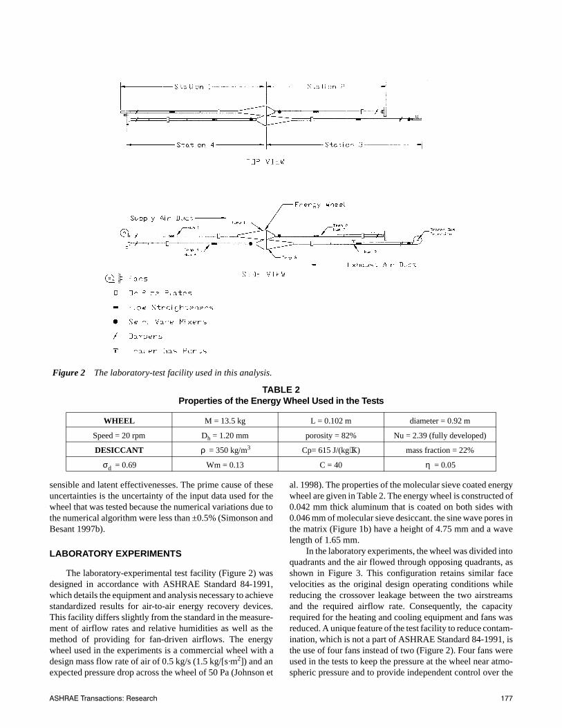
LABORATORY EXPERIMENTS

The laboratory-experimental test facility (Figure 2) wasdesigned in accordance with ASHRAE Standard 84-1991,which details the equipment and analysis necessary to achievestandardized results for air-to-air energy recovery devices.This facility differs slightly from the standard in the measure-ment of airflow rates and relative humidities as well as themethod of providing for fan-driven airflows. The energywheel used in the experiments is a commercial wheel with adesign mass flow rate of air of 0.5 kg/s (1.5 kg/[s·m2]) and anexpected pressure drop across the wheel of 50 Pa (Johnson et

al. 1998). The properties of the molecular sieve coated energywheel are given in Table 2. The energy wheel is constructed of0.042 mm thick aluminum that is coated on both sides with0.046 mm of molecular sieve desiccant. the sine wave pores inthe matrix (Figure 1b) have a height of 4.75 mm and a wavelength of 1.65 mm.

In the laboratory experiments, the wheel was divided intoquadrants and the air flowed through opposing quadrants, asshown in Figure 3. This configuration retains similar facevelocities as the original design operating conditions whilereducing the crossover leakage between the two airstreamsand the required airflow rate. Consequently, the capacityrequired for the heating and cooling equipment and fans wasreduced. A unique feature of the test facility to reduce contam-ination, which is not a part of ASHRAE Standard 84-1991, isthe use of four fans instead of two (Figure 2). Four fans wereused in the tests to keep the pressure at the wheel near atmo-spheric pressure and to provide independent control over the

TABLE 2 Properties of the Energy Wheel Used in the Tests

WHEEL M = 13.5 kg L = 0.102 m diameter = 0.92 m

Speed = 20 rpm Dh = 1.20 mm porosity = 82% Nu = 2.39 (fully developed)

DESICCANT = 350 kg/m3 Cp= 615 J/(kg⋅K) mass fraction = 22%

= 0.69 Wm = 0.13 C = 40 = 0.05

ρ

σd η

Figure 2 The laboratory-test facility used in this analysis.


initial rule set is set up for a controlled plant with assumedproperties (quick response or slow response). Then theSTFLC will improve itself to obtain optimal behavior. Adashed curve AB in Figure 2a indicates a performance trajec-tory deviating a little bit from the desired path such that it willenter into the left-half part of the linguistic plane, resulting inoscillation and overshoot. The dashed curve AC indicates aperformance trajectory deviating to the other side of thedesired path. The key objectives of the self-tuning strategyproposed in this study are to measure the deviation of theperformance trajectory from the desired one and to improvethe relevant rules or scale factors to eliminate the deviation.

In real applications, the desired performance trajectory isestablished based on operating experience and knowledge aboutfuzzy logic systems. In this work, the desired trajectory for theheating mode, shown in Figure 2a with AO, goes from point A topoint D where the derivative error (d) has a large value that resultsin the controlled parameter (T) responding quickly. Then thesystem approaches the stable point O along a smooth path.

The whole performance trajectory can be divided into fourstages located in four areas marked 1, 2, 3, and 4 in Figure 2a.In area 1, point E is chosen as a reference point and the perfor-mance is then measured by the distance de, which is defined asthe shortest distance from point E to the smoothed trajectory. Asmaller de results in a slower dynamic response, while a largerde results in a faster response in the first stage. In area 2, pointF is chosen as a reference point and the performance in thesecond stage then can be measured by the distance df betweenpoint F and the trajectory. In this area, a smaller df results in afaster dynamic response, while a larger df results in a slowerresponse. A very small df may result in overshoot in thedynamic process. Using the same analysis, points G and H arechosen as the reference points for areas 3 and 4, respectively,and dg and dh are used as the criterion to measure the perfor-mances of the STFLC in the third and fourth stages. Larger dgand smaller dh can lead to static error where the derivative ofthe error goes to zero before the error does. The performancemeasurement strategies are summarized in Table 1.

MODIFICATION PROCEDURE

There are two types of modification strategies: modifyingthe fuzzy subsets of the control rules or modifying theelements of the look-up table.

Replacing an old fuzzy control rule with a new one resultsin revising the fuzzy relation matrix. This involves detailedfuzzy mathematical calculations. If an old control ruleexpressed as a fuzzy matrix Rk,old (Huang and Nelson 1994a,1994b) is replaced by a new rule expressed as a fuzzy matrixRk,new, the general relation matrix Rg can be revised as

(1)

where Rk,old is the fuzzy complementary matrix of Rk,old. Thecomplementary operation on Rk,old and the intersection oper-ation with Rg,old signify “elimination” of the obsolete rulefrom the general relation matrix. The union operation withRk,new signifies “appending” the new rule to the general rela-tion matrix. Modifying fuzzy control rules is time-consumingand demands substantial computer storage.

For a given set of control rules, the control policy isusually expressed by a control surface (Huang and Nelson1994a, 1994b), which is expressed in terms of fuzzy subsets.Each cell in the control surface indicates the fuzzy value of thecontrol action. Figure 3a presents the control surface for acontrol rule set in terms of fuzzy subsets. A control surface canalso be expressed in terms of the elements of a look-up table.

TABLE 1 The Performance Measurement Strategies

for the Proposed STFLC

Stage Reference Criterion Smaller Value Larger Value

1 E de Slow response Possible overshoot

2 F df Possible overshoot

Slow response

3 G dg Overshoot Static error

4 H dh Static error Overshoot

Rg new, Rg old , Rk old,∩[ ] Rk new,∪=

(a)

(b)

Figure 3 Two types of control surfaces for a fuzzycontrol rule set: (a) control surface in terms offuzzy subsets; (b) control surface in terms ofelements.


airflow pattern and air turbulence in rooms. The flow patternsand air turbulence are generated primarily by air jets andsecondarily by internal heat loads. These effects are dependenton the temperature of the supply air. There is an extensivebody of literature concerning chilled air distribution, but thereis very limited information available on indoor airflow andtemperature measurements for cold air distribution systems.

Knebel and John (1993) conducted several field tests andshowed that cold air can be successfully supplied to a room toproduce a comfortable indoor environment under most oper-ating conditions by using the nozzle-type diffusers. However,the performance of the associated jet and the resulting fieldvelocities and temperatures are not given. Kondo et al. (1995)performed a laboratory study for cold air distribution systemswith a multi-cone circular diffuser. They concluded that thereare only minor differences in velocity and temperature distri-butions between an 8°C (46°F) cold air system and a 13°C(55°F) conventional system with the same room temperature.However, substantial condensation and dumping wereobserved for the 8°C (46°F) cases. Shioya et al. (1995) studiedthe thermal comfort aspect of a cold air distribution systemusing a thermal mannequin. Their work indicates that circularceiling diffusers gave a higher degree of comfort than linearslot diffusers in a similar situation. However, selection andpositioning of the diffusers was critical to ensure that thediffused air velocity remained satisfactory. Hassani and Stetz(1994) investigated the effect of local loads on the behavior ofcold air jets with early separation using an infrared visualiza-

tion technique to record the temperature distribution. Knapp-miller and Kirkpatrick (1994) and Kirkpatrick andKnappmiller (1996) have used the computational fluiddynamics (CFD) technique to study cold air jet behavior andthe associated indoor thermal comfort index. Rose andSeymour (1993) have provided some guidance as to the bestimplementation of cold air distribution with slot-type diffusersusing CFD analysis. Shakerin and Miller (1995) tested twotypes of vortex diffusers under isothermal conditions. Some-what more induction was observed compared with that of amulti-cone circular diffuser in their study.The authors areunaware of any other work on the subject of high-inductioncold air jets and their associated room air distribution pattern.

The objectives of the study described here were, there-fore, (1) to study the flow pattern and temperature distributionof nonisothermal jets issuing from a multi-cone circular ceil-ing diffuser, a nozzle-type diffuser, and a vortex diffuser, (2)to compare the performances of these diffusers and the asso-ciated room thermal comfort index under the condition ofsupplying cold air, and (3) to provide some useful suggestionsfor modifying the currently available multi-cone circular ceil-ing diffuser to fit the performance requirements of cold airdistribution.

EXPERIMENTAL SETUP

A full-scale environmental chamber 7.2 m (length) ×4.2 m (width) × 2.8 m (height) was constructed followingISO Standard 5219 (ISO 1984) and ASHRAE Standard 113

Figure 2 (a) Vortex diffuser, (b) multi-cone circular diffuser.

(b)

(a)


assumed for the theoretical calculation of the COP of absorptionheat transformers. The effectiveness of the intermediate heatexchanger was assumed to be 1.0. The work required to pumpthe strong solution and liquid working medium to the high-pres-sure side of the cycle is negligible. Heat losses to the surround-ings, as well as pressure drops due to friction, etc., wereassumed to be negligible.

In general, an absorption heat transformer is designed tofeed a large amount of exhaust heat at an intermediate tempera-ture level to the generator and evaporator as the driving heatsource and, at the same time, supply cooling water to thecondenser. It thus takes heat of higher temperature out of theabsorber by making use of the temperature difference betweenthe exhaust heat and the cooling water as the driving force. Figure1 shows a schematic diagram of a single-stage absorption heattransformer. Its coefficient of performance is expressed by thefollowing equation:

COP = QA/(QG+QE) = QA/(QA+QC) = 1/(1+QC/QA)

Operating Range

Figure 2 shows operating ranges for the various workingmedium+absorbent systems used. In comparison with theH2O+LiBr system, the H2O+LiBr+LiNO3 system showed awide operating range in the higher temperature range of thegenerator, which is concluded to have occurred because the solu-bility is larger for the latter system than for the former system inthe higher temperature range. The H2O+LiCl+LiNO3 systemshowed a narrow operating range in the lower temperature rangeof the generator due to the low solubility of this system. The oper-ating range shown by the H2O+LiI+LiNO3 system was some-what wide, even in the lower temperature range of the generator,and increased considerably with an increase in the temperature of

the generator. This is concluded to have occurred because thesolubility of this system is high even in the lower temperature rangeand is still higher in the higher temperature range. The systemsH2O+Ca(NO3)2+LiNO3, H2O+Ca(NO3)2+LiNO3+KNO3, andH2O+LiNO3+NaNO3+ KNO3 were found to have a narrow oper-ating range within the entire temperature range of the generator,compared with the H2O+LiBr system.

Figure 2 Comparison of operating range of various systems for single-stage absorption type.

Figure 1 Schematic diagram of single-stage absorption type.


Figure 4 Energy consumption using various compressors.

TABLE 4 Fresh Food Cycle Optimization Data (TL2.5F Compressor)

RefrigerantRefrigerant

Charge(g)

Temperature (°C)* Pressure (kPa)*EnergykWhd

Run Time% OnTff-a Tffe-i Tffe-o Pffcp-i Pffcp-o

R-134 111.60 7.67 0.41 7.45 248.15 732.35 0.76 5.18

125.70 7.72 2.39 7.14 246.34 743.40 0.63 5.90

145.60 7.87 3.70 5.62 233.44 750.41 0.60 12.39

161.70 7.96 4.11 4.06 225.62 787.29 0.63 22.41

179.30 7.93 4.30 3.65 225.90 783.19 0.62 23.18

201.30 7.92 4.42 3.28 228.69 796.08 0.79 31.25

R-227ea 139.50 7.67 −0.48 7.54 223.45 617.07 0.80 3.47

164.30 7.75 2.71 7.00 227.84 628.94 0.70 4.97

182.70 7.86 4.22 4.95 227.51 647.91 0.66 6.58

201.90 7.91 4.48 3.97 223.22 654.38 0.67 8.64

228.10 7.87 4.89 3.38 218.04 664.26 0.68 12.03

R-134a 159.00 7.70 3.55 4.26 272.86 1005.37 0.58 20.49

100.20 7.61 −1.96 7.69 219.88 945.78 0.84 14.36

118.40 7.63 1.12 7.64 222.22 980.50 0.67 26.62

140.40 7.63 2.95 5.55 254.99 994.00 0.60 21.95

189.10 7.81 3.64 3.60 281.68 1014.85 0.64 22.28

174.10 7.74 3.57 3.69 276.07 1014.85 0.61 21.23

216.90 7.85 3.83 3.26 294.06 1043.76 1.01 33.70

* fz = freezer, ff = fresh food, a = average, i = in, o = out, e = evaporator, cp = compressor, kWhd = kWh/day.


level, (K⋅A)drop, is evaluated by assuming the Lewis equationas unity approximately (Bernier 1995) as follows:

(22)

where Wi,av is the moisture content of the saturated air, whichis evaluated at Tw. Cpm indicates the average specific heat ofthe moist air, in J/(kgda⋅K), which can be determined asfollows:

. (23)

Finally, the coefficient of performance of the countercur-rent cooling towers (the available NTU) can be predicted byadding Equation 21 into Equation 22:

. (24)

On the other hand, the thermal demand equation (Ünsaland Varol 1990) can be revised by considering the evapora-tion, and a simple prediction formula for the sizing of thecountercurrent cooling tower can be written by consideringthe evaporation as follows:

(25)

The required NTU calculated by this formula indicates arealistic thermal demand for a specific cooling duty.

EXPERIMENTAL SETUP

A bench-top laboratory cooling tower of the vertical typewas used to conduct experiments for determination of thecoefficient of performance of the countercurrent cooling

tower shown in Figure 2. The cooling tower had fill charac-teristics, a, of 110 (m2/m3). The entering water mass flow raterange, mw,1, was between 0 kg/s and 0.05 kg/s. The coolingload was generated by an electrical resistance heater selectorof 0.5 kW, 1 kW, and 1.5 kW. Temperature was recorded by a0.1°C sensitive digital thermometer. The airflow rate wascontrolled by an air damper and measured by a venturimeter.The maximum dry airflow rate was approximately 0.06 kg/sdepending on the moisture content and specific volume of themoist air exiting the cooling tower. The water flow rate wascontrolled by a throttle valve and measured by an orificemeterwith a sensitivity of 0.001 kg/s. Makeup water was supplied bya tank, and the water level in the cooling tower water circula-tion tank was kept constant to achieve steady state in the cool-ing circuit. The wet-bulb temperature of the air was keptconstant during the experiments.

The actual available NTU of the cooling tower wasobtained by performing a series of experiments using theCarey-Williamson Method (Gurner and Cotter 1977) as

, (26)

where the corrected enthalpy driving potential, ∆im, isexpressed as follows:

(27)

and

(28)

where f is the correction factor of the arithmetic mean of theenthalpy driving potential, γm (see Figure 3).

Mean value of the saturated air enthalpy is evaluated at thearithmetic mean of the inlet and exit water temperatures. Meanvalue of the air enthalpy is evaluated at the arithmetic mean ofthe tower inlet and the exit air wet-bulb temperatures. f can beevaluated from the Carey and Williamson chart (Gurner andCotter 1977) as a function of the enthalpy driving potential atthe inlet and the exit states of the cooling tower, which are

(29)

(30)

K Ai⋅( )drop

0.5 mev⋅0.001 Cpm Wi,av Wav–( )⋅ ⋅------------------------------------------------------------------=

Cpm Cpa Wav Cpv⋅+=

NTUav

K Ai⋅( )total

mw,1---------------------------

K Ai⋅( )fill

K Ai⋅( )drop

+

mw,1---------------------------------------------------------= =

NTUreq

M2

M1-------

Cpw

n 1–( )---------------- 1n 1

i2 i1–( ) n 1–( )⋅ii ,1 i1–

----------------------------------------+

⋅ ⋅=

Figure 2 Schematic representation of the cooling towerused in the experiment.

NTUav

Cpw Tw,2 Tw,1–( )⋅∆im

-----------------------------------------------=

∆im f γm⋅=

γm ii,m im–=

Figure 3 Diagram of enthalpy driving potential.

γ1 ii ,2 i2–=

γ2 ii ,1 i1–=


Ql = heat generated by the overhead lighting,

Qex = heat from exterior walls and windows and the transmitted solar radiation.

Since there is a temperature stratification in a room withdisplacement ventilation, the ceiling and floor surface temper-ature are unknown. In this investigation, we use the twotemperatures in the CFD program to calculate the air temper-ature and contaminant distributions. Following is a discussionof a procedure used to estimate the temperatures.

In a space with displacement ventilation as shown inFigure 6, the steady-state heat balance on the surfaces of thefloor and the ceiling can be expressed as

Qaf = Qsf + Qrf + Qof, (6)

Qac = −Qsc + Qrc + Qoc , (7)

where

Qaf = convective heat transfer from the floor to the air,

Qsf = radiative heat transfer from the heat sources to the floor,

Qrf = radiative heat transfer from the ceiling and walls to the floor,

Qof = heat transfer from the space under the floor to the floor surface,

Qac = convective heat transfer from the air to the ceiling,

Qsc = radiative heat transfer from the heat sources to the ceiling,

Qrc = radiative heat transfer from the ceiling to the walls and floor,

Qoc = heat transfer from the ceiling surface to the space above the ceiling.

Further, Newton’s law reads:

Qaf = αcf (Tfs − Tf)A, (8)

Qac = αcc (Tc − Tcs)A, (9)

where

αcf = convective heat transfer coefficient on the floor,

Tfs = floor surface temperature,

Tf = air temperature near the floor,

αcc = convective heat transfer coefficient on the ceiling,

Tcs = ceiling surface temperature,

A = floor/ceiling area.

The convective heat transfer on the floor causes an airtemperature increase from the supply temperature to the airtemperature on the foot level. Therefore,

Qaf = ρCp V(Tf − Ts). (10)

The radiative heat transfer from the heat sources to thefloor and the ceiling, respectively, may be estimated by

, (11)

, (12)

where

Qj = heat emitted by jth heat source, including transmitted solar radiation;

rfj = fraction of radiative heat transfer from jth heat source to the floor;

rcj = fraction of radiative heat transfer from jth heat source to the ceiling.

The rfj and rcj need to be estimated from the room geometry.

According to Mundt (1996), the radiative heat transferfrom the ceiling and walls to the floor, Qrf, and the radiativeheat transfer from the ceiling to the floor and walls, Qrc, canbe estimated via

Figure 6 Heat transfer in a space with the displacement ventilation.

Qsf rfjQjj

∑=

Qsc rcjQjj

∑=


level and IAQ are statistically significant (p-values <0.05).These trends were obtained through analysis of a sample ofoffice buildings in the Chicago metropolitan area. However,the trends indicate similarities throughout the United Statesand Canada. The statistical analysis also recognized the factthat larger buildings typically have more components andwould have higher O&M levels. This was accomplishedthrough a statistical comparison of IAQ information fromsmall and large buildings, which was independent of size,outdoor ventilation rates, and space temperature.

STANDARD SOP STRUCTURE

A standard SOP structure was developed to ensureconsistency. Three levels of SOPs were developed:

• Building

• System

• Component

The system level will generally be sufficient for mostbuildings; however, complex buildings may also require SOPsfor components and the whole building. The SOP develop-ment strategy and structure developed in the guide (Dorgan etal. 1998b) concentrate on the system level; however, the strat-egy and structure apply to all three SOP levels.

Information from O&M personnel and ASHRAE Guide-line 4-1993 provided the basis for the SOP structure. The SOPdocumentation consists of seven sections. The first sectionincludes basic information on the system, building, or compo-nent being addressed. The other sections provide informationon how to evaluate and the correct action to take if required.

Section 1: General Information

This section provides a short description of the building,system, or component to be addressed in the SOP. Document-ing the Design Intent provides an important resource forunderstanding system operation and limitations. System SOPinformation contained in this section includes:

• System type• Area served• Control description• Associated systems or components

Section 2: Standards of Performance

The criteria used to evaluate the SOPs are developed inSection 2. The evaluation process meets the SOP requirementof ensuring that “a building, system, or component is operat-ing properly —determined through a series of measurements.”The criteria may be taken from existing standards (ASHRAEfor example), local codes/guidelines, or manufacturer’s infor-mation. The criteria may be measured or subjective. The crite-ria used for evaluation vary by season (summer/winter) or byoccupancy mode (unoccupied/occupied). Examples of SOPcriteria are:• The energy efficiency for a chiller is less than 0.6 kW/ton

(0.017 kW/kWT) full load and 0.7 kW/ton (0.020 kW/kWT) at 50% load.

• The IAQ in a conference room meets the requirementsof ANSI/ASHRAE Standard 62-1989 for CO2 levels.

Section 3: Information to be Recorded

Measurements must be taken to determine if SOPs aremet. The validity and usefulness of the measurements requirethat the frequency, accuracy, number, references, and otherdetails be determined.

An example of the measurements required for the chillerEER SOP discussed in Section 3 are:

• Entering and leaving chilled-water temperatures• Chilled-water flow rate• Energy input

The same measurements can be used in more than oneSOP, which allows for the actual list of required measurementsto be reduced.

Section 4: Calculations

The measurements are used to ascertain that the SOPs arebeing met. This is accomplished through calculations involv-ing the information recorded in Section 3. Calculations may beeasily automated through computerized scheduling and track-ing systems.

Equation 1 is an example of a calculation for determiningthe chiller EER.

Figure 2 IAQ/O&M trend.

396 ASHRAE Transactions: Symposia

area is very large as is the case for open plan offices, andenclosed rooms are ones that are relatively small with wallslike those of private offices. For these rooms, the fire locationsand the arrangements of HVAC supplies and returns are shownin Figure 1.

MODELING APPROACH

A commercially available computational fluid dynamics(CFD) model was used to perform the numerical simulations.This model (CFC 1995) is an upgrade of the one used for simu-lations in the second year of this project, and the only upgradedfeatures relevant to the simulations of this study consist ofsimplified data input.

A detailed description of CFD modeling is beyond thescope of this report. The nonmathematical descriptions in thefollowing sections are intended to provide an explanation ofthe assumptions of the simulations of this paper and to provideinsight for those not familiar with the field. The user’s manual(CFD 1995) provides the exact equations and mathematicaldefinitions that apply to these simulations. For more informa-tion about CFD modeling, readers are referred to Abbott andBasco (1989), Anderson et al. (1984), Hirsch (1990), Hoff-

mann (1989), and Kumar (1983). For general informationabout fluid dynamics, readers are referred to Schetz (1993),Schlichting (1960), Sherman (1990), White (1974), and Yuan(1967).

CFD Concept

The CFD modeling consists of dividing the flow field intoa collection of small rectangular cells and determining theflow at each cell by numerically solving the governing conser-vation equations of fluid dynamics. Boundary conditions areprescribed for walls, floor, ceiling, HVAC supplies, HVACreturns, openings to the outside, and planes of symmetry. Forthis project, all the CFD simulations were unsteady, using thecalculated properties from one time step to calculate those ofthe next time step. At the start of a simulation, each cell can beset to zero flow conditions or conditions read into thecomputer from a previous simulation. Zero flow conditionsconsist of zero velocity and ambient pressure and temperature.To generate fire-induced flows, heat is released in severalcontrol volumes over time.

The governing equations of fluid dynamics describe themotion of fluid throughout the flow field. These equations are

TABLE 1 Room Dimensions in Meters (Feet) for CFD Simulations

Room Type A B C D H

O1 4.6 (15) 4.6 (15) 9.2 (30) 9.2 (30) 2.74 (9.0)

O2 5.5 (18) 3.91 (13) 10.5 (34) 9.09 (30) 2.74 (9.0)

E1 4.6 (15) 4.6 (15) N/A N/A 2.74 (9.0)

E2 4.6 (15) 3.0 (9.8) N/A N/A 2.74 (9.0)

E3 4.6 (15) 1.71 (5.6) N/A N/A 2.74 (9.0)

E4 4.6 (15) 2.56 (8.7) N/A N/A 2.44 (8.0)

E5 6.0 (20) 2.3 (7.5) N/A N/A 2.44 (8.0)

ASHRAE Transactions: Symposia 411

ments for fixed guideway transit systems. NFPA 130 requiresemergency ventilation in stations and tunnels to protect thepassengers and employees from a fire or smoke generation.The criteria specified in the standard are as follows:

• The emergency ventilation system shall produce airflowrates to provide a stream of noncontaminated air to pas-sengers and employees in a path of egress away from atrain fire and to prevent back-layering of smoke in apath of egress away from a train fire.

• The maximum temperature in the path of evacuationshall not exceed 60oC, ignoring radiant heating effects.

• The air velocity in the path of evacuation shall notexceed 11 m/s; air velocities above this level may causedifficulty in walking.

To preclude imposing requirements on older existingtransit systems, which may be impractical and/or cost prohib-itive, NFPA 130 does not mandate that existing systemscomply with these ventilation requirements. Almost all of theBuenos Aires Metro was built long before NFPA 130 wasissued. The system has for many decades provided safe andreliable service. Major fires that would require ventilationsystems to assist passenger safety have been rare over thehistory of the transit system. However, Buenos Aires Metroplans to improve the subway ventilation based on NFPA 130with priority given to meeting the requirements for low-inten-sity fires throughout the subway system. For new subwaysystems, recommendations are for the high-intensity fire of atrain fully engulfed in fire.

Fire Heat Release Rate

The train fire heat release rate used for the analysis was alow-intensity fire of 1.8 MW (NYC 1994). This value corre-sponds to a train fire that involves only the undercar combus-tible contents.

VENTILATION ALTERNATIVES

The analysis of alternative ventilation strategies focusedinitially on identifying and evaluating the potential use of vari-ous strategies that have been used successfully in the industry.These strategies include (1) end-of-station fan plants, (2) mid-tunnel fan plants, (3) propeller fans, (4) jet fans, and (5) stationmechanical ventilation. In evaluating these strategies, carefulconsideration was given to space constraints for locatingequipment within and around the stations, cost-effectiveness,and feasibility. The strategy that would best meet all criteriawas the jet fan option. The recommended system consists ofjet fans in the tunnels generally located 50 meters from eachend of the stations. The jet fan operating mode would bedependent on the location of the fire within the station.

CFD ANALYSIS

A CFD analysis was performed using a commerciallyavailable CFD software, run on a DEC Alpha workstation. For

the last five years, the SES program has been used in conjunc-tion with CFD to simulate fire emergencies in subway stationswhere three-dimensional modeling is more appropriate. WhileCFD has the capability to model more complex station geom-etry, the SES program provides the fundamental boundaryconditions necessary for the CFD analysis. This coupling ofcomputer tools has helped subway ventilation engineers tosolve problems and analyze situations where conventionaltechniques would have failed or been grossly inadequate.

CFD simulations were performed to evaluate the stationconditions resulting from a fire on board a train stopped in astation with and without mechanical ventilation. For naturalventilation (i.e., no mechanical ventilation), ambient pressurewas assumed at all flow boundaries. For mechanical ventila-tion, simulations were performed to determine the airflowboundary conditions at the ends of the station. Ambient pres-sure conditions were used at station entrances.

Two stations were selected for the simulations: Medrano Station is a cut-and-cover station with side plat-

forms and no mezzanine. The station is about 130 m long, 33 mwide, and 6 m high. The station has a total of four exits. Eachplatform has two exits to outside ambient. Figure 1 shows thegeneral layout of the station. The computational grid used forthis station is about 84,000 cells. The grid consists of 117 cellsin the longitudinal x-direction, 20 cells in the vertical y-direc-tion, and 36 cells in the lateral z-direction. The number of cellsis based on previous project experience with consideration ofthe accuracy required in the study.

Pueyrredon Station is a bored tunnel station with a mezza-nine above the two side platforms. The station is about 130 mlong, 21 m wide, and 10 m high. Two escalators and one stair-way connect each platform to the mezzanine. This station hasfive exits. Figure 2 shows the general layout of the station. Thecomputational grid used for this station was about 85,000cells. The grid consists of 131 cells in the longitudinal x-direc-tion, 21 cells in the vertical y-direction, and 31 cells in thelateral z-direction.

Two fire scenarios were considered: (1) a fire at either endof the station beyond the last exit or staircase and (2) a fire

Figure 1 Medrano station layout. Grid (117 × 20 × 36).


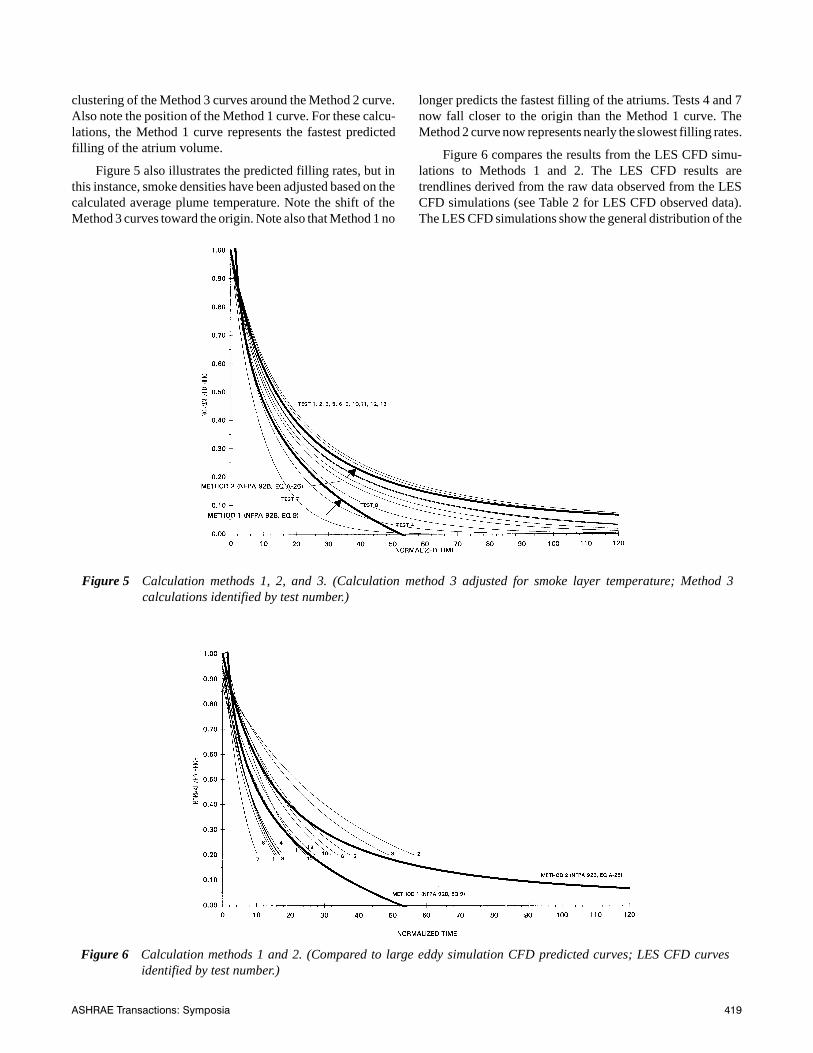
clustering of the Method 3 curves around the Method 2 curve.Also note the position of the Method 1 curve. For these calcu-lations, the Method 1 curve represents the fastest predictedfilling of the atrium volume.

Figure 5 also illustrates the predicted filling rates, but inthis instance, smoke densities have been adjusted based on thecalculated average plume temperature. Note the shift of theMethod 3 curves toward the origin. Note also that Method 1 no

longer predicts the fastest filling of the atriums. Tests 4 and 7now fall closer to the origin than the Method 1 curve. TheMethod 2 curve now represents nearly the slowest filling rates.

Figure 6 compares the results from the LES CFD simu-lations to Methods 1 and 2. The LES CFD results aretrendlines derived from the raw data observed from the LESCFD simulations (see Table 2 for LES CFD observed data).The LES CFD simulations show the general distribution of the

Figure 5 Calculation methods 1, 2, and 3. (Calculation method 3 adjusted for smoke layer temperature; Method 3calculations identified by test number.)

Figure 6 Calculation methods 1 and 2. (Compared to large eddy simulation CFD predicted curves; LES CFD curvesidentified by test number.)


also serves as the heat pump that both entrains air into theactive combustion zone and then circulates the combustionproducts through the surrounding enclosure. It is the latter rolethat is of interest here. Although the central role of the fireplume has been recognized for some time, there is still muchuncertainty about the plume structure. Indeed, Zukoski (1994)gives a recent summary of the state of knowledge of massentrainment into isolated fire plumes. There is clearly noconsensus on any simple formula or graphical correlation forthis most basic of plume quantities. Much of this uncertaintyarises from the experimental and conceptual difficulty associ-ated with determining the outer plume boundary. McCaffrey(1979) developed centerline mean velocity and temperaturecorrelations that are consistent with a large body of experi-mental data (Baum and McCaffrey 1989).

To perform a computational study of an isolated fireplume, the minimum length scale that must be resolved is theplume structure scale.

(15)

is roughly comparable to the plume diameter near thebase. It involves the heat release rate Q directly and can beseen both in the dimensionless form of McCaffrey’s plumecorrelations and by considering the dimensionless form of theNavier-Stokes equations for this problem. In fact, if the equa-tions discussed above are made nondimensional with aslength scale, as velocity scale, as time scale,and T0 as temperature, all the physical constants disappearfrom the inviscid terms in the equations. Only Reynolds andPrandtl numbers appear in the viscous stress and heat conduc-tion terms.

In order to simulate the convective mixing of the fire plume,the grid spacing should be about 0.1 or less. Figure 1 showsan instantaneous snapshot of three temperature contoursobtained from a 96 × 96 × 96 cell simulation. The contourscorrespond to the boundaries of the continuous flame, inter-mittent flame, and plume zones as defined by Baum andMcCaffrey (1989). Note that the image is an instantaneoussnapshot of the fire and that time averages of the output of thiskind of simulation must be produced in order to make quan-titative comparison with most experimental data. Indeed, it isthe fact that the results of the simulation can be averaged in aroutine way while the equations of fluid mechanics cannot thatis the basis of the whole approach presented here.

On the left of Figure 2 are the instantaneous verticalcenterline velocity and temperature profiles superimposed onthe steady-state correlation of McCaffrey (circles). The oscil-lations are primarily due to the large toroidal vortices gener-ated at regular intervals at the base of the fire, which then riseasymmetrically. Note that the flow is not even remotely axiallysymmetric and the centerline is defined only by the geometryof the pool at the base of the plume. The right side of Figure2 shows the corresponding time-averaged quantities (solidlines) and McCaffrey’s centerline correlations. The time-aver-

aged flow is symmetric and in excellent agreement with thecorrelations. The major deviations are at the bottom of theplume, where the thermal elements are turned on instanta-neously without any preheat as they leave the pool surface.Otherwise, the boundaries of the computational domain areopen. At these open boundaries, the perturbation pressure isassumed zero. This is a reasonable approximation at the sideboundaries but less so at the top. Various strategies have beenexplored to properly set the conditions at the top, but in mostinstances, there is usually a solid ceiling or a hood drawing thecombustion products up at some specified flow rate. Figure 3shows the corresponding radial dependence of the verticalvelocity and temperature at heights of = 2.8 (intermittentregion) and = 5.3 (plume region). The results of thesimulation are compared with Gaussian profiles that incorpo-rate the half-widths obtained from McCaffrey’s correlations.

D∗ Q ρ0cpT0 g⁄( )2 5⁄

=

D∗

D∗gD∗ D∗ g⁄( )

D∗

Figure 1 Instantaneous snapshot of a pool firesimulation performed on a 96 × 96 × 96 grid.The contours correspond roughly to theboundaries of the continuous flame,intermittent region, and plume. The squareburner is of length D* with the height of thecomputational domain rising to about 12 D*.

z D∗⁄z D∗⁄


The borehole shape factor data (Figure 2) and the associatedcurve fit relations (Equation 3 and Table 1) provide a conve-nient method for calculating effective grout thermal resistancefor any bore size, pipe size, grout thermal conductivity, andassumed pipe spacing that are commonly encountered in prac-tice.

Currently, when U-bend heat exchanger loops areinstalled in boreholes, they are simply weighted and sunk orpushed into the borehole. No control over the pipe spacing inthe borehole is available. Therefore, an assumption must bemade about the average pipe spacing in the borehole before theeffective grout thermal resistance can be estimated. The Aconfiguration is a conservative design assumption and shouldonly be considered when large uncertainties exist in the forma-tion thermal conductivity. The B configuration would be anappropriate design assumption in most situations, as it repre-sents an average spacing along the entire borehole length. Thisassumption would be most appropriate if reliable informationis available on the formation thermal conductivity. Configu-ration C would never consistently occur in practice and is arisky design assumption that could lead to underdesigned looplengths. Even with very good formation soil thermal conduc-tivity data, a device to ensure this spacing with a very highlevel of certainty would be required before this level of perfor-mance could be realized.

Borehole thermal resistance can be found knowing thatthe effective grout thermal resistance and the pipe thermalresistances act in series, as shown in Figure 3. The total piperesistance is equivalent to the thermal resistance of two indi-vidual pipe thermal resistances in parallel. Assuming that thefluid temperatures in each pipe are the same, the equation tocalculate the equivalent thermal resistance of two pipes inparallel follows:

(4)

Since the two pipe resistances are equal (Rp1 = Rp2 = Rpipe),Equation 4 reduces to

. (5)

Then, the borehole resistance (excluding convectionresistance on the inside pipe wall) can be found by adding theeffective grout thermal resistance to the parallel pipe thermalresistance:

. (6)

Pipe thermal resistances and parallel pipe thermal resis-tances for common pipe diameters and dimension ratios usedfor vertical heat exchanger U-bends are provided in Table 2(IGSHPA 1988).

Field Tests

The thermal responses of various boreholes with differentdiameters, depths, pipe sizes, and grout types were measuredby Austin (1998), Smith (1997), and Remund (1997). Theprocedure consisted of rejecting a known rate of heat into the

TABLE 1 Curve Fit Coefficients for

Shape Factor Correlation in Equation 3

Configuration β0 β1

Correlation Coefficient

A 20.10 −0.9447 0.9926

B 17.44 −0.6052 0.9997

C 21.91 −0.3796 0.9697

Figure 2 Borehole shape factor relations for thermalresistance pipe configurations.

Figure 3 Parallel-series model for pipe thermalresistance and effective grout thermalresistance.

Rpp

Rp1Rp2

Rp1 Rp2+------------------------=

Rpp

Rpipe

2-------------=

Rb Rpp Rg+=


ABSTRACT

Optimal performance of closed-loop, ground-source heatpumps (ground-coupled heat pumps) is dependent upon thethermal properties of the backfill in the annular regionbetween the ground heat exchanger (GHEX) tubes and theouter bore wall. Equally important is the protection of ground-water aquifers from contaminants that may flow from thesurface or other aquifers through poorly sealed boreholes.Conventional cement and bentonite-based grouts have rela-tively low thermal conductivities. Loop requirements oftenincrease beyond the allotted budget in applications whereregulatory bodies require the entire heat exchanger length tobe grouted.

This paper reports on the results of four mixes of thermallyenhanced cementitious grouts. Four grouts were evaluated ina test stand to minimize the impact of external factors typicallypresent in field tests. The test stand accepts up to 6 in. (15 cm)ground heat exchangers in a 10 ft (3 m) test section. Controlledtesting is performed in either the cooling mode (loop above85°F [29°C]) or heating mode (loop at 32°F [0°C]), and thetemperature of the outer bore wall is held constant with agroundwater source.

Results indicate cement grouts that are enhanced with low-cost additives have thermal conductivities three to four times aslarge as conventional high-solids bentonite grouts. This wouldresult in reduced heat exchanger lengths compared to thosegrouted with bentonite. There appears to be no measurableincrease in overall borehole resistance due to separation of thecolder tubes from the grout in the heating mode. This discussiondoes not include pumpability, permeability, and materialhandling issues, which must be thoroughly investigated beforeany grout can be recommended for use.

INTRODUCTION

The vertical ground heat exchanger (GHEX) is an impor-tant component in a ground-coupled heat pump (GCHP)system. The design must balance the constraints of high ther-mal performance, reasonable cost, durability, and ease ofinstallation. An additional constraint must be imposed in orderto ensure that these systems maintain their positive environ-mental advantage. This requirement is to prevent contami-nated surface water or water from a poor quality aquifer fromentering into drinking water or irrigation aquifers.

Figure 1 demonstrates the components of three situationsencountered in the installation of vertical U-tube GHEXs. A3.5 in. to 6 in. (9 cm to 15 cm) diameter bore is drilled in the

Figure 1 Hydrogeological variations for GCHPU-tube heat exchangers.

Testing of Thermally Enhanced Cement Ground Heat Exchanger Grouts

Stephen P. Kavanaugh, Ph.D. Marita L. Allan, Ph.D.Member ASHRAE

Stephen P. Kavanaugh is a professor of mechanical engineering at the University of Alabama, Tuscaloosa. Marita L. Allan is a scientist atBrookhaven National Laboratory, Upton, N.Y.

CH-99-2-2


bore) to some extent, which has the effect of enhancing theborehole thermal conductivity. This feature is considered to bethe primary reason for the higher performance.

According to theory, borehole 1 should have a lower pseudo-resistance profile than borehole 3 because the same grout wasused in a 4.5 in. (0.114 m) borehole as in a 6 in. (0.152 m) one.Use of the thermal resistance method, shown in Figure 4,produces the results expected. Although the two curves forboreholes 1 and 3 in Figure 4 are not separated by a largeamount, they are distinctly separate, and the greater the differ-ence between the formation thermal conductivity and the groutthermal conductivity, the greater the difference would bebetween curves such as no. 1 and no. 3.

The curves shown in Figure 4 for boreholes 2 and 4converge. Temperature and time at this site were used to deter-mine the average thermal conductivity of the formation fromthe five boreholes and resulted in a value of 1.079 Btu/ft⋅h⋅°F(1.867 W/m⋅°C); the measured grout thermal conductivityused in boreholes 2 and 4 is 0.85 Btu/ft⋅h⋅°F (1.471 W/m⋅°C).Since the grout and formation thermal conductivity are closeto the same, it is expected that borehole diameter would notsignificantly change the thermal resistance values. This isapparent when noting that borehole 2 is 4.5 in. (0.114 m) indiameter and borehole 4 is 6 in. (0.152 m) in diameter, but thecurves in Figure 4 are essentially the same. The relative posi-tions of the curves in Figure 4 demonstrate that enhanced groutperforms significantly better than standard bentonite grout.

CHARACTERISTICS OF BARTLESVILLE, OKLAHOMA, TEST BOREHOLES

Seventeen boreholes were drilled in a single field toprovide energy for a convenience store in Bartlesville, Okla-homa. DOE provided funding to complete and evaluate theperformance of the last four. These are in a line at the end ofthe field of heat exchanger loops. Boreholes 16 and 17 werecompleted with 63.5% solids-enhanced grout, the same as intest sites described previously. Borehole 15 was completedwith 30% solids bentonite grout, which was used at two of thepreviously described sites. Boreholes 1 through 14 were

completed with a native Oklahoma sand-bentonite mix (nativeEG) with a portion of cement added. This was the first timethat a bulk mixture of this type was tested for field perfor-mance.

The distribution of the curves (Figure 5) among boreholes15, 16, and 17 is as expected from a theoretical viewpoint.Borehole 15 is bentonite-grouted and of the same diameter asall the others except no. 17, which is a 4 7/8 in. (0.124 m) bore-hole. Because the grout thermal conductivity in borehole 15 islower, the pseudo-thermal resistance, as shown in Figure 5, ishighest. Borehole 17 contains enhanced grout, but the bore-hole diameter is greater, so the pseudo-thermal resistancewould be expected to be lower than that of holes filled withbentonite. Borehole 16, with 63.5% solids-enhanced grout anda smaller borehole, would provide a lower thermal resistance,as indicated in Figure 5. Because grout in borehole 14 isenhanced with sand, the pseudo-thermal resistance wasexpected to be lower than that of the bentonite-grouted bore-hole 15; however, its relation to the 63.5% solids-enhancedgrout was not predicted. Figure 5 shows that native Oklahomaenhanced grout performs in essentially the same manner in a3 5/8 in. (0.092 m) borehole as 63.5% solids-enhanced groutperforms in a 4 7/8 in. (0.124 m) borehole. Since the largerborehole degrades the performance but the 63.5% solids groutperforms the same as the EG-enhanced grout, then the conclu-sion is that the 63.5% solids grout performs better than the EG-enhanced grout.

Contrary to results of the South Dakota tests, comparisonof effects of enhanced grout with changes in borehole diame-ter at Bartlesville shows a distinct difference between the two63.5% solids grout tests. The following hypothesis was veri-fied by tests of the two 63.5% solids-enhanced grouts: whereconductivities of grout are close to the formations’ thermalconductivities, borehole diameters will have no effect; wherea difference exists in the thermal conductivities, performancedegradation occurs as the borehole gets larger. Tests on thefour Bartlesville bores produced an average formation thermalconductivity of 1.68 Btu/ft⋅h⋅°F (2.907 W/m⋅°C), which isalmost twice the thermal conductivity of the grout—thus the

Figure 4 Pseudo-thermal resistance as a function ofcumulative power per depth of loop,Brookings, South Dakota.

Figure 5 Pseudo-thermal resistance as a function ofcumulative power per depth of loop at aconvenience store in Bartlesville, Oklahoma.


refrigerant used in the this study is R-22, whose thermody-namic and transport properties were evaluated using thecomputer program REFPROP (NIST 1997).

EXPERIMENTAL PROCEDURES

Initially, the test section was cleaned and checked forleakage before it was evacuated. Then the system was evacu-ated using a turbo-molecular vacuum pump. The vacuumpump continued working for another two hours after thevacuum gauge manometer reached 10-4 torr to ensure that itcontained no noncondensable gases. Before obtaining a seriesof experimental data for the boiling of mixtures with differentcompositions, the experimental setup was cleaned thor-oughly prior to filling the vessel with the refrigerant. Poolboiling experiments were conducted at saturation tempera-tures of −5°C, 4.4°C, and 20°C. The liquid refrigerant mixturewas gradually preheated to its corresponding saturated statebefore running each test. Power was then adjusted to a prede-termined value. The criteria for the steady-state conditionwere variation of system pressure to be within ±3 kPa andmean temperature variations of the wall surface less than±0.1°C over five minutes. All the data signals are collectedand converted by a data acquisition system (a hybridrecorder). The data acquisition system then transmits theconverted signals through GPIB interface to the host computerfor further operation. The experimental uncertainties reportedin the present investigation were analyzed following thesingle-sample method proposed by Moffat (1989). The maxi-mum and minimum uncertainties of the heat transfer coeffi-cients were estimated to be approximately 18.4% for = 3 Wand 3.5% for = 700 W.

DATA REDUCTION

The heat transfer coefficient for each power input wascalculated as follows:

(1)

where is the electric heating power and Ts is the saturationtemperature for pure refrigerant based on the measuredsystem pressure. The outside surface area, Awall, is evaluatedas πDol. Note that Do is the outside tube diameter, and l is theeffective length of the cartridge heater (the length of thecartridge heater is 100 mm). Twall is the mean average walltemperature at the outer surface, which can be calculated fromthe measurement of inside temperatures and is given by

(2)

where Twi is the arithmetic mean of three inside wall temper-atures:

(3)

where Tw1, Tw2, Tw3, and Tw4 are the inside wall temperaturereadings.

EXPERIMENTAL RESULTS

Figure 3 shows a comparison of heat transfer coeffi-cients and the predictions by the correlations from Cooper(1984) and Gorenflo (1993). As seen, the predictions by the

TABLE 1 Physical Properties of the Test Oils

TypeViscosity

(SUS/100ºF) Viscosity

(cSt/100ºF) Pour (ºF)

Pour (ºF)

Specific Gravity

Surface Tension (dynes/cm)

3GS 155 33 −40 −65 0.91 47

5GS 525 113.4 −10 — 0.918 40

Q·

Q·

)(

.

swallwallTTA

Qh

−=

Q·

lk

DDQTT

w

iowiwall

π2

)ln(.−=

4

4321 wwwwwi

TTTTT

+++=

Figure 3 Comparison of the R-22 plain tube data withcorrelations.


cial flooded evaporator units. Saturation temperatures of 40°Fand 80°F (4.4°C and 26.7°C) were used.

The presence of oil in a tube bundle has a significanteffect on the boiling process for both plain and finned tubing.With smooth brass tubes in a bundle, Cotchin and Boyd(1992) utilized R-113 with and without oil in a 60-row by 3-column bundle section. Electric cartridge heaters providedthe heat load and a pump circulated the refrigerant across 1 in.(25.4 mm) tubes. It was found that up to 20%, by volume, oilconcentration could increase the heat transfer. Using R-12,Danilova and Dyundin (1972) examined finned copper tubesin six rows. Negative performance effects are noted with 8%oil, by weight. The oil contamination reduced boiling coeffi-cients by 5% to 50%, depending on saturation temperature andheat flux, and had the greatest impact at the lower heat fluxes.Likewise, tube row performance variation is more pronouncedwith oil in the bundle.

Memory et al. (1995) examined R-114 and R-114/oilpool boiling using smooth, 19 fpi (Gewa-K), turbo-B, andhigh-flux surfaces. As expected, average bundle coefficientsimproved with oil content up to about 3% with the smooth andfinned tube types. Between 4% and 10%, the coefficientsdecreased somewhat; in all cases, there was improvement overthe no-oil case. The oil enhancement ranged from 20% to 60%over that of the pure R-114 fluid with the finned tubes; theplain, smooth tube case showed improvement of 20% to 40%.

Given the limited available information in the open liter-ature in conjunction with the use of alternative refrigerants, itbecomes necessary to provide added data, particularly forother refrigerants flow boiling in finned tube bundles. Thus,the focus of this study is the experimental determination of theeffects of oil on heat transfer with R-123 and R-134a with thistype of tube.

REFRIGERANT FLOW LOOP

The experimental setup is displayed, in schematic form,in Figure 1. It consists of a tube bundle test section, in whichthe refrigerant boiling takes place, within a pressure test cham-ber. The vapor refrigerant out of the tube bundle test section iscondensed by the two lower coils arranged in parallel and bythe presence of a third cooling coil located above the testsection, inside the test chamber. This heat is ultimatelyrejected by a nominal ten-ton, air-cooled external chiller thatcirculates a 40% (by weight) ethylene glycol/water solutionthrough the condenser coils. The chilled water solution rangesfrom 15°F to 25°F (−9°C to −4°C) depending on the total rateof heat rejection in the test section. From the lower condens-ers, the liquid is pumped through a bank of rotameters so thatthe flow rate can be measured. Liquid refrigerant can bedirected to any of four rotameters having capacities rangingfrom 3.67 gpm to 0.2675 gpm (13.89 L/min to 1.01 L/min) ofwater. The choice of rotameter is based upon the refrigerantmass flow rate to ensure mid-scale readings. The liquid streamis then passed through the in-line electric heater piping sectionto generate the appropriate amount of vapor (15% inlet vaporquality).

The heater is located in the liquid refrigerant line betweenthe rotameters and test section inlet. To prevent separation ofany oil from the two-phase refrigerant mixture, the heaterpiping is sloped upward so that the oil, vapor, and liquidremain well mixed and are carried to the test section. (Othertypes of separate boiler facilities would serve to concentratethe oil inside the facility, over time, as the vapor is produced.)The two-phase flow crosses a distributor plate and then passesupward, through the tube bundle in the test section, perpen-dicular to the axis of the tubes. Heat from the tube bundleconverts the two-phase mixture to vapor that exits the top of

Figure 1 Flow boiling test loop.


ho is found. At higher oil content, the difference between thetop and middle tubes and the bottom tube is magnified; thecoefficient can be three times greater for the upper tubes, asseen in Figures 12 and 13. Except for the bottom tube, at higheroil concentrations the heat transfer is relatively insensitive toheat flux, even decreasing slightly with qo.

Overall average oil effects are noted in Figure 14. The heattransfer is typically increased, based upon the pure R-134aboiling reference. At 1% oil, the results are mixed, with a slightdecrease at low qo and a small increase for qo > 5200 Btu/h⋅ft2

(16,404 W/m2). In the 2% to 7% oil range, ho can be 30% to70% larger, 50% being typical, than the no-oil case. At higheroil content, the heat transfer advantage appears to level off andmay begin to reduce near 10% oil. Table 2 contains all of theoil-related data for the R-134a. (Again, the location of each oilport is found in Figure 2.)

R-22 Data Trends

Figure 15 presents the R-22 experiments. Only pure R-22was tested in the bundle after the R-134a. Qualitatively, the

Figure 10 Individual 26-FPI/R-134a tube performancewith 0% oil.

Figure 12 Individual 26-FPI/R-134a tube performancewith 1% average oil.



2 CH-99-4-2

BACK TO PAGE ONE

despite improvements in technology, this remains quite a chal-lenge.

Interactions between air conditioning and refrigeratedcases influences energy consumption and sales parameters(food integrity and appearance, thermal discomfort).Besides thermal coupling, air carried in through front doorsand customer traffic is also a source of moisture. Displaycases continuously operate as heat and moisture traps.Because the freezer case (see Figure 3) evaporation temper-ature is near −35°C (−31°F) (vs. about 4°C [39°F] for arooftop air conditioner), when cases cool the indoors, it isenergy consuming. Furthermore, dehumidification indisplay cases is inefficient due to the additional energyrequired for defrosting and re-cooling cycles. The aim is todevelop a new approach to study this interaction and to lookfor an optimal indoor air condition, using real figures.

Literature Review

Although supermarket energy challenges are well set inAdams (1985), the interactions between refrigeration and airconditioning are often unknown or misunderstood. The tradi-tional separation of the air-conditioning and refrigerationindustries has limited exchange of design information. Never-theless, since the early 1980s, some progress has been made.For example, the development of efficient desiccant cooling inthe United States is described in Meckler (1992). The air in theentire supermarket is maintained at a low humidity. In France,another type of humidity control is currently being tested,which consists of supplying a very dry air curtain just behindthe display case (Bernet 1997).

Energy analysis is developed in Khattar et al. (1991)using the TRNSYS building simulation model. However, thisstudy is mostly based on detailed modeling of various refrig-eration components and on possible improvements of therefrigerating system. It gives no evidence of the interactionbetween air conditioning and refrigerated cases. A significantwork on the influence of indoor humidity on refrigerateddisplay case consumption is presented in Howell (1993a). Itconsiders two types of air curtains according to display casetypes (horizontal or vertical) in order to calculate heat andmoisture exchanges. The results are validated by experimentaldata. In Howell (1993b), regression equations are used to eval-uate heat and moisture transfers under any indoor relativehumidity for typical cases. Building simulation was used tosee the influence of the relative humidity control on air-condi-tioning consumption. Some typical ratios are given for a warmand humid climate (Tampa, Florida) in Howell et al. (1997): a5% reduction in store relative humidity gives a total storeenergy load reduction of nearly 5%. However, indoor temper-ature set-point influence was not studied in this paper. Anotherpoint is that supermarket dimensions in the United States arevery different from those in France, which influenced the deci-sion to make some appropriate simulations.

No modeling of the cold aisle phenomenon, which isessential in the analysis of coupling, has been found. If one

were to set display case operation to indoor conditions equalto those found in the other sales areas, there could be largemistakes in global energy consumption calculations. InOrphelin et al. (1997), the authors have proposed an approachto this problem, and a more complete sensibility analysis isproposed in Orphelin and Marchio (1997). The main points ofthis methodology are given in this paper. The analysis here isfocused on indoor humidity set-point influence on energyconsumption.

EQUIPMENT MODELING

Figure 1 shows the considered points—outside, indoor,supply, cold aisle, positive case, and negative case—defined ateach time interval by (T; RH). When considering displaycases, one has to distinguish between refrigerator cases, whichoperate at D+ (2°C to 4°C [36°F to 39°F]; 70% to 80% RH),and freezer cases, which operate at D− (−20°C to −18°C [−4°Fto 0°F]; 80% to 90% RH). Before studying the interactionbetween air conditioning and display cases, the models foreach of these systems are proposed separately.

Rooftop Air Conditioners

Air-conditioning systems are sized to operate at a maxi-mal thermal load, corresponding to the nominal operation.However, the system always works under different conditionsand mostly under partial loads (60% to 90%). Consequently,valid electric consumption calculations have to be made witha part-load rooftop air-conditioner model. Some models existbut generally require much information, which is oftenunavailable. A simplified model of a rooftop air conditionerdescribed in Stan (1995) is used in this study. If PE is the effec-tive power input and PC is the cooling energy rate, then theratio PE /PC is approximated as a second-degree polynomial,as explained in more detail in Stan (1995):

(1)

where

Figure 1 Cross section of a supermarket.

( )²TCTCCP

P

P

P

nomC

E

C

E ∆⋅+∆⋅+⋅

=

321

8 CH-99-4-3

BACK TO PAGE ONE

Figure 6 Anti-sweat heater energy use trend with space humidity at Store A.

Figure 7 Anti-sweat heater energy use trend with space humidity at Store B.

TABLE 4 Reduction in Anti-Sweat Heater Energy Use per Percent Drop in Space Humidity

Reduction per Each % RHDrop in Space Humidity

Store A Store B

(kWh/day per %RH) (% per %RH) (kWh/day per %RH) (% per %RH)

Mechanical Controls 3.5 1.5 4.6 2.1

DDC Controls 7.8 3.3 − −

4 CH-99-5-2

BACK TO PAGE ONE

could be collected using custom metering and data collectionsystems, or the diagnostician could be used to process an exist-ing database containing the required data. The setup data,obtained by querying the user (building operator or installer),includes information describing the type of economizer, itscontrol strategies and set points, and building occupancy (andhence, ventilation) schedules.

DIAGNOSTIC SOFTWARE

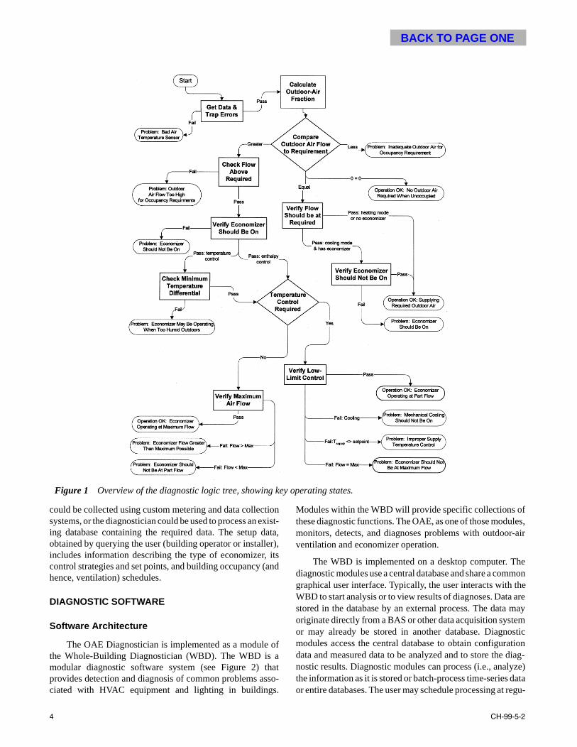
Software Architecture

The OAE Diagnostician is implemented as a module ofthe Whole-Building Diagnostician (WBD). The WBD is amodular diagnostic software system (see Figure 2) thatprovides detection and diagnosis of common problems asso-ciated with HVAC equipment and lighting in buildings.

Modules within the WBD will provide specific collections ofthese diagnostic functions. The OAE, as one of those modules,monitors, detects, and diagnoses problems with outdoor-airventilation and economizer operation.

The WBD is implemented on a desktop computer. Thediagnostic modules use a central database and share a commongraphical user interface. Typically, the user interacts with theWBD to start analysis or to view results of diagnoses. Data arestored in the database by an external process. The data mayoriginate directly from a BAS or other data acquisition systemor may already be stored in another database. Diagnosticmodules access the central database to obtain configurationdata and measured data to be analyzed and to store the diag-nostic results. Diagnostic modules can process (i.e., analyze)the information as it is stored or batch-process time-series dataor entire databases. The user may schedule processing at regu-

Figure 1 Overview of the diagnostic logic tree, showing key operating states.

� &+��

BACK TO PAGE ONE

Diagnostics become highly inaccurate when different ormultiple concurrent faults produce very similar patterns. Inmost cases, faults and their symptoms are nested, i.e., one faultmay have many symptoms and one symptom may be associ-ated with many faults. For example, the occupants report thatthe room temperature is too high. This is a symptom. We caneasily give many possible faults that could cause this symp-tom, such as the thermostat in the room is out of order, or thereheat coil valve in the VAV box is stuck open, or maybe theactuator of the cooling valve doesn’t work anymore. That’s notall. In more complicated situations, several faults may happensimultaneously. Different control loops in the HVAC systemmay be chained together; one could affect another. An abnor-mal control loop could cause faults in other control loops, andthey may finally form a cycle that makes it harder to determinewhich one is the original or the primary source of fault.

The objective of this paper is to apply different methodsand technologies to on-line monitoring of HVAC systemperformance, detection of abnormalities, and diagnosis ofsystem faults. The next sections will present (1) the generationof a three-tier system model based on system components andsystem behavior, (2) the representation of useful knowledgefor real-time system monitoring and FDD, (3) the systemarchitecture and the FDD system model with the implemen-tation schemes used in data collection, data processing, anddata analysis, and (4) results and discussion.

HVAC SYSTEM MODELS

Modeling accuracy is dependent on the depth of knowl-edge captured in the model, the accuracy of the basic structure,the function, and the behavior of objects included in eachclass. Ideally, to build accurate HVAC system models in faultdetection and analysis, information captured from the productdata models used in the design stage of the new system, suchas fan data, ductwork design, shop and as-built drawings, coildesign, and manufacturers’ specification data, are all needed toboth define static attributes and represent the dynamic behav-ior of the entire HVAC system. Furthermore, field measure-

ments and test data defining actual system capacities andsystem response times from the commissioning and applica-tion stages must also go into any useful model.

The information contained in the models must be basedon all of the various sources of knowledge within the HVACindustry, such as

• system design intent and overall mechanical/electricalspecifications as well as all component specifications;

• actual installed components, configurations, and spe-cific equipment engineering data;

• test and balance measurements as well as commission-ing performance data;

• real-time operating data;• actual HVAC system digital controller source code as

well as sequence of operations;• day-to-day maintenance information, i.e., repairs,

replacements, and adjustments both to physical compo-nents, programs, and parameters such as gain, set points,etc.;

• day-to-day input from maintenance and system operat-ing personnel.

To be practical, generic models need to define the under-lying behaviors of a class of similar equipment. As eachsystem configuration may change from building to building,libraries of standardized interoperable models should be madeavailable. These models must be then customizable and adapt-able to various HVAC system types and to each part.

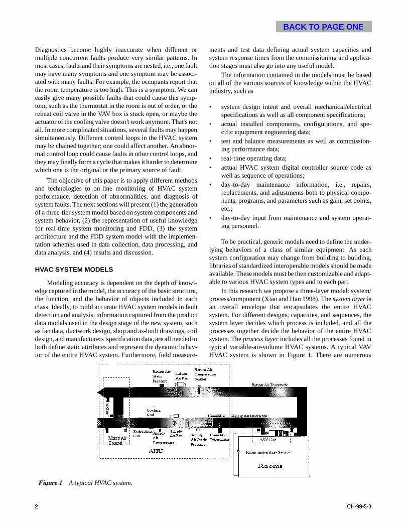
In this research we propose a three-layer model: system/process/component (Xiao and Han 1998). The system layer isan overall envelope that encapsulates the entire HVACsystem. For different designs, capacities, and sequences, thesystem layer decides which process is included, and all theprocesses together decide the behavior of the entire HVACsystem. The process layer includes all the processes found intypical variable-air-volume HVAC systems. A typical VAVHVAC system is shown in Figure 1. There are numerous

Figure 1 A typical HVAC system.

� &+��

BACK TO PAGE ONE

2. Motor control center electricity (2619 complete hourlyrecords)

3. Whole-building thermal energy use (3966 complete hourlyrecords)

4. Whole-building cooling energy use (3964 complete hourlyrecords)

The data set containing these variables has 7944 hourlyrecords in all, but the number of data is less than the numberof hours in the pre-retrofit period because records with one ormore missing variables were omitted from the training data.

Data for the engineering center are available for both thepre-retrofit and post-retrofit periods. However, there are inter-vals of missing data in both periods. In this section, three energyend-uses are considered: whole-building electricity, coolingenergy, and heating energy. Whole-building electricity ismeasured in kWh/h and comprises HVAC electrical energy,lights, equipment, and the supercomputer laboratory. Heatingand cooling energy are measured in units of MMBtu/h. Neuralnetwork models for predicting the use of whole-building elec-tric, heating, and cooling energy were trained on the pre-retrofitdata, and then the results shown in this section were generatedusing the post-retrofit data.

As shown in Table 3, a very dramatic decrease in heatingenergy occurred after the HVAC system was modified. Asubstantial decrease in cooling energy use also occurred.Although the whole-building electrical energy use includessome uses that were not subject to the modification of theHVAC system, the whole-building electrical energy alsodecreased somewhat. The figures noted in Table 3 agreebroadly with corresponding results given by Haberl andThamilseran (1996).

Let us now consider some of the results given by theWBE in a little more detail. Figure 5 shows the computedECI of whole-building electric energy use for the engineer-ing center during 1992. The computed ECI, as defined byEquation 1, is the actual daily energy use divided by the esti-mated daily energy use. Note that over most of the year, thecomputed ECI is in the range 0.6 to 0.9, but toward the endof the year, the ECI increased dramatically. This increasedenergy use is due to severe cold weather, which caused heat-ing pipes to freeze; to compensate, electrical energy wasused for heating instead.

Figure 6 is a detail of Figure 5 showing ECI valuesduring a typical month, September 1992. Note the weeklycycle of values and a general downward trend.

Figure 7 shows the probability of ECI “lower than normal”during September 1992. Note that the increased probabilitiescorrespond to days when the computed ECI was substantiallylower than 0.875, as shown in Figure 6. When the computedECI is only a little lower than 0.875, the probability of “lowerthan normal” ECI decreases. Also see Figure 4.

As a result of this ECI behavior, the WBE generates amessage:

“Daily whole-building electrical energy use is signifi-cantly lower than normal.”

This message is generated on each day of the monthexcept for September 1 through September 3 and September8 through September 10. From Figure 7, it can be seen thatthose are the days on which the probability of ECI “lower thannormal” is relatively small.

Finally, let us consider the total energy savings of theengineering center for the year 1992, as shown in Table 3. Wehave assumed the same energy costs for the engineering centeras Haberl and Thamilseran (1996), namely, $0.0278 per kWhfor electricity, $4.67/MMBtu for cooling energy, and $4.75/MMBtu for heating energy. The “Annual ECI” values listed inthis table are just the total annual actual energy uses divided bythe total estimated energy uses. The heating energy use showsthe greatest reduction, while cooling and whole-building elec-trical use also shows substantial reductions. One wouldsuppose, then, that the HVAC modifications were a success,although the cost of the modifications was not reported.

Figure 5 Computed ECI for whole-building electricenergy use in the engineering center in 1992.The horizontal line at ECI = 0.875 marks theupper limit of “lower than normal” ECI values.See the text for a discussion of the marked peaktoward the end of the year.

Figure 6 Whole-building electric ECI values during themonth of September 1992. Compare this toFigure 7.

4 CH-99-6-2 (RP-811)

BACK TO PAGE ONE

heights for the small-scale experiment are tabulated in Table

2, along with the corresponding full-scale values.

The industrial processes were modeled with 2 ft cubesconstructed from sheet metal, as shown in Figure 4. The cubesize corresponds to 8 ft × 8 ft × 8 ft (2.4 m × 2.4 m × 2.4 m)full-scale processes. The processes were modeled not asspecific industrial processes but as generic processes throughwhich room air was circulated and which released heat andcontaminants. The heat source in the cube was an internal elec-tric heater with a constant velocity fan. The heaters had amaximum power output of 1500 W. The power output was

controlled by variable voltage supplies and was checked bysimultaneous voltage and current measurements.

As shown in Figure 4, each cube had an open slot 1.5 in.high by 1 ft wide located on the bottom of the back side of thecube to serve as an air inlet. Each cube also had an open slot,of the same dimensions, on either side and 2 in. from the topto serve as air and contamination outlets. The contaminationsource was CO2 gas. The CO2 was introduced into the heatedflow using a perforated ping pong ball so that it was wellmixed with the heated flow inside the cube.

Depending on which ventilation configuration was used,one of two industrial process configurations was used: line or

(a)

(b)

(c)

Figure 1 Single wall configuration. (a) Single wallgrille, high-high; (b) single wall grille, low-high; (c) single wall grille, low-low.

(a)

(b)

(c)

Figure 2 Opposite wall configuration. (a) Opposite wallgrille, high-high; (b) opposite wall grille, low-high; (c) opposite wall grille, low-low.

2 CH-99-6-3

BACK TO PAGE ONE

Overhead mixing type systems (see Figure 2) have beenvery popular for the conditioning of office space in NorthAmerica. These systems supply conditioned air to the space bymeans of ceiling-mounted diffusers. These diffusers dischargeair along the ceiling at 55°F to 57°F (13°C to 14°C) and aresized for sufficient outlet velocities to induce room air, mixingthis with the supply air prior to entry into the occupied regionsof the space. Most of the heat transfer between supply androom air occurs above the 6 ft (1.8 m) level. When properlyselected, these outlets produce resultant room velocities in the20 fpm to 30 fpm (0.10 m/s to 0.15 m/s) range throughout theoccupied zone (the lower 6 ft or 1.8 m of the space). Proper

outlet selection results in (1) little or no temperature gradientwithin the occupied zone, (2) return air temperatures (at theceiling) that are similar to that of the room itself, and (3) simi-lar contamination levels throughout the space (and in thereturn airstream) at design conditions.

Underfloor air distribution systems (also illustrated inFigure 2) typically supply air at discharge temperaturesbetween 58°F and 63°F (14°C to 17°C) utilizing special highinduction floor diffusers. This is particularly important assupply air is being introduced within the occupied regions ofthe space, so it is necessary that discharge velocities andtemperatures be significantly reduced before occupants within

Figure 1 Typical underfloor air distribution system.

Figure 2 Overhead and underfloor air distribution systems.

CH-99-6-5 5

BACK TO PAGE ONE

ceiling nozzle type diffuser (cases 1 through 3). In this study,the wall-mounted nozzle type diffuser with an inclined angleof 15°, located at the level of 1.0 m from the floor, has twoopenings with effective areas of 1.29 × 10-3 and 0.32 × 10-3 m2,respectively. The wall-mounted diffuser is assumed to handlea quarter volume of the environmental chamber. For case 7 andcase 8, only the larger opening is used. For case 9, with a highsupply flow rate, both openings are used. In order to under-stand the influence of supply air temperature on airflowperformance and thermal comfort for the ceiling nozzle typediffuser, three cases (case 10, case 11, and case 12) have beentested with 4°C cold air. The sensible heat load and latent heatload is the same as that of case 1, case 2, and case 3.

Part 3—Simulation for a Multi-Cone Circular Diffuser (Case 13 through Case 17)

Detailed studies of a multi-cone circular diffuser are lack-ing in the literature. Recently, Hirano et al. (1997) conducteda very detailed measurement of the airflow and turbulencecharacteristics in the outlet vicinity of a multi-cone circular

diffuser using two sets of crossed hot wire anemometers. Afairly symmetrical airflow pattern was observed. Therefore,Hirano’s experimental data are used to validate the presentairflow model. The geometry of the multi-cone circulardiffuser (with two cones) experimentally studied by Hirano etal. is shown in Figure 2a.

Table 2 summarizes the simulation cases for a multi-conecircular diffuser (with three cones, as shown in Figure 2b).Cases 13 through 15 aim to compare air diffusion character-istics of jets created by the multi-cone circular diffuser undervarious supply flow rates. The objective of case 16 was todetermine the effect of the small hole on the risk of surfacecondensation on the diffuser. The purpose of case 17 was toassess the effect of the cone lip on the performance of air diffu-sion using a multi-cone diffuser.

NUMERICAL METHOD AND BOUNDARY CONDITIONS

For cases 1 through 12, because of the symmetry of theairflow patters in the environmental chamber, only a quartervolume of the room was studied, as shown in Figure 1b. It is

Figure 1 (a) A four-way nozzle type diffuser; (b)volume studied. Unit: mm.

Figure 2a The multi-cone circular diffuser measured byHirano et al. Unit: mm.

Figure 2b The multi-cone circular diffuser studiedin cases 13 through case 1. Unit: mm.

&+��53��

BACK TO PAGE ONE

(6)

where porosity is in percent. Use of the above equationproduces the calculated SHR factors in Table 4.

Now, with a general equation for estimating the SHRfactor, the effect of an architectural screen on rooftop dilutioncan be estimated. First, the stack and screen design parameters

are specified. Second, the SHR is calculated using Equation 6.Next, the height to spread parameter is modified as follows,

, (7)

and is used in the Handbook (ASHRAE 1997) calculations.

TABLE 3 Criteria for Equivalent Stack Height (ESH) Selection

Location of Maximum Concentration

Description

1 If the screen test maximum concentration is located inside the screen, criterion A must be met by any one ESH con-centration inside the screen (not necessarily at the same string distance as the screen test maximum concentration).

Criterion B must be met by all ESH concentrations outside the screen.

2 If the screen test maximum concentration is located outside the screen, criterion A must be met by any ESH concen-tration outside the screen (not necessarily at the same string distance as the screen test maximum concentration).

Criterion B must be met by all ESH concentrations outside the screen.

Criterion C must be met by any ESH concentration inside the screen (not necessarily at the same string distance as the maximum screen test concentration).

Criteria

A The maximum concentration of the ESH must meet or exceed the maximum concentration of the screen test.

B The ESH concentration must be greater than or equal to 80% of the screen test concentration.

C The ESH concentration inside the screen must be greater than or equal to 80% of the maximum screen test concen-tration inside the screen.

Figure 3 Full-scale concentration vs. string distance (µg/m3 per g/s); run 246; 15 ft screen height; 0% screen porosity; 5 ftscreen distance; 10 ft stack height; 5,111 cfm; vertical stack orientation; 16.6 mph wind speed; 0° wind direction.

SHR 0.0081 Porosity×( ) 0.20+=

Y 28.9SHR( )hs

S---------------------

2

=

&+��

BACK TO PAGE ONE

The primary roof support consisted of a series of steeltrusses that form arches spanning the width of the hangar bay,running parallel to the hangar doors. These primary trusses areapproximately 1.0 m (3.3 ft) deep and are spaced 7.4 m (23 ft)on center. The primary trusses are interconnected with a seriesof secondary trusses that are perpendicular to them and run thelength of the hangar bay. The secondary trusses are spaced atintervals ranging from 5.8 m (19 ft) to 6.4 m (21 ft) on center.The metal deck roof is directly attached to a series of steelbeams that sit on top of the primary and secondary trusses.These steel beams are perpendicular to the primary trusses, arespaced 1.5 m (5 ft) to 2.1 m (7 ft) on center, and vary in heightfrom 0.2 m (8 in) to 0.3 m (12 in).

The roof was insulated via a barrel-shaped suspended tileceiling that was supported by a conventional suspended tileceiling grid located at the same elevation as the bottom of thesteel beams. The ceiling tiles were removed in the middle bayand the adjacent bays prior to testing.

Experimental east and west were designated to be thedirections parallel to the 13.4 m (44.0 ft) draft curtain andpointed along the direction of the barrel roof. Experimentalnorth and south directions ran perpendicular to the draftcurtain. Thermocouples located 0.31 m (1.0 ft) beneath theceiling were at radial distances from the fire center of 3.0 m(10 ft), 4.6 m (15 ft), 6.1 m (20 ft), and 6.7 m (22 ft) in the southdirection and 3.0 m (10 ft) and 6.1 m (20 ft) in the north direc-tion. Thermocouples located 0.31 m (1.0 ft) beneath the ceil-ing were at radial distances from the fire center of 3.0 m (10ft), 6.1 m (20 ft), 9.1 m (30 ft), 12.2 m (40 ft), 15.2 m (50 ft),and 18.3 m (60 ft). Additional thermocouples were positionedat many of these locations and are represented in Figure 3.

TABLE 4 Test Summary for Fire Sizes Larger than 3 MW (2800 Btu/s) for the 22 m (73 ft) Facility*

Test NumberPan Size

m (ft)

Fire Size(1 ± 10%)

MW (Btu/s)Fuel Type

Sprinkler Act. † s(Wet Pipe)

(QR 79°C)(175°F)

Smoke Det.Act.†s(P.B.‡/S.P.** )

± 10 s

14 2.5 (8.2) Dia 7.9 (7500) JP-5 361.±10. 38/65.

15 3.0 × 3.0 (10 × 10) 15.7 (14900) JP-5 119.±10. 33/46.

16‡‡ 2.5 (8.2) Dia 7.0 (6600) JP-5 No T††/51.

17 3.0 × 3.0 (10 × 10) 14.3 (13600 JP-8 100.±10. 27/30.

18 2.0 (6.6) Dia 4.9 (4600) JP-5 No 42/49.

19‡‡ 2.5 (8.2) Dia 9.1 (8600) JP-5 No 39/56.

20 3.0 × 3.0 (10 × 10) 14.6 (13800) JP-5 101.±10. 31/38.

21 4.6 × 4.6 (15 × 15) 33 (31000) JP-5 87.±10. 30/37.

* The sprinklers were located 3.1 m (10 ft) from plume center.† Activation times represent the first time that a detector activated at that distance from the fire. Activation times for detectors should include a ±10 s uncertainty in establishingthe start time of the experiment.‡ Denotes a projected beam detector with the beam located 1.3 m (4.3 ft) below the ceiling and passing through plume center.** Denotes a single-point smoke detector located 3.1 m (10 ft) from plume center.†† Trouble signal.‡‡ Open door test.

Figure 2 Plan view of 22 m (73 ft) hangar.

&+��

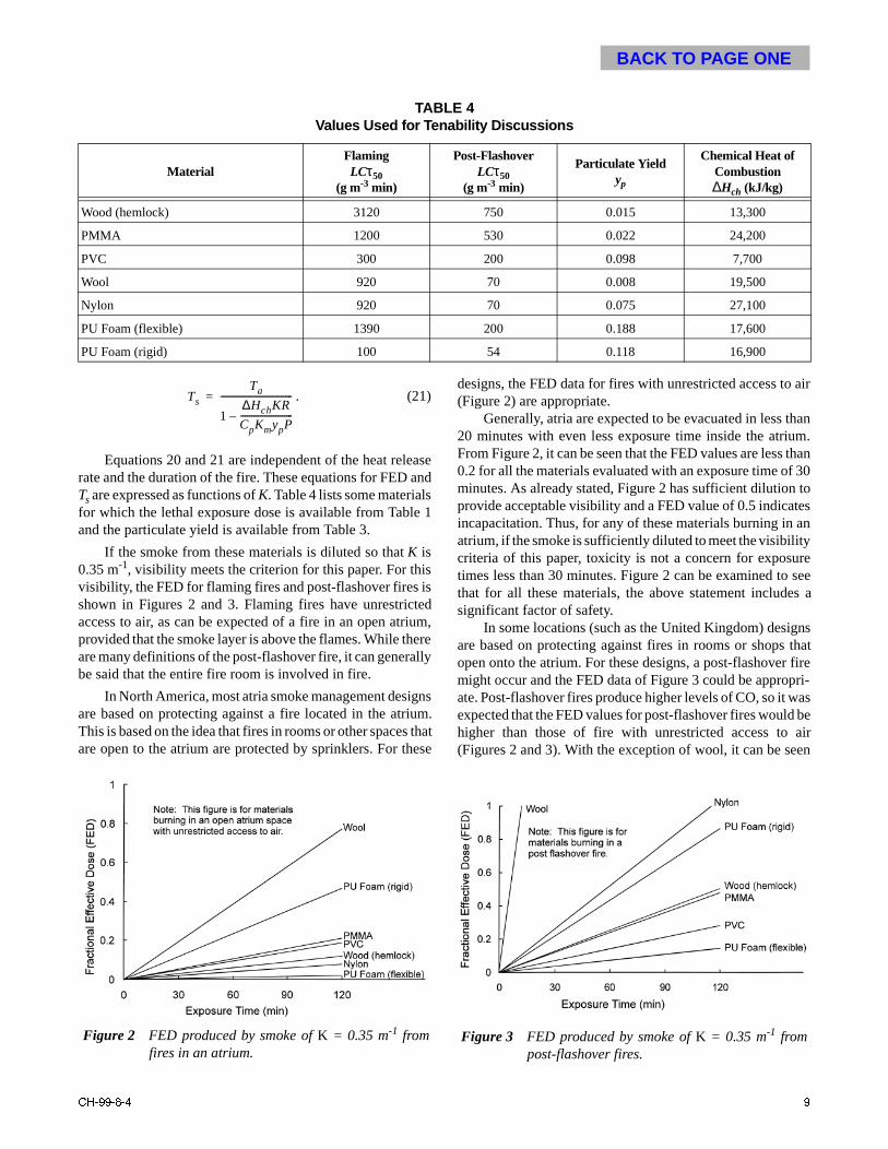
BACK TO PAGE ONE

. (21)

Equations 20 and 21 are independent of the heat releaserate and the duration of the fire. These equations for FED andTs are expressed as functions of K. Table 4 lists some materialsfor which the lethal exposure dose is available from Table 1and the particulate yield is available from Table 3.

If the smoke from these materials is diluted so that K is0.35 m-1, visibility meets the criterion for this paper. For thisvisibility, the FED for flaming fires and post-flashover fires isshown in Figures 2 and 3. Flaming fires have unrestrictedaccess to air, as can be expected of a fire in an open atrium,provided that the smoke layer is above the flames. While thereare many definitions of the post-flashover fire, it can generallybe said that the entire fire room is involved in fire.

In North America, most atria smoke management designsare based on protecting against a fire located in the atrium.This is based on the idea that fires in rooms or other spaces thatare open to the atrium are protected by sprinklers. For these

designs, the FED data for fires with unrestricted access to air(Figure 2) are appropriate.

Generally, atria are expected to be evacuated in less than20 minutes with even less exposure time inside the atrium.From Figure 2, it can be seen that the FED values are less than0.2 for all the materials evaluated with an exposure time of 30minutes. As already stated, Figure 2 has sufficient dilution toprovide acceptable visibility and a FED value of 0.5 indicatesincapacitation. Thus, for any of these materials burning in anatrium, if the smoke is sufficiently diluted to meet the visibilitycriteria of this paper, toxicity is not a concern for exposuretimes less than 30 minutes. Figure 2 can be examined to seethat for all these materials, the above statement includes asignificant factor of safety.

In some locations (such as the United Kingdom) designsare based on protecting against fires in rooms or shops thatopen onto the atrium. For these designs, a post-flashover firemight occur and the FED data of Figure 3 could be appropri-ate. Post-flashover fires produce higher levels of CO, so it wasexpected that the FED values for post-flashover fires would behigher than those of fire with unrestricted access to air(Figures 2 and 3). With the exception of wool, it can be seen

TABLE 4 Values Used for Tenability Discussions

MaterialFlamingLCτ50

(g m-3 min)

Post-FlashoverLCτ50

(g m-3 min)

Particulate Yieldyp

Chemical Heat of Combustion∆Hch (kJ/kg)

Wood (hemlock) 3120 750 0.015 13,300

PMMA 1200 530 0.022 24,200

PVC 300 200 0.098 7,700

Wool 920 70 0.008 19,500

Nylon 920 70 0.075 27,100

PU Foam (flexible) 1390 200 0.188 17,600

PU Foam (rigid) 100 54 0.118 16,900

Ts

Ta

1∆HchKR

CpKmypP------------------------–

---------------------------------=

Figure 2 FED produced by smoke of K = 0.35 m-1 fromfires in an atrium.

Figure 3 FED produced by smoke of K = 0.35 m-1 frompost-flashover fires.


buildings chosen also meet the site selection criteria, includingtwo sites from each of three size ranges: small—less than 45apartments; medium—45 to 80 apartments; large—greaterthan 80 apartments.

The project research buildings are characteristic of theolder and predominant stock of the over 120,000 New YorkCity multi-family buildings. Table 1 lists the sites and theirsize (in number of apartments).

The buildings ranged in size from 25 to 103 apartments ineither five or six above-ground stories. All but one havecombination steam and DHW-generating steel tube boilers.One site has a combination system with a cast iron boiler.DHW is generated by a “tankless coil” located under thesurface of the boiler water.

All six buildings in this study had a forced recirculationsystem with the pump running continuously. Figures 1 and 2depict representative DHW consumption and recirculationflow patterns found in the buildings.

Control Strategies

Data from a prior DHW modeling project (Goldner andPrice 1996) suggested that it may not be necessary to contin-uously operate forced DHW recirculation systems in multi-

family buildings, as is the practice in most buildings. Therecirculation control research project detailed here measuredthe energy savings that can be realized by cycling these pumpsusing a base case of continuous operation and three other oper-ating strategies:

a. Base case (continuous operation): Strategy A is used as abase case against which to determine the savings achievableby the other approaches.

b. Shutdown during the overnight period: Strategy B’sapproach is to attempt to save energy by shutting down thepumps at night when few, if any, people are using hot water.After careful review of the data, it was determined that thepumps should be shut off from 11:50 p.m. to 5:20 a.m. eachnight.

c. Shutdown during the peak morning and evening periods:Strategy C’s approach is to attempt to save energy by shut-ting down the pumps during the peak DHW usage periods,when the large volume of usage is, in and of itself, causingcirculation to occur. Data review determined that the pumpsshould be shut off from 5:45 a.m. to 8:15 a.m. each morningand 5:45 p.m. to 9:15 p.m. each evening.

d. Cycling by a return line aquastat: Strategy D evaluatesrunning the pump only when the DHW temperature in thebasement return line falls below 110°F (61.1°C), ascontrolled by a return line aquastat.

PROJECT METHODOLOGY

Realizing that different buildings use varying volumes ofDHW, it was essential that this research compare the effects ofoperating the DHW recirculation systems with each strategy ateach of the six selected sites. These buildings were selectedand equipped with the necessary pump control devices (botha return line mounted aquastat and a programmable timeclock,each wired into the recirculation pump) and monitoring equip-ment. This research project was designed to isolate those

TABLE 1 Project Buildings

ID# Address Apartments

12 Beach St. 25

31 Tinton Ave. 42

7 Burr Ave. 60

9 Buhre Ave. 80

10 Trinity Ave. 102

30 St. Theresa Ave. 103

Figure 1 DHW consumption and recirculation flowsfor Building 7, weekday.

Figure 2 DHW consumption and recirculation flowsfor Building 7, weekend.


Figure 2 Table 1 as it appears in the 1995 ASHRAE Handbook—HVAC Applications.


device is tested separately, more reliable reference data areavailable for fault detection and diagnosis (FDD). The instal-lation and commissioning phases should be performed basedon specific plans made for these tasks. During operation andmaintenance, the most essential parts of the system should bemonitored and controlled. From each life-cycle phase, feed-back is obtained that can be used in developing second-gener-ation products and also during operation and maintenance ofexisting equipment.

This paper describes the process of how the performancefactors for one brand of commercial AHU are established,how the performance requirements are defined based on theseperformance factors, and how these criteria can be connectedto practical FDD methods in different life-cycle phases. Inaddition, this paper suggests several methods that can be usedfor performance monitoring. Examples of the implementationof the most promising methods are also given.

Figure 2 shows a schematic diagram of one possibleAHU. The system considered includes fans andAHU components for

• air filtering,• heating,• heat recovery,• indirect humidification (if required),• cooling (if required), and• air mixing.

The system is called a “building service unit”and it uses variable air volume. The heart of thebuilding service unit is the liquid circulated heatrecovery unit, which is used for both heating andcooling. Extra cooling capacity is available throughindirect humidification (humidifier in the returnairstream) and from the heat transfer network. Vari-ous heat sources are available. Often the heatingcapacity of the exhaust air and waste heat from

refrigerators (condensing water) are the primary heat sources.District heating is also frequently used as a heat source.

LINKING PERFORMANCE FACTORS TO FAULT DETECTION AND DIAGNOSIS

Figure 3 illustrates how performance factors areconnected to fault detection. The boxes in the figure representthe process from defining performance factors to the detectionof faults. Under the boxes there are examples of possiblecontents of each box. For example, indoor climate, energyconsumption, maintenance costs, and system reliability areperformance factors for air-conditioning systems. When aparticular system is considered, certain criteria for thesefactors can be given or specified, e.g., supply air temperatureset points, outdoor air requirements, and air purity criteria.The criteria can be based on building codes, design require-ments, and/or user requirements. Matsunawa et al. (1996)discussed the cost/benefit analysis of a building optimization

Figure 2 A schematic diagram of one possible air-handling unit. The supply air side is drawn on upper side.

Figure 3 Connection of performance factors to fault detection.


The control wires for each of the ballasts used at thedemonstration restaurant were terminated with a standardRJ11 telephone style connector that allowed for a simple plug-and-play interconnection of the ballasts with each other andwith the photosensors (Figures 3 and 4). Other control devices,such as dimmers, could also be added to this system. In addi-tion, this system used a single photosensor to control lightingfixtures on different electrical circuits, making zoning andrezoning a simple task.

These innovations dramatically reduced the initial costfor this system, bringing the installed cost in line with the stan-dard, noncontrollable systems. At the demonstration restau-rant, the system saved over 7,000 kWh/yr (25.2 GJ/yr) in theplay area and dining areas (PG&E 1996-97), resulting in apayback of less than one year. Although ideal for new

construction, controllable ballasts can also be consideredduring a retrofit of an existing restaurant. Figure 5 shows atypical dimming load profile in response to available daylight.

LIGHT PIPES

Light pipes are tubular skylights that bring daylight intoa restaurant. They are particularly effective in windowlessspaces, such as restrooms, kitchens, and storerooms, but canalso be used to brighten up darker areas of a dining room orimprove the lighting quality at a service counter. Light pipesare unique because they can be used in applications where afull-sized skylight could not be used for reasons of availablespace or security. Also, the reflective pipes can be installed atan angle between the roof and the interior ceiling and thedistance between the roof and ceiling can vary greatly withoutappreciable degradation of the light delivered at the diffuserdome.

Light pipes save energy when used in combination withelectronic controllable ballasts by increasing the amount ofavailable daylighting within the restaurant. The light pipesinstalled at the demonstration restaurant were 13 in. in diam-eter. Four of the six light pipes used in the demonstrationrestaurant were applied in areas that already had sufficientdaylighting, so their contribution to energy savings wassecondary to their aesthetic value. In a follow-up applicationat another restaurant, the experience gained at the demonstra-tion restaurant was used to better locate the light pipes inseveral windowless spaces, including the kitchen, storerooms, and restrooms, where they had more effect on the elec-tronic controllable ballasts. A sectional view of a light pipe isshown in Figure 6.

LOW-TEMPERATURE OCCUPANCY SENSORS

The lighting in walk-in coolers and freezers is typicallyleft on all the time because of inconvenience and lack of incen-tive for manual switch control. There may be anywhere fromone to six fixtures in a standard QSR walk-in, which are typi-cally lamped with 75 W incandescent bulbs. Low-temperatureoccupancy sensors save energy by automatically turning thelights off in the walk-in cooler and freezer when they are unoc-cupied.

At the demonstration restaurant, the low-temperatureoccupancy sensors paid for themselves in less than a year,saving 3,265 kWh/yr (11.75 GJ/yr)—an 80% reduction inenergy use (PG&E 1996-97). One sensor controlled the twofixtures in the walk-in cooler, and a second sensor controlledthe four fixtures in the freezer. Additional savings wereachieved by reducing the heat load on the refrigeration

TABLE 1 Energy Savings Estimated by Each of the Three Analysis Techniques

Technique Control Comparison DOE2 ModelMonitoring Results

(Including Lot Lights)Monitoring Results

(Excluding Lot Lights)Overall Estimate

Estimated Savings 18% 9% 18% 14% 12%-18%

Figure 3 Easily installed controllable ballast system.

Figure 4 Standard RJ11 connector used on ballast controlwiring.


Weather

Figure 2 shows the differences between the monthly aver-age dry-bulb temperature for the Antioch weather file and theBay Point weather file. In general, Bay Point was severaldegrees warmer during the winter and swing seasonscompared to the Antioch WYEC2 weather. This may be due,in part, to the location of the Bay Point weather instrumenta-tion, which was on the roof of the store. The store and itssurrounding parking lot may serve as a heat “island” thatcauses elevation of the ambient temperatures. It may also betrue that the conditions in Bay Point were usually warmer inthe winter and swing seasons than in Antioch. From a model-ing viewpoint, this is an area that deserves additional research.

Figure 3 shows the differences in monthly averagehumidity ratios for two weather files. Moisture conditionswere reasonably similar during the year, except during latefall/early winter.

Lighting

The interior lighting systems in the baseline restaurantand the EEM restaurant used fluorescent T-8 lamps with elec-

tronic ballasts. The electric lighting system in the EEM designwas enhanced with two energy efficiency measures:

• Daylight harvesting using dimming ballasts with day-light sensors in two zones in the dining room, therestrooms, and two zones in the play area.

• Six tubular skylight fixtures, also called “light pipes,”two over the customer order counter, two in the playarea, and one each in the two customer restrooms.

For daylight harvesting control, the dining zone was splitinto two parts, one toward the front windows and one towardthe interior space close to the restrooms. The dining zone hadtwo light sensors that permitted the electronic dimmingballasts in each zone to reduce power if sufficient daylight wasavailable. The play area was also divided into two parts, eachcontrolled by separate daylight sensors. Daylight harvesting ineach restroom was dependent on the presence of a light pipe.Each restroom had a fiber-optic light sensor that permitted onefixture adjacent to the wash basins to operate at reduced powerif sufficient light was available from the light pipe.

Daylight harvesting was modeled as an independentmeasure, but the light pipes were modeled assuming thedaylight harvesting measure was in use. The light pipesconsisted of vertical tubes that penetrated the roof and termi-nated below the ceiling tile with a translucent hemisphericaldiffuser. Sunlight, or available daylight on cloudy days, wastransmitted through the light pipe, providing better qualitylight and reducing the amount of electric lighting needed in theimmediate vicinity.

Table 5 shows the connected lighting power in each ofthe interior zones. The lighting circuits in the building werecontrolled by an energy management system through whichthe restaurant management could set on/off times by day ofthe week. The exterior accent lighting on the building totaled1.9 kW. The parking lot lights totaled 15.0 kW in the initialmodel and were controlled by a photosensor, which turnedthem on when light levels fell below a predetermined level,and a timer, which turned them off after business hours. Inthe model, the exterior accent lighting and the parking lotlighting were scheduled according to weekday and weekendoperating times, as well as seasonal changes in availablesunlight (in the morning and the evening).

Model Calibration and Validation Changes for Light-ing. Measured data showed that the aggregated, interior light-

Figure 2 Comparison of Antioch and Bay Point dry-bulbtemperature.

Figure 3 Comparison of Antioch and Bay Point humidityratio.

TABLE 5 Lighting Power by Zone

ZoneLighting Power

(w/ft2)Lighting Power

(w/m2)

Kitchen 0.97 10.4

Dining (including restrooms) 1.28 13.8

Play area 1.08 11.6


hood. For the demonstration restaurant with a two-speedsystem over the “clamshell” griddles, the high-speed exhaustrate was 1255 cfm (592 L/s) vs. the applicable code value of1950 cfm (920 L/s). The two-speed exhaust fan also savesenergy by turning down the exhaust when the clamshell grid-dle is in standby mode. Since this griddle is primarily used forbatch cooking, there are significant amounts of time when it isin a standby or idle mode (Spata and Turgeon 1995). Underlow-speed operation, the exhaust rate was 630 cfm (297 L/s).Table 1 compares the exhaust ventilation rate scenarios usedfor this QSR cost-saving comparison.

The energy consumption for scenarios 1 and 2 were calcu-lated using the OALC for outdoor airflow rates that matchedthe exhaust rates shown in Table 1. For scenario 3, one initiallywould think that precise knowledge of the schedule would benecessary. Figure 4 plots the power input of the two-speedexhaust fan over a typical day. The 0.25 kW line representsoperation at low speed, and the 0.45 kW data points representoperation at high speed. The data points in between are causedthrough time averaging, when the system was operating athigh speed and low speed during part of the same measure-ment cycle. The plot shows rather random high and low peri-ods throughout the day. Averaging the daily fan power profilefor a month shows that the high/low profile turns into a ratherstable line at 75% of maximum fan power input. Knowledgeof power input and flow for high- and low-speed settings

allows calculation of an effective flow rate at 75% of fanpower as follows:

The effective power (= average power) is 75% of maxi-mum input:

Peff = 0.75 ⋅ 0.45 kW = 0.3375 kW.

The average fan power is the fraction of time on lowmultiplied by the low power input plus the fraction of timewith the fan on high times the power consumption on high.

Peff = tlow ⋅ 0.25 kW + thigh * 0.45 kW.

Since the total of time on low fraction and time on highfraction needs to be one (tlow + thigh = 1), the previous equationcan be rewritten as

Peff = tlow ⋅ 0.25 kW + (1 − tlow) ⋅ 0.45 kW.

The result of this equation istlow = 56%,thigh = 44%.

So we can calculate an effective flow rate:

Floweff = 0.56 ⋅ Flowlow + 0.44 ⋅ Flowhigh.

With the low flow rate being 630 cfm (297 L/s) and thehigh flow rate being 1255 cfm (592 L/s), the effective flow ratebecomes 905 cfm (427 L/s). This effective flow rate alloweduse of the OACL.

Energy Savings Estimates for the Optimized Two-Speed Exhaust System

This example is based on a demonstration quick servicerestaurant in Bay Point, California, and a second QSR inChicago, Illinois.To reflect locations in the U.S. with a signif-icant heating load, the OALC calculation example ispresented for the Chicago site (Figure 5). The QSR kitchenhad two 3-ft griddles and a four-bank fryer station. Since thedemonstration restaurant only had two-speed ventilation forthe griddle, this paper only presents the savings potential ofthe griddle exhaust system. The total ventilation savingspotential for the QSR is, of course, higher than reported inthis paper since the fryer-hood system was also operatedbelow the code rate. It also would be feasible to design thefryer hood to operate under a two-speed scenario.

TABLE 1 Backshelf Hood Exhaust Rates

Appliance→ “Clamshell” Griddle

Vent Speed ↓ \ Op. Condition → Idle/Standby Cooking

1) Code flow rate: 1950 cfm (920 L/s)

1950 cfm(920 L/s)

2) Custom hood flow rate: 1255 cfm (592 L/s)

1255 cfm (592 L/s)

3) Custom hood two-speed: 630 cfm (297 L/s)

1255 cfm (592 L/s)

Figure 4 Measured daily energy consumption profile forthe two-speed exhaust fan.


ABSTRACT

This paper describes the application of evaporative cool-ing strategies to the kitchen HVAC outdoor air intake, diningarea HVAC condensers, and to the total cooling of a large,separate play area in a quick service restaurant (QSR). Thepaper includes a discussion of the types of evaporative coolersused, including media and once-through water flow, as well asthe benefits and shortcomings of evaporative cooling in a quickservice restaurant application. Measured data were used todetermine the performance of the systems and to developmodels used to predict cooling season performance. Theperformance of all evaporative cooling strategies reducedenergy consumption, but they all required adjustments andmodifications during the evaluation period. Proper commis-sioning after installation would have ensured peak perfor-mance sooner.

INTRODUCTION

A large quick service restaurant (QSR) operation formedan advisory panel of energy efficiency and environmentalexperts to assist in creating an energy-efficient QSR concept.The QSR management planned to incorporate the energy effi-ciency concepts in four restaurants in different climatic zones.In cooperation with the QSR design and construction team, aCalifornia utility provided design and construction support foran energy-efficient QSR in Bay Point, California (PG&E1998). Three different evaporative cooling technologies wereinstalled in this restaurant to evaluate their performance andcost-effectiveness. The results were used to assist quickservice restaurant designers and management in determiningif these technologies should be included as a standard speci-fication item in new stores or as an option and to determine if

the technology is a cost-effective application in a retrofit situ-ation.

Design Considerations

Although many evaporative cooling systems recirculatethe water passing through the evaporative media using a sump,in this application all the evaporative cooling systems used aone-pass system with no recirculation. Controlling the waterflow to the media is more important in a one-pass system tominimize the amount of water going down the drain. Theinitial setup of the water flow controls is critical, as it affectsthe water consumption and thermal performance of thesystem. The advantages of a one-pass system are lower main-tenance costs and the elimination of a standing water sump,which is a potential health risk if maintenance is neglected. Apotential disadvantage is higher water and sewage cost.

Evaporative Cooling Technologies

Three different evaporative cooling technologies wereinstalled, including a direct evaporative cooler serving theplay area, a direct evaporative precooler on the outdoor airintake of the kitchen HVAC unit, and add-on evaporativeprecoolers on the dining HVAC unit condensers. Descriptionsof these technologies follow.

Kitchen Outdoor Air Evaporative Precooler. The 10ton HVAC unit specified to serve the kitchen was retrofittedwith an evaporative precooler on the makeup air inlet. Thepurpose of the evaporative precooler was to reduce thetemperature of the air entering the unit, thus reducing theamount of mechanical cooling required to maintain accept-able conditions in the kitchen. The evaporative precoolerconsists of evaporative cooler media that cools the incoming

The Application of Three Different Evaporative Cooling Strategies to a Quick Service Restaurant

Stuart S. Waterbury, P.E. Tor E. Allen Richard Young

Stuart S. Waterbury is a senior engineer at Architectural Energy Corporation, Boulder, Colo. Tor E. Allen is a research engineer at PG&EPacific Energy Center, San Francisco, Calif. Richard Young is lead engineer at PG&E Food Service Technology Center, San Ramon, Calif.

CH-99-20-4


A water-to-refrigerant counterflow heat exchanger wasinstalled in this facility, as shown in Figure 2. In one shell, fourrefrigerant tubes were installed in parallel. The refrigerantmass flow rates within each tube are assumed to be the same.The heat exchangers were installed horizontally. The specifi-cations for the evaporator and gas cooler are shown in Table 1.

Positive displacement compressor prototypes weredesigned and built, as shown in Figure 3. The design capacityof the prototypes was 11 kW. The original prototype, ahermetic compressor, was modified to have a removable lid toenable repairs and investigation of inner parts. More detaileddesign aspects can be found in Hwang and Radermacher(1998).

Instrumentation and Data Acquisition

Instrumentation and a data acquisition system wereinstalled in the CO2 test facility. CO2 and water temperaturesand pressures were measured at the locations indicated inFigure 1. Refrigerant mass flow rate, water volume flow rates,and compressor power input were also measured. Softwareroutines to collect and analyze the data were developed. CO2refrigeration cycle performance was evaluated in terms ofevaporator water-chilling capacity and coefficient of perfor-mance (COP). The water-side capacity and refrigerant-side

capacity were evaluated and compared in each test to verifytest results.

Testing of Experimental Setup

Two steps were taken to verify the test facility’s perfor-mance measurements. First, the water-side capacity measure-ment was verified with a 2 kW heater. The average error of thewater-side capacity measurement relative to the heater powerwas less than 0.3%. Second, the refrigerant-side capacity andenergy balance measurement were verified with conventionalcompressors. Two compressors for R-22 with 7 kW and 18 kWcapacity were utilized for this purpose. The energy balanceerrors were within 4%, which is within the range of acceptableuncertainty for the experiment.

TEST RESULTS

Preliminary Charge Optimization with Prototype CO2 Compressor

The prototype CO2 compressor was tested with a coun-terflow heat exchanger. The results of the preliminary chargeoptimization tests are shown in Figure 4. In these tests, themetering valve opening was adjusted to vary the gas coolingpressure. The figure indicates that the 3.5 kg and 4.0 kgcharges demonstrated higher performance than that shown bythe 3.0 kg charge. The optimum charge was determined to be

Figure 2 Counterflow heat exchanger.

Figure 3 CO2 compressor prototype.

TABLE 1 Specifications of Heat Exchangers

Heat Exchanger Evaporator Gas Cooler

Shell Dimension (cm) ID: 2.54 × t 0.165 × 600(1 in. × 0.065 in. × 19.7 ft)

ID: 3.18 × t 0.165 × 600(1.25 in. × 0.065 in. × 19.7 ft)

Tube Number of Tubes (ea)Dimension (cm)

4OD: 0.952 × t 0.165 × 600

(0.375 in. × 0.065 in. × 19.7 ft)

4OD: 0.952 × t 0.165 × 600

(0.375 in. × 0.065 in. × 19.7 ft)


the “reheat to cool” column represent extra heating require-ments due to centrally cooling the supply air. The central cool-ing may occur when the economizer operates and does notnecessarily translate to a chiller load.

The “system cool” column separates the cooling coil loadinto latent and sensible components. The column also presentsthe cooling accomplished by the economizer. This quantity isthe outdoor airflow rate multiplied by the enthalpy differencebetween the outdoor air and return air when the economizer isoperating. Its large column segment shows the significantcontributions to cooling a properly working economizer canhave.

Some important observations about system performancecan be made from Figure 1. The annual fan energy use of theVAV system is about 40% of the CAV system. The fan savingsdetermined by the simulation is consistent with measuredvalues reported for VAV retrofits of CAV systems (Jagemar1994). Reheating cool air makes up most of the system load onthe boiler for the CAV system. The “reheat to heat” systemload is much greater than the heat load due to thermal mixing.As expected, the “reheat to cool” energy is much reduced inthe VAV systems. The significantly higher CAV system loadsshow the disadvantage of system designs based on noncoin-cident loads and constant airflow rate. The VAV system canrespond more dynamically to loads.

The CAV to VAV retrofit not only reduces fan energyconsumption but also significantly reduces cooling and heat-ing energy use. This results from the interdependence ofsystem cooling loads and heating loads on each other and onairflow rate. Additionally, the VAV retrofit substantiallyreduces system and plant equipment size requirements. Forthe location analyzed, the peak reheat load for the VAV systemis about 75% of the CAV system load. The peak cooling coilload for the VAV system is about 65% of the CAV system load.

Improving System Design Using the Second Law

The low ratio of energy produced (building load) toenergy consumed (plant energy) for heating in Figure 1demands attention. While the VAV design is an improvementover the CAV, the first law efficiency for providing spaceconditioning to the building is still low. Insights for improvingsystem performance through design and operational changescan be gained by considering the second law. Second law guid-ance aids in the detection and avoidance of unnecessary deple-tion of useful work in a process. Second law guidelines that areparticularly relevant to HVAC distribution systems include(Sama 1995) the following:

1. Minimize the mixing of streams with different tempera-tures and pressures.

2. Do not discard heat at high temperatures to the ambient orto cooling water.

3. Do not heat refrigerated streams with hot streams.

4. Heat (or refrigeration) is more valuable the further thetemperature is from ambient.

5. The larger the mass flow, the larger the opportunity to save(or waste) exergy.

Most of these considerations are common sense. Yet, inthe design and operation of the CAV and VAV reheat systems,they are not adhered to. While there are many criteria otherthan thermodynamic performance for developing an accept-able design, any opportunities for reducing the depletion ofuseful work should be recognized when making design deci-sions.

The improvement of VAV performance to CAV can beexplained by second law considerations. Airflow rates arelower for the VAV system, which reduces other second lawerrors including reheating cool air, discarding warm return air,and mixing streams at different temperatures. In addition, fan

Figure 2 Useful work depleted by VAV system during one hour.


room sensible heat ratio of 0.95, an economic life-cycleof 15 years, and an annual interest rate of 7.5%. It is rec-ognized that wet coils have shorter lives than dry coils.

• Excluded from the analysis are the costs for cleaningcoils in terms of whether they are dry or wet and thenumber of rows, filter replacements, and maintainingintegrity of pipework insulation and vapor barriers.

Figure 1 indicates the specific exergy cost throughout theprocess from the chiller plant to the final product of buildingcooling, of the base system optimized as described previously.Two figures are given for each stage, whereby the cost flowsare numbered 1 to 6, the cbz figures that indicate the cost,taking into account the exergy and plant costs, whereas the cb

figures indicate these costs in terms of the exergy costs alone.The term z refers to capital costs, w to electric power and plantdenominations. Zqr indicates the specific capital costs associ-ated with the overall cooling system, and it is variable. Pleaserefer to the nomenclature section, including subscripts andsuperscripts.

The analysis tool used was to determine the exergy costs,and exergy and capital costs and their relative cost increase,between the exergy flow (indicated in Figure 1) into and outof each plant, as indicated separately in Table 1. A carefulanalysis of these costs (last two columns in Table 1) indicatesthat the cost of chilled water has the highest increase, withrespect to its incoming value, between cost flows 1 and 2. Thenext highest ratio is for the fan coil units between flows 4 and5. In order to improve the overall system efficiency, an appro-priate assessment of real achievable economic and exergyfactors must be considered.

Based on the increase of costs, the independent systemvariables were selected for minimization of life-cycle costs.However, in terms of quality for people, the most importantvariable is the air OFF coil temperature, which has the potentialto cause cold drafts. Therefore, the life-cycle costs were indi-vidually optimized by minimizing the objective function fordifferent values of air OFF coil temperatures. To optimize thefan coil system design, the independent design variablesselected were the leaving chilled water temperature, chilledwater temperature difference, pipework friction loss, roomrelative humidity, number of coil rows, and number of fan coilunits

• The optimization of the chiller had been limited byparameters imposed by the manufacturer. The manufac-

Figure 1 Diagram of base design.

TABLE 1 Base Design Exergy and Flow Costs

Cost Flow (Figure 1)

Exergy, kW (b)

Exergy Cost, £/kWh (cb)

Exergy and Capital Cost, £/kWh (cbz)

1 58.7 0.05 0.05

2 8.46 0.36 1.06

3 8.46 0.36 1.18

4 8.25 0.37 2.65

5 3.65 0.94 10.42

6 0 N/a N/aNote: £1 is approximately 1.6 $U.S.

errata ashrae transactions, vol. 105, part 1 several papers in the transactions …...

Documents