Error analysis of projection methods for non inf-supstable mixed finite elements. The transient Stokes

problem.

Javier de Frutos∗ Bosco Garcıa-Archilla† Julia Novo‡

Abstract

A modified Chorin-Teman (Euler non-incremental) projection method and amodified Euler incremental projection method for non inf-sup stable mixed finiteelements are analyzed. The analysis of the classical Euler non-incremental andEuler incremental methods are obtained as a particular case. We first prove thatthe modified Euler non-incremental scheme has an inherent stabilization that allowsthe use of non inf-sup stable mixed finite elements without any kind of extra addedstabilization. We show that it is also true in the case of the classical Chorin-Temammethod. For the second scheme, we study a stabilization that allows the use ofequal-order pairs of finite elements. The relation of the methods with the so calledpressure stabilized Petrov Galerkin method (PSPG) is established. The influence ofthe chosen initial approximations in the computed approximations to the pressureis analyzed. Numerical tests confirm the theoretical results.

keywords Projection methods, PSPG stabilization, non inf-sup stable elements

1 Introduction

In this paper we analyze a modified Chorin-Temman (Euler non-incremental) projectionmethod for non inf-sup stable mixed finite elements. The analysis of the classical Eulernon-incremental method is obtained as a particular case. We prove that both the modifiedand the standard Euler non-incremental schemes have an inherent stabilization that allowsthe use of non inf-sup stable mixed finite elements without any kind of extra added

∗Instituto de Investigacion en Matematicas (IMUVA), Universidad de Valladolid, Spain. Researchsupported by Spanish MINECO under grants MTM2013-42538-P and MTM2016-78995-P (AEI/FEDER,UE) (frutos@mac.uva.es)†Departamento de Matematica Aplicada II, Universidad de Sevilla, Sevilla, Spain. Research supported

by Spanish MINECO under grant MTM2015-65608-P (bosco@esi.us.es)‡Departamento de Matematicas, Universidad Autonoma de Madrid, Instituto de Ciencias Matematicas

CSIC-UAM-UC3M-UCM, Spain. Research supported by Spanish MINECO under grants MTM2013-42538-P and MTM2016-78995-P (AEI/FEDER, UE) (julia.novo@uam.es)

1

arX

iv:1

611.

0451

0v2

[m

ath.

NA

] 2

8 Fe

b 20

17

stabilization. Although this result is known (see for example [10]) to our knowledgethere are no proved error bounds for the Chorin-Temam method with non inf-sup stableelements in the literature (see below for related results in [1]). For the closely-relatedEuler incremental scheme we analyze a modified method for non inf-sup stable pairs offinite elements. In this case an added stabilization is required. The analysis of a stabilizedEuler incremental scheme is also obtained as a consequence of the analysis of the modifiedmethod. We establish the relation of the methods with the so called pressure stabilizedPetrov Galerkin method (PSPG).

It has been observed in the literature that the standard Euler non-incremental schemeprovides computed pressures that behave unstably for ∆t small and fixed h if non inf-supstable elements are used, see [3]. With our error analysis we clarify this question since inthat case the inherent PSPG stabilization of the method disappears.

In the present paper, we analyze the influence of the initial approximations to thevelocity and pressure in the error bounds for the pressure. In agreement with the resultsobtained for the PSPG method in [13] a stabilized Stokes approximation of the initial datais suggested as initial approximation. We show both analytically and numerically thatwith this initial approximation we can obtain accurate approximations for the pressurefrom the first time step.

Our analysis is valid for any pair of non inf-sup stable mixed finite elements wheneverthe pressure space Qh satisfies the condition Qh ⊂ H1(Ω). However, we prove that therate of convergence cannot be better than quadratic (in terms of h) for the L2 errors ofthe velocity and linear for the L2 errors of the pressure so that using finite elements otherthan linear elements in the approximations to the velocity and pressure offers no clearadvantage. In terms of ∆t the rate of convergence we prove is one for the L2 errors ofthe velocity. For the L2 discrete in time and H1 in space errors for the velocity and L2

discrete in time and L2 in space errors for the pressure the rate of convergence in termsof ∆t is one for the modified Chorin-Temam method and is one half for the standardChorin-Temam method, accordingly to the rate of convergence of the continuous in spaceChorin-Temam method, see [11] and the references therein. The analysis presented inthis paper is not intended to obtain bounds with constants independent of the viscosityparameter. The possibility of obtaining viscosity independent error bounds will be thesubject of further research.

Of course, the Chorin-Temam projection method is well known and this is not thefirst paper where the analysis of this method is considered. The analysis of the semidis-cretization in time is carried out in [18], [19], [17], [15], [16]. In [3] the stability of theChorin-Temam projection method is considered and, in case of non inf-sup stable mixedfinite elements, some a priori bounds for the approximations to the velocity and pressureare obtained but no error bounds are proven for this method. In [1] the Chorin-Temanmethod is considered together with both non inf-sup stable and inf-sup stable mixed finiteelements. In case of using non inf-sup stable mixed finite elements a local projection typestabilization is required in [1] to get the error bounds of the method. In the present pa-per, however, we get optimal error bounds without any extra stabilization for non inf-supstable mixed finite elements.

For the Euler incremental scheme the analysis of the semidiscretization in time canbe found in [15]. The Euler incremental scheme with a spatial discretization based on

2

inf-sup stable mixed finite elements is analyzed in [12]. To our knowledge there is noerror analysis for this method in case of using non-inf-sup stable elements. Some stabilityestimates can be found in [3] for the method with added stabilization terms more relatedto local projection stabilization than to the PSPG stabilization we consider in the presentpaper. A stabilized version of the incremental scheme is also proposed in [14] althoughno error bounds are proved. Finally, for an overview on projection methods we refer thereader to [11].

Being the Chorin-Temam projection method an old one, it has seen the appearanceof many alternative methods during the years, many of which possess better convergenceproperties. The purpose of this paper is not to discuss its advantages of disadvantageswith respect to newer methods, but just to analyze its inherent stabilization propertieswhich allow the use of non inf-sup stable elements without extra stabilization, and itsconnection with (more modern) PSPG stabilization.

For simplicity in the exposition we concentrate in this paper in the transient Stokesequations assuming enough regularity for the solution. In [8] we extend the analysis to theNavier-Stokes equations in the general case in which non-local compatibility conditionsfor the solution are not assumed.

The outline of the paper is as follows. We first introduce some notation. In thesecond section we consider the steady Stokes equations and introduce a stabilized Stokesapproximation that will be used in the error analysis of the method. Next section isdevoted to the analysis of the evolutionary Stokes equations assuming enough regularityfor the solution. Both methods Euler non-incremental and Euler-incremental schemes areconsidered. In the last section some numerical experiments are shown.

2 Preliminaries and notation

Throughout the paper, standard notation is used for Sobolev spaces and correspondingnorms. In particular, given a measurable set ω ⊂ Rd, d = 2, 3, its Lebesgue measure isdenoted by |ω|, the inner product in L2(ω) or L2(ω)d is denoted by (·, ·)ω and the notation(·, ·) is used instead of (·, ·)Ω. The semi norm in Wm,p(ω) will be denoted by | · |m,p,ω and,following [7], we define the norm ‖·‖m,p,ω as

‖f‖pm,p,ω =m∑j=0

|ω|p(j−m)

d |f |pj,p,ω ,

so that ‖f‖m,p,ω |ω|md− 1

p is scale invariant. We will also use the conventions ‖ · ‖m,ω =‖ · ‖m,2,ω and ‖ · ‖m = ‖ · ‖m,2,Ω. As it is usual we will use the special notation Hs(ω) todenote W s,2(ω) and we will denote by H1

0 (Ω) the subspace of functions of H1(Ω) satisfyinghomogeneous Dirichlet boundary conditions. Finally, L2

0(Ω) will denote the subspace offunction of L2(ω) with zero mean.

Let us denote by Th a triangulation of the domain Ω, which, for simplicity, is assumedto have a Lipschitz polygonal boundary. On Th, we consider the finite element spacesVh ⊂ V = H1

0 (Ω)d and Qh ⊂ L20(Ω) ∩H1(Ω) based on local polynomials of degree k and

3

l respectively. Equal degree polynomials for velocity and pressure are allowed. It will beassumed in the rest of the paper that the family of meshes is regular.

We will denote by Jhu ∈ Vh the elliptic projection of a function u ∈ V defined by

(∇(u− Jhu),∇vh) = 0, ∀vh ∈ Vh.

The following bound holds for m = 0, 1 and u ∈ Hk′+1(Ω)d, 0 ≤ k′ ≤ k,

‖u− Jhu‖m ≤ Chk′+1−m‖u‖k′+1. (1)

Analogously, we will denote by Jhz ∈ Qh the elliptic projection of a function z ∈H1(Ω). For m = 0, 1, z ∈ H l′+1(Ω), 0 ≤ l′ ≤ l it holds

‖z − Jhz‖m ≤ Chl′+1−m‖z‖l′+1, (2)

‖Jhz‖1 ≤ C‖z‖1. (3)

The following inverse inequality holds for each vh ∈ Vh, see e.g., [6, Theorem 3.2.6],

‖vh‖Wm,p(K) ≤ Cinvhn−m−d( 1

q− 1

p)K ‖vh‖Wn,q(K), (4)

where 0 ≤ n ≤ m ≤ 1, 1 ≤ q ≤ p ≤ ∞, and hK is the size (diameter) of the mesh cellK ∈ Th.

Let λ be the smallest eigenvalue of A = −∆ subject to homogeneous Dirichlet bound-ary conditions, ∆ being the Laplacian operator in Ω. Then it is well-known that thereexists a scale-invariant positive constant c−1 such that

‖v‖−1 ≤ c−1λ−1/2 ‖v‖0 , v ∈ L2(Ω)d, (5)

and, also,‖v‖0 ≤ λ−1/2 ‖∇v‖0 , v ∈ H1

0 (Ω)d, (6)

this last inequality is also known as the Poincare inequality.

3 A stabilized Stokes projection

Let us consider the Stokes problem

−ν∆s +∇z = g, in Ω

∇ · s = 0, in Ω (7)

s = 0, on ∂Ω.

We define the stabilized Stokes approximation to (7) as the mixed finite element approx-imation (sh, zh) ∈ (Vh, Qh) satisfying

ν(∇sh,∇χh) + (∇zh,χh) = (g,χh), ∀χh ∈ Vh, (8)

(∇ · sh, ψh) = −δ(∇zh,∇ψh), ∀ψh ∈ Qh, (9)

4

where δ is a constant parameter. Observe that from (7) and (8) it follows that the errorssh − s and zh − z satisfy that

ν(∇(sh − s),∇χh) + (∇(zh − z),χh) = 0, ∀χh ∈ Vh. (10)

The pair (Jhs, Jhz) satisfies the following equations for all χh ∈ Vh and ψh ∈ Qh

ν(∇Jhs,∇χh) + (∇Jhz,χh) = (g,χh)− (T1,∇ · χh), (11)

(∇ · Jhs, ψh) = −δ(∇Jhz,∇ψh) + δ(T2,∇ψh),

where T1 and T2 are the truncation errors

T1 = Jhz − z, T2 =s− Jhs

δ+∇Jhz. (12)

Let us denote byeh = sh − Jhs, rh = zh − Jhz,

subtracting (11) from (8) it is easy to reach

ν(∇eh,∇χh) + (∇rh,χh) = (T1,∇ · χh), ∀χh ∈ Vh (13)

(∇ · eh, ψh) = −δ(∇rh,∇ψh)− δ(T2,∇ψh), ∀ψh ∈ Qh.

Taking χh = eh and ψh = rh we obtain

ν‖∇eh‖20 + δ‖∇rh‖2

0 ≤ ν−1‖T1‖20 + δ‖T2‖2

0.

In view of the expressions of T1 and T2 in (12), the right hand side above can be boundedin terms of ν−1‖Jhz − z‖2

0 + δ−1‖Jhs− s‖20 + δ ‖∇Jhz‖2

0 , so that denoting

M(s, z) := ν−1/2 ‖Jhz − z‖0 + δ−1/2‖Jhs− s‖0, (14)

and recalling (3) we have

ν‖∇eh‖20 + δ‖∇rh‖2

0 ≤ C(M(s, z) + δ1/2 ‖∇z‖0

)2. (15)

Using the triangle inequality we obtain

ν1/2‖∇(s− sh)‖0 + δ1/2‖∇(z − zh)‖0 ≤ C(M(s, z) + δ1/2 ‖∇z‖0

). (16)

In the sequel we set

ρ =h

(νδ)1/2, (17)

so that applying (1) and (2) we have the estimate

M(s, z) ≤ C(ρν1/2hk

′‖s‖k′+1 +hl′+1

ν1/2‖z‖l′+1

). (18)

To bound ‖rh‖0 we will use the following lemma [4, Lemma 3], [13, Lemma 2.1].

5

Lemma 1 For ψh ∈ Qh it holds

‖ψh‖0 ≤ Ch‖∇ψh‖0 + C supχh∈Vh

(ψh,∇ · χh)‖χh‖1

. (19)

Applying (19), (13) and (15) we get

‖rh‖0 ≤ Chδ−1/2δ1/2‖∇rh‖0 + supχh∈Vh

(rh,∇ · χh)‖χh‖1

≤ Chδ−1/2δ1/2‖∇rh‖0 + ν‖∇eh‖0 + ‖T1‖0

≤ C((hδ−1/2 + ν1/2)M(s, z) + (h+ (νδ)1/2) ‖∇z‖

).

Applying the triangle inequality we have

‖z − zh‖0 ≤ Cν1/2(1 + ρ)(M(s, z) + δ1/2 ‖∇z‖0

). (20)

To conclude this section we will get a bound for the L2 norm of the error by means of awell-known duality argument.

Lemma 2 There exist a constant C > 0 such that for any v ∈ H10 (Ω)d with div(v) = 0,

q ∈ L20(Ω), vh ∈ Vh and qh ∈ Qh satisfying

ν(∇(vh − v),∇χh) + (∇(qh − q),χh) = 0, ∀χh ∈ Vh, (21)

(∇ · (vh − v), ψh) + δ(∇qh,∇ψh) = 0, ∀ψh ∈ Qh, (22)

the following bound holds:

‖vh − v‖0 ≤ C(h(‖∇(v − vh)‖0 + ν−1 ‖q − qh‖0

)+ δ ‖∇qh‖0

). (23)

Proof To prove (23), for φ = v − vh, let (E, Q) be the solution of

−ν∆E +∇Q = φ, in Ω,∇ · E = 0, in Ω,

E = 0, on ∂Ω.(24)

Since we are assuming Ω is smooth enough the solution of (24) satisfies

ν‖E‖2 + ‖Q‖1 ≤ C‖φ‖0 = C‖v − vh‖0. (25)

Then, we have

‖v − vh‖20 = (φ,v − vh) = ν(∇(v − vh),∇E)− (∇ · (v − vh), Q). (26)

For the first term on the right-hand side of (26) adding and subtracting JhE and using(21) we get

ν(∇(v − vh),∇E) = ν(∇(v − vh),∇(E− JhE)) + ν(∇(v − vh),∇JhE)

= ν(∇(v − vh),∇(E− JhE)) + (q − qh,∇ · JhE).

= ν(∇(v − vh),∇(E− JhE)) + (q − qh,∇ · (E− JhE)).

6

Then, applying (1) and (25) we obtain

ν(∇(v − vh),∇E) ≤(ν‖∇(v − vh)‖0 + C‖q − qh‖0

)‖∇(E− JhE)‖0

≤(‖∇(v − vh)‖0 + Cν−1‖q − qh‖0

)hν‖E‖2 (27)

≤ Ch(‖∇(v − vh)‖0 + Cν−1‖q − qh‖0

)‖v − vh‖0.

For the second term on the right-hand side of (26) we add and subtract JhQ and apply(22)

(∇ · (v − vh), Q) = (∇ · (v − vh), Q− JhQ) + (∇ · (v − vh), JhQ)

= (∇ · (v − vh), Q− JhQ) + δ(∇qh,∇JhQ).

Applying now (2) and (3) together with (25) we get

(∇ · (v − vh), Q) ≤ ‖∇(v − vh)‖0‖Q− JhQ‖0 + δ‖∇qh‖0‖∇JhQ‖0

≤ C (h‖∇(v − vh)‖0 + δ‖∇qh‖0) ‖Q‖1 (28)

≤ C (h‖∇(v − vh)‖0 + δ‖∇qh‖0) ‖v − vh‖0

Inserting (27) and (28) into (26) we reach (23)

We now apply (23) with v = s, q = z, vh = sh and qh = zh to get

‖s− sh‖0 ≤ C(h(‖∇(s− sh)‖0 + ν−1 ‖z − zh‖0

)+ δ ‖∇zh‖0

).

Applying (16) and (20) together with definition (17) we get

‖s− sh‖0 ≤ C(hν−1/2(2 + ρ)

(M(s, z) + δ1/2 ‖∇z‖0

)+ δ ‖∇zh‖0

)≤ C

(ρ(2 + ρ)δ1/2

(M(s, z) + δ1/2 ‖∇z‖0

)+ δ ‖∇zh‖0

).

By writing δ ‖∇zh‖ ≤ δ ‖∇(zh − z)‖+ δ ‖∇z‖ and applying (16) we have

‖s− sh‖0 ≤ C(1 + ρ)2δ1/2(M(s, z) + δ1/2 ‖∇z‖0

), (29)

and applying (18),

‖s− sh‖0 ≤C(1 + ρ)2(hk′+1‖s‖k′+1 +

δ1/2

ν1/2hl′+1‖z‖l′+1 + δ‖∇z‖0

), (30)

for 0 ≤ k′ ≤ k and 0 ≤ l′ ≤ l.We notice that in the last bound there are positive powers of the parameter ρ. This

implies that in order to have optimal error bounds in the velocity ρ must be boundedabove. Hence, in the sequel, we will assume

ρ ≤ ρ1, (31)

for a positive constant ρ1 which implies

1

νρ21

h2 ≤ δ. (32)

7

Assuming (31) we obtain the following simplified error bounds for 0 ≤ k′ ≤ k and 0 ≤l′ ≤ l.

ν1/2‖∇(s− sh)‖0 + δ1/2‖∇(z − zh)‖0 ≤C

ν1/2M1(s, z),

‖z − zh‖0 ≤ CM1(s, z),

‖s− sh‖0 ≤ CM2(s, z), (33)

where the constants C in the bounds above depend on the value ρ1 in (31), and

M1(s, z) = νhk′‖s‖k′+1 + hl

′+1‖z‖l′+1 + (νδ)1/2‖∇z‖0,

M2(s, z) = hk′+1‖s‖k′+1 + ν−1h2l′+2‖z‖l′+1 + δ(‖∇z‖0 + ‖z‖l′+1),

where M2 is otained from (30) by writing δ1/2

ν1/2hl′+1 ≤ δ

2+ h2(l

′+1)

2ν. We observe that inde-

pendently of the degree of the piecewise polynomials, in view of condition (32), we do notachieve more than second order in the L2 norm of the error of the velocity and first orderin the L2 norm of the error of the pressure due to the terms δ‖∇z‖0 and δ1/2‖∇z‖0 re-spectively. Using piecewise linear polynomials both in the approximations to the velocityand the pressure (i.e. with k = l = 1) and assuming (s, z) ∈ H2(Ω)d×H1(Ω) (i.e. takingl′ = 0) we get

ν1/2‖∇(s− sh)‖0 + δ1/2‖∇(z − zh)‖0 ≤ Ch

ν1/2(ν‖s‖2 + ‖z‖1) + Cδ1/2‖z‖1,

‖z − zh‖0 ≤ Ch(ν‖s‖2 + ‖z‖1) + C(νδ)1/2‖z‖1, (34)

‖s− sh‖0 ≤ Ch2

ν(ν‖s‖2 + ‖z‖1) + Cδ‖z‖1,

the constants C depending on the value ρ1 in (31). Here and in the rest of the paper weuse C to denote a generic non-dimensional constant.

4 Evolutionary Stokes equations

In the rest of the paper we consider the evolutionary Stokes equations

vt − ν∆v +∇q = g, in Ω

∇ · v = 0, in Ω (35)

v = 0, on ∂Ω,

v(0,x) = v0(x), in Ω.

We will introduce a modified Euler non incremental scheme in the first part of this sectionand we will end the section considering a modified Euler incremental scheme. The erroranalysis of the second scheme is obtained as a consequence of the error analysis of thefirst method.

8

4.1 Euler non-incremental scheme

We will denote by (vnh, vnh, q

nh), n = 1, 2, . . . , vnh ∈ Vh, q

nh ∈ Qh and vnh ∈ Vh + ∇Qh

the approximations to the velocity and pressure at time tn = n∆t, ∆t = T/N , N > 0obtained with the following modified Euler non-incremental scheme(

vn+1h − vnh

∆t,χh

)+ ν(∇vn+1

h ,∇χh) = (gn+1,χh), ∀χh ∈ Vh

(∇ · vn+1h , ψh) = −δ(∇qn+1

h ,∇ψh), ∀ψh ∈ Qh, (36)

vn+1h = vn+1

h − δ∇qn+1h .

Let us observe that for δ = ∆t, (36) is the classical Chorin-Temam (Euler non-incremental)scheme [5], [20]. In case δ = ∆t we can remove vnh from (36) inserting the expression ofvnh from the last equation in (36) into the first equation in (36) to get(

vn+1h − vnh

∆t,χh

)+ ν(∇vn+1

h ,∇χh) + (∇qnh ,χh) = (gn+1,χh), ∀χh ∈ Vh, (37)

(∇ · vn+1h , ψh) = −δ(∇qn+1

h ,∇ψh), ∀ψh ∈ Qh. (38)

The method we study is exactly (37)-(38) with δ a parameter not necessarily equal to∆t. More precisely, we suggest to take δ as defined in (32). Let us observe that in theformulation (37)-(38) we only look for approximations vnh ∈ Vh and qnh ∈ Qh to the velocityand pressure respectively. The discrete divergence free approximation vnh to the velocityis not part of the scheme. As a consequence of the error analysis of this section we willget the error bounds for the classical Euler non-incremental scheme assuming in that caseδ = ∆t.Remark 1 Let us observe that condition (38) is analogous to the condition imposedfor the pressure stabilized Petrov-Galerkin (PSPG) method to stabilize non inf-sup stablemixed-finite elements, see [13]. The difference is that in the PSPG method instead of (38)one has the full residual

(∇ · vn+1h , ψh) = δ

∑K∈Th

((gn+1,∇ψh)K −

(vn+1h − vnh

∆t,∇ψh

)K

−(ν∆vn+1h , ψh)K − (∇qn+1

h ,∇ψh)K ) (39)

so that the PSPG method is consistent, while in (38) we only keep the last term onthe right-hand side above which is the one giving stability for the approximate pressure.However, due to the lack of consistency no better that O(h2) error bounds can be obtainedfor the method (37)-(38). The analogy between the PSPG method and the modified Eulernon-incremental scheme applies also to the value of the stabilization parameter δ which isin general for the PSPG method δ ≈ h2, see [13]. Let us observe that we assume a lowerbound for δ of size h2 in (32) for the method (37)-(38). In view of (34) assuming also ananalogous upper bound, i.e. δ ≈ h2, gives an error O(h) for the first two bounds in (34)and O(h2) for the last one so that assumption δ ≈ h2 equilibrates all terms in (34).

Let us denote by gn = g(tn) and vnt = vt(tn). Let us consider (snh, znh) the stabilized

Stokes approximation to the steady Stokes problem (7) with right-hand side gn = gn−vnt .

9

Let us observe that (vn, pn) = (v(tn), p(tn)), i.e., the solution of the evolutionary Stokesproblem (35) at time t = tn is also the exact solution of this steady problem. Moreprecisely, (snh, z

nh) ∈ Vh ×Qh satisfies

ν(∇snh,χh) + (∇znh ,χh) = (gn,χh), χh ∈ Vh, (40)

(∇ · snh, ψh) = −δ(∇znh ,∇ψh), ∀ψh ∈ Qh.

In the sequel we will denote by

enh = vnh − snh, rnh = qnh − znh . (41)

From (37)-(38) and (40) one obtains the following error equation for all χh ∈ Vh, ψh ∈ Qh(en+1h − enh

∆t,χh

)+ ν(∇en+1

h ,∇χh) + (∇rnh ,χh) = (τ nh,χh)− (∇(znh − zn+1h ),χh),

(42)

(∇ · en+1h , ψh) + δ(∇rn+1

h ,∇ψh) = 0. (43)

where

τ nh = vn+1t − sn+1

h − snh∆t

= (vn+1t − (sh)

n+1t ) +

((sh)

n+1t − sn+1

h − snh∆t

). (44)

To estimate the errors enh and rnh we will use the following stability result.

Lemma 3 Let (wnh)∞n=0 and (bnh)∞n=0 sequences in Vh and (ynh)∞n=0 and (dnh)∞n=0 sequences

in Qh satisfying for all χh ∈ Vh and ψh ∈ Qh(wn+1h −wn

h

∆t,χh

)+ ν(∇wn+1

h ,∇χh) + (∇ynh ,χh) =(bnh +∇dnh,χh), (45)

(∇ ·wn+1h , ψh) + δ(∇yn+1

h ,∇ψh) =0. (46)

Assume condition∆t ≤ δ (47)

holds. Then, for 0 ≤ n0 ≤ n− 1 there exits a non-dimensional constant c0 such that thefollowing bounds hold

‖wnh‖2

0 +n−1∑j=n0

‖wj+1h −wj

h‖20 + ∆t

n−1∑j=n0

(ν‖∇wj+1

h ‖20 + δ‖∇yj+1

h ‖20

)≤ c0

(‖wn0

h ‖20 + ∆t

n−1∑j=n0

(ν−1‖bjh‖

2−1 + δ‖∇djh‖

20

)). (48)

tn‖wnh‖2

0 +n−1∑j=n0

tj+1‖wj+1h −wj

h‖20 + ∆t

n−1∑j=n0

tj+1

(ν‖∇wj+1

h ‖20 + δ‖∇yj+1

h ‖20

)≤ c0

(tn0‖wn0

h ‖20 + ∆t

n∑j=n0

‖wjh‖

20 + ∆t

n−1∑j=n0

tj+1

(tj+1‖bjh‖

20 + δ‖∇djh‖

20

)). (49)

10

n−1∑j=n0

∆t

∥∥∥∥wj+1h −wj

h

∆t

∥∥∥∥2

0

+ ν‖∇wnh‖2

0 + δ‖∇ynh‖20 + ν

n−1∑j=n0

‖∇(wj+1h −wj

h)‖20

≤ c0

(ν‖∇wn0

h ‖20 + δ‖∇yn0

h ‖20 + ∆t

n−1∑j=n0

(‖bjh‖

20 + ‖∇djh‖

20

)). (50)

Proof Taking χh = ∆twn+1h in (45) and ψh = ∆tynh in (46) we get

1

2

(‖wn+1

h ‖20 − ‖wn

h‖20 + ‖wn+1

h −wnh‖2

0

)+ ν∆t‖∇wn+1

h ‖20 + ∆t(∇ynh ,wn+1

h )

≤ ∆t(bnh +∇dnh,wn+1h ), (51)

∆t(∇ ·wn+1h , ynh) + δ∆t(∇yn+1

h ,∇ynh) = 0. (52)

Summing both equations and noticing that, after integration by parts, ∆t(∇ynh ,wn+1h )

in (51) cancels out with the term ∆t(∇ ·wn+1h , ynh) in (52), we have

1

2

(‖wn+1

h ‖20 − ‖wn

h‖20 + ‖wn+1

h −wnh‖2

0

)+ ν∆t‖∇wn+1

h ‖20 + δ∆t(∇yn+1

h ,∇ynh)

≤ ∆t(bnh +∇dnh,wn+1h ).

Multiplying by 2 and adding and subtracting ‖∇yn+1h ‖2

0 we get

‖wn+1h ‖2

0 − ‖wnh‖2

0 + ‖wn+1h −wn

h‖20 + 2ν∆t‖∇wn+1

h ‖20 + 2δ∆t‖∇yn+1

h ‖20

≤ 2∆t(bnh,wn+1h ) + 2∆t(∇dnh,wn+1

h ) + 2δ∆t(∇yn+1h ,∇(yn+1

h − ynh)). (53)

From (46) it is also easy to obtain

δ(∇(yn+1h − ynh),∇yn+1

h ) = −(∇ · (wn+1h −wn

h), yn+1h ),

so that

2δ∆t(∇yn+1h ,∇(yn+1

h − ynh)) ≤ 2

3‖wn+1

h −wnh‖2

0 +3

2(∆t)2‖∇yn+1

h ‖20.

Thus, from (53) and (47) we have

‖wn+1h ‖2

0 − ‖wnh‖2

0 +1

3‖wn+1

h −wnh‖2

0 + 2ν∆t‖∇wn+1h ‖2

0 +1

2δ∆t‖∇yn+1

h ‖20

≤ 2∆t(bnh,wn+1h ) + 2∆t(∇dnh,wn+1

h ). (54)

We now bound the two terms on the right-hand side above. For the first one we write

2∆t(bnh,wn+1h ) ≤ ∆t

ν‖bnh‖2

−1 + ν∆t‖∇wn+1h ‖2

0.

For the second one we have 2∆t(∇dnh,wn+1h ) = −2∆t(dnh,∇ · wn+1

h ), so that using (46)with ψh = 2∆tdnh we may write

2∆t(∇dnh,wn+1h ) = 2δ∆t(∇yn+1

h ,∇dnh) ≤ δ∆t

4‖∇yn+1

h ‖20 + 4δ∆t‖∇dnh‖2

0. (55)

11

Using the two inequalities above in (54) we obtain

‖wn+1h ‖2

0 − ‖wnh‖2

0+1

3‖wn+1

h −wnh‖2

0 + 2ν∆t‖∇wn+1h ‖2

0 +1

2δ∆t‖∇yn+1

h ‖20

≤∆t

ν‖bnh‖2

−1 + ν∆t‖∇wn+1h ‖2

0 + 4δ∆t‖∇dnh‖20 +

δ∆t

4‖∇yn+1

h ‖20.

Arranging terms we get

‖wn+1h ‖2

0 − ‖wnh‖2

0 +1

3‖wn+1

h −wnh‖2

0 + ν∆t‖∇wn+1h ‖2

0 +1

4δ∆t‖∇yn+1

h ‖20

≤ ∆t

ν‖bnh‖2

−1 + 4δ∆t‖∇dnh‖20, (56)

so that (48) follows easily.To prove (49), multiply (54) by tn+1 and write

tn+1‖wnh‖2

0 = tn‖wnh‖2

0 + ∆t‖wnh‖2

0.

Use (55) to bound the term 2tn+1∆t(∇dnh,wn+1h ),and for 2tn+1∆t(bnh,w

n+1h )use the fol-

lowing bound2tn+1∆t(bnh,w

n+1h ) ≤ t2n+1∆t‖bnh‖2

0 + ∆t‖wn+1h ‖2

0,

so that

tn+1‖wn+1h ‖2

0 − tn‖wnh‖2

0

+ tn+1

(1

3‖wn+1

h −wnh‖2

0 + 2ν∆t‖∇wn+1h ‖2

0 +1

4δ∆t‖∇yn+1

h ‖20

)≤ tn+1∆t

(tn+1‖bnh‖2

0 + 4δ‖∇dnh‖20

)+ ∆t

(‖wn

h‖20 + ‖wn+1

h ‖20

),

and (49) follows by summing consecutive values of n.To prove (50) we take χh = wn+1

h −wnh in (45). Then

∆t

∥∥∥∥wn+1h −wn

h

∆t

∥∥∥∥2

0

+ν

2

(‖∇wn+1

h ‖20 − ‖∇wn

h‖20 + ‖∇(wn+1

h −wnh)‖2

0

)+ (∇ynh ,wn+1

h −wnh)

= (bnh,wn+1h −wn

h) + (∇dnh,wn+1h −wn

h).

(57)

For the last term on the left-hand side of (57) applying (46) we obtain

(∇ynh ,wn+1h −wn

h) = −(ynh ,∇ · (wn+1h −wn

h)) = δ(∇ynh ,∇(yn+1h − ynh))

=δ

2

(‖∇yn+1

h ‖20 − ‖∇ynh‖2

0 − ‖∇(yn+1h − ynh)‖2

0

).

(58)

We will bound the last term on the right-hand side above applying (46) again:

δ‖∇(yn+1h − ynh)‖2

0 = −(∇ · (wn+1h −wn

h), yn+1h − ynh)

= (wn+1h −wn

h,∇(yn+1h − ynh))

≤ δ

2‖∇(yn+1

h − ynh)‖20 +

1

2δ‖wn+1

h −wnh‖2

0,

12

so thatδ

2‖∇(yn+1

h − ynh)‖20 ≤

1

2δ‖wn+1

h −wnh‖2

0 =δ

2

∥∥∥∥wn+1h −wn

h

δ

∥∥∥∥2

0

.

Inserting the above inequality into (58) we reach

(∇ynh ,wn+1h −wn

h) ≥ δ

2

(‖∇yn+1

h ‖20 − ‖∇ynh‖2

0

)− δ

2

∥∥∥∥wn+1h −wn

h

δ

∥∥∥∥2

0

, (59)

so that from (57) it follows that

2∆t

∥∥∥∥wn+1h −wn

h

∆t

∥∥∥∥2

0

− δ∥∥∥∥wn+1

h −wnh

δ

∥∥∥∥2

0

+ ν(‖∇wn+1

h ‖20 − ‖∇wn

h‖20 + ‖∇(wn+1

h −wnh)‖2

0

)+ δ

(‖∇yn+1

h ‖20 − ‖∇ynh‖2

0

)≤ 2(bnh,w

n+1h −wn

h) + 2(∇dnh,wn+1h −wn

h).

Using from now on that restriction (47) holds we get

∆t

∥∥∥∥wn+1h −wn

h

∆t

∥∥∥∥2

0

+ ν(‖∇wn+1

h ‖20 − ‖∇wn

h‖20 + ‖∇(wn+1

h −wnh)‖2

0

)+ δ

(‖∇yn+1

h ‖20 − ‖∇ynh‖2

0

)≤ 2(bnh,w

n+1h −wn

h) + 2(∇dnh,wn+1h −wn

h).

(60)

To conclude we bound the two terms on the right-hand side above. For the first one wewrite

2(bnh,wn+1h −wn

h) ≤ ∆t

4

∥∥∥∥wn+1h −wn

h

∆t

∥∥∥∥2

0

+ 4∆t‖bnh‖20,

and for the second one,

2(∇dnh,wn+1h −wn

h) ≤ ∆t

4

∥∥∥∥wn+1h −wn

h

∆t

∥∥∥∥2

0

+ 4∆t‖∇dnh‖20.

Using these two bounds in (60) we reach

∆t

2

∥∥∥∥wn+1h −wn

h

∆t

∥∥∥∥2

0

+ ν(‖∇wn+1

h ‖20 − ‖∇wn

h‖20 + ‖∇(wn+1

h −wnh)‖2

0

)+ δ

(‖∇yn+1

h ‖20 − ‖∇ynh‖2

0

)≤ 4∆t‖bnh‖2

0 + 4∆t‖∇dnh‖20,

from where (50) follows easily.

Remark 2 At the price of a more elaborate proof, it is possible to replace condition (47)by ∆t ≤ 2δ.

We now prove a bound for the error in the velocity and pressure in the approximationdefined by (37)-(38). We assume the solution (v, q) of (35) is smooth enough so thatall the norms appearing below on the right-hand side of the bounds in Theorem 1 arebounded.

13

Theorem 1 Let (v, q) be the solution of (35) and let (vnh, qnh), n ≥ 1, be the solution of

(37)-(38). Assume δ satisfies condition (32) and ∆t satisfies condition (47). Then, thefollowing bounds hold

‖vnh − v(tn)‖20 ≤ C‖e0

h‖20 + C

h4

ν2

(ν2‖v(tn)‖2

2 + ‖q(tn)‖21

)+ Cδ2‖q(tn)‖2

1

+ Cn1 tn∆t2 + Cn

2 tnh4 + Cn

3 (νλ)−1tnδ2,

(61)

∆tn∑j=1

(ν‖∇(vjh − v(tj))‖2

0 + δ‖∇(qjh − q(tj))‖20

)≤ C‖e0

h‖20 + Ctn

h2

ν

(ν2 max

t1≤t≤tn

(‖v(t)‖2

2 + ‖q(t)‖21

))+ Ctnδ max

t1≤t≤tn‖q(t)‖2

1 + Cn1 tn∆t2 + Cn

2 tnh4 + Cn

3 (νλ)−1tnδ2,

(62)

where Cn1 and Cn

2 are defined as

Cn1 = C

(c2−1

νλmax

0≤t≤tn‖(sh)tt(t)‖2

0 + δ max0≤t≤tn

‖∇(zh)t(t)‖20

), (63)

Cn2 =

C

ν3λ

(ν2 max

t1≤t≤tn

(‖vt(t)‖2

2 + ‖qt(t)‖21

)), (64)

Cn3 = C

(maxt1≤t≤tn

‖qt(t)‖21

). (65)

Proof We apply Lemma 3 to relation (42)-(43), that is, taking wnh = enh, ynh = rnh ,

bnh = PVhτnh and dnh = zn+1

h − znh , where PVh is the L2 orthogonal projection onto Vh. Asa consequence of (48) we have

‖enh‖20 +

n−1∑j=n0

‖ej+1h − ejh‖

20 + ∆t

n−1∑j=n0

(ν‖∇ej+1

h ‖20 + δ‖∇rj+1

h ‖20

)≤ c0

(‖en0

h ‖20 + ∆t

n−1∑j=n0

(ν−1‖PVhτ

jh‖

2−1 + δ‖∇(zj+1

h − zjh)‖20

)).

(66)

We now estimate the last two terms on the right-hand side above. For the second one wehave ∥∥∇(zj+1

h − zjh)∥∥2

0=

∥∥∥∥∫ tj+1

tj

∇(zh)t dt

∥∥∥∥2

0

≤ ∆t

∫ tj+1

tj

‖∇(zh)t‖20 dt, (67)

where in the last inequality we have applied Holder’s inequality. Thus we can write

n−1∑j=0

δ∥∥∇(zj+1

h − zjh)∥∥2

0≤ δ∆t

∫ tn

0

‖∇(zh)t‖20 dt. (68)

To estimate the truncation error we first consider the second term in the expression of τ jhin (44). Applying Holder’s inequality we may write∥∥∥∥∥(sh)

j+1t − sj+1

h − sjh∆t

∥∥∥∥∥2

0

=

∥∥∥∥ 1

∆t

∫ tj+1

tj

(tj − s)(sh)tt dt∥∥∥∥2

0

≤ ∆t

∫ tj+1

tj

‖(sh)tt‖20 dt, (69)

14

so that, recalling (5) and applying (69) we obtain

‖PVhτjh‖

2−1 ≤

c2−1

λ‖PVhτ

jh‖

20 ≤

c2−1

λ‖τ jh‖

20

≤ 2c2−1

λ

(‖vj+1

t − (sh)j+1t ‖2

0 + ∆t

∫ tj+1

tj

‖(sh)tt‖20 dt

),

(70)

which allow us to write

∆tn−1∑j=0

‖PVhτjh‖

2−1 ≤ 2c2

−1

(∆t2

λ

∫ tn

0

‖(sh)tt‖20 dt+

tnλ

maxt1≤t≤tn

‖vt(t)− (sh)t(t)‖20

). (71)

Thus, inserting (68) and (71) in (66) and taking n0 = 0 it follows that

‖enh‖20 +

n−1∑j=0

‖ej+1h − ejh‖

20 + ∆t

n−1∑j=0

(ν‖∇ej+1

h ‖20 + δ‖∇rj+1

h ‖20

)≤c0

(‖e0

h‖20 + ∆t2

∫ tn

0

(c2−1

νλ‖(sh)tt‖2

0 + δ‖∇(zh)t‖20

)dt

+c2−1

tnνλ

maxt1≤t≤tn

‖vt(t)− (sh)t(t)‖20

).

Now, in view of (33) we can write

‖enh‖20 +

n−1∑j=0

‖ej+1h − ejh‖

20 + ∆t

n−1∑j=0

(ν‖∇ej+1

h ‖20 + δ‖∇rj+1

h ‖20

)≤ c0

(‖e0

h‖20 + ∆t2

∫ tn

0

(c2−1

νλ‖(sh)tt‖2

0 + δ‖∇(zh)t‖20

)dt

+C

ν3λtn

(ν2h2k+2 max

t1≤t≤tn‖vt(t)‖2

k+1 + Ch4 maxt1≤t≤tn

‖qt(t)‖21

)+

C

νλtnδ

2 maxt1≤t≤tn

‖qt(t)‖21

).

(72)

Taking k = 1 and l = 0 in (72), applying triangle inequality and the error bounds (34)we conclude (61) and (62).

Remark 3 We observe that the norms ‖(sh)tt‖0 and δ1/2‖∇(zh)t‖0 in (63) can be easilybounded in terms of ‖vtt‖1 and ‖qt‖1 by adding and subtracting vtt and∇(qt), respectively,and applying (33).Remark 4 Let us observe that taking δ = ∆t the analysis above applies to the standardEuler non-incremental scheme assuming

1

νρ21

h2 ≤ ∆t. (73)

This result is in agreement with the error bounds in [1] where the authors prove errorbounds for the Euler non-incremental scheme for inf-sup stable elements assuming ∆t ≥

15

Ch2, see [1, Assumption 7]. It is also in agreement with the classical results for thecontinuous in space Euler non-incremental method (see for example [11]) since for δ = ∆tthe rate of convergence in terms of ∆t in the L2 norm of the velocity is one and the rateof convergence in the H1 norm of the velocity and the L2 norm of the pressure is one half,see (61)-(62).

Let us also observe that condition (73) is stronger than condition (47), ∆t ≤ δ. As aconsequence, the modified Euler non-incremental scheme with δ different from ∆t wouldbe advisable if one wants to use the method for ∆t → 0 since there is no need in themodified method to impose (73) for the time step ∆t. Moreover, the error analysis carriedout explains the instabilities that can be observed in the approximate pressures computedwith the standard Euler non-incremental scheme for a fixed h and ∆t tending to zero incase of using non inf-sup stable elements, see for example [3]. In that case, the lowerbound in (73) is not satisfied and the stability for the pressure induced by equation (38)disappears. This is in agreement with the analogies stated in Remark 1 between the Eulernon-incremental scheme and the PSPG method.Remark 5 It must be observed that the time step restricition (47) is not an artifact ofthe proof but, as it can be easily checked in practice, the modified Euler non-incrementalmethod becomes unstable if ∆t is taken larger than 2δ.

We now turn to estimate the error in the pressure. We first notice that we alreadyhave an estimate of the form

∆tn∑j=1

δ‖∇(qjh − q(tj))‖20 = O(∆t2 + h2 + δ)

from (62). However, we will obtain error bounds for stronger norms than this one.

Lemma 4 Under the assumptions of Theorem 1 the following bound holds

δ‖∇(qnh − q(tn))‖20 ≤ C

(ν‖∇e0

h‖20 + δ‖∇r0

h‖20 + Cn

4 tn∆t2 + Cn5 tnh

4 + Cn3 tnδ

+h2

ν

(ν2‖v(tn)‖2

2 + ‖q(tn)‖21

)+ δ‖q(tn)‖2

1

),

(74)

where Cn3 is the constant in (65) and

Cn4 = max

0≤t≤tn‖(sh)tt(t)‖2

0 + max0≤t≤tn

‖∇(zh)t(t)‖20 (75)

Cn5 =

1

ν2

(ν2 max

t1≤t≤tn‖vt(t)‖2

2 + maxt1≤t≤tn

‖qt‖21

). (76)

Proof We apply (50) to (42)-(43) so that we get

δ ‖∇rnh‖20 ≤ c0

(ν‖∇e0

h‖20 + δ‖∇r0

h‖20 + ∆t

n−1∑j=0

(‖PVhτjh‖

20 + ‖∇(zj+1

h − zjh)‖20

).

In view of (68) and (70)-(71) we have

δ ‖∇rnh‖20 ≤C

(ν‖∇e0

h‖20 + δ‖∇r0

h‖20 + ∆t2

∫ tn

0

(‖(sh)tt‖2

0 + ‖∇(zh)t‖20

)dt

+tn maxt1≤t≤tn

‖vt(t)− (sh)t(t)‖20

), (77)

16

which in view of (34) can be written as

δ ‖∇rnh‖20 ≤C

(ν‖∇e0

h‖20 + δ‖∇r0

h‖20 + ∆t2

∫ tn

0

(‖(sh)tt‖2

0 + ‖∇(zh)t‖20

)dt

+tnh4

ν2

(ν2 max

t1≤t≤tn‖vt(t)‖2

2 + maxt1≤t≤tn

‖qt(t)‖21

)+ tnδ max

t1≤t≤tn‖qt(t)‖2

1

).

(78)

To conclude we apply the triangle inequality together with (34).

Remark 6 The norm ‖∇(zh)t‖0 in the constant Cn4 in (65) can be bounded as follows.

Using inverse inequality (4) and (3) we get

‖∇(zh)t‖0 ≤ ‖∇((zh)t − Jhqt)‖0 + ‖∇qt‖0 ≤ cinvh−1‖(zh)t − Jhqt‖0 + C‖qt‖1.

Applying now (34) and (2) we finally bound ‖∇(zh)t‖0 in terms of ‖vt‖2 and ‖qt‖1.Remark 7 As before, the bound (74) applies to the standard Euler non-incrementalscheme with δ = ∆t assuming in that case h2/(νρ2

1) ≤ ∆t, i.e. condition (73) holds. Wecan deduce from (74) that the errors in the pressure are bounded in terms of δ‖∇r0

h‖20.

Let us observe that using (37) to get v1h, apart from the standard initial condition for

the velocity v0h one would need an initial pressure q0

h. If one takes for example q0h = 0,

then one gets ‖∇r0h‖2

0 = ‖∇z0h‖0, the last norm being O(1) as can be proved arguing as

in Remark 3. Then δ‖∇r0h‖2

0 = O(δ) which is of the same order as the last term in (74).As a consequence, the choice q0

h = 0 in (37) does not spoil the rate of convergence of thepressure.

Next lemma gets an improvement of the error bound (78) that will allow us to under-stand the effect of the initial condition chosen on the error in the approximate pressure.

Lemma 5 Let rnh = qnh−znh the error defined in (41). Under the assumptions of Theorem 1the following bound holds

‖∇rnh‖20 ≤ C

(‖e0h‖2

0

δtn+

∆t2

t2n‖∇r0

h‖20 +∆t

(Cn

1 +tnCn4

)+δCn

3

((νλ)−1 +tn

)+νh2(Cn

2 +tnCn5 )),

(79)where Cn

1 , Cn2 , Cn

3 , Cn4 and Cn

5 are the constants in (63), (64), (65), (75) and (76)respectively.

Proof Multiply (42) and (43) by tn+1, and add±(tnen/∆t,χh) and±tn(∇rnh ,χh) to (42),so that for

wnh = tne

nh, ynh = tnr

nh , bnh = tn+1PVhτ

nh + enh,

anddn = tn+1(zn+1

h − znh)−∆trnh ,

we get (45)-(46). Applying (50) we have

δt2n ‖∇rnh‖20 ≤c0∆t

n−1∑j=0

t2j+1(‖τ jh‖20 + ‖∇(zj+1

h − zjh)‖20)

+ c0∆tn−1∑j=0

(‖ejh‖20 + ∆t2‖∇rjh‖

20).

(80)

17

For the second sum on the right hand side above using (47) and ∆t ≤ tn for n ≥ 1 we get

∆tn−1∑j=0

(‖ejh‖20 + ∆t2‖∇rjh‖

20) ≤ tn max

0≤j≤n−1‖ejh‖

20 + δ∆t2‖∇r0

h‖20 + tn

n−1∑j=1

δ∆t‖∇rjh‖20

and then apply (72) to reach

∆tn−1∑j=0

(‖ejh‖20 + ∆t2‖∇rjh‖

20)

≤ Ctn‖e0h‖2

0 + δ∆t2‖∇r0h‖2

0 + C(Cn

1 t2n∆t2 + Cn

2 t2nh

4 +Cn

3

νλt2nδ

2),

(81)

where Cn1 , Cn

2 and Cn3 are the constants in (63), (64) and (65) respectively.

For the first sum on the right hand side of (80) we write t2j+1 ≤ t2n and apply (67) and(70), (71). Then, we get

∆tn−1∑j=0

t2j+1(‖τ jh‖20 + ‖∇(zj+1

h − zjh)‖20

≤ Ct2n∆t2(∫ tn

0

(‖(sh)tt(t)‖2

0 + ‖∇(zh)t(t)‖20

)dt

)+ Ct3n max

t1≤t≤tn‖vt(t)− (sh)t(t)‖2

0,

and applying (34)

∆tn−1∑j=0

t2j+1

(‖τ jh‖

20 + ‖∇(zj+1

h − zjh)‖20

)≤ C

(Cn

4 t3n∆t2 + Cn

5 t3nh

4 + Cn3 t

3nδ

2), (82)

where Cn3 , Cn

4 and Cn5 are the constants in (65), (75) and (76). Inserting (81) and (82)

into (80) we obtain

δ‖∇rnh‖20 ≤ C

(‖e0

h‖20

tn+δ∆t2

t2n‖∇r0

h‖20 + ∆t2 (Cn

1 + tnCn4 )) + h4(Cn

2 + tnCn5 )

)+Cδ2Cn

3

((νλ)−1 + tn

).

Dividing by δ and using conditions (32) and (47) we reach (79).

Remark 8 Let us assume we choose the initial condition for the velocity such that theerror ‖e0

h‖0 = O(h2) and q0h = 0. Then ‖∇r0

h‖0 = O(1) (see Remark 7) and, as aconsequence, the second term in (79) for n = 1 is O(1) and the first one is O(h2/∆t) andthen is also O(1) in case (73) is satisfied or in can be worse than O(1) if we consider themodified Euler non-incremental scheme and we take ∆t tending to 0 for a fixed h.

However, in the case (v0h, r

0h) = (s0

h, z0h), i.e., taking as initial approximation to the

velocity and pressure the stabilized Stokes approximation of the solution (v, p) of (35) attime t = 0, as suggested in [13], the errors ‖∇rnh‖0 are O(h) from the first step. This

18

result is in agreement with both theoretical and numerical results shown in [13] for thePSPG method applied to the evolutionary Stokes equations and supports the analogybetween the Euler non incremental projection scheme and the PSPG method previouslyfound in the literature [10], [17]. We refer the reader to [13] for details about the practicalcomputation of the initial stabilized Stokes approximation using only the given data gand v0.

Lemma 6 Under the assumptions of Lemma 4 and assuming (v0h, q

0h) = (s0

h, z0h), the

following bound holds for the error qnh − q(tn)

‖qnh − q(tn)‖20 ≤ Cλ−1

(∆t(Cn

1 + tnCn4

)+ δCn

3

((νλ)−1 + tn

)+ νh2(Cn

2 + tnCn5 ))

+ Ch2(ν2‖v(tn)‖22 + ‖q(tn)‖2

1) + Cνδ‖q(tn)‖21,

(83)

where Cn1 , Cn

2 , Cn3 , Cn

4 and Cn5 are the constants in (63), (64), (65), (75) and (76)

respectively.

Proof Applying Poincare inequality and (79) we get

‖rnh‖20 ≤ Cλ−1‖∇rnh‖2

0 ≤ Cλ−1(∆t(Cn

1 + tnCn4

)+ δCn

3

((νλ)−1 + tn

)+ νh2(Cn

2 + tnCn5 )).

Now, (83) follows applying triangle inequality together with (34).

To conclude this section we get an error bound for the pressure valid for any initialcondition.

Theorem 2 Under the assumptions of Theorem 1 the following bound holds

n∑j=1

∆t‖qjh − q(tj)‖20 ≤ C(tnν + λ−1)(ν‖∇e0

h‖20 + δ‖∇r0

h‖20) + Cν‖e0

h‖20 + Ct2nνC

n3 δ

+ Ctnh2 maxt1≤t≤tn

(ν‖v(t)‖22 + ‖q(t)‖2

1) + Ctnνδ maxt1≤t≤tn

‖q(t)‖21

+ Ctn+1∆t2(νtnC

n5 + νCn+1

1 + Cn+16 + λ−1Cn+1

7

)+ Ctn+1h

4(νtnC

n4 + νCn+1

2 + λ−1Cn+15

)+ Ctn+1λ

−1Cn+13 δ2.

(84)

where

Cn6 = max

t1≤t≤tn‖(zh)t(t)‖2

0 + λ−1 maxt1≤t≤tn

‖∇(zh)t‖20, (85)

Cn7 = max

t1≤t≤tn‖(sh)tt(t)‖2

0, (86)

and Cn1 , Cn

2 , Cn3 , Cn

4 , Cn5 , Cn

6 and Cn7 are the constants in (63), (64), (65), (75), (76),

(85) and (86).

Proof We first observe that from (78) we get

δ ‖∇rnh‖20 ≤ C

(ν‖∇e0

h‖20 + δ‖∇r0

h‖20 + Cn

4 tn∆t2 + Cn5 tnh

4 + Cn3 tnδ

), (87)

19

where Cn3 , Cn

4 and Cn5 are the constants in (65), (75) and (76). Applying Lemma 1 we get

‖rnh‖0 ≤ Cν1/2δ1/2‖∇rnh‖0 + C supχh∈Vh

(rh,∇ · χh)‖χh‖1

.

From (42) we obtain

supχh∈Vh

(rh,∇ · χh)‖χh‖1

≤∥∥∥∥ en+1

h − enh∆t

∥∥∥∥−1

+ ν‖∇en+1h ‖0 + ‖PVh τ

nh‖−1 + ‖znh − zn+1

h ‖0.

Then, we can write

n∑j=1

∆t‖rjh‖20 ≤ Cν

n∑j=1

∆tδ‖∇rjh‖20 + C

n∑j=1

∆t

∥∥∥∥∥ ej+1h − ejh

∆t

∥∥∥∥∥2

−1

+ Cν2

n∑j=1

∆t‖∇ej+1h ‖

20 + C

n∑j=1

∆t‖PVh τjh‖

2−1

+ Cn∑j=1

∆t‖zjh − zj+1h ‖

20.

(88)

To bound the first term on the right-hand side of (88) we apply (87) and get

νn∑j=1

∆tδ‖∇rjh‖20 ≤ Ctnν

(ν‖∇e0

h‖20 + δ‖∇r0

h‖20 + tn

(Cn

4 ∆t2 + Cn5 h

4 + Cn3 δ)). (89)

For the third term we apply (72) with n+ 1 instead of n to obtain

ν2

n∑j=1

∆t‖∇ej+1h ‖

20 ≤ Cν

(‖e0

h‖20 + tn+1C

n+11 ∆t2 + tn+1C

n+12 h4 + Cn+1

3 (νλ)−1tn+1δ2).

(90)Applying (71) with n replaced by n+ 1 again to bound the forth term we get

n∑j=1

∆t‖PVh τjh‖

2−1 ≤ Cλ−1

(tn+1C

n+17 ∆t2 + tn+1C

n+15 h4 + Cn+1

3 tn+1δ2). (91)

For the last term on the right-hand side of (88) we observe that

n∑j=1

∆t‖zjh − zj+1h ‖

20 ≤ ∆t2

∫ tn+1

t1

‖(zh)t‖20 dt. (92)

To conclude we will bound the second term on the right-hand side of (88) applying (5)and (50).

n∑j=1

∆t

∥∥∥∥∥ ej+1h − ejh

∆t

∥∥∥∥∥2

−1

≤ c2−1λ

−1

n∑j=0

∆t

∥∥∥∥∥ ej+1h − ejh

∆t

∥∥∥∥∥2

0

≤ c2−1c0λ

−1(ν‖∇e0

h‖20 + δ‖∇r0

h‖20

)+ c2−1c0λ

−1(

∆tn∑j=0

‖τ jh‖20 + ‖∇(zjh − z

j+1h )‖2

0

)20

To bound the last two terms on the right-hand side above we apply (71) for the first oneas before and argue as usual for the second so that we reach

n∑j=1

∆t

∥∥∥∥∥ ej+1h − ejh

∆t

∥∥∥∥∥2

−1

≤ Cλ−1(ν‖∇e0

h‖20 + δ‖∇r0

h‖20

)+ Cλ−1

(tn+1C

n+17 ∆t2 + tn+1C

n+15 h4 + Cn+1

3 tn+1δ2)

+ Cλ−1∆t2∫ tn+1

t1

‖∇(zh)t‖20 dt.

(93)

Inserting (89), (90), (91), (92) and (93) into (88) we obtain

n∑j=1

∆t‖rjh‖20 ≤ C(tnν + λ−1)(ν‖∇e0

h‖20 + δ‖∇r0

h‖20) + Cν‖e0

h‖20 + Ct2nνC

n3 δ (94)

+Ctn+1∆t2(νtnC

n4 + νCn+1

1 + Cn+16 + λ−1Cn+1

7

)+ Ctn+1λ

−1Cn+13 δ2

+Ctn+1h4(νtnC

n5 + νCn+1

2 + λ−1Cn+15 )

).

Using the triangle inequality together with (34) we finally reach (84).

Remark 9 We observe that Remark 5 can be applied to the error bound (84). On theone hand, the error bound for the pressure holds for the standard Euler non-incrementalscheme whenever ∆t satisfies (73). However, for the modified Euler non-incrementalscheme only condition (32) is required so that for any h we can allow ∆t → 0 withoutloosing the optimal rate of convergence. On the other hand, any initial approximation forthe velocity satisfying ‖∇e0

h‖0 = O(h) and any initial pressure satisfying ‖∇r0h‖0 = O(1)

(including q0h = 0) will result in an optimal error bound of size O(h + ∆t + δ1/2) for the

discrete L2 norm of the pressure error.

4.2 Euler incremental scheme

Let us denote by (vnh, vnh, q

nh), n = 1, 2, . . . , vnh ∈ Vh, q

nh ∈ Qh and vnh ∈ Vh + ∇Qh the

approximations to the velocity and pressure at time tn = n∆t, ∆t = T/N , N > 0 obtainedwith the following modified Euler incremental scheme(

vn+1h − vnh

∆t,χh

)+ ν(∇vn+1

h ,∇χh) + (∇qnh ,χh) = (gn+1,χh), ∀χh ∈ Vh

(∇ · vn+1h , ψh) = −δ(∇(qn+1

h − qnh),∇ψh), ∀ψh ∈ Qh, (95)

vn+1h = vn+1

h − δ∇(qn+1h − qnh).

Let us observe that for δ = ∆t in (95) we have the classical Euler incremental scheme [12].It is well known that this method is not stable if non inf-sup stable mixed finite elementsare employed [3]. Following the suggestion in [9] (see also [15]) we consider the following

21

method (vn+1h − vnh

∆t,χh

)+ ν(∇vn+1

h ,∇χh) + (∇qnh ,χh) = (gn+1,χh), ∀χh ∈ Vh

(∇ · vn+1h , ψh) = −δ(∇(qn+1

h − qnh),∇ψh)− δ2(∇qn+1h ,∇ψh), ∀ψh ∈ Qh, (96)

vn+1h = vn+1

h − δ∇(qn+1h − qnh),

where δ2 is a second stabilization parameter.In case δ = ∆t we can remove vnh from (96) to get(vn+1h − vnh

∆t,χh

)+ ν(∇vn+1

h ,∇χh) + (∇(2qnh − qn−1h ),χh) = (gn+1,χh), ∀χh ∈ Vh

(∇ · vn+1h , ψh) = −δ(∇(qn+1

h − qnh),∇ψh)− δ2(∇qn+1h ,∇ψh), ∀ψh ∈ Qh. (97)

As in the previous section the method we study is (97) with δ not necessarily equal to ∆t.However, since now the parameter δ2 is the one equivalent to the stabilization parameterin the PSPG method a reasonable choice for the parameters would be δ = ∆t and δ2

defined as δ in (32). In this section we do not carry out the error analysis of the methodfor these values of the stabilization parameters. We only study the errors in the particularcase δ2 = δ defined in (32) since in that case the analysis is a direct consequence of theerror analysis of the previous section. The analysis of the Euler non-incremental schemein time with finite elements in space for inf-sup stable elements can be found in [12].To our knowledge there is no error analysis for this method in case of using non inf-supstable elements. Some stability estimates can be found in [3], but for stabilization morerelated to local projection stabilization than the one we consider here, which is morerelated to PSPG stabilization. In [3] instead of adding δ2(∇qn+1

h ,∇ψh) as in (97) theterm δ2(∇qn+1

h −πh,∇ψh) is added where πh is the projection of ∇qn+1h into certain finite

element space.Going back to (97) we first observe that for δ2 = δ and

qnh = 2qnh − qn−1h ,

it is easy to check that (vnh, qnh) satisfies (37) and then we can apply the error bounds (61),

(61) and (84) to (vnh, qnh). To conclude this section we prove an error bound for qnh − q(tn).

Theorem 3 Let (v, q) be the solution of (35) and let (vnh, qnh), n ≥ 1, be the solution of

(97). Assume δ = δ2 satisfies condition (32) and ∆t satisfies condition (47). Then, thefollowing bounds hold

n∑j=1

∆t‖qjh − q(tj)‖20 ≤ C(tnν + λ−1)(ν‖∇e0

h‖20 + δ‖∇r0

h‖20) + Cν‖e0

h‖20 + Ct2nνC

n3 δ

+ C∆t‖q0h − q(0)‖2

0

+ Ctnh2 maxt1≤t≤tn

(ν‖v(t)‖22 + ‖q(t)‖2

1) + Ctnνδ maxt1≤t≤tn

‖q(t)‖21

+ Ctn+1∆t2(νtnC

n4 + νCn+1

1 + Cn+16 + λ−1Cn+1

7 + maxt0≤t≤tn

‖qt(t)‖20

),

+ Ctn+1h4(νtnC

n5 + νCn+1

2 + λ−1Cn+15 ) + Ctn+1C

n+13 λ−1δ2. (98)

22

where Cn1 , Cn

2 , Cn3 , Cn

4 , Cn5 , Cn

6 and Cn7 are the constants in (63), (64), (65), (75), (76),

(85) and (86) respectively.

Proof We first observe that

qnh − q(tn) =1

2(qnh − q(tn)) +

1

2(qn−1h − q(tn−1)) +

1

2(q(tn−1)− q(tn)).

Taking into account that (a+ b+ c)2 ≤ 4a2 + 4b2 + 2c2 for any a, b, c ∈ R we can write

n∑j=1

∆t‖qjh − q(tj)‖20 ≤

n∑j=1

∆t‖qjh − q(tj)‖20 +

1

2

n∑j=1

∆t‖qj−1h − q(tj−1)‖2

0

+n∑j=1

∆t‖q(tj−1)− q(tj)‖20

and then

1

2

n∑j=1

∆t‖qjh − q(tj)‖20 ≤

n∑j=1

∆t‖qjh − q(tj)‖20 +

1

2∆t‖q0

h − q(0)‖20

+n∑j=1

∆t‖q(tj−1)− q(tj)‖20.

Applying (84) and taking into account that

n∑j=1

∆t‖q(tj−1)− q(tj)‖20 ≤ ∆t2

∫ tn

t0

‖qt‖20 dt

we reach (98).

Remark 10 Choosing δ = δ2 = ∆t the error analysis of the modified Euler non-incremental scheme gives the analysis of the classical Euler non-incremental scheme withPSPG stabilization whenever condition (73) is assumed.

5 Numerical experiments

In this section, we take Ω = [0, 1]× [0, 1] and all grids are regular N ×N triangular gridswith SWNE diagonals for different values of N

We first check that no better than second order convergence is achieved in the velocity.For this purpose we consider the errors of the steady state approximation (9) to (7) withν = 0.01 where the forcing term g is such that the solution is

s(x, y) =

[x2(1− x)2 sin(2πy)

−2x(1 + 3x+ 2x2) sin2(πy)

], (99)

z(x, y) = sin(x) cos(y) + (cos(1)− 1) sin(1). (100)

23

10-3 10-2 10-1 100

h

10-7

10-6

10-5

10-4

10-3

10-2

10-1

100

101L2 errs.: lin. (solid), quad. (broken). ν=0.01

ρ=100

ρ=100

ρ=1

ρ=10

ρ=10

ρ=1

ρ=1000

ρ=1000

10-3 10-2 10-1 100

h

10-5

10-4

10-3

10-2

10-1Pressure errs.: lin. (solid), quad. (broken). ν=0.01

ρ=100

ρ=10

ρ=1

ρ=100

ρ=10

ρ=1

ρ=1000ρ=1000

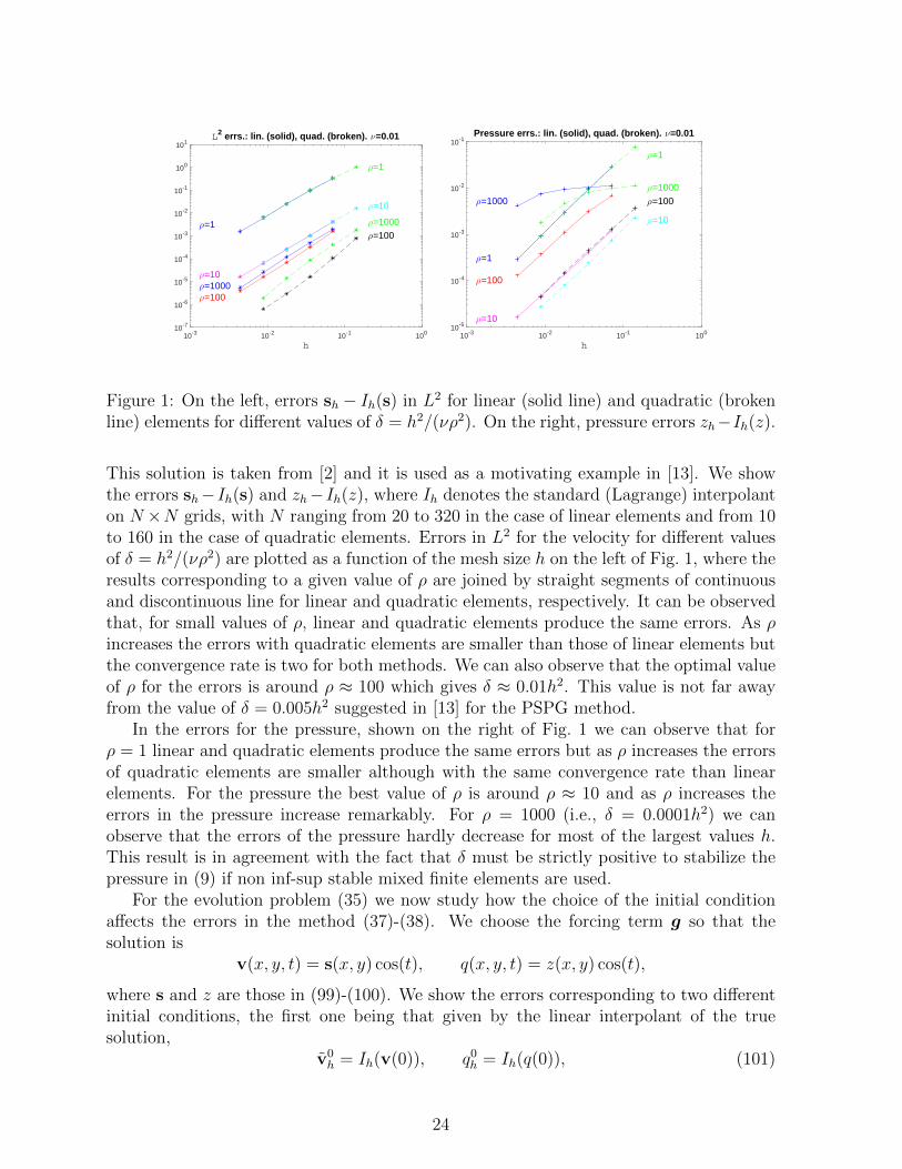
Figure 1: On the left, errors sh − Ih(s) in L2 for linear (solid line) and quadratic (brokenline) elements for different values of δ = h2/(νρ2). On the right, pressure errors zh−Ih(z).

This solution is taken from [2] and it is used as a motivating example in [13]. We showthe errors sh−Ih(s) and zh−Ih(z), where Ih denotes the standard (Lagrange) interpolanton N ×N grids, with N ranging from 20 to 320 in the case of linear elements and from 10to 160 in the case of quadratic elements. Errors in L2 for the velocity for different valuesof δ = h2/(νρ2) are plotted as a function of the mesh size h on the left of Fig. 1, where theresults corresponding to a given value of ρ are joined by straight segments of continuousand discontinuous line for linear and quadratic elements, respectively. It can be observedthat, for small values of ρ, linear and quadratic elements produce the same errors. As ρincreases the errors with quadratic elements are smaller than those of linear elements butthe convergence rate is two for both methods. We can also observe that the optimal valueof ρ for the errors is around ρ ≈ 100 which gives δ ≈ 0.01h2. This value is not far awayfrom the value of δ = 0.005h2 suggested in [13] for the PSPG method.

In the errors for the pressure, shown on the right of Fig. 1 we can observe that forρ = 1 linear and quadratic elements produce the same errors but as ρ increases the errorsof quadratic elements are smaller although with the same convergence rate than linearelements. For the pressure the best value of ρ is around ρ ≈ 10 and as ρ increases theerrors in the pressure increase remarkably. For ρ = 1000 (i.e., δ = 0.0001h2) we canobserve that the errors of the pressure hardly decrease for most of the largest values h.This result is in agreement with the fact that δ must be strictly positive to stabilize thepressure in (9) if non inf-sup stable mixed finite elements are used.

For the evolution problem (35) we now study how the choice of the initial conditionaffects the errors in the method (37)-(38). We choose the forcing term g so that thesolution is

v(x, y, t) = s(x, y) cos(t), q(x, y, t) = z(x, y) cos(t),

where s and z are those in (99)-(100). We show the errors corresponding to two differentinitial conditions, the first one being that given by the linear interpolant of the truesolution,

v0h = Ih(v(0)), q0

h = Ih(q(0)), (101)

24

10-6 10-4 10-2 100

t

10-4

10-3

10-2

10-1

100

101Pressure errors in L2 for Δt=δ

h= 2/20h= 2/40h= 2/80

Figure 2: Pressure errors pnh − Ih(p(tn)) for ∆t = δ y δ = h2/(100ν): Initial data (102)(solid line), and (101) (broken line).

and the second one that given by the stabilized Stokes approximation (8)-(9) to (7)

v0h = sh(0) q0

h = zh(0) (102)

where g is chosen so that the solution is v(0) and q(0). According to Remark 8, anyinitial data other than (102) should give an O(1) error in the pressure in the first step.This can be seen in Fig. 2, where we show the time evolution of the errors qnh − Ih(q(tn)),for δ = h2/(100ν) and decreasing values of h. It can be observed that whereas for initialdata given by (102) (joined by a solid line) the errors decrease with h already from thefirst step, they remain O(1) in the first step for initial data (101) (joined by a brokenline). Nevertheless, these O(1) errors decay very fast with time and, for a fixed t > 0 theydecay with h as well. Eventually, for t sufficiently large, they are indistinguishable fromthose corresponding to initial data given by (102).

References

[1] S. Badia & R. Codina, Convergence analysis of the FEM approximation of the firstorder projection method for incompressible flows with and without the inf-sup con-dition, Numer. Math. 107, (2007) 533–557.

[2] S. Berrone & M. Marro, Space-tiem adaptive simulation for unsteady Navier-Stokesequations, Comput. Fluids., 38 (2009), 1132–1144.

[3] R. Codina, Pressure Stability in Fractional Step Finite Element Methods for Incom-pressible Flows, J. Comput. Physics 170, (2001), 112–140.

[4] E. Burman & M. A. Fernandez, Analysis of the PSPG method for the transientStokes’ problem, Comput. Methods Appl. Mech. Engrg. 200, (2011) 2882–2890.

[5] A. J. Chorin, Numerical solution of the Navier-Stokes equations, Math. Comput. 22,(1968) 745–762.

25

[6] Philippe G. Ciarlet. The finite element method for elliptic problems , North-HollandPublishing Co., Amsterdam, 1978.

[7] P. Constantin & C. Foias, Navier-Stokes Equations , Chicago Lectures in Mathemat-ics. University of Chicago Press, Chicago, IL, 1988.

[8] J. de Frutos, B. Garcıa-Archilla & J. Novo, Error analysis of projection methods fornon inf-sup stable mixed finite elements. The evolutionary Navier-Stokes equations,submitted.

[9] J. de Frutos, V. John & J. Novo, Projection methods for incompressible flow problemswith WENO finite difference schemes, Journal Comput. Phys. 309 (2016), 368-386.

[10] J. L. Guermond & L. Quartapelle, On stability and convergence of projection meth-ods based on pressure Poisson equation, Inter. J. Numer. Methods Fluids, 26 (1998)1039–1053.

[11] J. L. Guermond, P. Minev & J. Shen, An overview of projection methods for incom-pressible flows, Comput. Methods Appl. Mech. Engrg. 195 (2006) 6011–6045.

[12] J. L. Guermond & L. Quartapelle, On the approximation of the unsteady Navier-Stokes equations by finite element projection methods, Numer. Math. 80, (1998)207–238.

[13] V. John & J. Novo, Analysis of the PSPG Stabilization for the Evolutionary StokesEquations Avoiding Time-Step Restrictions, SIAM J. Numer. Anal., 53 (2015) 1005–1031.

[14] P. D. Minev, A stabilized incremental projection scheme for the incompressibleNavier-Stokes equations, Inter. J. Numer. Methods Fluids, 36 (2001) 441–464.

[15] A. Prohl, Projection and Quasi-Compressibility Methods for Solving the Incompress-ible Navier-Stokes equations, Advances in Numerical Mathematics, B. G. Teubner,Stuttgart, 1997.

[16] A. Prohl, On Pressure Approximation Via Projection Methods for NonstationaryIncompressible Navier-Stokes Equations, SIAM J. Numer. Anal., 47 (2008) 158–180.

[17] R. Rannacher, On Chorin’s projection method for the incompressible Navier-Stokesequations, Lecture Notes in Mathematics, 1530, Springer, Berlin, 1992, 167–183.

[18] J. Shen, On error estimates of projection methods for Navier-Stokes equations: first-order schemes, SIAM J. Numer. Anal., 29 (1992) 57–77.

[19] J. Shen, Remarks on the pressure error estimates for the projection methods, Numer.Math., 67 (1994) 513–520.

[20] R. Temam, Sur lapproximation de la solution des equations de NavierStokes par lamethode des pas fractionnaires ii, Arch. Ration. Mech. Anal. 33 (1969) 377–385.

26