Source of AcquisitionNASA Johnson Space Center

Error Cost EscalationThrough the Project Life Cycle

AbstractIt is well known that the costs to fix errors increase as the project matures, but how fast do

those costs build? A study was performed to determine the relative cost of fixing errorsdiscovered during various phases of a project life cycle. This study used three approaches todetermine the relative costs: the bottom-up cost method, the total cost breakdown method, andthe top-down hypothetical project method. The approaches and results described in this paperpresume development of a hardware/software system having project characteristics similar tothose used in the development of a large, complex spacecraft, a military aircraft, or a smallcommunications satellite.

The results show the degree to which costs escalate, as errors are discovered and fixed atlater and later phases in the project life cycle. If the cost of fixing a requirements errordiscovered during the requirements phase is defined to be 1 unit, the cost to fix that error if foundduring the design phase increases to 3 — 8 units; at the manufacturing/build phase, the cost to fixthe error is 7 — 16 units; at the integration and test phase, the cost to fix the error becomes 21 —78 units; and at the operations phase, the cost to fix the requirements error ranged from 29 unitsto more than 1500 units.

IntroductionWe know that the cost to fix errors increases as a project matures — that it will cost more to

fix a requirements error after the product is built than it would if the requirements error wasdiscovered during the requirements phase of a project. So how important is it to the bottom-lineto find errors as early as possible — putting increased emphasis on systems engineering tasks inthe early stages of the project life cycle? Especially when schedule urgencies push the project torush through definition and start cutting metal? Increased emphasis on finding errors early in theproject life cycle means spending more time and a larger percentage of project costs in thedefinition phases of a project — more than is usually allocated to the early phases.

BackgroundMany published papers, articles, and books (cited in the following sub-sections) provide

information regarding the "value" of systems engineering and quantitative software cost factors,but few sources in the published literature define system cost factors. When relative cost-to-fixnumbers are published, it is difficult to discern the methods used to produce the results.

Cost Factors. In this paper, we will often refer to the term "cost factors." It is a term used inmany of the previous studies discussing the costs of errors in software systems, and is central tothe methodologies we used to analyze generic systems error costs. Cost factors representnormalized costs to fix an error. These factors may be used as a "yardstick" to measure orpredict the cost to fix errors in different projects.

Software Cost Factors. Barry Boehm performed some of the first cost studies to determine — bysoftware life cycle phase — the cost factors associated with fixing errors. Finding and fixing a

https://ntrs.nasa.gov/search.jsp?R=20100036670 2018-05-05T21:23:32+00:00Z

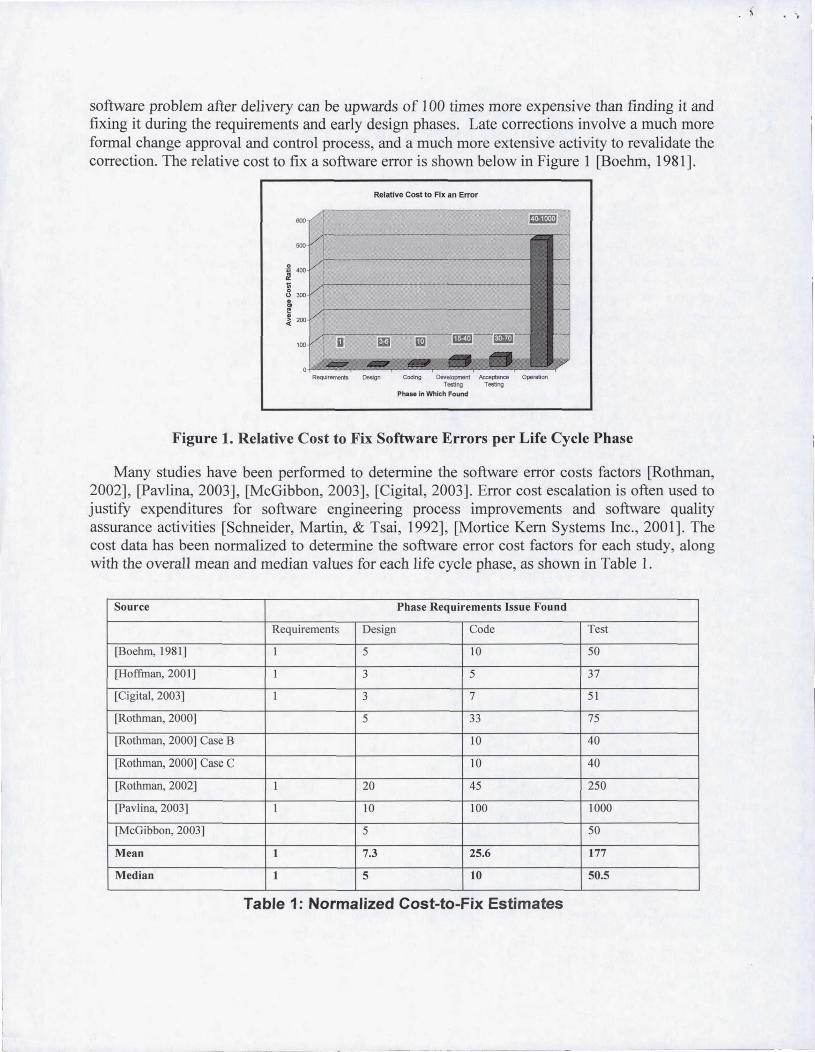
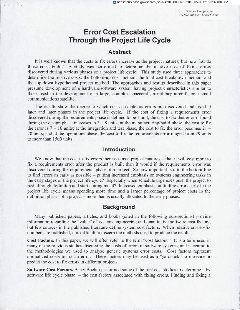
software problem after delivery can be upwards of 100 times more expensive than finding it andfixing it during the requirements and early design phases. Late corrections involve a much moreformal change approval and control process, and a much more extensive activity to revalidate thecorrection. The relative cost to fix a software error is shown below in Figure 1 [Boehm, 1981].

Figure 1. Relative Cost to Fix Software Errors per Life Cycle Phase

Many studies have been performed to determine the software error costs factors [Rothman,2002], [Pavlina, 2003], [McGibbon, 2003], [Cigital, 2003]. Error cost escalation is often used tojustify expenditures for software engineering process improvements and software qualityassurance activities [Schneider, Martin, & Tsai, 1992], [Mortice Kern Systems Inc., 2001]. Thecost data has been normalized to determine the software error cost factors for each study, alongwith the overall mean and median values for each life cycle phase, as shown in Table 1.

Source Phase Requirements Issue Found

Requirements Design Code Test

J Boehm, 19811 1 5 10 50

11 loffman, 2001 1 3 5 37

[Cigital, 2003] 1 3 7 51

1 Rothman, 20001 5 33 75

1 Rothman, 20001 Case B 10 40

1 Rothman, 20001 Case C 10 40

Rothman, 2002] 1 20 45 250

IPavlina, 20031 1 10 100 1000

[McGibbon, 2003] 5 50

Mean 1 7.3 2 5. 6 177

Median 1 5 10 50.5

Table 1: Normalized Cost-to-Fix Estimates

System Cost Factors. The only known published information on systems cost factors was foundin a book on designing cost-effective space missions [Cloud, Giffen, Larson, and Swan, 1999].These systems cost factors, shown in Table 2, represent the costs of fixing errors in electronicshardware. The costs are referenced without any description of the approach or method used togenerate the comparative cost numbers, therefore it is difficult to discuss similarities anddifferences between the costs in Table 2 and the results of this paper.

Phase that Change Occurs Resulting CostProduct Design $1,000Product Testin g $10,000Process Design $100,000Low-Rate Initial Production $1,000,000Final Production/Distribution $10,000,000

Table 2: Systems Cost Factors

Life Cycle PhasesFigure 2 maps the five life cycle phases, used in this paper, to the NASA project life cycle flow,and to the NASA and Department of Defense (DoD) acquisition phases. Major control gates, i.e.technical maturity milestones, are also shown in Figure 2. The NASA Systems Engineering LifeCycle [NASA SE Handbook, 1995] was used to categorize, by phase, the error discovery point.

NASA Mission Definition System Definition & Final Desigr Fabrication & Integration, Deployment & Mission

Project Preliminary Design Operational Verification Operations

Life CycleFloe

MaturityMilestones

MDR SDR PD CDR PRR EoA SAR ORR

NASA Phase A Phase B Phase C Phase 1) Phase E

Phases Preliminary Analysi Definition I Design I Development Operations

DOD Concept Exploration Demonstration Engineering & Manulacturing Production & Deployment Operations &

Phases & Definition & Validation Development Support

Project Requirements Design

IManufacturing/ Integration/Test Operations

Phases I Build

Figure 2. Project Phases in Relation to NASA and DoD Phases

Method 1 — Bottom-Up CostDescription. The bottom-up method of determining the cost to fix errors found in differentphases of the life cycle is derived from the most detailed form of cost estimation. The costs aregathered from every major discipline including all engineering groups, quality, contracts,vendors, logistics, program office, test, and many more. These costs and the schedule tocomplete the tasks are then rolled up into a total cost to fix the error and a total project schedule.Given the rolled up costs for several spacecraft modifications that were required to fix errors, theoverall error cost rates were estimated for each individual life cycle phase based on the bottom-up costs.

Methodology. This approach used the cost data from several spacecraft modifications. The costdata came in the form of total costs per modification per fiscal year and included a schedule forthe effort to complete the modifications. The activities throughout the entire project schedulewere consolidated into the five life cycle phases. The tasks were mapped to the suitable lifecycle phase, using the NASA Systems Engineering (SE) Handbook as a guide. For example,when a structures engineer included hours and schedule to recalculate the loads for a particularfix that added weight, these costs were included in the design life cycle phase. When the testengineer stated additional tests would have to be performed, that task was included within thetest phase. Every task included within the bottom-up approach was analyzed and checkedagainst the NASA SE Handbook and placed within the appropriate life cycle phase.

Assumptions. For each modification, the tasks required to fix the error were assigned to theappropriate life cycle phase. For the modification cost data, a percentage of individual fiscalyear labor and material costs was assigned based on the extent that each life cycle phaseoverlapped that particular fiscal year. For example, if 80% of a project's fiscal schedule wasrequirements tasks and the other 20% was design tasks, the fiscal year costs were separatedaccordingly. Once this was accomplished for all fiscal years, the life cycle phases were summedby adding their assigned percentage costs across the entire project.

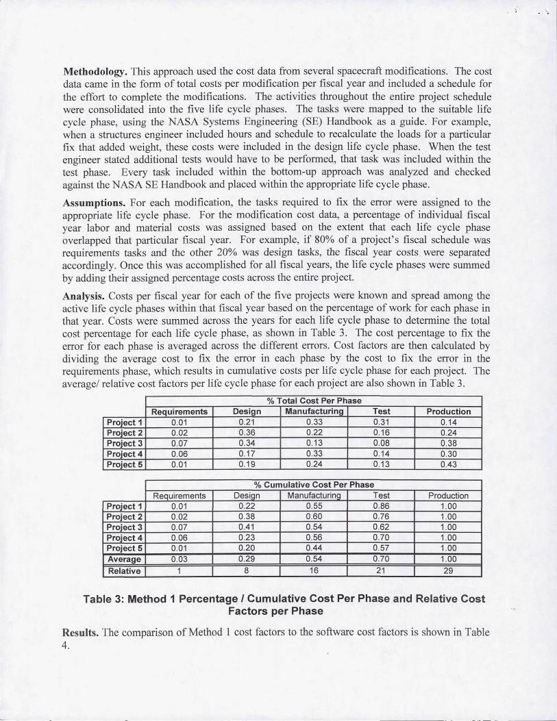
Analysis. Costs per fiscal year for each of the five projects were known and spread among theactive life cycle phases within that fiscal year based on the percentage of work for each phase inthat year. Costs were summed across the years for each life cycle phase to determine the totalcost percentage for each life cycle phase, as shown in Table 3. The cost percentage to fix theerror for each phase is averaged across the different errors. Cost factors are then calculated bydividing the average cost to fix the error in each phase by the cost to fix the error in therequirements phase, which results in cumulative costs per life cycle phase for each project. Theaverage/ relative cost factors per life cycle phase for each project are also shown in Table 3.

% Total Cost Per PhaseRequirements Design Manufacturing Test Production

Project 1 0.01 0.21 0.33 0.31 0.14Project 2 0.02 0.36 0.22 0.16 0.24Project 3 0.07 0.34 0.13 0.08 0.38Project 4 0.06 0.17 0.33 0.14 0.30Project 5 0.01 0.19 0.24 0.13 0.43

% Cumulative Cost Per PhaseRequirements Design Manufacturing Test Production

Project 1 0.01 0.22 0.55 0.86 1.00Project 2 0.02 0.38 0.60 0.76 1.00Project 3 0.07 0.41 0.54 0.62 1.00Project 4 0.06 0.23 0.56 0.70 1.00Project 5 0.01 0.20 1 0.44 0.57 1.00Average 0.03 0.29 0.54 0.70 1.00Relative 1 8 16 21 29

Table 3: Method 1 Percentage / Cumulative Cost Per Phase and Relative CostFactors per Phase

Results. The comparison of Method 1 cost factors to the software cost factors is shown in Table4.

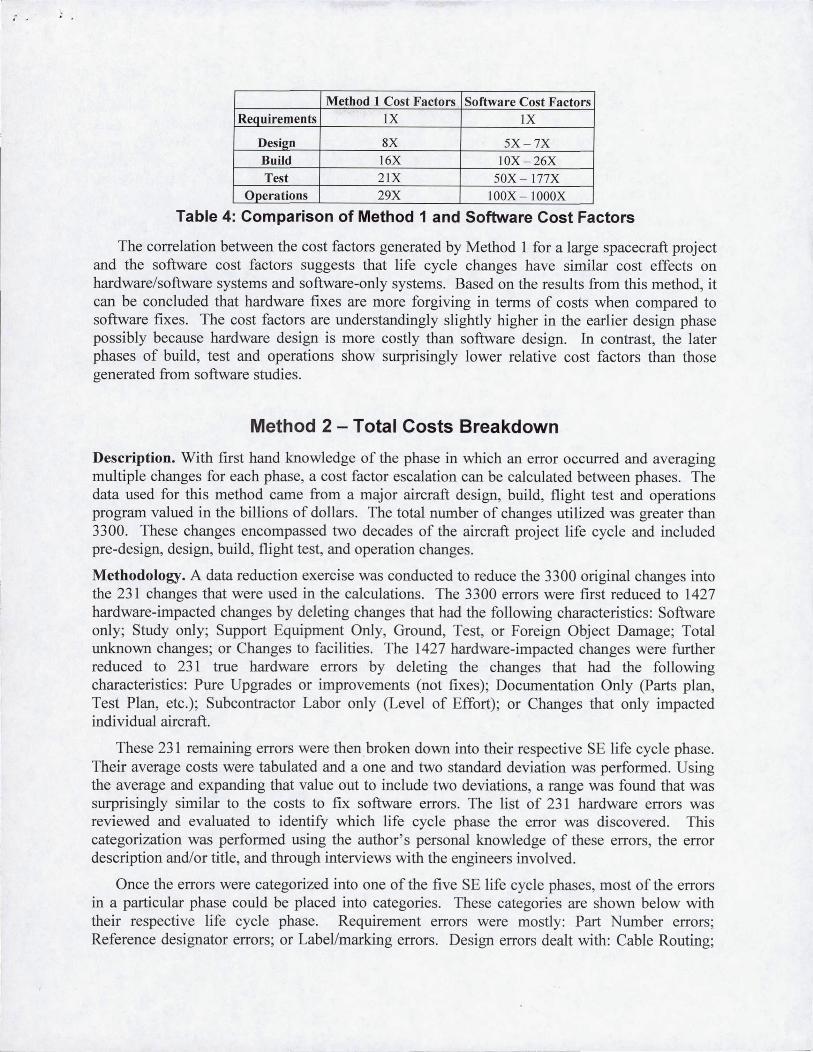
Method 1 Cost Factors Software Cost FactorsRequirements 1 X 1 X

Design 8X 5X — 7XBuild 16X I OX — 26XTest 21X 50X — 177X

O erations 29X I OOX — I OOOX

Table 4: Comparison of Method 1 and Software Cost Factors

The correlation between the cost factors generated by Method 1 for a large spacecraft projectand the software cost factors suggests that life cycle changes have similar cost effects onhardware/software systems and software-only systems. Based on the results from this method, itcan be concluded that hardware fixes are more forgiving in terms of costs when compared tosoftware fixes. The cost factors are understandingly slightly higher in the earlier design phasepossibly because hardware design is more costly than software design. In contrast, the laterphases of build, test and operations show surprisingly lower relative cost factors than thosegenerated from software studies.

Method 2 — Total Costs BreakdownDescription. With first hand knowledge of the phase in which an error occurred and averagingmultiple changes for each phase, a cost factor escalation can be calculated between phases. Thedata used for this method came from a major aircraft design, build, flight test and operationsprogram valued in the billions of dollars. The total number of changes utilized was greater than3300. These changes encompassed two decades of the aircraft project life cycle and includedpre-design, design, build, flight test, and operation changes.

Methodology. A data reduction exercise was conducted to reduce the 3300 original changes intothe 231 changes that were used in the calculations. The 3300 errors were first reduced to 1427hardware-impacted changes by deleting changes that had the following characteristics: Softwareonly; Study only; Support Equipment Only, Ground, Test, or Foreign Object Damage; Totalunknown changes; or Changes to facilities. The 1427 hardware-impacted changes were furtherreduced to 231 true hardware errors by deleting the changes that had the followingcharacteristics: Pure Upgrades or improvements (not fixes); Documentation Only (Parts plan,Test Plan, etc.); Subcontractor Labor only (Level of Effort); or Changes that only impactedindividual aircraft.

These 231 remaining errors were then broken down into their respective SE life cycle phase.Their average costs were tabulated and a one and two standard deviation was performed. Usingthe average and expanding that value out to include two deviations, a range was found that wassurprisingly similar to the costs to fix software errors. The list of 231 hardware errors wasreviewed and evaluated to identify which life cycle phase the error was discovered. Thiscategorization was performed using the author's personal knowledge of these errors, the errordescription and/or title, and through interviews with the engineers involved.

Once the errors were categorized into one of the five SE life cycle phases, most of the errorsin a particular phase could be placed into categories. These categories are shown below withtheir respective life cycle phase. Requirement errors were mostly: Part Number errors;Reference designator errors; or Label/marking errors. Design errors dealt with: Cable Routing;

Material changes for corrosion; Deletion of misc. hardware, un-needed seals, etc.; or Smoothnessissues prior to manufacturing. Manufacturing errors were mainly: Changes to hardware in orderto eliminate obstructions; Interference issues; Shimming requirements; or Hardwarereplacements. Testing errors included: Performance issues; Qualification test failures; or Re-qualification changes. Operations errors were found to be: Large errors found after delivery tothe field or Crew requested fixes.

Assumption. The Total Cost Breakdown method relied on facts and data obtained from personalknowledge of the major aircraft program, which was the subject of Method 2. Knowing whenthe aircraft entered flight test and was delivered to operations helped place errors within a certainlife cycle phase. For example, if the aircraft had not been delivered yet and an error wasdiscovered during flight, the error most likely occurred during the test phase. The earlier errorsthat occurred prior to the start of design were assumed to be errors that could be placed in therequirements phase. If manufacturing had not begun, it was assumed that the error belonged toone of the first two phases. Once the flight test milestone was passed, all errors were placed intothe operations phase.

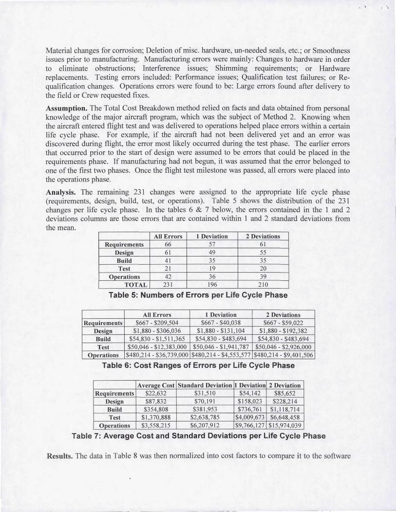
Analysis. The remaining 231 changes were assigned to the appropriate life cycle phase(requirements, design, build, test, or operations). Table 5 shows the distribution of the 231changes per life cycle phase. In the tables 6 & 7 below, the errors contained in the 1 and 2deviations columns are those errors that are contained within 1 and 2 standard deviations fromthe mean.

All Errors 1 Deviation 2 DeviationsRequirements 66 57 61

Design 61 49 55Build 41 35 35Test 21 19 20

Operations 42 36 39TOTAL 231 196 210

Table 5: Numbers of Errors per Life Cycle Phase

All Errors 1 Deviation 2 DeviationsRequirements $667 - $209,504 $667 - $40,038 $667 - $59,022

Design $1,880 - $306,036 $1,880 - $131,104 $1,880 - $192,382Build $54,830 - $1,511,365 $54,830 - $483,694 $54,830 - $483,694Test $50,046 - $12,383,000 $50,046 - $1,941,787 $50,046 - $2,926,000

O erations $480,214 - $36,739,000 $480,214 - $4,553,577 $480,214 - $9 ,401,506

Table 6: Cost Ranges of Errors per Life Cycle Phase

Average Cost Standard Deviation 1 Deviation 2 DeviationRequirements $22,632 $31,510 $54,142 $85,652

Design $87,832 $70,191 $158,023 $228,214Build $354,808 $381,953 $736,761 $1,118,714Test $1,370,888 $2,638,785 $4,009,673 $6,648,458

Operations $3,558,215 $6,207,912 $9,766,127 $15,974,039

Table 7: Average Cost and Standard Deviations per Life Cycle Phase

Results. The data in Table 8 was then normalized into cost factors to compare it to the software

1

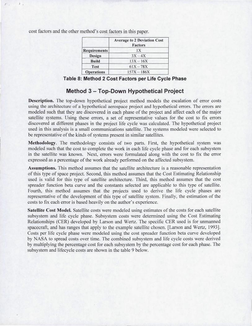
cost factors and the other method's cost factors in this paper.

Average to 2 Deviation CostFactors

Requirements 1XDesign 3X-4X

Build 13X — 16X

Test 61 X — 78X

Operations 157X — 186X

Table 8: Method 2 Cost Factors per Life Cycle Phase

Method 3 — Top-Down Hypothetical ProjectDescription. The top-down hypothetical project method models the escalation of error costsusing the architecture of a hypothetical aerospace project and hypothetical errors. The errors aremodeled such that they are discovered in each phase of the project and affect each of the majorsatellite systems. Using these errors, a set of representative values for the cost to fix errorsdiscovered at different phases in the project life cycle was calculated. The hypothetical projectused in this analysis is a small communications satellite. The systems modeled were selected tobe representative of the kinds of systems present in similar satellites.

Methodology. The methodology consists of two parts. First, the hypothetical system wasmodeled such that the cost to complete the work in each life cycle phase and for each subsystemin the satellite was known. Next, errors were formulated along with the cost to fix the errorexpressed as a percentage of the work already performed on the affected subsystem.

Assumptions. This method assumes that the satellite architecture is a reasonable representationof this type of space project. Second, this method assumes that the Cost Estimating Relationshipused is valid for this type of satellite architecture. Third, this method assumes that the costspreader function beta curve and the constants selected are applicable to this type of satellite.Fourth, this method assumes that the projects used to derive the life cycle phases arerepresentative of the development of this type of satellite system. Finally, the estimation of thecosts to fix each error is based heavily on the author's experience.

Satellite Cost Model. Satellite costs were modeled using estimates of the costs for each satellitesubsystem and life cycle phase. Subsystem costs were determined using the Cost EstimatingRelationships (CER) developed by Larson and Wertz. The specific CER used is for unmannedspacecraft, and has ranges that apply to the example satellite chosen. [Larson and Wertz, 1993].Costs per life cycle phase were modeled using the cost spreader function beta curve developedby NASA to spread costs over time. The combined subsystem and life cycle costs were derivedby multiplying the percentage cost for each subsystem by the percentage cost for each phase. Thesubsystem and lifecycle costs are shown in the table 9 below.

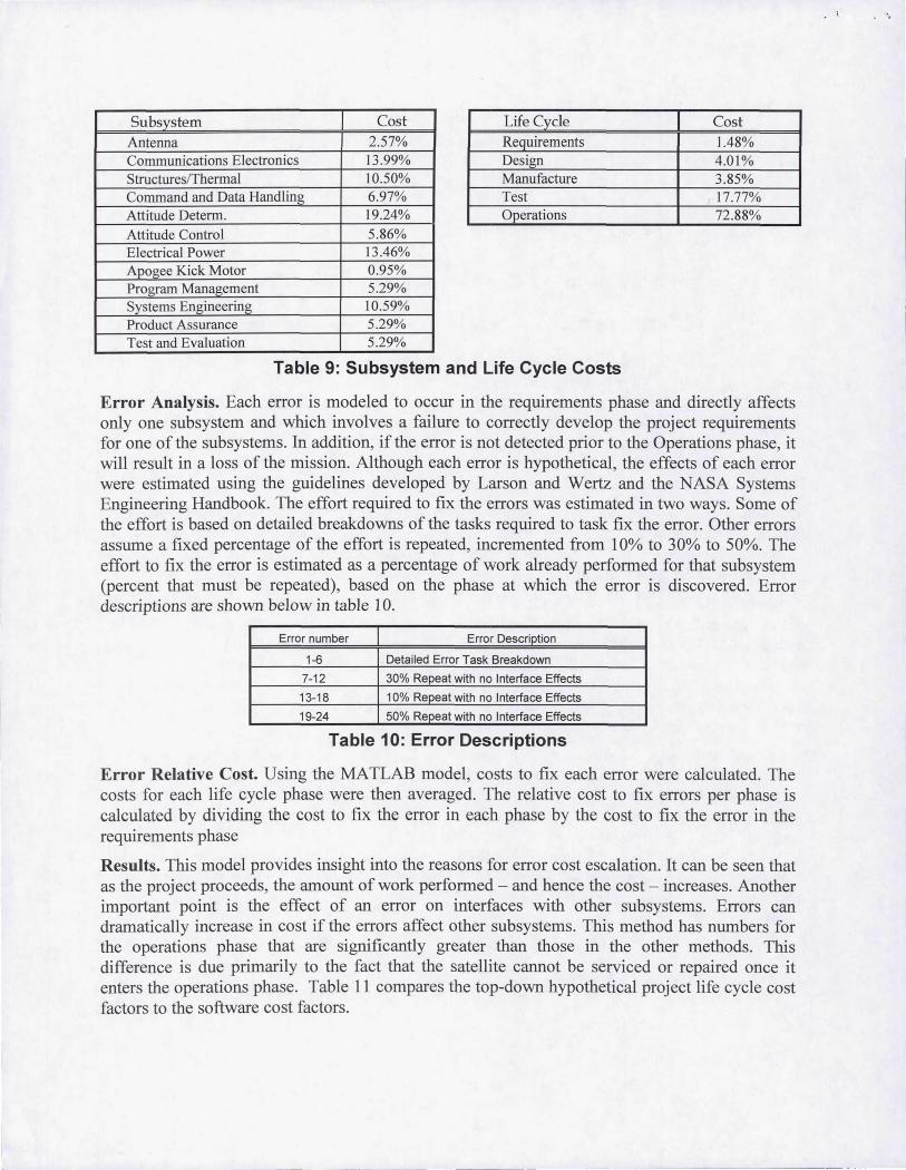
Subs stem Cost

Antenna 2.57%Communications Electronics 13.99%Structures/Thermal 10.50%Command and Data Handling 6.97%Attitude Determ. 19.24%Attitude Control 5.86%Electrical Power 13.46%Apogee Kick Motor 0.95%Program Management 5.29%Systems Engineering 10.59%Product Assurance 5.29%Test and Evaluation 5.29%

Life Cycle CostRequirements 1.48%Design 4.01%Manufacture 3.85%Test 17.77%Operations 72.88%

Table 9: Subsystem and Life Cycle Costs

Error Analysis. Each error is modeled to occur in the requirements phase and directly affectsonly one subsystem and which involves a failure to correctly develop the project requirementsfor one of the subsystems. In addition, if the error is not detected prior to the Operations phase, itwill result in a loss of the mission. Although each error is hypothetical, the effects of each errorwere estimated using the guidelines developed by Larson and Wertz and the NASA SystemsEngineering Handbook. The effort required to fix the errors was estimated in two ways. Some ofthe effort is based on detailed breakdowns of the tasks required to task fix the error. Other errorsassume a fixed percentage of the effort is repeated, incremented from 10% to 30% to 50%. Theeffort to fix the error is estimated as a percentage of work already performed for that subsystem(percent that must be repeated), based on the phase at which the error is discovered. Errordescriptions are shown below in table 10.

Error number Error Description1-6 Detailed Error Task Breakdown

7-12 30% Repeat with no Interface Effects13-18 10% Repeat with no Interface Effects19-24 50% Repeat with no Interface Effects

Table 10: Error Descriptions

Error Relative Cost. Using the MATLAB model, costs to fix each error were calculated. Thecosts for each life cycle phase were then averaged. The relative cost to fix errors per phase iscalculated by dividing the cost to fix the error in each phase by the cost to fix the error in therequirements phase

Results. This model provides insight into the reasons for error cost escalation. It can be seen thatas the project proceeds, the amount of work performed — and hence the cost — increases. Anotherimportant point is the effect of an error on interfaces with other subsystems. Errors candramatically increase in cost if the errors affect other subsystems. This method has numbers forthe operations phase that are significantly greater than those in the other methods. Thisdifference is due primarily to the fact that the satellite cannot be serviced or repaired once itenters the operations phase. Table 11 compares the top-down hypothetical project life cycle costfactors to the software cost factors.

:Method 1OMethod 2 L— BoundO Method 2 Upper Bound0Method 3

0

U

I 1

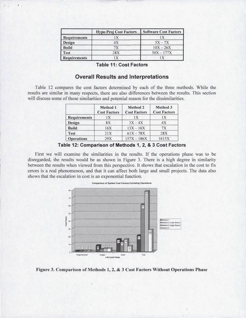
Hypo Pi2 Cost Factors Sof fare Cost FactorsRequirements IX IXDesign 4X 5X-7XBuild 7X 1 OX — 26XTest 28X 50X — 177XRequirements I X I X

Table 11: Cost Factors

Overall Results and Interpretations

Table 12 compares the cost factors determined by each of the three methods. While theresults are similar in many respects, there are also differences between the results. This sectionwill discuss some of those similarities and potential reason for the dissimilarities.

Method 1Cost Factors

Method 2Cost Factors

Method 3Cost Factors

Requirements 1X lX 1XDesign 8X 3X-4X 4XBuild 16X 13X — 16X 7XTest 21X 61X-78X 28XOperations I 29X I 157X — 186X 1615X

Table 12: Comparison of Methods 1, 2, & 3 Cost Factors

First we will examine the similarities in the results. If the operations phase was to bedisregarded, the results would be as shown in Figure 3. There is a high degree in similaritybetween the results when viewed from this perspective. It shows that escalation in the cost to fixerrors is a real phenomenon, and that it can affect both large and small projects. The data alsoshows that the escalation in cost is an exponential function.

Comparison of System Cost Factors Excluding Operations

Renu-menta Design Build TestLtfe-Cycle Phase

Figure 3. Comparison of Methods 1, 2, & 3 Cost Factors Without Operations Phase

o tn Software Lower

^EoSaflwereUpper

System Lower

System Upper

The results are also dissimilar in many ways. For example, methods two and three clearly donot give the same factors for the last three phases. Part of this can be explained by the nature ofthe errors used in method three. All of those errors were of such magnitude that if they were notdiscovered prior to the Operations phase, they would result in a loss of the entire system. Table13 compares the cost factors for software projects with those for systems projects; the systemscost factors shown are a composite of the results of the three methods used in this study. Thecomparison is shown graphically in Figure 4.

SoftwareCost Factors

SystemsCost Factors

Requirements 1 X 1 XDesign 5-7X 3X-8XBuild IOX-26X 7X-16XTest 50X-177X 21 X-78XOperations 100X-1000X 29X-1615X

Table 13: Comparison of Software & Systems Cost Factors

Comparison of Software and System Cost Factors

Requirements Design Build Test OperationsLife-Cycle Phase

Figure 4. Comparison of Software and Systems Cost Factors

Again, there are both similarities and differences to be seen in this cost data. The softwarecosts follow the same exponential trend as the systems costs. This is not surprising as in manyrespects software and systems are developed similarly. In addition, the upper bound of thesoftware operations phase cost factor is of the same order as the upper bound of the systemsoperations phase cost factor. This would seem to indicate that software systems are just asvulnerable to so called "killer errors", as are physical systems.

Recommendations

There are areas that could be improved upon in follow-on studies. First, with respect tomethods one and two, a greater sample size would clearly improve the accuracy of the results.The data used in this study was somewhat limited in quantity and with respect to the details ofthe errors involved. A future study could benefit from a larger sample size, and a greater depth ofknowledge concerning the errors to be analyzed. Another improvement that could be made iswith respect to the types of projects from which the data is collected. The real-world data used inthis study came from two large aerospace projects.

Future studies could examine data from both smaller aerospace projects and projects fromother sources such as the telecommunications, construction, and petrochemical industries. Thiswould give the resultant cost factors a much broader applicability. With respect to method three,future studies could also make improvements. First, the model should be validated bycomparison with actual errors. The model source data — including the cost estimatingrelationships — could be improved through this validation process.

Summary

This paper presents the results of a study on the escalation of the cost to fix errors as a projectmoves through its life cycle. The team used three methods to calculate the escalation in costs: thebottom-up cost method, the total cost breakdown method, and the top-down hypothetical projectmethod. In each of the methods, the costs were normalized to obtain cost factors. The studyrevealed that costs escalate in an exponential fashion. This paper demonstrates that earlydetection of errors is highly important to the success of any project.

ReferencesBoehm, B. W., Software Engineering Economics, Prentice-Hall, Englewood Cliffs, NJ, 1981.Cigital, "Case study: Finding defects earlier yields enormous savings," Available at

www.cigital.com, 2003.Cloud, Giffen, Larson, and Swan, "Designing Cost-Effective Space Missions: An Integrated,

Systems Engineering Approach," Teaching Science and Technology, Inc., 1999.Larson, W. and Wertz, J., Space Mission Analysis and Design, Second Edition, Microcosm, Inc.

and Kluwer Academic Publishers, Boston, 1993.MATLAB, Learning AIM TLAB, The MathWorks, Inc., January 2001.McGibbon, T., "Return on investment from software process improvement," Available at

www.dacs.dtic.mil , 2003.Mortice Kern Systems Inc., "From Software Quality Control to Quality Assurance," 2001.NASA Systems Engineering Handbook, SP-6105, National Aeronautics and Space

Administration, June 1995.Pavlina, S., "Zero-defect software development," Dexterity Software, Available at

www.dexterity.com , 2003.Rothman, J., "What does it cost to fix a defect?" StickyMinds.com, February 2002, Available at

http://www.stickyminds.com/stgeletter/archive/20020220nl.asp, 2003.Schneider, G. M., Martin, J., and Tsai, W. T., "An experimental study of fault detection in user

requirements documents," ACM Transactions on Software Engineering andMethodology, Vol 1, No 2, April, 1992, pp 188 — 204.