Error Diagnosis of Cloud Application OperationUsing Bayesian Networks and Online Optimisation

Xiwei Xu, Liming Zhu, Daniel Sun, An Binh Tran, Ingo Weber, Min Fu, Len BassSSRG, NICTA, Sydney, Australia

School of Computer Science and Engineering, UNSW, Sydney, Australia{firstname.lastname}@nicta.com.au

REGULAR PAPER

Abstract—Operations such as upgrade or redeployment arean important cause of system outages. Diagnosing such errors atruntime poses significant challenges. In this paper, we propose anerror diagnosis approach using Bayesian Networks. Each nodein the network captures the potential (root) causes of operationalerrors and its probability under different operational contexts.Once an operational error is detected, our diagnosis algorithmchooses a starting node, traverses the Bayesian Network andperforms assertion checking associated with each node to confirmthe error, retrieve further information and update the beliefnetwork. The next node in the network to check is selectedthrough an online optimisation that minimises the overall avail-ability risk considering diagnosis time and fault consequence.Our experiments show that the technique minimises the risk offaults significantly compared to other approaches in most cases.The diagnosis accuracy is high but also depends on the transientnature of a fault.

Keywords—Diagnosis; Cloud; Operation; Bayesian network;Online Optimisation

I. INTRODUCTION

Cloud applications are subject to many types of spo-radic system operations, such as upgrade, reconfiguration, on-demand scaling, deployment, and auto-recovery from nodefailures. Both the ease of such operations (programmablethrough Cloud infrastructure APIs) and the prevalence of con-tinuous deployment practices are significantly increasing thefrequency and simultaneousness of these operations. Recentempirical research [1] has shown that the majority of system-wide failures (i.e., outages) are caused by system operations,such as starting a service, adding a node to a running system,or restarting a node. Among the 9 categories of causes (inputevents) of system-wide failures, 69% are caused by operation-related activities. According to the same study, a large portionof outages are also caused by automated, cascading overre-actions to initial small errors – usually because the causewas not known and the automated fault-tolerance reactionssimply replaced erroneous resources, rather than fixing thecause. These observations were confirmed by another large-scale empirical study [2] of 3000 issues in cloud systems. Mostissues come from under-tested “operation protocols” (cloning,replication and recovery) rather than the primary features ofthe application. Also, a survey of 50 system administratorsfrom multiple countries concluded that 8.6% of operationsfail [3]. Some of these failures are due to unreliable Cloudinfrastructure APIs [4], [5]. Our own interviews with industryon outages (unpublished as yet) revealed several specificreasons. For example, one outage happened because newly

replaced VMs in an auto-scaling group (ASG) did not havean application installed properly. The corresponding healthcheck was misconfigured, which led to more and more healthyVMs being replaced by broken ones. Another outage happenedbecause VMs were terminated based on their age rather thancurrent workload, causing many heavily loaded VMs to beterminated.

Diagnosing these errors quickly, especially at runtime toallow better cause-aware recovery actions, poses significantchallenges. Most error diagnosis heavily relies on an operator’sexperiences, her familiarity with the system and a looselyordered diagnostic path. An operator would manually issue asequence of commands to acquire more information and assertwhether a particular candidate cause is the actual cause, untilan actionable (root) cause is identified. She would also digthrough logs and observe metrics and dashboards. This takesa significant amount of time. Meanwhile the failure persists, asdoes the cause, and cause-unaware recovery potentially keepsdoing more harm than good. This might be inevitable if theerrors and the causes are specific to the application itself.However, we have observed that:

1) Operations of application usually have a relatively smallerset of well-understood faults, especially if the operation ismanipulating course-grained VMs, lightweight containers,and application binaries, and if the configuration of themuses standard infrastructure facilities and APIs.

2) The operational context is an important input to diagnosis:it can guide diagnosis in the right direction. During specificparts of operations, certain types of (unreliable) APIsor activities are exercised more frequently. Therefore, anotherwise unlikely fault can suddenly become the mostlikely cause.

3) Error diagnosis takes time and can follow different diag-nostic paths. Deciding on the most efficient diagnostic pathto take should consider both the likelihood of the causesand the consequences, so as to minimise the risk.

Motivated by these observations, in this paper we propose anovel approach for automated diagnosis of non-transient faultsduring operations, i.e., faults that are still present when thediagnosis checks if they are present. The approach consistsof two parts: (i) a model of common operational issues, i.e.,faults/errors/failures, along with contextual, probabilistic, andrisk information about them; and (ii) an optimisation algorithmto select the best diagnostic path when an issue occurs. In moredetail, we use a Bayesian Network (BN) to model operational

issues as nodes in BN, the probability of them happening andthe dependencies among them. Each node also has a set ofassertions that can be run to confirm the presence of this issueat runtime, or to retrieve further information required for futurediagnostics. The online optimisation algorithm we devised re-evaluates the situation after each step, and selects the nextnodes whose assertions to check in a manner that minimisesrisk, e.g., that a significant fault is left undiagnosed for toolong. In the past, Fault Trees (FTs) [6] were used to assistdiagnosis without considering fault probability or risk. Ourapproach starts by converting such a FT to a BN, since theBN enables belief updates using runtime information and theconsideration of the above-mentioned additional factors.

The main contributions of this paper are:

• A BN-based model of operational issues (faults/errors/failures) and its association with assertion checking toenable runtime confirmation of the presence of issues.• Construction of a BN from a FT, with prior probabilities

for root causes collected from literature, historical data,and BN-driven derivation.• A diagnosis algorithm that traverses a BN to execute asser-

tion checking associated with BN nodes, and update belieffrom the assertion results. The algorithm also incorporatesthe concept of soft evidence to accommodate potentialfalse positives/negatives of assertion results.• An online optimisation algorithm that chooses a diagnosis

path that minimises risk within acceptable diagnosis time.

Our evaluation uses real outages encountered by industry,as captured in our interviews mentioned above. Comparativeexperiments show that the technique minimises the risk signifi-cantly compared to other approaches and meanwhile, maintainscomparable diagnosis time. For non-transient, known faults inour evaluation, we can achieve perfect diagnosis accuracy.

The paper outlines background information in Section II,followed by an overview of our approach in Section III.Section IV presents the construction of BNs from FTs, andSection V describes the online diagnosis, including belief up-dates, the diagnosis algorithm, and the diagnosis path selectionthrough optimisation. We evaluate our approach in Section VIand discuss the limitations in Section VII. Related work isdiscussed in Section VIII, and Section IX concludes the paper.

II. BACKGROUND

A. Bayesian Networks

BNs [7] are graphical models for reasoning about a domainunder uncertainty. The structure of the network captures quali-tative relationships between variables. In BNs, nodes representvariables (discrete or continuous) and directed arcs representcausal connection between variables.

BNs are used to predict the probability of unknown vari-ables and to update the probabilities when new knowledgearrives. In particular, when new values of some nodes areobserved, the probability of all the nodes can be updated byapplying Bayes’ Theorem. This process is called probabilitypropagation (or inference or belief update). Such new informa-tion is called evidence. There are different types of evidence:specific evidence, negative evidence, and virtual/soft evidence.Soft evidence is used to reflect the uncertainty in the evidence

itself. For example, if you should update a BN based on theevidence that someone tells you she does not smoke, there isa small chance she is lying. We use soft evidence to reflectthat runtime diagnostic assertions may return false results.

BNs and FTs are the most widely used techniques fordependability analysis. In comparison, BNs allow for morepowerful modelling and analysis. FTs are limited through theirstatic structure and in their uncertainty handling [8].

B. System Operation and Process Context

Applications in Cloud are subject to sporadic changesdue to operational activities such as upgrade, snapshotting,redeployment, restart, recovery, and replication among others.Some operations can be relatively long-lasting such as large-scale upgrade and reconfiguration. Multiple operations canhappen at the same time. There is a sporadic nature to theseoperations, as some are triggered by ad hoc bug fixing andfeature delivery while others are triggered periodically. Someoperations have significant impact at both the node level andthe system level. For example, upgrading could affect overallsystem capacity depending on the upgrade strategy, since anindividual virtual machine (VM) may be rebooted or replaced.The types of possible faults and their likelihood during suchoperations can be dramatically different when compared tonormal operation.

Our previous work took a process view of an operation[6]. Process context consists of the operations process id,instance id, the start and end time of operations, and theircharacteristics. Such process context can be captured in our BNmodel. The process models can be automatically mined fromthe logs produced by the operation [9]. Along with the processmodel, a set of regular expressions associated with each of thestep was generated to enable runtime mapping from observedlog lines to the current step in the process. Such detection ofoperation progression enables us to take process context intoconsideration. At runtime, the process context information canbe used in the BN model as evidence to adjust the occurrenceprobability associated with nodes – e.g., during a step whenVMs are rebooted, errors related to that are much more likely.

III. OVERVIEW OF THE DIAGNOSIS APPROACH

In this work, we want to consider fault occurrence proba-bilities, fault consequences, and the impact of diagnosis timecombined with fault consequence. We explain how BNs areused to capture the probabilistic causal relationships betweencontext, faults, and errors, how updates are handled, and howan online optimisation algorithm can minimise risk whenchoosing a diagnosis path.

Fig. 1 gives a graphical overview of our new approach.Firstly a BN is generated offline, either manually or from anexisting FT. In our case, the input FT is constructed based onour knowledge of common cloud operational faults, Cloud APIfaults, and system outages from real-world industry scenarios.Compared with BN, modelling an FT is more intuitive, andorganisations may have existing FTs as well as modellingexpertise. Thus, we devised a mapping algorithm – discussedin Section IV – that converts a FT into a BN and enriches itwith information such as (process) context and probabilities.

Offline

Online

Generate Bayesian Network

Update Belief

Select an Optimised Assertion

Run the Selected Assertion

- Fault Tree- Process Context- Probability (%)

Trigger Diagnosis

No more Assertion to run

- More evidence

Assert

- Assertion result

- Fault Probability- Risk + Fault Consequence + Checking Time + Assertion False Positive + Assertion False Negative

- Failed Assertion - Anomaly Detected by Monitor- Process Context

System

Fig. 1: Overview of Error Diagnosis Workflow.

The online diagnosis process is triggered when an anomalyis detected by some monitoring mechanism. The detectedanomaly and the current process context are the first evidence,based on which the BN updates the beliefs over the whole net-work, to adjust the occurrence probabilities of the intermediateerrors and root causes. Details of belief updates are discussedin Section V-A.

After the first belief updates, the set of BN nodes corre-sponding to the most urgent causes is determined, and assertionchecking for these nodes is started. Then, as the more and moreassertions return results, the belief is further updated basedon this new evidence. The diagnosis follows an algorithmtraversing the network. At any given time, the algorithmmaintains a to-check list of BN nodes: when the value of any ofthe nodes becomes known (by way of assertion checking) thatconfirms or denies the existence of particular faults or faultgroups. The current to-check list can be a sub-graph of theBN. It, too, is updated every time new evidence is received.The diagnosis terminates when there is no node left in theto-check list, or an actionable (root) cause is identified. It ispossible that no fault is found after the diagnosis stops. In thiscase, the error that was initially detected is caused by eithera transient fault or a false positive in error detection, or thediagnosis failed due to an incomplete BN. The details of thediagnosis algorithm are discussed in Section V-B.

There are different types of assertions. Assertions can beon-demand diagnostic checks that query the current state ofresources or systems (e.g., issuing a health check command onthe spot or querying the public cloud provider API for the cur-rent states of cloud resources). They can acquire informationfrom logs or other systems that already captured the desiredinformation. Assertions may also involve human operators,where the operator performs a check and provides the result ofthe assertion subsequently. On any path through the BN, a mixof these types of assertions may be encountered. Following thepath to confirm a particular fault may take considerable time,especially if a human needs to be in the loop.

It can be the case that multiple alternative paths could

diagnose a fault. Choosing a diagnosis path is done basedon the outcome of the optimisation algorithm below. Someassertions can proceed simultaneously, while others have tobe checked in sequence – e.g., when one assertion relies oninformation obtained by another assertion. It is usually notfeasible to assert the root causes directly due to assertiondependency, the very large state space of the whole system, andthe performance impact of investigating a larger state space.Just like a human operator, the semi-automated diagnosisusually follows few paths with limited concurrency. Wherean opportunity for concurrent checking exists, we could makeuse of it.

We use an online optimisation algorithm to choose thediagnosis path that presents the best trade-off, given thecurrent information. The optimisation algorithm selects thenext assertion(s) for the to-check list so that the diagnosis hasthe minimal risk through excluding the faults with higher riskfirst. The risk is calculated based on several factors includingthe probability and consequence of faults, the time requiredfor assertion checking to confirm a fault, and false posi-tive/negative rates of the respective assertion checking. Detailsof the optimisation algorithm are discussed in Section V-C.

IV. BAYESIAN NETWORK CONSTRUCTION

Our approach starts from a FT, and we produce a BN fromit. This is not the only pair of notations one could use, it is oneuseful choice, and we demonstrate its effectiveness. The initialnotation should be one that is widely used by practitioners (soexisting models in organizations can be used), and it shouldfacilitate communication among a range of stakeholders; FaultTrees have those features.

Mapping methods exist in the literature [8], [10], as dotools that support the conversion [11], [12]. We selected anexisting mapping method [8] and adapted it to integrate themodelling of (process) context. Fig. 2 illustrates the procedureused to construct the graphical structure of a BN from a FTand to generate prior and conditional probabilities for eachvariable. Currently, the one-off effort of converting a FT to aBN is done manually. We use Netica-J1 to construct the BN.

Graphical Mapping

Numerical Mapping

Root Fault Nodes

Intermediate Fault Nodes

Failure Nodes

Bayesian Network

Conditional Probability of

Root Fault Nodes

Conditional Probability Tables

of Intermediate Fault and Failure

Nodes

Process Context Nodes

Intermediate Events

Top Events

Primary Events

Fault TreeOther Information

Root Fault Occurrence

Probability under different Process

context

Boolean Gates

Operator Defined Process Context

Prior Probability of Process

Context Nodes

Process Occurrence Probability

Historical data

Fig. 2: Construction of Bayesian Network.

1http://www.norsys.com

A. Running Example

To illustrate our approach, we introduce a representativeerror/fault scenario. Say, one VM (or VM instance, or justinstance) is not using the expected version of an application.Such an error might cause anomalies at the application level oraccess problems. The example assumes the problematic VMis within an auto-scaling group (ASG), which is a commondeployment configuration on AWS (Amazon Web Services)2.ASGs help maintaining the availability of an application byautomatically scaling the capacity in or out, according touser-defined conditions. An ASG is always associated witha Launch Configuration (LC), which specifies how to launchVMs for the ASG. The LC includes information such as theAmazon Machine Image (AMI, i.e., from which VM imageto launch new VMs), ssh key pairs, security groups (SGs),and other configuration settings. An SG defines firewall ruleswhich control the traffic to or from the associated VMs.

Fig. 3 shows the relevant FT sub-tree for this scenario.The wrong application version in the problematic VM couldbe caused by an ill-configured LC (left-most branch). If thecurrent LC (denoted as LC’) is not the known correct LC, thatmay or may not be the root cause. To confirm LC’ is correct,all its fields need to have the same values as in LC. Otherproblems relate to settings for key pairs, SGs, and AMIs.

Wrong version of AMIRoot9

AND

Wrong key pairRoot2

VM uses a wrong versionFailure

OR

ASG is using LC' Root1

LC' uses wrong valueGate1

AND

Wrong Version of AMIRoot4

Wrong key pair IDGate2

Wrong security group ID Gate3

OR

Wrong AMI IDGate4

Wrong LC attached with ASGGate5

Attach the

instance to ASGRoot10

Wrong setting of SGRoot3

Wrong setting of SGRoot7

AND

Attach the

instance to ASGRoot8

Wrong key pair

IDRoot5

AND

Attach the

instance to ASGRoot6

Fig. 3: Fault Tree of the running example.

B. Graphical Mapping

In graphical mapping, the primary, intermediate, and topevents of the FT are converted into the root fault nodes,intermediate fault nodes, and failure nodes in BN. Takingthe semantics of the primary events and Boolean logics fromthe FT, all resulting BN nodes are binary: True or False.Fig. 4 shows the BN from converting the sub-tree given above.The nodes in the BN are connected in the same way as thecorresponding events in the FT.

We model process context (PC) as a set of nodes –shown in blue in Fig. 4. Each process context node representswhether a process or a major step of a process is currentlyexecuted or not. The figure shows two examples: the solidblue node models rolling upgrade, and the faded blue nodemodels another process context that affects VM-level faults.The system operator decides what types of processes are

2http://aws.amazon.com

Other process contextPC2

Wrong key pairRoot2

ASG is using LC'Root1

LC' uses wrong value

Gate1

VM uses a wrong versionFailure

Rolling Upgrade

PC1

Wrong LC attached with ASGGate5

Wrong AMI versionRoot4

Wrong key pairRoot5

Wrong AMI ID

Gate4

Instance is attached to

ASGRoot6

Wrong security group IDGate3

Wrong version of

AMIRoot9

Wrong key pair IDGate2

Wrong SG settingRoot7 Instance is

attached to ASGRoot8

Instance is attached to

ASGRoot10

Wrong SG settingRoot3

Fig. 4: Bayesian Network of the running example.

interesting enough to be explicitly modelled in the BN, andwhat the proper granularity, typically based on the impact ofa certain process or step on the occurrence probability of thefaults. Other contexts of interest can be modelled using thesame method.

The arrows between the process context nodes and theroot fault nodes represent the causal relationship between theprocess/step and the occurrence of the root faults. The effect ofthe process context on the occurrence of the intermediate faultsand failure is implied by the conditional probability. Contextnodes are binary with two values: on or off.

C. Probability Acquisition

The prior probabilities for some of the root faults and(process) context can be taken from the documentation of com-mercial products or from the literature, e.g., experiments [5]and empirical studies [1], [3], [4], [13]. Prior probabilitiesof remaining root faults can be calculated based on systemoperation scenarios. We classified the (root) causes into threemain categories: human error, virtual resource failure, and APIfailure. We do not consider hardware failures separately in ourapproach, since these are masked to the consumers of publicclouds and thus covered by the probability of virtual resourcefailure. Below we show how to calculate prior probabilitiesfor average operators and assuming AWS cloud services. Fordifferent environments, different base data needs to be used.

For Human error, we refer to the examples of humanerror probabilities included in [14]. In the context of systemoperation, human interactions with the system occur duringconfiguration, operation, diagnosis and system recovery. Weonly consider configuration and operation since our scope iserror diagnosis after a system fails. We assume 8.6% of systemoperations fail based on a survey from multiple countries [3],where most of the participants had more than 5 years of expe-rience. An extensive set of experiments are conducted in [13]to better understand the occurrence probability, category, andimpact of human errors. They identified 7 fault categories from42 faults found in 43 conducted experiments. 5 out of 7 faultcategories are within our scope: unnecessary restart of SWcomponent, start of wrong SW version, incorrect restart, globalmisconfiguration, local misconfiguration. The probability of acertain type of fault is estimated by multiplying the occurrencerate of the fault and 8.6%.

Virtual resource failure is a common problem on cloudinfrastructure due to various sources of uncertainty. We assumethe availability of AWS EC2 is the same for AWS availabilityzones at 99.95%, and the availability of ELB(Elastic Load Bal-ancer) and AMI(Amazon Machine Images) to be the same asS3(Simple Storage Service) at 99.99%. The failure probabilityis 1− availability. The age of a resource also has impact onits failure probability. In an empirical study investigating thefaults causing catastrophic failures on distributed systems [1],one finding shows that a recently restarted/added node has thehigher failure probability compared to other running nodes.Among the identified 9 categories of input events (causes) tofailures, starting/restarting/adding a new node together cover45.3% of all failures [1][Table 4]. Thus, we distinguish recentlymanipulated nodes from other running nodes with differentprior probabilities, by increasing failure probability for them.

Cloud API failures represent a large percentage of er-rors/failures on cloud applications. For example, more thanhalf (53%) of the error cases reported in Amazon’s EC2 forumare related to API failures [4]. We assume that the probabilityof API failure is P(API failure) = 53%*8.6%=4.6%.

The relationships between connected nodes are quantifiedthrough assigning conditional probability distributions. In ourscenario we only consider discrete variables, and thus distri-butions take the form of conditional probability tables (CPTs).Table I gives a sample CPT for root fault node ASG is usingLC’. The parent set of the root fault nodes contains the contextnodes PC1 and PC2. In the CPT, the probability for both values(True or False) for the chosen node is symbolised as Pi, underthe condition of one of the possible combinations of values ofPC1 and PC2. The LC associated with ASG is more likely tobe changed during rolling upgrade, thus P1 > P3 and P2 > P4.

TABLE I: Sample CPT of root fault nodes

Rolling Upgrade (PC1) On On Off OffOther process context (PC2) On Off On Off

P (Root Fault=True | PC1, PC2) P1 P2 P3 P4

P (Root Fault=False | PC1, PC2) 1-P1 1-P2 1-P3 1-P4

Sometimes the impact of an operations process can becalculated when historical data is sparse. For example, if anoperation calls a cloud API 12 times to manipulate resourceswithin 8 minutes. During the operation, the occurrence prob-ability of API failure increases and that can be calculated.

Acquiring probability is a challenging problem in prac-tice. Acquiring probability from literature has the problemof coverage and context relevance. The empirical studies wereferred to have different contexts and scopes. None of themcan be regarded as comprehensive, in that it would cover allthe possibilities and provide accurate distributions. However,precise probabilities are not necessarily required for accuratediagnosis, in our observation. The intuition is that certainoperations processes significantly increase certain types oferrors. As long as the relative ranking and the magnitude isreasonable, the diagnosis is relatively accurate. Adjustment tothe probabilities can be made based on specific operationalcontexts.

D. Numerical Mapping

The numerical mapping derives a CPT for each of theintermediate fault and failure node, according to the type ofgate present in the FT. Table II shows how the probabilityof intermediate faults with different logic gates are calculatedfrom the parent set, again for the left-most branch in Fig. 3.

TABLE II: Probability calculation of the running example

FT Node FT Node Type BN Probability (=True)Root1 Root fault Pr1

Root2 Root fault Pr2

Root3 Root fault Pr3

Root4 Root fault Pr4

Gate1 Intermediate fault (OR-gate) Pg1=1-(1-Pr2)×(1-Pr3)×(1-Pr4)Gate5 Intermediate fault (AND-gate) Pg2=Pg1×Pr1

V. RUNTIME DIAGNOSIS

A. Belief Update Using Assertion Results as Evidence

As mentioned in Background section, BN supports differ-ent types of evidence. In our scenario, the diagnosis approachcan receive both specific evidence and soft evidence.

1) Specific Evidence: Specific evidence refers to a definitefinding that a node has particular value. When the diagnosisprocess is triggered, that triggering message contains the firstsets of evidence: either a failed assertion or an anomalydetected by the monitoring mechanism, as well as (process)context information. All three can be considered definite inour current context, and thus considered specific evidence.In different contexts, this assumption can be dropped easily.The posterior probability or belief of the corresponding faultnodes (denoted as Bel(Fault)) are then either 0% or 100%.Once updated with specific evidence, Bel(Fault) is fixed, whichcannot be changed any more.

2) Soft Evidence: Not all received evidence is definite.Evidence can be given as a probability distribution over thevalues of the corresponding node, which is known as softevidence. Our approach assumes that assertions can havefalse positives/negatives in their results, and so the evidencegathered from them is taken as soft evidence.

Every fault, either root fault or intermediate fault, canbe associated with multiple assertions. The occurrence ofthe fault is confirmed or ruled out through these on-demandassertions. For each assertion, we calculate the false positiveand false negative rates from historical data. The reasons forinaccuracies in assertion results lie in the characteristics of thefault or the limitations of a certain assertion. For example, ifthe fault is transient, it is possible that by the time we doassertion checking, the fault already disappeared. To handlethis issue, false positive/negative rates of assertions need tobe considered with the evidence they present. Specifically,we denote an assertion’s false positive rate as Pfp > 0 andfalse negative rate as Pfn > 0. When receiving a positiveassertion result, the occurrence of the fault is confirmed with(1 − Pfp), and the occurrence of the fault is ruled out with(1−Pfn). After receiving an assertion result as a soft evidence,Bel(Fault = T ) is updated through applying Bayes’ Theoremas shown below. Assume we have:

P (Fault = T ) = PF , P (Fault = F ) = 1− PF (prior probability)P (A = T |Fault = F ) = Pfp (false positive rate of assertion)P (A = F |Fault = T ) = Pfn (false negative rate of assertion)P (A = F |Fault = F ) = 1− Pfp

P (A = T |Fault = T ) = 1− Pfn

where A represents Assertion. The belief in the fault occur-rence can in general be calculated as:

Bel(Fault = T )

= P (Fault = T |A)

=P (A|Fault = T )P (Fault = T )

P (A)

=P (A|Fault = T )P (Fault = T )

P (A|Fault = T )P (Fault = T ) + P (A|Fault = F )P (Fault = F )

Once a positive assertion result is received, this changes to:

Bel(Fault = T ) =(1−Pfn)PF

(1−Pfn)PF+Pfp(1−PF )

If the assertion result is negative, the belief becomes:

Bel(Fault = T ) =PfnPF

PfnPF+(1−Pfp)(1−PF )

After being updated with soft evidence, Bel(Fault) is notfixed: it can be further updated when more soft evidence frommore associated assertions is received. The question then is:what should be the threshold on probability to assume theoccurrence of the fault? This is a configurable setting in ourapproach. Operators may e.g. feel confident to assume a faultoccurred if Bel(Fault = T ) is higher than 90%.

3) Partial Belief Updates – Running Example: Table IIIshows how the beliefs are updated in the left-most branch ofthe running example based on different types of evidence.

TABLE III: Belief updates in the running example

Belief Root1 Root2 Root3 Root4 Gate1 Gate5No evidence .0330 .0361 .0361 .0361 .1041 .0037Failure=T .6563 .2369 .2369 .2369 .6809 .6461

PC1=T .8907 .3224 .3224 .3224 .9051 .8850Gate1=T .9778 .3562 .3562 .3562 1 .9778

Soft evidenceof Root3

.9778 .3745 .3156 .3745 1 .9778

Root4=T .9778 .0656 .0553 1 1 .9778Root1=T 1 .0656 .0553 1 1 1

The first row shows the beliefs before receiving anyevidence. Once the diagnosis is triggered by a failure, allthe beliefs increase dramatically. Along with the evidence offailure, evidence of process context PC1 is also received, andthe beliefs update results in all nodes within the left-mostbranch getting higher belief than the other branches. Amongthe six nodes, Gate1 has the highest belief, thus, we cancheck the assertion associated with Gate1 first. The receivedspecific evidence confirms that Gate1 is true, which meansRoot2, Root3 or Root4 must have occurred. Since the threehave the same belief, we randomly choose Root3 first. Thecorresponding assertion returns soft evidence against Root3,causing the belief of Root3 to be lowered. We then pick Root4for the next check, and the returned assertion result confirmsits definite occurrence. Since Gate1 is under an AND gate withRoot1, we also check the assertion associated with Root1, andfinally find out the root causes: Root1 and Root4.

B. Diagnosis Process

The BN is a graph G(V,E). A subset of vertices representthe possible root causes, R = {vri }, R ⊂ V . The goal ofdiagnosis is to identify the final set root causes Rf ⊂ R. Thediagnosis process traverses over some or all nodes other thanthe process context nodes. Each vertex vi is associated witha probability pi, which changes through belief updating. vi isalso associated with assertions, aij , 1 ≤ j. Calling each aijreturns either specific evidence in binary form (true or false),or soft evidence in form of a probability distribution over trueand false.

Algorithm 1 captures the diagnosis process. When a di-agnosis is triggered, it receives the values for context nodesand a failure node for the detected error as specific evidence.Bel(PC) and Bel(failure) are updated and fixed accordingly(line 1). ToDo is the current to-check list of nodes, i.e., theassertions associated with nodes in this list need to be evaluatedto find the (root) causes. V \ PC is the set of intermediatefault nodes and (root) cause nodes in BN. Initially, all theintermediate fault nodes are added to ToDo (line 2), whichis updated as the diagnosis proceeds and more evidence isreceived.

The diagnosis stops when ToDo is empty (line 3). Whilethere are nodes left in ToDo, we firstly select a node vifrom ToDo (line 4). The selection algorithm uses our onlineoptimisation, as discussed in the next section. There are simplealternative selection methods – e.g., just selecting the nodewith the highest probability from ToDo (as shown in theexample of Table III), or selecting a node based on a pre-defined diagnosis runbook, as a human operator would usuallydo. We compare these three methods in our evaluation.

If vi is a gate and if the belief of its parents (denoted asparents(vi)) is fixed (line 5), Bel(vi) can be calculated fromthe belief of its parents (line 6). Thus, no assertions need to bechecked and vi is removed from ToDo (line 7). Otherwise, anassertion associated with vi is executed. Algorithm 1 doesn’tconsider any attributes of assertions, it selects an assertionassociated with the node. Bel(vi) is updated based on theassertion result (lines 9-10). If the assertion result is specificevidence, Bel(vi) is fixed and vi is removed from ToDo (line12); else, Bel(vi) may still be updated later on.

If the assertion result confirms the condition of vi is true,lines 15-19 treat the case if vi is a (root) cause node. Therecan be consecutive AND gates along the path from vi to thefailure node, which means vi might not be the only root cause(lines 16-18). Thus, vi is pointed to the furthest AND gate.Please note that BN doesn’t have AND/OR gates, we keep thesemantics of gates from FT. We use child(vi) function to referto the child node of vi. Since the BN is converted from a faulttree, every node on our BN has at most one child. At line20, the (root) cause must be within the subGraph(vi), a subgraph of G defined as follows. subGraph(v)’s only leaf nodeis the current v from line 20, and root nodes in the subgraphare the (root) cause nodes that can be reached from v. Sincethe cause is confirmed to be in this subgraph, any node v′i inToDo is removed from ToDo if it is not in subGraph(vi) orif Bel(v′i) cannot be changed anymore (line 22).

If the assertion result confirms the condition of vi is false,it means the (root) cause is not within the subGraph(vi) (line

25). Similarly as before, if there are consecutive AND gatesalong the path from vi to the failure node, it means the rootcause is not in the subgraph with the furthest AND gate as theroot (lines 26-28). Thus we iterate through ToDo to removethe nodes with fixed belief, and the nodes that are containedin the subgraph (line 30). The belief of the nodes is updatedbefore removing them from ToDo. After the diagnosis processstops, all the (root) cause nodes with Bel(v = true) >=threshold are the root causes (Line 38).

C. Assertion Selection Optimisation

A critical step in the diagnosis process concerns whichnode from the to-check list to visit next. We present ourapproach for risk minimising selection in the following.

1) Attributes: We consider several attributes of both faultsand associated assertions in our optimisation method. Theattributes of faults/failures include occurrence probability,expressed by the belief of the corresponding node in theBN, and potential impact to the whole system, measured bypartial capacity loss. The attributes of assertions includeassertion execution duration and false positive / negativerates. Assertions have false positive and false negative ratebecause of the uncertainty during the measurement/assertingthat affects accuracy. As mentioned earlier, false positive andfalse negative rates are accounted for in the BN through beliefupdating using soft evidence.

The potential partial availability loss is calculated by mul-tiplying the duration of the assertion and the potential impactof the fault. Note that the total downtime includes detection,diagnosis, and recovery time. However, in the scope of thispaper we can only affect diagnosis time, and hence target solelyit in the optimisation. As mentioned earlier, there can be astrong need for human involvement to augment the automatedassertions, which may take considerable time. For example,once the LC is asserted to be not consistent with what weexpect after running automated checks, we may need a humanoperator to confirm that the current LC in use is indeed wrong,rather than a legitimate new one from a concurrent update.

2) Problem Analysis: Our target is to minimise the lossof capacity during the overall diagnosis process. Thus, thequestion is how to optimally select the next assertion(s)accordingly. Faults in our setting may have very differentconsequences. A fault in an individual VM may not have majorconsequences in a large-scale system. In contrast, a system-wide misconfiguration affecting all newly-added VMs mayhave major consequences.

According to the classic risk definition, e.g. [15], riskis calculated as the likelihood of an event multiplied withthe potential consequence. To this end, each vertex vi in Ghas an occurrence probability pi and is assigned cri , a realnumber denoting the relative capacity loss if the respectivefault / root cause is present. A successful diagnosis processtraverses a particular set of vertices, S ⊂ V . Note that theremay be more than one root cause, i.e., multiple {vri } in S.Say, vertex vk is being considered, and Sk is the set ofnodes reachable from vk, i.e., a path exists from vk to anyvi ∈ Sk. We then define the maximal root cause capacityloss as cmaxk = max(cri |vri ∈ Sk). At any point in time,our goal is to minimise the overall diagnosis time multiplied

Algorithm 1: diagnosis processInput: Evi(PC), Evi(Failure)Output: Rf , the final root causesData: G(V,E), the graphData: PC, the process context nodesData: R, the root cause nodesData: ToDo, the current to-check listData: aij , the jth assertion associated with vertex viData: Threshold, the threshold probability used to

decide root causeFn: Evi(v) is the evidence received on vFn: Bel(v) is the belief of vFn: Parents(v) is the parent set of vFn: Child(v) is the child of v

1 update Bel(PC), Bel(Failure)2 ToDo← V \ PC3 while ToDo 6= ∅ do4 vi, aij ← select vertex from ToDo and one of its

assertions5 if vi is Gate && Bel(Parents(vi)) is fixed then6 update Bel(vi)7 ToDo← ToDo \ {vi}8 else9 Evi(vi)← run aij

10 update Bel(vi)11 if Evi(vi) is specific evidence then12 ToDo← ToDo \ {vi}13 end14 if Evi(vi) == true then15 if vi ∈ R then16 while child(vi) is an AND Gate do17 vi = child(vi)18 end19 end20 for each v′i ∈ ToDo do21 if v′i /∈ subGraph(vi) || Bel(v′i) is fixed

then22 ToDo← ToDo \ {v′i}23 end24 end25 else26 while child(vi) is an AND Gate do27 vi = child(vi)28 end29 for each v′i ∈ ToDo do30 if v′i ∈ subGraph(vi) || Bel(v′i) is fixed

then31 update Bel(v′i = true)← 032 ToDo← ToDo \ {v′i}33 end34 end35 end36 end37 end38 Rf ← {vi|vi ∈ R and Bel(vi = true) >= Threshold}39 return (Rf )

by the maximal capacity loss, denoted as the consequenceC = maxvk∈ToDo(c

maxk ×

∑vi∈Sk,∀j tij), where tij is the

time spent on evaluating assertion aij .

The challenge in solving this optimisation problem liesin the uncertain information before the next assertion(s) isselected. This is two-fold: (i) the posterior probabilities will beupdated only after we have the evidence acquired by the asser-tion; (ii) the eventual (root) causes Rf are unknown before theend of the diagnosis. The closest problem in literature is thewell-known dynamic online shortest path problem, in whichthe weights of edges are unknown (unweighted) or vary withina range [16]–[18]. This is similar to our optimization problem,because accumulating tij to a minimum along a successfuldiagnosis path is similar to find a shortest path. To the best ofour knowledge, dynamic online shortest path is closest to ourproblem, but the algorithms to shortest path do not apply dueto the following differences. First, in most online shortest pathproblems, there is no dependency among the weights, but inour problem there are strong dependencies. Second, to solvethe shortest path problem it is sufficient to find such a shortestpath, but in our problem even if

∑vi∈S,∀j tij is minimised we

need to consider cmax. Third, Rf and cmax are known onlyafter the diagnosis process completed. Fourth, aij cannot besimply deemed as a part of weight. Hence, on the one hand theexisting algorithms for online shortest path do not apply for theoptimal selection of next assertions, and on the other hand toknow all posterior probabilities the BN requires 2|V |−1 updates(an assertion returns true or false, but the initial vertex doesnot need to be asserted). For these reasons we had to devise anovel online heuristic algorithm, which is described next.

3) Online Assertion Selection: Theoretically, one couldcheck assertions on all potential (root) causes, in a randomorder, until a positive assertion result is found. Such a randomwalk would often lead to suboptimal results, due to failureimpact and state space size. For a random walk, one cancalculate an expected value for C. When |R| is reasonably big,by introducing BN C should be much smaller than for randomwalk. Another naı̈ve method is a brute force exhaustive searchon G, but that would be even worse than a random walk, since|V | > |R|.

Instead, we propose a heuristic search approach, based onposterior probabilities and consequence C. Thus we introducea new feature for each vertex in G, called risk:

K = C × P

with C as defined above (maximal capacity loss for a diagnosispath) and P as the probability of finding the (root) cause onsuch a diagnosis path. It is not realistic to find the globaloptimum for either C and P . Therefore we propose onlineheuristic algorithm aiming at local optimum. In particular, wedefine Kij to each assertion, that is, the risk associated withassertion aij . The basic idea of our online heuristic algorithmis to select next assertion with a limited clairvoyance on thefuture risk. To do this, we define dm to be the maximum out-degree in G and dp the depth to which the algorithm shouldlook forward. Algorithm 2 basically computes the biggest Kij

from the candidate assertions for nodes in the to-check list.

Algorithm 2 is run for each vertex in the ToDo list. Foreach run, the set of possible nodes with assertions within the

Algorithm 2: dp-depth selection of the next assertionInput: current vertex vc from ToDo listOutput: next assertion aijData: G(V,E)Data: the clairvoyance depth dp to look forward

1 VR ← vi,∀d(vc, vi) ≤ dp − 1 and vi 6∈ R ; // all verticeswithin the distance dp − 1

2 FV ← vi,∀d(vc, vi) ≤ dp or vi ∈ R ; // front vertices, allvertices with the distance dp

3 Pt ← all paths from vc to vi ∈ FV ; // all paths from vcto the front vertices within the clairvoyance

4 Kmax ← 0; // maximal risk initiated to be 05 amaxij ; // the assertion with the maximal risk6 counter ← 0 ; // count to the number of all possibilities

within the clairvoyance7 repeat8 Convert counter into a binary and assign each bit

to the sequence of vi ∈ VR;9 Bel(VR) ; // update posterior probabilities

10 for each path ptm ∈ Pt do11 Km ←

cmaxu

∑vi∈ptm,tij∈vi,paij∈vi

max(tijpaijpi), vu ∈

FV ∩ ptm ; // the maximum risk along a path ptm12 if Km ≥ Kmax then13 Kmax ← Km;14 amaxij set to assertion with maximal

consequence of the first vertex in ptm ;15 end16 end17 counter ← counter + 1 ;18 until counter = 2|V

R|+1;19 return amaxij

clairvoyance is V R. To cover each possible assignment of trueor false to these assertions, we increment the integer counterfrom 0 to 2|V

R| (lines 6, 7, and 18), and then interpret itsvalue as binary array (line 8). The binary array represents onecombination of the assertions in V R being true or false. Weassign the combination to a copy of the BN, which is updatedby calling Bel() (line 9). After the BN belief update, theposterior probabilities for the current combination of assertionresults can be retrieved from the respective nodes. With theseprobabilities, we can compute the maximum risk for each path(lines 10-16). The risk of the path is the sum of assertion timesmultiplied with the probabilities of the nodes along the path,then multiplied with the maximal capacity loss of reachableroot cause nodes (line 11). We store the first assertion on thepath with the highest overall risk in amaxij , and ultimately returnit as desired next assertion (line 18).

From a given vertex out of the ToDo, this algorithmsearches for the biggest future risk within the clairvoyance,which is scoped by dp and implicitly dm. We can see thatthe 2|V

R| loop dominates the running time, and in each loopusually Bel() takes the longest time. Hence the time complex-ity of this algorithm is O(2|V

R|). In most cases, we hope that|V R| is a constant or bounded. In other words, we can assign avalue α to |V R| and then calculate a reasonable dp. |V R| can

be calculated from dp and dm. Thus, α = |V R| =∑dp−1i=1 dim.

With some mathematical operations omitted here, we can setthe depth dp = d lg(αdm+dm−α)

lg dme, dm > 1, α > 1. There

are some special cases. First, dp cannot be greater than thediameter of G. When dp is as big as the diameter of G, theonline algorithm exhaustively searches over G. In this case, thetime complexity is exactly Θ(2|V |−1). In the case of dm = 1,all the faults are connected by a line and dp = α + 1. Inpractice, α can be a relatively big integer which implies alonger running time of this heuristic algorithm. Whether thegained accuracy worths waiting for better results depends onboth the risk (because the optimization increases diagnosistime) and the duration of assertions: if they take tens ofminutes, waiting a few more seconds for better selection resultsworth it. Furthermore, the assertion selection only changesif posterior probabilities in a related part of the BN change.Therefore, caching of the calculation can be done rather easily,and only for changed parts the optimisation needs to beupdated.

VI. EXPERIMENTAL EVALUATION

A. Real-world Scenarios

Through our engagement with industry, we accumulated anumber of outage cases in cloud application operations. Thefaults and sequence events used come from these real worldcases without implication or modification; so do Scenarios 1and 3 below. Scenario 2 is a well-known problem reported bya number of Internet companies including Facebook, whichwe adapted to a cloud operation situation.

1) Uninstalled/disabled application software: An outage atCompany A happened because newly replaced VMs in an auto-scaling group (ASG) did not have the main application prop-erly installed. A misconfigured health check exacerbated theproblem by replacing old healthy VMs with more misbehavingVMs. The root cause of this outage was incorrectly installed/enabled application software in otherwise healthy VMs.

2) Mixed version: One of the most challenging errorsduring update is the mixed version error, which can be caused,for example, by changing a configuration during an ongoingupgrade. In a large-scale deployment, this can happen quiteeasily if different development teams push out changes inde-pendently during a relatively long upgrade process. This canresult in mixed versions of the system co-existing.

3) Unauthorised access: An outage from Company B wascaused by a developer’s unauthorised access to the productiondatabase, or by mistaking the production database as testdatabase if access is authorised to both.

B. Fault Injection

Based on the three real-world scenarios and past empiricalstudy on Cloud developer forums and public industry outagereports [4], we selected a list of common and critical rep-resentative faults to be injected in the experiment, shown inTable IV. The empirical studies, especially on cloud operationissues, have descriptive statistics that guided us selecting therepresentative faults.

Two dimensions of faults are considered: scope and typeof the fault. A fault can have a local scope, limited to an

individual VM, or a group-wide scope that has impact on acollection of VMs. For the VM-level faults, we first select aVM from the ASG randomly, and then inject the fault into theselected VM. For the group-level faults, we directly inject thefault into the corresponding resource.

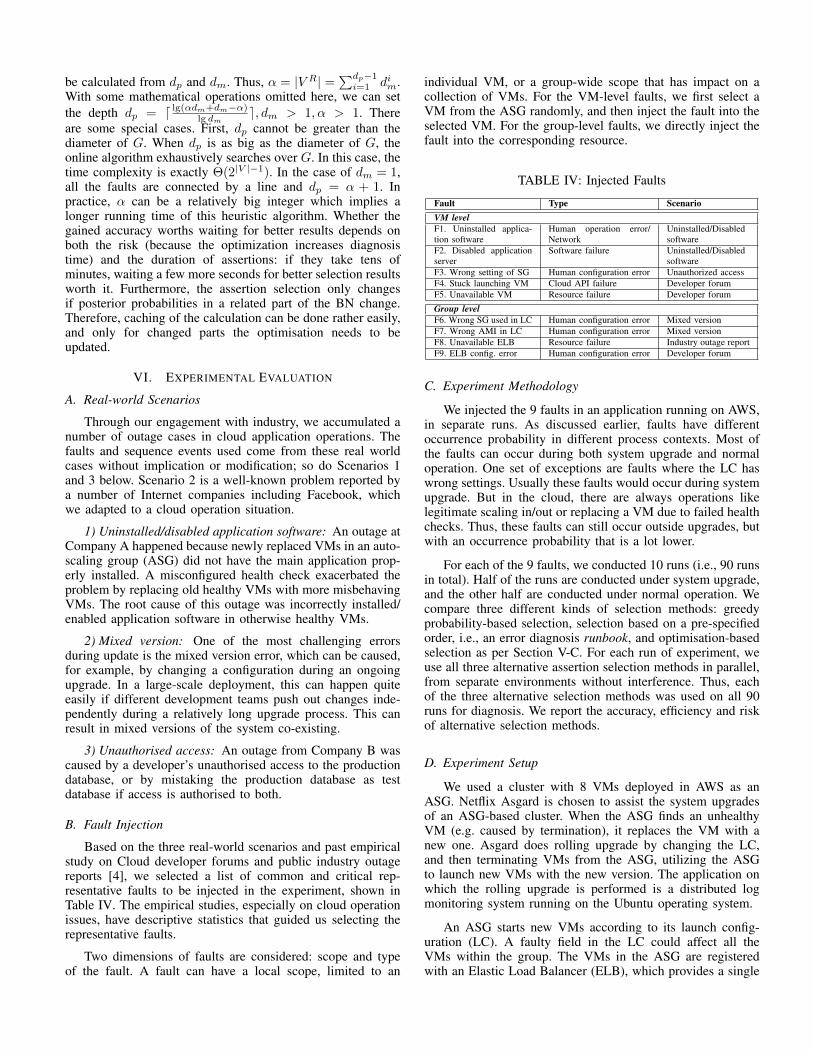
TABLE IV: Injected Faults

Fault Type ScenarioVM levelF1. Uninstalled applica-tion software

Human operation error/Network

Uninstalled/Disabledsoftware

F2. Disabled applicationserver

Software failure Uninstalled/Disabledsoftware

F3. Wrong setting of SG Human configuration error Unauthorized accessF4. Stuck launching VM Cloud API failure Developer forumF5. Unavailable VM Resource failure Developer forum

Group levelF6. Wrong SG used in LC Human configuration error Mixed versionF7. Wrong AMI in LC Human configuration error Mixed versionF8. Unavailable ELB Resource failure Industry outage reportF9. ELB config. error Human configuration error Developer forum

C. Experiment Methodology

We injected the 9 faults in an application running on AWS,in separate runs. As discussed earlier, faults have differentoccurrence probability in different process contexts. Most ofthe faults can occur during both system upgrade and normaloperation. One set of exceptions are faults where the LC haswrong settings. Usually these faults would occur during systemupgrade. But in the cloud, there are always operations likelegitimate scaling in/out or replacing a VM due to failed healthchecks. Thus, these faults can still occur outside upgrades, butwith an occurrence probability that is a lot lower.

For each of the 9 faults, we conducted 10 runs (i.e., 90 runsin total). Half of the runs are conducted under system upgrade,and the other half are conducted under normal operation. Wecompare three different kinds of selection methods: greedyprobability-based selection, selection based on a pre-specifiedorder, i.e., an error diagnosis runbook, and optimisation-basedselection as per Section V-C. For each run of experiment, weuse all three alternative assertion selection methods in parallel,from separate environments without interference. Thus, eachof the three alternative selection methods was used on all 90runs for diagnosis. We report the accuracy, efficiency and riskof alternative selection methods.

D. Experiment Setup

We used a cluster with 8 VMs deployed in AWS as anASG. Netflix Asgard is chosen to assist the system upgradesof an ASG-based cluster. When the ASG finds an unhealthyVM (e.g. caused by termination), it replaces the VM with anew one. Asgard does rolling upgrade by changing the LC,and then terminating VMs from the ASG, utilizing the ASGto launch new VMs with the new version. The application onwhich the rolling upgrade is performed is a distributed logmonitoring system running on the Ubuntu operating system.

An ASG starts new VMs according to its launch config-uration (LC). A faulty field in the LC could affect all theVMs within the group. The VMs in the ASG are registeredwith an Elastic Load Balancer (ELB), which provides a single

point of contact for incoming traffic. Thus, if the ELB becomesunavailable or is misconfigured, it will affect the whole ASG.

VMs within the ASG are associated with a security group(SG). SG is used to separate testing environment and produc-tion environment. A faulty rule within the SG could allow aresource in the testing environment to access the productionenvironment. The VMs are associated with a resource-basedIAM policy as well to define the permissions of users based onorganisational groups. The resource-based IAM policy workstogether with user-based one to restrict users’ AWS accessbased on their roles, such as developer or tester. Furthermore,access to VMs is based on an ssh key pair. Upgrading a VMcan include changing AMI, SG rules, key pair, IAM policy orother configurations, such as VM type or kernel ID.

E. Experiment Results

1) Accuracy: The diagnosis with all the three methods ofassertion selection achieved 100% accuracy if the injected faultwas not transient, meaning the root cause remained observableuntil a diagnosis finished. However, transient faults causedfalse negative cases in our diagnosis and thus, decreased theaccuracy. Transient faults are common in cloud applicationsdue to the sophisticated fault tolerance mechanisms at variouslevels. Whether a transient fault is detected depends on twofactors: diagnosis time and the assertion used to find thefault. For example, ASGs can be used for fault tolerance. Ifa VM becomes unavailable, the ASG will start a new VM toreplace the unavailable VM. Depending on what informationis required for diagnosis, the original fault may get lost due tothe replacement. Undiagnosed faults may come back.

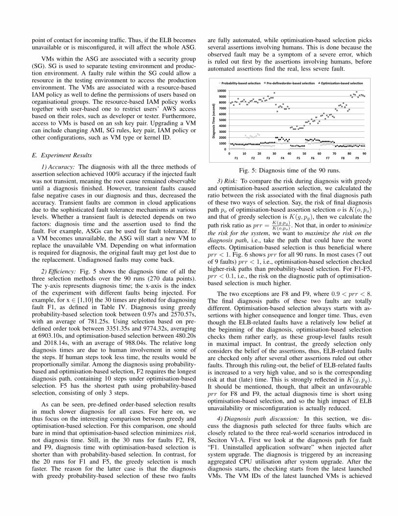
2) Efficiency: Fig. 5 shows the diagnosis time of all thethree selection methods over the 90 runs (270 data points).The y-axis represents diagnosis time; the x-axis is the indexof the experiment with different faults being injected. Forexample, for x ∈ [1,10] the 30 times are plotted for diagnosingfault F1, as defined in Table IV. Diagnosis using greedyprobability-based selection took between 0.97s and 2570.57s,with an average of 781.25s. Using selection based on pre-defined order took between 3351.35s and 9774.32s, averagingat 6903.10s, and optimisation-based selection between 480.20sand 2018.14s, with an average of 988.04s. The relative longdiagnosis times are due to human involvement in some ofthe steps. If human steps took less time, the results would beproportionally similar. Among the diagnosis using probability-based and optimisation-based selection, F2 requires the longestdiagnosis path, containing 10 steps under optimisation-basedselection. F5 has the shortest path using probability-basedselection, consisting of only 3 steps.

As can be seen, pre-defined order-based selection resultsin much slower diagnosis for all cases. For here on, wethus focus on the interesting comparison between greedy andoptimisation-based selection. For this comparison, one shouldbare in mind that optimisation-based selection minimizes risk,not diagnosis time. Still, in the 30 runs for faults F2, F8,and F9, diagnosis time with optimisation-based selection isshorter than with probability-based selection. In contrast, forthe 20 runs for F1 and F5, the greedy selection is muchfaster. The reason for the latter case is that the diagnosiswith greedy probability-based selection of these two faults

are fully automated, while optimisation-based selection picksseveral assertions involving humans. This is done because theobserved fault may be a symptom of a severe error, whichis ruled out first by the assertions involving humans, beforeautomated assertions find the real, less severe fault.

0  

1000  

2000  

3000  

4000  

5000  

6000  

7000  

8000  

9000  

10000  

0   10   20   30   40   50   60   70   80   90  

Diagno

sis  T

ime  (secon

d)  

Probability-­‐based  selecAon   Pre-­‐definedorder-­‐based  selecAon   OpAmizaAon-­‐based  selecAon  

F1                               F2                              F3                            F4                                F5                            F6                              F7                              F8                            F9    

Fig. 5: Diagnosis time of the 90 runs.

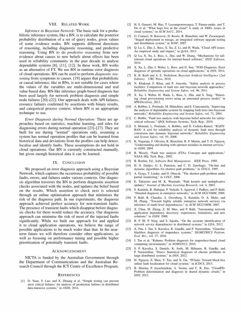
3) Risk: To compare the risk during diagnosis with greedyand optimisation-based assertion selection, we calculated theratio between the risk associated with the final diagnosis pathof these two ways of selection. Say, the risk of final diagnosispath po of optimisation-based assertion selection o is K(o, po)and that of greedy selection is K(g, pg), then we calculate thepath risk ratio as prr =

K(g,pg)K(o,po)

. Not that, in order to minimizethe risk for the system, we want to maximize the risk on thediagnosis path, i.e., take the path that could have the worsteffects. Optimisation-based selection is thus beneficial whereprr < 1. Fig. 6 shows prr for all 90 runs. In most cases (7 outof 9 faults) prr < 1, i.e., optimisation-based selection checkedhigher-risk paths than probability-based selection. For F1-F5,prr < 0.1, i.e., the risk on the diagnostic path of optimisation-based selection is much higher.

The two exceptions are F8 and F9, where 0.9 < prr < 8.The final diagnosis paths of these two faults are totallydifferent. Optimisation-based selection always starts with as-sertions with higher consequence and longer time. Thus, eventhough the ELB-related faults have a relatively low belief atthe beginning of the diagnosis, optimisation-based selectionchecks them rather early, as these group-level faults resultin maximal impact. In contrast, the greedy selection onlyconsiders the belief of the assertions, thus, ELB-related faultsare checked only after several other assertions ruled out otherfaults. Through this ruling-out, the belief of ELB-related faultsis increased to a very high value, and so is the correspondingrisk at that (late) time. This is strongly reflected in K(g, pg).It should be mentioned, though, that albeit an unfavourableprr for F8 and F9, the actual diagnosis time is short usingoptimisation-based selection, and so the high impact of ELBunavailability or misconfiguration is actually reduced.

4) Diagnosis path discussion: In this section, we dis-cuss the diagnosis path selected for three faults which areclosely related to the three real-world scenarios introduced inSeciton VI-A. First we look at the diagnosis path for fault“F1. Uninstalled application software” when injected aftersystem upgrade. The diagnosis is triggered by an increasingaggregated CPU utilisation after system upgrade. After thediagnosis starts, the checking starts from the latest launchedVMs. The VM IDs of the latest launched VMs is achieved

0  

1  

2  

3  

4  

5  

6  

7  

8  

0   10   20   30   40   50   60   70   80   90  

Ra.o

 between  Risk  of  P

roba

bility-­‐ba

sed  an

d  Op.

miza.

on-­‐base    

F1                            F2                                F3                              F4                              F5                          F6                                F7                            F8                              F9    

Fig. 6: Ratio between probability-based selection andoptimisation-based selection.

by the first automated assertion costing around 3s. Then thestatuses of the VMs are checked to identify the abnormalVM, which is an automated assertion, costing around 2s.After excluding the VM-level failure, the scope of the error isnarrowed down to application-level fault that causes the failureof ELB VM health checking. After automatically checking theapplication-level health, around 0.3s, we confirmed that thefault is at VM-level. There are many faults that could causeELB VM health checking to fail, such as ELB configurationerror, authentication problem, an application software is notinstalled or enabled among others. Here fault F1 has thehighest risk due to its higher probability caused by humanoperation error, network connection error or code repositorydown etc. Thus, the corresponding automated assertion is thefirst one to be checked at this level. Overall, the diagnosis pathof this fault includes 4n assertion checking, n is the numberof latest launched VMs. The average diagnosis time is 4.15sfor one VM. The risk of optimisation-based diagnosis is 364times of the risk of probability-based diagnosis on average.

The second one is the diagnosis path of fault “F7. WrongAMI in launch configuration” injected during system upgrade.After checking several assertions, we found out that an VMfails the application-level health check. The fault at the nextlevel with the highest risk is that “a VM is using an unexpectedAMI”. The VM is in an ASG (please refer to Fig. 3 for therelevant sub graph), Thus, one possibility is that the AMIconfiguration of launch configuration is not correct. It is alsopossible that the faulty VM is launched outside ASG with awrong AMI, and attached to ASG. During system upgrade,the far left branch is traversed first because LC is much morepossible to have problem and has larger consequence duringsystem upgrade. The average diagnosis time is 791s. If theerror is caused by a faulty VM being launched outside ASGand attached back to ASG, the confirmation of the fault mighthave up to 15 minutes delay for us to check the Cloudtrail3record to find when the VM is attached to the ASG by whom.The risk of optimisation-based diagnosis is 2 times of the riskof probability-based diagnosis on average.

The third one is the unauthorised access problem causedby fault “F3. Wrong setting of SG”. Similar to the diagnosis ofthe second fault, we first found out that a certain VM fails theapplication-level health check. The access problem is the faultat the next level with the second highest risk. To confirm the

3http://aws.amazon.com/cloudtrail/

access problem, the access log of the database deployed on theVM is checked manually, which may cost around 4 minutes.There are two faults that could cause the access problem,including wrong setting of SG and wrong IAM-policy setting.The first possibility is checked first and confirmed the rootcause. To check the SG setting, we first automatically comparethe current setting with a desired setting, and then manuallygo through the setting see if the setting is really correct. Theaverage diagnosis time of this fault is around 9 minutes. Onaverage, The risk of optimisation-based diagnosis is 36 timesof the risk of probability-based diagnosis.

VII. DISCUSSION AND LIMITATION

Variation in Diagnosis Time: The diagnosis time of a faultis dominated heavily by the execution time of the assertionson the diagnosis path. The assertions’ running times havea large variation. Automated assertions, e.g., those that canbe checked by calling cloud API(s), finish within seconds.However, there are assertions that need to check informationonly becomes available after some delay – e.g., CloudTraillogs, which shows up to 15 minutes delay. There are otherassertions that are hard to automate, e.g., checking severallogs or checking complicated configurations. And time spenton assertions that involve human interaction is more varied,among others because it depends on the operator’s capability.

Multiple Faults: If multiple faults must occur together tocause a failure, our diagnosis continues until all the requiredfaults are identified. However, if not all the root faults arerequired to cause the failure, the current diagnosis methodstops after identifying one of the faults causing the failure.We plan to extend the diagnosis algorithm for these cases.

Overlapping Faults: Some root faults are overlapping sincewe consider faults with differing scopes. Several group-levelfaults cause several VMs to turn into erroneous states. Thus,if we checked for VM-level faults, we could miss a group-level cause if we stopped after one VM-level fault is identified.Optimisation-based diagnosis avoids this situation because italways check for faults with higher consequence first.

Limitations: There are some obvious limitations of ourapproach. First, the fault tree still needs to be constructed andconverted to BN manually and new faults need to be added. Tomake this approach applicable for systems with many differenttypes of faults, automation in these aspects is needed. For cloudoperations, we observed the number of faults to be limited.

The approach primarily applies to non-transient faults.Transient faults can only be diagnosed if the duration dur-ing which they are observable is longer than the time untildiagnosis checks for them. Also, the approach relies on thecompleteness of the models – faults that are not modelled,or where the assertions are unable to find the fault, will notbe found. The perfect diagnosis accuracy we observed in ourexperiments can only be achieved with complete models.

Acquiring probabilities is always difficult, especially whenspecific to a single organisation or operation. We believe thereare commonalities among the different types of operations,reflected in their frequency of using the cloud APIs forinfrastructure and configurations. Also, as argued above, exactprobabilities are not a requirement for successful diagnosis.

VIII. RELATED WORK

Inference in Bayesian Network: The basic task for a proba-bilistic inference system, like a BN, is to calculate the posteriorprobability distribution of a set of query nodes, given valuesof some evidence nodes. BN supports different directionsof reasoning, including diagnostic reasoning, and predictivereasoning. Using BN to do predictive reasoning from newevidence about causes to new beliefs about effects has beenused in reliability community in the past decade to analysedependable systems [8], [11], [12]. In these work, BN worksas an alternative of FT. We use BN in runtime error diagnosisof cloud operations. BN can be used to perform diagnostic rea-soning from symptoms to causes. [19] argues that probabilisticor causal inference, like in BNs, is not suitable for cases wherethe values of the variables are multi-dimensional and realvalue-based data. BN-like inference graph-based diagnosis hasbeen used largely for network problem diagnosis and simplenode failures [20]–[22]. Our approach deals with API failures,resource failures confirmed by assertions with binary results,and categorical process context, where BN is an appropriatetechnique to use.

Error Diagnosis during Normal Operation: There are ap-proaches based on statistics, machine learning, and rules fordiagnosing errors during normal operation [23]–[27]. They arebuilt for use during “normal” operations only, assuming asystem has normal operation profiles that can be learned fromhistorical data and deviations from the profiles can help detect,localise and identify faults. These assumptions do not hold incloud operations. Our BN is currently constructed manually,but given enough historical data it can be learned.

IX. CONCLUSION

We proposed an error diagnosis approach using a BayesianNetwork, which captures the occurrence probability of possiblefaults, errors, and failures under various contexts. Our diagno-sis algorithm traverses the BN to perform diagnostic assertionchecks associated with the nodes, and updates the belief basedon the results. Which assertion to check next is selectedthrough an online optimisation approach that minimises therisk of the diagnosis path. In our experiments, the diagnosisapproach achieved perfect accuracy for non-transient faults.The presence of transient faults which disappear before diagno-sis checks for them would reduce the accuracy. Our diagnosisapproach can minimise the risk of most of the injected faultssignificantly. While we built our approach for and appliedit to cloud application operations, we believe the range ofpossible applications to be much wider than that. In the near-term future we will therefore consider other applications, aswell as focusing on performance tuning and possible higherprioritization of potentially transient faults.

ACKNOWLEDGMENT

NICTA is funded by the Australian Government throughthe Department of Communications and the Australian Re-search Council through the ICT Centre of Excellence Program.

REFERENCES

[1] D. Yuan, Y. Luo, and X. Zhuang et al, “Simple testing can preventmost critical failures: An analysis of production failures in distributeddata-intensive systems,” in OSDI, 2014.

[2] H. S. Gunawi, M. Hao, T. Leesatapornwongsa, T. Patana-anake, and T.Do et al, “What bugs live in the cloud? A study of 3000+ issues incloud systems,” in ACM SoCC, 2014.

[3] O. Crameri, N. Knezevic, D. Kostic, R. Bianchini, and W. Zwaenepoel,“Staged deployment in mirage, an integrated software upgrade testingand distribution system,” in SOSP, 2007.

[4] Q. Lu, L. Zhu, L. Bass, X. Xu, Z. Li, and H. Wada, “Cloud API issues:An empirical study and impact,” in QoSA, 2013.

[5] Q. Lu, X. Xu, L. Bass, L. Zhu, and W. Zhang, “Mechanisms for tail-tolerant cloud operations for internet-based software,” IEEE Software,2014.

[6] X. Xu, L. Zhu, I. Weber, L. Bass, and D. Sun, “POD-Diagnosis: Errordiagnosis of sporadic operations on cloud applications,” in DSN, 2014.

[7] K. B. Korb and A. E. Nicholson, Bayesian Artificial Intelligence (2ndEdition). CRC Press, 2010.

[8] N. Khakzad, F. Khan, and P. Amyotte, “Safety analysis in processfacilities: Comparison of fault tree and bayesian network approaches,”Reliability Engineering and System Safety, vol. 96, 2011.

[9] X. Xu, I. Weber, H. Wada, L. Bass, L. Zhu, and S. Teng, “Detect-ing cloud provisioning errors using an annotated process model,” inMW4NextGen, 2013.

[10] A. Bobbio, L. Portinale, M. Minichino, and E. Ciancamerla, “Improvingthe analysis of dependable systems by mapping fault trees into bayesiannetworks,” Reliability Engineering and System Safety, vol. 71, 2001.

[11] C. Hobbs, “Fault tree analysis with bayesian belief networks for safety-critical software,” QNX Software Systems, Tech. Rep., 2010.

[12] S. Montani, L. Portinale, A. Bobbio, and D. Codetta-Raiteri, “RADY-BAN: A tool for reliability analysis of dynamic fault trees throughconversion into dynamic bayesian networks,” Reliability Engineeringand System Safety, vol. 93, 2008.

[13] K. Nagaraja, F. Oliveira, R. Bianchini, R. P. Martin, and T. D. Nguyen,“Understanding and dealing with operator mistakes in internet services,”in OSDI, 2004.

[14] B. Wesely, “Fault tree analysis (FTA): Concepts and applications,”NASA HQ, Tech. Rep., 2002.

[15] B. Boehm, Ed., Software Risk Management. IEEE Press, 1989.[16] H. N. Djidjev, G. E. Pantziou, and C. D. Zaroliagis, “On-line and

dynamic algorithms for shortest path problems,” in STACS, 1995.[17] A. Gyrgy, T. Linder, and G. Ottucsk, “The shortest path problem under

partial monitoring,” in COLT, 2006.[18] E. Takimoto and M. K. Warmuth, “Path kernels and multiplicative

updates,” Journal of Machine Learning Research, vol. 4, 2003.[19] S. Kandula, R. Mahajan, P. Verkaik, S. Agarwal, J. Padhye, and P. Bahl,

“Detailed diagnosis in enterprise networks,” in ACM SIGCOMM, 2009.[20] P. Bahl, R. Chandra, A. Greenberg, S. Kandula, D. A. Maltz, and

M. Zhang, “Towards highly reliable enterprise network services viainference of multi-level dependencies,” in ACM SIGCOMM, 2007.

[21] X. Chen, M. Zhang, Z. M. Mao, and P. Bahl, “Automating networkapplication dependency discovery: experiences, limitations, and newsolutions,” in OSDI, 2008.

[22] B. P. III, P. Ning, and S. Jajodia, “On the accurate identification ofnetwork service dependencies in distributed systems,” in LISA, 2012.

[23] X. Pan, J. Tan, S. Kavulya, R. Gandhi, and P. Narasimhan, “Ganesha:blackbox diagnosis of mapreduce systems,” SIGMETRICS Perform.Eval. Rev., vol. 37, 2010.

[24] J. Tan et al, “Kahuna: Problem diagnosis for mapreduce-based cloudcomputing environments,” in NOMS2012, 2010.

[25] S. P. Kavulya, S. Daniels, K. Joshi, M. Hiltunen, R. Gandhi, andP. Narasimhan, “Draco: Statistical diagnosis of chronic problems inlarge distributed systems,” in DSN, 2012.

[26] H. Nguyen, Z. Shen, Y. Tan, and X. Gu, “FChain: Toward black-boxonline fault localization for cloud systems,” in ICDCS, 2013.

[27] B. Sharma, P. Jayachandran, A. Verma, and C. R. Das, “CloudPD:Problem determination and diagnosis in shared dynamic clouds,” inDSN, 2013.