error estimates for reduced order mhd model …20 = 100 and s = 10 initial velocity ﬁeld: u 1

Error Estimates for Reduced Order MHD Model basedon POD

S.S. Ravindran

University of Alabama in Huntsville, USAhttp:ultra.uah.edu/ravindra

[email protected]

INRIA Workshop: Industrial Applications of Low Order Models Basedon POD

Bordeaux, 2008

Ravindran (University of Alabama) Error Estimates for a Reduced Order MHD Model POD 2008 1 / 23

Outline of the Talk

Outline of talk:

Magnetohydrodynamic (MHD) Equations

Finite Element Galerkin Scheme and Error Estimates

POD Galerkin Scheme and Error Estimates

Computational Implementation: Control of MHD

Finite element model & optimal controlLow dimensional model & optimal control


MHD equations

Model for viscous incompressible electrically conducting flows

u-velocity; p-pressure; B-magnetic field

∂u

∂t− 1

Re∇2u + (u · ∇)u + ∇p − S(curl B) × B = f in Ω × (0,T ]

∂B∂t

+ 1Rem

curl (curl B) − curl (u × B) = curl j in Ω × (0,T ]

∇ · u = 0 and ∇ · B = 0 in Ω × (0,T ]

Boundary values:u = 0 , B · n = 0 and (curl B) × n = 0 on ∂Ω × (0,T ]

Initial values: u(x, 0) = 0 and B(x, 0) = 0 in Ω ,

Re- Reynolds number; Rem- Magnetic Reynolds number;S- coupling parameter


MHD equations

Functional Framework

Divergence free spaces

Hu = HB := w ∈ L2(Ω) : ∇ · w = 0 and w · n = 0 on ∂Ω ,

Vu := Hu ∩H10(Ω) and VB := HB ∩H1

n(Ω) .

H := Hu × HB and V := Vu × VB with inner-products

(χ1,χ2)H :=

∫

Ωu1 · u2 dx + S

∫

ΩB1 · B2 dx

(χ1,χ2)V :=1

Re

∫

Ω∇u1 : ∇u2 dx +

S

Rem

∫

Ωcurl B1 · curl B2 dx

Poincare type inequality:

η‖(u,B)‖2H ≤ ‖(u,B)‖2

V ∀(u,B) ∈ V , where η := min

ηu

Re,ηB

Rem

.


MHD equations

Weak Form of MHD Equations

Weak form:

(∂χ

∂t,w)H + a(χ,w) + b(χ,χ,w) = (F,w)H , ∀χ ∈ V

Here bilinear form

a(χ1,χ2) =1

Re

∫

Ω∇u1 : ∇u2 dx +

S

Rem

∫

Ωcurl B1 · curl B2 dx

and tri-linear form

b(χ1,χ2,χ3) =∫Ω(u1 · ∇)u2 · u3 dx− S

∫Ω curl B2 × B1 · u3 dx

−S∫Ω u2 × B1 · curl B3 dx

∀χi = (ui ,Bi ) ∈ V

Note ‖ · ‖v = (a(·, ·)) 12


MHD equations

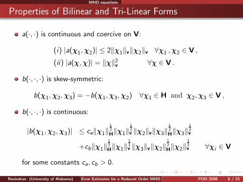
Properties of Bilinear and Tri-Linear Forms

a(·, ·) is continuous and coercive on V:

(i) |a(χ1,χ2)| ≤ 2‖χ1‖v‖χ2‖v ∀χ1 ,χ2 ∈ V ,

(ii) |a(χ,χ)| = ‖χ‖2v ∀χ ∈ V .

b(·, ·, ·) is skew-symmetric:

b(χ1,χ2,χ3) = −b(χ1,χ3,χ2) ∀χ1 ∈ H and χ2,χ3 ∈ V ,

b(·, ·, ·) is continuous:

|b(χ1,χ2,χ3)| ≤ ca‖χ1‖12H‖χ1‖

12v ‖χ2‖v‖χ3‖

12H‖χ3‖

12v

+cb‖χ1‖12H‖χ1‖

12v ‖χ3‖v‖χ2‖

12H‖χ2‖

12v ∀χi ∈ V

for some constants ca, cb > 0.


Finite Element Error Estimate

Finite Element Glerkin Scheme and Error Estimate

Divergence-free finite element space Vh ⊂ V . Let χhn ≈ χh(tn).

Fully implicit backward Euler in time scheme: seek χhn ∈ Vh such that

(χn

h − χn−1h

k,wh)H+a(χn

h,wh)+b(χnh,χ

nh,wh) = (Fn,wh)H ,∀wh ∈ Vh

Appriori estimate:

‖χnh‖2

H + k

n∑

i=1

‖χih‖2

V ≤ kη2n∑

i=1

‖Fi‖2H

Finite element error estimate:

‖χ − χnh‖H ≤ C (σ−1(tn)k + hp)


POD Galerkin Error Estimate

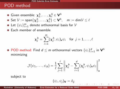
POD method

Given ensemble: χh1, . . . ,χ

hℓ ∈ Vh

Set V := spanχh1, . . . ,χ

hℓ ⊂ Vh, m := dimV ≤ ℓ

Let ψimi=1 denote orthonormal basis for V

Each member of ensemble

χhj =

m∑

i=1

(χhj , ψi )vψi for j = 1, . . . , ℓ

POD method: Find d ≤ m orthonormal vectors ψidi=1 in Vh

minimizing

J (ψ1, . . . , ψd) =1

ℓ

ℓ∑

j=1

∥∥∥∥∥χhj −

d∑

i=1

(χhj , ψi )vψi

∥∥∥∥∥

2

v

subject to(ψi , ψj )V = δij



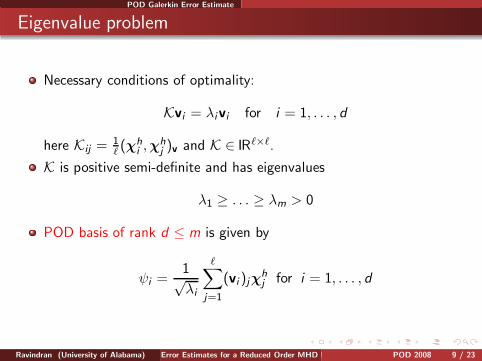
Eigenvalue problem

Necessary conditions of optimality:

Kvi = λivi for i = 1, . . . , d

here Kij = 1ℓ(χh

i ,χhj )v and K ∈ RI ℓ×ℓ.

K is positive semi-definite and has eigenvalues

λ1 ≥ . . . ≥ λm > 0

POD basis of rank d ≤ m is given by

ψi =1√λi

ℓ∑

j=1

(vi )jχhj for i = 1, . . . , d



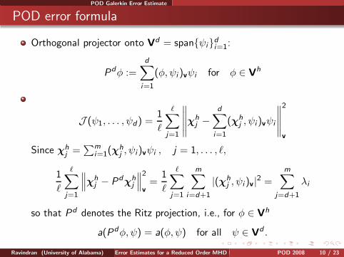
POD error formula

Orthogonal projector onto Vd = spanψidi=1:

Pdφ :=

d∑

i=1

(φ,ψi )vψi for φ ∈ Vh

J (ψ1, . . . , ψd) =1

ℓ

ℓ∑

j=1

∥∥∥∥∥χhj −

d∑

i=1

(χhj , ψi )vψi

∥∥∥∥∥

2

v

Since χhj =

∑mi=1(χ

hj , ψi )vψi , j = 1, . . . , ℓ,

1

ℓ

ℓ∑

j=1

∥∥∥χhj − Pdχh

j

∥∥∥2

v=

1

ℓ

ℓ∑

j=1

m∑

i=d+1

|(χhj , ψi )v|2 =

m∑

j=d+1

λi

so that Pd denotes the Ritz projection, i.e., for φ ∈ Vh

a(Pdφ,ψ) = a(φ,ψ) for all ψ ∈ Vd .



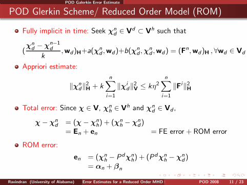
POD Glerkin Scheme/ Reduced Order Model (ROM)

Fully implicit in time: Seek χnd ∈ Vd ⊂ Vh such that

(χn

d − χn−1d

k,wd)H+a(χn

d ,wd)+b(χnd ,χ

nd ,wd) = (Fn,wd)H ,∀wd ∈ Vd

Appriori estimate:

‖χnd‖2

H + k

n∑

i=1

‖χid‖2

V ≤ kη2n∑

i=1

‖Fi‖2H

Total error: Since χ ∈ V, χnh ∈ Vh and χn

d ∈ Vd ,

χ − χnd = (χ − χn

h) + (χnh − χn

d)= En + en = FE error + ROM error

ROM error:

en = (χnh − Pdχn

h) + (Pdχnh − χn

d)= αn + βn



Reduced Order Model Error

ROM error equation:

(en − en−1, vd )H + ka(en, vd ) + k[b(χnh,χ

nh, vd)− b(χn

d ,χnd , vd)] = 0 .

Take vd = βn and note that

(I) Since a(αn,βn) = 0 by Ritz projection condition,

a(en,βn) = a(en, en) − a(αn,αn) = ‖en‖2v − ‖αn‖2

v

(II)

|b(χnh,χ

nh,βn) −b(χn

d ,χnd ,βn)|

= |b(und , en,αn) + b(en,u

hn,αn) − b(en,u

nh, en)|

≤ 12‖en‖2

v + C0‖αn‖2v + C1‖en‖2

H

by Holder inequality followed by Sobolve and Young’s inequalities.



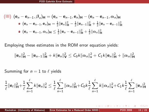
(III) (en − en−1,βn)H = (en − en−1, en)H − (en − en−1,αn)H

(en − en−1, en)H = 12‖en‖2

H − 12‖en−1‖2

H + 12‖en − en−1‖2

H

(en − en−1,αn)H ≤ 12‖en − en−1‖2

H + 12‖αn‖2

H

Employing these estimates in the ROM error equation yields:

‖en‖2H − ‖en−1‖2

H + k‖en‖2V ≤ C0k‖αn‖2

v + C1k‖en‖2H + ‖αn‖2

H

Summing for n = 1 to ℓ yields

1

ℓ‖eℓ‖2

H+1

ℓ

ℓ∑

n=1

k‖en‖2v ≤ 1

ℓ

ℓ∑

n=1

‖αn‖2H+C0k

1

ℓ

ℓ∑

n=1

k‖αn‖2v+C1k

1

ℓ

ℓ∑

n=1

‖en|2H



Assuming k satisfies C1k ≤ θ < 1 and applying Discrete GronwallInequality yields

1 − θ

ℓ‖eℓ‖2

H +k

l

ℓ∑

n=1

‖en‖2v ≤ eθ(

1

η+ C0k)

m∑

n=d+1

λn

Error estimate:

‖χ − χnd‖H ≤ ‖χ − χn

h‖H + ‖χnh − χn

d‖H

≤ C (σ−1(tn)k + hp) +[

ℓ1−θ

eθ( 1η

+ C0k)∑m

n=d+1 λn

] 12



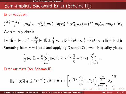
Semi-implicit Backward Euler (Scheme II):

Error equation:

(χn

d − χn−1d

k,wd)H+a(χn

d ,wd)+b(χn−1d ,χn

d ,wd) = (Fn,wd)H ,∀wd ∈ Vd

We similarly obtain

‖en‖2H − ‖en−1‖2

H +5k

4‖en‖2

V ≤ k

4‖en−1‖2

V + C0k‖αn‖2v + C2k‖en−1‖2

H + ‖αn‖2H

Summing from n = 1 to ℓ and applying Discrete Gronwall inequality yields

1

ℓ‖eℓ‖2

H +k

l

ℓ∑

n=1

‖en‖2v ≤ eC2k(

1

η+ C0k)

m∑

n=d+1

λn

Error estimate (for Scheme II):

‖χ − χnd‖H ≤ C (σ−1(tn)k + hp) +

[

ℓeC2k

(1

η+ C0k

) m∑

n=d+1

λn

] 12


Computational Application Optimal Control of MHD: Velocity tracking

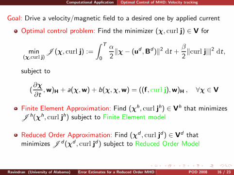
Goal: Drive a velocity/magnetic field to a desired one by applied current

Optimal control problem: Find the minimizer (χ, curl j) ∈ V for

min(χ,curl j)

J (χ, curl j) :=

∫ T

0

α

2‖χ − (ud ,Bd)‖2

dt +β

2‖curl j|‖2

dt,

subject to

(∂χ

∂t,w)H + a(χ,w) + b(χ,χ,w) = ((f, curl j),w)H , ∀χ ∈ V

Finite Element Approximation: Find (χh, curl jh) ∈ Vh that minimizesJ h(χh, curl jh) subject to Finite Element model

Reduced Order Approximation: Find (χd , curl jd) ∈ Vd thatminimizes J d(χd , curl jd) subject to Reduced Order Model


Computational Application Optimality System

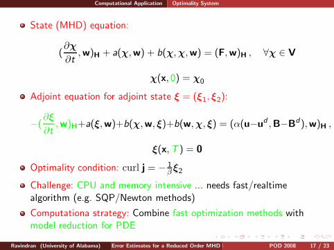
State (MHD) equation:

(∂χ

∂t,w)H + a(χ,w) + b(χ,χ,w) = (F,w)H , ∀χ ∈ V

χ(x, 0) = χ0

Adjoint equation for adjoint state ξ = (ξ1, ξ2):

−(∂ξ

∂t,w)H+a(ξ,w)+b(χ,w, ξ)+b(w,χ, ξ) = (α(u−ud ,B−Bd),w)H ,

ξ(x,T ) = 0

Optimality condition: curl j = − 1βξ2

Challenge: CPU and memory intensive ... needs fast/realtimealgorithm (e.g. SQP/Newton methods)

Computationa strategy: Combine fast optimization methods withmodel reduction for PDE


Computational Application Finite Element Computation

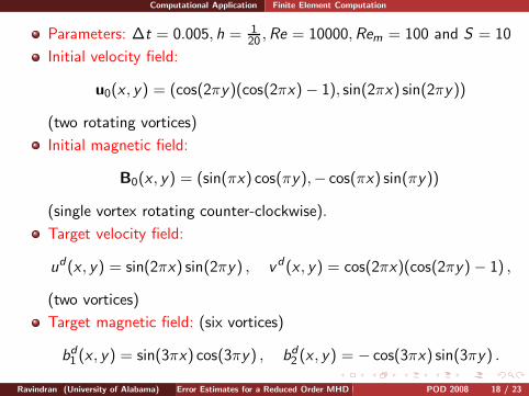
Parameters: ∆t = 0.005, h = 120 ,Re = 10000,Rem = 100 and S = 10

Initial velocity field:

u0(x , y) = (cos(2πy)(cos(2πx) − 1), sin(2πx) sin(2πy))

(two rotating vortices)

Initial magnetic field:

B0(x , y) = (sin(πx) cos(πy),− cos(πx) sin(πy))

(single vortex rotating counter-clockwise).

Target velocity field:

ud(x , y) = sin(2πx) sin(2πy) , vd(x , y) = cos(2πx)(cos(2πy) − 1) ,

(two vortices)

Target magnetic field: (six vortices)

bd1 (x , y) = sin(3πx) cos(3πy) , bd

2 (x , y) = − cos(3πx) sin(3πy) .


Computational Application Optimal controlled magnetic field (Finite Element computation)

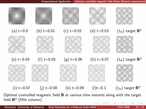
(a) t=0.0 (b) t=0.01 (c) t=0.02 (d) t=0.03 (tm) target Bd

(e) t=0.04 (f) t=0.05 (g) t=0.06 (h) t=0.07 (tm) target Bd

(i) t=0.07 (j) t=0.08 (k) t=0.09 (l)t=0.1 (tm) target Bd

Optimal controlled magnetic field B at various time instants along with the targetfield Bd (fifth column)


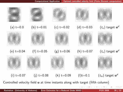
Computational Application Optimal controlled velocity field (Finite Element computation)

(a) t=0.0 (b) t=0.01 (c) t=0.02 (d) t=0.03 (tu) target ud

(e) t=0.04 (f) t=0.05 (g) t=0.06 (h) t=0.07 (tu) target ud

(i) t=0.07 (j) t=0.08 (k) t=0.09 (l)t=0.1 (tm) target ud

Controlled velocity field u at time instants along with target (fifth column)


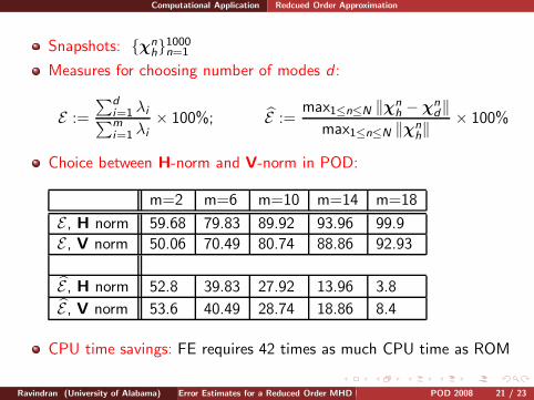
Computational Application Redcued Order Approximation

Snapshots: χnh1000

n=1

Measures for choosing number of modes d :

E :=

∑di=1 λi∑mi=1 λi

× 100%; E :=max1≤n≤N ‖χn

h − χnd‖

max1≤n≤N ‖χnh‖

× 100%

Choice between H-norm and V-norm in POD:

m=2 m=6 m=10 m=14 m=18

E , H norm 59.68 79.83 89.92 93.96 99.9

E , V norm 50.06 70.49 80.74 88.86 92.93

E , H norm 52.8 39.83 27.92 13.96 3.8

E , V norm 53.6 40.49 28.74 18.86 8.4

CPU time savings: FE requires 42 times as much CPU time as ROM


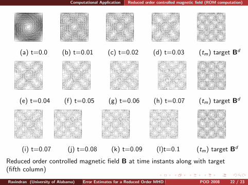
Computational Application Reduced order controlled magnetic field (ROM computation)

(a) t=0.0 (b) t=0.01 (c) t=0.02 (d) t=0.03 (tm) target Bd

(e) t=0.04 (f) t=0.05 (g) t=0.06 (h) t=0.07 (tm) target Bd

(i) t=0.07 (j) t=0.08 (k) t=0.09 (l)t=0.1 (tm) target Bd

Reduced order controlled magnetic field B at time instants along with target(fifth column)


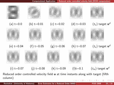
Computational Application Reduced order controlled velocity field (ROM computation)

(a) t=0.0 (b) t=0.01 (c) t=0.02 (d) t=0.03 (tu) target ud

(e) t=0.04 (f) t=0.05 (g) t=0.06 (h) t=0.07 (tu) target ud

(i) t=0.07 (j) t=0.08 (k) t=0.09 (l)t=0.1 (tm) target ud

Reduced order controlled velocity field u at time instants along with target (fifthcolumn)


error estimates for reduced order mhd model …20 = 100 and s = 10 initial velocity ﬁeld: u 1

Documents